


Highlights
What are the main findings?
- A graph-based mixture-of-experts (GMoE) multi-task learning framework with spatial-block validation achieved the highest predictive performance for As, Cd, Cu, and Hg contamination classes in European topsoils, while providing a more rigorous assessment of spatial generalization than conventional random sampling.
- Soil properties and hydroclimatic factors were identified as the dominant controls of heavy metal spatial heterogeneity, whereas the relative importance of environmental and anthropogenic drivers varied among metals.
What are the implications of the main findings?
- The proposed GMoE framework enables simultaneous prediction of multiple heavy metals within a single model, avoiding the repeated development and parameter optimization of separate models for individual elements.
- Spatial-block validation reduces performance overestimation caused by spatial autocorrelation and provides a more reliable evaluation framework for large-scale soil contamination mapping in geographically independent regions.
Abstract
Continental-scale assessment of soil heavy metal contamination is complicated by the contrasting environmental behaviour of individual metals and by spatial autocorrelation, which can lead to overly optimistic model evaluation. This study assessed As, Cu, Hg and Cd contamination in European topsoils using a harmonized 500 m dataset integrating soil properties, hydroclimatic and topographic conditions, socioeconomic indicators and anthropogenic emission sources. A graph-based mixture-of-experts (GMoE) model was used to jointly learn shared and metal-specific contamination patterns, while spatial-block hold-out testing evaluated its transferability to geographically independent regions. The model achieved the highest accuracy and macro-F1 among the evaluated approaches for all four metals, with the clearest improvements for As and Cu. Accuracy reached 76.96% for As and 75.43% for Cu, exceeding multi-gate mixture-of-experts (MMoE) by 4.79 and 2.86 percentage points, respectively. Routing diagnostics indicated broad but differentiated expert participation rather than reliance on a single expert. Spatial attribution further revealed that soil properties and hydroclimatic conditions strongly influenced contamination heterogeneity, whereas anthropogenic-source signals were more evident for As and Cd. These findings show that European topsoil contamination reflects both environmental filtering and source-related inputs, and demonstrate the value of combining spatially transferable multi-metal prediction with driver attribution for large-scale soil contamination assessment.
1. Introduction
Soil heavy metal contamination has become a growing environmental concern worldwide, posing serious threats to ecosystem stability, agricultural sustainability, and human health [1,2,3]. In Europe, rapid industrialization, intensive agricultural practices, and urban expansion have led to widespread accumulation of toxic metals such as arsenic (As), cadmium (Cd), copper (Cu) and mercury (Hg), which are among the most environmentally relevant and frequently monitored metals in European soils [4]. These pollutants are persistent, non-biodegradable, and easily transferred through soil–water–plant systems, causing long-term ecological risks and food-chain enrichment [5,6]. Accurately predicting their spatial distribution and concentration levels is thus crucial for effective risk assessment, remediation planning, and sustainable land management.
Previous studies have commonly used pollution indices, geostatistical interpolation, conventional statistical models and machine-learning approaches to assess soil heavy metal contamination and map regional pollution patterns [1,7,8,9,10]. Machine learning has improved the capacity to model nonlinear relationships between metal concentrations and heterogeneous environmental predictors, including soil properties, climate, topography and anthropogenic inputs [11,12,13,14]. However, many existing applications remain pollutant-specific, with models calibrated separately for individual metals [15,16]. This leads to repeated training of separate metal-specific models on the same regional dataset.
Building on this limitation, multi-output and multi-task learning provide a route for modelling several soil metals within a unified framework rather than through independent single-metal models [17,18]. However, their effectiveness depends on task relatedness, because heavy metals differ in geochemical behaviour, mobility, source pathways and spatial response patterns. Excessive or poorly controlled sharing may therefore cause task interference or negative transfer when shared environmental gradients coexist with pollutant-specific regional processes [18]. Mixture-of-experts (MoE) architectures offer a more flexible solution by allowing expert subnetworks to specialize in different input regimes while gating mechanisms adaptively combine their outputs [19,20]. In soil pollution research, a multi-gate mixture-of-experts (MMoE) network has been used to jointly identify heavy metal, volatile organic compound (VOC), and semi-volatile organic compound (SVOC) pollution at potentially contaminated sites, supporting the relevance of expert-based multi-task learning for complex soil contamination problems [21,22]. In a conventional MoE model, a single gating network combines the outputs of multiple experts for prediction. By contrast, MMoE extends this design to multi-task settings by using task-specific gates over a shared pool of experts, allowing different tasks to weight the same experts differently [22]. However, these expert-based architectures may still suffer from imbalanced expert utilization, such that some experts receive limited training signal whereas others are repeatedly selected [22]. Building on this framework, graph-based mixture-of-experts (GMoE) introduces graph-based routing and expert regularization to improve expert collaboration and load balance [23].
However, most existing machine-learning studies rely on random data splitting, which may overestimate predictive performance by allowing spatially autocorrelated samples to appear in both training and testing sets [21,22,24]. Large-scale soil heavy metal data are spatially autocorrelated, and neighbouring samples often share similar soil, climatic, topographic and anthropogenic conditions. Random train-test splitting may therefore evaluate local interpolation within spatially clustered neighbourhoods rather than transferability to unseen regions, leading to overly optimistic performance estimates [25,26,27]. Spatial block validation provides a more conservative assessment of whether the model can generalize beyond the spatial patterns observed during training [28]. At the same time, prediction-oriented machine learning models often provide limited insight into the environmental and anthropogenic factors underlying soil contamination patterns [29,30,31]. Geodetector provides a complementary attribution approach by quantifying the explanatory power of individual factors and their interactions on spatially stratified heterogeneity, without requiring assumptions of linearity or normality [32,33,34]. Combining spatially validated GMoE prediction with Geodetector attribution therefore links two related but distinct objectives: transferable multi-metal prediction and identification of dominant pollution drivers.
To address these gaps, this study develops a spatially validated GMoE–Geodetector framework for the prediction and attribution of As, Cu, Hg and Cd contamination in European topsoils. A harmonized 500 m gridded dataset was constructed by integrating soil physicochemical properties, hydroclimatic and topographic conditions, socioeconomic indicators and anthropogenic emission sources. The study addresses three objectives: (1) to evaluate the spatial transferability of GMoE-based multi-metal classification using spatial-block hold-out testing; (2) to characterize expert specialization, routing allocation and load-balancing behaviour; and (3) to quantify the explanatory power of environmental and anthropogenic factors for the spatial stratified heterogeneity of individual metals. This framework integrates spatially transferable prediction with spatial attribution to support continental-scale soil contamination assessment.
2. Materials and Methods
2.1. Study Area
This study focused on the European continent, which encompasses diverse environmental conditions across Mediterranean, Continental, Atlantic, and Boreal biogeographical regions. The European landscape is characterized by varying degrees of anthropogenic influence and geological backgrounds, including both densely populated industrial zones and rural agricultural landscapes with different management regimes. The target variables were the concentrations of 4 heavy metal elements (As, Cu, Hg and Cd) in European soils [7,35,36,37], obtained from the Land Use/Cover Area Frame Survey (LUCAS) topsoil database.
2.2. Datasets
This study utilized a comprehensive dataset comprising 40 predictor variables to characterize the environmental, physical, chemical, and anthropogenic factors potentially influencing heavy metal distribution in European soils. These variables were systematically categorized into six distinct groups.
(1) Soil physical properties obtained from the LUCAS database [38], including clay content (%), silt content (%), sand content (%), fraction of coarse fragments (Cfrag, %), bulk density (BD, Mg/m3), USDA texture class (TextureUSDA), and available water capacity (AWC).
(2) Soil chemical properties derived from the LUCAS database [39], including pH (measured in H2O), pH CaCl (soil pH measured in 0.01 M CaCl2 solution), cation exchange capacity (CEC), calcium carbonates (CaCO3), C:N ratio (C:N), nitrogen (N), phosphorus (P), and potassium (K).
(3) Climate variables extracted from the TerraClimate dataset for 2009 [40], encompassing downward surface shortwave radiation (SRAD), maximum and minimum temperature (Tmax, Tmin), vapour pressure (VP), wind speed (WS), vapour pressure deficit (VPD), Palmer Drought Severity Index (PDSI), actual evapotranspiration (AET), climate water deficit (DEF), potential evapotranspiration (PET), precipitation (PPT), runoff, and soil moisture (SM).
(4) Anthropogenic emission sources, which represent direct or indirect human-related inputs of heavy metals into the environment. Industrial emission variables were derived from enterprise-level release records in the European Pollutant Release and Transfer Register (E-PRTR) [41], and were further classified according to the reported release medium (ReleaseMediumName), because emission magnitudes and environmental pathways differ substantially among air, soil, and water releases. Accordingly, medium-specific industrial emission indicators were constructed, including industrial As emissions to air (Ind. As (Air)), industrial As emissions to soil (Ind. As (Soil)), industrial Cd emissions to air (Ind. Cd (Air)), industrial Cd emissions to soil (Ind. Cd (Soil)), industrial Cd emissions to water (Ind. Cd (Water)), industrial Cu emissions to air (Ind. Cu (Air)), industrial Cu emissions to soil (Ind. Cu (Soil)), industrial Cu emissions to water (Ind. Cu (Water)), and industrial Hg emissions to soil (Ind. Hg (Soil)). Mining activities from the European Geological Data Infrastructure [42] were used to characterize potential mining-related sources, while road network density derived from OpenStreetMap via Geofabrik [43] was used as a proxy for traffic-related emissions.
(5) Socioeconomic drivers, which reflect the intensity of human activities, including gross domestic product (GDP) data from Eurostat [44], population density from the Gridded Population of the World dataset [45], and nighttime light intensity data as a proxy for urbanization level.
(6) Geographic factors, including terrain slope information from the Global Agro-Ecological Zones dataset [46], which categorizes slopes into eight ordinal classes (0–0.5%, 0.5–2%, 2–5%, 5–10%, 10–15%, 15–30%, 30–45%, >45%) at 30 arc-second resolution. Land cover classification was incorporated from the Corine Land Cover 2006 dataset [47], which delineates 44 land cover categories through computer-aided photointerpretation of aerial imagery at a nominal scale of 1:100,000, with a Minimum Mapping Unit of 25 hectares.
2.3. Data Preprocessing and Analysis Setup
All predictor and response layers were aligned to the common 500 m grid and masked to the valid modelling domain. Samples without target observations were removed, and missing predictor values were treated before model training. Potential outliers were identified using Isolation Forest [48]. Multicollinearity was assessed using variance inflation factors (VIFs). Predictors with VIF > 10 were excluded, resulting in the removal of 16 variables and the retention of 24 predictors for subsequent modelling and Geodetector analysis (Supplementary Table S1).
Continuous concentrations of As, Cu, Hg and Cd were discretized into element-specific contamination classes using metal-specific concentration thresholds previously reported for European topsoils [7,35,36,37]. The resulting ordinal classes were used as prediction labels during model development and as the basis for spatial visualization of contamination patterns (Table 1).
Table 1.
Classification thresholds for soil heavy metal concentrations.
2.4. Methods
2.4.1. Construction of Multi-Task Learning GMoE Model
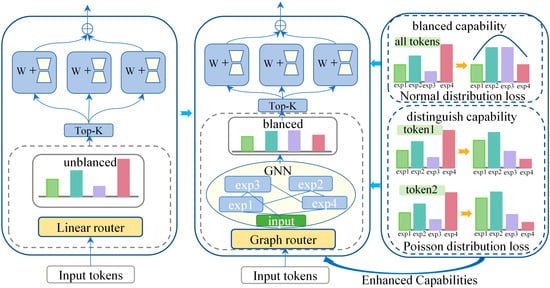
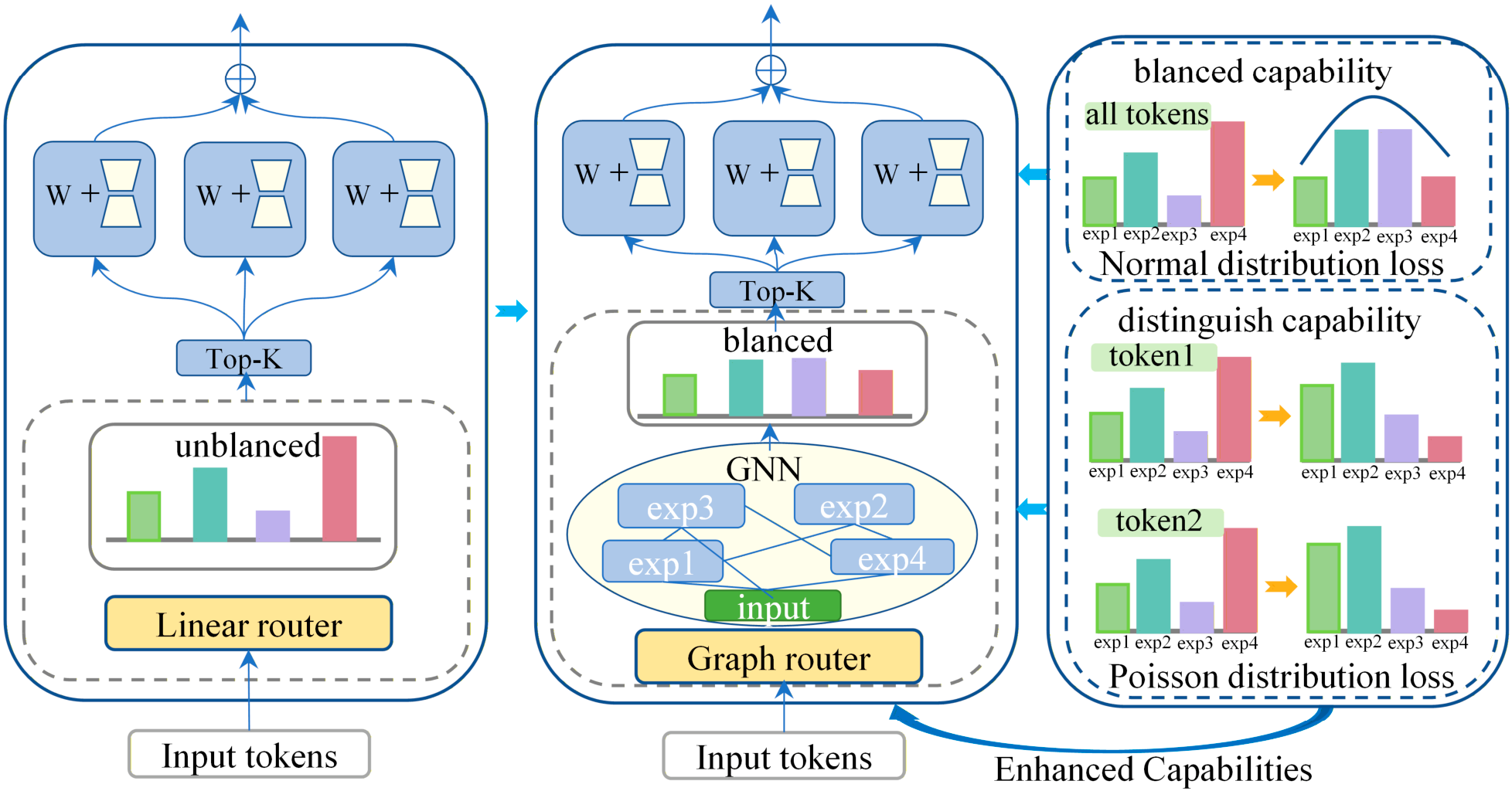
A Gated Mixture of Experts (GMoE) model was used to jointly predict the contamination classes of As, Cu, Hg and Cd (Figure 1) [23]. The model comprises multiple expert subnetworks and a graph-based gating network. Each expert independently learns nonlinear representations from the environmental predictors, while the graph router models interactions among experts and adaptively assigns their contributions to each sample. In contrast to a standard MoE with independent routing scores, GMoE incorporates expert-collaboration, expert-distinction and load-balancing constraints to promote specialization while preventing persistent over-utilization of a small subset of experts. The selected Top-K expert outputs are aggregated to generate metal-specific predictions. Details of the model architecture, routing procedure, loss functions, and regularization strategies are provided in Supplementary Methods S2. Expert-routing behaviour was evaluated using selected rates, Top-1 assignment rates, effective expert number, model-level expert utilization, and the Gini coefficient of expert loads.
Figure 1.
Structure of the graph-based mixture-of-experts (GMoE) model for soil heavy metal pollution prediction. Abbreviations: GMoE, graph-based mixture-of-experts; GNN, graph neural network; MLP, multilayer perceptron; KL, Kullback–Leibler divergence; Top-K, top-k expert selection.
2.4.2. Spatially Independent Validation Strategy
Soil heavy metal concentrations and environmental covariates are spatially structured, and nearby samples often share similar pedological, climatic, topographic and anthropogenic conditions. Consequently, a purely random train-test split may assign geographically adjacent samples to both subsets, allowing spatial autocorrelation to inflate apparent model performance. To reduce this source of information leakage and to assess the ability of the model to generalize to previously unseen regions, we adopted a spatial block hold-out validation strategy. Specifically, the study area was partitioned into regular 1° × 1° geographic blocks defined on a longitude-latitude grid. Each sample was assigned to a spatial block according to its coordinates, and data partitioning was then conducted at the block level rather than at the individual-sample level. All samples within the same block were assigned exclusively to either the training set or the test set. In this study, 70% of the spatial blocks were used for model training, whereas the remaining 30% were reserved as an independent spatial test set. This configuration was chosen to reduce spatial leakage while maintaining sufficient sample coverage for robust model fitting and evaluation at the European scale. We acknowledge that alternative block sizes or partitioning schemes may yield different performance estimates, and this should be considered when interpreting the validation results.
2.4.3. Geodetector
Geodetector is a spatial statistical method used to quantitatively assess the explanatory power of environmental factors on a target variable. It is particularly suitable for spatially stratified or gridded data and has been widely applied in public health [49], ecology [50], and environmental studies [51].
The model consists of four components: factor detection, interaction detection, ecological detection, and risk detection. In this study, we employed the Geodetector model to identify the driving factors controlling the spatial heterogeneity of soil heavy metal concentrations. The factor detection module is formulated as follows:
where , a higher value indicates a stronger explanatory power of the factor for the spatial variation in the dependent variable. In Equation (1), and represent the number of samples and the variance within stratum , respectively, while and denote the total sample size and variance across the entire study area.
3. Results
3.1. Contamination Concentration Patterns
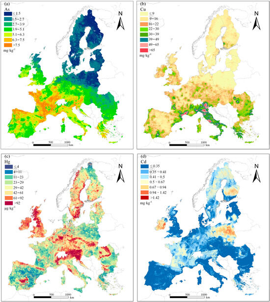
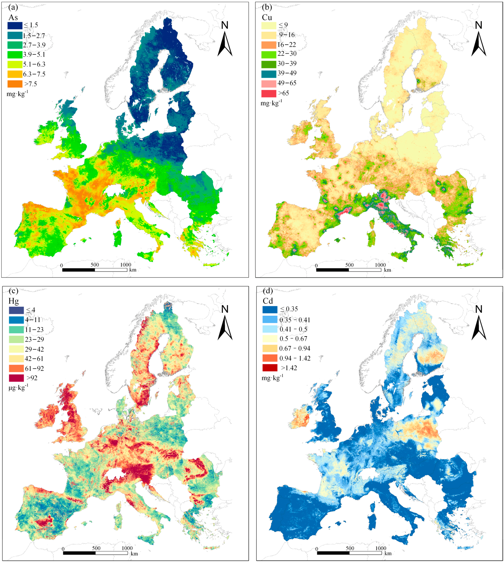
The spatial distribution of As in European topsoils showed a clear north–south gradient, with lower concentrations mainly distributed across Scandinavia and the Baltic region and higher concentrations occurring in parts of Southern and Western Europe (Figure 2a). Most northern areas were classified into the lowest As concentration classes, whereas Central and Western Europe were dominated by intermediate classes. Areas exceeding 7.5 mg kg−1 were mainly localized in southern and western regions. The class-frequency distribution further confirmed that As samples were distributed across several low-to-moderate classes (Supplementary Figure S1a). The corresponding continuous concentration-frequency distribution showed a broad, partly bimodal pattern, mainly within the low-to-moderate range and with a long upper tail reaching 64.64 mg kg−1 (Supplementary Figure S2a and Table S2).
Figure 2.
Spatial distribution of soil heavy metal concentrations in European topsoils. (a) As, (b) Cu, (c) Hg and (d) Cd. Concentration classes follow the classification thresholds used for model labelling and spatial visualization.
Cu concentrations displayed stronger spatial heterogeneity and a clearer southward increase than As (Figure 2b). Low Cu concentrations were mainly observed in Northern Europe and northern parts of Central Europe, whereas higher values occurred in southern Germany, Austria, the Czech Republic, Italy, southern France, and parts of Romania. Several mountainous and southern regions exceeded 65 mg kg−1. The class-frequency distribution showed that most Cu samples occurred in the lower concentration classes, with progressively fewer observations in high-concentration classes (Supplementary Figure S1b). The continuous concentration-frequency distribution was unimodal and positively skewed, and the mean Cu concentration was higher than the median, indicating the influence of localized high-value areas (Supplementary Figure S2b and Table S2).
Hg showed the strongest localized clustering among the four metals (Figure 2c). High-concentration areas were concentrated in the Central-Western European industrial corridor, Great Britain, the Alpine fringe, and parts of Scandinavia. This pattern suggests that Hg distribution is less zonal than Cu and more strongly shaped by localized enrichment. The class-frequency distribution showed a substantial proportion of samples in intermediate-to-high Hg classes compared with the other metals (Supplementary Figure S1c). The continuous concentration-frequency distribution was strongly right-skewed, with most observations occurring at low-to-intermediate concentrations and a pronounced tail toward high values. The mean Hg concentration was 47.74 μg kg−1, higher than the median of 36.59 μg kg−1, confirming the influence of high-concentration outliers (Supplementary Figure S2c and Table S2).
Cd concentrations were characterized by extensive low-background areas and discrete enrichment zones (Figure 2d). Most of the Iberian Peninsula, the United Kingdom, Italy, Hungary, and Romania fell within the lowest Cd classes, whereas elevated concentrations were mainly observed in central and eastern Ireland, Poland, and Finland. The class-frequency distribution was dominated by the lowest Cd class, indicating that high-Cd observations were comparatively rare (Supplementary Figure S1d). The continuous concentration-frequency distribution also showed a dominant low-concentration range with a positive tail toward higher concentrations. Compared with Cu and Hg, the smaller difference between the Cd mean and median indicates a more spatially constrained distribution with fewer extreme outliers (Supplementary Figure S2d and Table S2).
3.2. Performance of the GMoE in Soil Heavy Metal Prediction
3.2.1. Experimental Setup and Baseline Models
To rigorously evaluate the effectiveness of GMoE in soil heavy metal contamination classification, we compared its performance with two expert-based baseline models: a standard MoE and a multi-gate mixture-of-experts (MMoE). The standard MoE was used to assess the effect of introducing expert-based routing relative to a shared gating structure, whereas MMoE provided a stronger multi-task baseline with task-specific gates. To ensure a fair comparison, MoE, MMoE and GMoE used the same number of experts, and each expert adopted an identical multilayer perceptron (MLP) architecture with hidden layers of 256 and 128 units. All models were trained under the same data partitions, training protocols and early-stopping criteria. This experimental design allowed the performance gains of GMoE to be attributed more directly to its graph-guided routing and expert-collaboration mechanisms.
3.2.2. Evaluation Metrics
In this study, model performance was quantified using Accuracy, Weighted F1-score, and Macro F1-score. Accuracy was first used to provide an intuitive measure of the model’s overall predictive capability and is defined in Equation (2) as the proportion of correctly classified samples across all categories.
To further assess class-level performance, macro-precision and macro-recall were calculated as shown in Equations (3) and (4), respectively.
Based on these two quantities, the macro-F1-score was calculated according to Equation (5).
In Equations (2)–(5), K denotes the total number of classes, , and represent the true positives, false positives, and false negatives for class k, respectively. Unlike global metrics that aggregate all predictions first, Macro F1 computes precision and recall for each class individually, then averages these values across all classes.
For a more practical evaluation under class-imbalanced conditions, weighted precision and weighted recall were further calculated as shown in Equations (6) and (7), respectively. The weighted F1-score was then calculated according to Equation (8). In Equations (6)–(8), n_k denotes the number of samples in class k, and N is the total number of samples. By weighting each class’s contribution according to its sample proportion, the weighted F1-score complements the macro-F1-score and provides a more realistic assessment of model performance under skewed class distributions.
3.2.3. Model Performance Under Spatial-Block Validation
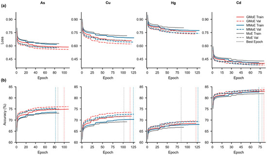
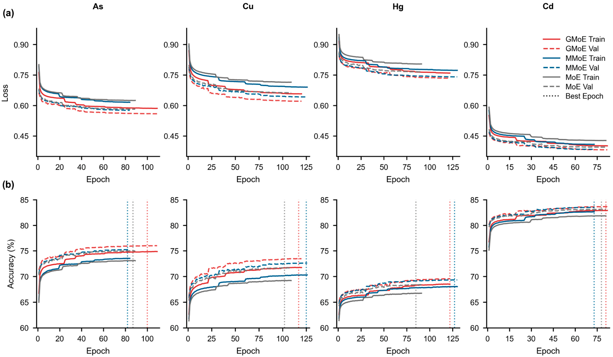
GMoE, MMoE and MoE were evaluated under identical training protocols. All models were trained for a maximum of 300 epochs with early stopping, and all tasks reached their optimal validation performance within 120 epochs (Figure 3; Table 2). For visualization, the metal-specific loss and accuracy curves were truncated at the corresponding best-validation epoch, as indicated by the vertical dashed lines in Figure 3.
Figure 3.
Training and validation loss (a) and accuracy (b) curves of GMoE, MMoE, and MoE models for soil As, Cu, Hg, and Cd prediction. Vertical dashed lines represent the optimal epochs corresponding to the best validation accuracy.
Table 2.
Classification performance of GMoE, MMoE, and MoE models for soil heavy metal prediction.
The learning curves revealed clear differences in training stability among the three models (Figure 3). Across the four prediction tasks, GMoE generally showed more stable convergence, with lower validation loss and higher validation accuracy after convergence than MMoE and MoE. The clearest separation from the baseline models was observed for As and Cu. These patterns indicate that graph-based expert routing improved both optimization stability and validation performance.
The classification metrics further demonstrated that GMoE achieved the strongest overall performance across the four metals (Table 2). For As, GMoE reached an accuracy of 76.96%, exceeding MMoE and MoE by 4.79 and 5.00 percentage points, respectively. Its macro-F1 reached 0.73, compared with 0.63 for both baselines, indicating improved recognition across contamination classes rather than improvement driven only by dominant classes. For Cu, GMoE also achieved the highest accuracy and macro-F1, reaching 75.43% and 0.64, respectively, compared with 72.57% and 0.60 for MMoE and 71.66% and 0.59 for MoE.
Performance differences were smaller for Hg and Cd. For Hg, GMoE achieved the highest accuracy and macro-F1, although its advantage over MMoE was limited. For Cd, the three models produced similar weighted-F1 and weighted-precision values, whereas GMoE retained the highest accuracy and macro-F1. These smaller gains indicate that the benefits of GMoE varied among metals, but its consistent macro-F1 advantage suggests improved class-balanced prediction across all four tasks.
The optimal epochs also differed among models and metals. MMoE reached its optimal performance earlier than GMoE for As and Cd, whereas GMoE reached its optimal epoch earlier than MMoE for Cu and Hg (Figure 3; Table 2). MoE reached its optimal epoch earliest for Cu and Hg but produced lower final classification metrics. Thus, earlier convergence did not necessarily correspond to stronger predictive performance. Overall, GMoE provided the most consistent balance between training stability, overall accuracy and class-balanced prediction. Its expert-routing behaviour is examined in Section 3.2.4. A brief comparison of training time across the three expert-based models is provided in Table 3. Under the current experimental settings, GMoE required less training time than MMoE on average, but more than MoE. These results suggest that the performance gains of GMoE were achieved with a moderate computational cost relative to the two comparison models.
Table 3.
Approximate training time(s) of the three expert-based models across the four target metals.
3.2.4. Expert Routing Behaviour and Spatial Gate-Weight Allocation
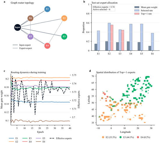
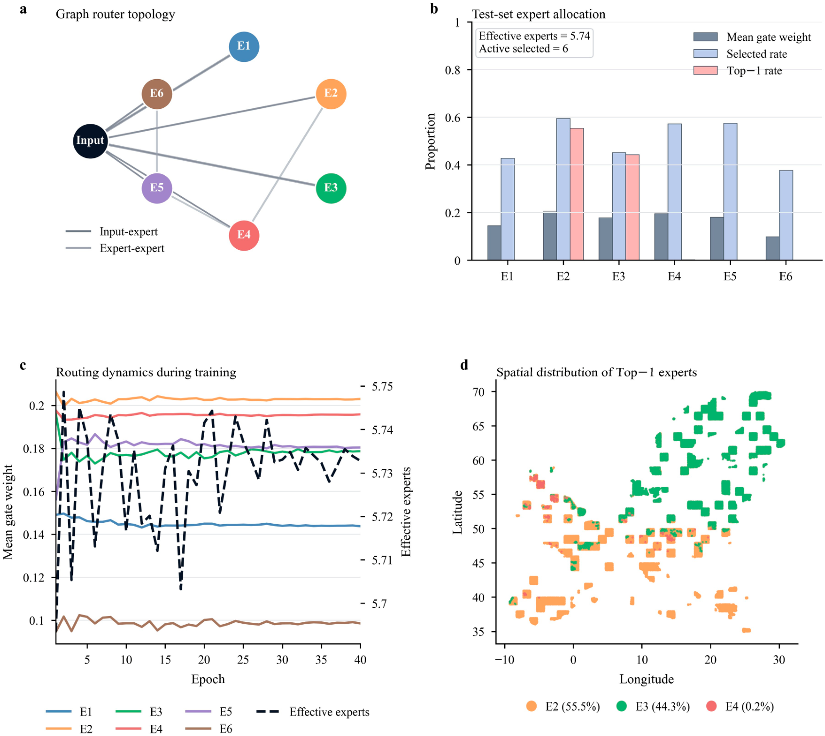
The GMoE router maintained broad expert participation on the spatially independent test set rather than collapsing to a single expert [23]. The graph router connected the input node with all six experts and retained sparse expert-expert links, indicating that routing decisions were informed by both sample features and inter-expert relationships (Figure 4a). Across 707,386 test samples, all six experts were activated in the Top-K routing process, with an effective expert number of 5.74. Expert selection rates ranged from 37.7% for E6 to 59.5% for E2, showing that each expert contributed to the final prediction ensemble after sparse routing (Figure 4b; Table 4).
Figure 4.
Expert routing behaviour of the GMoE model. (a) Graph topology used by the router, including input-expert and expert-expert connections. (b) Test-set expert allocation summarized by mean gate weight, selected rate, and Top-1 rate. (c) Temporal dynamics of expert gate weights and effective expert number during training. (d) Spatial distribution of the Top-1 expert assigned to each test sample. The Top-1 map shows only the dominant expert for each sample and does not represent the full Top-K expert contribution.
Table 4.
Test-set expert allocation summary for the GMoE model.
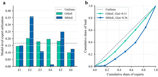
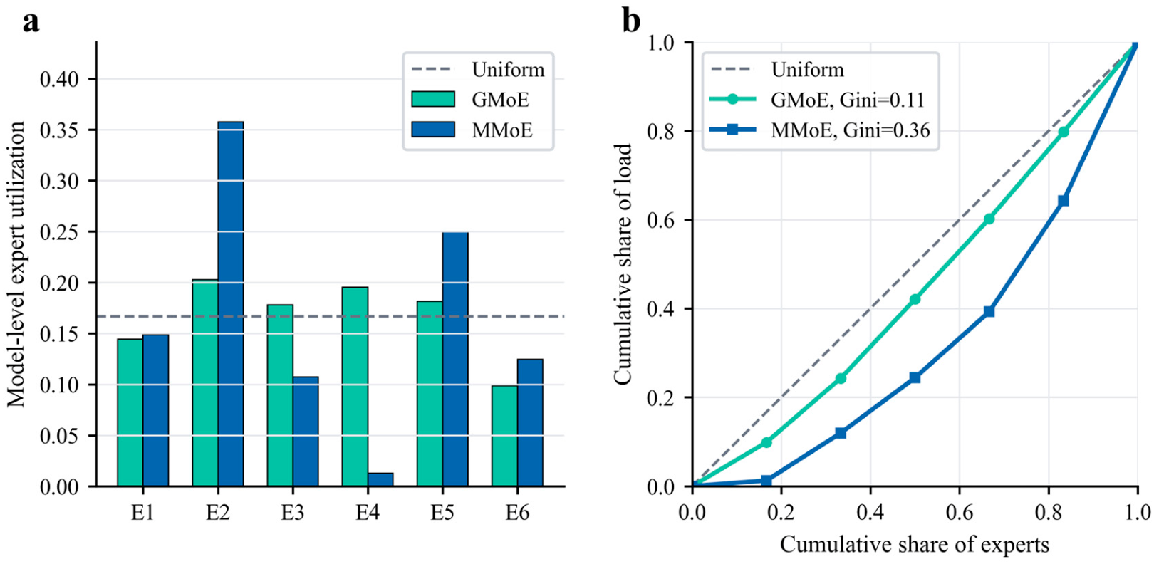
Expert utilization was further compared between GMoE and MMoE. Aggregated expert loads and Lorenz curves were used for this comparison. GMoE showed a flatter expert-utilization distribution that was closer to the uniform reference line, whereas MMoE concentrated more load on a limited subset of experts (Figure 5a). The lower Gini coefficient of GMoE further indicates weaker expert-load concentration and more balanced routing (Figure 5b).
Figure 5.
Comparison of expert utilization and load concentration between GMoE and MMoE. (a) Aggregated model-level expert utilization. The dashed line indicates uniform expert utilization. (b) Lorenz curves of expert-load concentration. Curves closer to the diagonal line indicate more balanced expert allocation, and lower Gini coefficients indicate weaker load concentration.
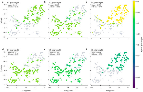
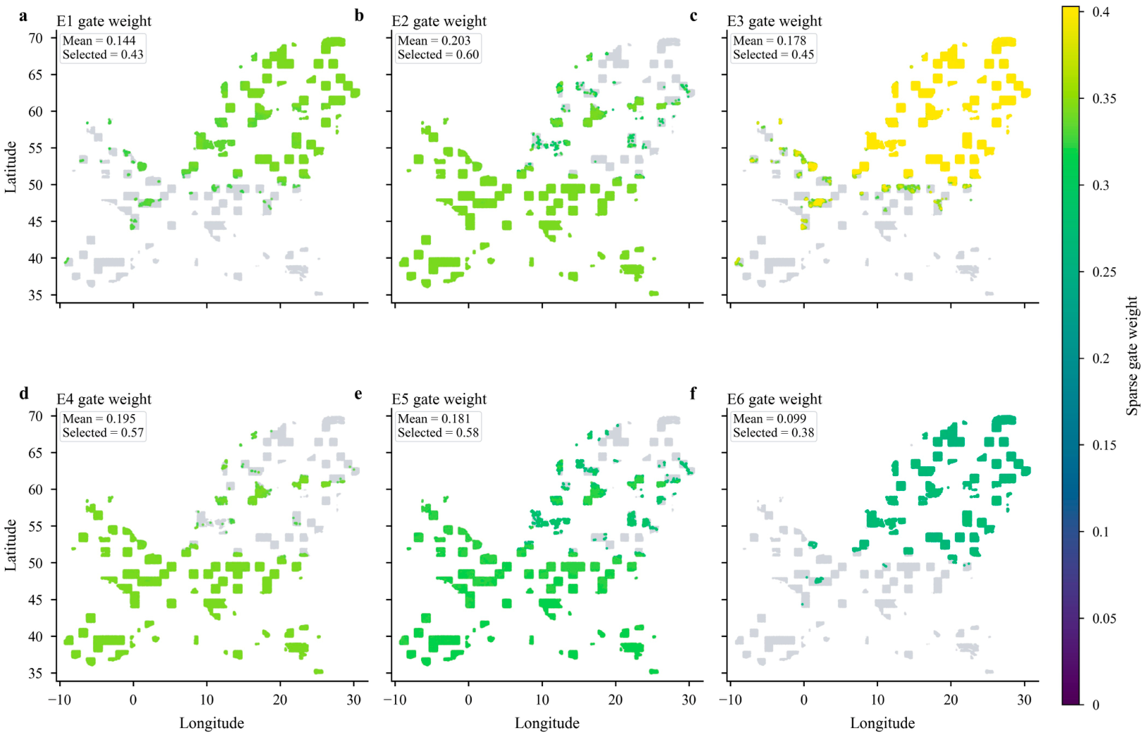
The Top-1 routing assignments were more spatially concentrated than the overall Top-K selection. E2 and E3 dominated the primary routing decisions, accounting for 55.4% and 44.4% of test samples, respectively, whereas E4 was assigned as the top expert for only 0.24% of samples. E1, E5 and E6 were not selected as Top-1 experts, but they remained active as secondary experts in the Top-K set. The sparse gate-weight maps further confirmed these auxiliary contributions, showing that non-dominant experts were still selected for geographically structured subsets of samples with varying gate weights (Figure 6). Thus, the router did not perform a simple hard partition of the study area, but combined dominant regional experts with auxiliary expert contributions.
Figure 6.
Spatial distribution of sparse gate weights for each GMoE expert. Grey points indicate samples not selected by the Top-K router, and coloured points indicate selected samples, with colour intensity representing the sparse gate weight. (a) E1; (b) E2; (c) E3; (d) E4; (e) E5; and (f) E6. This figure complements the top-1 expert map in the main text by showing auxiliary contributions from non-dominant experts.
Routing behaviour was also stable during model training. Over 40 epochs, the effective number of experts remained high, ranging from 5.69 to 5.75, and the mean gate weights of individual experts changed only modestly after the early training stage (Figure 4c). E2 and E4 maintained relatively high mean gate weights, whereas E6 had a lower average weight but was still selected for more than one-third of test samples. These results indicate that the load-balancing and expert-distinction constraints maintained differentiated expert roles while avoiding severe expert under-utilization.
Spatially, Top-1 expert allocation showed clear geographic structure (Figure 4d). E2 was mainly assigned to southern, western and central European test samples, whereas E3 dominated northern and north-eastern regions. E4 appeared only in scattered local areas. This spatial organization indicates that the GMoE router captured region-dependent prediction regimes.
3.3. Analysis of the Driving Factors of Soil Heavy Metal Pollution
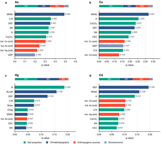
The Geodetector model was employed to quantify the explanatory power (q values) of environmental, soil, socioeconomic, and anthropogenic factors on the spatial differentiation of soil heavy metal concentrations (As, Cu, Hg, and Cd; Figure 7). The q value represents the explanatory power of each factor for the spatially stratified heterogeneity of heavy metal concentrations, with higher values indicating stronger spatial association with the target metal.
Figure 7.
Dominant factors influencing the spatial distribution of soil heavy metals derived from the Geodetector model. (a) As; (b) Cu; (c) Hg; and (d) Cd. The q value represents the explanatory power of each factor on the spatial variability of heavy metal concentrations.
For As (Figure 7a), SRAD showed the highest explanatory power (q = 0.490), followed by the C:N ratio (q = 0.356) and DEF (q = 0.351). Soil properties also featured prominently in the factor ranking, with silt content (q = 0.335), K (q = 0.334) and CaCO3 (q = 0.310) among the strongest associations. Anthropogenic-source variables remained important, particularly industrial Cu emissions to soil (q = 0.304) and industrial As emissions to soil (q = 0.244). Overall, these results indicated that the spatial heterogeneity of As was associated with both soil-related controls and anthropogenic inputs.
For Cu (Figure 7b), SRAD again showed the highest explanatory power (q = 0.321), followed by K (q = 0.255), CaCO3 (q = 0.237), DEF (q = 0.230) and silt content (q = 0.226). Soil-related variables were also prominent in the factor ranking, whereas climate and topographic variables showed comparatively weaker associations. Overall, these results indicated that the spatial distribution of Cu was associated with both climatic gradients and soil physicochemical properties, with additional contributions from anthropogenic sources.
For Hg (Figure 7c), the overall q values were lower than those for As and Cu. N was identified as the strongest individual driver (q = 0.188), followed by runoff (q = 0.158), DEF (q = 0.124), C:N ratio (q = 0.073), and slope (q = 0.072). At the category level, soil properties and climate/topography showed nearly equal contributions, accounting for 41.1% and 41.7% of the summed explanatory contribution, respectively. In contrast, anthropogenic-source and socioeconomic variables contributed relatively little, accounting for 14.5% and 2.6%, respectively.
For Cd (Figure 7d), DEF (q = 0.195) and SRAD (q = 0.158) were the principal determinants, followed by K (q = 0.141). Unlike Hg, Cd showed a stronger contribution from anthropogenic-source variables, which accounted for 31.5% of the summed explanatory contribution. In particular, industrial Cd emissions to soil (Ind. Cd (Soil), q = 0.104), industrial As emissions to soil (q = 0.103), and industrial Hg emissions to soil (q = 0.080) showed relatively high explanatory power, indicating that Cd spatial heterogeneity was influenced by both climatic regulation and industrial-source signals.
4. Discussion
4.1. Spatially Robust Prediction Under Spatial-Block Validation
Many machine-learning studies of soil heavy metal contamination evaluate model performance using random sample splitting, including studies conducted over spatially extensive regions [27,52]. Although convenient, random splitting can place neighbouring samples with similar soil properties, environmental conditions and contamination sources in both training and testing sets. Reported performance may therefore primarily represent interpolation within sampled regions rather than prediction in geographically independent areas. This issue is particularly important for continental-scale soil datasets, where strong spatial autocorrelation can produce overly optimistic accuracy estimates [25,26,27]. The spatial-block hold-out strategy used here provided a more conservative assessment by separating training and test samples geographically. Under this stricter evaluation, GMoE consistently outperformed MoE and MMoE across all four metals, with the clearest gains for As and Cu (Table 2). This result indicates that graph-based expert routing retained predictive value beyond spatially clustered neighbourhoods and was not solely dependent on local similarities between training and test samples. The smaller gains for Hg and Cd suggest that expert-based modelling cannot fully resolve contamination patterns dominated by localized enrichment, class imbalance and complex transport processes [36,53].
4.2. Element-Specific Driving Mechanisms
For As, SRAD, C:N ratio and DEF were the three strongest explanatory factors (Figure 7a), suggesting that As spatial heterogeneity was mainly associated with regional hydroclimatic gradients and soil biogeochemical conditions [7,54]. The association with SRAD may reflect regional variations in evapotranspiration, soil moisture, redox conditions and weathering intensity, rather than a direct radiation effect, because As mobility is strongly influenced by hydrological and redox conditions [54,55,56].
These conditions can regulate As mobility by affecting microbial activity, oxygen availability and the stability of Fe/Mn (hydr)oxides that retain sorbed As [54,56]. The contribution of C:N ratio may reflect the role of organic matter and nutrient cycling in As retention and release, as organic compounds and competing ligands can alter As adsorption, complexation and desorption processes [56,57,58,59]. Meanwhile, As species can be transported through leaching, runoff and groundwater flow [56,60]. Although pH was not retained in the final factor set because of multicollinearity, its effect may be partly represented by CaCO3 and related soil properties. The explanatory power of CaCO3 and silt suggests that carbonate buffering, soil texture and mineral-associated adsorption contributed to the spatial differentiation of As [54,57,61].
For Cu, Solar radiation and climatic water deficit (DEF) showed relatively strong explanatory power (Figure 7b). Higher precipitation combined with relatively warm conditions may be associated with increased Cu accumulation because agricultural systems under humid climates tend to require more frequent fungicide applications [17,18,62]. For example, vineyards in northern Italy experience more frequent antifungal treatments and consequently exhibit higher Cu concentrations compared with drier southern regions [63], consistent with our findings. This interpretation is consistent with the relatively strong explanatory power of land cover and the reported association between agricultural management and soil Cu accumulation [64,65,66]. In addition, the strong explanatory power of K for As and Cu may reflect the abundance of 2:1 clay minerals and their associated metal-retention capacity [65].
For Hg, N showed the highest explanatory power (Figure 7c), which may reflect the strong affinity of Hg for soil organic matter (SOM). This is consistent with previous studies showing that soil organic matter can act as both a reservoir and a transport medium for Hg, facilitating its retention and downward migration in organic-rich soils [67,68,69,70]. The relatively high explanatory power of runoff and DEF suggests that hydroclimatic conditions may influence Hg redistribution at continental scales [71,72]. Likewise, the contribution of slope indicates that topography-mediated transport may also be important [73].
For Cd, DEF showed the strongest explanatory power, followed by SRAD and K (Figure 7d), suggesting that Cd spatial heterogeneity was closely associated with regional water balance, hydroclimatic gradients and soil-related controls. This is consistent with European-scale studies showing that Cd patterns are jointly shaped by geology, weathering, soil formation, climate, pH, clay content, organic matter, topography, erosion and leaching processes [36]. DEF and SRAD may influence Cd mobility and accumulation by regulating soil moisture, evapotranspiration and leaching intensity, while soil pH, organic matter, clay minerals and hydrous oxides are known to affect Cd sorption–desorption, solubility and transport [66,68]. K may partly reflect fertilization history, because long-term fertilizer inputs, especially phosphate fertilizers, can introduce Cd into agricultural soils and modify Cd availability through changes in soil chemistry [74]. Although pH was not retained in the final factor set because of multicollinearity, its effect may be partly represented by correlated variables such as CaCO3, CEC, C:N ratio and texture-related properties [75].
Across the four metals, industrial-source variables contributed to spatial heterogeneity but ranked among the factors most strongly associated with the observed spatial patterns. Hydroclimatic and soil-related factors showed stronger associations for Hg and Cd, suggesting that environmental transport and retention may have played important roles in shaping their spatial patterns [67,68,69]. As showed a stronger association with anthropogenic indicators, potentially reflecting persistent inputs from mining, smelting and combustion [76,77]. Thus, European topsoil contamination appears to reflect the combined effects of source inputs and environmental filtering.
4.3. Expert Routing and Load-Balancing Behaviour
Expert-based architectures can better accommodate spatial heterogeneity by allowing different subnetworks to learn distinct predictor–contamination relationships [19,21]. However, conventional MoE and MMoE architectures may repeatedly select a small expert subset, reducing effective model capacity [22]. GMoE addresses this limitation by combining graph-based expert collaboration with distinction and load-balancing constraints [23]. Under spatial-block validation, GMoE outperformed both MoE and MMoE across all four metals (Table 2). All six experts participated in Top-K aggregation, and the effective expert number reached 5.737, indicating that routing did not collapse onto a single expert (Figure 4; Table 4). Expert utilization was nevertheless differentiated: E2 and E3 dominated Top-1 assignments, whereas the remaining experts mainly provided secondary contributions (Figure 4). Compared with MMoE, GMoE also showed a more balanced model-level expert utilization pattern, with a lower Gini coefficient of expert loads (Figure 5). Thus, load balancing preserved broad expert participation without enforcing uniform routing, allowing the model to retain dominant and complementary prediction pathways.
4.4. Limitations and Uncertainties
Model evaluation may remain sensitive to spatial-block size and residual spatial dependence. Differences in the temporal coverage, spatial resolution and uncertainty of the integrated datasets may also affect the interpretation of source-environment relationships. In addition, we did not generate spatial uncertainty maps or repeat the spatial hold-out validation across multiple alternative partitions, which limits the assessment of predictive uncertainty and stability. The relatively low macro-F1 for Hg further indicates that localized enrichment and class imbalance continue to constrain the prediction of high-contamination classes. Geodetector identifies spatial associations rather than causal relationships, and highly ranked variables may represent correlated environmental processes rather than direct mechanisms. The analysis was also limited to total topsoil concentrations and did not consider metal speciation, bioavailability or vertical profiles. Future studies integrating temporally consistent predictors, improved source inventories and process-relevant soil observations could further strengthen both prediction and interpretation.
5. Conclusions
This study assessed As, Cu, Hg and Cd contamination in European topsoils by integrating spatially validated multi-metal prediction with driver attribution. Under spatial-block validation, GMoE produced more reliable predictions than MMoE and MoE, with the clearest improvements for As and Cu. Routing analysis showed that the model maintained broad and balanced expert participation, suggesting that its predictive capacity was not concentrated in only a few experts. The attribution results revealed that continental-scale contamination patterns were controlled by both environmental filtering and source-related inputs. Soil properties and hydroclimatic conditions explained much of the spatial variation, while anthropogenic-source signals were more evident for As and Cd. These results highlight the need to combine spatially robust prediction with environmental interpretation in large-scale soil contamination assessment, and provide useful support for regional risk prioritization and targeted pollution management.
Supplementary Materials
The following supporting information can be downloaded at: https://www.mdpi.com/article/10.3390/app16147272/s1, Figure S1: Frequency distributions of As, Cu, Hg, and Cd concentration classes in European topsoils; Figure S2: Continuous concentration distributions of As, Cu, Hg, and Cd in European topsoils; Table S1: Predictors removed during variance inflation factor (VIF) screening; Table S2: Descriptive statistics of soil heavy metal concentrations in the cleaned modelling dataset.
Author Contributions
L.N.: Conceptualization, Methodology, Validation, Formal analysis, Data curation, Visualization, Writing—original draft, Writing—review and editing. Y.Z. (Yongzhang Zhou): Supervision, Resources, Project administration, Funding acquisition, Writing—review and editing. B.Z.: Methodology, Writing—review and editing. C.S.: Formal analysis, Visualization. Y.Z. (Yuqing Zhang): Conceptualization, Methodology, Formal analysis, Visualization, Writing—review and editing. All authors have read and agreed to the published version of the manuscript.
Funding
This research was funded by the National Key Research and Development Plan, grant number 2022YFF0801201; the GuangXi Key Areas Research and Development Project, grant number AB24010156; the National Natural Science Foundation of China, grant number U1911202; and the Inner Mongolia Autonomous Region “Jiebang Guashuai” Project, grant number 2025KJTW0020.
Data Availability Statement
The publicly shareable processed data and code associated with this study are available at https://doi.org/10.17632/29tgfxzmk9.1. Raw LUCAS point-level soil observations and third-party source datasets are not redistributed because they are subject to the original data providers’ access and licence conditions. These source datasets should be accessed through their respective providers as described in the manuscript.
Conflicts of Interest
The authors declare no conflicts of interest.
References
- Chen, H.; Teng, Y.; Lu, S.; Wang, Y.; Wang, J. Contamination features and health risk of soil heavy metals in China. Sci. Total Environ. 2015, 512–513, 143–153. [Google Scholar] [CrossRef] [Scilit] [PubMed]
- Liu, Y.; van der Heijden, M.G.A.; Riedo, J.; Sanz-Lazaro, C.; Eldridge, D.J.; Bastida, F.; Moreno-Jiménez, E.; Zhou, X.; Hu, H.; He, J.; et al. Soil contamination in nearby natural areas mirrors that in urban greenspaces worldwide. Nat. Commun. 2023, 14, 1706. [Google Scholar] [CrossRef] [Scilit] [PubMed]
- Zhang, H.; Zhao, B.; Song, Y.; Yang, Y.; Cai, L.; Miao, Q.; Jiang, T. Soil contamination in contaminated sites with key standards: A global analysis and perspective. J. Hazard. Mater. 2025, 494, 138724. [Google Scholar] [CrossRef] [Scilit] [PubMed]
- Binner, H.; Sullivan, T.; Jansen, M.A.K.; McNamara, M.E. Metals in urban soils of Europe: A systematic review. Sci. Total Environ. 2023, 854, 158734. [Google Scholar] [CrossRef] [Scilit] [PubMed]
- Hou, D.; Jia, X.; Wang, L.; McGrath, S.P.; Zhu, Y.; Hu, Q.; Zhao, F.; Bank, M.S.; O’Connor, D.; Nriagu, J. Global soil pollution by toxic metals threatens agriculture and human health. Science 2025, 388, 316–321. [Google Scholar] [CrossRef] [Scilit] [PubMed]
- Qi, C.; Hu, T.; Zheng, Y.; Wu, M.; Tang, F.H.M.; Liu, M.; Zhang, B.; Derrible, S.; Chen, Q.; Hu, G.; et al. Global and regional patterns of soil metal(loid) mobility and associated risks. Nat. Commun. 2025, 16, 2947. [Google Scholar] [CrossRef] [Scilit] [PubMed]
- Fendrich, A.N.; Van Eynde, E.; Stasinopoulos, D.M.; Rigby, R.A.; Mezquita, F.Y.; Panagos, P. Modeling arsenic in European topsoils with a coupled semiparametric (GAMLSS-RF) model for censored data. Environ. Int. 2024, 185, 108544. [Google Scholar] [CrossRef] [Scilit] [PubMed]
- Li, J.; Li, X.; Wang, C.; Liu, J.; Gao, Z.; Li, K.; Tuo, X.; Zang, F. Pollution characteristics and probabilistic risk assessment of heavy metal(loid)s in agricultural soils across the Yellow River Basin, China. Ecol. Indic. 2024, 167, 112676. [Google Scholar] [CrossRef] [Scilit]
- Zhang, L.; Yang, L.; Ma, Y.; Zhu, A.; Wei, R.; Liu, J.; Greve, M.H.; Zhou, C. Regional-scale soil carbon predictions can be enhanced by transferring global-scale soil–environment relationships. Geoderma 2025, 461, 117466. [Google Scholar] [CrossRef] [Scilit]
- Yang, B.; He, A.; Ren, Z.; Yu, K.; Zhao, G.; Fan, Y.; Wang, Q.; Luo, S. A transfer learning–enhanced deep learning framework for efficient and interpretable soil heavy metal pollution prediction under data scarcity and spatial heterogeneity. J. Hazard. Mater. 2025, 495, 138926. [Google Scholar] [CrossRef] [Scilit] [PubMed]
- Lv, S.; Zhu, Y.; Cheng, L.; Zhang, J.; Shen, W.; Li, X. Evaluation of the prediction effectiveness for geochemical mapping using machine learning methods: A case study from northern Guangdong Province in China. Sci. Total Environ. 2024, 927, 172223. [Google Scholar] [CrossRef] [Scilit] [PubMed]
- Shi, T.; Zhang, J.; Shen, W.; Wang, J.; Li, X. Machine learning can identify the sources of heavy metals in agricultural soil: A case study in northern Guangdong Province, China. Ecotoxicol. Environ. Saf. 2022, 245, 114107. [Google Scholar] [CrossRef] [Scilit] [PubMed]
- Zhao, W.; Ma, J.; Liu, Q.; Dou, L.; Qu, Y.; Shi, H.; Sun, Y.; Chen, H.; Tian, Y.; Wu, F. Accurate Prediction of Soil Heavy Metal Pollution Using an Improved Machine Learning Method: A Case Study in the Pearl River Delta, China. Environ. Sci. Technol. 2023, 57, 17751–17761. [Google Scholar] [CrossRef] [Scilit] [PubMed]
- Wang, M.; Zhao, W.; Wu, X.; Yang, A.; Chen, Y.; Qu, Y.; Ma, J.; Wu, F. Advanced three-dimensional prediction model based on stable machine learning for soil pollution: A case study from a contaminated site in Southern China. J. Hazard. Mater. 2025, 494, 138561. [Google Scholar] [CrossRef] [Scilit] [PubMed]
- Salgado, L.; López-Sánchez, C.A.; Colina, A.; Baragaño, D.; Forján, R.; Gallego, J.R. Hg and As pollution in the soil-plant system evaluated by combining multispectral UAV-RS, geochemical survey and machine learning. Environ. Pollut. 2023, 333, 122066. [Google Scholar] [CrossRef] [Scilit] [PubMed]
- Wu, Y.; Liu, Q.; Ma, J.; Zhao, W.; Chen, H.; Qu, Y. Antimony, beryllium, cobalt, and vanadium in urban park soils in Beijing: Machine learning-based source identification and health risk-based soil environmental criteria. Environ. Pollut. 2022, 293, 118554. [Google Scholar] [CrossRef] [Scilit] [PubMed]
- Barkhordari, M.S.; Qi, C. Prediction of zinc, cadmium, and arsenic in european soils using multi-end machine learning models. J. Hazard. Mater. 2025, 490, 137800. [Google Scholar] [CrossRef] [Scilit] [PubMed]
- Zhang, Y.; Yang, Q. A Survey on Multi-Task Learning. IEEE Trans. Knowl. Data Eng. 2022, 34, 5586–5609. [Google Scholar] [CrossRef] [Scilit]
- Jacobs, R.A.; Jordan, M.I.; Nowlan, S.J.; Hinton, G.E. Adaptive Mixtures of Local Experts. Neural Comput. 1991, 3, 79–87. [Google Scholar] [CrossRef] [Scilit] [PubMed]
- Tang, H.; Liu, J.; Zhao, M.; Gong, X. Progressive Layered Extraction (PLE): A Novel Multi-Task Learning (MTL) Model for Personalized Recommendations. In Proceedings of the 14th ACM Conference on Recommender Systems; Association for Computing Machinery: New York, NY, USA, 2020; pp. 269–278. [Google Scholar]
- Lu, X.; Du, J.; Wang, G.; Li, X.; Sun, L.; Zheng, L.; Huang, X. Identifying multiple soil pollutions of potentially contaminated sites based on multi-gate mixture-of-experts network. Sci. Total Environ. 2023, 903, 166218. [Google Scholar] [CrossRef] [Scilit] [PubMed]
- Wang, X.; Zhang, M.; Zhou, Y.; Wang, L.; Zeng, L.; Cui, Y.; Sun, X. Simultaneous estimation of multiple soil properties from vis-NIR spectra using a multi-gate mixture-of-experts with data augmentation. Geoderma 2025, 453, 117127. [Google Scholar] [CrossRef] [Scilit]
- Bai, T.; Yu, Y.; Huang, L.; Xu, Z.; Zhao, Z.; Shi, C. GMoE: Empowering LLMs Fine-Tuning via MoE Graph Collaboration. arXiv 2024, arXiv:2412.16216. [Google Scholar]
- Sun, M.; Liu, H.; Gong, P.; Dang, Y.; Li, P.; Meng, Q. A multi-task deep learning framework integrating land-use types for synchronous prediction of soil properties. Microchem. J. 2026, 225, 117912. [Google Scholar] [CrossRef] [Scilit]
- Meyer, H.; Pebesma, E. Predicting into unknown space? Estimating the area of applicability of spatial prediction models. Methods Ecol. Evol. 2021, 12, 1620–1633. [Google Scholar] [CrossRef] [Scilit]
- Roberts, D.R.; Bahn, V.; Ciuti, S.; Boyce, M.S.; Elith, J.; Guillera-Arroita, G.; Hauenstein, S.; Lahoz-Monfort, J.J.; Schröder, B.; Thuiller, W.; et al. Cross-validation strategies for data with temporal, spatial, hierarchical, or phylogenetic structure. Ecography 2017, 40, 913–929. [Google Scholar] [CrossRef] [Scilit]
- Schratz, P.; Muenchow, J.; Iturritxa, E.; Richter, J.; Brenning, A. Hyperparameter tuning and performance assessment of statistical and machine-learning algorithms using spatial data. Ecol. Model. 2019, 406, 109–120. [Google Scholar] [CrossRef] [Scilit]
- Valavi, R.; Elith, J.; Lahoz-Monfort, J.J.; Guillera-Arroita, G. BlockCV: An r package for generating spatially or environmentally separated folds for k-fold cross-validation of species distribution models. Methods Ecol. Evol. 2019, 10, 225–232. [Google Scholar]
- Han, F.; Deng, Y.; Liu, Q.; Zhou, Y.; Wang, J.; Huang, Y.; Zhang, Q.; Bian, J. Construction and application of the knowledge graph method in management of soil pollution in contaminated sites: A case study in South China. J. Environ. Manag. 2022, 319, 115685. [Google Scholar] [CrossRef] [Scilit]
- Ling, S.; Li, X.; Zhang, S.; Wei, W.; Liu, Z.; Feng, J.; Wang, J.; Sun, C.; Zhang, G. Machine and deep learning-driven geospatial prediction modelling of soil cadmium and nickel with pollution risk mapping underlaid by black shale in Qianjiang County, China. J. Hydrol. Reg. Stud. 2025, 62, 102857. [Google Scholar] [CrossRef] [Scilit]
- Zhao, W.; Ma, J.; Li, X.; Li, T.; Wang, M.; Chen, Y. Explainable deep learning unveils critical scenarios driving soil cadmium pollution in a coastal industrial city in China: A geospatial AI approach. Environ. Pollut. 2025, 382, 126769. [Google Scholar] [CrossRef] [Scilit] [PubMed]
- Kanji, S.; Das, S. Assessing predictability of spatio-temporal soil-moisture heterogeneity with satellite-data using GeoDetector and ensemble machine learning models considering environmental and climatic factors. J. Hydrol. 2025, 663, 134312. [Google Scholar] [CrossRef] [Scilit]
- Tegegne, A.M.; Lohani, T.K. Geodetector based statistical and machine learning approach for sustainable water resources within the gunabay watershed in the upper Blue Nile Basin, Ethiopia. Geosyst. Geoenviron. 2025, 4, 100424. [Google Scholar] [CrossRef] [Scilit]
- Zhu, M.; Yu, X.; Chen, K.; Tan, H.; Yuan, J. Spatiotemporal characteristics and driving factors of chemical oxygen demand emissions in China’s wastewater: An analysis based on spatial autocorrelation and geodetector. Ecol. Indic. 2024, 166, 112308. [Google Scholar] [CrossRef] [Scilit]
- Ballabio, C.; Panagos, P.; Lugato, E.; Huang, J.; Orgiazzi, A.; Jones, A.; Fernández-Ugalde, O.; Borrelli, P.; Montanarella, L. Copper distribution in European topsoils: An assessment based on LUCAS soil survey. Sci. Total Environ. 2018, 636, 282–298. [Google Scholar] [CrossRef] [Scilit] [PubMed]
- Ballabio, C.; Jones, A.; Panagos, P. Cadmium in topsoils of the European Union—An analysis based on LUCAS topsoil database. Sci. Total Environ. 2024, 912, 168710. [Google Scholar] [CrossRef] [Scilit] [PubMed]
- Panagos, P.; Jiskra, M.; Borrelli, P.; Liakos, L.; Ballabio, C. Mercury in European topsoils: Anthropogenic sources, stocks and fluxes. Environ. Res. 2021, 201, 111556. [Google Scholar] [CrossRef] [Scilit] [PubMed]
- Ballabio, C.; Panagos, P.; Monatanarella, L. Mapping topsoil physical properties at European scale using the LUCAS database. Geoderma 2016, 261, 110–123. [Google Scholar] [CrossRef] [Scilit]
- Ballabio, C.; Lugato, E.; Fernández-Ugalde, O.; Orgiazzi, A.; Jones, A.; Borrelli, P.; Montanarella, L.; Panagos, P. Mapping LUCAS topsoil chemical properties at European scale using Gaussian process regression. Geoderma 2019, 355, 113912. [Google Scholar] [CrossRef] [Scilit] [PubMed]
- Abatzoglou, J.T.; Dobrowski, S.Z.; Parks, S.A.; Hegewisch, K.C. TerraClimate, a high-resolution global dataset of monthly climate and climatic water balance from 1958–2015. Sci. Data 2018, 5, 170191. [Google Scholar] [CrossRef] [Scilit] [PubMed]
- European Environment Agency (EEA). European Pollutant Release and Transfer Register (E-PRTR); European Environment Agency: Copenhagen, Denmark, 2020; Volume 2025. [Google Scholar]
- EuroGeoSurveys. EGDI—European Geological Data Infrastructure. Available online: https://www.europe-geology.eu/ (accessed on 8 July 2026).
- Geofabrik GmbH. Geofabrik Downloads: OpenStreetMap Data Extracts; Geofabrik GmbH: Karlsruhe, Germany, 2026; Available online: https://www.geofabrik.de/data/download.html (accessed on 8 July 2026).
- Eurostat. Gross Domestic Product (GDP) at Current Market Prices by NUTS 2 Region; European Commission, Eurostat: Luxembourg, 2026; Available online: https://ec.europa.eu/eurostat/databrowser/product/view/nama_10r_2gdp (accessed on 8 July 2026).
- Center for International Earth Science Information Network (CIESIN). Gridded Population of the World, Version 4 (GPWv4): Population Density; NASA Socioeconomic Data and Applications Center (SEDAC): Palisades, NY, USA, 2018. [Google Scholar]
- Food and Agriculture Organization of the United Nations (FAO); International Institute for Applied Systems Analysis (IIASA). Global Agro-Ecological Zones (GAEZ V4) Dataset: Median Terrain Slope Class (30 Arc-Second); Food and Agriculture Organization of the United Nations: Rome, Italy, 2021. [Google Scholar]
- European Environment Agency (EEA). Corine Land Cover 2006 (CLC2006), Version 17 (2020 Consolidation); European Environment Agency: Copenhagen, Denmark, 2007. [Google Scholar]
- Liu, F.T.; Ting, K.M.; Zhou, Z. Isolation Forest. In Proceedings of the 2008 Eighth IEEE International Conference on Data Mining, Pisa, Italy, 15–19 December 2008; pp. 413–422. [Google Scholar]
- Liu, Y.; Tian, Z.; He, X.; Wang, X.; Wei, H. Short-term effects of indoor and outdoor air pollution on the lung cancer morbidity in Henan Province, Central China. Environ. Geochem. Health 2022, 44, 2711–2731. [Google Scholar]
- Ren, Z.; Tian, Z.; Wei, H.; Liu, Y.; Yu, Y. Spatiotemporal evolution and driving mechanisms of vegetation in the Yellow River Basin, China during 2000–2020. Ecol. Indic. 2022, 138, 108832. [Google Scholar] [CrossRef] [Scilit]
- Guo, Y.; Zhang, X.; Wang, Q.; Chen, H.; Du, X.; Ma, Y. Temporal changes in vegetation around a shale gas development area in a subtropical karst region in southwestern China. Sci. Total Environ. 2020, 701, 134769. [Google Scholar] [CrossRef] [Scilit] [PubMed]
- Ploton, P.; Mortier, F.; Réjou-Méchain, M.; Barbier, N.; Picard, N.; Rossi, V.; Dormann, C.; Cornu, G.; Viennois, G.; Bayol, N.; et al. Spatial validation reveals poor predictive performance of large-scale ecological mapping models. Nat. Commun. 2020, 11, 4540. [Google Scholar] [CrossRef] [Scilit] [PubMed]
- Lado, L.R.; Hengl, T.; Reuter, H.I. Heavy metals in European soils: A geostatistical analysis of the FOREGS Geochemical database. Geoderma 2008, 148, 189–199. [Google Scholar] [CrossRef] [Scilit]
- Masscheleyn, P.H.; Delaune, R.D.; Patrick, W.H., Jr. Effect of redox potential and pH on arsenic speciation and solubility in a contaminated soil. Environ. Sci. Technol. 1991, 25, 1414–1419. [Google Scholar] [CrossRef] [Scilit]
- McLaren, S.J.; Kim, N.D. Evidence for a seasonal fluctuation of arsenic in New Zealand’s longest river and the effect of treatment on concentrations in drinking water. Environ. Pollut. 1995, 90, 67–73. [Google Scholar] [CrossRef] [Scilit] [PubMed]
- Anawar, H.M.; Akai, J.; Komaki, K.; Terao, H.; Yoshioka, T.; Ishizuka, T.; Safiullah, S.; Kato, K. Geochemical occurrence of arsenic in groundwater of Bangladesh: Sources and mobilization processes. J. Geochem. Explor. 2003, 77, 109–131. [Google Scholar] [CrossRef] [Scilit]
- Manning, B.A.; Goldberg, S. Modeling Arsenate Competitive Adsorption on Kaolinite, Montmorillonite and Illite. Clays Clay Miner. 1996, 44, 609–623. [Google Scholar] [CrossRef] [Scilit]
- Redman, A.D.; Macalady, D.L.; Ahmann, D. Natural Organic Matter Affects Arsenic Speciation and Sorption onto Hematite. Environ. Sci. Technol. 2002, 36, 2889–2896. [Google Scholar] [CrossRef] [Scilit] [PubMed]
- Slimak, M.; Delos, C. Environmental Pathways of Exposure to 129 Priority Pollutants. J. Toxicol. Clin. Toxicol. 1983, 21, 39–63. [Google Scholar] [CrossRef] [Scilit] [PubMed]
- Wang, S.; Mulligan, C.N. Occurrence of arsenic contamination in Canada: Sources, behavior and distribution. Sci. Total Environ. 2006, 366, 701–721. [Google Scholar] [CrossRef] [Scilit] [PubMed]
- Foster, A.L. Spectroscopic Investigations of Arsenic Species in Solid Phases. In Arsenic in Ground Water; Welch, A.H., Stollenwerk, K.G., Eds.; Springer: Boston, MA, USA, 2003; pp. 27–65. [Google Scholar]
- Peng, X.; Zhang, X.; Chen, H.; Zhang, X.; Tan, C.; Bai, X.; Gong, Y.; Qu, Y.; Li, H.; Zhang, Z. Investigation the existence and mechanism of Cu(II)-sulfamethoxazole co-pollution by road-deposited sediments in stormwater runoff. Sci. Total Environ. 2024, 924, 171634. [Google Scholar] [CrossRef] [Scilit] [PubMed]
- Provenzano, M.R.; El Bilali, H.; Simeone, V.; Baser, N.; Mondelli, D.; Cesari, G. Copper contents in grapes and wines from a Mediterranean organic vineyard. Food Chem. 2010, 122, 1338–1343. [Google Scholar] [CrossRef] [Scilit]
- Adrees, M.; Ali, S.; Rizwan, M.; Ibrahim, M.; Abbas, F.; Farid, M.; Zia-ur-Rehman, M.; Irshad, M.K.; Bharwana, S.A. The effect of excess copper on growth and physiology of important food crops: A review. Environ. Sci. Pollut. Res. 2015, 22, 8148–8162. [Google Scholar] [CrossRef] [Scilit]
- Alcalde-Aparicio, S.; Alonso-Herrero, E.; Vidal-Bardán, M. K and Mg in Soil Clay Reservoirs: Responses in Soil Solution Composition and Implications for Natural Fertility in Acidic Environments. Minerals 2026, 16, 320. [Google Scholar] [CrossRef] [Scilit]
- He, Z.L.; Yang, X.E.; Stoffella, P.J. Trace elements in agroecosystems and impacts on the environment. J. Trace Elem. Med. Biol. 2005, 19, 125–140. [Google Scholar] [CrossRef] [Scilit] [PubMed]
- Biester, H.; Kilian, R.; Franzen, C.; Woda, C.; Mangini, A.; Schöler, H.F. Elevated mercury accumulation in a peat bog of the Magellanic Moorlands, Chile (53°S)—An anthropogenic signal from the Southern Hemisphere. Earth Planet. Sci. Lett. 2002, 201, 609–620. [Google Scholar] [CrossRef] [Scilit]
- Mo, X.; Siebecker, M.G.; Gou, W.; Li, L.; Li, W. A review of cadmium sorption mechanisms on soil mineral surfaces revealed from synchrotron-based X-ray absorption fine structure spectroscopy: Implications for soil remediation. Pedosphere 2021, 31, 11–27. [Google Scholar] [CrossRef] [Scilit]
- Ravichandran, M. Interactions between mercury and dissolved organic matter--a review. Chemosphere 2004, 55, 319–331. [Google Scholar] [CrossRef] [Scilit] [PubMed]
- O’Connor, D.; Hou, D.; Ok, Y.S.; Mulder, J.; Duan, L.; Wu, Q.; Wang, S.; Tack, F.M.G.; Rinklebe, J.R. Mercury speciation, transformation, and transportation in soils, atmospheric flux, and implications for risk management: A critical review. Environ. Int. 2019, 126, 747–761. [Google Scholar] [CrossRef] [Scilit] [PubMed]
- Razi, M.H.; Nugraha, W.C. Geogenic mercury in Indonesia: A critical review of occurrence patterns, geological controls, and environmental pathways. Chemosphere 2026, 405, 144946. [Google Scholar] [CrossRef] [Scilit] [PubMed]
- Zheng, Y.; Luo, X.; Zhang, W.; Wu, X.; Zhang, J.; Han, F. Transport mechanisms of soil-bound mercury in the erosion process during rainfall-runoff events. Environ. Pollut. 2016, 215, 10–17. [Google Scholar] [CrossRef] [Scilit] [PubMed]
- Schuster, P.F.; Shanley, J.B.; Marvin-Dipasquale, M.; Reddy, M.M.; Aiken, G.R.; Roth, D.A.; Taylor, H.E.; Krabbenhoft, D.P.; DeWild, J.F. Mercury and Organic Carbon Dynamics During Runoff Episodes from a Northeastern USA Watershed. Water Air Soil Pollut. 2007, 187, 89–108. [Google Scholar] [CrossRef] [Scilit]
- Bracher, C.; Frossard, E.; Bigalke, M.; Imseng, M.; Mayer, J.; Wiggenhauser, M. Tracing the fate of phosphorus fertilizer derived cadmium in soil-fertilizer-wheat systems using enriched stable isotope labeling. Environ. Pollut. 2021, 287, 117314. [Google Scholar] [CrossRef] [Scilit] [PubMed]
- Bradl, H.B. Adsorption of heavy metal ions on soils and soils constituents. J. Colloid Interface Sci. 2004, 277, 1–18. [Google Scholar] [CrossRef] [Scilit] [PubMed]
- Mandal, B.K.; Suzuki, K.T. Arsenic round the world: A review. Talanta 2002, 58, 201–235. [Google Scholar] [CrossRef] [Scilit] [PubMed]
- Pigna, M.; Caporale, A.G.; Cavalca, L.; Sommella, A.; Violante, A. Arsenic in the Soil Environment: Mobility and Phytoavailability. Environ. Eng. Sci. 2015, 32, 551–563. [Google Scholar] [CrossRef] [Scilit]

Disclaimer/Publisher’s Note: The statements, opinions and data contained in all publications are solely those of the individual author(s) and contributor(s) and not of MDPI and/or the editor(s). MDPI and/or the editor(s) disclaim responsibility for any injury to people or property resulting from any ideas, methods, instructions or products referred to in the content. |
© 2026 by the authors. Licensee MDPI, Basel, Switzerland. This article is an open access article distributed under the terms and conditions of the Creative Commons Attribution (CC BY) license.