


Abstract
Multi-sensor fusion of optical and synthetic aperture radar (SAR) imagery is widely used for land cover classification, yet most studies treat heterogeneous sensors as a uniform feature pool, leaving class-dependent differences in sensor contribution insufficiently quantified. To address this gap, this study integrates optical and SAR imagery within a Random Forest (RF) classifier in Google Earth Engine (GEE) and applies a combined SHapley Additive exPlanations (SHAP)—Remove and Retrain (ROAR)—bootstrap framework to disentangle, for each class, which sensor provides which discriminative information and how faithful those attributions are. The dataset included Sentinel-1/2, Korea Multi-Purpose Satellite (KOMPSAT)-3A/5, and Landsat-8, representing a range of spatial resolutions and spectral characteristics. An RF-based machine learning (ML) model was employed to perform multi-sensor data fusion and classification. To address the inherent opacity of ML models, we employed the SHAP algorithm, an explainable artificial intelligence (XAI) method, to interpret classification decisions. SHAP analysis indicated that visible and near-infrared (NIR) bands, along with vegetation indices, were the dominant contributors to land cover classification in this study area, while SAR data provided complementary structural information for spectrally ambiguous targets, such as roads—a class-dependent role reflected in the stable rank ordering of the Sentinel-1 VV contribution across bootstrap replications, rather than in a formally significant magnitude difference. ROAR results were consistent with the top-ranked SHAP features being those on which the classifier relies, supporting a physically plausible interpretation of ML-based remote sensing classification. These attributions were robust to estimator choice (SHAP-permutation ρ = 0.89) and spatial partitioning (mean ρ = 0.97 across folds). The contribution of this study is methodological rather than algorithmic: it provides an integrated analytical framework that applies SHAP, ROAR, and bootstrap confidence intervals jointly to a specific multi-sensor land cover problem, demonstrating that interpretability and high classification accuracy can be reported together. The results demonstrate that optical and SAR fusion contribute differently across land cover classes rather than uniformly, providing practical, class-specific guidance for sensor selection in operational land cover mapping and improving the interpretability of machine learning-based mapping workflows.
1. Introduction
Accurate land cover and land use information underpins national land monitoring, environmental management, and disaster risk assessment. Recent advances in satellite sensor technology have significantly expanded the availability of Earth observation data. These include freely accessible medium-resolution imagery from the Sentinel and Landsat missions, as well as high-resolution commercial data from the Korea Multi-Purpose Satellite (KOMPSAT) series. Consequently, the integration of multi-sensor satellite data has become an important research topic in remote sensing-based land cover mapping. Multi-sensor fusion techniques have been widely explored. Optical imagery provides rich spectral information for discriminating vegetation and water bodies, while synthetic aperture radar (SAR) data offer all-weather observation capability and sensitivity to surface structure and texture, particularly in heterogeneous landscapes.
Machine learning (ML) algorithms, such as Random Forest (RF) and deep learning models, are commonly applied to multi-sensor land cover classification because they can model complex, nonlinear relationships among input features. Compared to traditional statistical classifiers, these methods have been reported to achieve higher classification accuracy in many studies [1,2,3]. However, their internal decision processes obscure how individual variables contribute to predictions—a limitation commonly referred to as the “black-box” problem. In remote sensing applications, this lack of interpretability can reduce the reliability and practical applicability of classification results, even when overall accuracy (OA) is high.
A critical yet underexplored aspect of multi-sensor fusion concerns class-dependent variation in sensor contributions. Most existing studies treat multi-sensor inputs as a uniform feature pool, implicitly assuming that the relevance of optical and SAR data is uniform across all target classes. This assumption can mask the possibility that spectrally ambiguous classes (e.g., roads) benefit disproportionately from SAR structural signatures, while spectrally distinct classes (e.g., water) are mainly characterized by optical spectral properties. Without explicit class-dependent attribution, fusion strategies risk being uniform where they should be selective, and the scientific interpretation of why a fused model performs well or fails remains opaque. This study aims to fill this gap by combining an RF classifier with a Shapley Additive exPlanations (SHAP)—Remove and Retrain (ROAR)—bootstrap pipeline that quantifies sensor contributions on a class-by-class basis.
Gevaert [4] systematically classified explainable AI (XAI) techniques used in satellite imagery-based AI and emphasized that XAI for Earth observation should move beyond purely visual explanations by linking AI-derived results to underlying physical laws, thereby enabling scientifically meaningful interpretations. Ishikawa et al. [5] proposed the “What I Know” method, a case-based XAI approach designed to assess the reliability of deep learning models for remote sensing image classification. They argued that, although case-based explanations alone cannot meet all interpretive needs, they serve as an essential complement to feature importance methods such as Local Interpretable Model-agnostic Explanations (LIME) and SHAP. Similarly, Temenos et al. [6] introduced a deep learning framework that integrates SHAP into land cover classification, demonstrating that SHAP-based XAI not only enhances interpretability but also fosters user trust without compromising predictive accuracy.
Recent research has also expanded the scope of XAI in relation to data efficiency. Chen et al. [7] proposed an open-source interactive tool that integrates XAI techniques into a Google Earth Engine (GEE)-based land cover classification and monitoring workflow. Höhl et al. [8,9] further argued that although ML and deep learning (DL) methods have demonstrated strong performance across Earth observation (EO) applications, their opacity necessitates integrating XAI to enhance transparency and interpretability. Their review confirmed that local approximation methods—such as SHAP, LIME, and Gradient-weighted Class Activation Mapping (Grad-CAM)—are among the most widely used in the remote sensing (RS) domain. They emphasized the importance of developing inherently explainable deep learning architectures, establishing quantitative and user-centered evaluation protocols, and integrating XAI with physical modeling and uncertainty quantification.
Lee et al. [10] reviewed the potential of few-shot learning to address data scarcity in RS. They noted that model-agnostic techniques, such as LIME and SHAP, can be extended to complex Few-Shot Learning (FSL) frameworks, thereby enhancing their applicability in operational contexts. Zyl et al. [11] evaluated Grad-CAM and SHAP in multivariate time series energy demand forecasting, confirming their potential as feature selection tools. Lu et al. [12] combined machine learning algorithms with the SHAP method to accurately extract and analyze desert types and their spatiotemporal changes. By comparing the performance of five classification algorithms, they identified the RF algorithm as the most effective model. Lee et al. [13,14] applied an RF model implemented in GEE to proprietary high-resolution satellite imagery for land cover classification in a small study area. They conducted a comprehensive accuracy assessment and demonstrated the effectiveness of the RF algorithm for this task.
Choubin et al. [15] demonstrated that the XGBoost model achieved the highest flood susceptibility prediction accuracy, and SHAP-based XAI analysis revealed that distance to streams, topographic wetness index, and elevation were the most influential factors governing flood risk. Zhou et al. [16] compared convolutional neural network (CNN)- and Transformer-based models for wildfire spread prediction using remote sensing data, applying SHAP, Grad-CAM, and Integrated Gradients to identify the key explanatory factors underlying model predictions. To interpret the spatiotemporal drivers of surface soil moisture, Nikraftar et al. [17] employed SHAP to render the predictions of an RF model applied to surface soil moisture physically and hydrologically interpretable, and to analyze the non-stationarity of the dominant soil moisture controls across different seasons and regions. Zheng et al. [18] demonstrated XAI in remote sensing by translating black-box satellite embedding features into understandable geographic semantics, enabling more transparent and trustworthy urban land use classification. To evaluate the fidelity of XAI explanation methods, ROAR measures the degradation in the original model’s performance by removing important input features and retraining a proxy model on the modified dataset [19].
We acknowledge that the individual methodological components employed in this study—including RF-based classification, multi-sensor optical–SAR fusion, and SHAP-driven interpretability analysis—are not novel in themselves and have been widely adopted in previous studies. Nevertheless, the contribution of this work lies not in proposing a new algorithmic component, but in systematically integrating these established techniques to address a comparatively underexplored research question: within a fully fused multi-sensor framework, how do optical and SAR data contribute differently across individual land cover classes, and to what extent can these class-specific contributions be quantified in a reliable and interpretable manner?
To make this contrast concrete, we briefly surveyed five recent SHAP-based remote sensing studies along four methodological dimensions. First, on per-class attribution, the coverage is partial: Temenos et al. [6] and Chen et al. [7] report only some class-specific results within broader visualization frameworks, Choubin et al. [15] consider a single target class (flood susceptibility), Nikraftar et al. [17] focus on driver-level rather than class-level attribution, and Lu et al. [12] do not separate attribution by class at all. Second, on sensor role disambiguation across distinct modalities, none of the five studies disentangles optical and SAR contributions. Third, for faithfulness testing via retraining-based perturbation (e.g., ROAR), and fourth, for bootstrapped class-wise confidence intervals, the same gap applies—none of the five studies addresses either.
We distinguish two kinds of contribution. The methodological contribution is the coordinated application of SHAP, ROAR, and bootstrapped class-wise confidence intervals to obtain and validate sensor attribution on a class-by-class basis. The scientific contribution is the empirical finding that optical–SAR complementarity is class-selective: SAR backscatter carries class-specific discriminative weight for spectrally ambiguous targets (road and the unclassified mixed-pixel set) while remaining negligible for spectrally distinct classes. We claim no algorithmic novelty; the value of the study lies in resolving a previously under-examined, class-dependent question and in its implications for sensor selection.
The contribution is applied and analytical: within a fully fused optical–SAR configuration, we quantify how individual sensors contribute differently across land cover classes, validate those attributions, and derive sensor selection guidance. Among five recent SHAP-based remote sensing studies, none jointly provides per-class attribution, optical–SAR sensor role disambiguation, retraining-based faithfulness testing, and bootstrapped class-wise intervals; we provide all four for this land cover mapping problem.
Beyond the core SHAP–ROAR–bootstrap pipeline, we subject the class-dependent attributions to four robustness checks—permutation importance cross-validation, sensor-level ROAR, spatial block cross-validation with mountain–plain transfer, and resolution-bias and sampling-spacing sensitivity analyses—so that the central road-S1_VV finding is shown to be an artifact neither of the SHAP estimator, of a particular spatial split, nor of the 2.2 m resampling grid.
SHAP, ROAR, and bootstrap intervals address complementary questions—attribution fairness, causal faithfulness, and statistical stability—and we use them together because the research question is itself class-dependent. Therefore, this study aims to simultaneously enhance predictive performance and model interpretability in land cover classification through multi-sensor data fusion. Sentinel-1/2 and Landsat-8 medium-resolution imagery are combined with high-resolution KOMPSAT-3A/5 data to construct a multi-sensor dataset over the Jusan-myeon of Jeollabuk-do, Republic of Korea. An RF-based land cover classification model was developed, and the SHAP algorithm was employed as an XAI method.
The performance advantage of multi-sensor fusion over single-sensor classification has been repeatedly demonstrated in prior work [1,2,3,13,14]. Building on this established baseline, the present study does not aim to re-establish that advantage. Instead, it takes a fully fused configuration as a starting point and asks the next, less-explored question: within such a configuration, how do individual sensors contribute differently across land cover classes, and how can these contributions be quantified and validated?
The specific objectives of this study are as follows:
(1) to evaluate the complementary contributions of heterogeneous satellite data, including optical versus SAR sensors and high- versus medium-resolution imagery;
(2) to identify key discriminative features for major land cover classes (e.g., water, forest, road, and bare land) using SHAP-based visualization techniques such as summary plots, beeswarm plots, and dependency plots; and
(3) to enhance the interpretability and reliability of machine learning-based land cover mapping by linking model predictions to physically meaningful environmental characteristics, demonstrated over the Jusan-myeon study area in Jeollabuk-do, Republic of Korea.
2. Materials and Methods
2.1. Study Area
The study area covers approximately 130 km2 based on the region of interest (ROI) delineated for analysis (Figure 1), spanning parts of Jusan-myeon, Boan-myeon, and Gobu-myeon across the Buan-gun and Jeongeup-si administrative boundary, a region that collectively encompasses approximately 500 km2 in total administrative area. The western and northwestern sectors feature low- to mid-elevation mountains that are part of Byeonsanbando National Park, with steep slopes, pronounced relief, and dense forest cover. The eastern and southeastern plains support intensive agriculture with well-developed irrigation networks, linear water features, dense rural road networks, and fragmented settlements. The high landscape heterogeneity of this area supports its selection as a test site for evaluating multi-sensor fusion.
Figure 1.
Study area overview. (Right): Location of the study region spanning Jusan-myeon, Boan-myeon, and Gobu-myeon in Jeollabuk-do Province, Republic of Korea. (Left): True color composite of KOMPSAT-3A imagery at 2.2 m resolution.
2.2. Applied Methods
Figure 2 summarizes the adopted integrated multi-sensor data processing and analysis workflow. Beyond the preprocessing and classification steps detailed below, the lower-left block of Figure 2 highlights the interpretation and validation stage that distinguishes this study: SHAP attribution of the trained classifier is assessed by four complementary procedures—ROAR, permutation importance, bootstrapped confidence intervals, and spatial cross-validation—which together evaluate the faithfulness and stability of the class-wise sensor attributions (Section 2.5, Section 2.6, Section 2.7, Section 2.8 and Section 2.9).
Figure 2.
Integrated multi-sensor processing and analysis workflow, from GEE-based preprocessing and Random Forest classification to SHAP interpretation validated by ROAR, permutation importance, bootstrapped confidence intervals, and spatial cross-validation.
Land cover classification was performed using a combination of Sentinel-1 SAR (Thales Alenia Space, Rome, Italy), Sentinel-2 (Airbus Defence and Space, Friedrichshafen, Germany), KOMPSAT-3A (KARI, Daejeon, Republic of Korea), KOMPSAT-5 SAR (KARI, Daejeon, Republic of Korea), and Landsat-8 (Orbital Sciences, Gilbert, AZ, USA) imagery. Because these sensors differ in spatial resolution and physical observation characteristics, systematic preprocessing and feature construction were essential for effective data integration. All datasets were geometrically aligned and spatially harmonized in GEE, then mosaicked and clipped to the study area. Vegetation indices derived from Sentinel-2 and Landsat-8 were incorporated alongside spectral bands, while SAR backscatter features from Sentinel-1 and KOMPSAT-5 captured structural and surface roughness information. The resulting multi-sensor feature set was used to train an RF classifier with reference samples, enabling both classification and accuracy assessment.
RF was selected because it integrates well with SHAP-based interpretation, captures nonlinear feature interactions, and provides a tree-based framework suitable for explainable ML analyses. SHAP values quantify the contributions of individual features, and ROAR measures performance degradation as features are progressively removed. To reduce spatial autocorrelation, a minimum inter-sample distance of 50 m was enforced. Despite modest per-class sample sizes (200 training and 50 validation), stratified allocation across six classes aimed at balanced representation; the resulting Kappa coefficients, well above chance, are consistent with this design.
The choice of 250 samples per class reflects an explicit trade-off between statistical desirability and the spatial-independence constraint of this study area. For spatially fragmented minority classes such as road—which occur as narrow linear features rather than contiguous patches—only approximately 250–300 pixels satisfy both the class-purity criterion (verified on the 2.2 m KOMPSAT-3A composite) and the spacing rule across the entire scene. We therefore adopted 250 samples per class as the operational maximum compatible with sample independence, prioritizing independence over nominal sample size; the spacing rule itself is justified in detail in the following paragraph. Consequently, the relatively wide bootstrapped F1 confidence intervals reported in Section 3.1 reflect the validation-set size dictated by the study-area geometry rather than a methodological oversight.
The 50 m minimum inter-sample distance was selected as a conservative, scene-level value rather than from a scene-specific variogram. It lies at or above the lower bound of the 30–80 m autocorrelation ranges commonly reported at fine spatial resolution for the dominant cover types of this study area—forest, agriculture, and rural built-up—so that, for those types, the spacing exceeds the distance over which samples are expected to be strongly correlated. It was deliberately not set larger because the spatially fragmented classes, in particular roads, yield only approximately 250–300 pixels scene-wide that satisfy both the class-purity criterion and the spacing rule; a larger threshold would render per-class validation infeasible for these classes. Because a single threshold cannot be optimal for every cover type, we verify, through spatial block five-fold cross-validation with 1 km blocks far larger than the autocorrelation range, that the class-dependent attribution conclusions are preserved (mean Spearman’s ρ = 0.97 across folds).
To confirm that the 50 m threshold does not, by itself, drive the attribution results, we repeated the sampling with minimum inter-sample spacings of 30, 40, 50, 70, and 100 m. For each spacing, class-pure samples were redrawn, the Random Forest was retrained under the fixed hyperparameters in Section 2.4, and the global mean|SHAP| rankings were recomputed; ranking stability was quantified by Spearman’s rank correlation relative to the 50 m reference (Section 3.5).
The land cover classification scheme was designed to reflect the characteristics of the study area, which represents a mixed urban–rural landscape. Based on the predominant land surface types observed, six classes were defined: water, forest, bare land, vegetation, road, and unclassified. The unclassified class was deliberately introduced to prevent boundary and mixed pixels from contaminating training samples of the five physically defined classes. By isolating spectrally ambiguous pixels into a separate category, the purity of the training data for the primary classes is expected to improve, thereby enhancing the reliability of SHAP-based feature attribution for those classes.
The unclassified samples used for training and validation were not drawn indiscriminately from all boundary or mixed-pixel regions; rather, they were selected by visual inspection on the high-resolution KOMPSAT-3A composite as pixels that simultaneously failed to satisfy the spectral and structural prototypes of any of the five physically defined classes. Consequently, the class-wise accuracy reported for the unclassified category in Section 3.1 should be interpreted as the model’s ability to recognize this curated set of clearly ambiguous prototypes, rather than as a generic measure of performance on all mixed-pixel regions of the scene. This sampling design protects the SHAP-based attributions of the five primary classes from contamination by mixed signals, which is the principal motivation for introducing the unclassified category in the first place.
For each class, 200 samples were allocated to the training dataset and 50 to the validation dataset, for a total of 1500 samples. The training-to-validation data ratio was set to 8:2. Rodriguez-Galiano et al. [20] reported that RF can maintain robust classification accuracy in land cover mapping with as few as 100 training samples per class across 14 classes. In addition, Belgiu and Drăguţ [21] identified key determinants of RF performance—including representativeness, class balance, and independence of the training data—and demonstrated its effectiveness even with limited training samples.
2.3. Data Sources and Data Preprocessing
To capture land surface characteristics across different spatial resolutions and spectral properties, multi-sensor satellite data were integrated (Table 1). High-resolution optical imagery from KOMPSAT-3A, with a spatial resolution of 2.2 m (multispectral), was used to acquire detailed surface information, while structural and textural features were obtained from KOMPSAT-5 SAR imagery.
Table 1.
Applied data.
In addition, Sentinel-1 and Sentinel-2 data from the European Space Agency (ESA) were obtained through the GEE platform. Sentinel-1 C-band SAR imagery contributed all-weather backscattering information, whereas Sentinel-2 optical imagery, with a spatial resolution of 10 m, supplied spectral bands including red, green, blue, and near-infrared (NIR), which are particularly effective for vegetation analysis.
Landsat-8 Operational Land Imager data from the United States Geological Survey (USGS) were also incorporated to enhance medium-resolution spectral coverage at 30 m spatial resolution. All satellite images were selected from May 2022, corresponding to the peak growing season, when vegetation vigor is high and land cover discrimination is most effective (e.g., Sentinel acquisitions on 5 May and 17 May).
Because the multi-sensor datasets were acquired from different sensors and platforms, we applied several preprocessing steps to ensure spatial and radiometric consistency. We first performed geometric registration and mosaicking to unify the coordinate systems and to generate seamless imagery covering the study area. Next, we clipped the images to the region of interest. To integrate the resulting layers across heterogeneous spatial resolutions, all images were resampled to a common pixel size of 2.2 m, matching the multispectral resolution of the KOMPSAT-3A sensor. Because optical imagery is more widely used and high-resolution imagery is particularly important, the highest-resolution optical image was used as the reference for resampling. Sentinel-2 and Landsat-8 images were resampled using a bilinear interpolation method to ensure spatial consistency across multi-sensor inputs. Finally, to enhance vegetation-related classification performance, the normalized difference vegetation index (NDVI) was calculated from Sentinel-2 and Landsat-8 spectral bands and included as an additional input feature for model training.
The 2.2 m common grid was selected to preserve the spatial detail of KOMPSAT-3A. Downsampling KOMPSAT-5 SAR from 1 m to 2.2 m reduces sub-meter textural detail; however, SAR backscatter intensity is governed primarily by surface dielectric properties and large-scale roughness, which remain spatially coherent well above 1 m, so the resulting loss is confined to sub-classification scales.
To bound the effect of resampling KOMPSAT-5 from its native 1 m to the 2.2 m common grid, we quantified, for each class, the fraction of K5_VH texture (local variance and GLCM contrast) retained at 2.2 m relative to 1 m and estimated an optimistic upper bound on the K5_VH global rank under the assumption that all high-frequency details lost in resampling were fully recovered (Section 3.4).
2.4. Random Forest Classification
An RF algorithm—an ensemble-based machine learning method—was applied to perform land cover classification. RF constructs multiple decision trees from randomly selected subsets of input features and training samples and determines the final class by aggregating the outputs of individual trees.
This approach is effective at reducing overfitting and well-suited for handling high-dimensional, heterogeneous remote sensing data. Reference samples were extracted from the study area using ground-truth data and used to generate reference points for model training and validation. The reference dataset was split into training and test sets to optimize model performance and assess classification accuracy.
Land cover classification was performed using the RF algorithm under three different experimental conditions. GEE provides the ee.Classifier.smileRandomForest method, which requires six arguments for the RF algorithm [22]. The details and values applied to each of these six arguments are presented in Table 2. These values were adopted from our prior land cover mapping studies [13,14] rather than optimized for the present scene, and were held fixed.
Table 2.
Parameters of the Random Forest algorithm in Google Earth Engine.
To ensure that the performance differences across the experimental configurations reported in Section 3 are attributable to input feature composition rather than to model re-optimization, the RF hyperparameters in Table 2 were held fixed across all experiments—the configuration comparison (Section 3.1), the SHAP analysis (Section 3.2), and the ROAR-based feature removal procedure (Section 2.6). Evaluating a single classifier under fixed hyperparameters is therefore a deliberate design choice rather than a limitation: the factor of interest is the sensor/feature composition, and introducing a second classifier would reintroduce model architecture as a confounder. Random Forest is also the operational classifier exposed by GEE, which was validated on the same data family in our prior work [13,14] and was found to be most effective among five algorithms in a comparable study [12].
2.5. SHAP-Based Model Interpretation
We used SHAP [23] to interpret the trained RF model and to quantify the contribution of each input feature to its predictions; SHAP values were then computed to evaluate the influence of individual input features on the model output.
RF training was conducted within GEE using the ee.Classifier.smileRandomForest method. For SHAP analysis, the trained model’s predictions on the validation samples were exported from GEE, and an equivalent RF was retrained locally using scikit-learn with identical hyperparameters (Table 2). SHAP values were then computed using the TreeExplainer module of the SHAP library, which provides exact Shapley values for tree-based ensembles.
Several SHAP visualization tools were used for interpretation. Stacked summary plots were applied to derive global feature importance across all land cover classes at the sensor and band levels. Beeswarm plots were used to visualize whether high or low feature values had positive or negative effects on predictions for specific classes, such as water bodies and forest areas. In addition, dependency plots were generated for key variables, including NDVI, to analyze the sensitivity of model predictions to changes in feature values and to verify their physical relevance.
Let a sample (pixel or object) be represented by features from multiple sensors as x = [x(opt), x(sar), x(anc)], where x(opt) denotes optical spectral bands, x(sar) denotes SAR backscatter features, and x(anc) denotes ancillary variables such as vegetation indices. As for the class-c output of an RF classifier with T trees,
For each feature i ∈ N, the SHAP value for class c is
where
is the SHAP value of feature i for class c, N is the set of all features,
is any subset of features excluding i, |·| denotes set cardinality, and
is the class-c predicted probability obtained when only the features in S are present.
The model prediction admits the following additive decomposition.
where g is the SHAP explanation model defined on the simplified (coalition) input x′; is the baseline (expected) prediction value for class c; is the SHAP value of feature j for class c (consistent with Equation (2)); and M = |N| is the number of features. The variable xj′ ∈ {0, 1} is the simplified-input (coalition) indicator: xj′ = 1 if feature j takes its original value, 0 if it is marginalized out. When all features are present (xj′ = 1 for all j), the explanation model recovers the class-c prediction, g(1) = fc(x). is the baseline (expected) prediction value for class c. is the SHAP value of feature j to the class-c predicted probability.
We note that TreeExplainer computes exact Shapley values for the tree ensemble; the interventional-versus-path-dependent choice governs how correlated features share credit, not the accuracy of the computation. To guard against the tendency of any single attribution method to split importance among correlated predictors, we rely on ROAR as an independent, retraining-based faithfulness test that does not use SHAP’s internal mechanism: if a high SHAP rank reflected mere correlation rather than model dependence, removal-and-retraining would not degrade performance faster than random removal—yet it does (Section 3.2), supporting the rankings track genuine model dependence.
We adopt SHAP as the primary attribution method because TreeExplainer computes exact Shapley values for tree ensembles. Gradient-based methods such as Integrated Gradients and Grad-CAM are designed for differentiable neural networks and are not directly applicable to the non-differentiable Random Forest classifier used here. To guard against estimator-specific artifacts, we cross-check the SHAP rankings against permutation importance—a model-agnostic measure independent of SHAP’s internal mechanism (Section 2.7)—and against the retraining-based ROAR test (Section 2.6).
For clarity, we use the following terms consistently throughout the manuscript: a feature contribution is the SHAP value of a single input band or index; a sensor contribution is the aggregate of the feature contributions belonging to one sensor; and sensor role attribution refers to the class-conditional pattern of sensor contributions—that is, which sensor provides discriminative information for which class.
2.6. ROAR Evaluation
ROAR is a benchmark method for evaluating feature importance estimates from XAI models [24,25,26]. This procedure systematically removes features identified as important by the XAI method, then retrains the model on the modified dataset to quantify the resulting degradation in predictive performance.
ROAR is commonly used to assess the reliability of post hoc explanation methods, such as SHAP, by examining whether removing highly ranked features results in a substantial drop in model accuracy. Furthermore, it provides a comparative baseline against alternative perturbation strategies, including random removal and edge-based removal, thereby enabling a more rigorous validation of whether the identified features genuinely contribute to model decision-making.
ROAR evaluates explanation faithfulness by measuring performance degradation after feature removal.
where M is the total number of input features, k is the number of features removed in the k-th removal step (ordered by descending SHAP importance), ACC(k/M) is the OA after retraining with the top-k features removed, and ACC(0) is the baseline accuracy using all features.
In all ROAR experiments, the RF hyperparameters were held fixed at the values specified in Table 2 (100 trees, 6 variables per split, seed = 0) to isolate the effect of feature removal from model re-optimization. The random-removal baseline was constructed by repeating each removal step on a randomly selected subset of features of the same cardinality as the SHAP-ranked set, averaging over five independent random orderings to reduce baseline variance.
ROAR was chosen over alternative faithfulness metrics for three reasons. First, because it relies on retraining rather than on simple input perturbation, it is less susceptible to the out-of-distribution artifacts that can arise when removed features are masked or set to a constant—operations that may push the modified inputs outside the model’s learned data distribution and thereby distort the measured importance [25]. Second, ROAR has become a de facto standard benchmark for the empirical evaluation of feature attribution faithfulness in the broader XAI literature [19,25]. Third, the retraining cost is modest for tree-based ensembles such as RF, which makes the procedure computationally tractable across the full sequence of feature removal steps reported in Section 3.
2.7. Permutation Importance
To verify that the feature rankings are not specific to SHAP—which can distribute importance ambiguously among correlated predictors—we additionally computed permutation importance, a model-agnostic measure that quantifies the increase in prediction error when the values of a single feature are randomly shuffled. For each feature, validation accuracy was re-evaluated after permuting its values, with the process repeated 30 times to obtain a mean and standard deviation. Global rankings from SHAP (mean|SHAP|) and permutation importance were compared using Spearman’s rank correlation and the overlap of their top-ranked features [27,28,29]. To test the central, class-dependent claim, we also computed the class-wise permutation importance of S1_VV—the decrease in each class’s F1-score when S1_VV was permuted—and compared it against the per-class mean|SHAP| of S1_VV.
Global Permutation Importance (PI) based on OA is represented as,
where Aorig denotes the original (unpermuted) validation OA,
denotes the validation accuracy obtained after randomly permuting feature j during the r-th repetition, and R is the number of repetitions. Larger values of PIj indicate greater importance of feature j. In addition to the mean importance, the standard deviation, SD() was also reported to quantify variability across repetitions.
Class-wise PI based on F1 Score is as follows,
where denotes the original F1 score of class c, and denotes the F1 score of class c obtained after randomly permuting feature j during the r-th repetition. This metric directly measures the decrease in the F1 score of a specific class when feature j is disrupted. This formulation directly quantifies the class-specific performance degradation caused by perturbing feature j. It was therefore employed to evaluate whether the contribution of S1_VV is disproportionately larger for the road class than for the other land cover classes.
2.8. Sensor-Group Attribution and Sensor-Level ROAR
To translate the band-level attributions of Section 2.5 into sensor selection guidance, we aggregated the SHAP values to the sensor level. Each of the 16 input features was assigned to one of five sensor groups: Sentinel-1 (S1_VV); Sentinel-2 (S2_B, S2_G, S2_R, S2_NIR, S2_NDVI); KOMPSAT-3A (K3_B, K3_G, K3_R, K3_NIR); KOMPSAT-5 (K5_VH); and Landsat-8 (L8_B, L8_G, L8_R, L8_NIR, L8_NDVI).
Because the SHAP decomposition is additive (Equation (3)), the contribution of a sensor group g to the class-c prediction of a sample equals the sum of the SHAP values of its member features,
where ϕ(i,c) is the SHAP value of feature i for class c, indicating its contribution to the class prediction.
We summarized the global, class-wise importance of each sensor as the mean absolute grouped value, mean|Φ(g,c)|, over all samples of class c, yielding a sensor-by-class attribution matrix.
To test whether these grouped attributions are faithful in the ROAR sense, we extended the feature-level ROAR of Section 2.6 to the sensor level. Sensor groups were removed in descending order of their importance; after each removal, the RF was retrained with the fixed hyperparameters in Table 2 and re-evaluated, and OA and class-wise F1 scores were recorded. A random-removal baseline was constructed by removing feature subsets of the same cardinality as each sensor group, averaged over five independent orderings. Sensor-level ROAR, therefore, measures, for each class, how much discriminative information is carried by an entire sensor rather than by individual bands, and is directly interpretable as the cost of omitting that sensor from the acquisition plan.
2.9. Spatial Cross-Validation and Attribution Stability
The accuracy reported in Section 3.1 was based on a random 8:2 split, which can be optimistically biased even after the 50 m minimum-distance rule due to residual spatial autocorrelation. To assess this, we re-evaluated the classifier under spatial cross-validation. The study area was partitioned into contiguous square blocks of about 1 km × 1 km—substantially larger than the dominant autocorrelation range of the principal cover types (Section 2.2)—and the blocks were assigned to five folds so that all samples within a block were kept in the same fold (spatial block k-fold). The RF was trained on four folds and evaluated on the held-out fold under the fixed hyperparameters of Table 2, and OA, Kappa, and class-wise F1 were averaged across folds. As an additional stress test of spatial transferability, we trained on samples from the western mountainous sector and tested on the eastern plain, and vice versa.
To determine whether the class-dependent attribution conclusions are robust to spatial partitioning, we recomputed the per-class SHAP rankings within each spatial fold (retraining the surrogate per fold) and quantified their stability using Spearman’s rank correlation between the fold-wise mean|SHAP| orderings. We additionally tracked two diagnostic ranks: the positions of the three top-ranked optical visible features and the rank of S1_VV within the road class.
3. Results
3.1. Classification Results
Figure 3 presents a comparison of OA and Kappa coefficients across the three input configurations. All three settings achieved stable performance (OA: 89–91%; Kappa: 0.87–0.89), with configuration (c)—incorporating KOMPSAT-3A(K3), KOMPSAT-5 (K5), Sentinel-1 (S1), Sentinel-2 (S2), Landsat-8 (L8) with NDVI from both Sentinel-2 and Landsat-8—yielding the highest OA (91%) and Kappa (0.89). Figure 3 is not intended as a strict ablation aimed at proving the superiority of multi-sensor fusion over single-sensor approaches; the latter is well established in prior work [1,2,3,13,14]. Rather, the three configurations serve as a sensitivity check on the baseline used for SHAP interpretation. All three configurations achieve Kappa > 0.87, satisfying the prerequisite for stable SHAP-based attribution, with the full configuration (c) marginally outperforming the reduced sets. The narrow ~2% OA spread is therefore best interpreted as evidence that the SHAP rankings reported in Section 3.2 are not artifacts of a particular feature subset, but reflect a stable underlying structure across reasonable input configurations.
Figure 3.
Model performance comparison. Overall accuracy (OA) and Kappa coefficient across three input feature configurations: (a) K3 + K5 + S1 + S2 + L8 + NDVI(S2); (b) K3 + S1 + S2 + L8 + NDVI(S2); (c) K3 + K5 + S1 + S2 + L8 + NDVI(S2) + NDVI(L8).
Figure 4 illustrates the spatial distribution of land cover classes generated through the integration of KOMPSAT-3A/5, Sentinel-1/2, Landsat-8, and NDVI derived from Sentinel-2 and Landsat-8. The confirmed classes include water, forest, bare land, vegetation, road, and unclassified areas, and the resulting map broadly agrees with the known land use patterns of the study area.
Figure 4.
Land Cover classification using KOMPSAT 3/5, Sentinel-1/2, Landsat-8, and NDVI of Sentinel-2 and Landsat-8. Background map © Google Maps (Korean-language version).
Water bodies form continuous, clearly delineated spatial patterns along rivers and reservoirs, while forest and vegetation classes correspond well to mountainous and agricultural regions. Road features retain their characteristic linear geometry in both urban and rural environments, suggesting an optical–SAR complementarity, where SAR structural cues may help separate roads from spectrally similar surfaces. In contrast, unclassified areas are primarily concentrated along class boundaries and in mixed-pixel regions, likely arising from complex land cover compositions or inconsistencies among multi-sensor signals. These classification results provide context for the SHAP analyses and support their physical plausibility.
Table 3 presents the confusion matrix and class-wise F1-scores with 95% Bootstrapping Confidence Interval (CI) for the multi-class land cover classification results. Reasonably high accuracy is achieved across all classes, with balanced precision and recall, and the resulting F1-scores remain stable and consistent; the sample-size-related uncertainty is quantified below (Wilson interval) and discussed in Section 4. Bootstrapped 95% CIs (10,000 iterations, pixel-level, two-sided percentile method) were computed for the class-wise F1-scores to quantify the performance uncertainty. Resampling was performed within each class (the validation pixels of each class were resampled with replacement); class proportions are therefore preserved by construction, and the procedure is stratified at the class level. Because resampling is performed at the validation-pixel level, the reported intervals quantify sampling variability conditional on the trained model and do not propagate variability across alternative RF seeds; the latter is addressed separately by the seed-controlled ROAR runs reported in Section 3.2.
Table 3.
Confusion matrix (%) and F1-scores with bootstrapped 95% confidence intervals (within-class stratified) for the multi-class land cover classification; intervals are approximate lower bounds on uncertainty.
The water class achieved a correct classification rate of 90%, with a limited proportion of samples misclassified as forest (4%) and vegetation (4%). Despite these minor confusions, the water class achieved a relatively high F1 Score of 0.891. The forest class achieved the highest correct classification rate (96%) and an F1-score of 0.960, representing the best performance across all classes. This result suggests that, in this study area and season, the forest class is spectrally and structurally well separated from other land cover types.
For the bare land class, 92% of samples were correctly classified, while a small fraction was misclassified as vegetation (4%) or road (2%). Nevertheless, the bare land class maintains a relatively high F1-score of 0.885. The vegetation class showed a correct classification rate of 90% but a higher misclassification rate into the bare land class (8%), reflecting the spectral similarity between the two classes. Consequently, the vegetation class recorded a comparatively lower F1-score of 0.865.
The road class achieved 88% accuracy, with misclassifications primarily occurring in the water (6%) and vegetation (4%) classes. Despite this, the road class attained a high F1-score of 0.917 in this evaluation setting. The unclassified class also showed stable results (90% classification rate, F1 = 0.947), which supports the model’s performance in ambiguous regions. The residual bare land–vegetation confusion noted above suggests further opportunity for class-specific feature engineering.
We emphasize that ‘unclassified’ is not a land cover type but a curated set of deliberately ambiguous boundary/mixed-pixel prototypes, introduced to protect the SHAP attributions of the five physical classes from contamination (Section 2.2); its F1-score should be read as the model’s ability to recognize this curated ambiguous set, not as a land cover mapping accuracy. To make the five-class performance explicit, we additionally report metrics computed over the five physical classes only (derived from Table 3): OA 91.2% and macro-F1 ≈ 0.90. The ‘unclassified’ SHAP pattern is presented as a descriptive observation about feature dispersion in ambiguous regions, not as a tested hypothesis.
For a per-class validation set of n = 50 at an accuracy near 0.90, the closed-form Wilson 95% half-width for a proportion is approximately ±0.08; the wide bootstrap intervals are therefore the precision this sample size affords, and the class-dependent claims should be read as statements about stable rank ordering rather than about statistically significant magnitude differences.
3.2. SHAP Analysis and Feature-Level ROAR
For the SHAP visualizations, 1500 samples were used in the beeswarm and dependency plots, yielding 250 samples per class. These plots were generated using the full dataset to evaluate the overall contribution patterns of each spectral band across samples. In contrast, the waterfall plot was constructed using one representative sample per class—specifically, the sample with the highest predicted probability for that class—resulting in a total of 6 samples.
Figure 5 presents global feature importance ranked by mean absolute SHAP value. Optical bands dominated the ranking, with visible-band features (K3_B, S2_B, S2_R) at the top, suggesting that visible-wavelength information is a dominant contributor to class discrimination in this case.
Figure 5.
Global feature importance via a stacked SHAP summary plot, showing the mean absolute SHAP values across all land cover classes; features are ranked by descending importance.
Additional high-ranking variables include K3_R, K3_G, K3_NIR, S2_NIR, and NDVI from Sentinel-2 and Landsat-8, indicating that visible–NIR combinations and vegetation indices also contribute substantially to class discrimination. SAR features rank lower overall but provide complementary class-specific structural information.
Three full-feature accuracies are relevant to the SHAP and ROAR analyses, and we label them explicitly to avoid ambiguity. The GEE single-split baseline (OA = 91.0%, Kappa = 0.89; Section 3.1, Table 3) is obtained from the GEE-trained RF on the fixed 50-pixel-per-class validation set and is the value reported for the configuration comparison and confusion matrix. For SHAP and ROAR, an equivalent RF was retrained locally in scikit-learn with identical hyperparameters (Table 2); this scikit-learn single-split baseline attains OA = 90.0% on the same validation set. The two implementations agree closely: they produce identical predictions on 96.7% of validation pixels (prediction κ = 0.96; per-class agreement 94–98%, road 98%). The 1.0-percentage-point OA difference is therefore negligible, and this high pixel-level agreement indicates that SHAP values computed on the scikit-learn surrogate are representative of the GEE classifier.
The third quantity, the scikit-learn ROAR mean baseline (OA = 0.855 at k = 0; Figure 6), is not a separate model but the average full-feature accuracy across the five seed-controlled retraining runs (seeds 0–4) that constitute the ROAR protocol. It is the appropriate reference point for the degradation curves in Figure 6, in which each removal step retrains the RF under the fixed hyperparameters of Table 2 and is evaluated on the same validation split. The ≈5-percentage-point gap between the scikit-learn single-split baseline (90.0%) and the ROAR mean baseline (85.5%) thus reflects run-to-run averaging within the ROAR protocol rather than any methodological inconsistency. Run-to-run variation is small (OA SD < 0.01 at every removal step, including k = 0), so re-training the RF under different seeds does not materially alter the validation OA.
Figure 6.
SHAP-based ROAR validation results from five repeated experiments. The k = 0 starting point in (a–c) reports the ROAR mean baseline OA (=0.855), which is the average across five seed-controlled retraining runs and is therefore distinct from the single-split baseline OA of 91.0% reported in Section 3.1 (Table 3). (a) SHAP feature importance ranking (mean |SHAP| values); (b) ROAR curves comparing OA degradation (SHAP-ranked vs. random feature removal), reporting Δ OA from the ROAR mean baseline; (c) Performance metrics (OA, Kappa, Macro-F1) across 5 runs as features are removed (k = 0–16).
The SHAP-based ROAR analysis showed a consistent pattern across Figure 6a–c. The five repetitions used random feature orderings with seeds 0–4 (for the baseline random removal), while the RF model used seed 0 throughout. The shaded bands in Figure 6b,c represent ±1 standard deviation across the five runs, confirming low run-to-run variance (OA std < 0.01 at each removal step), which supports the run-to-run stability of the reported ROAR curves. Although the single-split classification results reported in Section 3.1 were obtained with a single RF random seed (seed = 0), the seed-controlled five-run ROAR experiment provides an indirect but informative bound on RF stochasticity for the same data and hyperparameter configuration. The observed run-to-run OA standard deviation below 0.01 at every removal step—including at k = 0 (no features removed)—indicates that re-training the RF under different seeds does not materially alter the validation OA. The observed run-to-run OA standard deviation below 0.01 at every removal step—including at k = 0—indicates that re-training the RF under different seeds does not materially alter the validation OA, so the five-run ROAR statistics already constrain seed-induced variability to a magnitude that does not affect the qualitative conclusions of Section 3.
Figure 6a presents the feature importance ranked by the mean absolute SHAP values, indicating that variables such as K3_B (0.28), S2_B (0.23), and S2_R (0.19) exert the greatest influence on the model output. Figure 6b compares the degradation in OA when top-ranked SHAP features are progressively removed against a random feature removal baseline. The SHAP-based ROAR curve showed a steeper decline in performance, supporting the faithfulness of the SHAP rankings. Figure 6c illustrates the results of five repeated experiments, showing a gradual decrease in performance metrics as the number of removed features increased, with OA declining from 0.855 to 0.581, Kappa from 0.826 to 0.497, and Macro-F1 exhibiting a similar downward trend. This pattern supports the robustness and reproducibility of the ROAR framework.
We quantify the class-level faithfulness gap as the cumulative F1 difference between the random-removal and SHAP-guided removal curves in Figure 7, summed across the 16 removal steps and expressed as F1 percentage points. Larger values, therefore, indicate a class whose performance collapses faster under SHAP-guided than under random removal. Ordered by this measure, the gap is largest for the road class (15.47 F1 points)—which relies on only a few top-ranked features, including S1_VV—and for the unclassified boundary/mixed-pixel class (6.23); it is moderate for vegetation (5.89), bare land (3.59), and water (2.49); and smallest for the forest class (1.12), whose redundant optical information makes it robust to feature removal.
Figure 7.
Class-conditional ROAR: per-class F1 under SHAP-guided (solid) vs. random (dashed) feature removal. (a) Water class, (b) Forest class, (c) Bare land class, (d) Vegetation class, (e) Road class, (f) Unclassified class. The shaded area marks the faithfulness gap (the cumulative F1 separation between the random and SHAP-guided curves over all removal steps, in F1 percentage points; values reported in Section 3.2). Road (e) and Unclassified (f) collapse far faster under SHAP-guided removal.
We emphasize that the ROAR procedure constitutes a comprehensive 16-step ablation study. At each removal step k ∈ {1, …, 15}, the model is retrained with the top-k SHAP-ranked features removed, yielding a complete trajectory of performance as features are progressively reduced. Compared against the random-removal baseline, this trajectory provides finer-grained ablation information than any small set of discrete ablation experiments could offer.
Notably, even at 90% feature removal, the OA (0.581) remains substantially above the six-class chance level (≈0.167), indicating that the two retained features still encode considerable discriminative information.
To quantify this redundancy structure, we computed the pairwise Pearson correlation among the 16 features. The visible bands of the three optical sensors (Sentinel-2, KOMPSAT-3A, Landsat-8) are strongly inter-correlated (mean |r| = 0.76 over 36 within-block pairs), whereas the two SAR features (S1_VV, K5_VH) are only weakly correlated with the optical block (mean |r| = 0.13 over 28 SAR–optical pairs). This contrast in redundancy structure explains both the slow ROAR collapse for optically redundant classes (e.g., forest), whose discriminative information is distributed across many mutually substitutable bands, and the steep collapse for the road class, whose discriminative information concentrates in the weakly redundant S1_VV.
Consequently, the ROAR-derived faithfulness evidence is interpreted as relative rather than absolute: the SHAP-ranked removal curve degrades the model appreciably faster than random removal, but full collapse to chance-level performance is not expected for a feature set dominated by partially redundant optical variables.
Figure 8 presents the class-specific distributions of key variables using SHAP beeswarm plots. Each point represents an individual sample, while the SHAP value on the x-axis indicates the extent to which a given variable pushes the prediction toward the corresponding class (positive values) or away from it (negative values). The color of each point indicates the magnitude of the variable, ranging from low to high, enabling interpretation of the direction of model responses as feature values increase or decrease.
Figure 8.
Class-specific SHAP beeswarm plots: (a) Water class, (b) Forest class, (c) Bare land class, (d) Vegetation class, (e) Road class, (f) Unclassified class.
For the water class (Figure 8a), the most influential variables were S2_R, K3_NIR, K3_B, S2_B, S2_NDVI, and S2_NIR. This pattern is consistent with the low visible and NIR reflectance of water bodies. As blue-band features (K3_B and S2_B) also ranked highest in the global importance analysis shown in Figure 5, water bodies appear to be distinguished in this case mainly by their low reflectance across visible and NIR wavelengths, consistent with known water spectral behavior.
In the forest class (Figure 8b), S2_B, S2_NDVI, L8_B, S2_G/R, and K3_B were the dominant variables. NDVI and visible-band imagery were important for distinguishing forested areas. The concurrent availability of Sentinel-2 and Landsat-8 optical variables further suggests that multi-sensor optical data contribute to robust, stable characterization of forest vegetation.
For the bare land class (Figure 8c), the most influential variables were [K3_B, S2_R, K3_R, S2_NIR, S2_B], with NIR and red-band features carrying the principal discriminative weight. Bare surfaces tend to exhibit relatively low NDVI values, underscoring the importance of NDVI for their discrimination. At the same time, variations in soil and exposed surface properties influence NIR and red reflectance patterns, making NIR- and red-band features particularly informative for this class.
In the vegetation class (Figure 8d), the most important variables are [K3_B, S2_B, K3_G, S2_NIR, S2_R] in the order shown, complemented by S2_NDVI. The classical vegetation signature (high NIR, low red, elevated NDVI) is still expressed through the NIR/red/NDVI features, while the visible bands lead the per-class mean|SHAP| ranking in this scene. Vegetation classification follows a well-established spectral pattern characterized by high NIR reflectance, low red reflectance, and elevated NDVI. The presence of high-resolution KOMPSAT-3A bands among the top-ranked features suggests a possible contribution in boundary or mixed-pixel regions, which remains to be confirmed by dedicated experiments.
For the road class (Figure 8e), the leading variables by mean|SHAP| were [K3_B, K3_G, S2_B, S2_R, K3_R] as shown. Notably, S1_VV is by a clear margin the higher-ranked of the two SAR features for this class, and its road-specific role is established not by its raw SHAP magnitude alone but by the convergence of the per-class permutation F1 drop (Section 3.3), the sensor-level attribution and ROAR collapse (Section 3.4), and the S1_VV–S2_G dependency structure (Figure 9f). Road surfaces exhibit radar backscattering characteristics that vary with material composition, surface roughness, and moisture conditions. In situations where roads are easily confused with bright bare land or artificial structures in optical imagery, SAR data can provide complementary texture- and structure-related information. The comparatively low SHAP weight of K5_VH may partly reflect resolution-induced information loss from the 1 m → 2.2 m resampling rather than an intrinsic limitation of the sensor; accordingly, all K5_VH/S1_VV comparisons are interpreted as conditional on the 2.2 m grid (Section 2.3 and Section 4).
Figure 9.
SHAP dependency plots revealing feature interactions. Two-way interactions for representative classes: (a) K3_B vs. S2_NDVI for Water class; (b) S2_NIR vs. K3_B for Water class; (c) S2_NDVI vs. K3_G for Vegetation class; (d) S2_R vs. S2_NDVI for Vegetation class; (e) S2_G vs. K3_NIR for Road class; (f) S1_VV vs. S2_G for Road class.
The unclassified category (Figure 8f) is characterized by a heterogeneous mixture of variables, including [K3_B, S2_B, S1_VV, L8_B, K3_R] in the order shown. The presence of S1_VV among the leading contributors—together with its elevated sensor-level weight for this class (Section 3.4)—indicates that SAR backscatter carries discriminative information precisely in these ambiguous boundary/mixed-pixel regions. This reflects the fact that the unclassified class does not represent a single physical land cover type but rather encompasses boundary areas, mixed pixels, and regions with high uncertainty. Consequently, its predictions are influenced by multiple features rather than a single dominant variable.
Figure 9 represents the relationships between feature values (x-axis) and SHAP values (y-axis) for key variables, with point colors indicating the magnitude of each interaction. This visualization enables interpretation beyond simple global importance (Figure 5) or distributional patterns (Figure 8), allowing the identification of threshold effects, saturation behavior, and feature interactions within the model.
For water-related interactions, Figure 9a shows that SHAP values are strongly positive when K3_B values are low, but shift rapidly toward zero or negative values as K3_B increases. This behavior indicates that lower blue-band reflectance substantially increases the likelihood of water classification, and the abrupt change in SHAP values suggests a threshold-like response of the model. The interaction with S2_NDVI, as indicated by point color, further shows that lower NDVI values amplify the positive SHAP contribution of K3_B, reflecting the fact that water bodies typically exhibit low vegetation index values.
In Figure 9b, higher positive SHAP values are observed in regions with low S2_NIR values, with the distribution modulated by K3_B levels. This pattern reflects the characteristic water absorption in the NIR region and suggests that high-resolution blue-band information from KOMPSAT-3A will reinforce and refine water detection. Collectively, these results demonstrate that water bodies are distinguished through a physically consistent combination of low blue-band reflectance, NIR absorption, and low NDVI values.
Regarding vegetation-related interactions, SHAP values increase with rising NDVI and then gradually level off or exhibit increased dispersion, suggesting a saturation effect in the S2_NDVI–K3_G interaction (Figure 9c). This behavior corresponds to the well-known saturation of NDVI in dense vegetation and suggests that the model relies on complementary spectral information, such as the green band (K3_G), in addition to NDVI at higher vegetation densities. In Figure 9d, the S2_R–S2_NDVI interaction reveals a nonlinear relationship between red-band reflectance and SHAP values, with the magnitude and variability of the SHAP values conditioned by NDVI levels. Because vegetation typically exhibits strong absorption in the red band, resulting in higher NDVI values, this interaction confirms that the joint use of red reflectance and NDVI is a key mechanism for vegetation discrimination.
In the S2_G–K3_NIR interaction for road-related (Figure 9e), SHAP values increase with S2_G across certain ranges but remain relatively stable or decrease in others, with distinct distributions conditioned on K3_NIR. This indicates that roads, which are often spectrally confused with bright bare surfaces, vegetation, and artificial structures, cannot be consistently discriminated using a single optical band alone and instead require multi-band interactions, particularly involving NIR information. Figure 9f quantitatively supports this interaction: S1_VV SHAP values are modulated by S2_G, indicating that SAR backscatter fills the discriminative gap left by optical information when road surfaces are spectrally ambiguous. This dependency plot evidence reinforces the class-level finding reported above for Figure 8e.
Figure 10 shows how predictions for individual samples are formed by decomposing the model output step by step from the baseline value (E[f(x)]) and showing how each feature shifts the prediction in the positive or negative direction. In the waterfall plots, red bars indicate features that increase the prediction toward the target class, whereas blue bars represent features that decrease it.
Figure 10.
Local interpretable explanations via SHAP waterfall plots. Instance-level prediction decomposition for (a) Water class; (b) Road class; (c) Forest class; (d) Vegetation class; (e) Bare land class; (f) Unclassified class, tracing cumulative SHAP contributions from base value to final prediction f(x).
Figure 10a illustrates a SHAP waterfall plot for a representative pixel classified as the water class, decomposing the prediction from the model’s base value to the final output by cumulatively aggregating feature contributions. The blue band of KOMPSAT-3A provides a strong positive SHAP contribution, increasing the probability of the water classification. In contrast, NDVI and several NIR features exhibit either negative or marginal positive contributions at relatively low values, thereby reinforcing that the pixel does not belong to vegetation or terrestrial land cover classes.
Figure 10b presents the prediction decomposition for a pixel classified as the road class. The Sentinel-2 green band and selected visible bands from KOMPSAT-3A contribute positively to the prediction, capturing the reflectance properties of road surfaces and progressively strengthening the road class. Sentinel-1_VV also contributes positively, consistent with the class-level analysis in Figure 8e and the dependency-level analysis in Figure 9f. The instance-level waterfall thus validates—at pixel resolution—the optical–SAR complementarity already established at aggregate levels.
Figure 10c shows the cumulative SHAP contributions for a pixel classified as the forest class. NDVI derived from Sentinel-2 and Landsat-8, together with NIR bands, makes a strong positive contribution, reflecting high vegetation vigor and increasing the probability of forest classification. Conversely, blue and other visible bands contribute only marginally, primarily distinguishing forested areas from bare or built-up surfaces. This result aligns with the beeswarm analysis for the forest class (Figure 8b), which identifies NDVI and NIR features as the primary determinants of forest classification.
Figure 10d depicts the prediction process for a pixel belonging to the vegetation class, including grassland and cropland. Sentinel-2 NDVI and the green band provide dominant positive SHAP contributions, driving the vegetation classification, while interactions with the red band are cumulatively reflected in the prediction. In contrast, SAR features and several optical bands show neutral or slightly negative contributions, helping to distinguish general vegetation from forest or road classes. This behavior is consistent with the NDVI-centered feature importance patterns observed for the vegetation class in Figure 8d and Figure 9c.
Figure 10e illustrates the SHAP decomposition for a bare land class pixel. Low NDVI values, combined with specific visible-band responses, reduce vegetation-related class probabilities, whereas relatively high reflectance in blue or red bands increases them, favoring the bare-surface classification. This cumulative pattern highlights the spectral distinctiveness of bare land relative to the vegetation and water classes and aligns with the feature importance distribution observed for the bare land class in Figure 8c.
Finally, Figure 10f presents the explanation for a prediction of an unclassified class pixel. Feature contributions are characterized by a mixture of small positive and negative SHAP values, with no single feature exerting a dominant influence on the prediction. The transition from the base value to the final prediction is relatively gradual, indicating model uncertainty and the absence of strong evidence supporting assignment to a specific land cover class. This behavior is logically consistent with the dispersed SHAP value distribution observed for the unclassified class in Figure 8f.
To assess robustness, we re-trained the RF model with reduced training samples (150 and 100 per class) and recomputed mean |SHAP|. The top three features (K3_B, S2_B, S2_R) retained their ranking across all sample sizes, while ranks 4–10 showed limited reordering (within ±2 positions). This indicates that the dominant ranking is stable, whereas finer ordering should be interpreted with sample-size sensitivity in mind.
Table 4 summarizes the class-specific SHAP results into three principal observations that provide the basis for the subsequent interpretation of Figure 8, Figure 9 and Figure 10. First, optical visible–NIR variables and NDVI consistently dominate the importance rankings across the four spectrally distinct classes: water, forest, bare land, and vegetation. Second, the road class is the only physical class in which a SAR-derived feature—S1_VV, on the 2.2 m common grid analyzed here—shows a markedly elevated, class-specific weight relative to its weight for the spectrally distinct classes (Section 3.4), although its absolute weight remains below that of the leading visible-band optical features. Third, the unclassified class exhibits a heterogeneous combination of optical and SAR contributions, including Sentinel-1 VV, which carries its largest sensor-level weight for this class (grouped mean|Φ| = 0.047, the highest value in the Sentinel-1 row in Section 3.4) and the largest class-wise permutation F1 drop of any class (0.067 in Section 3.3). This pattern suggests that SAR information becomes particularly valuable in mixed-pixel and boundary regions where optical information alone is insufficient or ambiguous.
Table 4.
Class-wise top SHAP features and their physical interpretation.
To assess whether the class-dependent SHAP patterns summarized in Table 4 are statistically distinguishable rather than ranking artifacts, we computed bootstrapped 95% confidence intervals (10,000 resamples) for the per-class mean |SHAP| values of S1_VV and K5_VH across the six classes. For S1_VV, the road class shows the highest mean |SHAP|, and its confidence interval is separated from the intervals of the spectrally well-defined classes (water, forest, and dense vegetation). For K5_VH, the unclassified class likewise shows an elevated mean |SHAP| relative to the spectrally homogeneous classes.
Because the validation set contains only 50 pixels per class, the bootstrap intervals are wide, and several class pairs overlap; we therefore do not claim formal statistical significance. The bootstrap supports rank stability: the rank position of S1_VV for roads is preserved across all 10,000 replications. We interpret this as evidence of a stable ordering, corroborated by the independent ROAR evidence (Figure 6) and by the physical interpretation, rather than as a significant magnitude difference.
3.3. Results of Permutation Importance
Permutation importance was highly concordant with the SHAP ranking (Spearman’s ρ = 0.891, p < 0.001; 4 of the top-five features shared), indicating that the global ranking is not an artifact of the SHAP estimator (Figure 11). The three dominant visible optical features (K3_B, S2_B, S2_R) ranked first in both methods. The largest discrepancies occurred among the mutually correlated mid-ranked optical bands (e.g., K3_G, ranked fifth by SHAP but ninth by permutation), where importance allocation is inherently ambiguous; these finer rankings are therefore interpreted with method sensitivity in mind, whereas the top-level ranking is method-robust.
Figure 11.
SHAP versus permutation importance. (a) Permutation rank against SHAP rank for the 16 features (Spearman’s ρ = 0.891), with the most divergent features labeled. (b) Normalized mean |SHAP| and permutation importance per feature, ordered by SHAP rank.
For the class-dependent claim, permutation importance corroborates that S1_VV is informative for spectrally ambiguous targets rather than for spectrally distinct classes. The drop-in class F1 upon permuting S1_VV was largest for the unclassified set (0.067) and small for the spectrally well-defined classes (water 0.004; vegetation 0.023), with the road class showing an intermediate drop (0.029) comparable to bare land (0.034) and forest (0.028) (Figure 12). Because each per-class validation set contains only 50 pixels, these drops carry wide standard deviations (of order ±0.015), and the differences among road, bare land, and forest are not statistically separable. Permutation importance, therefore, supports the robust statement that S1_VV is informative for spectrally ambiguous cover (road and the unclassified mixed-pixel set) and negligible for spectrally distinct cover, but does not by itself isolate the road class. The road-specific role of S1_VV is instead established by the convergence of (i) the per-class mean|SHAP|, which ranks S1_VV highest among the five physical classes for road (Figure 12), (ii) the steep road-class F1 decline under SHAP-guided ROAR (Figure 7e and Figure 13b), (iii) the S1_VV–S2_G dependency structure (Figure 9f), and (iv) the specular-backscatter mechanism of smooth paved surfaces (Section 4)—rather than by permutation magnitude alone.
Figure 12.
Class-wise importance of Sentinel-1 VV (S1_VV): per-class mean |SHAP| (blue) and permutation F1 drop (orange; mean over 30 repetitions, error bars = 1 SD). Both measures peak for the unclassified mixed-pixel set. Among the five physical land cover classes, road shows the highest S1_VV importance by mean|SHAP| (blue); by the permutation F1 drop (orange) the road, bare land, and forest values are comparable and not statistically separable given the per-class n = 50 (see Section 3.3).
Figure 13.
Sensor-group attribution and sensor-level ROAR. (a) Sensor-by-class attribution matrix of mean |Φ(g,c)| for the five sensor groups. (b) Class-wise F1 as sensor groups are removed by descending grouped importance (solid = SHAP-guided, dashed = random); the arrow marks Sentinel-1 removal.
Together with the class-wise SHAP attributions summarized in Table 4, these two independent estimators (SHAP and permutation importance) provide converging evidence for the class-conditional role of S1_VV, which is further examined at the sensor level in Section 3.4.
3.4. Results of Sensor-Level ROAR
Figure 13a shows the sensor-by-class attribution matrix. Optical sensors (Sentinel-2, KOMPSAT-3A, Landsat-8) dominated the spectrally distinct classes—water, forest, bare land, and vegetation. The Sentinel-1 group carried a grouped mean|Φ| of 0.047 for the unclassified mixed-pixel set and 0.020 for the road class—the two highest values in its row—versus 0.008–0.014 for the four spectrally distinct classes; among the five physical land cover classes, road therefore received the largest Sentinel-1 weight. KOMPSAT-5 contributed little in absolute terms across all classes (grouped mean|Φ| ≤ 0.012).
Sensor-level ROAR (Figure 13b) confirmed the faithfulness of this grouping. As sensor groups were removed in descending order of grouped importance, the road-class F1 declined far more steeply under the SHAP-guided ordering than under the random-removal baseline, and more steeply than under the forest or water classes. By the final step (Sentinel-1 removed, four of the five groups absent), the road-class F1 had fallen from 0.917 to approximately 0.11, whereas the water-class F1 under the identical sequence remained near 0.47. This class-conditional response to whole-sensor removal provides decision-relevant evidence that the value of each sensor is class-specific rather than uniform.
Figure 14a compares OA and Kappa for the random 8:2 split, the spatial five-fold cross-validation, and the two mountain–plain transfer tests. Figure 14b reports the per-class F1 scores under the random split versus spatial five-fold CV, with the spectrally distinct classes remaining at or above ≈0.78. Figure 14c shows the per-fold SHAP rankings across the five spatial folds (mean Spearman’s ρ = 0.97), confirming that the class-dependent attribution ordering is preserved under spatial partitioning.
Figure 14.
Spatial validation and attribution stability. (a) OA and Kappa for the random split, spatial five-fold CV, and the two mountain–plain transfers. (b) Per-class F1, random versus spatial CV. (c) Per-fold SHAP ranks across the five folds (mean Spearman’s ρ = 0.97).
The resolution bias analysis indicates that downsampling reduces, but does not erase, K5_VH texture (Figure 15). The road class retained only 41.5% of its local variance and 35.4% of its GLCM contrast after resampling, among the largest relative losses of the six classes. Even under an optimistic upper bound in which all lost high-frequency detail is restored, the K5_VH global rank rises only from last (16th) to 11th—remaining in the mid-low tier and never overtaking S1_VV. The low observed weight of K5_VH is therefore partly attributable to resolution-induced information loss rather than to an intrinsic limitation of X-band SAR, and all K5_VH/S1_VV comparisons are accordingly interpreted as conditional on the 2.2 m grid. Critically, the central road–S1_VV finding, which rests on natively 10 m C-band Sentinel-1, is unaffected by this resampling.
Figure 15.
KOMPSAT-5 (K5_VH) texture retained at 2.2 m relative to native 1 m, by class. The road class retained only 41.5% of local variance and 35.4% of GLCM contrast after resampling.
On the 2.2 m grid, K5_VH ranks last among the 16 features (16th), the road class retains only 41.5% of its native-1 m local variance after resampling, and even under an optimistic upper bound that fully restores the resampling-lost high-frequency detail the K5_VH global rank rises only to 11th, never overtaking S1_VV—confirming that the 2.2 m-conditional framing is justified and that the road–S1_VV relationship remains robust.
3.5. Results of Spatial Cross-Validation
Under spatial block five-fold cross-validation, OA decreased from 90.0% (scikit-learn random split; Figure 14a) to 84.5% (Kappa 0.814), a reduction consistent with the removal of spatially optimistic bias rather than with model failure; per-class F1 remained at or above ≈0.78 for the spectrally distinct classes (the lowest being vegetation). The two mountain–plain transfer tests produced the largest decreases (OA 80.7% for mountain→plain and 80.5% for plain→mountain), reflecting genuine landscape heterogeneity between the two sectors.
Crucially, the class-dependent attribution conclusions were preserved. The fold-wise mean|SHAP| rankings were highly concordant (mean Spearman’s ρ = 0.97 across folds; Figure 14c), and the three top-ranked optical visible features (K3_B, S2_B, S2_R) retained the top three positions in all five folds. Sentinel-1 VV remained the higher-ranked of the two SAR features in all five folds (global rank 8–10 versus 14–15 for KOMPSAT-5 VH).
The sampling-spacing sensitivity analysis confirmed that the feature rankings are robust to the choice of spacing threshold (Figure 16). OA remained essentially constant across the tested range (0.897–0.910), and the global mean|SHAP| rankings stayed highly concordant with the 50 m reference at every spacing (Spearman’s ρ ≥ 0.97). The three top-ranked visible features (K3_B, S2_B, S2_R) retained the top three positions, and S1_VV retained its road-class rank (rank 5, varying by at most one position) throughout. The pool of independent road pixels declined monotonically with spacing (from 246 at 30 m to 239 at 100 m), so larger thresholds progressively erode the already-limited road sample—confirming that 50 m is the operational maximum compatible with spatial independence for this scene rather than an arbitrary value, and that the class-dependent S1_VV result in particular is not an artifact of the spacing choice.
Figure 16.
Spacing sensitivity: ranking stability (Spearman ρ vs. 50 m, left axis) and road sample feasibility (right axis) across minimum inter-sample spacings.
Across minimum inter-sample spacings of 30, 40, 50 (reference), 70, and 100 m, OA stayed within 0.897–0.910 and the global mean|SHAP| rankings remained highly concordant with the 50 m reference (Spearman’s ρ = 0.971, 0.968, 1.000, 0.985, and 0.979, respectively).
4. Discussion
This study did not aim to re-establish the well-documented predictive advantage of multi-sensor optical–SAR fusion over single-sensor classification, which is already supported by prior work [1,2,3,13,14]. Instead, it took a fully fused multi-sensor configuration as the analytical starting point and addressed a less-explored question: within such a configuration, how do individual sensors contribute differently across land cover classes, and how trustworthy are those attributions? The three input feature configurations compared in Figure 3, therefore, served as a sensitivity check on the baseline used for SHAP interpretation rather than as a strict ablation, while the principal analytical contributions of this study are the class-dependent SHAP attribution (Section 3.2), the ROAR-based faithfulness validation (Figure 6), and the bootstrapped class-wise confidence intervals (Table 3). Such an integrated analytical setting is essential for maintaining consistency in XAI analyses, because comparisons across heterogeneous model architectures or hyperparameter settings can confound interpretation and obscure the true contributions of input features.
The workflow indicates that classification decisions align with physically plausible spectral and structural properties. ROAR provides empirical support for SHAP faithfulness, through a steeper performance decline under targeted versus random feature removal, while bootstrapped CIs provide class-wise uncertainty estimates, collectively contributing to the methodological discussion of XAI in remote sensing.
The value of the integrated pipeline announced in Section 1 is supported by the study’s principal empirical finding (Section 3.2). The road-class role of S1_VV rests on three complementary lines of evidence: SHAP provides the per-class attribution (Figure 8e), class-conditional ROAR establishes faithfulness at the class level, and the bootstrap intervals confirm rank stability. Each line alone would be insufficient: SHAP rankings could reflect correlations among optical bands; ROAR alone could not localize the effect to a single class; and the bootstrap alone could not establish that the model uses the feature.
The integration is therefore best understood as a practical requirement for class-dependent attribution rather than an optional addition: the class-dependent sensor role attribution reported here rests on the convergence of three complementary lines of analysis (SHAP, ROAR, and bootstrap intervals).
The class-wise F1 trajectories in Figure 7 now include a per-class random-removal baseline (five seeds each), so the class-level SHAP-versus-random comparison is established directly rather than by inference: the road and unclassified classes degrade markedly faster under SHAP-guided removal, while the forest class is nearly invariant.
Pixel-level bootstrapping treats each pixel as an independent observation. Given the 2.2 m resampling resolution and typical spatial autocorrelation lengths of several tens of meters for the land cover types studied here, the effective sample size is substantially smaller than the nominal count of 50 validation pixels per class. Consequently, the reported confidence intervals should be interpreted as lower bounds on uncertainty rather than exact coverage probabilities.
As detailed in Section 2.2, the 50 m minimum inter-sample distance was selected as a conservative, literature-based compromise rather than from a scene-specific variogram, and residual spatial dependence was addressed at the validation stage through spatial block cross-validation; scene-specific variogram estimation with spatially blocked cross-validation is identified as a priority for future work.
This threshold should be regarded as landscape-specific rather than universal. In urban-dominated or highly heterogeneous landscapes, where local variability is finer, a smaller distance (e.g., 20–30 m) may be appropriate to preserve sample size; in landscapes dominated by extensive homogeneous cover types such as continuous forest or large agricultural fields, a larger distance (e.g., 80–100 m or more) is recommended to better mitigate residual spatial autocorrelation. We therefore recommend that users adapt the threshold to the empirical autocorrelation range of the target landscape rather than adopt a fixed value uncritically.
More rigorous quantification of class-wise uncertainty under spatial dependence will require (i) block bootstrapping with spatial blocks larger than the dominant autocorrelation range of the dataset, (ii) object-based sampling using super-pixel or segmentation units rather than individual pixels. These more rigorous procedures are identified as priority items for future work.
In the present analysis, optical blue-band features (K3_B, S2_B) are globally important, consistent with the characteristically low blue-band reflectance of water bodies and the broad spectral discriminability provided by visible wavelengths. Critically, the prominence of both high-resolution KOMPSAT-3A and medium-resolution Sentinel-2 variables suggests that multi-scale optical information, rather than a single sensor, contributes to classifier performance.
Class-specific SHAP distributions show that each land cover class is associated with a distinct combination of influential variables, consistent with known physical properties. Forest and vegetation classes depend strongly on NDVI and visible–NIR combinations, reflecting established vegetation spectral behavior. Bare land is governed by reduced NDVI together with variable NIR and red reflectance characteristic of exposed soil.
Among the five physical land cover classes, the road class stands out as the one in which SAR (S1_VV) provides class-specific discriminative weight elevated relative to the spectrally distinct classes, though below the leading visible-band features. Per-class S1_VV importance is elevated for road and for the unclassified mixed-pixel set—the two spectrally ambiguous targets—while remaining low for the spectrally distinct classes (water, forest, vegetation).
Feature interaction analysis further suggests that the model’s responses exhibit nonlinear patterns and threshold-like behaviors consistent with known remote-sensing principles. For water classification, the threshold-like responses to blue-band reflectance and NIR absorption agree with well-established spectral characteristics of water bodies, while interactions with NDVI help suppress confusion with vegetated surfaces. Vegetation-related interactions reveal saturation effects in NDVI at high biomass levels, indicating that the model adaptively incorporates additional spectral information, such as green and red bands, when NDVI alone becomes less informative. Road-related interactions highlight the complementary role of SAR backscatter, particularly when optical information is insufficient for reliable separation. These results suggest that the model accounts for feature interactions rather than treating variables independently, consistent with real-world surface properties.
Instance-level waterfall analyses (Figure 10) align with the class- and interaction-level findings: water predictions reflect coherent multi-optical contributions, whereas road predictions show selective S1_VV modulation, suggesting optical–SAR complementarity at the pixel level. From a broader perspective, this study highlights the value of XAI techniques for interpreting and critically examining multi-sensor data fusion strategies in remote sensing, and suggests that class-dependent integration of optical and SAR features has the potential to provide a balanced trade-off between accuracy and interpretability, pending confirmation on other landscapes and seasons.
Beyond confirming intuitive patterns (e.g., low blue/NIR reflectance for water, high NDVI for forest), the class-dependent SHAP analysis surfaces three findings that deviate from common assumptions. (a) Sentinel-1 VV, although mid-ranked globally, carries its largest class-wise weight for the unclassified (boundary/mixed-pixel) class—the highest value in the Sentinel-1 row of the sensor-by-class matrix (Figure 13a) and the largest permutation F1 drop among all classes (Figure 12)—indicating that SAR backscatter is most useful precisely where optical signals are ambiguous, not where they are strong. (b) NDVI saturates for dense vegetation, and SHAP dispersion increases sharply at high NDVI values, indicating that NDVI alone is insufficient at biomass extremes and is best complemented adaptively by visible bands such as K3_G. (c) The road class is best discriminated not by a single “SAR-or-optical” choice but by a specific combination of medium-resolution optical visible bands (L8_B) and SAR backscatter (S1_VV), challenging the common framing of fusion as “optical with SAR added on top.” Together, these findings support a class-by-class, evidence-driven view of multi-sensor fusion rather than uniform sensor-stacking strategies.
Class-dependent SHAP attribution provides three forms of insight that are inaccessible to global feature importance. First, it reveals contribution asymmetries: variables such as S1_VV rank low globally but are important for the road class, whereas the mean would suggest they could safely be removed. Second, it changes feature-engineering and sensor selection decisions: the ablation experiments confirm that removing SAR channels degrades road F1 more than OA, so feature pruning guided by global rankings would be misleading. Third, it links statistical importance to physical mechanism: the prominence of S1_VV for roads is consistent with the specular scattering behavior of smooth, paved surfaces—a connection that global averaging would obscure. In this sense, class-dependent attribution is not a descriptive embellishment of SHAP visualization, but a substantively different analytical lens that operationalizes Gevaert’s call [4] for EO-XAI explanations grounded in physical interpretability.
These class-dependent findings suggest three candidate, site-derived hypotheses for multi-sensor optical–SAR fusion. We present them as site-derived observations that require independent validation before they can serve as operational guidance, and that are consistent with—but not yet benchmarked against—existing multi-sensor fusion guidelines. First, for spectrally distinct classes such as water, dense forest, and vigorous vegetation, visible–NIR bands and NDVI carry the discriminative weight: SAR features rank consistently low in the per-class SHAP distributions (Figure 8a–d) and their removal causes only marginal F1 degradation in ROAR, so expanding optical spectral coverage is more productive than adding SAR channels when budget is constrained. Second, for spectrally ambiguous classes such as roads, the Sentinel-1 VV channel is the top-ranked SAR contributor, and its removal reduces the road-class F1 more than that of any other class (Figure 13b; Section 3.2); at least one SAR backscatter channel should therefore be treated as essential rather than optional in landscapes containing such features. Third, medium- and high-resolution optical sensors play complementary rather than redundant roles—Sentinel-2 and Landsat-8 anchor classification for well-defined classes through stable spatial averaging, whereas KOMPSAT-3A contributes disproportionately at class boundaries and in mixed-pixel regions, as evidenced by its dominance in the unclassified-class SHAP distribution (Figure 8f), so retaining both resolutions yields the most stable class-conditional performance. Taken together, these hypotheses reframe optical–SAR fusion away from the common “optical with SAR added on top” model toward a class-conditional view, in which the sensor mix is matched to the spectral character of each target class.
We note four limitations here. (1) SHAP rankings are site-specific and may shift across regions with different surface materials. (2) Peak-season imagery likely amplifies spectral separability, so misclassification may increase outside the May acquisition window. (3) The KOMPSAT-5 downsampling to 2.2 m may underestimate the contribution of K5_VH; consequently, all conclusions concerning the relative ranking of S1_VV and K5_VH—in particular for the road and unclassified classes—should be interpreted as conditional on the 2.2 m common grid adopted here, and not as intrinsic statements about the relative discriminative power of C-band Sentinel-1 versus X-band KOMPSAT-5 SAR data. (4) The bootstrapped CIs for spectrally similar classes are best read as approximate lower-bound uncertainty estimates given residual spatial autocorrelation.
5. Conclusions
This study quantified class-dependent sensor contributions in multi-sensor land cover classification through an integrated SHAP–ROAR–bootstrapping workflow. The optical blue-band and NIR features dominated classification here, while SAR backscatter—specifically the C-band Sentinel-1 VV channel at the 2.2 m common grid—selectively improved discrimination of spectrally ambiguous targets, most distinctly the road class among the five physical land cover classes.
The robustness of this class-conditional pattern is established on four independent axes: permutation importance reproduces the SHAP ranking (Spearman’s ρ = 0.89); sensor-level ROAR shows that removing Sentinel-1 drives road-class F1 down to ≈ 0.11 while water remains near 0.47; the per-fold SHAP ordering is preserved under spatial block cross-validation (mean Spearman’s ρ = 0.97); and a resolution-bias bound confirms that even full recovery of resampling-lost K5_VH texture would not let it overtake S1_VV.
We emphasize that the specific feature rankings reported here are site- and season-specific; the claim intended to generalize is the methodological principle that sensor contributions are class-conditional, not the particular numerical rankings. Three methodological contributions emerge: (i) class-dependent sensor role characterization with bootstrapped class-wise uncertainty, (ii) ROAR-based faithfulness validation under fixed RF hyperparameters, with class-dependent degradation traced to the low redundancy of SAR relative to the inter-correlated optical bands, and (iii) a reproducible GEE–RF–Python 3.14 workflow. The contributions of this study are threefold. (i) Conceptually, we explicitly introduce class-dependent sensor role attribution as an analytical lens, departing from the prevailing practice of treating optical and SAR inputs as a uniform feature pool. (ii) Methodologically, we combine SHAP with ROAR-based faithfulness assessment and bootstrapped class-wise confidence intervals into a unified validation pipeline, rather than relying on SHAP visualizations alone. (iii) Empirically, we demonstrate a reproducible GEE-based workflow that integrates freely available imagery (Sentinel-1/2, Landsat-8) with high-resolution commercial KOMPSAT-3A/5 data, evaluated over a mountain–plain landscape in the Republic of Korea. We frame the first two as the principal analytical contributions of an applied study rather than as a methodological advance: the individual components are established, and the contribution is their coordinated application to a previously underexamined, class-dependent question in optical–SAR fusion.
When data and computational resources are limited, including at least one SAR backscatter channel (e.g., S1_VV) is particularly beneficial for road-like and other spectrally ambiguous classes in heterogeneous landscapes, while medium- and high-resolution optical bands together remain the primary discriminators for spectrally well-separated classes such as water, forest, and dense vegetation.
Future work should extend validation to: (1) multi-season acquisitions (winter bare-field conditions, summer peak-growth, autumn harvest) to assess the temporal stability of SHAP-identified feature rankings; (2) landscapes with different dominant land cover compositions, such as urban-dominated or semi-arid regions, where the relative contribution of SAR and optical data may differ substantially from the mountain–plain setting examined here; (3) native-resolution (1 m) KOMPSAT-5 acquisitions and alternative SAR configurations, to separate resolution-induced effects from wavelength-dependent scattering mechanisms and to examine how both alter class-dependent sensor attribution patterns; (4) cross-mission SAR/optical generalization, testing whether the class-conditional sensor role finding holds across sensor families beyond Sentinel/KOMPSAT/Landsat; and (5) national- or multi-scene-scale validation with object-based (segmentation-unit) sampling, to directly address the small per-class validation sample used here.
Author Contributions
Conceptualization, K.L.; methodology, K.L. and J.L.; software, K.L. and J.L.; investigation and analysis, K.L. and K.K.; writing and editing, K.L. and J.L. All authors have read and agreed to the published version of the manuscript.
Funding
This research was financially supported by Hansung University.
Data Availability Statement
Publicly available datasets were analyzed in this study. Satellite imagery used in this study is available through Google Earth Engine. Access to KOMPSAT data is restricted due to licensing agreements.
Conflicts of Interest
The authors declare no conflicts of interest.
Abbreviations
The following abbreviations are used in this manuscript:
| AI | Artificial Intelligence |
| CI | Confidence Interval |
| CNN | Convolutional Neural Network |
| DL | Deep Learning |
| EO | Earth Observation |
| FSL | Few-Shot Learning |
| GEE | Google Earth Engine |
| Grad-CAM | Gradient-weighted Class Activation Mapping |
| KOMPSAT | KOrea Multi-Purpose SATellite |
| K3 | KOMPSAT-3A |
| K5 | KOMPSAT-5 |
| LIME | Local Interpretable Model-agnostic Explanations |
| L8 | Landsat-8 |
| ML | Machine Learning |
| NIR | Near-Infrared |
| NDVI | Normalized Difference Vegetation Index |
| OA | Overall Accuracy |
| RF | Random Forest |
| ROAR | Remove and Retrain |
| RS | Remote Sensing |
| SAR | Synthetic Aperture Radar |
| S1 | Sentinel-1 |
| S2 | Sentinel-2 |
| SHAP | SHapley Additive exPlanations |
| XAI | eXplainable Artificial Intelligence |
References
- Talukdar, S.; Singha, P.; Mahato, S.; Shahfahad; Pal, S.; Liou, Y.-A.; Rahman, A. Land-Use Land-Cover Classification by Machine Learning Classifiers for Satellite Observations—A Review. Remote Sens. 2020, 12, 1135. [Google Scholar] [CrossRef] [Scilit]
- Zhang, G.; Roslan, S.N.A.B.; Wang, C.; Quan, L. Research on land cover classification of multi-source remote sensing data based on improved U-net network. Sci. Rep. 2023, 13, 16000. [Google Scholar] [CrossRef] [Scilit] [PubMed]
- Mountrakis, G.; Heydari, S.S. Harvesting the Landsat archive for land cover land use classification using deep neural networks: Comparison with traditional classifiers and multi-sensor benefits. ISPRS J. Photogramm. Remote Sens. 2023, 200, 244–260. [Google Scholar] [CrossRef] [Scilit]
- Gevaert, C.M. Explainable AI for earth observation: A review including societal and regulatory perspectives. Int. J. Appl. Earth Obs. Geoinf. 2022, 112, 102869. [Google Scholar] [CrossRef] [Scilit]
- Ishikawa, S.-N.; Todo, M.; Taki, M.; Uchiyama, Y.; Matsunaga, K.; Lin, P.; Ogihara, T.; Yasui, M. Example-based explainable AI and its application for remote sensing image classification. Int. J. Appl. Earth Obs. Geoinf. 2023, 118, 103215. [Google Scholar] [CrossRef] [Scilit]
- Temenos, A.; Temenos, N.; Kaselimi, M.; Doulamis, A. Interpretable Deep Learning Framework for Land Use and Land Cover Classification in Remote Sensing Using SHAP. IEEE Geosci. Remote Sens. Lett. 2023, 20, 8500105. [Google Scholar] [CrossRef] [Scilit]
- Chen, H.; Yang, L.; Wu, Q. Enhancing Land Cover Mapping and Monitoring: An Interactive and Explainable Machine Learning Approach Using Google Earth Engine. Remote Sens. 2023, 15, 4585. [Google Scholar] [CrossRef] [Scilit]
- Höhl, A.; Obadic, I.; Fernández-Torres, M.-Á.; Najjar, H.; Oliveira, D.A.B.; Akata, Z. Opening the Black Box: A systematic review on explainable artificial intelligence in remote sensing. IEEE Geosci. Remote Sens. Mag. 2024, 12, 261–304. [Google Scholar] [CrossRef] [Scilit]
- Höhl, A.; Obadic, I.; Fernández-Torres, M.-Á.; Oliveira, D.; Xiang, X.Z. Recent Trends, Challenges and Limitations of Explainable AI in Remote Sensing. In Proceedings of the IEEE/CVF Conference on Computer Vision and Pattern Recognition (CVPR) Workshops, Seattle, WA, USA, 17–21 June 2024; pp. 8199–8205. [Google Scholar]
- Lee, G.Y.; Dam, T.; Ferdaus, M.M.; Poenar, D.P.; Duong, V.N. Unlocking the capabilities of explainable few-shot learning in remote sensing. Artif. Intell. Rev. 2024, 57, 169. [Google Scholar] [CrossRef] [Scilit]
- Zyl, V.; Ye, C.X.; Naidoo, R. Harnessing eXplainable artificial intelligence for feature selection in time series energy forecasting: A comparative analysis of Grad-CAM and SHAP. Appl. Energy 2024, 353, 122079. [Google Scholar] [CrossRef] [Scilit]
- Lu, R.; Liu, S.; Duan, H.; Kang, W.; Zhi, Y. Combining the SHAP Method and Machine Learning Algorithm for Desert Type Extraction and Change Analysis on the Qinghai Tibetan Plateau. Remote Sens. 2024, 16, 4414. [Google Scholar] [CrossRef] [Scilit]
- Lee, J.; Kim, K.; Lee, K. Multi-Sensor Satellite Image Classification Using Random Forest Algorithm in Google Earth Engine: Application of CAS500-1 Image Sets. Korean J. Remote Sens. 2024, 40, 445–453. [Google Scholar] [CrossRef] [Scilit]
- Lee, J.; Kim, K.; Lee, K. Multi-Sensor Image Classification Using the Random Forest Algorithm in Google Earth Engine with KOMPSAT-3/5 and CAS500-1 Images. Remote Sens. 2024, 16, 4622. [Google Scholar] [CrossRef] [Scilit]
- Choubin, B.; Jaafari, A.; Henareh, J.; Karimi, O.; Hosseini, F.S. Explainable artificial intelligence (XAI) for interpreting predictive models and key variables in flood susceptibility. Results Eng. 2025, 27, 105976. [Google Scholar] [CrossRef] [Scilit]
- Zhou, Y.; Kong, R.; Xu, Z.; Xu, L.; Cheng, S. Comparative and Interpretative Analysis of CNN and Transformer Models in Predicting Wildfire Spread Using Remote Sensing Data. J. Geophys. Res. Mach. Learn. Comput. 2025, 2, e2024JH000409. [Google Scholar] [CrossRef] [Scilit]
- Nikraftar, Z.; Parizi, E.; Saber, M.; Boueshagh, M.; Tavakoli, M.; Mahmoudabadi, A.E.; Ekradi, M.H.; Mbuvha, R.; Hosseini, S.M. An Interpretable Machine Learning Framework for Unraveling the Dynamics of Surface Soil Moisture Drivers. Remote Sens. 2025, 17, 2505. [Google Scholar] [CrossRef] [Scilit]
- Zheng, Y.; Huang, X.; Yao, H. Towards Trustworthy Urban Land Use Classification: A Synergistic Fusion of Deep Learning and Explainable Machine Learning with a Nanning Case Study. Land 2026, 15, 158. [Google Scholar] [CrossRef] [Scilit]
- Kadir, M.A.; Mosavi, A.; Sonntag, D. Evaluation Metrics for XAI: A Review, Taxonomy, and Practical Applications. In Proceedings of the 2023 IEEE 27th International Conference on Intelligent Engineering Systems (INES), Nairobi, Kenya, 26–28 July 2023. [Google Scholar] [CrossRef] [Scilit]
- Rodriguez-Galiano, V.F.; Ghimire, B.; Rogan, J.; Chica-Olmo, M.; Rigol-Sanchez, J.P. An Assessment of the Effectiveness of a Random Forest Classifier for Land-Cover Classification. ISPRS J. Photogramm. Remote Sens. 2012, 67, 93–104. [Google Scholar] [CrossRef] [Scilit]
- Belgiu, M.; Drăguţ, L. Random Forest in Remote Sensing: A Review of Applications and Future Directions. ISPRS J. Photogramm. Remote Sens. 2016, 114, 24–31. [Google Scholar] [CrossRef] [Scilit]
- GEE API. Available online: https://developers.google.com/earth-engine/apidocs/ee-classifier-smilerandomforest (accessed on 30 March 2026).
- Lundberg, S.M.; Lee, S.I. A unified approach to interpreting model predictions. In Proceedings of the Advances in Neural Information Processing Systems, Long Beach, CA, USA, 4–9 December 2017; pp. 4765–4774. [Google Scholar]
- Guo, J.X.; Wu, Y.; Zhang, T.D.; Lv, F.L.; Gong, Y.F. Dual niche modeling with GEE and SHAP for predicting habitat shifts of Haloxylon ammodendron and Cistanche deserticola under climate change. PLoS ONE 2025, 20, e0338809. [Google Scholar] [CrossRef] [Scilit] [PubMed]
- Hooker, S.; Erhan, D.; Kindermans, P.-J.; Kim, B. A Benchmark for Interpretability Methods in Deep Neural Networks. In Proceedings of the 33rd International Conference on Neural Information Processing Systems, Vancouver, BC, Canada, 8–14 December 2019; pp. 9737–9748. [Google Scholar]
- Nwakanma, C.I.; Ahakonye, L.A.C.; Njoku, J.N.; Odirichukwu, J.C.; Okolie, S.A.; Uzondu, C.; Ndubuisi Nweke, C.C.; Kim, D.-S. Explainable Artificial Intelligence (XAI) for Intrusion Detection and Mitigation in Intelligent Connected Vehicles: A Review. Appl. Sci. 2023, 13, 1252. [Google Scholar] [CrossRef] [Scilit]
- Breiman, L. Random forests. Mach. Learn. 2001, 45, 5–32. [Google Scholar] [CrossRef] [Scilit]
- Fisher, A.; Rudin, C.; Dominici, F. All models are wrong, but many are useful: Learning a variable’s importance by studying an entire class of prediction models simultaneously. J. Mach. Learn. Res. 2019, 20, 1–81. [Google Scholar]
- Pedregosa, F.; Varoquaux, G.; Gramfort, A.; Michel, V.; Thirion, B.; Grisel, O.; Blondel, M.; Prettenhofer, P.; Weiss, R.; Dubourg, V.; et al. Scikit-learn: Machine learning in Python. J. Mach. Learn. Res. 2011, 12, 2825–2830. [Google Scholar]
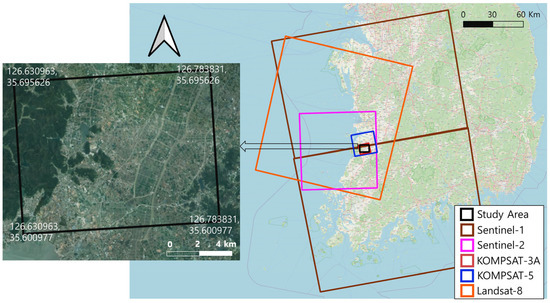
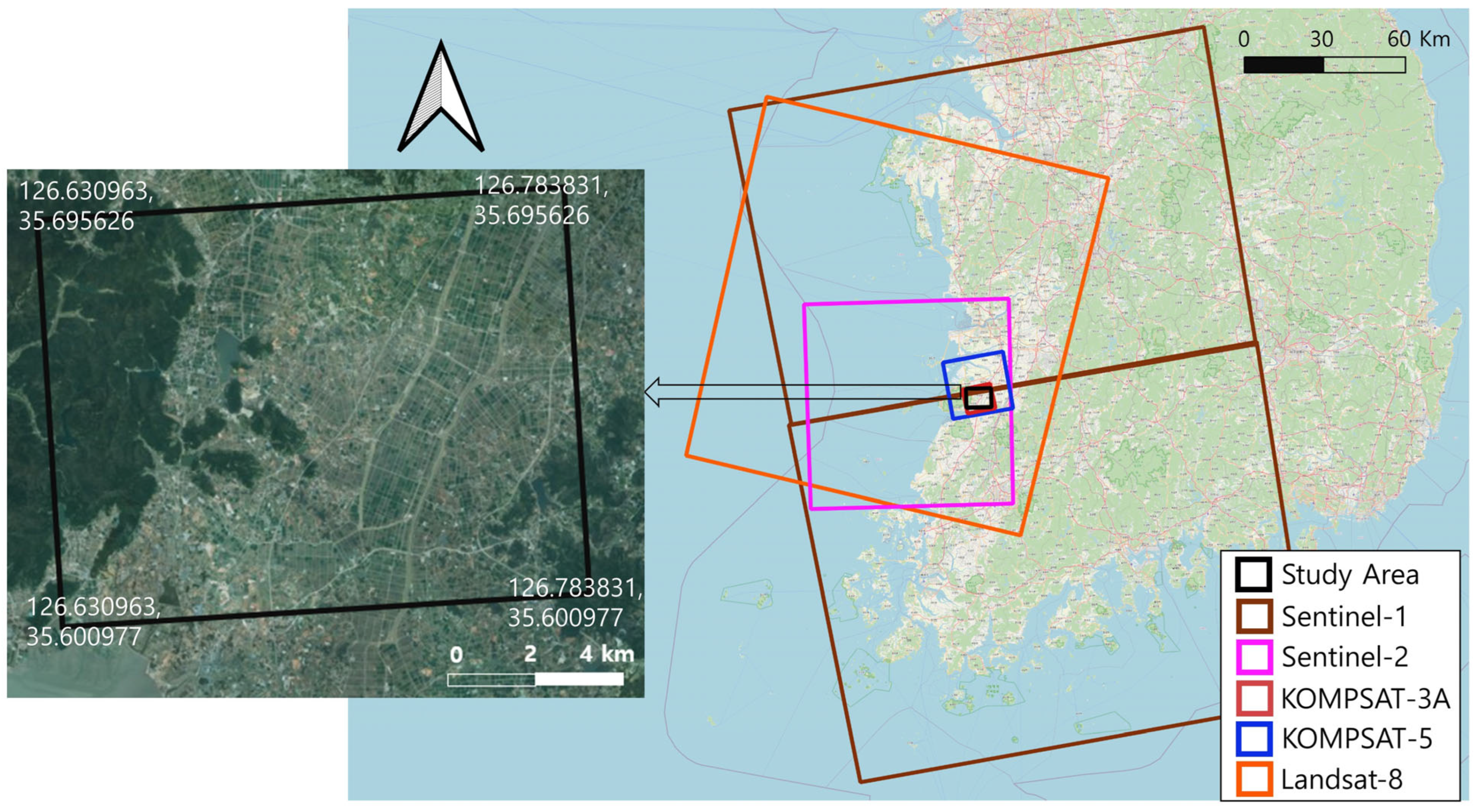
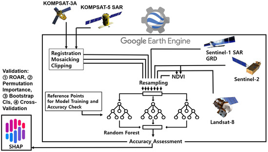
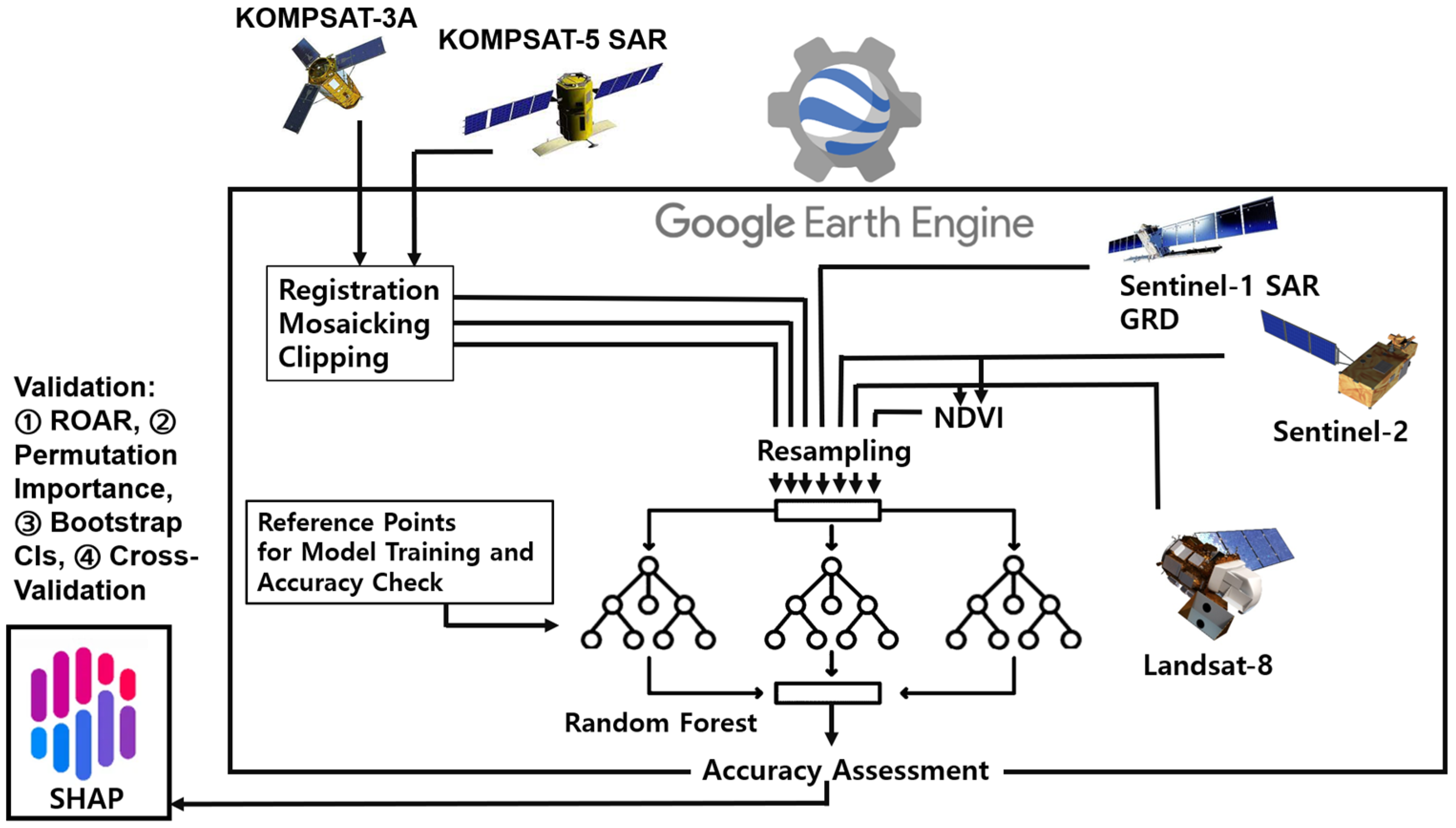
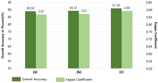
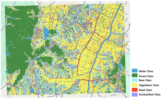
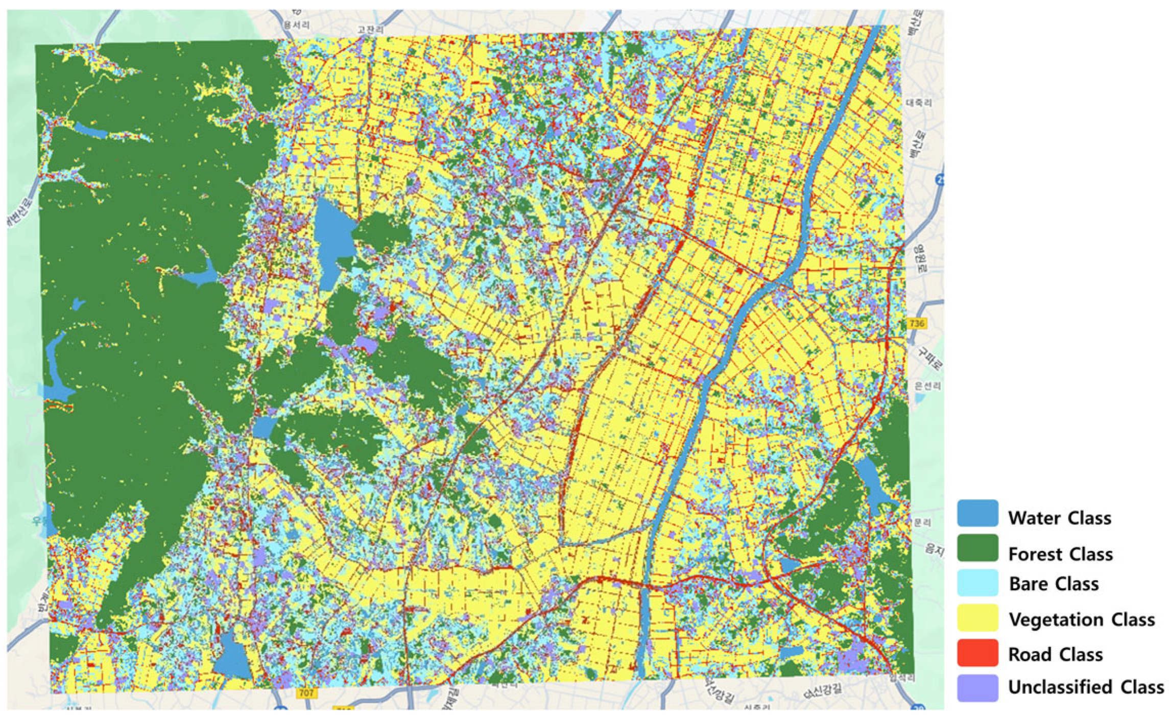
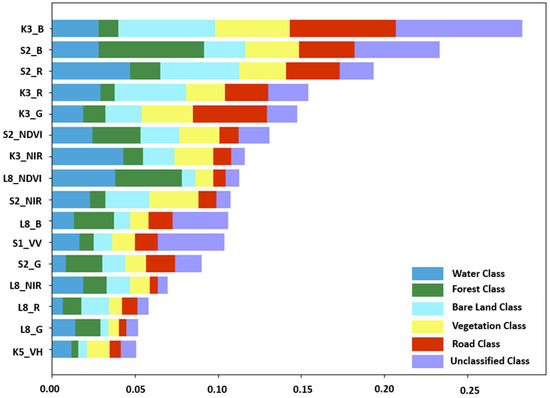
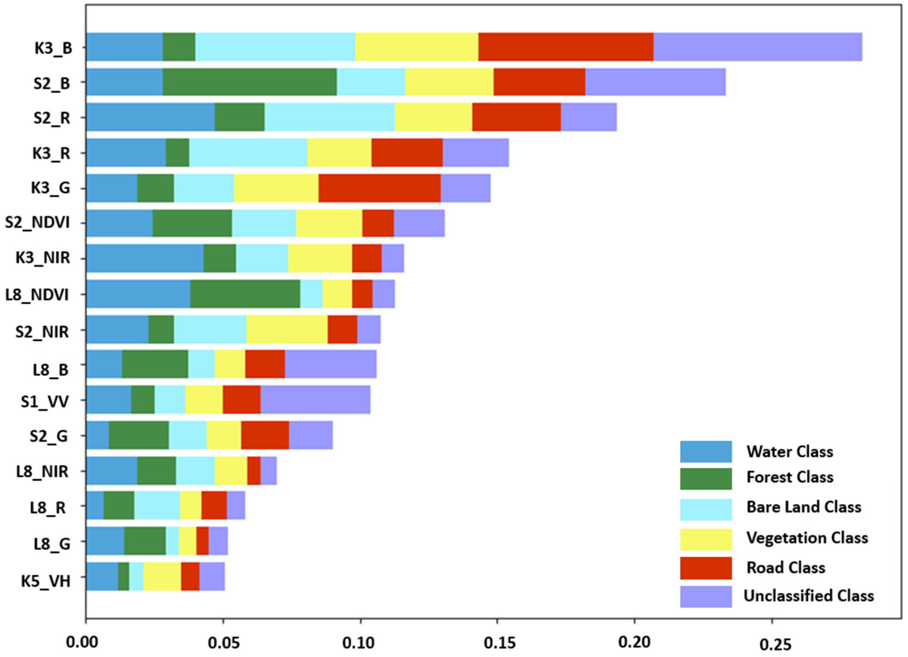
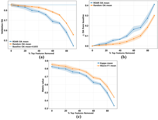
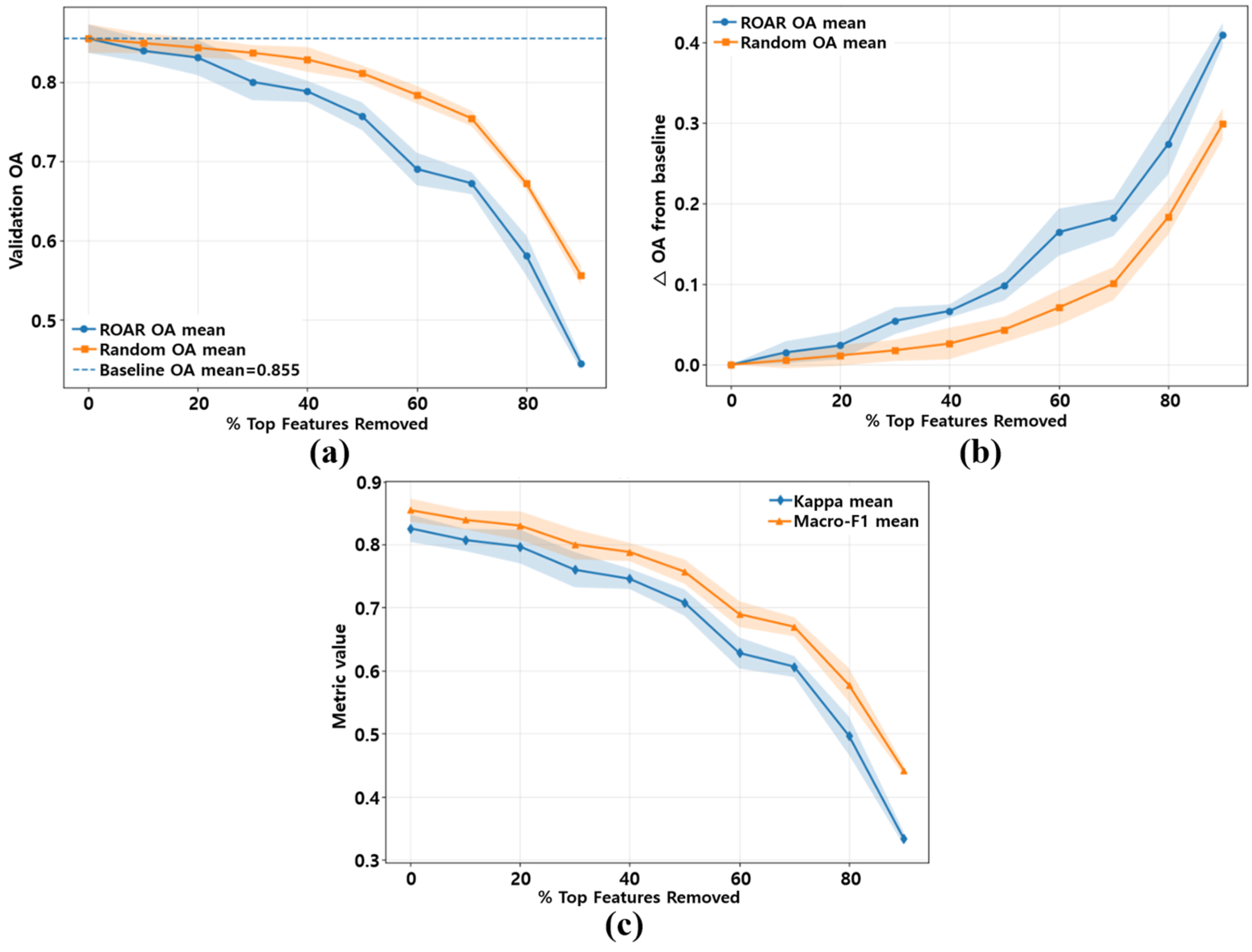
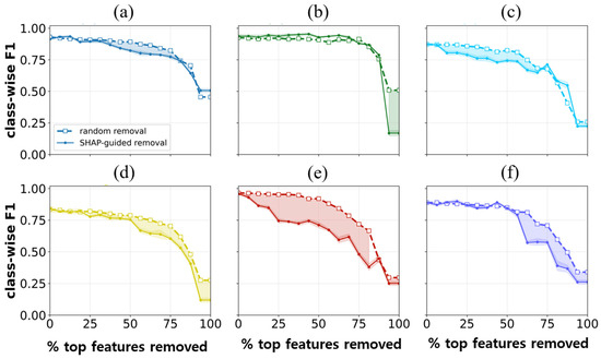
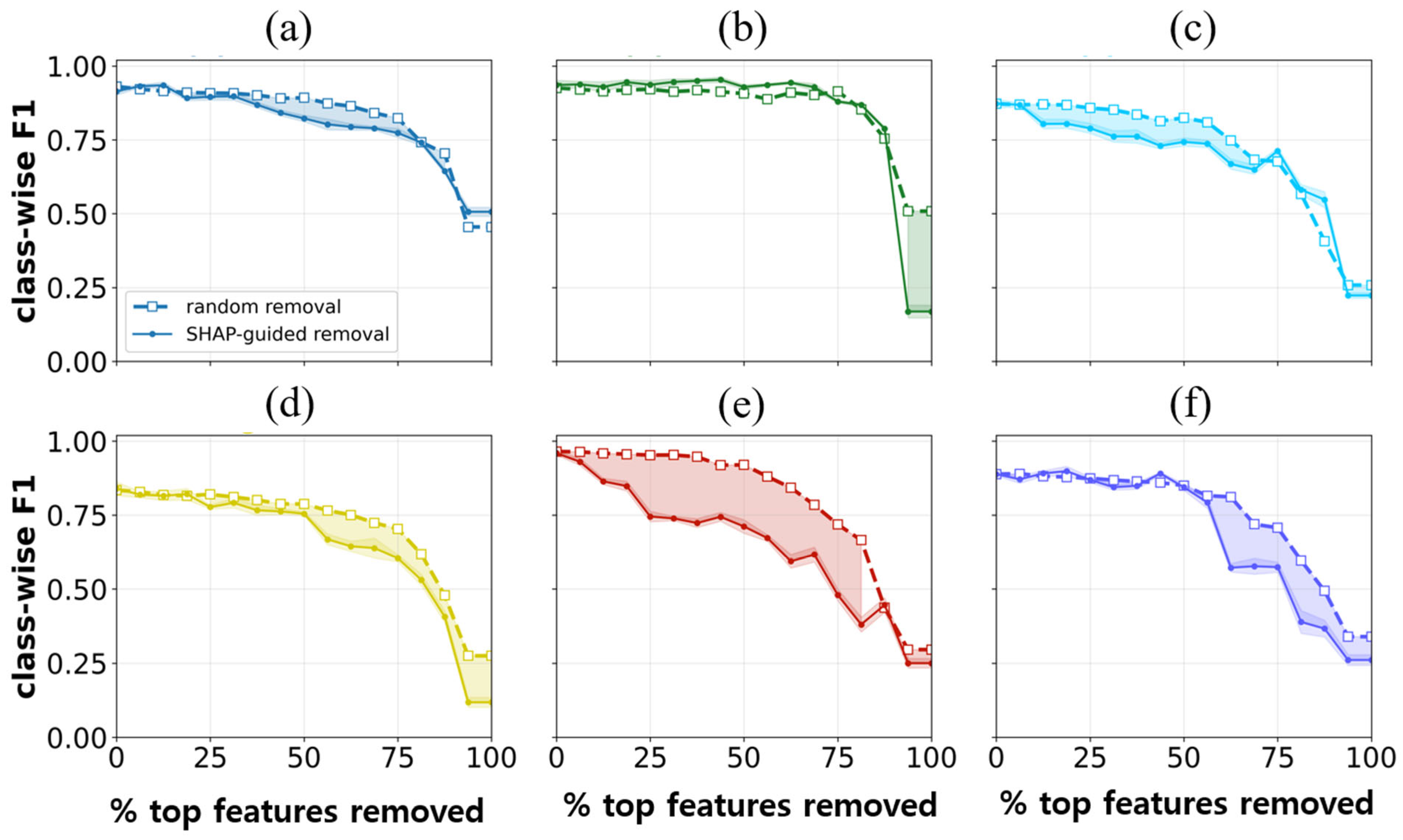
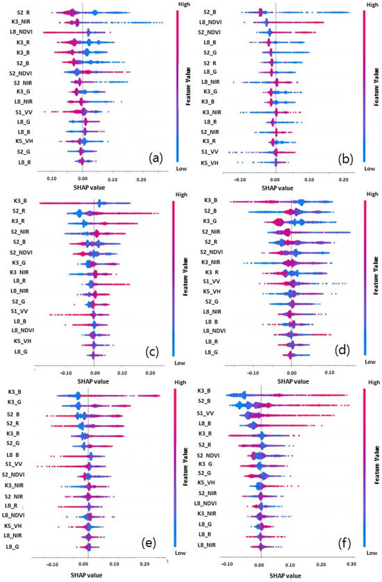
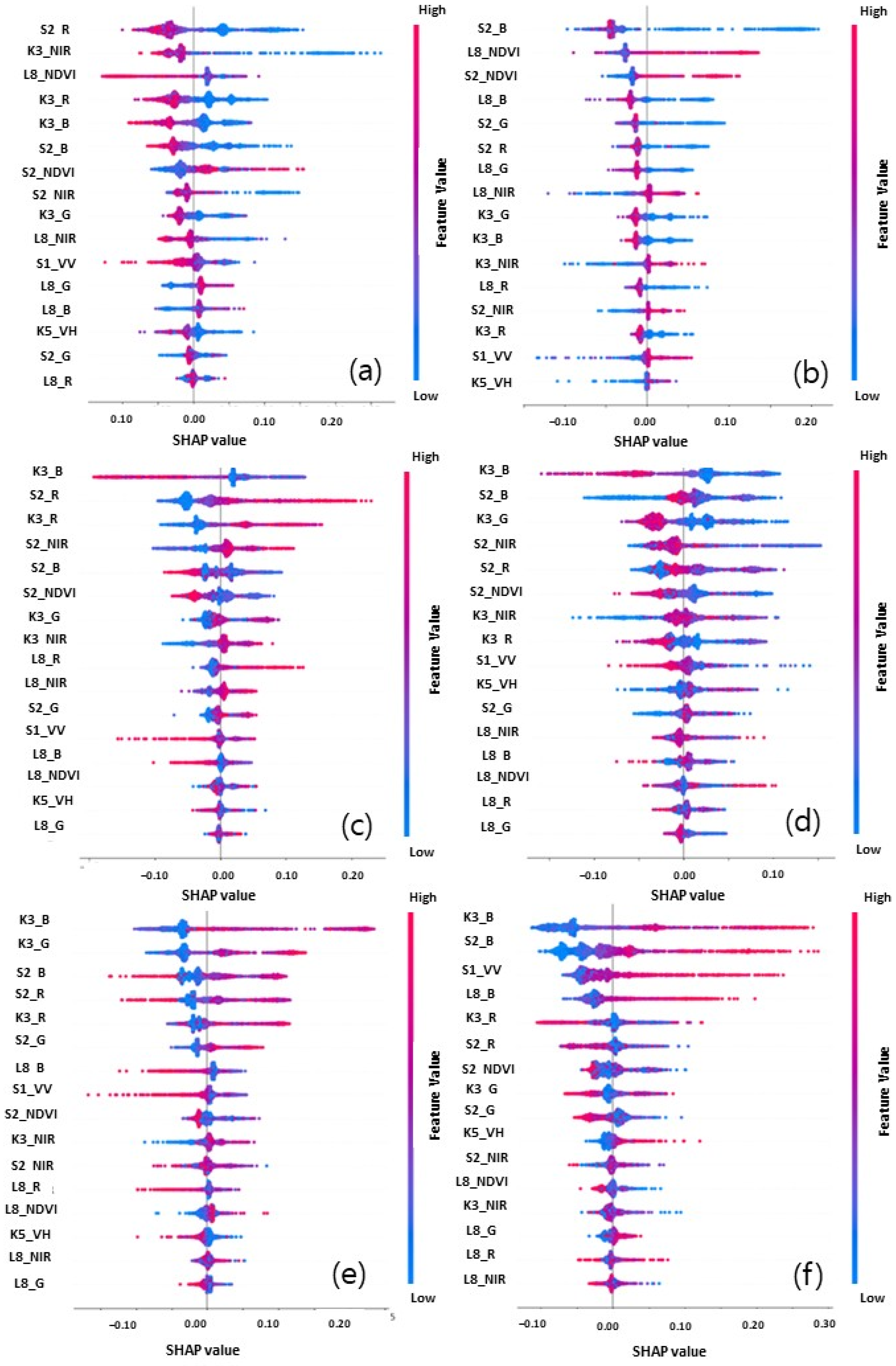
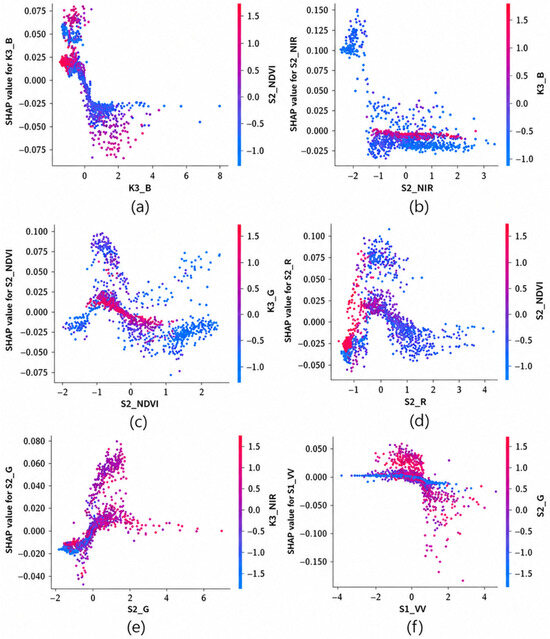
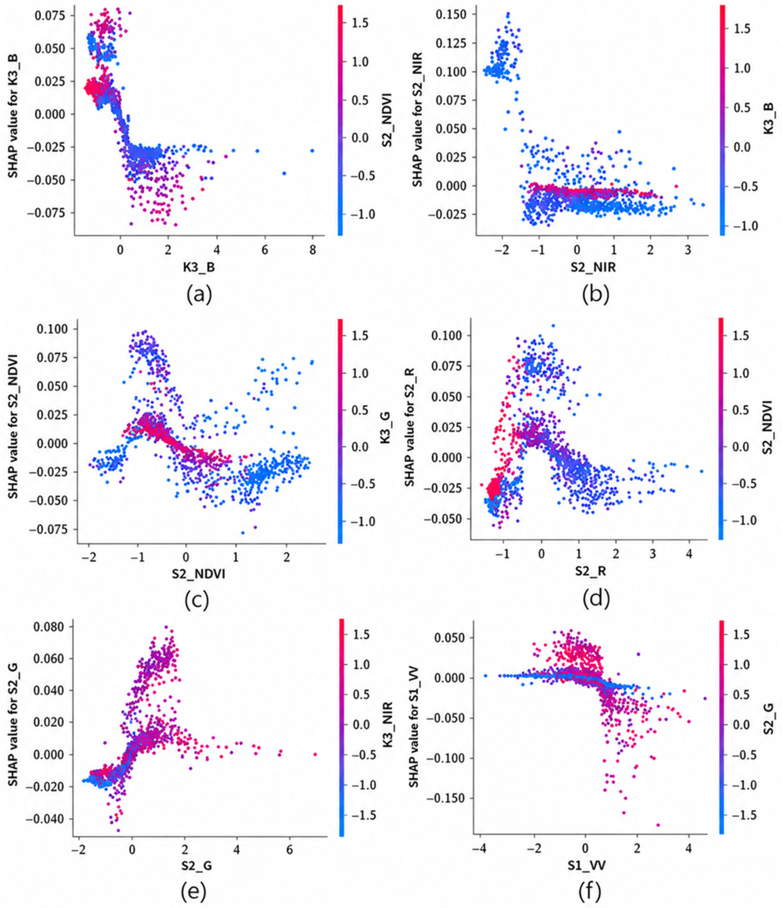
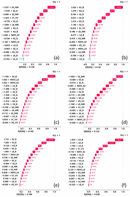
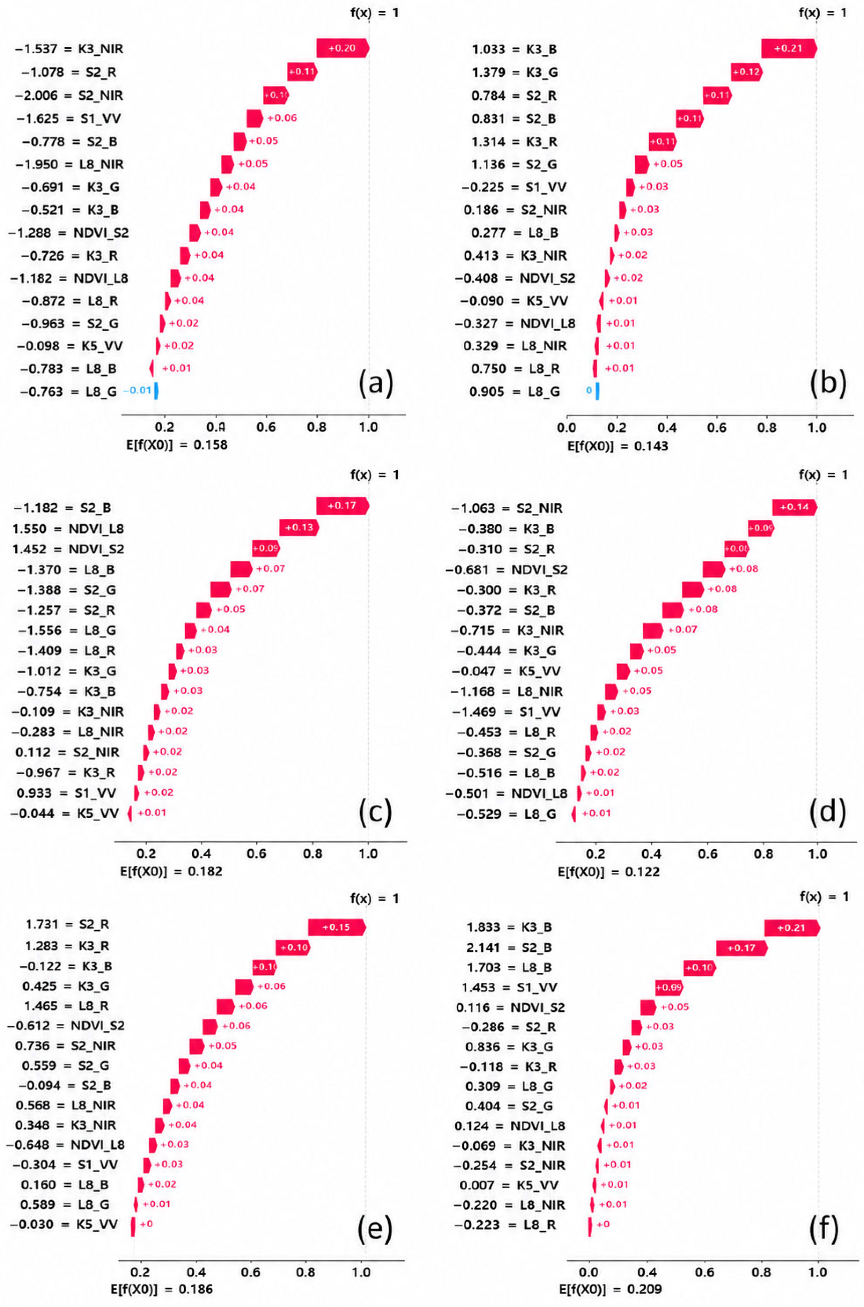
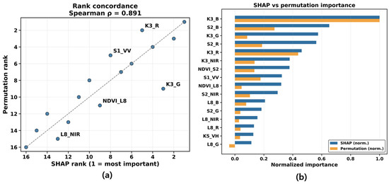
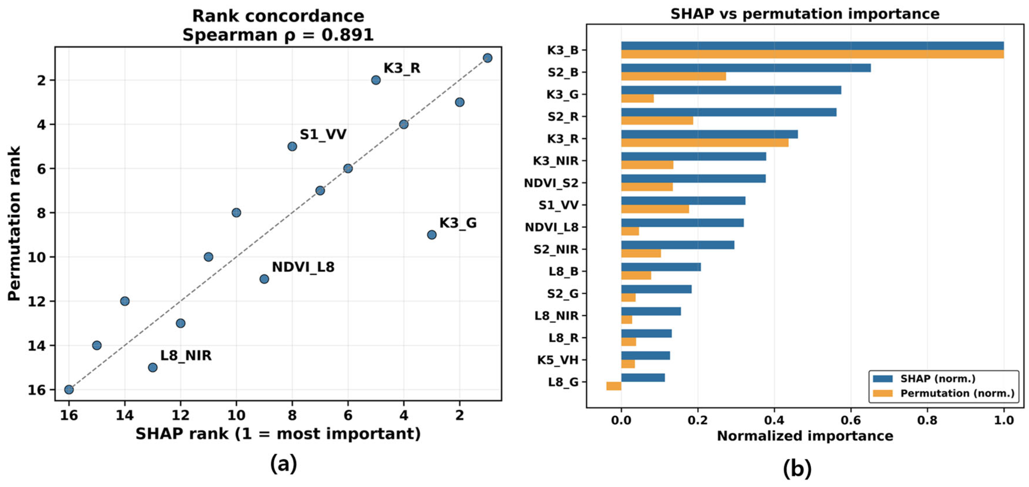
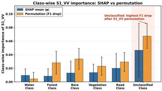
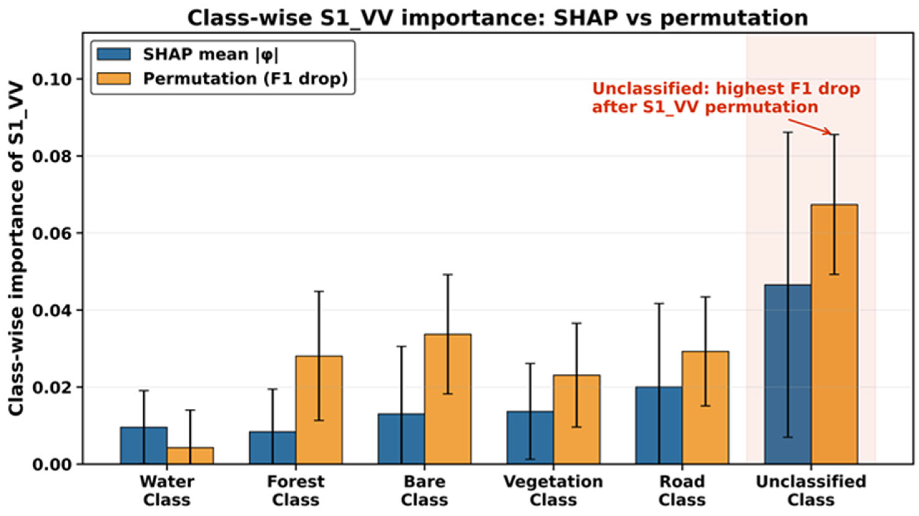
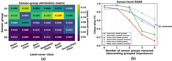
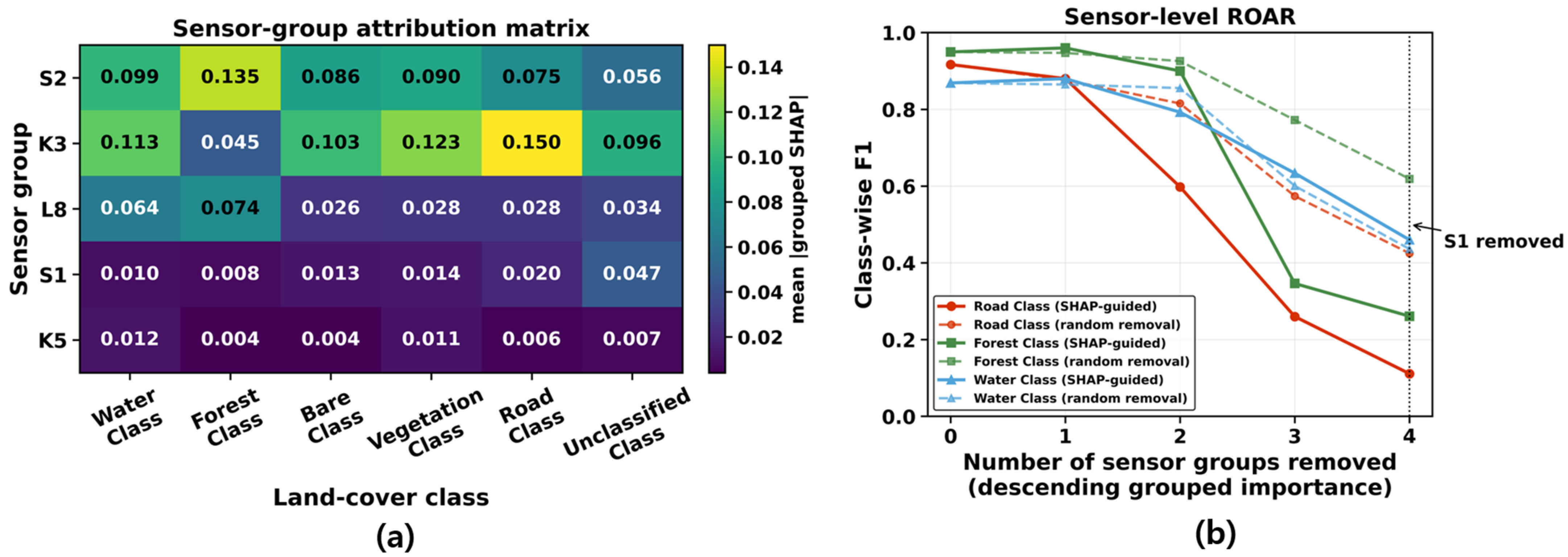
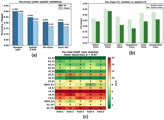
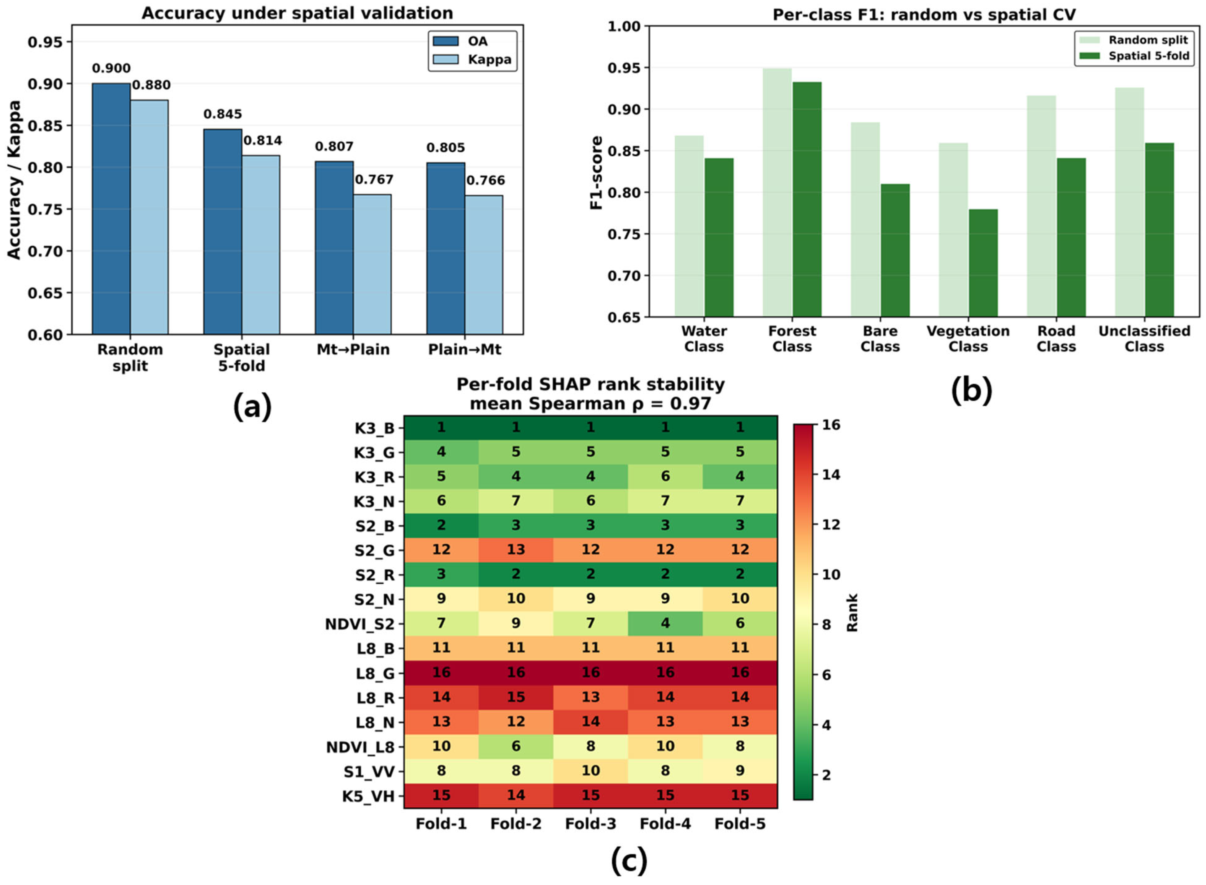
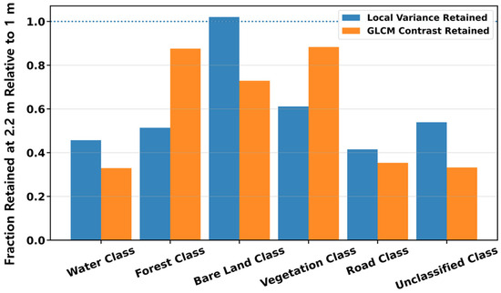
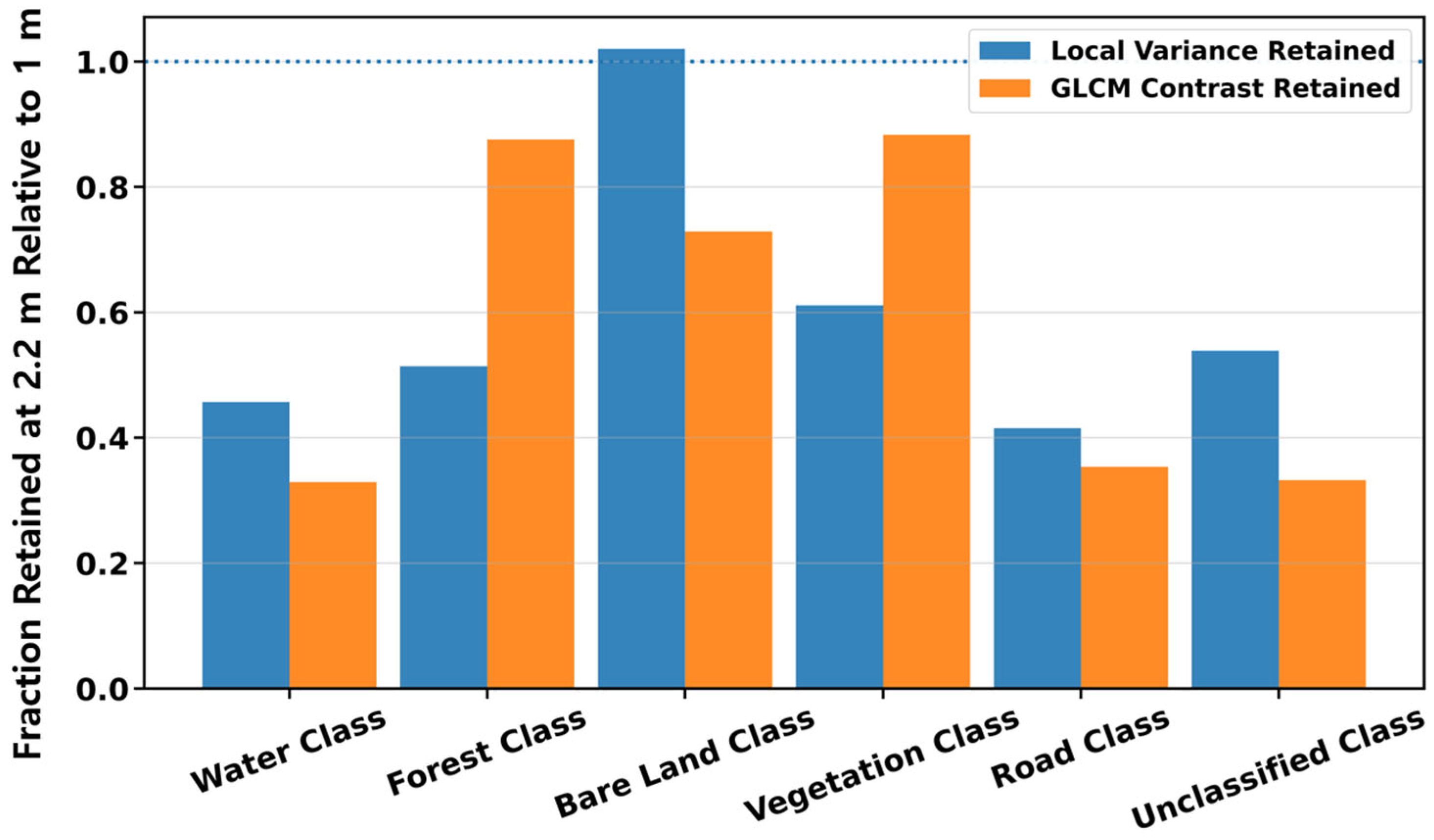
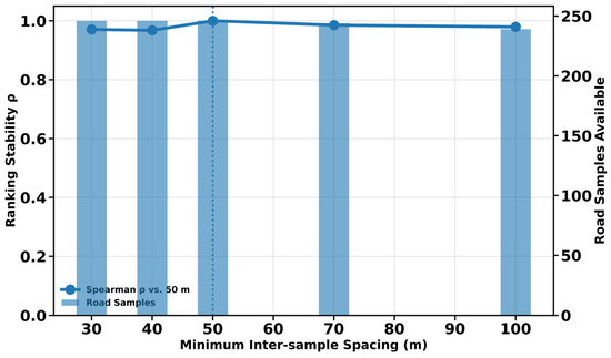
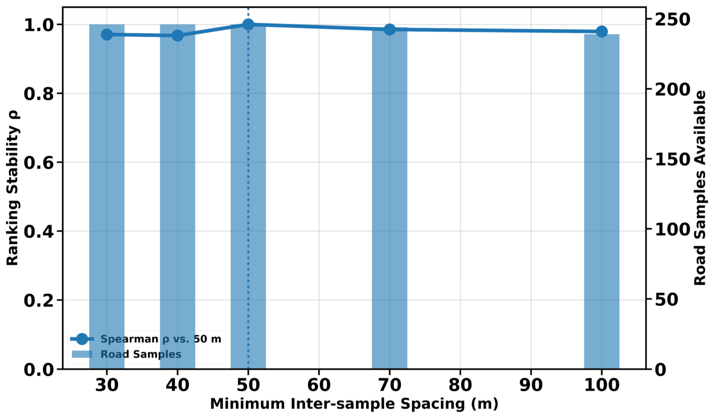

Disclaimer/Publisher’s Note: The statements, opinions and data contained in all publications are solely those of the individual author(s) and contributor(s) and not of MDPI and/or the editor(s). MDPI and/or the editor(s) disclaim responsibility for any injury to people or property resulting from any ideas, methods, instructions or products referred to in the content. |
© 2026 by the authors. Licensee MDPI, Basel, Switzerland. This article is an open access article distributed under the terms and conditions of the Creative Commons Attribution (CC BY) license.