


Abstract
Maintaining mechanical stability and achieving precise motion control on cylindrical surfaces remain critical challenges for underwater jacket cleaning robots. To address these issues, a systematic mechanical model is initially established for a standard column (diameter 2000 mm, inclination angle 90°) to determine stable climbing conditions. By neglecting equivalent gravity, the critical constraint relationships between adhesion and propulsion forces are derived. Subsequent open-loop maneuvering simulations, conducted via a six-degree-of-freedom dynamic model in MATLAB/Simulink, reveal that the robot achieves a straight-line speed of 0.233–1.601 BL/s and a maximum steady-state thrust of ~80 N at rotational speeds between 500 and 3000 rpm, and this thrust level corresponds to a required maximum adhesion force of approximately 106.4 N. To enable autonomous navigation, a closed-loop control system is developed for two-dimensional waypoint tracking, integrating line-of-sight (LOS) guidance, a waypoint switching radius strategy, and a proportional-derivative (PD) controller. Simulation results verify that the robot successfully navigates through five sequential turning waypoints under operational constraints, maintaining well-converged position and heading errors, with the maximum heading deviation controlled within ±5°. All simulation validations in this study are completed through numerical simulations in the MATLAB/Simulink environment. These findings offer a practical reference and theoretical foundation for the autonomous control and reliable deployment of underwater cleaning robots.
1. Introduction
With the rapid development of the global marine economy and the expansion of offshore wind and oil/gas industries, underwater jackets, as vital load-bearing units for offshore oil and gas platforms, offshore wind power foundations, and other large-scale marine engineering structures, operate long-term in complex environments characterized by high salinity, strong corrosion, and wave–current coupling. Recent studies indicate that marine biofouling significantly alters the surface morphology and hydrodynamic characteristics of underwater structures, increasing added mass and drag, and further affecting structural fatigue life, operation and maintenance costs, and long-term safety [1,2,3,4]. Concurrently, microbiologically influenced corrosion, coating degradation, and the coupled damage between the fouling layer and the metal substrate also accelerate the performance degradation of marine steel structures [5,6]. Therefore, carrying out periodic, highly efficient, and low-damage cleaning and maintenance for the attachments on jacket surfaces is an essential technical procedure to guarantee the safe operation of marine platforms and prolong structural lifespan.
Traditional jacket cleaning operations primarily rely on divers carrying high-pressure water guns or brushing tools for manual treatment; however, this operational method is significantly restricted by factors such as water depth, ocean currents, visibility, sea state windows, and human diving limits. It suffers from issues including low efficiency, high cost, substantial risks, and inconsistent cleaning quality. In recent years, water jet, cavitating jet, and robotic cleaning technologies aimed at ship hulls, jackets, and other underwater steel structures have received widespread attention. Related studies have systematically analyzed the influencing factors of high-pressure water jets in removing biofouling from the perspectives of cleaning mechanisms, nozzle parameters, pump pressure, standoff distance, moving speed, and surface damage control [7,8]. This provides an important reference for underwater cleaning robots to be equipped with efficient cleaning actuators and achieve engineering applications.
The development of underwater robotics technology offers a new automated approach for the inspection, cleaning, and maintenance of marine structures. Compared to manual diving, robotic systems possess advantages such as prolonged operational time, high repeatability, reduced personnel risk, and the ability to integrate sensory and inspection equipment. In recent years, domestic and international researchers have conducted extensive studies on ship hull cleaning robots, structural inspection robots, biomimetic underwater inspection robots, and adhesion-based underwater operational robots. This has led to the formation of various technical routes, including magnetic adhesion, negative pressure adhesion, thruster-pressed adhesion, crawler walking, wheeled crawling, and robotic arm cleaning [9,10]. Among them, wall-climbing cleaning robots designed for the cylindrical surfaces and variable-curvature steel pipes of jackets need to simultaneously address issues such as curvature adaptation, reliable adhesion, wave–current disturbance resistance, and the coupling of cleaning reaction forces.
Focusing on jacket cleaning scenarios, the stable operational capability of the robot on cylindrical column surfaces is the key factor determining system feasibility. Existing research indicates that marine organisms attached to the jacket surface, such as barnacles, shellfish, and algae, increase the structural load-bearing area and intensify wave and current loads, thereby affecting the robot’s adhesion safety margin and operational flexibility [11]. Consequently, the robot design must not only consider the static balance among its own gravity, buoyancy, propulsive force, adhesion force, and friction, but also incorporate external loads such as waves, currents, and the reaction forces of the cleaning actuator. This requires establishing an operational state analysis model applicable to typical jacket columns to provide a basis for matching adhesion forces, propulsive forces, and driving structure parameters [12].
In terms of dynamic modeling and simulation, underwater robots are jointly affected by added mass, nonlinear damping, restoring forces, thruster propulsive forces, and environmental disturbances, causing their motion to typically exhibit strong coupling, severe nonlinearity, and parametric uncertainty. Recent studies generally employ six-degree-of-freedom nonlinear models to describe the spatial motion of underwater robots, analyzing hydrodynamic parameters and motion responses in conjunction with system identification, CFD data, extended Kalman filters, long short-term memory networks, and simulation platforms like MATLAB/Simulink [13,14,15]. For jacket cleaning robots, establishing an open-loop maneuvering simulation platform helps predict straight-line speed, thrust output, and attitude response under different thruster rotational speeds, providing support for subsequent controller design and actuator selection.
Regarding motion control, underwater cleaning robots must achieve stable path following under conditions of current disturbances, model uncertainties, actuator saturation, and nonlinear thrust mapping. In recent years, methods such as line-of-sight (LOS) guidance, improved LOS guidance, model predictive control, sliding mode control, robust adaptive control, fuzzy sliding mode control, and reinforcement learning-assisted PID have been widely applied to AUV path tracking and waypoint following problems [16,17,18,19,20]. Among these, LOS guidance is highly suitable for converting target waypoint positions into desired headings due to its concise form and convenience in engineering implementation; meanwhile, PD/PID control remains appropriate as a foundational control law during the engineering prototype and simulation verification stages because of its clear structure, intuitive parameter tuning, and low computational load.
In summary, research on the operational state analysis and motion control of underwater jacket cleaning robots involves multi-disciplinary domains, including marine biofouling, robotic adhesion and locomotion mechanisms, hydrodynamic modeling, guidance and control, and simulation verification. Existing research has laid the foundation for underwater cleaning robots from structural design to autonomous control. However, three specific gaps remain: the lack of systematic analysis of the propulsion–adhesion constraint for large-diameter jacket columns, the absence of an integrated six-DOF dynamic simulation framework, and the insufficient validation of waypoint tracking control strategies for jacket structures. Based on this, targeting typical operational conditions of underwater jacket cleaning robots on column surfaces, this paper establishes a mechanical model of the operational state and an open-loop maneuvering simulation platform. To address these gaps, it further designs a closed-loop motion control system integrating LOS guidance, a waypoint switching radius strategy, and a PD control law to verify the robot’s stable operational and waypoint-following capabilities. The simulation results demonstrate that the robot achieves stable climbing constraints, reaching straight-line speeds of 0.233–1.601 BL/s within designated thruster limits. Moreover, the proposed control system enables the robot to sequentially navigate turning waypoints with well-converged position and heading errors, providing a reliable technical reference for autonomous jacket cleaning operations.
However, the primary objective of this paper is to demonstrate the theoretical feasibility and basic performance of the proposed control scheme under nominal conditions. Rather than attempting to incorporate all practical disturbances and uncertainties—such as sensor noise, time delays, actuator rotational speed saturations, ocean-current disturbances, and parameter variations—we focus on establishing the fundamental validity of the control architecture in a clean, well-defined setting. This preliminary numerical feasibility analysis serves as a first step toward more realistic implementations, and the results obtained herein provide a solid baseline for future robustness enhancements.
2. Operational State Analysis of the Jacket Cleaning Robot
Under the operational state on the surface of the jacket column, the cleaning robot is subjected to six external forces: gravity of its own weight and payload , thruster forward propulsive force , the robot’s adhesion force , normal support force from the column surface , friction force , and water buoyancy . The resultant force of the robot’s gravity and the buoyancy it experiences in water can be denoted as the robot’s equivalent gravity . On the one hand, the friction force generated by the adhesion force serves as an effective driving force for the robot to resist the gravity component and prevent sliding; on the other hand, during the robot’s motion, the friction force also acts as a crawling resistance. When the robot is stationary, two primary failure modes may occur during operation: falling off and overturning. To meet the underwater operational conditions and achieve stable crawling on typical jacket columns, a column with a diameter of 2000 mm (maximum specification) and a horizontal inclination angle of 90° is selected as the analysis object to conduct an overall mechanical analysis of the robot.
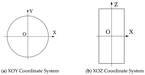
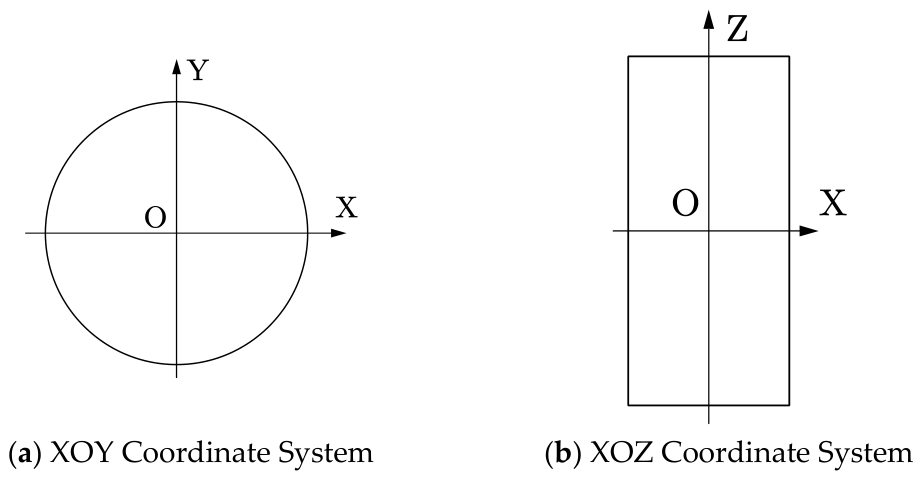
A three-dimensional coordinate system is established with the base of the jacket column as the origin. The coordinate system is constructed with the circular cross-section of the column as the XOY plane and the upright section of the column as the XOZ plane, as shown in the corresponding Figure 1.
Figure 1.
Jacket Column Coordinate System.
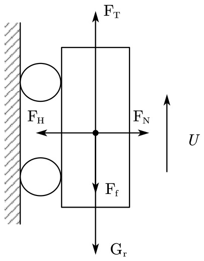
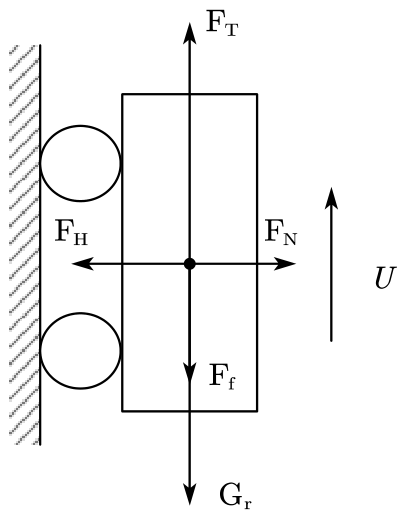
To prevent the robot from falling off the jacket while operating on the column, the XOZ plane of the robot on the jacket needs to be taken as the research object. In this case, to maintain stability, the sum of the friction force between the robot and the jacket column and the robot’s own equivalent gravity must be less than or equal to the forward propulsive force of the thruster. As illustrated in the corresponding force state diagram (Figure 2). This yields:
Figure 2.
Diagram of the robot’s force state in the XOZ coordinate system.
Furthermore, according to Newton’s third law, the robot’s adhesion force and the support force exerted by the jacket column on the robot are equal in magnitude and opposite in direction, i.e., . Assuming the friction coefficient between the jacket column (steel) and the rollers (rubber) is , and taking a safety factor of 1.5, the mechanical condition at this point becomes:
By consulting mechanical design manuals, the friction coefficient between the jacket column (steel) and the rollers (rubber) is 0.5. The robot has a mass of 150 kg, giving a self-weight of = 1471.5 N. Its displaced volume is approximately 0.150 m3, and the buoyancy force provided by seawater is = 1471.2 N. Thus, the equivalent gravity is ≈ 0.3 N. This value accounts for only 0.4% of the maximum steady-state thruster thrust (~80 N), indicating that the installed buoyancy material can provide buoyancy nearly equal to the robot’s self-weight. Therefore, the equivalent gravity of the robot can be neglected. Finally, it can be concluded that the robot’s adhesion force must satisfy the following constraint: . For the specific dimensions of the robot and the position parameters of the actuators, please refer to Appendix A.
3. Construction of an Open-Loop Simulation Analysis Platform for the Robot’s Operational State Based on the Theoretical Model
3.1. Theoretical Model
An open-loop maneuvering model of the underwater cleaning robot is constructed between the Earth-fixed coordinate system and the body-fixed coordinate system attached to the robot, which is described by the following Equations (3) and (4). The input of the model is the control command u of the actuators, and the output is the position and attitude of the underwater cleaning robot in the Earth-fixed coordinate system.
Here, represents the generalized velocity vector; represents the generalized velocity vector considering ocean current disturbances, where the disturbance forces of the current are represented by the relative velocity (i.e., the velocity of the robot relative to the current); denotes the position and attitude vector; denotes the coordinate transformation matrix; is the generalized mass matrix; is the generalized centripetal and Coriolis matrix; is the damping force matrix; represents the restoring force vector; and represents the propulsion force provided by the actuators. Furthermore, , where represents the rotational speed of the thrusters. The specific parameters and solution method of the coefficient matrix mentioned in Equation (2) are provided in the Appendix B. For the actuator model, please refer to Appendix C. To simplify the analysis process, during the operation of the robot, the adhesion forces provided by the vertical thrusters and the magnetic adhesion driving wheels are determined by the formula .
3.2. Construction of the Open-Loop Simulation Analysis Platform
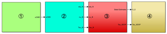
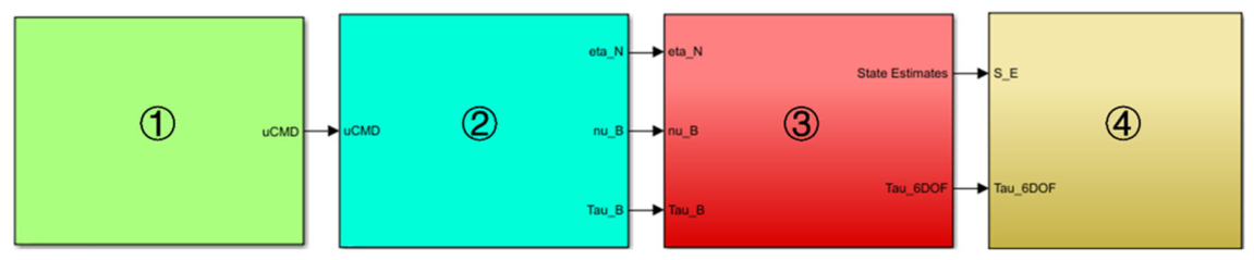
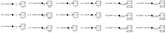
Based on the previously designed and derived mathematical and dynamic models of the underwater cleaning robot’s motion, an open-loop maneuvering simulation platform was built in the MATLAB/Simulink R2023b environment, and its structure is shown in Figure 3. The simulation model consists of four encapsulated modules: (1) Control parameter input; (2) System model (kinematics and dynamics); (3) Attitude and position conversion module (converting the attitude description from quaternions to Euler angles); (4) Motion state and control force observation module.
Figure 3.
Simulink open-loop maneuvering simulation model of the system.
During the three-dimensional spatial motion of the robot underwater, the rotational speeds , , and of the two horizontal propeller thrusters (HP1 and HP2) and the two vertical propeller thrusters (VP1 and VP2) are used as the control input signals of the control system. When the rotational speeds and of HP1 and HP2 are equal, the robot moves in a straight line in the XOY plane; when and are unequal, the robot performs a yawing motion. The rotational speeds of VP1 and VP2 are always kept equal to to control the heaving motion of the robot.
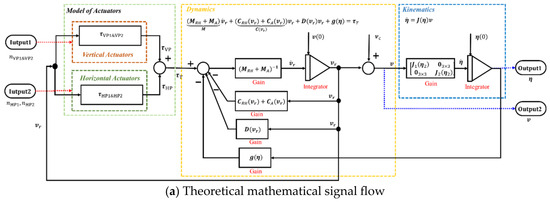
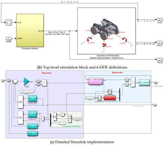
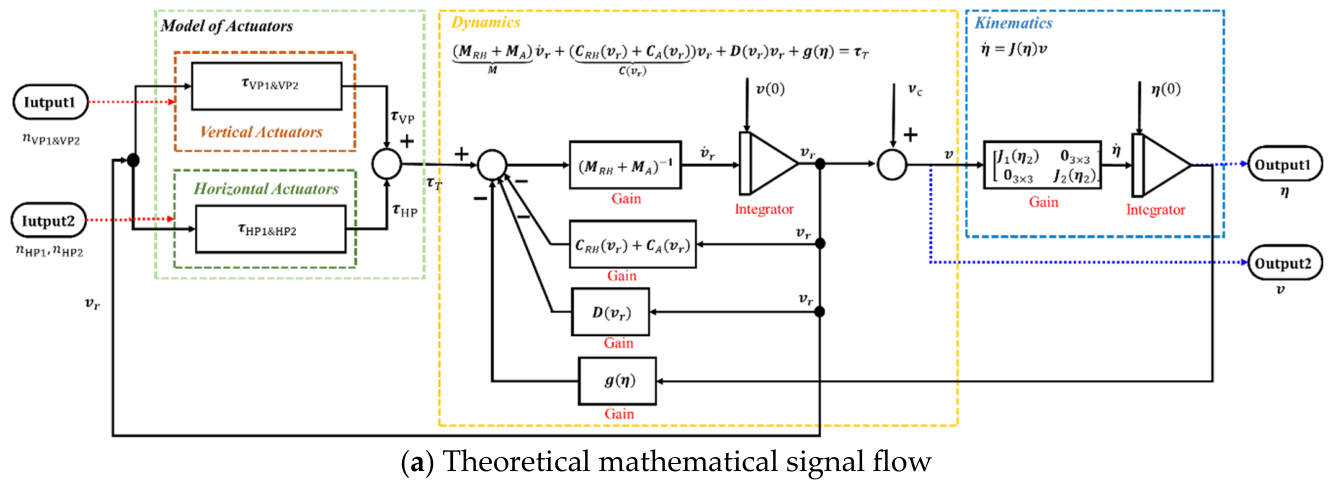
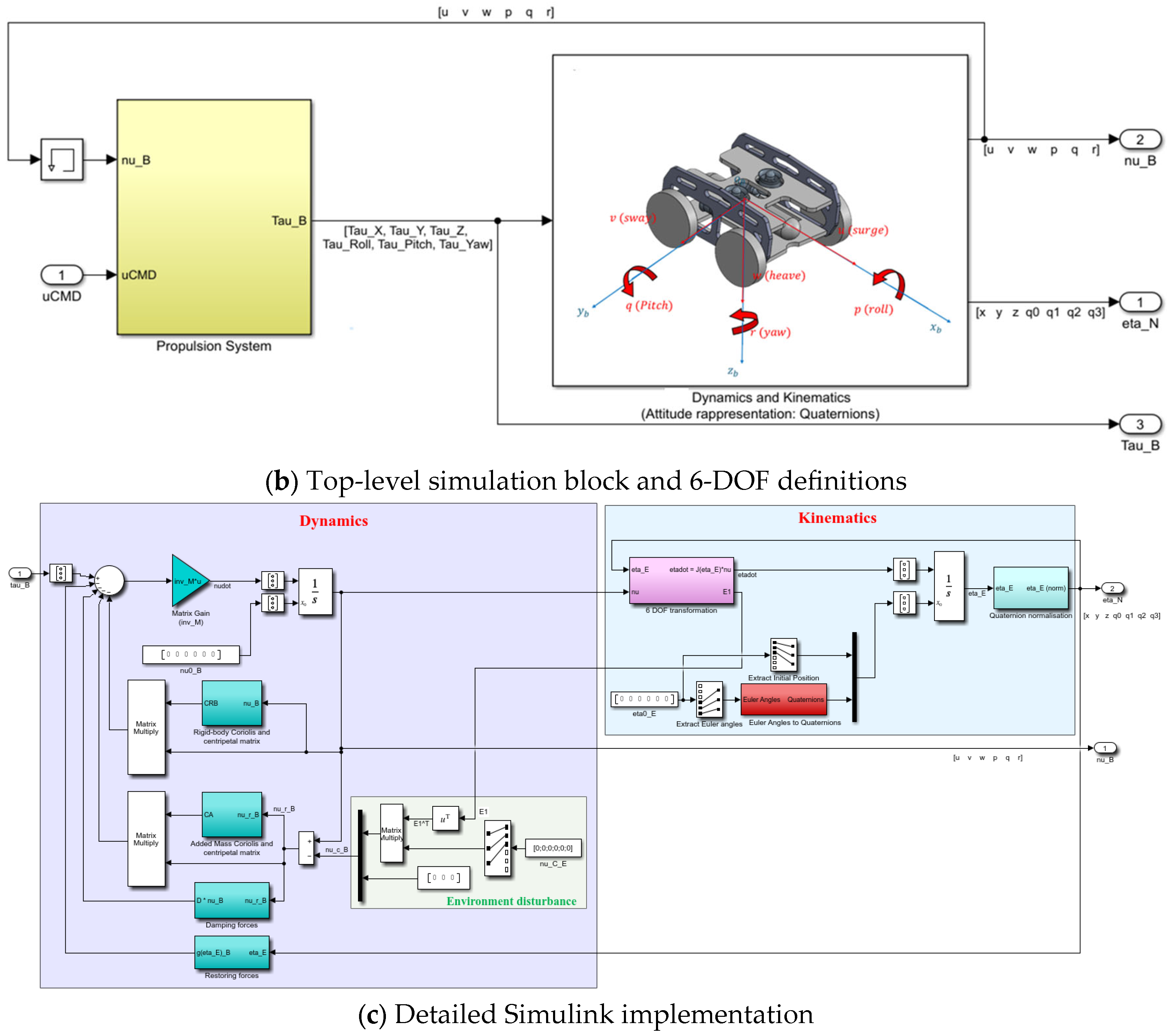
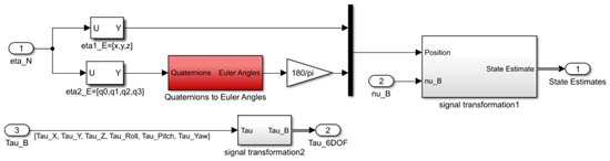
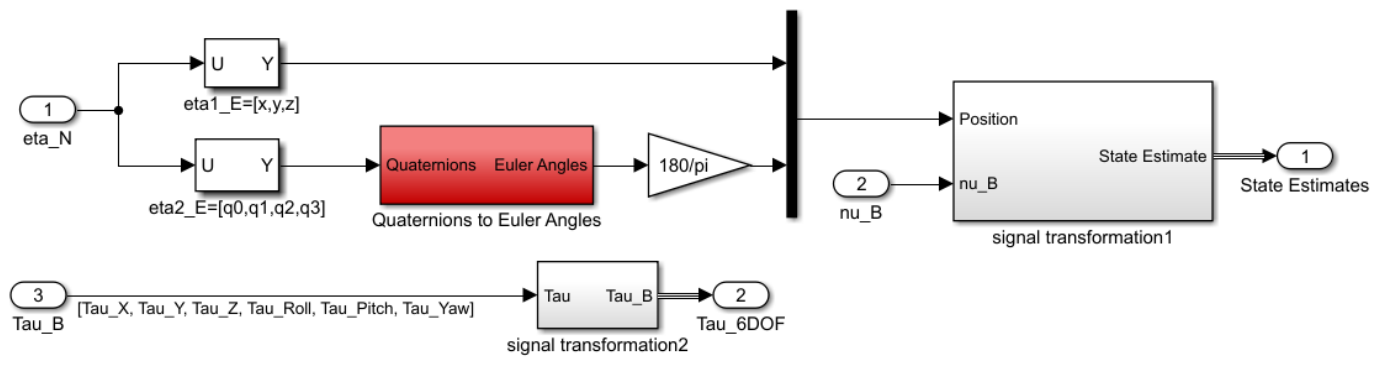
Figure 4 shows the detailed structure of the system model module. The overall block diagram is presented in Figure 4a. The internal structure is shown in Figure 4b, where the yellow-highlighted subsystem on the left represents the robot’s propulsion system. Under given control parameter inputs, the total driving control force generated by the robot’s motion actuators can be calculated using the thruster driving force formula. In the right subsystem, the kinematic and dynamic equations that constitute the mathematical model of the robot are implemented. All the driving forces and kinematic/dynamic equations discussed are represented by the block diagram shown in Figure 4a. Figure 4c illustrates the internal structure of the mathematical model subsystem of the underwater cleaning robot, taking into account environmental disturbances from ocean current velocities. Within this subsystem, the vector representing the attitude is described using the Euler angle method for internal transmission, and it is converted into unit quaternions when outputting from the subsystem. In addition, Figure 5 and Figure 6 display the internal structures of the attitude and position representation conversion module and the motion state and control force observation module, respectively. This completes the construction of the open-loop maneuvering simulation model platform.
Figure 4.
System model module. (a) theoretical mathematical signal flow; (b) top-level simulation block and 6-DOF definitions, where u, v, and w denote translational velocities, and p, q, and r denote angular velocities; (c) detailed Simulink implementation. The asterisk denotes matrix–vector multiplication in MATLAB/Simulink notation.
Figure 5.
Attitude and position representation conversion module.
Figure 6.
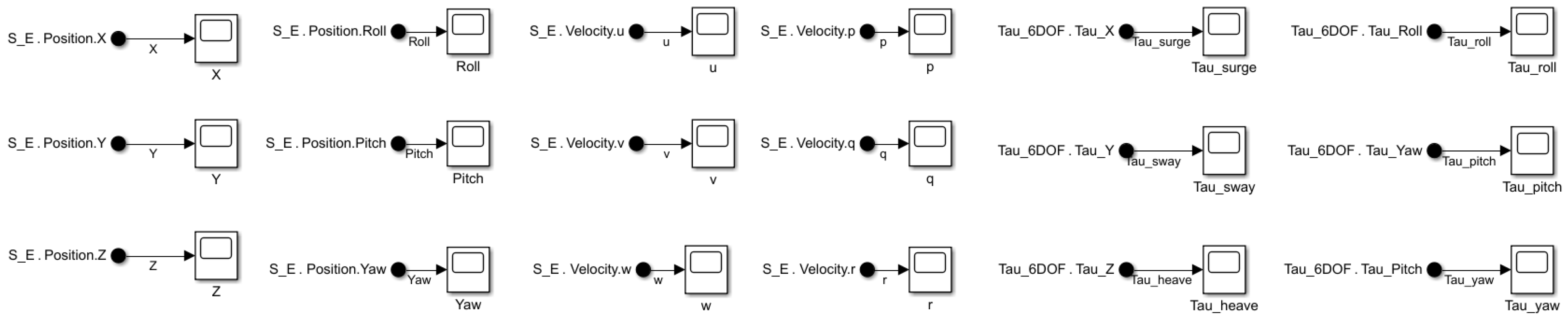
Motion-state and control-force observation module, where x, y, and z denote positions; u, v, and w denote translational velocities; p, q, and r denote angular velocities; and the corresponding τ terms denote the generalized control forces and moments.
3.3. Open-Loop Maneuvering Simulation Results
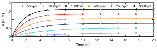
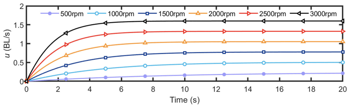
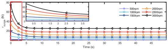
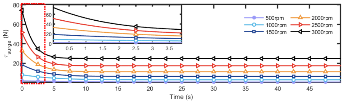
Prior to designing the closed-loop control system for planar motion, the motion performance of the robot was tested by applying given control inputs. The straight-line speed of the robot directly demonstrates its locomotive capability. In the Simulink platform, the straight-line speed of the robot in the horizontal plane was analyzed under the condition that the horizontal propeller thrusters provide forward thrust. Different cruising speeds can be obtained by varying the thruster rotational speed. Figure 7 and Figure 8 show the planar motion velocity and thruster forward thrust curves at different propeller thruster rotational speeds, respectively. Results show that, as the thruster rotational speed increases, the robot’s steady forward speed increases gradually, and the time to reach steady state is shortened. Within the rotational speed range of 500–3000 rpm, the robot’s straight-line speed can reach 0.233–1.601 BL/s (robot body length m), and the maximum steady-state thrust provided by the thrusters can reach approximately 80 N. Therefore, the maximum required adhesion force is around 106.4 N.
Figure 7.
Time–history curves of the robot’s straight-line speed under propeller thruster mode.
Figure 8.
Time–history curves of the robot’s forward thrust under propeller thruster mode.
4. Control Performance Analysis
4.1. Guidance and Waypoint Switching Strategy
In the path-following problem of underactuated underwater vehicles, the guidance law plays an important role. Line-of-sight (LOS) guidance strategy has become the most widely adopted mainstream solution in this field due to its concise implementation framework and reliable path-following capability [21].
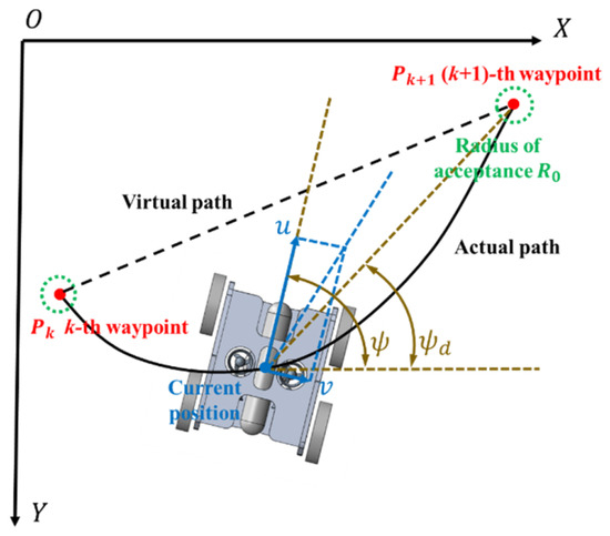
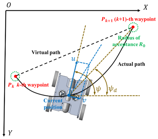
During operation, the robot adheres to the jacket surface, and its motion can be approximated as two-dimensional planar motion. Let the target waypoint position in the 2D plane be denoted as . A 2D LOS guidance law is adopted, with the objective of reaching the and coordinates of the waypoint. To achieve the designated task, the guidance law calculates the distance deviation D between the waypoint position and the robot’s position at time t, as well as the heading reference command in real time:
The geometric relationship of the above LOS variables is illustrated in Figure 9. Therefore, the surge and heading motion errors of the underwater robot can be expressed as , where , and maps any angle into the interval , ensuring that the error remains bounded and continuous across the ±π boundary. This error vector is fed into the controller. Furthermore, the required position control path for the robot is described by N discrete waypoints given in the coordinate system, with adjacent waypoints connected by straight line segments. To ensure the continuity and smoothness of the robot’s movement along the predefined waypoint path, an “acceptance radius ” is introduced in the waypoint switching logic [22]. Specifically, when the robot enters a circular neighborhood of radius around the current waypoint , the target is updated to , and the robot continues along the path. This process iterates in a loop until the robot reaches the neighborhood of the final target waypoint , at which point the motion terminates.
Figure 9.
2D Line-of-Sight Guidance Method.
4.2. Control Strategy
4.2.1. Nonlinear Mapping Process
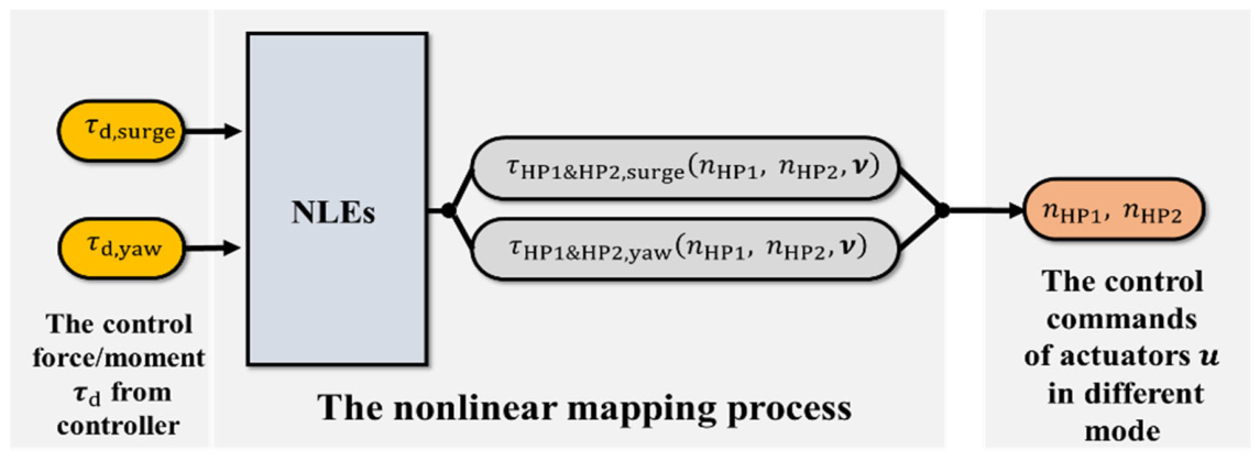
In the closed-loop motion control system of the underwater cleaning robot in this study, the output forces and moments from the controller undergo a process similar to “thrust allocation” to convert the control signals input to the robot from control forces into control commands for each actuator. This process is referred to as the nonlinear mapping from control forces to actuator commands. It aims to construct the inverse process of the actuator model , i.e., . For planar operation, we only control two degrees of freedom: surge and yaw. Therefore, represents the 2D control force/moment output by the controller.
Robots with nonlinear actuators must undergo this mapping step when implementing closed-loop motion control. The nonlinear thrust allocation process in this paper is essentially a numerical approach that takes the reference forces/moments output by the controller as known inputs and online solves the coupled nonlinear equations in the surge and yaw degrees of freedom, thereby obtaining the required rotational speed control variables for each thruster. This process transforms the high-level control commands into physical drive signals that the actuators can respond to, serving as the critical link between control decision-making and low-level propulsion execution. As shown in Figure 10, since we have already constructed the analytical model of the thrusters in previous studies, can be obtained by solving nonlinear equations (NLEs) online. Due to coupling between the surge and yaw control forces and moments, the Levenberg–Marquardt method is used to solve for the horizontal thruster commands, implemented via the fsolve function in MATLAB. In addition, the following techniques are applied for setting initial values during the numerical solving process:
- (1)
- Determine the signs of the actuator control commands and based on the sign of the control force/moment output by the controller.
- (2)
- The initial magnitude values of the actuator control commands and are set to the extreme values of their saturation constraints.
- (3)
- To achieve high-maneuverability in situ turning, the initial values of the control commands and for the HP1 and HP2 actuators are specifically designed: for straight-line motion, ; for turning, . The decision to execute straight-line motion or in situ turning depends on whether the heading angle error falls within the allowable tolerance , where in this paper.
Figure 10.
Schematic of the nonlinear mapping from controller forces and moments to horizontal-thruster commands.
Due to the complexity, strong nonlinearity, and time-varying characteristics of the mathematical model of the robot system, the control strategy for the closed-loop motion control system primarily selects a model-free control method that is concise in form and easy to design [23]. In this study, the PD control law is adopted for heading and position tracking. From an engineering perspective, the PD controller features a simple structure, physically meaningful parameters, and low computational cost. Moreover, compared with the standard PID controller, the pure PD controller eliminates the integral term, thereby effectively preventing integral windup and the associated heading overshoot. More importantly, the core contribution of this work lies in the feasibility validation of the guidance law and thrust allocation strategy, rather than a comparative study of high-order control algorithms. Given its maturity and proven reliability in industrial applications, the PD controller provides sufficient control performance for the intended guidance verification objectives.
Therefore, the control strategy ultimately adopts a hybrid architecture consisting of “PD outer-loop control + model-based thrust allocation”: the outer-loop PD controller is model-free and is responsible for generating the desired control forces based on the tracking errors; the inner-loop thrust allocation module, built upon the analytical actuator model, employs numerical methods to solve the nonlinear equations online to obtain the rotational speed commands for the thrusters.
4.2.2. PD Control Law
The PD controller model in the 2D state space of the controlled degrees of freedom is expressed as follows:
where and are gain vectors corresponding to the distance error and heading error, respectively; represent the system error and the rate of change of the system error, respectively. In addition, , . Since PD control is a single-input single-output (SISO) controller, for the 2D waypoint tracking task, it is necessary to design controllers separately for each controlled degree of freedom. The parameter tuning of the PD controller adopted in this study is carried out in two steps. First, initial gain values are obtained using the Ziegler–Nichols critical sensitivity method [24] on a simplified linearized model of the system. Second, these preliminary gains are manually fine-tuned in a fully nonlinear simulation model that incorporates hydrodynamic damping, nonlinear thrust mapping, and waypoint-switching logic, with response speed and overshoot as the trade-off criteria. Following the above tuning procedure, the final gain values are determined as: position loop , ; heading loop , .
4.3. Construction of the Closed-Loop Simulation Analysis Platform
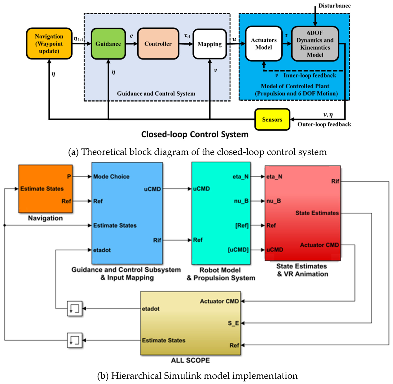
Combining the open-loop maneuvering model constructed in Section 3.2 with the waypoint switching strategy, LOS guidance method, and control strategy introduced in Section 4.1 and Section 4.2, a closed-loop feedback control system is constructed as shown in Figure 11a, and the closed-loop control simulation platform is further refined in Simulink. The platform adopts a modular design following the hierarchical structure shown in Figure 11b:
- (1)
- The navigation layer implements the waypoint switching strategy triggered by the radius , outputting the desired target waypoint position ;
- (2)
- The guidance layer uses the LOS guidance method to resolve the real-time position into the desired heading angle and horizontal distance , and outputs the error variable vector ;
- (3)
- The control layer embeds independent PD controllers to control the two planar degrees of freedom of the robot separately, outputting the system’s 2D control force ;
- (4)
- The nonlinear mapping process utilizes numerical calculation methods to solve nonlinear equations in real time to obtain ;
- (5)
- The controlled plant calls the 6-DOF dynamic model established in the previous section to return the state variables in real time (here we focus solely on the planar state variables ;
- (6)
- Sensors collect state variable information (ignoring noise and delay for now) to form the outer-loop feedback.
Figure 11.
Closed-loop control simulation platform: (a) theoretical block diagram, where arrows indicate signal flow; (b) hierarchical Simulink implementation, including the delay/memory elements used in the feedback loop.
4.4. Waypoint Following Simulation Results
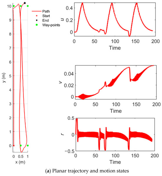
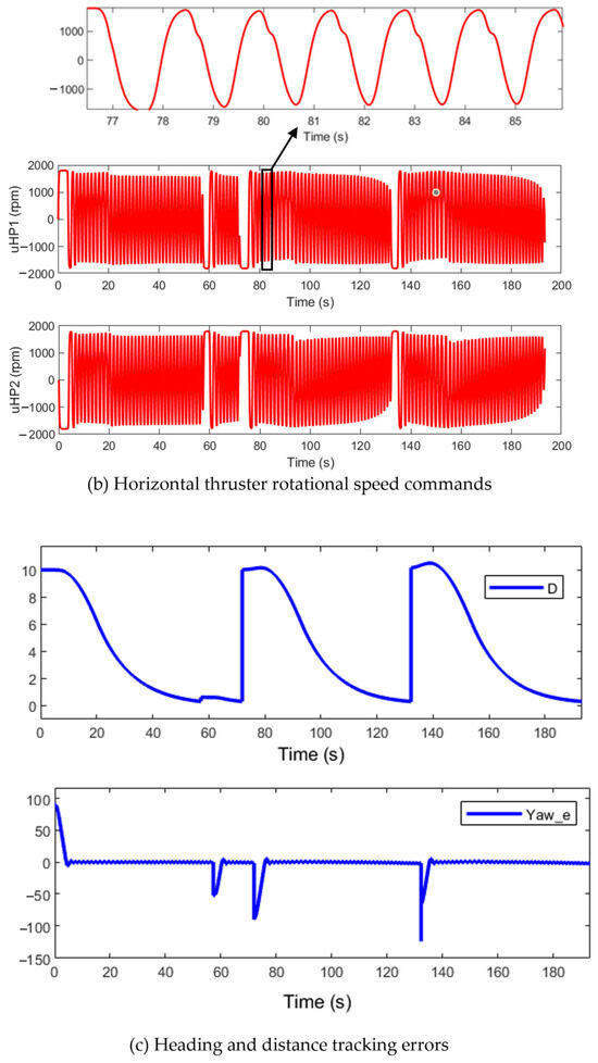
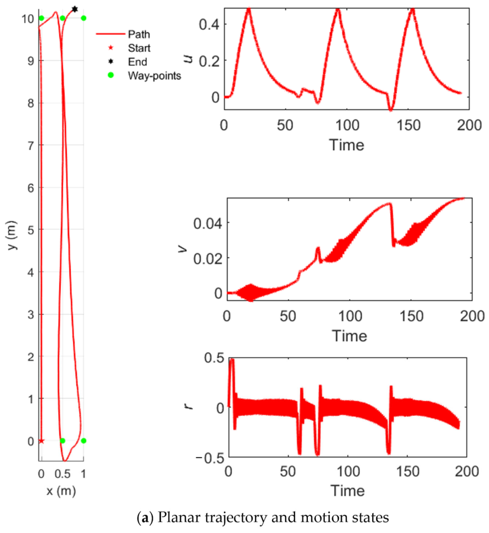
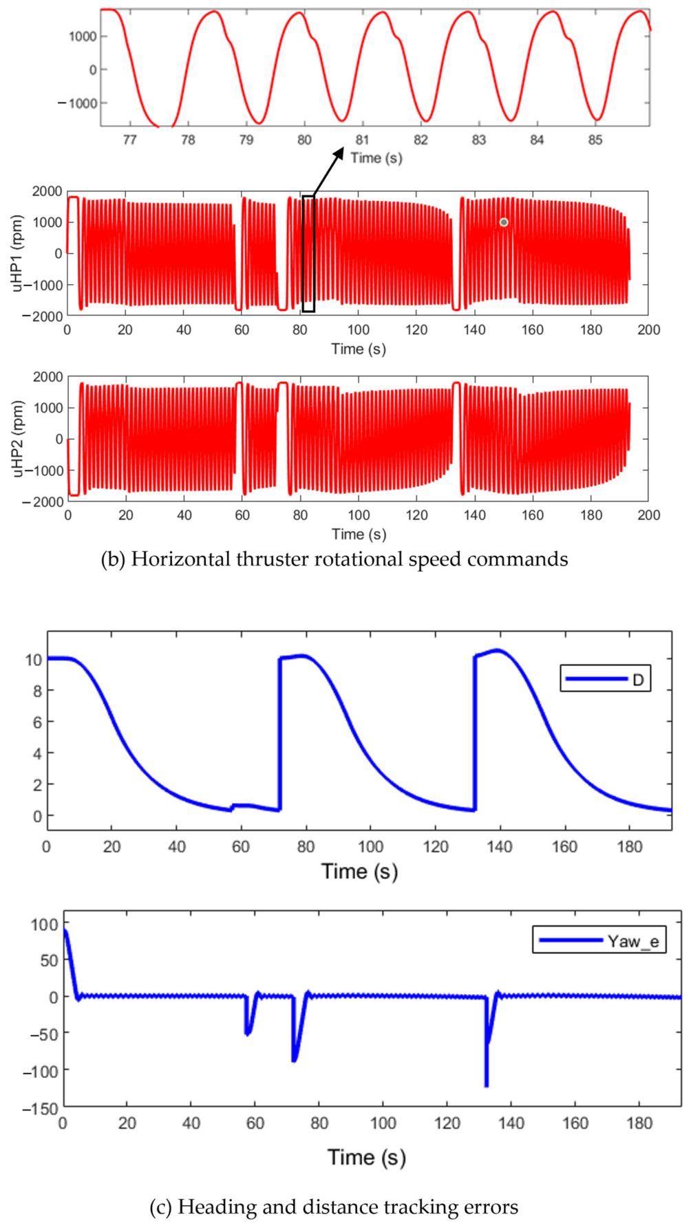
To evaluate the performance of the proposed closed-loop guidance and control framework under nominal operational conditions, a round-trip mission encompassing five sequential waypoints is designated as the simulation benchmark, spanning a total trajectory length of 16 BL (21 m). The sequence of waypoints is shown in Table 1. The comprehensive control performance is illustrated in Figure 12; specifically, Figure 12a–c delineate the time-histories of the robot’s kinematics, the allocated thruster speed commands, and the evolution of tracking errors, respectively. From the simulation results, it can be seen that the PD control law enables the robot to achieve waypoint tracking control within the allowable radius and the thruster rotational speed constraints. In the simulations, the thruster dynamics were modeled with a rotational speed saturation of ±2000 rpm and a minimum response time of 0.02 s (50 Hz), consistent with the typical specifications of the commercially available T200 thrusters commonly used in underwater vehicles. The rpm commands from the waypoint-following tests were recorded and checked against these limits, and as shown in Figure 12b, all commanded values remained strictly within the allowable range throughout the entire maneuver. However, the nonlinearity of the actuator model, combined with the instantaneous command variations at discrete waypoint switching instants, causes fluctuations in the PD outputs and thrust allocation. While this is a normal consequence of the switching logic, it remains within the actuator limits. Future mitigation could include command filtering or smooth trajectory planning to reduce such transient effects.
Table 1.
Waypoint Sequence.
Figure 12.
Waypoint following control results of the underwater cleaning robot.
To quantitatively evaluate the waypoint-tracking control performance, the following metrics are extracted from the simulation results: the minimum heading tracking error is approximately 0.08°, the settling time (within ±5° error band) is about 5 s, and the minimum waypoint distance tracking error is approximately 0.13 m (i.e., the waypoint switching radius). In addition, to provide a more comprehensive assessment of the overall tracking performance, we further compute the maximum error, root-mean-square error (RMSE), and integral absolute error (IAE) for both position and heading errors. Specifically, the maximum position error and maximum heading error are approximately 10 m and 90°, respectively, corresponding to the inter-waypoint distance and heading difference; the RMSE of the position error D is 5.63 m, and the RMSE of the heading error is 14.14°; the IAE of D is 804.31 m·s, and the IAE of the heading error is 803.67 deg·s. The reported maximum error occur transiently immediately after waypoint switching, due to abrupt changes in the desired heading, these values do not reflect the steady-state tracking accuracy. Together with the basic transient indicators, these results demonstrate that the proposed guidance and control strategy achieves satisfactory waypoint tracking under the specified operational constraints.
5. Conclusions
This paper presents a systematic study on the mechanical analysis and motion control of an underwater cleaning robot operating on jacket columns. The primary conclusions are as follows:
- (1)
- By analyzing the robot’s stationary operational states, the main failure modes of the robot in a stationary state were identified. Taking a typical column with a diameter of 2000 mm and a horizontal inclination angle of 90° as the object, the mechanical condition for the robot’s stable climbing was derived: . Assuming the equivalent gravity is neutralized by buoyancy materials, the constraint relationship between the adhesion force and the propulsive force simplifies to , which provides a design basis for the parameter matching of the adhesion and driving systems.
- (2)
- Leveraging the developed six-degree-of-freedom dynamic model, an open-loop maneuvering simulation platform was constructed in the MATLAB/Simulink environment. Simulations reveal that within the rotational speed range of 500–3000 rpm, the robot’s straight-line speed can reach 0.233–1.601 BL/s, and the maximum steady-state thrust of the horizontal thrusters is approximately 80 N, corresponding to an upper limit of the required adhesion force of about 106.4 N. This platform can effectively predict the robot’s underwater motion response, laying a foundation for subsequent closed-loop control design.
- (3)
- To address the planar waypoint tracking mission, a closed-loop control system integrating line-of-sight (LOS) guidance, a waypoint switching strategy with an acceptance radius, and a PD control law was designed, and a complete simulation platform. A complete simulation framework, including the nonlinear mapping from control forces to thruster commands, was established. The waypoint-following simulation results show that under the thruster rotational speed constraints and the allowable radius condition of , the robot successfully navigates through five designated waypoints, with position and heading errors converging well, thereby verifying the effectiveness of the proposed guidance and control strategy.
In summary, the mechanical analysis model, open-loop simulation platform, and closed-loop motion control strategy established in this paper can provide a theoretical basis and technical reference for the stable operation and autonomous navigation control of underwater jacket cleaning robots. It is important to acknowledge that the closed-loop simulations presented in this work are performed in an idealized environment. Several factors that are present in real-world operations, including sensor noise, communication delays, actuator saturations, time-varying ocean currents, and model parameter uncertainties, have been deliberately omitted to isolate the core theoretical contributions. These practical issues, however, constitute essential directions for our ongoing and future research. Future work will focus on incorporating current observers, actuator saturations, sensor noise, and model parameter uncertainties to further enhance the engineering practicality and robustness of the control strategy in real underwater operating environments.
Author Contributions
Conceptualization, J.Y., W.S. and X.L.; methodology, W.S. and Y.Z. (Ying Zhang); software, Y.Z. (Yupeng Zou) and X.Y.; validation, J.Y., W.S. and X.Y.; formal analysis, J.Y. and Y.Z. (Ying Zhang); investigation, Y.Z. (Ying Zhang) and Y.Z. (Yupeng Zou); resources, J.Y. and X.L.; data curation, W.S. and X.L.; writing—original draft preparation, J.Y., W.S. and Y.Z. (Yupeng Zou); writing—review and editing, X.C., Y.Z. (Yupeng Zou) and Y.M.; visualization, X.C.; supervision, Y.M.; project administration, Y.Z. (Yupeng Zou); funding acquisition, Y.Z. (Yupeng Zou). All authors have read and agreed to the published version of the manuscript.
Funding
This research was funded by the Fundamental Research Funds for the Central Universities, grant number 26CX02012A; and the Research Funds of Guangdong Power Grid Co., Ltd., grant number GDKJXM20240661. The APC was funded by the Fundamental Research Funds for the Central Universities, grant number 26CX02012A.
Institutional Review Board Statement
Not applicable.
Informed Consent Statement
Not applicable.
Data Availability Statement
The original contributions presented in this study are included in the article. Further inquiries can be directed to the corresponding author.
Conflicts of Interest
Junwen Yao, Xionggang Li, Ying Zhang and Xiao Yue were employed by the Electric Power Research Institute of Guangdong Power Grid Co., Ltd. Wenxing Sun was employed by Guangdong Power Grid Co., Ltd. The remaining authors declare no conflicts of interest.
Appendix A
The robot adheres to the surface of the offshore jacket through the thrust generated by vertically mounted thrusters and the magnetic adhesion force provided by magnetic adhesion drive wheels. It moves along the jacket surface driven by the magnetic adhesion drive wheels, while the cleaning discs mounted on the robot perform the cleaning operation. The robot mainly consists of a magnetic adhesion wheeled chassis, cleaning discs, thruster assemblies, and a control compartment. The total mass of the robot is approximately m = 150 kg, and its principal inertia tensor is I = diag{61.26, 54.63, 96.83} kg·m2 The overall dimensions are approximately L × W × H = 1.3 m × 1.2 m × 0.4 m. The simplified virtual prototype model and the detailed dimensional drawing are shown in Appendix A Figure A1 and Figure A2, respectively. The left and right horizontal thrusters are denoted as HP1 and HP2, respectively; the left and right vertical thrusters are denoted as VP1 and VP2, respectively; the left and right front wheels are denoted as FW1 and FW2, respectively; and the left and right rear wheels are denoted as BW1 and BW2, respectively.
Four T200 propeller thrusters with forward-rotation propellers are used to provide horizontal thrust and vertical thrust, the latter serving as the adhesion force. The wheel diameter and width of the wheeled chassis are 0.5 m and 0.1 m, respectively. The positions of the thrusters and drive wheels relative to the robot’s center of gravity are listed in Appendix A Table A1.
Figure A1.
Simplified virtual prototype model of the underwater cleaning robot.
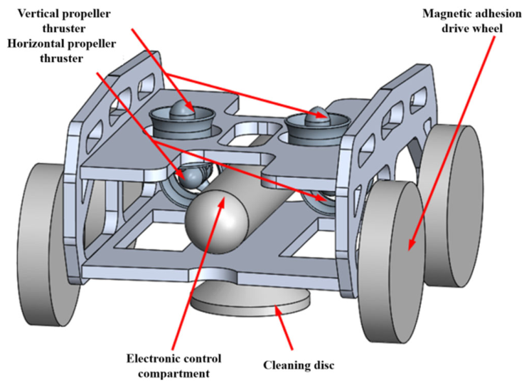
Figure A2.
Dimensional drawing of the underwater cleaning robot.
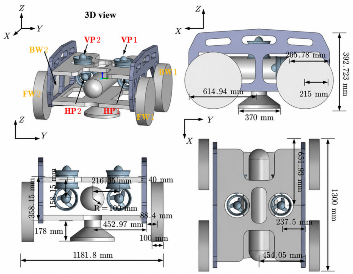
Table A1.
Coordinates of the rotating-domain center with respect to the robot center of gravity.
Appendix B
The appendix provides the numerical values of the hydrodynamic forces and moments, and the coefficient matrices for the robot model mentioned in Equation (3) of this paper.
The hydrodynamic forces and moments can be further divided into three components: added-mass forces and moments, damping forces and moments, and hydrostatic restoring forces and moments caused by gravity and buoyancy.
The added-mass forces and moments are expressed as , By approximating the robot as a regular geometric body, the following expression can be obtained:
where are the added-mass coefficients, which are obtained through the CFD simulations.
The damping force is one of the fundamental components of the fluid forces acting on the robot during its motion. The viscous resistance in six degrees of freedom is described using the second-order Taylor series expansion of the Morison equation, with higher-order terms neglected. Accordingly, the viscous-force coefficient matrix can be expressed as:
Similarly, the damping-force coefficients involved are also obtained through CFD simulations.
Gravity and buoyancy are referred to as hydrostatic restoring forces in fluid mechanics, acting at the center of gravity and the center of buoyancy of the underwater cleaning robot, respectively. Moreover, since the center of gravity and the center of buoyancy do not coincide, when the underwater cleaning robot undergoes pitch and roll motions, gravity and buoyancy no longer act along the same vertical line, thereby generating restoring moments. Therefore, the six-dimensional restoring force vector can be obtained as:
Here, and are the vectors of gravity and buoyancy in the body-fixed frame, and are the vectors of the center of gravity and buoyancy in the body-fixed frame.
Through CFD simulations employing overset grids, moving reference frames, and forced oscillation techniques [25], the damping coefficients and added-mass coefficients are identified for each degree of freedom, as shown in Appendix B Table A2. In particular, the added-mass coefficients were determined via the forced oscillation method using transient CFD simulations in Fluent on a simplified 3D model of the robot, where sinusoidal periodic motions with very small amplitudes were imposed in each degree of freedom, and the coefficients were calculated from the forces and accelerations at the instants when the motion velocity reached zero; the damping coefficients, on the other hand, were obtained through steady-state towing simulations in Fluent over a flow velocity range of 0.1 to 1.0 m/s, with numerical fitting performed along each degree of freedom to yield both linear and quadratic damping coefficients.
Table A2.
Hydrodynamic coefficient values.
Appendix C
The thruster model of the robot is presented in this section.
Under conventional motion, the robot uses only the propeller thrusters as actuators for motion driving and control, while the magnetic adhesion drive wheels remain inactive. The driving forces and moments generated by different actuators can be expressed as:
where denotes the resultant forces and moments generated by the left and right horizontal propeller thrusters, and denotes the thrust forces and moments generated by the two vertical propeller thrusters.
The thrust of the propeller thruster is generated by the rotation of the propeller driven by the motor. A series of simulation data for the thrust and torque can be obtained through CFD simulations, based on which the thrust coefficient and torque coefficient are calculated using Equation (A7).
where denotes the fluid density, denotes the rotational speed of the propeller, and denotes the propeller diameter. The simulation data are analyzed using least-squares fitting to obtain the relationship curves between the advance coefficient and and . The advance coefficient is calculated as follows, where the rotational speed is expressed in rev/s:
where denotes the translational velocity of the thruster.
Taking the force and moment generated by the right horizontal propeller thruster as an example, its thrust can be expressed as , and the corresponding moment is given by Here, denotes the position vector from the origin of the body-fixed frame to the thrust application center of the right horizontal propeller thruster, and represents the moment generated by the thrust about the body-fixed frame. Since , the propeller-induced torque can be neglected. Therefore, the resultant driving forces and moments generated by the left and right horizontal propeller thrusters can be expressed as:
where and denote the rotational speeds of the left and right horizontal propeller thrusters, respectively. Similarly, the thrust forces and moments provided by the vertical thrusters can be expressed as follows:
References
- Hadžić, N.; Jovanović, I.; Vladimir, N. Biofouling of ships and offshore structures: Research trends and future pathways. Ocean Eng. 2026, 347, 123988. [Google Scholar] [CrossRef] [Scilit]
- Poozesh, P.; Nieto, F.; Fernández, P.M.; Ríos, R.; Díaz-Casás, V. Biofouling on offshore wind energy structures: Characterization, impacts, mitigation strategies, and future trends. J. Mar. Sci. Eng. 2025, 13, 1363. [Google Scholar] [CrossRef] [Scilit]
- Schoefs, F.; Bakhtiari, A.; Ameryoun, H. Evaluation of Hydrodynamic Force Coefficients in Presence of Biofouling on Marine/Offshore Structures, a Review and New Approach. J. Mar. Sci. Eng. 2022, 10, 558. [Google Scholar] [CrossRef] [Scilit]
- Vuong, T.; McKinley, A.; Kaur, P. Understanding biofouling and contaminant accretion on submerged marine structures. npj Mater. Degrad. 2023, 7, 50. [Google Scholar] [CrossRef] [Scilit]
- Xu, D.; Gu, T.; Lovley, D.R. Microbially mediated metal corrosion. Nat. Rev. Microbiol. 2023, 21, 705–718. [Google Scholar] [CrossRef] [Scilit] [PubMed]
- Lin, S.; Bi, H.; Weinell, C.E.; Dam-Johansen, K. Submerged surfaces exposed to marine biofouling—Experimental investigation of cleaning parameters effectiveness. Prog. Org. Coat. 2022, 172, 107097. [Google Scholar] [CrossRef] [Scilit]
- Ahn, J.; Yan, K.; Bazher, S.A.; Oh, J.; Seo, D.; Cho, S.-G.; Kim, H. Evaluation of Influencing Factors in Cleaning Performance for Bio-Fouling Removal Based on High-Pressure Water Jets. J. Mar. Sci. Eng. 2024, 12, 1086. [Google Scholar] [CrossRef] [Scilit]
- Yuan, T.-P.; Huang, X.-H.; Hu, Y.; Wang, S.-M.; Tao, Q.-Y.; Pang, G.-L. Aquaculture net cleaning with cavitation improves biofouling removal. Ocean Eng. 2023, 285, 115241. [Google Scholar] [CrossRef] [Scilit]
- Park, D.; Han, J.-B.; Yeu, T.; Cho, S.-G.; Kim, S.; Kim, H.; Lee, Y. Development of an Autonomous Cleaning Robot with a Hydraulic Manipulator Arm for the Cleaning of Niche Areas of a Ship Hull. J. Mar. Sci. Eng. 2023, 11, 973. [Google Scholar] [CrossRef] [Scilit]
- Chen, L.; Cui, R.; Yan, W.; Xu, H.; Zhao, H.; Li, H. Design and climbing control of an underwater robot for ship hull cleaning. Ocean Eng. 2023, 274, 114024. [Google Scholar] [CrossRef] [Scilit]
- Jiao, S.; Zhang, X.; Sun, L.; Shi, Y.; Zhang, M. Structural Design and Horizontal Wave Force Estimation of a Wall-Climbing Robot for the Underwater Cleaning of Jackets. J. Mar. Sci. Eng. 2024, 12, 1612. [Google Scholar] [CrossRef] [Scilit]
- Yang, C.; Liu, S.; Su, H.; Zhang, L.; Xia, Q.; Chen, Y. Review of underwater adsorptive-operating robots: Design and application. Ocean Eng. 2024, 294, 116794. [Google Scholar] [CrossRef] [Scilit]
- Li, C.; Hu, Z.; Zhang, D.; Wang, X. System Identification and Navigation of an Underactuated Underwater Vehicle Based on LSTM. J. Mar. Sci. Eng. 2025, 13, 276. [Google Scholar] [CrossRef] [Scilit]
- Villa, J.; Vallicrosa, G.; Aaltonen, J.; Ridao, P.; Koskinen, K.T. Model-Validation and Implementation of a Path-Following Algorithm in an Autonomous Underwater Vehicle. Appl. Sci. 2021, 11, 11891. [Google Scholar] [CrossRef] [Scilit]
- Bao, H.; Zhu, H. Modeling and Trajectory Tracking Model Predictive Control Novel Method of AUV Based on CFD Data. Sensors 2022, 22, 4234. [Google Scholar] [CrossRef] [Scilit] [PubMed]
- Du, P.; Yang, W.; Chen, Y.; Huang, S.H. Improved indirect adaptive line-of-sight guidance law for path following of under-actuated AUV subject to big ocean currents. Ocean Eng. 2023, 281, 114729. [Google Scholar] [CrossRef] [Scilit]
- Xu, Y.F.; Wan, L.; Zhang, Z.; Chen, G. Robust adaptive path following control of autonomous underwater vehicle with uncertainties and communication bandwidth limitation. Ocean Eng. 2023, 287, 115895. [Google Scholar] [CrossRef] [Scilit]
- Miao, J.; Liu, W.; Peng, C.; Sun, X. Robust path-following control of the underactuated AUV with multiple uncertainties using combined UDE and UKF. J. Mar. Sci. Technol. 2023, 28, 804–818. [Google Scholar] [CrossRef] [Scilit]
- Meng, F.; Liu, A.; Hu, Y.; Ren, D.; Liu, Y.; Zhang, X. A Control Method for Path Following of AUVs Considering Multiple Factors Under Ocean Currents. J. Mar. Sci. Eng. 2024, 12, 2045. [Google Scholar] [CrossRef] [Scilit]
- Wang, Y.; Hou, Y.; Lai, Z.; Cao, L.; Hong, W.; Wu, D. An adaptive PID controller for path following of autonomous underwater vehicle based on Soft Actor–Critic. Ocean Eng. 2024, 307, 118171. [Google Scholar] [CrossRef] [Scilit]
- Breivik, M.; Fossen, T.I. Guidance-based path following for autonomous underwater vehicles. In Proceedings of the OCEANS 2005 MTS/IEEE, Washington, DC, USA, 17 September 2005. [Google Scholar] [CrossRef] [Scilit]
- Ataei, M.; Yousefi-Koma, A. Development of a three-dimensional guidance system for long-range maneuvering of a miniature autonomous underwater vehicle. China Ocean Eng. 2014, 28, 843–856. [Google Scholar] [CrossRef] [Scilit]
- Rizk, H.; Chaibet, A.; Kribèche, A. Model-Based Control and Model-Free Control Techniques for Autonomous Vehicles: A Technical Survey. Appl. Sci. 2023, 13, 6700. [Google Scholar] [CrossRef] [Scilit]
- He, Z.; Zhao, L. A Simple Attitude Control of Quadrotor Helicopter Based on Ziegler-Nichols Rules for Tuning PD Parameters. Sci. World J. 2014, 2014, 280180. [Google Scholar] [CrossRef] [Scilit] [PubMed]
- Xue, G.; Bai, F.; Guo, L.; Ren, P.; Liu, Y. Research on the effects of complex terrain on the hydrodynamic performance of a deep-sea fishlike exploring and sampling robot moving near the sea bottom. Front. Mar. Sci. 2023, 10, 1091523. [Google Scholar] [CrossRef] [Scilit]

Disclaimer/Publisher’s Note: The statements, opinions and data contained in all publications are solely those of the individual author(s) and contributor(s) and not of MDPI and/or the editor(s). MDPI and/or the editor(s) disclaim responsibility for any injury to people or property resulting from any ideas, methods, instructions or products referred to in the content. |
© 2026 by the authors. Licensee MDPI, Basel, Switzerland. This article is an open access article distributed under the terms and conditions of the Creative Commons Attribution (CC BY) license.