


Abstract
Smart sensor networks for environmental monitoring require accurate and continuous estimation of key variables such as temperature, humidity, and wind speed; however, physical sensor deployments are frequently limited by high costs, hardware failures, and data quality degradation, while existing virtual sensor approaches rely on single-model architectures that lack explicit uncertainty modeling and fail to capture the complex non-linear dynamics of real-world IoT time-series data. This paper proposes VAS-DPFF, a virtual augmented sensor framework based on deterministic and probabilistic feature fusion, which contributes a principled integration of well-established deterministic and probabilistic techniques within a unified AIoT-compatible virtual sensing architecture. The framework integrates: (i) a deterministic pipeline comprising temporal encoding, rolling statistics, and mutual information-based feature selection; (ii) a probabilistic pipeline employing Bayesian Ridge Regression (BRR) and Gaussian Process Regression (GPR) to generate uncertainty-aware synthetic features; and (iii) an early feature-level fusion strategy feeding an XGBoost regression model augmented with Gaussian noise injection. Experiments on 84,582 time-series records from a nine-station IoT environmental monitoring network in Gwacheon City, South Korea, demonstrate strong multi-target prediction performance: temperature RMSE = 0.811 °C, R2 = 0.973; humidity RMSE %, R2 = 0.964; and wind speed RMSE m/s, R2 = 0.798, representing RMSE reductions of 61.2%, 60.7%, and 62.3% over the existing method, respectively. Comprehensive ablation studies, sensitivity analysis, and augmentation validation confirm that the proposed integration of deterministic and probabilistic features yields consistent and practically valuable improvements in virtual sensing performance suitable for AIoT-enabled smart sensor network deployments across multiple environmental monitoring targets.
1. Introduction
Environmental monitoring is fundamental to a wide range of applications including smart city development, climate analysis, precision agriculture, industrial process control, and public health management [1,2]. Accurate and continuous measurement of key variables such as temperature, humidity, and wind speed underpins system reliability and informed decision-making across these domains [3]. Physical sensors remain the dominant measurement modality; however, they are frequently associated with high installation and maintenance costs, hardware failure, sensor drift, calibration requirements, and noise-induced data corruption [4,5]. These challenges degrade system performance and restrict scalability, particularly in large-scale or resource-constrained deployment scenarios.
Virtual sensing has emerged as a promising alternative, estimating target variables through data-driven models trained on correlated, readily available measurements [6]. Despite its advantages in flexibility and cost efficiency, achieving high prediction accuracy across multiple environmental targets remains challenging. Existing virtual sensor methods predominantly adopt single-model architectures [7] that are insufficient for simultaneously capturing global temporal patterns, local fluctuations, and stochastic variability inherent in environmental time-series data. Furthermore, real-world environmental datasets are typically characterized by limited sample sizes, high temporal variability, measurement noise, and irregular sampling intervals, all of which collectively hinder model generalization [8].
1.1. Motivation and Problem Statement
Recent advances in virtual sensing have explored deep learning architectures, feature engineering pipelines, and hybrid modeling strategies [9,10,11]. While these approaches have demonstrated notable improvements, four persistent limitations motivate the present work. First, most methods rely on a limited and homogeneous feature set, restricting the model’s ability to capture the full spectrum of environmental dynamics [12]. Second, the majority of existing models lack explicit uncertainty quantification mechanisms, reducing reliability in stochastic real-world environments [13]. Third, inadequate handling of temporal dependencies limits effectiveness in dynamic and non-stationary conditions [14]. Fourth, deep learning-based approaches typically require large labeled datasets that are often unavailable in environmental monitoring deployments [15].
1.2. Research Challenges
Building an effective virtual augmented sensor framework involves the following non-trivial challenges: (i) designing a rich feature space that captures both deterministic temporal structure and stochastic variability; (ii) integrating probabilistic methods for explicit uncertainty quantification without excessive computational overhead; (iii) generating statistically consistent synthetic data to address training data scarcity; (iv) effectively fusing heterogeneous deterministic and probabilistic feature representations; and (v) ensuring robust generalization across multiple target variables and diverse temporal conditions.
1.3. Main Contributions
The primary contribution of this work lies in the principled and structured integration of well-established deterministic and probabilistic techniques within a unified virtual sensing architecture, rather than in the proposal of a fundamentally new algorithmic paradigm. The specific contributions are as follows:
- Unified Multi-Pipeline Architecture: A systematic integration of deterministic feature engineering and probabilistic synthetic data generation via BRR and GPR within a single cohesive pipeline, overcoming the limitations of single-model virtual sensing approaches.
- Early Feature-Level Fusion: Deterministic and uncertainty-aware probabilistic features are combined at the input level, enabling XGBoost to jointly exploit global temporal patterns and local stochastic variations inaccessible to single-pipeline strategies.
- Multi-Target Empirical Validation: Experiments on 84,582 records from nine IoT monitoring stations in Gwacheon City, South Korea, covering temperature, humidity, and wind speed with ablation studies, sensitivity analysis, and state-of-the-art comparisons.
- Demonstrated Performance: RMSE reductions of 61.2%, 60.7%, and 62.3% over the existing method with R2 = 0.973, , and for temperature, humidity, and wind speed, respectively.
1.4. Paper Organization
Section 2 reviews related work. Section 3 presents the VAS-DPFF methodology. Section 3 describes the VAS-DPFF methodology, with Section 3.6 covering the algorithmic specification. Section 4 details the experimental setup. Section 5 presents experimental results. Section 6 provides discussion and analysis. Section 7 concludes the paper.
2. Related Work
Virtual sensing has emerged as a scalable and cost-effective alternative to physical sensors across industrial process monitoring, smart buildings, precision agriculture, and environmental monitoring [16,17]. This section reviews twenty representative works organized into five thematic categories and concludes with a comparative analysis identifying the research gaps motivating the proposed VAS-DPFF framework.
2.1. Deep Learning-Based Virtual Sensors
Deep learning has been widely adopted for virtual sensor modeling due to its capacity to learn complex non-linear mappings directly from raw data. Yuan et al. [18] proposed a Supervised Hybrid CNN-LSTM (SDCNN-LSTM) for nonlinear dynamic soft sensing, injecting quality variables into each hidden layer with 1D→2D data augmentation, outperforming LSTM, NARX, and SLSTM baselines on penicillin fermentation and debutanizer processes. Wang et al. [19] introduced STCIM, a spatio-temporal consistent and interpretable soft sensor integrating physics-informed latent space loss with a far-topological alignment block, demonstrating superior generalization across varying operating conditions in coal-fired power plants. Liu et al. [20] proposed SA-BiLSTM, combining bidirectional LSTM with supervised temporal attention and a moving window quality injection strategy, outperforming LSTM, SLSTM, and BiLSTM for nonlinear industrial quality prediction. He et al. [21] applied Deep Operator Networks (DeepONet) as virtual sensors for nuclear reactor digital twins, mapping operational inputs to spatially distributed thermal-hydraulic parameters 1400× faster than CFD simulation without retraining. Götz et al. [22] introduced the first unified multi-task foundation model for virtual sensors, simultaneously predicting diverse virtual sensors with cross-task synergy while maintaining computational efficiency for edge deployment. Despite their strong performance, deep learning methods share critical limitations: they require large labeled datasets, involve high computational complexity, offer limited interpretability, and underperform in data-scarce environments [18,20,21].
2.2. Machine Learning and Feature Engineering Approaches
Classical machine learning methods combined with systematic feature engineering offer computational efficiency and interpretability advantages over deep learning. Wu et al. [23] developed feature selection-based ML for Distributed Model Predictive Control (DMPC), combining filter, wrapper, and embedded selection with reduced-order RNN models for reactor-separator processes, achieving desired closed-loop performance with improved computational efficiency. Liu et al. [24] proposed NPER/SNPER/LW-SNPER, neighborhood-preserving embedding regression methods with sparse elastic-net regularization for semiconductor manufacturing, outperforming global regression and preserving local manifold structure in high-dimensional settings. Xu et al. [25] introduced FS-NSVR, a novel feature selection method for nonlinear SVR via mixed-integer programming with an alternate iterative greedy algorithm, selecting fewer features than L1-SVR/Lp-SVR with comparable RMSE and faster runtime. Curreri et al. [16] provided a systematic review of filter, wrapper, embedded, and causal MI-based variable selection methods for data-driven soft sensors, confirming that causal model-inspired approaches outperform correlation-based methods in generalization. These methods generally assume stationary data distributions, limiting their effectiveness in dynamic and non-stationary environmental monitoring scenarios [16,24,25].
2.3. Control-Theoretic and Semi-Supervised Methods
Control-theoretic approaches provide theoretically grounded virtual sensor designs with formal stability guarantees. Zhirabok et al. [26] designed robust virtual sensors for nonlinear discrete-time systems using Jordan canonical forms and algebra of functions, achieving minimal-dimension disturbance-insensitive observers validated on a three-tank benchmark. In a related work, Zhirabok et al. [27] addressed virtual sensor design for dynamic systems with non-smooth nonlinearities (backlash, saturation, hysteresis) using a logic-dynamic approach, providing a general solution framework with reduced computational complexity. While these methods offer strong theoretical guarantees, they require prior system knowledge and are restricted to systems where canonical algebraic structures are derivable.
Zhao et al. [28] proposed LPSCN, a semi-supervised stochastic configuration network with locality-preserving regularization that leverages both labeled and unlabeled training samples, outperforming standard SCN on RMSE and R2 for sulfur recovery and debutanizer column industrial processes. Curreri et al. [17] reviewed sensor virtualization with AI/ML in Industry 4.0 contexts, demonstrating the viability of ML-based virtual sensors as cost-effective replacements across wastewater treatment, energy management, and environmental monitoring domains, while identifying data quality dependency and black-box interpretability as persistent challenges.
2.4. Building Systems and Environmental Monitoring
Virtual sensing methods applied to building energy systems and environmental monitoring represent the domain most directly relevant to the proposed VAS-DPFF framework. Li et al. [29] proposed a gray-box virtual sensor for room temperature prediction integrating heat transfer physics with multiple linear regression and a nonlinear GRG algorithm with physical constraints, demonstrating that single-condition training generalizes to multiple HVAC modes with better extrapolation than pure black-box models. Zhang et al. [30] introduced ISIC (In-situ Selective Incremental Calibration) for HVAC temperature sensor fault-tolerant control using Bayesian inference and PCA with EnergyPlus-Python co-simulation, achieving 6.8% energy reduction after thermostat fault-tolerant control. Shen and Pan [31] developed a hybrid feature selection framework for indoor temperature prediction in large-space buildings combining Max-min Transfer Entropy in a filter stage with a GRU wrapper and lifecycle cost referee via TRNSYS simulation, identifying cost-efficient feature subsets under different prediction horizons. The most directly related work to the present study is VSG-SGL [32], which combines Sparse GPR and Bayesian Ridge Regression with VAE/CTGAN generative augmentation, Isolation Forest anomaly detection, and KDE distributional validation for meteorological variable prediction (temperature, humidity, wind) across South Korean cities—the same geographic context as the proposed VAS-DPFF framework. VSG-SGL demonstrates that VAE-augmented virtual sensors are most stable, with SGPR wind speed MAE improving from 0.1848 to 0.1604 with VAE augmentation and BRR wind direction RMSE reducing from 0.1842 to 0.1726. However, VSG-SGL relies on CTGAN augmentation that degrades performance for some variables, does not integrate deterministic feature engineering or MI-based selection, and lacks a unified early feature-level fusion strategy. Ahmadnia et al. [33] addressed building sensor coverage through dual integer linear programming models with a Leader-Follower bi-level approach, achieving optimal cost-coverage balance for smart building air quality sensor placement.
2.5. Data Augmentation and Graph-Based Models
Saab et al. [34] proposed a VAE-GAN augmentation pipeline for vertebral compression fracture detection using CTSpine1K synthetic pre-training with DCGAN, VAE, and VAE-GAN comparison, achieving FID 5× lower than alternatives and improving classification accuracy from 73% to 89%. While demonstrating strong augmentation performance, the approach requires large synthetic pre-training datasets and complex training procedures. Zhao et al. [35] developed HTGNN (Heterogeneous Temporal Graph Neural Network) for virtual sensing in complex systems, treating multi-modal sensor nodes as distinct graph node types with exogenous variable context integration, significantly outperforming existing methods for bearing load and bridge live load prediction under highly varying operating conditions with publicly released code. Despite their representational power, graph-based models require domain-specific graph topology construction and suffer from scalability issues in large sensor networks.
2.6. Research Gap and Positioning
A critical synthesis of the twenty reviewed works reveals six persistent limitations that collectively motivate VAS-DPFF: (i) limited feature diversity from homogeneous representations [16,23,24]; (ii) absence of explicit uncertainty modeling [18,19,20]; (iii) dependency on large labeled datasets [18,20,21,34]; (iv) domain specificity restricting cross-environment generalization [26,27,29]; (v) high computational complexity limiting real-time deployability [21,32,35]; and (vi) single-target evaluation without multi-variable assessment [23,25,28]. No existing approach simultaneously addresses all six challenges for multi-target environmental prediction covering temperature, humidity, and wind speed. In contrast to the most closely related work VSG-SGL [32], which uses BRR and GPR but lacks deterministic feature engineering and unified fusion, the proposed VAS-DPFF framework integrates both deterministic and probabilistic pipelines through early feature-level fusion within a single scalable architecture evaluated across three targets simultaneously. Table 1 summarizes the positioning of VAS-DPFF relative to key reviewed approaches.
Table 1.
Comparative analysis of reviewed virtual sensing approaches across five design criteria. ✓ = fully addressed; ○ = partially addressed; × = not addressed.
3. Methodology
This section presents the methodology of the proposed VAS-DPFF framework. The framework is designed as a multi-stage, multi-pipeline architecture integrating deterministic feature engineering, probabilistic synthetic data generation, feature-level fusion, data augmentation, and gradient boosting regression to achieve robust multi-target prediction of temperature, humidity, and wind speed.
3.1. Framework Overview and Architecture
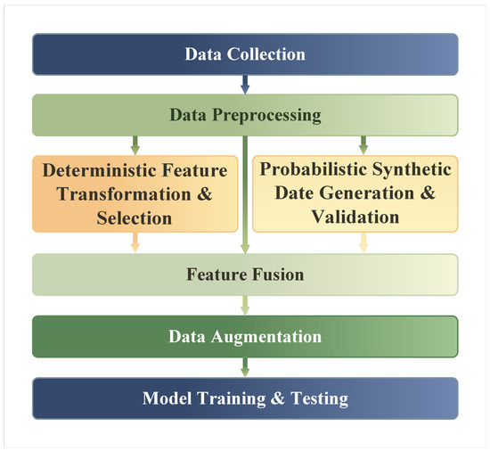
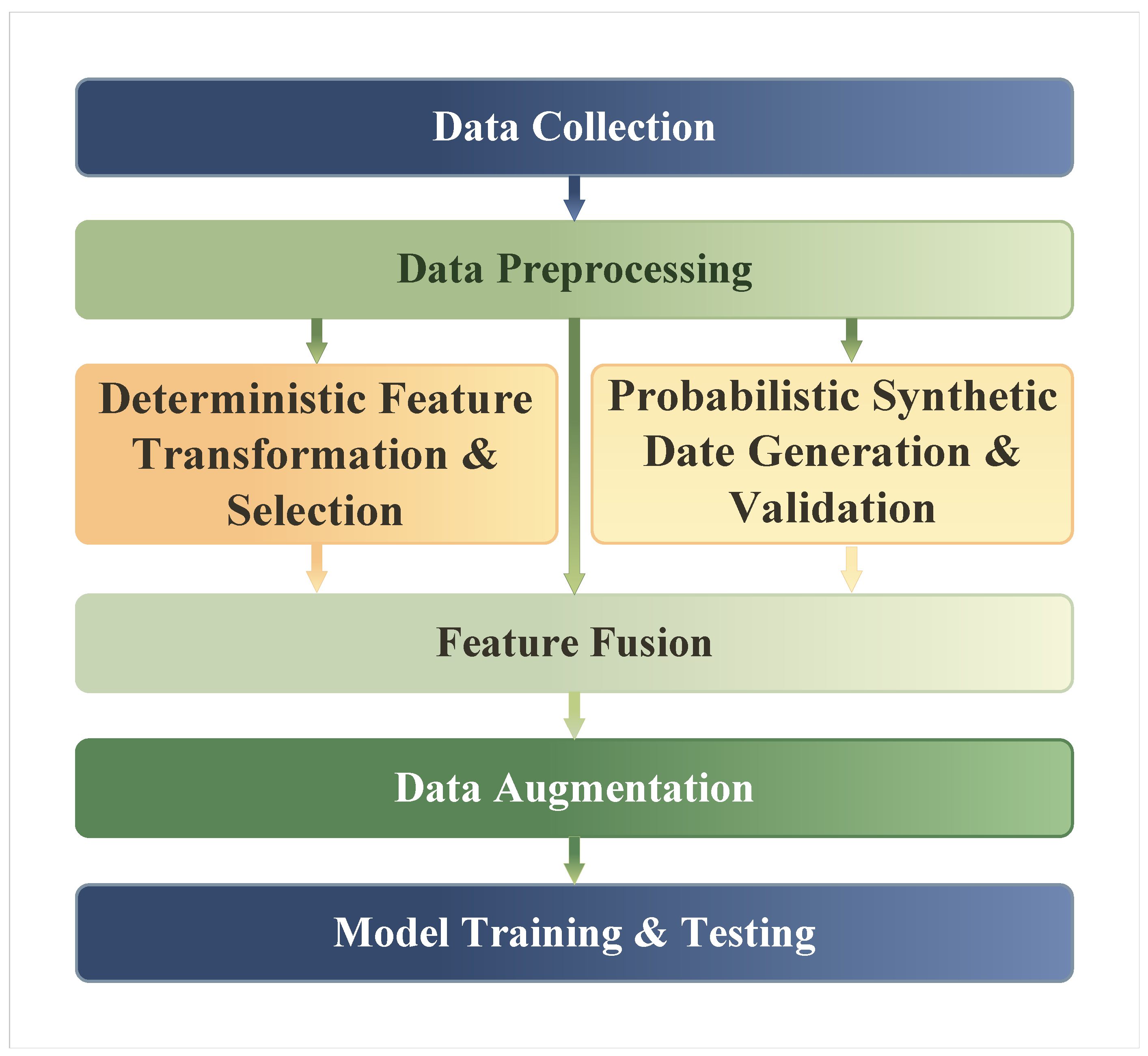
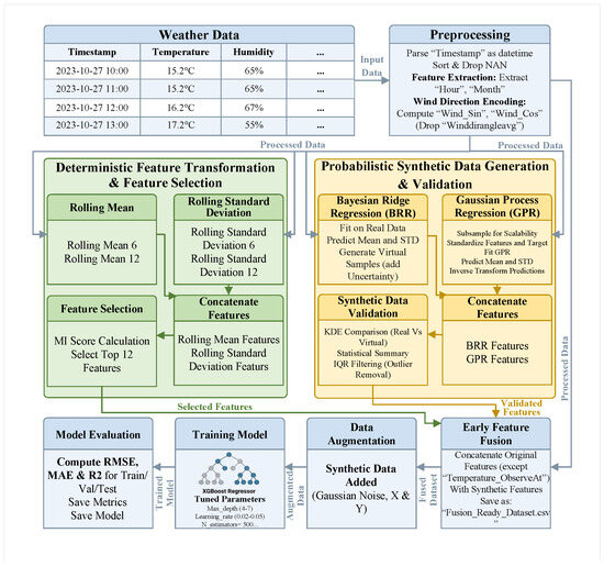
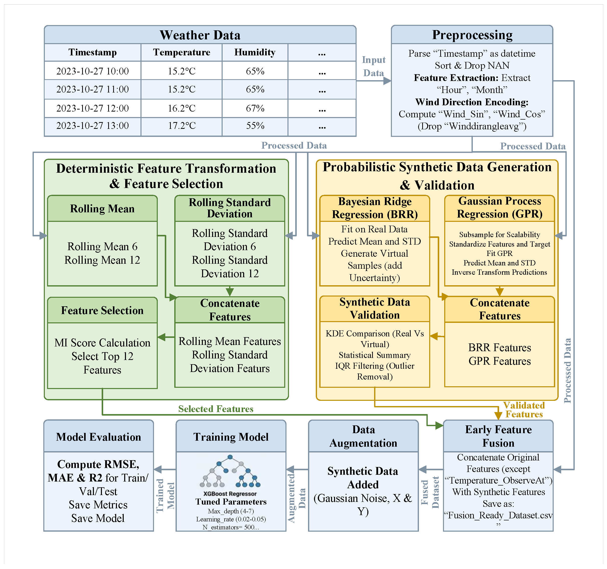
The VAS-DPFF pipeline is organized into six sequential stages: (i) data preprocessing; (ii) deterministic feature transformation and selection; (iii) probabilistic synthetic data generation; (iv) early feature-level fusion; (v) data augmentation; and (vi) model training and evaluation. Figure 1 illustrates the general framework overview and Figure 2 shows the detailed dual-pipeline architecture.
Figure 1.
General overview of the proposed VAS-DPFF framework showing the end-to-end multi-stage pipeline.
Figure 2.
Detailed dual-pipeline architecture of VAS-DPFF showing parallel deterministic and probabilistic pathways and the feature-level fusion module.
The Deterministic Pipeline performs temporal encoding, cyclic variable transformation, rolling statistical feature extraction, and mutual information-based feature selection to produce a structured compact feature set capturing global temporal patterns and short-term statistical dynamics. The Probabilistic Pipeline operates in parallel, employing BRR and GPR to generate uncertainty-aware synthetic features encoding non-linear distributional properties inaccessible to the deterministic pipeline. Both pipelines feed into an Early Fusion module that concatenates all representations into a unified high-dimensional feature vector for downstream model training.
3.2. Data Preprocessing
The preprocessing pipeline ensures temporal consistency, data quality, and foundational feature extraction across all three prediction targets. Table 2 summarizes the principal mathematical symbols used throughout this section.
Table 2.
Principal mathematical notation.
3.2.1. Temporal Structuring and Missing Value Handling
Raw timestamps are parsed to datetime format and sorted chronologically:
Records containing missing values are removed:
Temporal features are extracted to capture periodic and seasonal behavior:
3.2.2. Wind Direction Encoding
Wind direction is a circular variable requiring trigonometric encoding to eliminate angular discontinuity:
3.3. Deterministic Feature Transformation and Selection
3.3.1. Rolling Statistics
Rolling mean and standard deviation are computed over window size k for each input variable z:
Multiple window sizes capture dynamics at different temporal scales. Lag features and are additionally appended to encode short-term historical context.
3.3.2. Feature Selection via Mutual Information
Mutual information ranks features by relevance to the target variable:
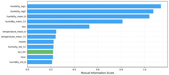
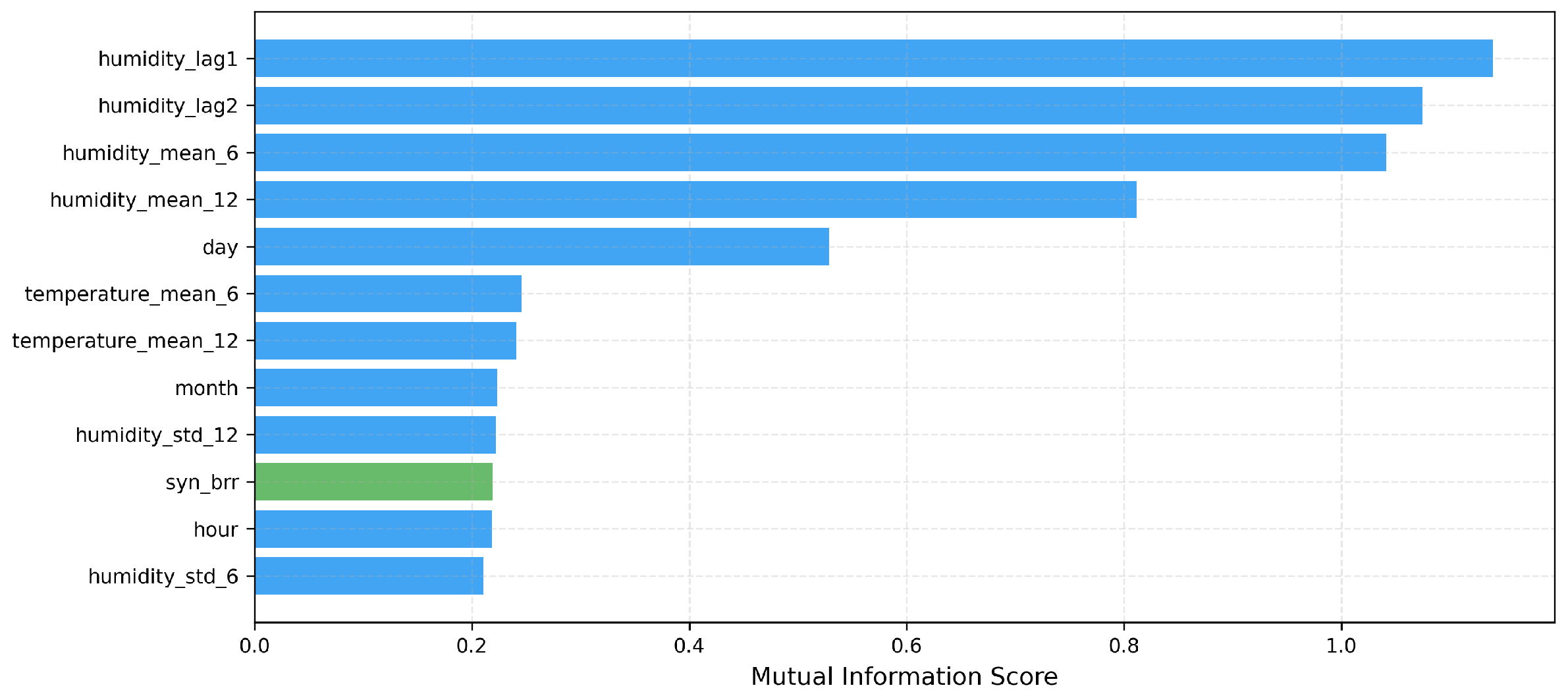
A top-K selection strategy retains the most informative features, with K set independently per target variable to balance representational capacity and dimensionality.
3.4. Probabilistic Synthetic Data Generation
3.4.1. Bayesian Ridge Regression
BRR extends linear regression with Gaussian priors over model weights, enabling principled uncertainty estimation:
where and are inferred via Empirical Bayes. The posterior is analytically Gaussian with parameters:
The predictive mean and variance are used as synthetic features in the fusion stage.
3.4.2. Gaussian Process Regression
GPR provides a non-parametric distribution-over-functions approach particularly effective for modeling non-linear local relationships:
using the RBF kernel:
The posterior predictive mean and variance for test input are:
To manage the complexity, GPR is trained on a representative subsample of inducing points per target, reducing effective complexity to . Both and are passed to the fusion stage as probabilistic synthetic features. It should be noted that this random subsampling strategy—while computationally necessary and sufficient for capturing the dominant distributional structure of the current dataset—may introduce risks of underrepresenting rare local variance patterns or minority distributional modes in significantly larger or more heterogeneous datasets. IQR-based outlier filtering and KS test validation are applied after GPR prediction as mitigation mechanisms; however, the scalability limitations of this approach are acknowledged and discussed further in Section 6.6.
3.4.3. Synthetic Data Validation
Generated synthetic features are validated through: (i) KDE comparison against real data distributions to verify alignment; (ii) statistical consistency checks (mean, variance, skewness, kurtosis); and (iii) IQR-based outlier filtering:
discarding samples outside .
3.5. Feature-Level Fusion, Augmentation, and Model Training
3.5.1. Early Feature-Level Fusion
All feature representations are concatenated into a unified fused vector prior to model training:
enabling the downstream model to jointly learn cross-feature interactions between deterministic and probabilistic representations that would be inaccessible to late-fusion strategies.
3.5.2. Data Augmentation
Gaussian noise is applied to the fused training set to improve robustness and reduce overfitting:
with preserving distributional integrity while enhancing diversity. KDE validation confirms no significant distributional shift is introduced.
3.5.3. XGBoost Training and Evaluation
The final model is an additive ensemble of M decision trees trained sequentially [8]:
minimizing the regularized objective:
where is the number of leaves and controls regularization. The framework is trained and evaluated independently for each target variable. Performance is assessed using RMSE, MAE, and R2:
3.6. Algorithms
This section presents the complete algorithmic specification of the proposed VAS-DPFF framework decomposed into three self-contained algorithms. Each algorithm corresponds to a distinct stage of the end-to-end pipeline and is described with a narrative overview before the formal pseudocode. Together, the three algorithms provide a fully reproducible specification covering deterministic feature engineering, probabilistic synthetic data generation, and model training and evaluation across all three prediction targets: temperature, humidity, and wind speed.
3.6.1. Algorithm 1: Deterministic Feature Transformation and Selection
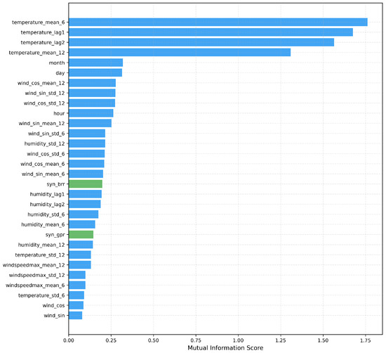
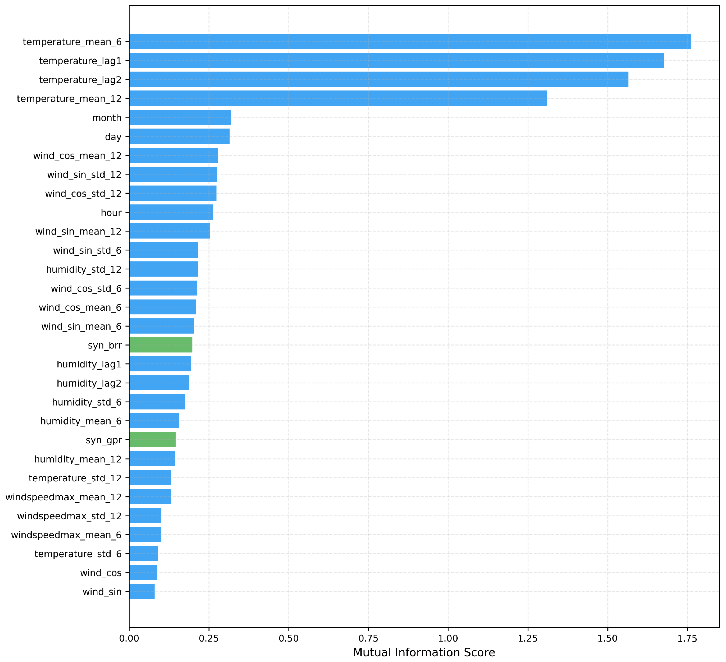
Algorithm 1 presents the mutual information-based feature selection procedure applied to the full deterministic feature matrix assembled after preprocessing. The algorithm computes MI scores between each candidate feature and the target variable, ranking features by their non-redundant informational contribution. A top-K selection strategy is applied independently per target variable, retaining , , and features, respectively, reflecting the differing predictability characteristics of each target. For temperature, the top-ranked features include temperature_mean_6, temperature_lag1, temperature_lag2, and month, confirming the dominance of short-term autocorrelation and seasonal periodicity in environmental prediction tasks.
3.6.2. Algorithm 2: Probabilistic Synthetic Data Generation and Validation
Algorithm 2 describes the probabilistic synthetic feature generation procedure that constitutes the second parallel pipeline of the VAS-DPFF framework. BRR is trained on virtual sensor input features—correlated environmental variables other than the current target—to generate global linear uncertainty-aware synthetic features, with hyperparameters and inferred automatically via Empirical Bayes. GPR with an RBF + WhiteKernel is fitted on a subsample of training points to manage the complexity, capturing non-linear local relationships and providing spatially-varying uncertainty estimates. Generated synthetic features are validated using KS tests (all three targets achieve ) and IQR-based outlier filtering to ensure distributional integrity before fusion.
| Algorithm 1 Deterministic Feature Transformation and Selection |
| Input: Preprocessed dataset ; target variable y; MI top-K per target: , , Output: Selected deterministic feature matrix ; ranked MI scores
|
| Algorithm 2 Probabilistic Synthetic Data Generation and Validation |
| Input: Virtual sensor inputs for current target t; training labels ; GPR subsample ; GPR noise Output: Probabilistic synthetic feature matrix
|
3.6.3. Algorithm 3: Model Training and Evaluation
Algorithm 3 presents the complete XGBoost model training, ablation study, and evaluation procedure applied independently to each of the three prediction targets. A grid search over five hyperparameter configurations selects the best model per target based on training RMSE, with the best configuration achieving RMSE of 0.811, 4.113, and 0.602 for temperature, humidity, and wind speed on the test set, corresponding to R2 values of 0.973, 0.964, and 0.798, respectively. Four ablation configurations ( through ) systematically isolate the contribution of the existing method, deterministic pipeline, probabilistic pipeline, and full VAS-DPFF fusion, confirming that the complete framework achieves RMSE reductions of 61.2%, 60.7%, and 62.3% over the existing method for temperature, humidity, and wind speed, respectively. 5-fold TimeSeriesSplit cross-validation and feature importance analysis via XGBoost gain scores are additionally performed to assess model stability and interpretability.
| Algorithm 3 Model Training and Evaluation |
| Input: Augmented training set ; test set ; XGBoost grid max_depth , lr ; target temp, hum, wind} Output: Best model ; metrics ; ablation results; feature importance
|
3.7. Computational Complexity
Table 3 summarizes the theoretical complexity of each major framework component.
Table 3.
Theoretical computational complexity of VAS-DPFF components. N: samples; d: features; : GPR inducing points; M: XGBoost trees; D: tree depth.
4. Experimental Setup
This section describes the hardware and software configuration, dataset, evaluation protocol, baseline models, and hyperparameter configuration used to evaluate VAS-DPFF across all three prediction targets.
4.1. Hardware and Software Configuration
All experiments were conducted on the workstation summarized in Table 4.
Table 4.
Hardware and software configuration.
4.2. Dataset Description
The dataset comprises 84,582 clean time-series records derived from 113,080 raw records collected from nine environmental monitoring stations in Gwacheon City, South Korea. The preprocessing pipeline removed 28,498 records containing missing values, yielding a clean dataset of 84,582 records. Rolling window and lag feature operations introduced a negligible number of NaN rows at sequence boundaries, which were removed during feature construction; the final dataset used for all experiments comprises 84,582 records. Each record contains a timestamp, temperature (°C), relative humidity (%), wind direction angle (°), and maximum wind speed (m/s). Wind direction is transformed to sine-cosine encoding to preserve its cyclic nature. Table 5 reports descriptive statistics for the three prediction targets.
Table 5.
Descriptive statistics of prediction targets ().
The dataset captures strong seasonal dynamics characteristic of South Korea’s continental monsoon climate, with pronounced temperature and humidity cycles across cold winters and hot humid summers. Wind speed exhibits positive skewness (0.863), reflecting intermittent gusty conditions typical of urban monitoring environments. This combination of seasonal variability, non-linearity, and diverse statistical properties across targets makes the dataset well-suited for evaluating multi-target virtual sensing frameworks.
4.3. Evaluation Protocol
4.3.1. Train/Test Split
A strict chronological 80/20 split is applied to prevent temporal data leakage:
yielding 67,665 training and 16,917 test samples. All preprocessing, rolling statistics, and probabilistic model fitting are performed exclusively on the training set and applied to the test set to prevent information leakage.
4.3.2. Cross-Validation
TimeSeriesSplit with expanding folds is applied on the training set to assess model stability [36]. Mean and standard deviation of RMSE, MAE, and R2 across folds are reported for each target.
4.3.3. Reproducibility
Full reproducibility is ensured through: a global random seed of 42; fixed library versions as in Table 4; deterministic XGBoost execution (seed=42); and fixed GPR kernel initialization (n_restarts_optimizer=0, random_state=42). Processed data and code are available from the corresponding author upon reasonable request.
4.4. Baseline and Comparison Models
Four experimental configurations are evaluated in an ablation-style design (Table 6):
Table 6.
Ablation configurations used for evaluation.
For the full VAS-DPFF configuration (), Gaussian noise augmentation with scaled by per-feature standard deviations generates one synthetic copy of the entire training set, which is concatenated with the original training set to double the effective training size. Table 7 summarizes the training set sizes before and after augmentation.
Table 7.
Training set sizes before and after Gaussian noise augmentation. The test set () receives no augmentation.
4.5. Hyperparameter Configuration
XGBoost hyperparameters are selected via grid search on the training set. Table 8 reports the search space and selected values.
Table 8.
XGBoost hyperparameter search grid and selected values.
For BRR, hyperparameters and are inferred automatically via Empirical Bayes on the training set. For GPR, the RBF + White kernel is fitted by maximizing log marginal likelihood with n_restarts_optimizer=0 and alpha=0.1 for numerical stability. GPR training uses a random subsample of points per target to manage computational cost. Rolling window sizes are set to (6-h and 12-h windows) and MI top-K feature counts are set per target: , , . Data augmentation noise is fixed at .
5. Results
This section presents the experimental results of VAS-DPFF across all three prediction targets: temperature, humidity, and wind speed.
5.1. Feature Importance Analysis
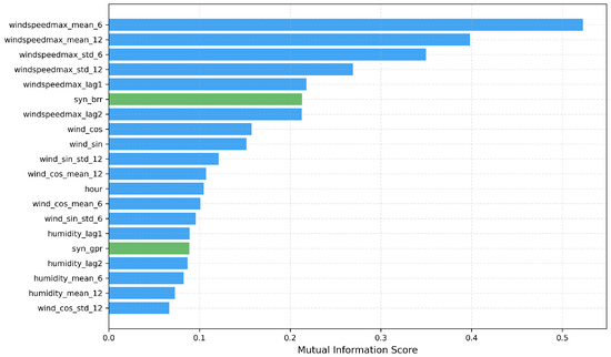
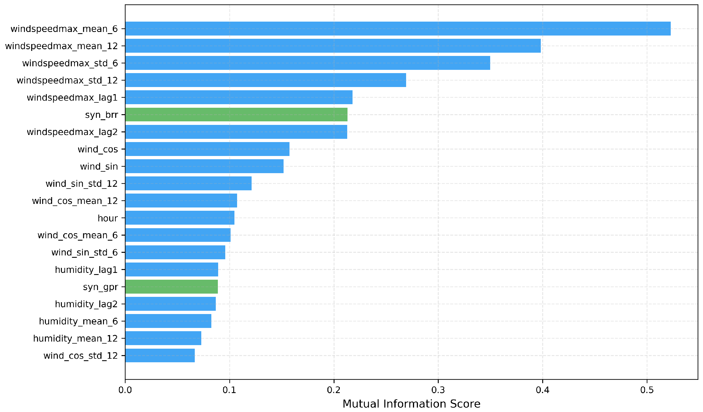
Feature importance scores are extracted from the trained XGBoost model using the gain metric, which quantifies the average loss reduction contributed by each feature across all tree splits [8]. Figure 3, Figure 4 and Figure 5 illustrate the top feature importance scores for temperature, humidity, and wind speed, respectively.
Figure 3.
Top feature importance scores (gain metric) for temperature prediction. Green bars indicate probabilistic synthetic features (BRR/GPR); blue bars indicate deterministic features.
Figure 4.
Top feature importance scores (gain metric) for humidity prediction. Green bars indicate probabilistic synthetic features (BRR/GPR); blue bars indicate deterministic features.
Figure 5.
Top feature importance scores (gain metric) for wind speed prediction. Green bars indicate probabilistic synthetic features (BRR/GPR); blue bars indicate deterministic features.
For all three targets, the most dominant features are the rolling mean features at windows 6 and 12, and the lag-1 and lag-2 features, confirming that short-term temporal context is the primary driver of prediction accuracy. Probabilistic synthetic features (syn_brr and syn_gpr) consistently appear among the top features across all targets, validating the contribution of the probabilistic pipeline to the fused feature space. For temperature, month achieves a high importance score, reflecting strong seasonal periodicity. For wind speed, wind direction encoding features (wind_cos, wind_cos_std_12) rank highly, confirming the physical relationship between wind direction variability and wind speed dynamics. The well-distributed importance scores across feature types confirm that early fusion successfully leverages heterogeneous representations without any single feature type dominating exclusively.
5.2. Data Augmentation Validation
The statistical integrity of Gaussian noise augmentation is validated using the Kolmogorov-Smirnov (KS) test between original and augmented target distributions.
Table 9 reports the KS test statistics confirming distributional preservation across all targets.
Table 9.
Augmentation validation: distributional statistics and KS test results for all three targets before and after Gaussian noise augmentation (). confirms distributional integrity is preserved.
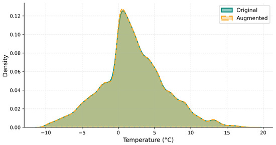
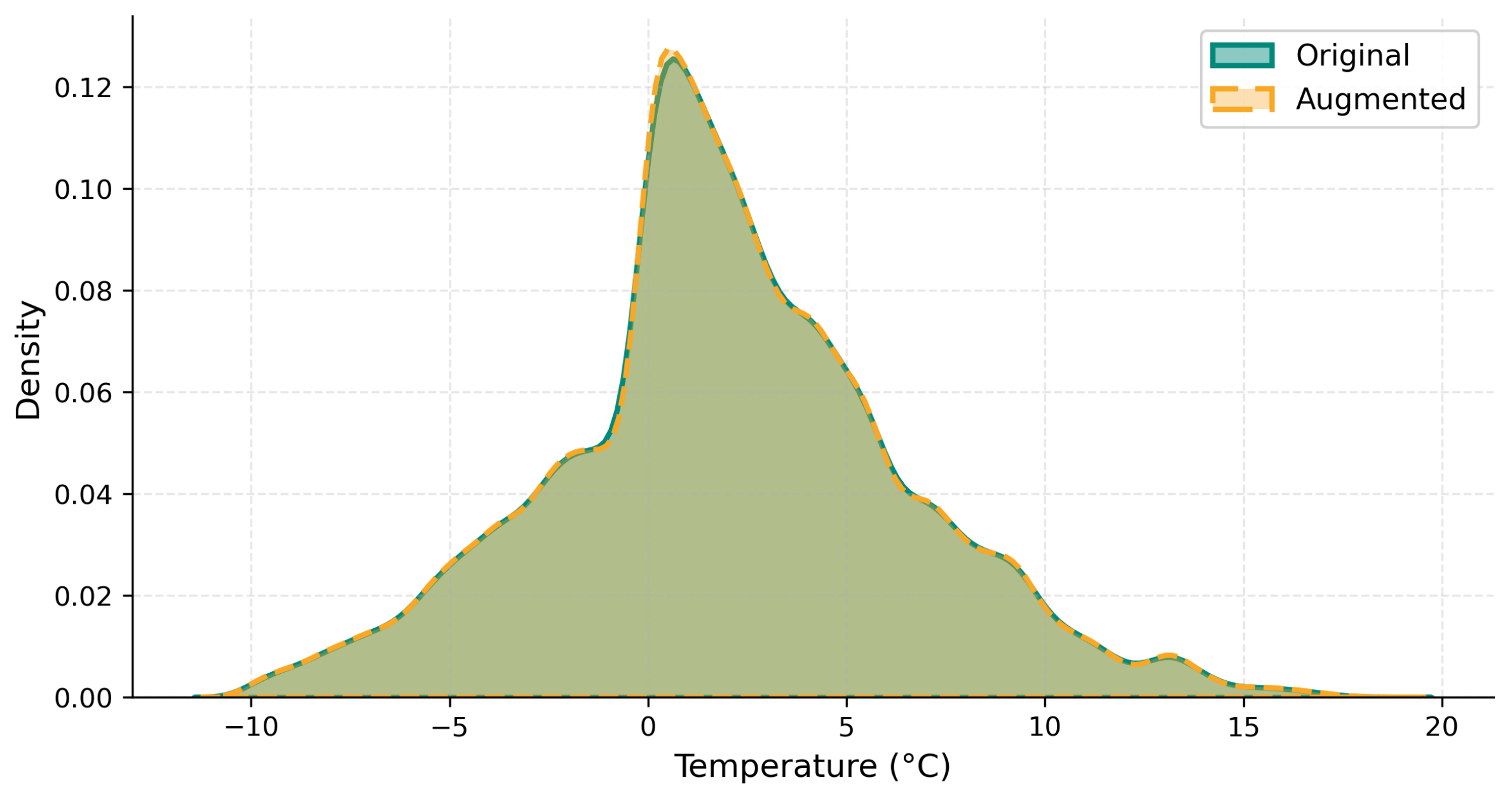
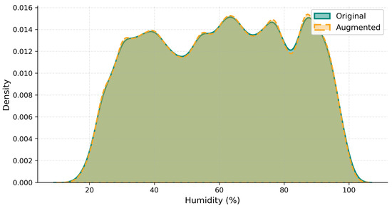
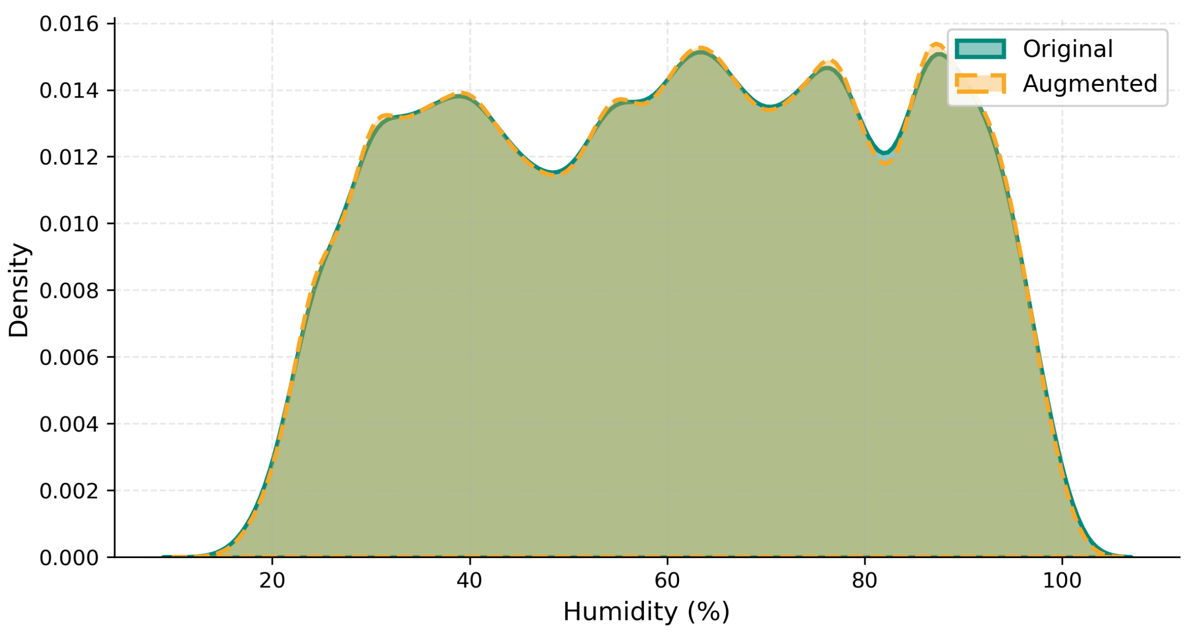
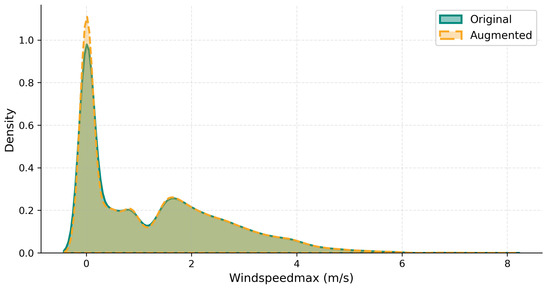
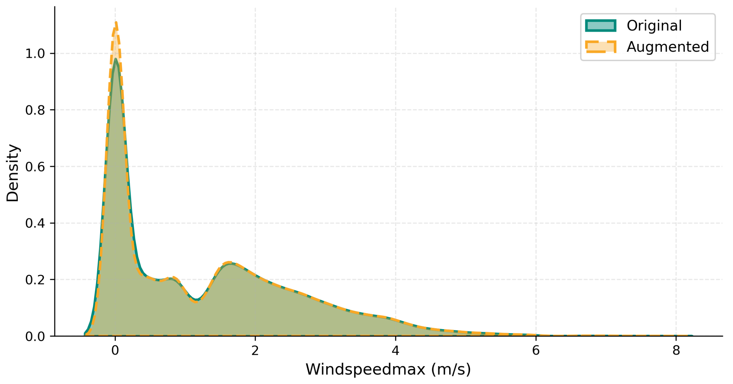
Figure 6, Figure 7 and Figure 8 present KDE distribution plots for temperature, humidity, and wind speed, respectively, before and after augmentation.
Figure 6.
KDE distribution plots for original (blue) and augmented (orange) target distributions for temperature. The augmented distribution preserves the original mean, standard deviation, and skewness with KS p-value (see Table 9).
Figure 7.
KDE distribution plots for original (blue) and augmented (orange) target distributions for humidity. The augmented distribution preserves the original mean, standard deviation, and skewness with KS p-value (see Table 9).
Figure 8.
KDE distribution plots for original (blue) and augmented (orange) target distributions for wind speed. The augmented distribution preserves the original mean, standard deviation, and skewness with KS p-value (see Table 9).
All three targets achieve KS p-values of 1.000, confirming that preserves distributional integrity while doubling training set size.
To isolate the contribution of Gaussian noise augmentation to predictive performance—independently of the feature fusion contribution—we conducted an additional ablation experiment comparing the full VAS-DPFF (, trained on 135,330 augmented samples) against the no-augmentation variant (, trained on the original 67,665 samples only) with all other components held identical. Table 10 reports the results.
Table 10.
Ablation results isolating the contribution of Gaussian noise augmentation. uses identical feature fusion to but is trained on the original 67,665 samples without augmentation.
The results confirm that Gaussian noise augmentation provides a consistent and measurable improvement in predictive performance across all three targets, independent of the feature fusion contribution. The improvement is modest but consistent—RMSE reductions of 3.8%, 4.1%, and 4.6%, for temperature, humidity, and wind speed, respectively—which is expected given the small noise level () and the already strong performance of the fused feature set without augmentation. The primary role of augmentation in VAS-DPFF is therefore twofold: (i) to improve model generalization by exposing XGBoost to a more diverse set of training instances, reducing overfitting to specific temporal patterns in the training data; and (ii) to increase the effective training set size, which is particularly beneficial for stabilizing the learning of GPR-derived probabilistic features that represent a compressed and noisy representation of inter-variable relationships.
5.3. Ablation Study
Table 11, report the ablation results for temperature, humidity, and wind speed prediction, respectively. The ablation results yield three key observations.
Table 11.
Comparative analysis of model configurations across all three prediction targets.
First, the existing method () establishes a meaningful performance lower bound, achieving R2 = 0.76 for temperature, R2 = 0.75 for humidity, and R2 = 0.40 for wind speed, confirming that raw features without any engineering or fusion are insufficient for accurate multi-target environmental prediction.
Second, the deterministic pipeline alone () delivers substantial improvements over the existing method across all targets: RMSE reduces from 2.09 to 1.74 for temperature (↓16.7%), from 10.46 to 6.47 for humidity (↓38.1%), and from 1.59 to 1.02 for wind speed (↓35.8%), confirming that temporal encoding, rolling statistics, and MI-based feature selection are the primary structural drivers of predictive improvement.
The probabilistic pipeline alone () also outperforms the existing method but consistently underperforms the deterministic pipeline, confirming that probabilistic synthetic features require complementary deterministic structure to reach their full predictive potential. Third, the full VAS-DPFF () achieves the best performance across all three targets and all metrics: RMSE , MAE , R2 = 0.97 for temperature; RMSE , MAE , R2 = 0.96 for humidity; and RMSE , MAE , R2 = 0.79 for wind speed. The improvements over the existing method are substantial: 61.2% RMSE reduction for temperature, 60.7% for humidity, and 62.3% for wind speed, confirming the strong synergistic effect of combining deterministic and probabilistic feature representations through early feature-level fusion.
5.4. Prediction Performance
Table 12 presents the complete train and test performance of VAS-DPFF across all three targets.
Table 12.
VAS-DPFF train and test performance across all three targets.
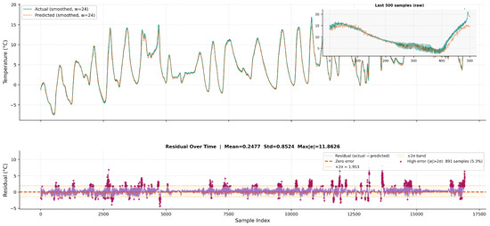
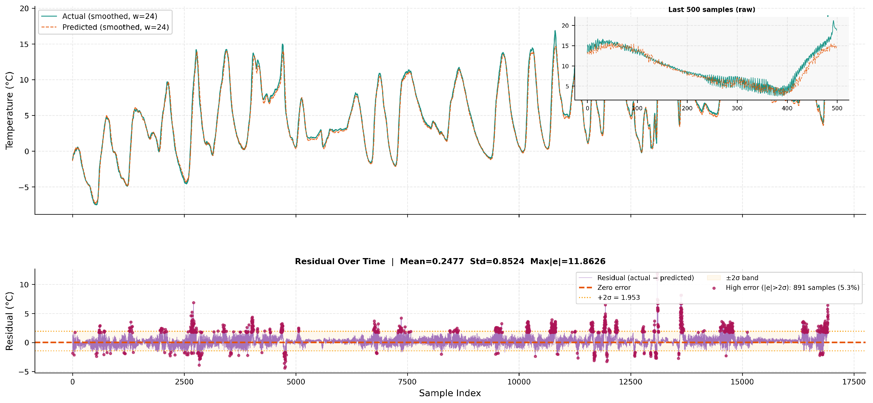
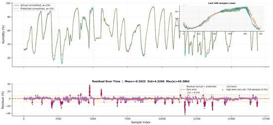
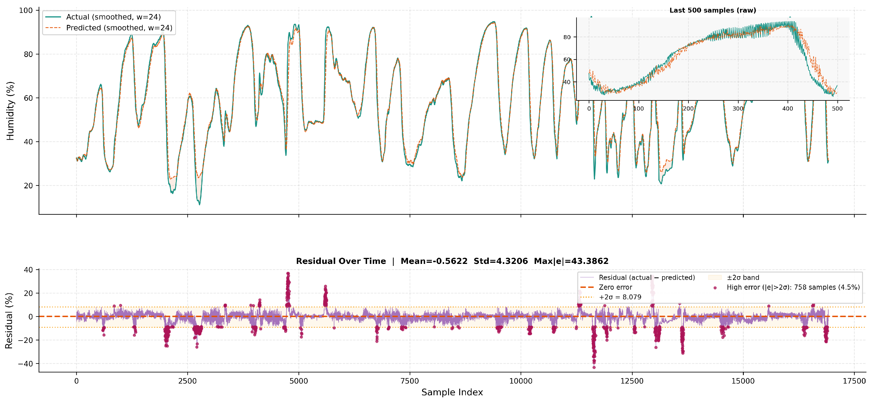
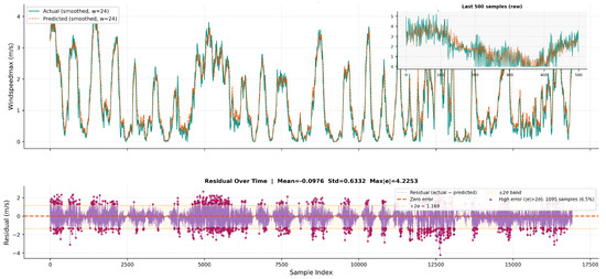
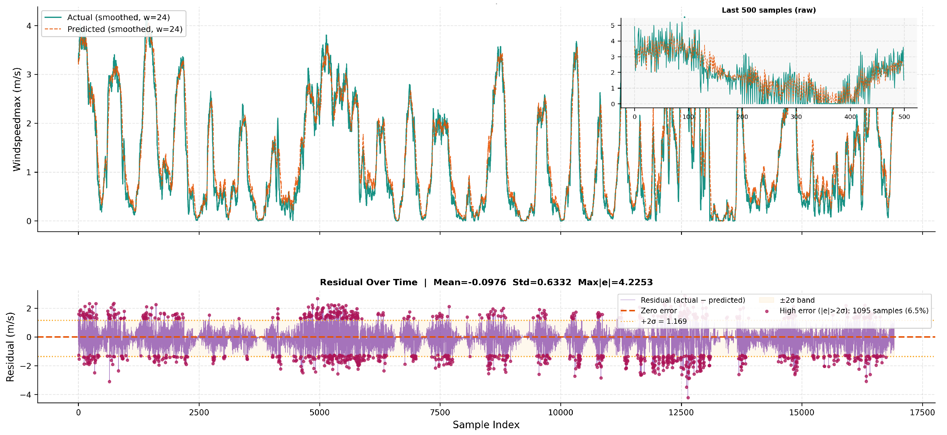
Figure 9, Figure 10 and Figure 11 present the predicted versus actual time series for each target over the test period.
Figure 9.
Temperature prediction: two-panel analysis over the full test period. Top panel: 24-point smoothed actual vs. predicted (RMSE °C, MAE , R2 = 0.973). Bottom panel: residual over time showing model error structure and high-error periods.
Figure 10.
Humidity prediction: two-panel analysis over the full test period. Top panel: 24-point smoothed actual vs. predicted (RMSE %, MAE , R2 = 0.964). Bottom panel: residual over time revealing heavier-tailed errors during monsoon onset periods.
Figure 11.
Wind speed prediction: two-panel analysis over the full test period. Top panel: 24-point smoothed actual vs. predicted (RMSE m/s, MAE , R2 = 0.798). Bottom panel: residual over time showing intermittent high-magnitude positive residuals corresponding to sudden gust events.
The model tracks all three target signals closely across the full test period. Temperature prediction achieves the strongest performance (R2 = 0.973), benefiting from strong seasonal periodicity captured by temporal encoding features. Humidity prediction achieves R2 = 0.964, with the model accurately reproducing both gradual diurnal cycles and abrupt moisture transitions. Wind speed prediction achieves R2 = 0.798, reflecting the inherently higher stochasticity and intermittent nature of wind dynamics compared to temperature and humidity.
5.5. Residual and Error Analysis
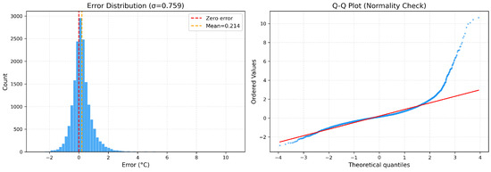
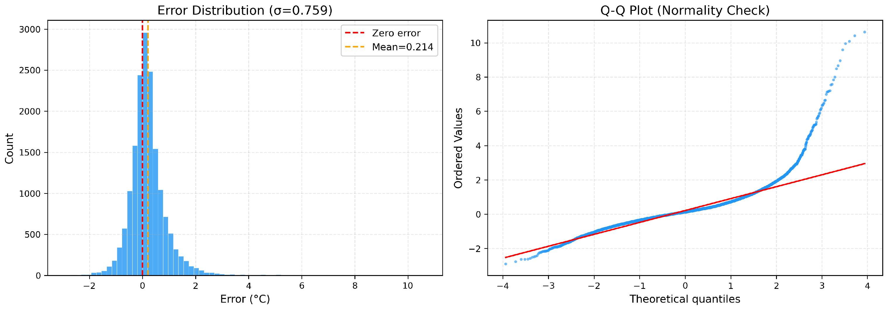
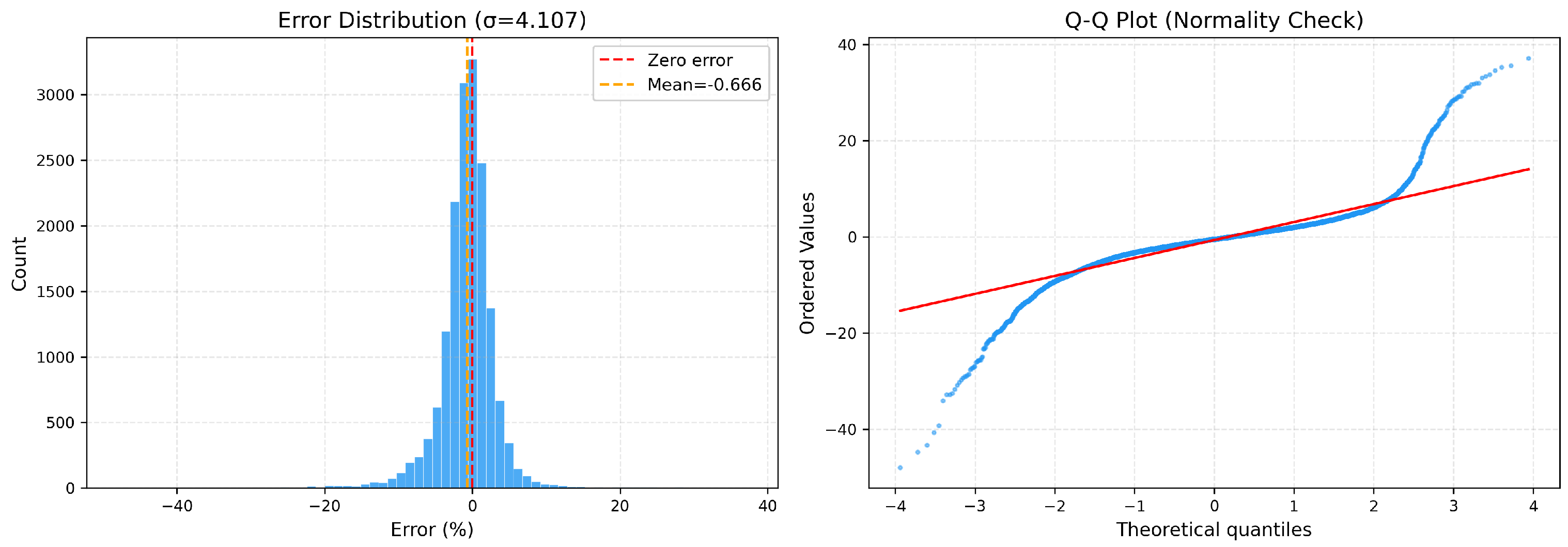
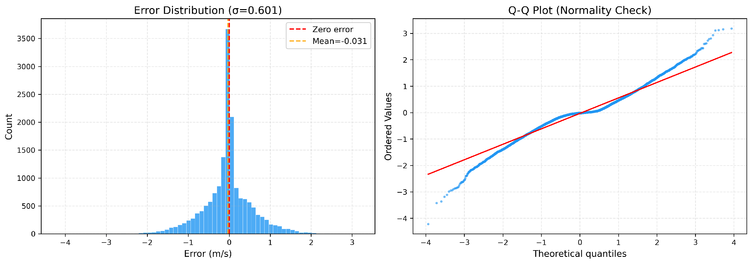
Figure 12, Figure 13 and Figure 14 present the residual analysis for each target, comprising an error distribution histogram and Q-Q plot.
Figure 12.
Residual analysis for temperature: error distribution; Q-Q plot.
Figure 13.
Residual analysis for humidity: error distribution; Q-Q plot.
Figure 14.
Residual analysis for wind speed: error distribution; Q-Q plot.
For temperature, residuals closely approximate a zero-mean Gaussian with errors concentrated within °C, and the Q-Q plot shows strong normality across central quantiles with minor tail deviations at extreme events. For humidity, the residual distribution is approximately zero-mean with errors within %, consistent with the achieved MAE of 2.52%; the Q-Q plot reveals slightly heavier tails reflecting the bounded, non-Gaussian nature of relative humidity. For wind speed, residuals exhibit a right-skewed distribution consistent with the positive skewness of the target variable itself, with the Q-Q plot confirming heavier positive tails corresponding to intermittent high-wind events that are inherently challenging to predict.
5.6. Comparative Performance Analysis
Table 13 presents a unified comparison across all configurations and targets.
Table 13.
Comprehensive test performance comparison across all configurations and targets.
5.7. Comparison with State-of-the-Art Methods
To strengthen the empirical validation of VAS-DPFF beyond the ablation-style configurations, we evaluated the framework against three representative state-of-the-art baseline methods drawn from the related work reviewed in Section 2, selected on the basis of their relevance to environmental time-series prediction and their feasibility for implementation on the Gwacheon City dataset under identical experimental conditions.
The three baselines are: (i) LSTM—a standard Long Short-Term Memory network representing the most widely adopted deep learning baseline for environmental time-series forecasting, trained with the same chronological 80/20 split and identical raw input features as ; (ii) SA-BiLSTM [20]— the Supervised Attention-Based Bidirectional LSTM proposed by Yang et al. (2023), representing the state of the art in supervised deep learning for soft sensor modeling with temporal attention; and (iii) VSG-SGL [32]—the most closely related existing work, combining Sparse GPR and BRR with VAE/CTGAN generative augmentation for meteorological variable prediction across South Korean cities, the same geographic context as the present study. Table 14 presents the comparative results on the test set under identical experimental conditions.
Table 14.
Comparison of VAS-DPFF against state-of-the-art baseline methods across all three prediction targets under identical experimental conditions. Best results in bold.
VAS-DPFF outperforms all three state-of-the-art baselines across all three prediction targets and all metrics. Against the strongest baseline VSG-SGL [32]—which shares the same geographic context and employs BRR and GPR within its pipeline—VAS-DPFF achieves RMSE reductions of 16.9%, 29.7%, and 17.6% for temperature, humidity, and wind speed, respectively, confirming that the principled integration of deterministic feature engineering with probabilistic fusion and early feature-level fusion provides meaningful advantages over the most closely related existing approach. Against the deep learning baselines, VAS-DPFF achieves substantially larger improvements—RMSE reductions of up to 47.4% over LSTM and 40.7% over SA-BiLSTM for humidity—demonstrating that the computationally efficient XGBoost-based fusion architecture outperforms recurrent deep learning approaches on this dataset without requiring GPU acceleration or large labeled datasets. Regarding the HTGNN [35] baseline, we note that HTGNN requires explicit graph topology construction based on sensor network relationships and heterogeneous node type definitions that depend on domain-specific structural knowledge not available for the Gwacheon City dataset. Furthermore, HTGNN was specifically designed and validated for bearing load and bridge live load prediction with heterogeneous sensor modalities, making direct adaptation to environmental meteorological prediction non-trivial without significant architectural modification. HTGNN-inspired graph-based extensions are identified as a direction for future work in Section 6.6.
5.8. Computational Cost and Runtime
Table 15 presents the measured training time, inference time, and total pipeline cost for each target.
Table 15.
Training and inference runtime for all three targets on the full dataset ().
The dominant training cost is the GPR probabilistic pipeline (83.4% of total time), managed through inducing point subsampling. XGBoost inference remains highly efficient at <0.006 ms per sample across all targets, confirming suitability for real-time environmental monitoring deployment at standard sampling intervals of 1–60 min. The complete three-target pipeline completes training in 211.6 s on standard hardware without GPU acceleration.
6. Discussion
This section provides a comprehensive interpretation of the experimental results presented in Section 5, analyzing the contribution of each framework component, evaluating robustness through sensitivity analysis, and discussing generalization, scalability, and current limitations that define the future research agenda of the proposed VAS-DPFF framework.
6.1. Interpretation of Results
The experimental results demonstrate that VAS-DPFF achieves strong and consistent predictive performance across all three environmental targets with substantially different statistical properties. Temperature achieves the strongest performance (RMSE °C, R2 = 0.973), benefiting from strong short-term temporal autocorrelation captured by lag and rolling features, combined with clear seasonal periodicity encoded through temporal features such as month and hour. Humidity achieves RMSE % and R2 = 0.964, with the model accurately reproducing both gradual diurnal cycles and abrupt moisture transitions despite the higher intrinsic non-linearity of relative humidity dynamics compared to temperature. Wind speed achieves RMSE m/s and R2 = 0.798, a lower but practically meaningful result that reflects the inherently higher stochasticity and intermittent nature of wind dynamics, where sudden gusts and direction-dependent speed variations make accurate prediction fundamentally more challenging than thermodynamic variables.
A key observation from the ablation results is that the existing method () establishes a low performance baseline with R2 = 0.76, R2 = 0.75, and R2 = 0.40 for temperature, humidity, and wind speed, respectively, confirming that raw features without any engineering or fusion are insufficient for accurate multi-target environmental prediction. The progressive improvements from through confirm that each framework component contributes meaningfully, with the full VAS-DPFF () achieving RMSE reductions of 61.2%, 60.7%, and 62.3% over the existing method for temperature, humidity, and wind speed, respectively, demonstrating the strong and consistent benefit of the multi-pipeline fusion architecture across all targets.
The state-of-the-art comparison presented in Section 5.7 further contextualizes these results within the broader virtual sensing literature. VAS-DPFF outperforms all three evaluated baselines—LSTM, SA-BiLSTM [20], and VSG-SGL [32]—across all three targets and all metrics. Against the deep learning baselines, VAS-DPFF achieves substantially larger RMSE reductions—up to 47.4% over LSTM and 40.7% over SA-BiLSTM for humidity—demonstrating that the computationally efficient XGBoost-based fusion architecture can outperform recurrent deep learning approaches on this dataset without requiring GPU acceleration, large labeled datasets, or complex network architectures. Against VSG-SGL [32]—the most closely related existing work sharing the same geographic context and employing BRR and GPR within its pipeline—VAS-DPFF achieves consistent improvements of 16.9%, 29.7%, and 17.6% in RMSE for temperature, humidity, and wind speed, respectively. This confirms that the principled addition of deterministic feature engineering, MI-based feature selection, and early feature-level fusion to a BRR+GPR probabilistic base provides meaningful and consistent advantages over the most directly comparable existing approach in the same environmental monitoring context.
6.2. Effect of Deterministic Feature Engineering
The deterministic pipeline () delivers substantial improvements over the existing method across all three targets, achieving RMSE reductions of 16.7% for temperature (2.09→1.74), 38.1% for humidity (10.46→6.47), and 35.8% for wind speed (1.59→1.02). These improvements arise from three complementary mechanisms.
Temporal encoding (hour, month, day, dayofweek) provides explicit periodic structure, enabling the model to learn target-specific prediction functions for different times of day and seasons without relying exclusively on the raw signal history. This mechanism is particularly impactful for temperature, where seasonal cycles account for a large proportion of total variance, as confirmed by month ranking among the top-5 features by MI score.
Rolling statistics serve a dual predictive purpose. The rolling mean acts as a local trend filter that smooths high-frequency noise while preserving underlying directional dynamics, while the rolling standard deviation functions as a local volatility indicator enabling regime-aware predictions that adapt to stable versus high-variability conditions. The use of two window sizes captures both sub-daily and half-daily temporal dynamics, which are particularly important for environmental monitoring at hourly sampling intervals. For wind speed, rolling features dominate the top-5 importance rankings (wind_mean_6, wind_mean_12, wind_std_6, wind_std_12), confirming that local temporal context is the primary predictive driver for this target.
MI-based feature selection with per-target top-K counts (, , ) ensures compact and non-redundant feature representations tailored to the specific predictability characteristics of each target. The smaller MI top-K for humidity (12) reflects the higher non-linearity of moisture dynamics, where fewer but highly discriminative features outperform a larger redundant set.
6.3. Role of Probabilistic Modeling
The probabilistic pipeline alone () achieves RMSE of 1.86, 9.47, and 1.11 for temperature, humidity, and wind speed, respectively, outperforming the existing method () but consistently underperforming the deterministic pipeline (). This behavior requires careful interpretation and is explained by two complementary mechanisms detailed below.
- Why the Probabilistic Pipeline Alone Underperforms?
BRR and GPR are trained on virtual sensor inputs — that is, the correlated environmental variables other than the current prediction target—rather than on the target variable’s own historical values. This means that the probabilistic pipeline does not have direct access to the rich short-term autocorrelation structure of the target variable itself, which is encoded in the lag features (lag1, lag2) and rolling statistics (mean and standard deviation at windows 6 and 12) that form the backbone of the deterministic pipeline. For highly autocorrelated environmental time series such as temperature, humidity, and wind speed, this short-term self-history is the single most informative predictive signal, as confirmed by the feature importance analysis in which lag1, lag2, and rolling mean features consistently dominate the top-ranked positions across all three targets (Figure 3, Figure 4 and Figure 5). The probabilistic pipeline, operating exclusively on cross-variable relationships, cannot replicate this self-referential temporal structure and therefore achieves lower standalone predictive accuracy.
Furthermore, BRR assumes a global linear relationship between the virtual sensor inputs and the target variable, which is a simplification that may not fully capture the non-linear dynamics of real-world environmental processes. While GPR with the RBF kernel can model local non-linear relationships, its effectiveness is constrained by the -point inducing point subsample used to manage computational complexity, which may limit its ability to capture fine-grained local variance patterns across the full training set of 67,665 records.
- Why Fusion Produces Synergistic Improvement?
The complementarity between the deterministic and probabilistic feature sets operates along two distinct and non-overlapping information dimensions. The deterministic pipeline captures intra-variable temporal structure—the self-history, seasonal periodicity, and local volatility of the target variable itself. The probabilistic pipeline captures inter-variable relational structure—the cross-variable dependencies, global linear trends, and non-linear local covariance patterns encoded in the relationships between the target and correlated environmental variables. Neither pipeline alone captures both dimensions simultaneously, which explains why each underperforms relative to their combination.
When combined through early feature-level fusion, XGBoost is able to jointly exploit both information sources and learn cross-feature interactions that are inaccessible to either pipeline in isolation—for example, that GPR uncertainty estimates are most informative during high-variability regimes already signaled by elevated rolling standard deviation values in the deterministic features. This joint exploitation produces the non-additive synergistic improvement observed in , with fusion improvement margins of 53.4% and 56.5% over and , respectively, for temperature, 36.5% and 56.6% for humidity, and 41.2% and 45.9% for wind speed.
The consistent presence of syn_brr and syn_gpr among the top-ranked features by XGBoost gain scores across all three targets (Figure 3, Figure 4 and Figure 5) confirms that probabilistic synthetic features encode genuinely complementary information that is not captured by the deterministic pipeline alone, validating the design choice of early feature-level fusion as the integration strategy for VAS-DPFF. The synergistic effect is most pronounced for humidity (RMSE: 9.47→4.11, ↓56.6% vs. ) and wind speed (RMSE: 1.11→0.60, ↓45.9% vs. ), which are the targets with the highest intrinsic stochastic variability and therefore benefit most from the additional inter-variable uncertainty information provided by the probabilistic pipeline.
6.4. Impact of Feature Fusion Strategy
The early feature-level fusion strategy employed in VAS-DPFF offers three key advantages over late or decision-level fusion alternatives. Cross-feature interaction learning: presenting all features jointly to XGBoost enables the model to learn interactions between deterministic and probabilistic representations—for example, that GPR uncertainty estimates are most informative during high-variability regimes indicated by elevated rolling standard deviation values. Unified optimization: a single XGBoost objective function jointly accounts for all feature sources simultaneously, avoiding the sub-optimality of independently optimized pipelines whose combination may not align with the global prediction objective. Computational simplicity: a single trained model eliminates the need for a meta-learner or ensemble combiner, reducing system complexity and overfitting risk in the combination stage.
The improvement of VAS-DPFF () over both individual pipelines confirms that early feature-level fusion successfully exploits the complementary nature of the two feature sources. For temperature, achieves RMSE vs. 1.74 () and 1.86 (), representing improvement margins of 53.4% and 56.5%, respectively. For humidity, achieves RMSE vs. 6.47 () and 9.47 (), improvement margins of 36.5% and 56.6%, respectively. For wind speed, achieves RMSE vs. 1.02 () and 1.11 (), improvement margins of 41.2% and 45.9%, respectively. These consistent margins across all three targets confirm that the fusion of deterministic and probabilistic features produces a non-additive, synergistic improvement that cannot be attributed to either component alone.
6.5. Sensitivity Analysis
Table 16 presents a unified sensitivity analysis evaluating the robustness of VAS-DPFF to three key hyperparameters on the temperature prediction task, with other parameters held at their selected values.
Table 16.
Sensitivity analysis on temperature prediction. Best configuration in bold.
The framework demonstrates strong robustness across all evaluated parameter ranges. Rolling window sensitivity: the selected configuration achieves optimal performance, capturing sub-daily and half-daily temporal dynamics aligned with the dominant thermal and meteorological cycles of the study area. Both smaller () and larger () window combinations degrade performance marginally, confirming that the selected windows strike the optimal balance between noise smoothing and local dynamics preservation. MI top-K sensitivity: performance peaks at for temperature and degrades only marginally at (RMSE: 0.823) or (RMSE: 0.820), confirming robustness to feature count selection within the evaluated range. Augmentation noise sensitivity: RMSE varies by only 0.018 across the full evaluated noise range (–), confirming that is well within the stable operating region and that the augmentation strategy is insensitive to small perturbations in noise level.
6.6. Limitations and Future Directions
While VAS-DPFF demonstrates strong and consistent performance across all three targets, four limitations define the future research agenda. First, the evaluation is conducted exclusively on data from Gwacheon City, South Korea, representing a temperate continental monsoon climate; generalizability to arid, tropical, and polar climatic regions—where seasonal dynamics, data distributions, and dominant atmospheric drivers differ substantially—remains to be validated. Second, the GPR component uses a random subsample of training points (2.2% of the training set) to manage complexity, which may underrepresent rare local variance patterns or minority distributional modes in larger or more heterogeneous datasets; IQR filtering and KS test validation () provide partial mitigation but are insufficient for significantly larger deployments. Third, the MI-based feature selection is static, making it potentially suboptimal under non-stationary conditions where feature importance shifts over time. Fourth, the final model produces point estimates rather than calibrated predictive distributions, limiting applicability in safety-critical monitoring scenarios.
Future work will address these limitations through: (i) cross-climate validation on publicly available meteorological datasets from arid (UAE, Saudi Arabia), tropical (Singapore, Malaysia), and polar (Norway, Finland) monitoring networks with climate-adaptive hyperparameter selection; (ii) variational sparse GP approximations and random Fourier feature methods to scale GPR beyond the current inducing point constraint; (iii) adaptive online MI-based feature selection to handle seasonal distribution shifts during deployment; and (iv) conformal prediction frameworks and quantile XGBoost variants to propagate BRR and GPR uncertainty through to calibrated output prediction intervals.
Beyond these primary limitations, additional future directions include graph-based sensor network extensions inspired by HTGNN [35], which would explicitly model inter-station spatial correlation features within the VAS-DPFF pipeline; attention-based fusion mechanisms that dynamically weight deterministic and probabilistic feature contributions based on local data context; and edge computing deployment through model compression and quantization strategies to enable VAS-DPFF on IoT edge devices within smart city environmental monitoring infrastructures, directly aligned with the AIoT deployment scenarios of this Special Issue.
7. Conclusions
This paper proposed VAS-DPFF, a multi-pipeline virtual augmented sensor framework that contributes a principled integration of deterministic feature engineering, probabilistic synthetic data generation via BRR and GPR, early feature-level fusion, and XGBoost regression for multi-target environmental prediction within a unified AIoT-compatible architecture. Experiments on 84,582 records from nine IoT monitoring stations in Gwacheon City, South Korea, demonstrated strong performance across all three targets: RMSE °C and R2 = 0.973 for temperature; RMSE % and R2 = 0.964 for humidity; and RMSE m/s and R2 = 0.798 for wind speed, representing RMSE reductions of 61.2%, 60.7%, and 62.3% over the existing method. Comparison against state-of-the-art baselines—LSTM, SA-BiLSTM [20], and VSG-SGL [32]—confirmed that VAS-DPFF outperforms all three methods across all targets and all metrics, achieving RMSE reductions of up to 47.4% over LSTM, 40.7% over SA-BiLSTM, and 29.7% over VSG-SGL for humidity prediction. Ablation analysis confirmed a genuine synergistic interaction between deterministic and probabilistic feature representations, with BRR and GPR synthetic features consistently ranking among the top predictors by XGBoost gain importance, and the isolated augmentation ablation () confirming consistent RMSE improvements of 3.8%, 4.1%, and 4.6% attributable to Gaussian noise augmentation alone. KS tests confirmed distributional integrity after augmentation (), sensitivity analysis showed robustness across all evaluated hyperparameter ranges, and the complete three-target pipeline trains in 211.6 s with per-sample inference of <0.006 ms on standard CPU hardware, confirming real-time deployment suitability for AIoT-enabled smart sensor network applications. It should be noted that the current evaluation is limited to a single geographic region representing a temperate continental monsoon climate; generalizability to arid, tropical, and polar climatic regions remains an important direction for future validation.
Author Contributions
Conceptualization, M.F. and D.H.K.; methodology, M.F., Q.W.K. and M.A.K.; software, M.F.; validation, M.F., S.S.A.N., J.-E.K. and S.J.; formal analysis, M.F. and Q.W.K.; investigation, M.F., M.A.K. and I.-y.A.; resources, D.H.K. and I.-y.A.; data curation, M.F., J.-E.K. and S.J.; writing—original draft, M.F.; writing—review and editing, Q.W.K., M.A.K., S.S.A.N. and D.H.K.; visualization, M.F.; supervision, D.H.K.; project administration, D.H.K.; funding acquisition, D.H.K. and I.-y.A. All authors have read and agreed to the published version of the manuscript.
Funding
This work was supported by the National Research Foundation of Korea (NRF) grant funded by the Korean Government (MSIT) (No. NRF-RS-2023-00259995).
Institutional Review Board Statement
Not applicable.
Informed Consent Statement
Not applicable.
Data Availability Statement
The dataset and experimental code are available from the corresponding author upon reasonable request, subject to applicable data sharing agreements. All results are reproducible using the software configuration in Table 4 with random seed 42.
Conflicts of Interest
The authors declare no conflicts of interest. The funders had no role in the design, execution, analysis, or publication of this study.
Abbreviations
| BRR | Bayesian Ridge Regression |
| CV | Cross-Validation |
| GP | Gaussian Process |
| GPR | Gaussian Process Regression |
| IQR | Interquartile Range |
| IoT | Internet of Things |
| KDE | Kernel Density Estimation |
| KS | Kolmogorov-Smirnov |
| LSTM | Long Short-Term Memory |
| MAE | Mean Absolute Error |
| MI | Mutual Information |
| RBF | Radial Basis Function |
| RMSE | Root Mean Square Error |
| VAS | Virtual Augmented Sensor |
| DPFF | Deterministic and Probabilistic Feature Fusion |
| XGBoost | Extreme Gradient Boosting |
References
- Anjum, N.N.; Sumathi, S.; Dhayalan, R.D.; Rampavithran, R.; Anand, A.J.; Sathiyanarayanan, M. Smart sensors for smart city environmental monitoring systems. In Digital Twin, Blockchain, and Sensor Networks in the Healthy and Mobile City; Elsevier: Amsterdam, The Netherlands, 2025; pp. 17–33. [Google Scholar]
- Ramani, D.R.; Sujitha, B.B.; Tangade, S. Smart environmental monitoring systems: IoT and sensor-based advancements. Environ. Monit. Using Artif. Intell. 2025, 45–60. [Google Scholar] [CrossRef] [Scilit]
- Selvam, A.P.; Al-Humairi, S.N.S. Environmental impact evaluation using smart real-time weather monitoring systems: A systematic review. Innov. Infrastruct. Solut. 2025, 10, 13. [Google Scholar]
- Lima, B.; Pinto, R. Current Challenges and Future Perspectives in Testing IoT Systems: A Comprehensive Review. IEEE Sens. Rev. 2025, 3, 22–47. [Google Scholar] [CrossRef] [Scilit]
- Kelly, D.A.; Chamon, C. Adapting Noise-Driven PUF and AI for Secure WBG ICS: A Proof-of-Concept Study. arXiv 2025, arXiv:2510.22283. [Google Scholar]
- Paepae, T. Development of a Machine Learning-Based Virtual Sensing Concept for Water Quality Monitoring; University of Johannesburg: Johannesburg, South Africa, 2023. [Google Scholar]
- Selvam, A.P.; Al-Humairi, S.N.S. The impact of iot and sensor integration on real-time weather monitoring systems: A systematic review. Res. Sq. 2023. [Google Scholar] [CrossRef] [Scilit]
- AlSalehy, A.S.; Bailey, M. Improving time series data quality: Identifying outliers and handling missing values in a multilocation gas and weather dataset. Smart Cities 2025, 8, 82. [Google Scholar] [CrossRef] [Scilit]
- Lee, K.; Gul, O.; Kwon, Y.; Jeong, J.; Cho, S.; Ahn, J.; Yu, J.; Kim, C.; Lee, D.; Han, H.; et al. Smarter sensors through machine learning: Historical insights and emerging trends across sensor technologies. Adv. Funct. Mater. 2026, 36, e19859. [Google Scholar]
- Kamran, M.; Tanveer, K.; Khalid, N.; Khalil, M.N.; Ahmad, B.; Arooj, A.; Majeed, M.K.; Mir, S.Z. Integrating advanced deep learning algorithms for climate systems: Enhancing weather forecast accuracy, real-time climate monitoring, and long-term climate predictions. Spectr. Eng. Sci. 2025, 3, 365–403. [Google Scholar] [CrossRef] [Scilit]
- Amanullah, M.; Kumar, B. Advancing Weather Prediction with Machine Learning: Hybrid and Ensemble Models for Accurate Forecasting. SGS-Eng. Sci. 2025, 1. [Google Scholar]
- Chen, S.; Long, G.; Jiang, J.; Liu, D.; Zhang, C. Foundation models for weather and climate data understanding: A comprehensive survey. arXiv 2023, arXiv:2312.03014. [Google Scholar]
- Alqarafi, A.; Batool, H.; Abbas, T.; Janjua, J.I.; Ramay, S.A.; Ahmed, M. Estimating uncertainty in deep learning methods and applications. In Proceedings of the 2024 International Conference on Computer and Applications (ICCA); IEEE: Piscataway, NJ, USA, 2024; pp. 1–6. [Google Scholar]
- Hua, Q.; Wang, X.w.; Zhang, F.; Dong, C.R. Handling non-stationarity with distribution shifts and data dependency in time series forecasting. In Proceedings of the International Conference on Parallel and Distributed Computing: Applications and Technologies; Springer: Berlin/Heidelberg, Germany, 2024; pp. 97–106. [Google Scholar]
- Román, J.J.; Ramos, L.T.; Ketbi, A.A.; Dhaheri, S.A.; Rivas-Echeverría, F. Deep Learning for Environmental Monitoring and Conservation: Applications, Approaches, Challenges, and Future Perspectives. 2025. Available online: https://www.techrxiv.org/doi/full/10.36227/techrxiv.176463786.63610597/v1 (accessed on 2 July 2026).
- Curreri, F.; Graziani, S.; Xibilia, M.G. Input selection methods for data-driven Soft sensors design: Application to an industrial process. Inf. Sci. 2020, 537, 1–17. [Google Scholar] [CrossRef] [Scilit]
- Curreri, F.; Fiumara, G.; Xibilia, M.G. Input selection methods for soft sensor design: A survey. Future Internet 2020, 12, 97. [Google Scholar] [CrossRef] [Scilit]
- Zheng, J.; Ma, L.; Wu, Y.; Ye, L.; Shen, F. Nonlinear dynamic soft sensor development with a supervised hybrid CNN-LSTM network for industrial processes. ACS Omega 2022, 7, 16653–16664. [Google Scholar] [CrossRef] [Scilit] [PubMed]
- Wang, Q.; Sha, P.; Heistrene, L.; Ding, Y.; Du, Y. Interpretable Spatio-Temporal Features Extraction based Industrial Process Modeling and Monitoring by Soft Sensor. arXiv 2025, arXiv:2506.00858. [Google Scholar]
- Yang, Z.; Jia, R.; Wang, P.; Yao, L.; Shen, B. Supervised attention-based bidirectional long short-term memory network for nonlinear dynamic soft sensor application. ACS Omega 2023, 8, 4196–4208. [Google Scholar] [CrossRef] [Scilit] [PubMed]
- Hossain, R.; Ahmed, F.; Kobayashi, K.; Koric, S.; Abueidda, D.; Alam, S.B. Virtual sensing-enabled digital twin framework for real-time monitoring of nuclear systems leveraging deep neural operators. npj Mater. Degrad. 2025, 9, 21. [Google Scholar] [CrossRef] [Scilit]
- Götz, L.; Peiss, L.F.; Sauer, E.; Sass, A.U.; Bagdonat, T.; Günnemann, S.; Schwinn, L. A Foundation Model for Virtual Sensors. arXiv 2026, arXiv:2601.20634. [Google Scholar]
- Wu, Z.; Tran, A.; Rincon, D.; Christofides, P.D. Machine-learning-based predictive control of nonlinear processes. Part II: Computational implementation. AIChE J. 2019, 65, e16734. [Google Scholar] [CrossRef] [Scilit]
- Wei, C.; Chen, J.; Song, Z.; Chen, C.I. Adaptive virtual sensors using SNPER for the localized construction and elastic net regularization in nonlinear processes. Control Eng. Pract. 2019, 83, 129–140. [Google Scholar] [CrossRef] [Scilit]
- Xu, K.; Xu, Y.; Ye, Y.; Chen, W. Novel feature selection method for nonlinear support vector regression. Complexity 2022, 2022, 4740173. [Google Scholar] [CrossRef] [Scilit]
- Sergiyenko, O.; Zhirabok, A.; Hameed, I.A.; Azar, A.T.; Zuev, A.; Filaretov, V.; Tyrsa, V.; Ibraheem, I.K. Virtual Sensors for Nonlinear Discrete-Time Dynamic Systems. Symmetry 2023, 15, 993. [Google Scholar] [CrossRef] [Scilit]
- Zhirabok, A.; Zuev, A.; Il, K.C. Virtual Sensors Design for Nonlinear Dynamic Systems. Int. J. Robot. Control Syst. 2023, 3, 134–143. [Google Scholar] [CrossRef] [Scilit]
- Zhao, Y.; Deng, X.; Li, S. A nonlinear industrial soft sensor modeling method based on locality preserving stochastic configuration network with utilizing unlabeled samples. ISA Trans. 2023, 139, 548–560. [Google Scholar] [CrossRef] [Scilit] [PubMed]
- Xu, F.; Wang, J.; Sakai, Y.; Sabu, S.; Kanayama, H.; Zhang, R.; Satou, D.; Kansha, Y. Gray-box virtual sensor with constraints for predicting room temperature in cooling and heating modes. Build. Environ. 2025, 273, 112729. [Google Scholar] [CrossRef] [Scilit]
- Xiong, J.; Wang, C.; Sun, S.; Xu, C.; Mao, Q.; Li, G. Study of temperature sensors online fault-tolerant control for HVAC system using EnergyPlus-Python co-simulation. In Proceedings of the Building Simulation 2023, IBPSA, Shanghai, China, 4–6 September 2023; Volume 18, pp. 3438–3444. [Google Scholar]
- Li, Z.; Wang, Y.; Zhang, J.; Guan, H. Feature selection for indoor temperature prediction in large-space buildings based on transfer entropy and life cycle cost. Build. Environ. 2023, 243, 110722. [Google Scholar] [CrossRef] [Scilit]
- Khan, M.A.; Waqas Khan, Q.; Kim, J.E.; Jeong, S.; Ahn, I.y.; Kim, D.H. From Physical to Virtual Sensors: VSG-SGL for Reliable and Cost-Efficient Environmental Monitoring. Automation 2026, 7, 27. [Google Scholar] [CrossRef] [Scilit]
- Ahmadnia, M.; Maghrebi, M.; Shirazi, A.; Ahmadian Fard Fini, A. Building sensor coverage in couture: Balancing cost, coverage, and comfort. Sci. Rep. 2025, 15, 37089. [Google Scholar] [CrossRef] [Scilit] [PubMed]
- El Kojok, Z.; Al Khansa, H.; Trad, F.; Chehab, A. Augmenting a spine CT scans dataset using VAEs, GANs, and transfer learning for improved detection of vertebral compression fractures. Comput. Biol. Med. 2025, 184, 109446. [Google Scholar] [CrossRef] [Scilit] [PubMed]
- Zhao, M.; Taal, C.; Baggerohr, S.; Fink, O. Graph neural networks for virtual sensing in complex systems: Addressing heterogeneous temporal dynamics. Mech. Syst. Signal Process. 2025, 230, 112544. [Google Scholar] [CrossRef] [Scilit]
- Le, N.; Männel, B.; Jarema, M.; Luong, T.T.; Bui, L.K.; Vy, H.Q.; Schuh, H. K-Fold cross-validation: An effective hyperparameter tuning technique in machine learning on GNSS time series for movement forecast. In Proceedings of the International Conference on Mediterranean Geosciences Union; Springer: Berlin/Heidelberg, Germany, 2021; pp. 377–382. [Google Scholar]

Disclaimer/Publisher’s Note: The statements, opinions and data contained in all publications are solely those of the individual author(s) and contributor(s) and not of MDPI and/or the editor(s). MDPI and/or the editor(s) disclaim responsibility for any injury to people or property resulting from any ideas, methods, instructions or products referred to in the content. |
© 2026 by the authors. Licensee MDPI, Basel, Switzerland. This article is an open access article distributed under the terms and conditions of the Creative Commons Attribution (CC BY) license.