OSM-CLIP: Enhancing Remote Sensing Image–Text Representation Learning with OpenStreetMap Data

Featured Application

The proposed OSM-CLIP framework can be applied to enhance remote sensing image understanding tasks such as zero-shot scene classification and cross-modal image-text retrieval by leveraging freely available OSM geographic annotations.

Abstract

Remote sensing vision–language models, such as RemoteCLIP and GeoRSCLIP, have advanced image–text representation learning. However, they rely on manually curated caption datasets that are expensive to scale and provide only global image-level supervision. In this paper, we introduce OSM-CLIP, a framework that exploits the freely available, continuously growing annotations of OpenStreetMap (OSM) to provide regionally scalable, patch-level supervision for remote sensing image-text learning. We construct a large-scale dataset of over 265,000 satellite images covering the contiguous United States, each automatically paired with fine-grained geographic annotations scraped from OSM and mapped to individual image patches. A contrastive loss operating at the patch level associates each image region with its corresponding OSM textual description, enabling the model to learn spatially grounded representations without any manual labeling effort. After fine-tuning on standard remote sensing captioning datasets, OSM-CLIP achieves an average improvement of 10.81% in zero-shot classification, 5.06% in text-to-image retrieval (R@1), and 3.87% in image-to-text retrieval (R@1) over existing methods across 13 classification and 4 retrieval benchmarks. Our results demonstrate that freely available geographic annotations can serve as a powerful source of supervision for remote sensing vision–language models in regions with high-quality OSM coverage.

1. Introduction

Remote sensing image analysis has become increasingly important for a wide range of Earth observation applications, including land use mapping, urban monitoring, disaster response, and environmental change detection. The ability to automatically interpret satellite imagery at scale is critical for these tasks, yet it has historically required extensive manual annotation effort. Recent advances in vision–language models and, in particular, contrastive language–image pretraining (CLIP) [1] have opened new possibilities for learning transferable visual representations from natural language supervision, reducing dependence on task-specific labeled data.

Applying these models to remote sensing, however, poses unique challenges. Satellite images differ substantially from natural photographs in their viewpoint, spatial scale, and semantic content. Domain-specific adaptations such as RemoteCLIP [2] and GeoRSCLIP [3] have addressed this gap by fine-tuning CLIP on curated remote sensing image–caption datasets, achieving notable improvements on classification and retrieval benchmarks. However, these approaches share two fundamental limitations: they rely on manually curated image–caption datasets that are expensive to scale, and they provide only global, image-level supervision—treating each image as a single entity and losing the fine-grained spatial understanding required for many Earth observation tasks such as scene parsing, geographic feature localization, and multi-class land use analysis.

OSM offers a compelling alternative source of geographic supervision. As a freely available, community-maintained database of geographic features, OSM provides rich semantic annotations—roads, buildings, land use areas, waterways, and more—with precise spatial footprints covering most of the globe. Unlike manually curated captions, OSM can be automatically associated with satellite imagery at scale. Despite this potential, OSM has been largely underexplored as a supervision signal for vision–language representation learning in remote sensing.

To address these limitations, we propose OSM-CLIP, a framework that exploits OSM as a source of patch-level geographic supervision. For each satellite image, we automatically query OSM to retrieve all geographic features (roads, buildings, land use, etc.) within the image bounds and project their spatial footprints onto the ViT patch grid. A patch-level contrastive loss then aligns image regions with their corresponding OSM textual descriptions.

Our key contributions are:

• We introduce an OSM-aware vision–language framework for spatially grounded remote sensing understanding, which injects patch-level geographic semantics into CLIP-based encoders.
• We propose a scalable, annotation-free dataset creation pipeline that automatically constructs over 265,000 satellite image–OSM patch-level pairs and can be adapted to other regions with high-quality OSM coverage without manual labeling.
• We design a structured geospatial supervision strategy that maps OSM vector features to ViT patches and learns a patch-level contrastive objective between aggregated patch features and OSM text tags.
• We perform controlled experiments across 13 zero-shot classification and 4 retrieval benchmarks, isolating the contribution of OSM supervision from additional training data and showing average gains of 10.81% in zero-shot accuracy and 5.06%/3.87% in text-to-image/image-to-text R@1 over RemoteCLIP.

Our approach differs fundamentally from prior work: rather than relying on manually curated captions or using OSM as a segmentation mask, we leverage OSM’s geometric and semantic richness to provide automatic, geographically grounded patch-level supervision—positioning OSM as a spatially rich training signal for remote sensing vision–language models in annotated areas.

The remainder of this paper is organized as follows. Section 2 reviews related work. In Section 3, we present the proposed method in detail. Section 4 describes the dataset creation process. Section 5 outlines the experimental setup, and Section 6 reports a comprehensive evaluation of the model across multiple datasets. Section 7 discusses the limitations of our approach. Finally, Section 8 concludes the paper and suggests directions for future work.

2. Related Work

2.1. Vision-Language Models and Remote Sensing

Recent advances in vision–language models have shown promising results in adapting CLIP-based architectures to remote sensing imagery. RemoteCLIP [2], released in April 2024, represented a significant advancement by fine-tuning CLIP on curated RS image-text pairs, demonstrating improved performance on various benchmarks. RemoteCLIP achieved state-of-the-art results, outperforming previous methods by 9.14% mean recall on RSITMD and 8.92% on RSICD datasets.

GeoRSCLIP [3], introduced alongside the RS5M dataset, proposed a domain pre-trained Vision-Language Model (DVLM) framework bridging the gap between General Vision-Language Models and domain-specific downstream tasks. The model achieved improvements of 3–20% in zero-shot classification, 3–6% in remote sensing cross-modal text-image retrieval, and 4–5% in semantic localization tasks. GeoRSCLIP employed Parameter-Efficient Fine-Tuning methods including LoRA, Pfeiffer, Prefix-tuning, and UniPELT, to implement the DVLM.

Most recently, LRSCLIP [4] addressed technical bottlenecks in handling long text inputs and the hallucination issue caused by insufficient textual information. The model, trained on the LRS2M dataset containing 2 million image-text pairs with both short and long texts, achieved further improvements over GeoRSCLIP with increases of 0.17%, 0.67%, and 0.92% in Text to Image R@1, Image to Text R@1, and mean recall on RSITMD, respectively, and achieved an average accuracy of 75.75% in zero-shot image classification on several datasets.

Other notable approaches include RS-CLIP [5], which introduced contrastive vision–language supervision for zero-shot scene classification, and ChangeCLIP [6], which proposed a multimodal framework specifically for change detection tasks. MS-CLIP [7] extended these concepts to multi-spectral data, employing dual encoder architecture with adapted patch embedding.

However, these methods primarily focus on global image representations, overlooking the fine-grained spatial understanding crucial for many RS applications. Recent models such as GeoRSCLIP and LRSCLIP, trained on large-scale captioning corpora (RS5M, LRS2M) with objectives tailored to global retrieval and zero-shot classification, exemplify this trend, giving limited attention to fine-grained geospatial grounding from structured geographic priors such as OSM. SkyScript [8] demonstrated the scalability of OSM-derived supervision by pairing satellite images with 2.6 million tag-based captions across 29,000 semantic categories; however, it generates global image-level descriptions by aggregating OSM tags, losing spatial correspondence between features and image regions. GRAFT [9] proposes an alternative annotation-free strategy by aligning overhead imagery with geolocated ground-level photographs in CLIP’s embedding space, bypassing textual supervision entirely. In contrast, our framework leverages OSM-derived structured supervision to inject patch-level geospatial semantics; we provide a detailed comparison of training data, objectives, and evaluation protocols in Section 5.4.

2.2. OSM Integration in Remote Sensing

Despite OSM’s rich semantic annotations, its integration with deep learning for RS has been limited. Early work by Audebert et al. [10] investigated fusion architectures and coarse-to-fine segmentation to include OSM layers into multispectral-based deep fully convolutional networks, demonstrating that OSM data can significantly improve both accuracy and convergence speed. Recent studies [11] have addressed OSM’s noisy nature through deep learning approaches for building detection and updating. The ROSE model [12] pioneered multi-modal self-supervised learning, combining RS and OSM data through joint mask-reconstruction. More recently, CromSS [13] investigated cross-modal pretraining using millions of noisy labels derived from OSM and Dynamic World, demonstrating that visual encoders exhibit inherent resilience to label noise during early training stages—a finding that provides theoretical support for the robustness of OSM-based pretraining as employed in our framework. However, existing approaches typically use OSM as ground truth labels rather than leveraging its full semantic richness for representation learning.

2.3. Patch-Level Learning and Vision Transformers in RS

Vision Transformers have gained traction in RS due to their ability to capture long-range dependencies. Early adaptations [14] divided images into patches, converting them to sequences through flattening and embedding while maintaining positional information. LeMeViT [15] introduced learnable meta tokens to formulate sparse tokens, improving inference speed while maintaining performance. Recent foundation models like ViTAE [16] have explored multi-task pretraining paradigms, supporting both CNNs and vision transformers with over 300 million parameters. Scale-MAE [17] further formalized the role of ground sample distance in ViT patch embeddings by introducing a GSD-aware positional encoding, enabling multiscale representations that account for the physical extent of each patch. SatMAE [18] proposed a masked autoencoder specifically designed for temporal and multi-spectral satellite imagery, demonstrating that self-supervised pretraining on large-scale remote sensing data yields transferable representations across diverse downstream tasks. SelfPatch [19] enforces semantic invariance between spatially adjacent patches as a self-supervised pretext task, establishing a theoretical basis for local consistency that our OSM-guided patch alignment extends with explicit geographic supervision. However, most approaches still collapse patch features into global representations, losing crucial spatial information.

2.4. Contrastive Learning in Remote Sensing

Self-supervised and contrastive learning have emerged as powerful techniques for RS representation learning. The foundational principle that spatial proximity implies semantic similarity was formalized in Tile2Vec [20], which adapted the distributional hypothesis to geographic data by training embeddings where spatially close tiles are more similar than distant ones. GLCNet [21] extends this idea by combining a global style contrast objective with a local pixel-level feature matching module, balancing scene-level and dense spatial representations. The CMID framework [22] combined contrastive learning with masked image modeling to learn representations with both global semantic separability and local spatial perceptibility. Recent work on multimodal contrastive learning [23] has explored relaxed positive samples to handle the complexity of RS images that cannot be easily described in single sentences, while these methods have shown promise, they have not been systematically combined with geographic annotations like OSM data for patch-level supervision.

3. Methodology

3.1. Problem Formulation

Given a remote sensing image $I\in {\mathbb{R}}^{H\times W\times C}$ and a set of OSM annotations extracted from the corresponding geographic area, our goal is to learn visual representations that capture fine-grained geographic semantics by leveraging spatial information at the patch level. Each OSM annotation consists of a textual description (e.g., “building residential”, “highway primary”) and the spatial location of the corresponding geographic feature, which we map to specific image patches.

A patch is a small, fixed-size square region of the image. For example, dividing a $224\times 224$ image into blocks of $32\times 32$ pixels yields 49 patches. Each patch serves as a localized unit of semantic content, enabling the model to learn associations between image regions and corresponding geographic concepts.

Formally, let $\mathcal{G}=\{g_1,g_2,\dots ,g_K\}$ denote the set of OSM geographic features associated with an image I, where each feature $g_k$ carries a textual tag $t_k$ (e.g., “building residential”) and a geometric footprint ${\mathcal{A}}_k\subset {\mathbb{R}}^2$. We partition the image into a regular grid of $M=(H/s)\times (W/s)$ non-overlapping patches, where s is the patch side length in pixels. Each patch $p_j$ occupies a spatial region ${\mathcal{R}}_j$ in the image plane. We define the tag-to-patch assignment as

$$\varphi \left(t_k\right)=\{j\mid {\mathcal{R}}_j\cap \pi \left({\mathcal{A}}_k\right)\ne \varnothing \}$$

(1)

where $\pi (·)$ denotes the projection from geographic coordinates to image pixel coordinates. A single patch may be associated with multiple tags, and a single tag may span multiple patches.

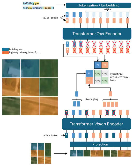
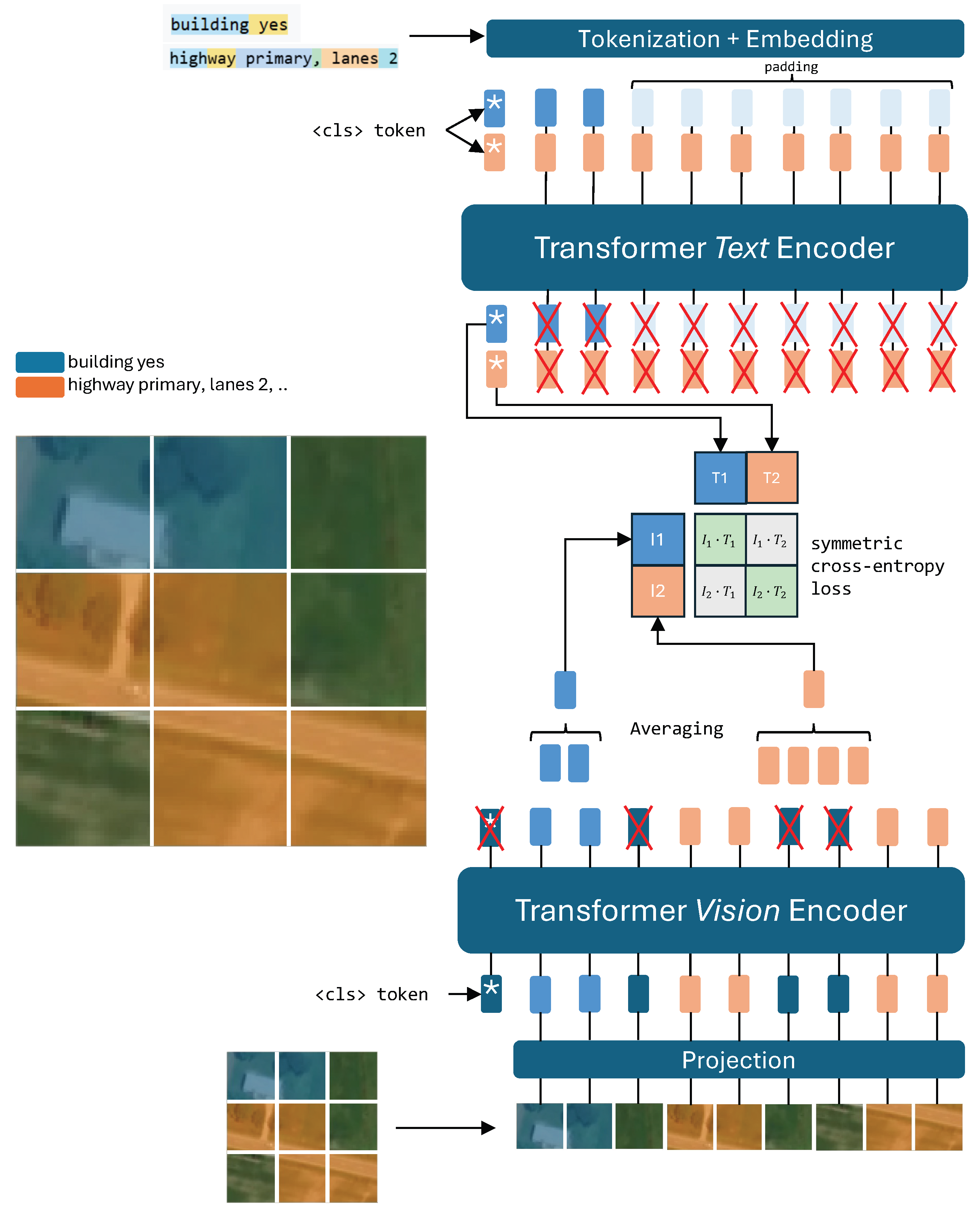
Figure 1 provides a schematic overview of this process.

Figure 1. Our proposed patch-level training method. Visual patches corresponding to OSM annotations are extracted from the vision encoder and their features are aggregated per tag type. These aggregated features are then contrasted with text embeddings from the text encoder.

3.2. Modified Vision Transformer Architecture

The CLIP model employs a Vision Transformer (ViT) that processes images through patch embedding and transformer encoding, ultimately producing a global vector representation for image understanding. We modify its inner mechanism to preserve and leverage spatial information:

1.

Patch Embedding: The input image I is divided into a set of non-overlapping square patches. Each patch is linearly projected to obtain patch embeddings $\mathbf{E}\in {\mathbb{R}}^{M\times D}$, where M is the number of patches and D is the embedding dimension.

2.

Transformer Encoding: A special [CLS] token embedding is prepended to the set of patch embeddings, and the whole list is processed through L transformer layers with self-attention.

3.

Patch Feature Extraction: At the final transformer layer, we deviate from the standard CLIP architecture by discarding the [CLS] token embedding and retaining all patch embeddings. This yields a final embedding matrix ${\mathbf{F}}_v\in {\mathbb{R}}^{M\times D}$, where each row ${\mathbf{f}}_v^j$ represents the D-dimensional feature vector for patch j. By doing so, we retain spatial information at the patch level without collapsing into a single global representation.

3.3. Patch-Based Contrastive Learning with Feature Aggregation

During training, we operate on batches of B images, where each image is associated with multiple OSM annotations. Among all images in a batch, we identify the set of unique descriptions (e.g., “building residential”, “highway primary”). For each unique description $t_k$, we collect all patches from all images that are associated with that description, forming a set ${\mathcal{P}}_k=\{p_{i,j}\mid \mathrm{patch}j\mathrm{in}\mathrm{image}i\mathrm{contains}\mathrm{tag}{t}_k\}$. To smooth training and reduce noise, at the last transformer layer, we aggregate the embeddings of all patches sharing the same description across the entire batch. Specifically, we aggregate patches by averaging their embeddings:

$${\mathbf{v}}_k={\displaystyle \frac{1}{|{\mathcal{P}}_k|}}\sum _{p\in {\mathcal{P}}_k}{\mathbf{f}}_v^p$$

(2)

where ${\mathbf{f}}_v^p$ is the feature vector for patch p and $|{\mathcal{P}}_k|$ is the number of patches associated with description $t_k$ in the batch.

Note that during training, to avoid ambiguity, each patch is assigned to at most one tag per batch. When a patch falls within the footprint of multiple geographic features, we resolve the conflict by prioritizing tags with fewer associated patches in the batch, thereby favoring rarer geographic concepts. Formally, tags are sorted in ascending order of $\left|\varphi \right(t_k\left)\right|$, and each patch index is assigned to the first tag that claims it. This design is motivated by the information content of OSM tags: frequent, ubiquitous tags (e.g., building, highway) are spatially pervasive but weakly discriminative, whereas rarer tags (e.g., barrier=gate, leisure=golf_course) denote specific, localized concepts that carry higher semantic information. Prioritizing the rarer tag when a patch is contested prevents common categories from dominating the supervision signal and encourages the model to learn the more informative, fine-grained concepts that would otherwise be masked. This rationale is analogous to inverse-frequency weighting schemes such as TF–IDF, which are widely used to emphasize informative terms over common ones. A systematic ablation of alternative conflict-resolution policies is left to future work.

Both the aggregated visual features and the text features are ${\ell }_2$-normalized before computing the contrastive loss:

$${\widehat{\mathbf{v}}}_k={\displaystyle \frac{{\mathbf{v}}_k}{\parallel {\mathbf{v}}_k{\parallel }_2}},{\widehat{\mathbf{t}}}_k={\displaystyle \frac{{\mathbf{t}}_k}{\parallel {\mathbf{t}}_k{\parallel }_2}}$$

(3)

The similarity matrix is then computed as $\mathbf{S}=\widehat{\mathbf{V}}{\widehat{\mathbf{T}}}^{\top }\in {\mathbb{R}}^{N\times N}$, scaled by a learnable temperature parameter $\tau$.

Each description $d_k$ is processed within the text encoder $f_{\mathrm{text}}(·)$ to obtain its textual embedding:

$${\mathbf{t}}_k=f_{\mathrm{text}}\left(d_k\right),$$

(4)

where $d_k$ denotes the textual description (e.g., “building residential”) and ${\mathbf{t}}_k\in {\mathbb{R}}^D$ is the corresponding text feature vector.

Let N denote the number of unique descriptions in a batch. After processing, we are left with two matrices: a visual feature matrix $\mathbf{V}\in {\mathbb{R}}^{N\times D}$ containing the aggregated patch features and a text feature matrix $\mathbf{T}\in {\mathbb{R}}^{N\times D}$ containing the corresponding text embeddings. We then apply the standard CLIP contrastive loss between these aligned visual and textual representations:

$${\mathcal{L}}_{OSM}={\displaystyle \frac{1}{2}}\left({\mathcal{L}}_{v2t}+{\mathcal{L}}_{t2v}\right)$$

(5)

where

$${\mathcal{L}}_{v2t}=-{\displaystyle \frac{1}{N}}{\displaystyle \sum _{k=1}^N}log{\displaystyle \frac{exp({\widehat{\mathbf{v}}}_k·{\widehat{\mathbf{t}}}_k/\tau )}{{\sum }_{j=1}^{N}exp({\widehat{\mathbf{v}}}_k·{\widehat{\mathbf{t}}}_j/\tau )}}$$

(6)

$${\mathcal{L}}_{t2v}=-{\displaystyle \frac{1}{N}}{\displaystyle \sum _{k=1}^N}log{\displaystyle \frac{exp({\widehat{\mathbf{t}}}_k·{\widehat{\mathbf{v}}}_k/\tau )}{{\sum }_{j=1}^{N}exp({\widehat{\mathbf{t}}}_k·{\widehat{\mathbf{v}}}_j/\tau )}}$$

(7)

and $\tau$ is the temperature parameter controlling the sharpness of the distribution. This formulation encourages the model to learn visual representations where patches depicting similar geographic features (as indicated by OSM tags) are embedded close to their corresponding textual descriptions while being separated from unrelated concepts.

3.4. Training Objective

Our training procedure consists of two stages: OSM-supervised pre-training and caption-based fine-tuning. In the pre-training stage, we optimize an OSM patch-level contrastive loss ${\mathcal{L}}_{\mathrm{OSM}}$ between aggregated patch features and OSM text embeddings. In the fine-tuning stage, we adapt the model to downstream tasks using the standard CLIP loss ${\mathcal{L}}_{\mathrm{CLIP}}$ on remote sensing captioning datasets.

Overall, the training objective can be expressed as

$$\mathcal{L}={\lambda }_{\mathrm{OSM}}{\mathcal{L}}_{\mathrm{OSM}}+{\lambda }_{\mathrm{CLIP}}{\mathcal{L}}_{\mathrm{CLIP}},$$

(8)

where ${\lambda }_{\mathrm{OSM}}$ and ${\lambda }_{\mathrm{CLIP}}$ control the relative contribution of OSM patch-level supervision and caption-level CLIP supervision. In practice, we optimize ${\mathcal{L}}_{\mathrm{OSM}}$ during the pre-training stage and ${\mathcal{L}}_{\mathrm{CLIP}}$ during the fine-tuning stage.

3.5. Training Strategy

We divide training into two phases: pre-training and fine-tuning. Pre-training represents our spatially aware training with OSM descriptions. Fine-tuning adapts the model to the downstream task and can differ depending on which downstream task is chosen.

1.

OSM pre-training: this represents our spatially aware training with OSM descriptions, which uses our patch-based contrastive loss with feature aggregation. The goal of pre-training is only to inject spatial awareness into visual and textual embeddings; therefore, the model must be adapted to downstream tasks through fine-tuning. Different fine-tuning schemes serve different downstream tasks.

2.

Fine-tuning: In this work, we fine-tune to adapt the model for zero-shot classification and image-text retrieval. We thus use the standard CLIP contrastive loss (that uses the [CLS] token embeddings) on a combination of existing remote sensing image captioning datasets (NWPU-RESISC45, RSICD, UCM, and SYDNEY). We demonstrate through our results that the knowledge absorbed in the pre-training stage allows the model to achieve higher scores, effectively demonstrating that it learns better representations.

4. Dataset Creation

Constructing geographically grounded supervision at scale requires aligning satellite imagery with structured spatial annotations. To achieve this, we build a large-scale dataset by combining satellite image tiles with OpenStreetMap vector features automatically projected onto ViT image patches. Every image is automatically associated with structured OSM annotations that describe the geographic features present within its bounds and mapped to specific image regions through a fully automated scraping and processing pipeline.

The dataset construction pipeline consists of five automated stages: geographic sampling and image acquisition, OSM querying and tag filtering, geometric processing, patch-mask generation, and text processing. The overall goal is to retain visually meaningful geographic annotations while reducing noise from incomplete, non-visual, or semantically irrelevant OSM metadata, ensuring that the resulting image–text pairs are both spatially accurate and suitable for contrastive representation learning.

Geographic sampling and image acquisition. Locations are uniformly sampled within the contiguous United States (latitude $\in [{25}^{°},{49}^{°}]$, longitude $\in [-{125}^{°},-{66}^{°}]$), chosen for its dense and consistent OSM coverage. For each sampled location, a square satellite image is downloaded from the Mapbox Satellite v9 API, covering a $250\times 250$ m area centered on the sampled point, providing a fixed spatial context for associating image content with OSM annotations.

OSM querying and tag filtering. For each satellite tile, the Overpass API is queried to retrieve all OSM nodes and ways located within the image bounding box, returning full geometry information including point, linear, and polygonal features. To reduce noise during scraping, untagged elements are discarded, and tag keys are validated against the OSM taginfo wiki database. Metadata categories unlikely to correspond to visible image content are removed, including references, imports, annotations, addresses, boundaries, underground or underwater features, and name-related attributes such as proper nouns or operator names. Open ways sharing endpoints and identical tags are merged to improve geometric consistency. A second post-processing stage further removes non-visual or weakly informative tags by applying an explicit blocklist of metadata keys (e.g., opening_hours, brand, population, voltage, maxspeed, start_date) and discarding malformed values. We deliberately do not impose a minimum-occurrence threshold: rather than discarding infrequent tags, we retain rare but visually informative concepts (e.g., barrier=gate, highway=turning_circle) and instead resolve tag overlaps at training time by prioritizing rarer tags (Section 3). This ensures that the final textual descriptions correspond to visual geographic concepts that can plausibly be learned from satellite imagery.

Geometric processing. The retained OSM features are projected from geographic coordinates into image pixel coordinates and processed according to their geometry type using the Shapely library. Closed ways are treated as polygons and intersected with the image bounding box, while open ways are clipped as line geometries. Point features are projected directly to their corresponding image locations. To reduce boundary artifacts, elements whose centers fall outside 97% of the image bounding box are discarded, and images without valid geographic elements after filtering are removed from the dataset.

Patch mask generation. The image is divided into a grid of ${(224/32)}^2=49$ cells matching the ViT-B/32 patch grid. For each geographic feature, the associated patch indices are determined according to geometry type: for nodes, the containing grid cell is identified via coordinate projection; for polygons, all grid cells intersecting the polygon footprint are identified; for lines, all grid cells intersecting any line segment are identified. The output is a JSON file mapping each tag string to its list of patch indices.

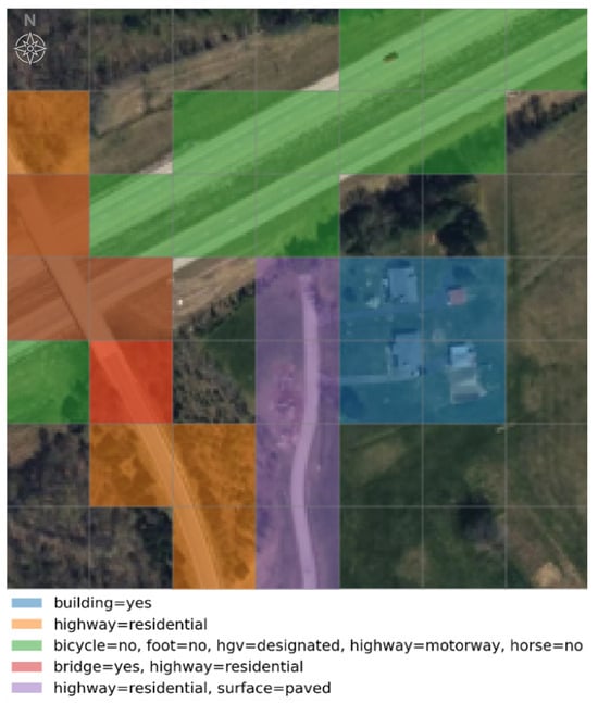
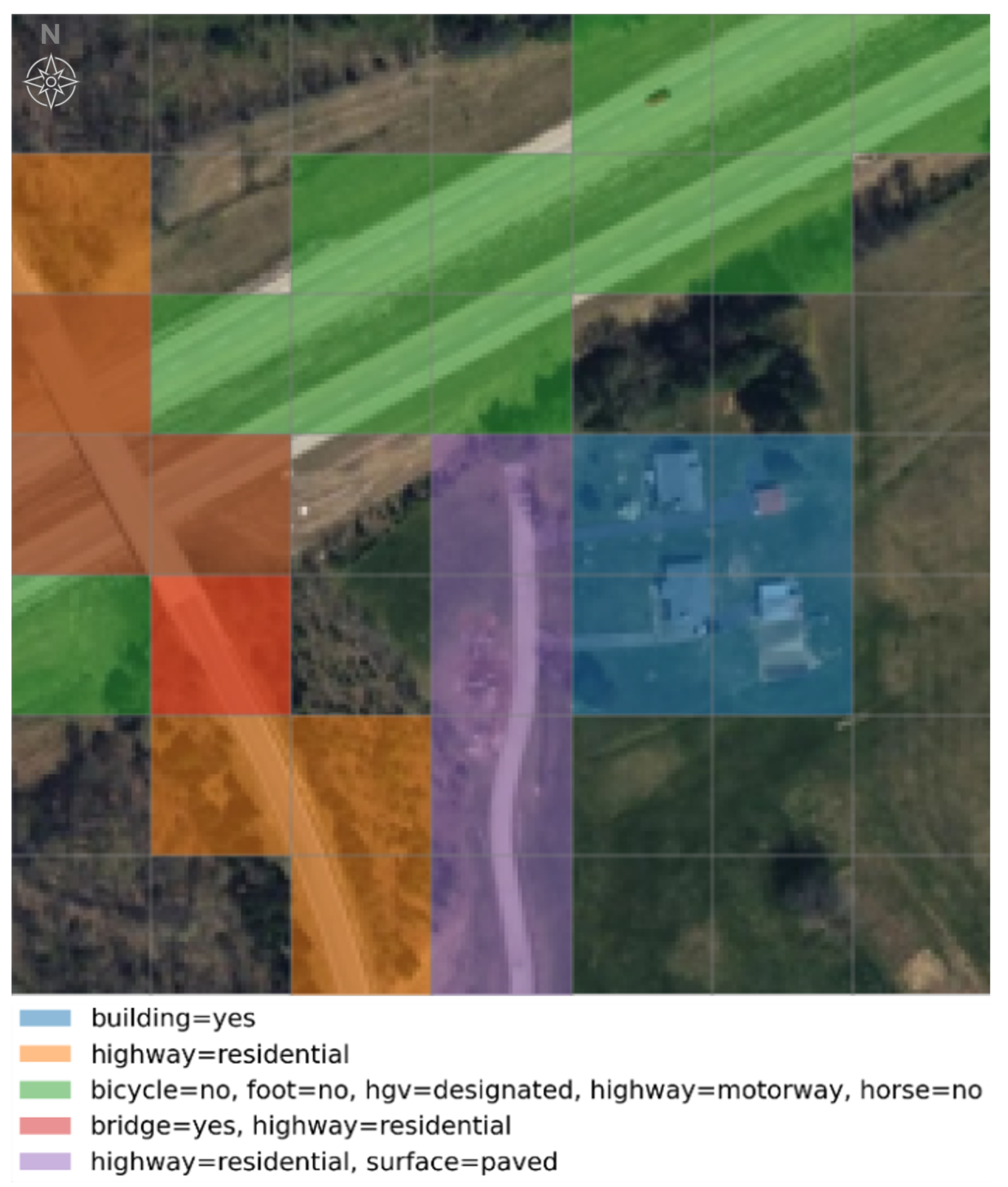
Text processing. Raw OSM tag syntax (key=value pairs within curly braces) is converted to plain text by removing special characters ({, }, ’, =, :, ,), producing human-readable descriptions such as “building residential” or “highway primary surface asphalt”. Figure 2 illustrates a representative sample with OSM features overlaid on the patch grid.

Figure 2. Visualization of a sample in our dataset. The satellite image ($224\times 224$ px) is overlaid with a $7\times 7$ grid of $32\times 32$ px patches (matching the ViT-B/32 patch grid, i.e., 49 patches per image); each colored grid patch represents an OSM feature, labeled with its corresponding textual annotation.

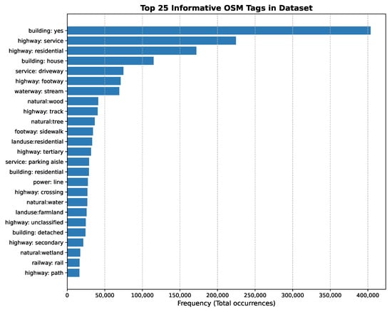
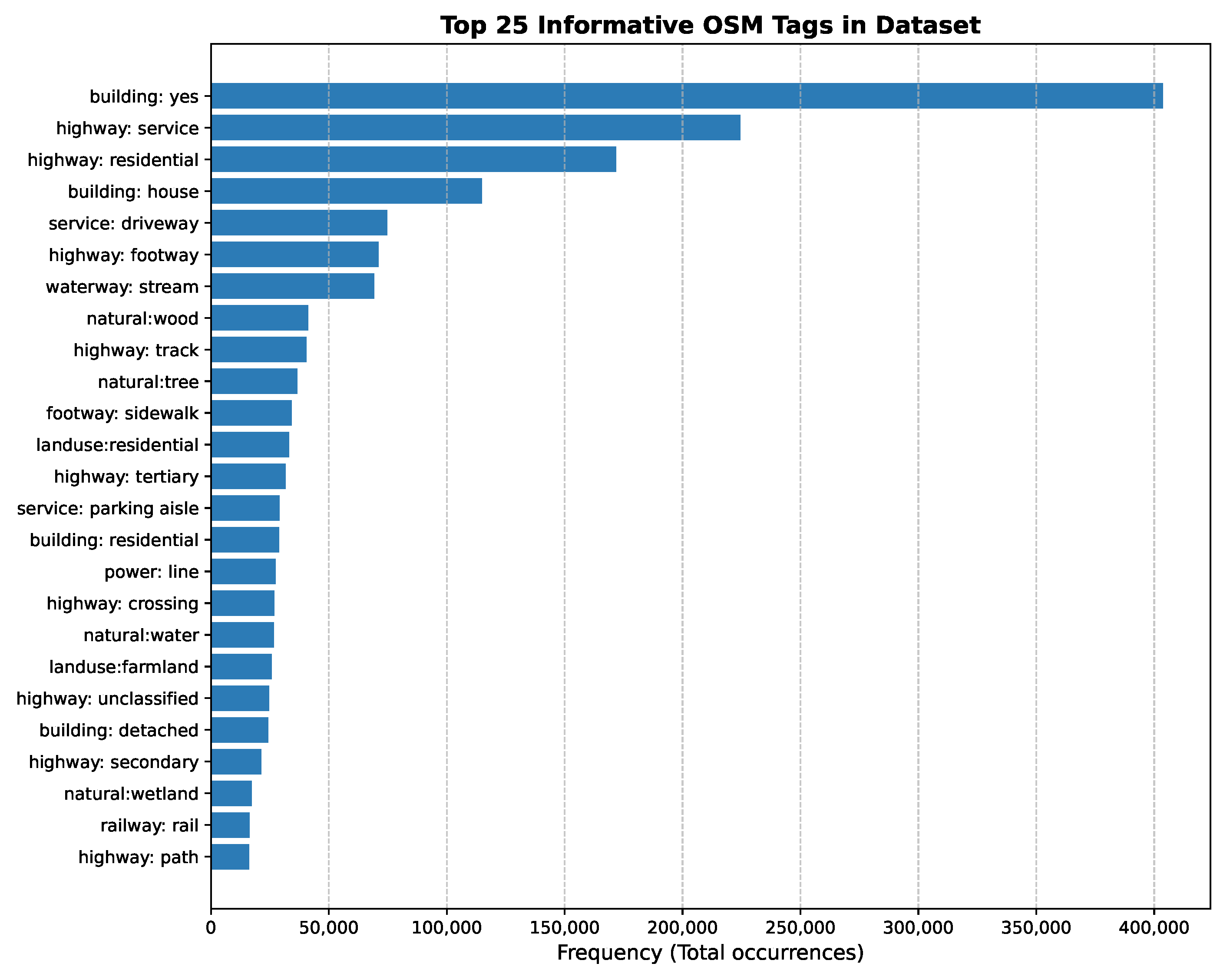
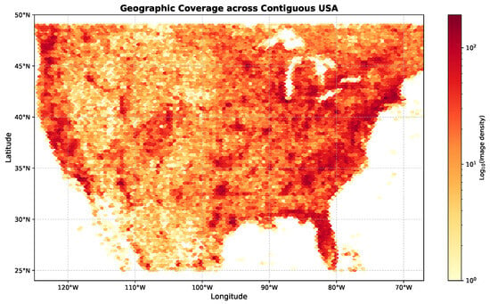
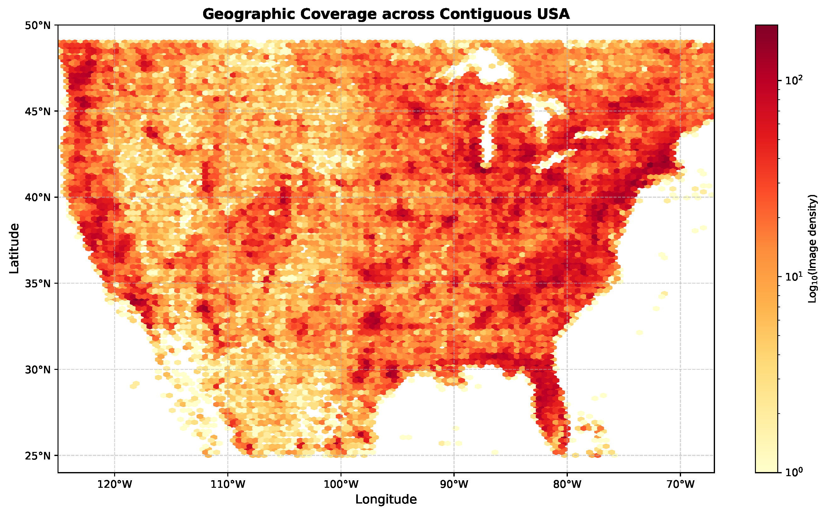
The resulting dataset contains 265,135 samples. Each sample consists of a satellite image and a structured JSON annotation file produced by the pipeline above, requiring no human labeling at any stage. The dataset is split using a 70/20/10 train/validation/test ratio. The effect of the filtering pipeline is substantial: starting from 16,118 unique tags (536 keys, ≈5.28 M tag instances) in the per-image metadata, the key-based filtering stage reduces the vocabulary to 4282 unique tags across 424 keys, of which 423 are semantic OSM categories (the remaining one being a synthetic spatial-position descriptor). The retained tag frequencies are strongly long-tailed (median of 5 occurrences per tag, with 27% of tags occurring only once), which is precisely why we retain rare tags rather than applying a frequency threshold. Figure 3 shows the distribution of the 25 most frequent OSM tags in the dataset, while Figure 4 illustrates the geographic coverage across the contiguous United States.

Figure 3. Distribution of the top 25 OpenStreetMap tags in our dataset, showing a diverse range of geographic features from road networks (highway) to land use types and building categories.

Figure 4. Geographic distribution of the dataset samples across the contiguous United States. The density map shows broad coverage with higher concentration in densely annotated urban and suburban regions.

5. Experimental Setup

Experiments in this paper consider the ViT-B/32 variant of the CLIP model.

5.1. Implementation Details

We trained our model on a single NVIDIA RTX 3090 GPU. We use the Adafactor optimizer [24] with a learning rate of $5\times {10}^{-5}$, weight decay of $0.05$, and batch size of 128 (with gradient accumulation over 2 steps for an effective batch size of 256). The model is trained for approximately 48 h during the pretraining stage. No data augmentation is applied during pretraining. All reported metrics are obtained from a single training run per configuration due to computational constraints on shared GPU resources. Investigating variance across multiple runs is left to future work.

5.2. Baseline Datasets

For evaluation, we perform fine-tuning using four well-established remote sensing image captioning datasets:

• NWPU-RESISC45 [25]: 31,500 images across 45 scene categories
• RSICD [26]: 10,921 images with 5 captions each
• UCM [27]: 2100 images across 21 land use categories
• SYDNEY [28]: 613 images across 7 categories

5.3. Evaluation and Compared Methods

We evaluate all models using the VT-RSBS benchmark (https://github.com/albertofrizzera/VT-RSBS (accessed on 2 June 2026)): 

1.

Classification: Zero-shot and linear probe classification accuracy on 13 remote sensing scene classification datasets. For zero-shot classification, all models are evaluated using the prompt template "a remote sensing image of a {class}", following the default configuration of the benchmark.

2.

Retrieval: Recall@K (K = 1, 5, 10, 50) for both image-to-text and text-to-image retrieval on 4 datasets.

All models, including the publicly released GeoRSCLIP ViT-B/32 checkpoint, are evaluated under this unified protocol to ensure a fair and consistent comparison. Specifically, all models share the exact same evaluation codebase, prompt template, and input image resolution ($224\times 224$ pixels) across all classification and retrieval benchmarks.

We compare six approaches:

• CLIP [1]: Original CLIP model released by OpenAI.
• RemoteCLIP [2]: CLIP model fine-tuned on remote sensing data, widely adopted as a strong remote sensing vision–language baseline.
• GeoRSCLIP [3]: A domain pre-trained vision–language model trained on the RS5M dataset, focused on global image–text alignment. Results are reported from the publicly released ViT-B/32 checkpoint evaluated under the same benchmark and prompt template used in this work.
• FT: CLIP model undergoing only the fine-tuning stage on the four captioning datasets. Establishes the benefit of domain fine-tuning alone.
• RS-PT+FT: CLIP pre-trained on our 265,135 satellite images using a generic caption (“a satellite image”) and the standard CLIP loss, then fine-tuned. This baseline isolates the effect of additional domain-specific images from the effect of OSM geographic supervision.
• OSM-PT+FT (Ours): Our complete approach. CLIP is first pre-trained with the patch-level OSM loss, then fine-tuned with the standard CLIP loss.

Comparing FT, RS-PT+FT, and OSM-PT+FT allows us to isolate the contribution of OSM geographic supervision from the mere effect of additional training data.

5.4. Relation to GeoRSCLIP and LRSCLIP

GeoRSCLIP [3] and LRSCLIP [4] build on large-scale captioning datasets (RS5M, LRS2M) and focus on global image–text alignment for retrieval and zero-shot classification, whereas our framework targets patch-level geospatial grounding through OSM supervision.

Due to differences in objectives (global retrieval versus spatial grounding), supervision signals (caption-level versus OSM patch-level tags), and evaluation protocols (pure zero-shot versus OSM-pretraining followed by task-specific fine-tuning), direct quantitative comparison is not always meaningful. Therefore, we include GeoRSCLIP and LRSCLIP results primarily as contextual references representing the state-of-the-art in remote sensing VLMs, rather than as direct competitors in a unified training pipeline. Instead, we position OSM-CLIP as complementary to GeoRSCLIP/LRSCLIP: it targets fine-grained geospatial grounding using structured geographic priors, rather than solely improving global alignment on captioning corpora. Table 1 summarizes the qualitative differences in capabilities across these models.

Table 1. Qualitative comparison of capabilities across remote sensing vision–language models.

Method	Retrieval	Classification	OSM-Aware	Spatial Grounding	Open-Vocabulary
RemoteCLIP	✓	✓	–	–	Partial
GeoRSCLIP	✓	✓	–	–	Partial
LRSCLIP	✓	✓	–	–	✓
OSM-CLIP (Ours)	Partial	Partial	✓	✓	✓

✓ = full support; Partial = limited support; – = not supported.

6. Results and Discussion

This section presents a comprehensive evaluation of OSM-CLIP across zero-shot classification, linear probe classification, and cross-modal retrieval benchmarks. We first report overall performance across all 13 classification and 4 retrieval datasets, then analyze the contribution of OSM supervision through a controlled ablation study, and finally provide qualitative evidence of the model’s spatial grounding capabilities.

Table 2 and Table 3 present zero-shot classification results across all 13 remote sensing datasets; Table 4 and Table 5 report the corresponding linear probe results. The performance delta between our OSM-PT+FT and RemoteCLIP is included in the second part of each pair.

Table 2. Zero-shot Classification Performance (%) on the first seven benchmark datasets (Part 1/2). Results continue in Table 3. All models are evaluated using the prompt template "a remote sensing image of a {class}"; GeoRSCLIP results use the publicly released ViT-B/32 checkpoint. Bold and underline denote first and second best among directly comparable methods (GeoRSCLIP is reported as a contextual reference; see Section 5).

Method	UCM	WHU_RS19	RSSCN7	SIRI_WHU	RESISC45	RSI_CB128	RSI_CB256
CLIP	64.76	80.60	65.00	51.67	74.38	24.45	34.08
RemoteCLIP	87.62	94.53	52.86	60.83	79.43	27.96	41.56
GeoRSCLIP	71.19	86.07	79.82	52.08	75.10	26.60	43.70
FT	95.00	96.52	73.57	66.46	87.14	33.97	50.83
RS-PT+FT	94.29	95.52	71.96	63.54	67.24	32.17	46.89
OSM-PT+FT (Ours)	96.90	96.02	76.43	72.29	92.62	34.09	46.32
Δ (Ours–RemoteCLIP)	+9.28	+1.49	+23.57	+11.46	+13.19	+6.13	+4.76

Table 3. Zero-shot Classification Performance (%) on the remaining six benchmark datasets and overall average (Part 2/2). Avg. is computed over all 13 datasets in Table 2 and Table 3. Notation as in Table 2.

Method	EuroSAT	PatternNet	OPTIMAL_31	MLRSNet	RSICD	RSITMD	Avg.
CLIP	40.37	58.88	76.08	51.23	59.74	53.54	56.52
RemoteCLIP	39.46	58.67	71.77	53.63	84.72	80.75	64.14
GeoRSCLIP	47.41	72.50	76.34	63.99	67.06	58.63	63.88
FT	52.43	72.22	98.39	71.98	84.63	81.64	74.21
RS-PT+FT	46.28	73.03	98.66	73.48	86.46	77.21	71.29
OSM-PT+FT (Ours)	51.87	69.34	98.92	71.65	86.09	81.86	74.95
Δ (Ours–RemoteCLIP)	+12.41	+10.67	+27.15	+18.02	+1.37	+1.11	+10.81

Table 4. Linear Probe Classification Performance (%) on the first seven benchmark datasets (Part 1/2). Results continue in Table 5. Notation as in Table 2.

Method	UCM	WHU_RS19	RSSCN7	SIRI_WHU	RESISC45	RSI_CB128	RSI_CB256
CLIP	95.00	99.00	94.29	94.17	98.10	98.19	98.95
RemoteCLIP	99.29	98.51	94.29	96.67	98.76	98.72	99.37
GeoRSCLIP	99.29	100.00	96.07	96.67	98.76	99.09	99.23
FT	99.29	100.00	94.29	95.42	99.81	98.56	99.25
RS-PT+FT	99.29	99.50	94.11	97.08	99.86	98.15	99.21
OSM-PT+FT (Ours)	99.76	100.00	95.36	96.67	99.90	98.84	99.47
Δ (Ours–RemoteCLIP)	+0.47	+1.49	+1.07	0.00	+1.14	+0.12	+0.10

Table 5. Linear Probe Classification Performance (%) on the remaining six benchmark datasets and overall average (Part 2/2). Avg. is computed over all 13 datasets in Table 4 and Table 5. Notation as in Table 2.

Method	EuroSAT	PatternNet	OPTIMAL_31	MLRSNet	RSICD	RSITMD	Avg.
CLIP	95.74	98.83	94.89	93.75	95.33	93.14	96.11
RemoteCLIP	96.39	99.39	94.09	94.64	96.07	95.35	97.04
GeoRSCLIP	97.43	99.34	97.04	95.87	96.61	95.35	97.75
FT	96.63	99.06	98.92	94.93	95.88	95.35	97.49
RS-PT+FT	96.80	99.19	99.73	95.13	96.43	97.35	97.83
OSM-PT+FT (Ours)	97.06	99.18	100.00	95.43	95.52	97.35	97.96
Δ (Ours–RemoteCLIP)	+0.67	−0.21	+5.91	+0.79	−0.55	+2.00	+0.92

OSM-PT+FT achieves the best average zero-shot performance (74.95%, Table 3), with an improvement of +10.81% over RemoteCLIP. For reference, GeoRSCLIP ViT-B/32 evaluated under the same benchmark and prompt template achieves a zero-shot average of 63.88%. GeoRSCLIP focuses primarily on global image–text representation learning, whereas OSM-CLIP explicitly targets spatially grounded geographic supervision through patch-level OSM alignment.

In the linear-probe setting (Table 5), OSM-PT+FT also achieves the highest average performance at 97.96%, compared with 97.04% for RemoteCLIP and 97.75% for GeoRSCLIP, corresponding to a +0.92% improvement. The larger gain in zero-shot classification compared to linear probe is consistent with this design choice: OSM patch-level supervision primarily improves the quality of the pretrained image–text alignment, which is most directly tested under zero-shot conditions, while the linear probe setting allows a learned classifier to partially compensate for weaker representations.

The RS-PT+FT ablation also sheds light on why generic domain pre-training can hurt zero-shot performance. During RS-PT, each satellite image is paired with the same generic caption (“a satellite image”), forcing the model to align diverse visual content to an almost non-discriminative text representation. This encourages the image encoder to collapse semantically distinct scenes toward a shared textual prototype, weakening the global image–text structure that zero-shot classification relies on. Fine-tuning partially recovers discriminative power on the downstream datasets, but the damage to the global alignment learned during pre-training explains why RS-PT+FT underperforms the FT baseline in zero-shot accuracy despite having seen more satellite imagery. This behavior is consistent with the dataset-level gains: the largest zero-shot improvements over RemoteCLIP occur on OPTIMAL_31 (+27.15%), RSSCN7 (+23.57%), and MLRSNet (+18.02%), where many scene categories correspond directly to well-defined geographic structures explicitly represented in OSM (e.g., airports, industrial facilities, agricultural fields, major road networks). Because OSM-PT+FT pre-trains the model to recognize these structures at the patch level and to associate them with their textual tags, the learned representations transfer especially well to benchmarks whose label space overlaps with OSM semantics.

Importantly, the RS-PT+FT baseline serves as the direct and fair ablation to isolate the benefits of the proposed patch-level OSM supervision. Since RS-PT+FT and OSM-PT+FT share the exact same pre-training satellite images (265,135 samples), training epochs, and subsequent fine-tuning protocol, the performance gap between them is strictly attributable to the OSM-derived spatial semantic supervision rather than the pre-training data volume. Furthermore, we observe that OSM-PT+FT does not achieve the top score on all individual benchmarks. Specifically, on RSI_CB256, the baseline FT (50.83%) outperforms OSM-PT+FT (46.32%), and on PatternNet, RS-PT+FT (73.03%) slightly exceeds OSM-PT+FT (69.34%). This occurs because these datasets contain highly specialized visual classes (e.g., specific plane models or texture-driven land cover types) that do not correspond directly to standard OSM tags (like ‘highway’ or ‘building’). In these cases, forcing the model’s patches to align with mismatched OSM tags during pre-training introduces semantic noise, which slightly degrades zero-shot accuracy compared to generic or fine-tuning-only baselines. Conversely, OSM supervision is highly effective when downstream classes have clear geographic counterparts represented in OSM.

Table 6 and Table 7 show the detailed retrieval results on four benchmark datasets for text-to-image and image-to-text tasks, respectively, with performance deltas compared to RemoteCLIP.

Table 6. Text-to-Image Retrieval Performance (%). Notation as in Table 2.

Method	UCM	RSICD	RSITMD	SYDNEY	Avg.
R@1
CLIP	8.57	5.75	8.76	12.07	8.79
RemoteCLIP	17.62	11.95	18.63	13.45	15.41
GeoRSCLIP	14.10	8.18	12.04	15.86	12.55
FT	15.62	11.56	19.96	19.31	16.61
RS-PT+FT	16.67	12.86	22.79	21.38	18.43
OSM-PT+FT (Ours)	17.52	14.22	30.84	19.31	20.47
Δ (Ours–RemoteCLIP)	−0.10	+2.27	+12.21	+5.86	+5.06
R@5
CLIP	36.67	17.22	27.70	41.03	30.66
RemoteCLIP	61.43	34.88	52.30	52.41	50.26
GeoRSCLIP	50.95	25.27	37.52	49.31	40.76
FT	58.76	34.62	53.36	55.86	50.65
RS-PT+FT	61.43	36.52	56.50	58.97	53.35
OSM-PT+FT (Ours)	62.10	38.19	65.66	63.79	57.44
Δ (Ours–RemoteCLIP)	+0.67	+3.31	+13.36	+11.38	+7.18
R@10
CLIP	60.57	28.64	42.43	69.31	50.24
RemoteCLIP	93.81	50.91	71.11	74.48	72.58
GeoRSCLIP	80.76	37.64	54.29	72.41	61.28
FT	93.71	51.60	74.07	75.86	73.81
RS-PT+FT	93.43	53.65	74.60	81.03	75.68
OSM-PT+FT (Ours)	94.76	54.93	79.38	80.69	77.44
Δ (Ours–RemoteCLIP)	+0.95	+4.02	+8.27	+6.21	+4.86

Table 7. Image-to-Text Retrieval Performance (%). Notation as in Table 2.

Method	UCM	RSICD	RSITMD	SYDNEY	Avg.
R@1
CLIP	10.00	4.85	9.51	13.79	9.54
RemoteCLIP	20.48	17.11	25.44	22.41	21.36
GeoRSCLIP	16.67	11.07	16.37	17.24	15.34
FT	17.62	15.28	21.90	18.97	18.44
RS-PT+FT	21.90	15.46	26.77	22.41	21.63
OSM-PT+FT (Ours)	24.76	16.74	38.72	20.69	25.23
Δ (Ours–RemoteCLIP)	+4.28	−0.37	+13.28	−1.72	+3.87
R@5
CLIP	28.57	14.18	22.79	41.38	26.73
RemoteCLIP	53.81	37.15	49.78	48.28	47.26
GeoRSCLIP	46.67	26.08	31.19	43.10	36.76
FT	53.81	32.48	45.58	56.90	47.19
RS-PT+FT	59.05	36.51	51.77	55.17	50.62
OSM-PT+FT (Ours)	60.00	35.86	63.50	55.17	53.63
Δ (Ours–RemoteCLIP)	+6.19	−1.29	+13.72	+6.89	+6.37
R@10
CLIP	52.38	24.06	33.85	55.17	41.37
RemoteCLIP	80.00	50.87	63.94	58.62	63.36
GeoRSCLIP	70.95	37.42	44.69	62.07	53.78
FT	80.48	44.28	61.50	74.14	65.10
RS-PT+FT	87.14	48.03	67.26	72.41	68.71
OSM-PT+FT (Ours)	86.19	50.41	76.11	75.86	72.14
Δ (Ours–RemoteCLIP)	+6.19	−0.46	+12.17	+17.24	+8.78

OSM-PT+FT achieves the strongest average retrieval performance across all metrics, with T2I R@1 of 20.47 and I2T R@1 of 25.23, while OSM-PT+FT does not consistently outperform RemoteCLIP on every individual retrieval configuration, the average gains confirm the benefit of OSM geographic supervision.

The largest retrieval gains are observed on RSITMD, with improvements of +12.21 percentage points in text-to-image R@1 and +13.28 in image-to-text R@1 over RemoteCLIP (Table 6 and Table 7). RSITMD includes relatively long and compositional scene descriptions that refer to multiple co-occurring geographic elements within the same image. In this setting, a purely global image–text representation is often insufficient to resolve which part of the image corresponds to which phrase, leading to ambiguous alignments. By contrast, OSM-PT+FT explicitly learns to associate textual concepts with localized regions through patch-level supervision, which better matches the fine-grained, multi-object nature of RSITMD captions and explains the particularly strong gains on this dataset.

The RS-PT+FT ablation reveals an important nuance: unlike zero-shot classification, retrieval metrics for RS-PT+FT (T2I R@1: 18.43; I2T R@1: 21.63) do exceed the FT baseline (16.61; 18.44), suggesting that domain-specific pre-training images provide some benefit for retrieval tasks. However, OSM-PT+FT consistently and substantially outperforms RS-PT+FT across all retrieval metrics, demonstrating that OSM geographic supervision provides gains well beyond those achievable with generic pre-training data alone.

Taken together with the zero-shot results, the RS-PT+FT ablation confirms a clear pattern: generic domain pre-training introduces a trade-off—it helps retrieval but hurts zero-shot classification—while OSM-supervised pre-training improves both task types consistently. This validates that the performance gains of OSM-PT+FT stem from the quality and geographic specificity of the supervision signal, not merely from additional training data.

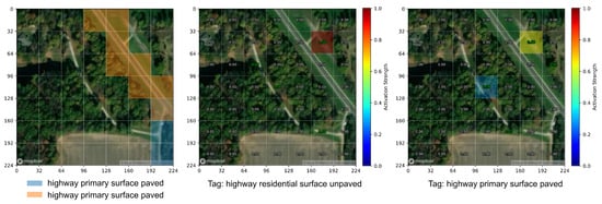
Figure 5 provides a qualitative evaluation of the model’s spatial grounding capabilities on unseen test data. The left panel visualizes the OSM ground truth where a primary paved road and an unpaved residential branch are present. The center and right panels show the model’s patch activations when queried with the respective tags. The model successfully isolates the specific image regions corresponding to each geographic class, even when multiple classes coexist within the same scene. This confirms that the patch-level contrastive loss effectively teaches the model to associate textual descriptions with their precise spatial locations, rather than merely learning global image-level associations.

Figure 5. Qualitative results on unseen test data. The left panel shows the Ground Truth visualization of OSM elements. The center and right panels show model activation maps for two different tag combinations on the same image. The model correctly distinguishes the primary paved road from the unpaved residential branch, demonstrating precise spatial grounding of co-occurring multi-attribute geographic features.

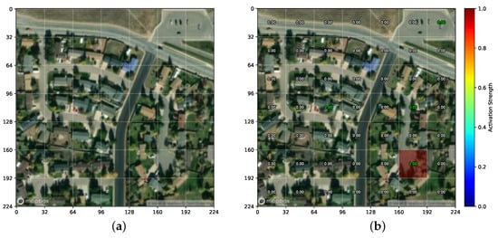
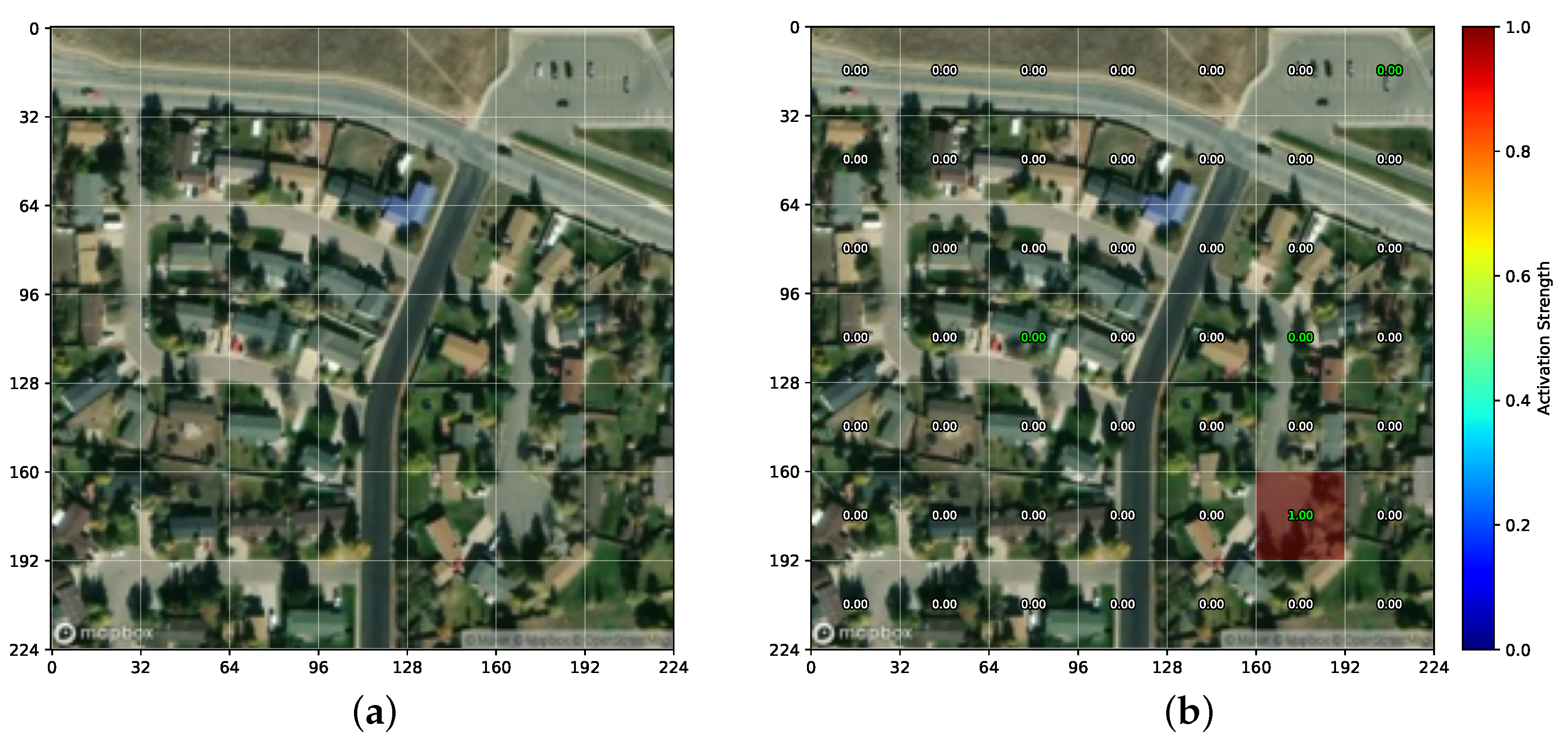
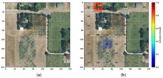
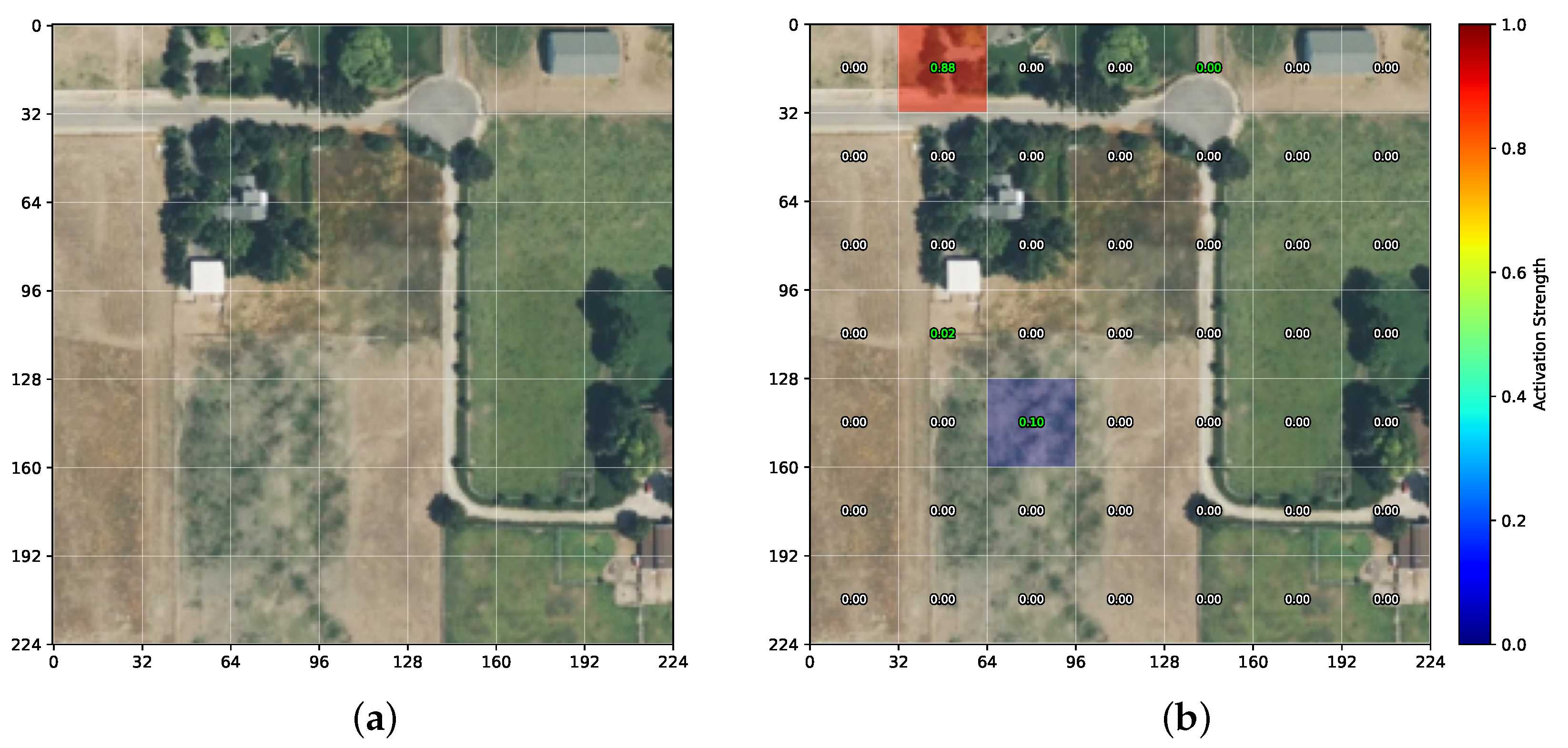
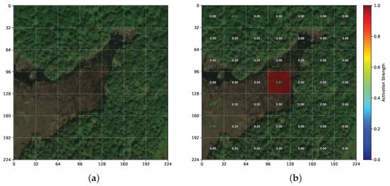
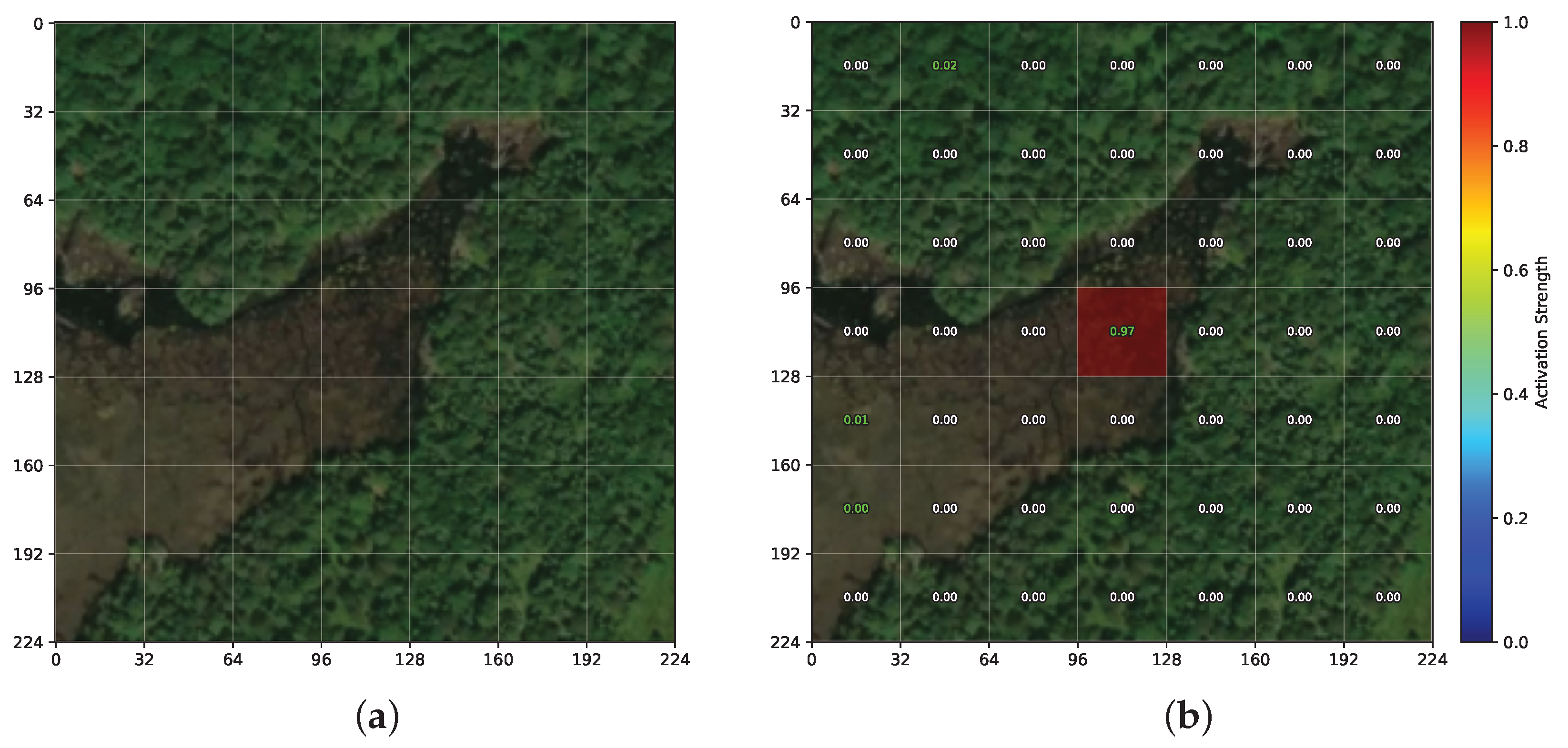
Figure 6, Figure 7 and Figure 8 present additional qualitative examples on unseen test data, including both successful localizations and a failure case.

Figure 6. Successful localization of a rare, small-scale road feature on a suburban scene (unseen test data). (a) Satellite image; (b) activation map for highway=turning_circle. The model precisely localizes this cul-de-sac with activation 1.00 on the correct patch (bottom-right), where a residential street ending in a turning circle is visible. This demonstrates fine-grained spatial grounding of uncommon geographic concepts.

Figure 7. Successful localization of a rare tag. (a) Satellite image; (b) activation map for barrier=gate (activation 0.89). The model correctly identifies the barrier gate (a low-frequency category) in the top-left patch where a driveway entrance is visible, demonstrating that the patch-level loss enables learning of uncommon geographic concepts.

Figure 8. Failure case: semantic confusion between similar categories. (a) Satellite image; (b) activation map for natural=water (activation 0.97). The image contains both natural=wetland and natural=water annotations. The model activates “natural water” on a central patch that corresponds to the wetland area rather than the water body (located in the upper-right region). This illustrates the difficulty of distinguishing visually similar geographic categories from satellite imagery alone.

Ablation Study: Isolating the Contribution of OSM Supervision

To assess statistical robustness despite a single training run, we computed 95% bootstrap confidence intervals (N = 1000 resamples with replacement) on all evaluation metrics for both OSM-PT+FT and RemoteCLIP under the same protocol. The macro-average zero-shot accuracy of OSM-PT+FT is 74.96% [74.34, 75.56] compared to 64.14% [63.33, 64.92] for RemoteCLIP; on RSITMD retrieval, T2I R@1 is 30.80% [28.85, 32.83] vs. 18.63% [17.12, 20.22], and I2T R@1 is 38.50% [34.29, 43.14] vs. 25.44% [21.46, 29.21]. All confidence intervals are non-overlapping, confirming that the reported gains are statistically significant and not attributable to random fluctuations. We note that bootstrapped test-set confidence intervals assess the stability of evaluation metrics but do not capture training variance arising from different random initializations; repeated training runs with different seeds remain a valuable direction for future work.

To disentangle the effect of OSM geographic supervision from the effect of additional training data, we compare three pre-training strategies sharing the same fine-tuning stage: (i) FT, which applies no pre-training; (ii) RS-PT+FT, which pre-trains on the same 265,135 satellite images using a generic caption (“a satellite image”); and (iii) OSM-PT+FT (ours), which pre-trains with the patch-level OSM contrastive loss. Table 8 summarizes the average performance across all benchmarks.

Table 8. Ablation study: average performance across all benchmarks for the three pre-training strategies. ZS = zero-shot classification; LP = linear probe classification; T2I and I2T = text-to-image and image-to-text retrieval R@1. All variants share the same fine-tuning stage; only the pre-training signal differs.

Method	ZS Avg. (%)	LP Avg. (%)	T2I R@1 (%)	I2T R@1 (%)
FT	74.21	97.49	16.61	18.44
RS-PT+FT	71.29	97.83	18.43	21.63
OSM-PT+FT (Ours)	74.95	97.96	20.47	25.23

Bold and underline denote first and second best, respectively.

RS-PT+FT degrades zero-shot classification relative to FT (71.29 vs. 74.21%) while slightly improving retrieval, confirming that exposure to additional satellite images without semantic supervision introduces a trade-off rather than a consistent benefit. As discussed above, the generic RS-PT caption ("a satellite image") weakens the global image–text structure that zero-shot classification relies on, explaining this trade-off. OSM-PT+FT is the only variant that improves over FT on all four metrics, confirming that OSM patch-level supervision, not pre-training data volume, drives the consistent gains.

7. Limitations

The current study has several limitations that should be acknowledged. First, our dataset is constructed exclusively from United States OSM data, which may introduce geographic bias due to differences in urban planning styles, vegetation types, and building materials across regions. The generalization to other parts of the world, particularly developing countries where both OSM coverage and visual landscapes differ significantly, remains to be validated. Second, the fixed patch size of $32\times 32$ pixels may not optimally capture geographic features of varying spatial extents. Third, OSM data quality varies by region, and our current pipeline does not explicitly account for incomplete or unverified annotations. Specifically, community-driven annotations are subject to uneven coverage (with dense annotations in urban areas and sparse metadata in rural regions), potentially introducing geographic sampling bias during pre-training. Furthermore, there is a risk of spatial misalignment between OSM vector geometries and high-resolution satellite imagery due to projection errors, as well as a potential temporal mismatch between satellite imagery acquisition dates and OSM annotation timestamps, which could lead to inconsistent image-text pairs in areas undergoing rapid change. Finally, the patch aggregation strategy based on simple averaging may be suboptimal, as patches labeled with a given tag (e.g., “highway”) may contain significant background content.

8. Conclusions

This paper presents OSM-CLIP, a framework that explores the potential of OpenStreetMap (OSM) as a regionally scalable source of patch-level geographic supervision for remote sensing vision–language models. By automatically mapping OSM vector features onto ViT image patches and training with a patch-level contrastive loss, OSM-CLIP learns spatially grounded representations without any manual annotation effort. A controlled ablation confirms these gains stem from the OSM supervision signal rather than added training data.

Key findings and contributions include:

• A scalable, annotation-free pipeline that automatically constructs over 265,000 satellite image–OSM patch-level pairs in the United States.
• A patch-level geographic supervision framework achieving an average improvement of +10.81% in zero-shot classification and +5.06%/+3.87% in text-to-image/image-to-text retrieval (R@1) over RemoteCLIP across 13 classification and 4 retrieval benchmarks.
• A controlled ablation study isolating the contribution of OSM supervision: pre-training with generic captions on the same satellite images degrades zero-shot performance (71.29% vs. 74.21% for FT-only), confirming that geographic specificity—not data volume—is the key factor.
• Public release of the dataset, pre-trained model weights, and training pipeline to support reproducibility.

While the current work focuses on demonstrating the viability of OSM as a patch-level supervision source, it also opens several promising directions for future research. Future work will explore: (1) extending the dataset to global OSM coverage across geographically diverse regions with multilingual tag support, (2) scaling to larger architectures (ViT-B/16, ViT-L/14), (3) incorporating data augmentation while preserving geographic patch alignment, (4) adaptive multi-scale patch processing for geographic features of varying spatial extents, (5) applying the learned representations to dense prediction tasks such as semantic segmentation and change detection, (6) replacing simple patch-feature averaging with attention-based aggregation mechanisms to better isolate geographic features from background content, (7) exploring soft multi-label patch assignment weighted by spatial coverage as an alternative to the current single-tag constraint, (8) leveraging large language models to expand concise OSM tags into richer natural language descriptions for pre-training, (9) introducing an explicit background class for unlabeled patches to improve discriminative power, and (10) integrating temporal reliability scores from OSM metadata to down-weight outdated or uncertain annotations during training.

References

- Radford, A.; Kim, J.W.; Hallacy, C.; Ramesh, A.; Goh, G.; Agarwal, S.; Sastry, G.; Askell, A.; Mishkin, P.; Clark, J.; et al. Learning Transferable Visual Models from Natural Language Supervision. In Proceedings of the 38th International Conference on Machine Learning, Virtual, 18–24 July 2021; pp. 8748–8763. [Google Scholar]
- Liu, F.; Chen, D.; Guan, Z.; Zhou, X.; Zhu, J.; Ye, Q.; Fu, L.; Zhou, J. RemoteCLIP: A Vision Language Foundation Model for Remote Sensing. IEEE Trans. Geosci. Remote Sens. 2024, 62, 5622216. [Google Scholar] [CrossRef] [Scilit]
- Zhang, Z.; Zhao, T.; Guo, Y.; Yin, J. RS5M and GeoRSCLIP: A Large-Scale Vision-Language Dataset and a Large Vision-Language Model for Remote Sensing. IEEE Trans. Geosci. Remote Sens. 2024, 62, 5642123. [Google Scholar] [CrossRef] [Scilit]
- Chen, W.; Chen, J.; Deng, Y.; Chen, J.; Feng, Y.; Xi, Z.; Liu, D.; Li, K.; Meng, Y. LRSCLIP: A Vision-Language Foundation Model for Aligning Remote Sensing Image with Longer Text. arXiv 2025, arXiv:2503.19311. [Google Scholar]
- Li, X.; Wen, C.; Hu, Y.; Zhou, N. RS-CLIP: Zero Shot Remote Sensing Scene Classification via Contrastive Vision-Language Supervision. Int. J. Appl. Earth Obs. Geoinf. 2023, 124, 103497. [Google Scholar] [CrossRef] [Scilit]
- Dong, S.; Wang, L.; Du, B.; Meng, X. ChangeCLIP: Remote Sensing Change Detection with Multimodal Vision-Language Representation Learning. ISPRS J. Photogramm. Remote Sens. 2024, 208, 53–69. [Google Scholar] [CrossRef] [Scilit]
- Marimo, C.T.; Blumenstiel, B.; Nitsche, M.; Jakubik, J.; Brunschwiler, T. Beyond the Visible: Multispectral Vision-Language Learning for Earth Observation. arXiv 2025, arXiv:2503.15969. [Google Scholar]
- Wang, Z.; Prabha, R.; Huang, T.; Wu, J.; Rajagopal, R. SkyScript: A Large and Semantically Diverse Vision-Language Dataset for Remote Sensing. In Proceedings of the 2024 AAAI Conference on Artificial Intelligence, Vancouver, BC, Canada, 20–27 February 2024; pp. 5765–5773. [Google Scholar]
- Mall, U.; Hariharan, B.; Bala, K. Remote Sensing Vision-Language Foundation Models without Annotations via Ground Remote Alignment. In Proceedings of the Twelfth International Conference on Learning Representations, Vienna, Austria, 7–11 May 2024. [Google Scholar]
- Audebert, N.; Le Saux, B.; Lefèvre, S. Joint Learning from Earth Observation and OpenStreetMap Data to Get Faster Better Semantic Maps. In Proceedings of the IEEE Conference on Computer Vision and Pattern Recognition (CVPR), Honolulu, HI, USA, 21–26 July 2017; pp. 67–75. [Google Scholar]
- Usmani, M.; Bovolo, F.; Napolitano, M. Remote Sensing and Deep Learning to Understand Noisy OpenStreetMap. Remote Sens. 2023, 15, 4639. [Google Scholar] [CrossRef] [Scilit]
- Bai, L.; Zhang, X.; Wang, H.; Du, S. Integrating Remote Sensing with OpenStreetMap Data for Comprehensive Scene Understanding through Multi-Modal Self-Supervised Learning. Remote Sens. Environ. 2025, 318, 114573. [Google Scholar] [CrossRef] [Scilit]
- Liu, C.; Albrecht, C.M.; Wang, Y.; Zhu, X.X. CromSS: Cross-Modal Pre-Training with Noisy Labels for Remote Sensing Image Segmentation. IEEE Trans. Geosci. Remote Sens. 2024, 62, 4406517. [Google Scholar] [CrossRef] [Scilit]
- Bazi, Y.; Bashmal, L.; Al Rahhal, M.M.; Al Dayil, R.; Al Ajlan, N. Vision Transformers for Remote Sensing Image Classification. Remote Sens. 2021, 13, 516. [Google Scholar] [CrossRef] [Scilit]
- Jiang, W.; Zhang, J.; Wang, D.; Zhang, Q.; Wang, Z.; Du, B. LeMeViT: Efficient Vision Transformer with Learnable Meta Tokens for Remote Sensing Image Interpretation. In Proceedings of the Thirty-Third International Joint Conference on Artificial Intelligence, Jeju, Republic of Korea, 3–9 August 2024; pp. 929–937. [Google Scholar]
- Wang, D.; Zhang, Q.; Xu, Y.; Zhang, J.; Du, B.; Tao, D.; Zhang, L. Advancing Plain Vision Transformer toward Remote Sensing Foundation Model. IEEE Trans. Geosci. Remote Sens. 2022, 61, 5607315. [Google Scholar] [CrossRef] [Scilit]
- Reed, C.J.; Gupta, R.; Li, S.; Brber, S.; Zhu, S.; Samber, N.; Ebrahimi, S.; Vishwanath, V.; Kornblith, S.; Darrell, T. Scale-MAE: A Scale-Aware Masked Autoencoder for Multiscale Geospatial Representation Learning. In Proceedings of the International Conference on Computer Vision, Paris, France, 2–6 October 2023; pp. 4088–4099. [Google Scholar]
- Cong, Y.; Khanna, S.; Meng, C.; Liu, P.; Rozi, E.; He, Y.; Burke, M.; Lobell, D.; Ermon, S. SatMAE: Pre-training Transformers for Temporal and Multi-Spectral Satellite Imagery. In Proceedings of the Advances in Neural Information Processing Systems 35 (NeurIPS), New Orleans, LA, USA, 28 November–9 December 2022; pp. 197–211. [Google Scholar]
- Yun, S.; Kim, S.; Han, D.; Song, H.; Song, J.; Hong, Y. Patch-Level Representation Learning for Self-Supervised Vision Transformers. In Proceedings of the 2022 IEEE/CVF Conference on Computer Vision and Pattern Recognition (CVPR), New Orleans, LA, USA, 18–24 June 2022; pp. 9534–9544. [Google Scholar]
- Jean, N.; Wang, S.; Samar, A.; Azzari, G.; Lobell, D.; Ermon, S. Tile2Vec: Unsupervised Representation Learning for Spatially Distributed Data. In Proceedings of the Thirty-Third AAAI Conference on Artificial Intelligence (AAAI-19), Honolulu, HI, USA, 27 January–1 February 2019; pp. 3967–3974. [Google Scholar]
- Li, W.; Chen, K.; Chen, H.; Shi, Z. GLCNet: Global-Local Contrastive Network for Self-Supervised Representation Learning in Remote Sensing. IEEE Trans. Geosci. Remote Sens. 2022, 60, 1–12. [Google Scholar] [CrossRef] [Scilit]
- Muhtar, D.; Zhang, X.; Xiao, P.; Li, Z.; Gu, F. CMID: A Unified Self-Supervised Learning Framework for Remote Sensing Image Understanding. IEEE Trans. Geosci. Remote Sens. 2023, 61, 5607817. [Google Scholar] [CrossRef] [Scilit]
- Zhang, J.; Wang, D.; Liu, Y.; Zhang, Q.; Du, B. Multimodal Contrastive Learning for Remote Sensing Image Feature Extraction Based on Relaxed Positive Samples. Sensors 2024, 24, 7719. [Google Scholar] [CrossRef] [Scilit] [PubMed]
- Shazeer, N.; Stern, M. Adafactor: Adaptive Learning Rates with Sublinear Memory Cost. In Proceedings of the 35th International Conference on Machine Learning, Stockholm, Sweden, 10–15 July 2018; pp. 4596–4604. [Google Scholar]
- Cheng, G.; Han, J.; Lu, X. Remote Sensing Image Scene Classification: Benchmark and State of the Art. Proc. IEEE 2017, 105, 1865–1883. [Google Scholar] [CrossRef] [Scilit]
- Lu, X.; Wang, B.; Zheng, X.; Li, X. Exploring Models and Data for Remote Sensing Image Caption Generation. IEEE Trans. Geosci. Remote Sens. 2018, 56, 2183–2195. [Google Scholar] [CrossRef] [Scilit]
- Yang, Y.; Newsam, S. Bag-of-Visual-Words and Spatial Extensions for Land-Use Classification. In Proceedings of the 18th SIGSPATIAL International Conference on Advances in Geographic Information Systems, San Jose, CA, USA, 2–5 November 2010; pp. 270–279. [Google Scholar]
- Zhang, X.; Wang, T.; Qi, J.; Lu, H.; Wang, G. Saliency Detection for Remote Sensing Images: A Survey. Remote Sens. 2021, 13, 5100. [Google Scholar] [CrossRef] [Scilit]
Disclaimer/Publisher’s Note: The statements, opinions and data contained in all publications are solely those of the individual author(s) and contributor(s) and not of MDPI and/or the editor(s). MDPI and/or the editor(s) disclaim responsibility for any injury to people or property resulting from any ideas, methods, instructions or products referred to in the content. |
© 2026 by the authors. Licensee MDPI, Basel, Switzerland. This article is an open access article distributed under the terms and conditions of the Creative Commons Attribution (CC BY) license.