A Comparison of Supervised Machine Learning Algorithms for Defective Pixel Detection

Abstract

Detecting defective pixels in CMOS Image Sensors is a critical task for ensuring high-quality image acquisition, as even minor defects can significantly degrade performance in vision systems and downstream processing. This study evaluates the performance of several supervised machine learning algorithms for defective pixel detection using 300 grayscale images of $512\times 512$ pixels from the publicly available TAMPERE17 dataset, in which dead and hot pixels were randomly introduced. The evaluated algorithms include k-Nearest Neighbors (kNN), Naïve Bayes, Decision Tree, Random Forest, Support Vector Machine (SVM), and Multilayer Perceptron. Performance was assessed using specificity, recall, precision, and the phi coefficient. A sensitivity analysis was additionally performed using neighborhood windows of $3\times 3$, $5\times 5$, and $7\times 7$ pixels during feature extraction. The results showed that the neighborhood size has a noticeable impact on classification performance, with the best overall results obtained using an SVM classifier with an RBF kernel and a $3\times 3$ feature extraction window. This configuration achieved a phi coefficient of 98.08%, together with a specificity of 99.00%, a recall of 99.00%, and a precision of 99.02%. Statistical analysis further indicated that SVM (RBF) and Multilayer Perceptron exhibited statistically comparable performance under the evaluated experimental conditions. The analysis further revealed that defective pixels are primarily characterized by highly local intensity variations, while larger neighborhoods do not necessarily improve classification performance. Compared with previously reported defective pixel detection methods, the proposed approach achieved highly competitive results and the highest phi coefficient among the evaluated methods. Additionally, the impact of defective pixel detection on image quality was assessed using a simple median filter correction stage and evaluated through Peak Signal-to-Noise Ratio (PSNR) and Structural Similarity Index Measure (SSIM). The best-performing configuration achieved a PSNR of 40.96 dB and an SSIM of 98.68% after median filter correction, demonstrating substantial improvement over median filtering alone, although the resulting image quality remains below that of the best-performing state-of-the-art correction methods. The proposed framework provides reproducible reference results for evaluating supervised machine learning approaches to defective pixel detection while analyzing the influence of feature extraction window size on classification performance and reconstructed image quality.

1. Introduction

Image sensors convert incident light into electrical signals using photosensitive elements and are a fundamental component of every imaging system [1,2]. CMOS Image Sensors (CISs) are particularly popular due to their high dynamic range, low power consumption, high-speed image acquisition, and compatibility with digital technologies [3,4,5]. They are widely used in applications ranging from consumer cameras to industrial vision and Internet of Things (IoT) systems, where high-quality image capture is essential [2,6,7,8,9,10]. However, CISs often contain defective pixels, which can degrade image quality and affect subsequent image processing.

Defective pixels in CMOS Image Sensors are caused by fabrication defects, physical damage, electrical failures, or sensor aging [11,12,13,14,15], and can be classified into two groups: macro defects and micro defects [13,16,17,18]. The macro defects include Mura defects, while micro defects include dead, hot, and stuck pixels. Dead pixels fail to respond to changes in light intensity, consistently outputting a minimal or zero signal, and hot pixels exhibit a consistently high output, regardless of the light input. In contrast, stuck pixels are where one or more sub-pixels (e.g., red, blue, or green) are hot or dead.

Numerous methods have been proposed in the literature to automatically detect dead and hot pixels using local statistics [12,14,19,20,21,22,23,24], image processing [25,26,27,28], and machine learning [13,29,30,31,32,33]. Statistical methods are lightweight and rely on analyzing the values of neighboring pixels to identify outliers, but they can be sensitive to normal variations that do not indicate actual defects. Image processing approaches enhance and isolate defective regions through filtering, segmentation, or frequency analysis; however, they often involve high computational costs, especially when dealing with high-resolution images. In contrast, machine learning techniques require a training phase with large labeled datasets but offer superior adaptability and accuracy, as they can learn complex patterns and generalize across different types of defects. Due to these advantages and given that model training is performed offline, machine learning-based approaches are particularly well-suited for real-time defective pixel detection when deployed in embedded or post-processing systems.

Although defective pixels are often addressed at the sensor level during manufacturing or calibration, such solutions are not always available or sufficient in practical scenarios. Software-based detection methods therefore play a complementary role, particularly in low-cost imaging systems, legacy devices, and post-processing pipelines in computer vision applications. Furthermore, since machine learning models are trained offline and deployed for inference, the proposed approach can be integrated into embedded systems, enabling efficient and potentially real-time defective pixel detection.

In this paper, we evaluate the performance of several supervised machine learning classifiers for detecting defective pixels in grayscale images of size $512\times 512$ from the TAMPERE17 dataset [34], which contains artificially introduced dead and hot pixels. The tested algorithms include k-Nearest Neighbors (kNN), Naïve Bayes, Decision Tree, Random Forest, Support Vector Machine (SVM), and Multilayer Perceptron. Performance was primarily assessed through classification metrics, complemented by image quality evaluation. A sensitivity analysis was also performed using neighborhood windows of $3\times 3$, $5\times 5$, and $7\times 7$ pixels during feature extraction. The results showed that the neighborhood size has a noticeable impact on classification performance, with the best overall results obtained using an SVM classifier with an RBF kernel and a $3\times 3$ feature extraction window. This configuration achieved the highest phi coefficient among all evaluated methods while maintaining high specificity, recall, and precision. Additionally, the impact of detection accuracy on image quality was assessed by applying a median filter correction stage and evaluating the resulting images using PSNR and SSIM metrics. The results indicate that incorporating machine learning-based detection prior to correction substantially improves image quality compared with median filtering alone. These findings highlight the potential of supervised learning approaches for improving defective pixel detection and overall image quality in CMOS Image Sensors. This study provides a systematic evaluation and comparison of supervised machine learning models for defective pixel detection in grayscale images. The analysis focuses primarily on classification performance using metrics such as specificity, recall, precision, and the phi coefficient. In addition, the study provides insights into the effectiveness of handcrafted statistical and texture-based features for defective pixel detection, the relative performance of different supervised learning classifiers for this task, and the influence of feature extraction window size on classification performance. To further assess the impact of detection accuracy on image quality, a simple median filter-based correction is applied after detection, enabling evaluation through image quality metrics such as PSNR and SSIM. Existing studies on defective pixel detection often employ different datasets, defect generation procedures, validation strategies, and evaluation metrics, making direct comparison among reported methods difficult. Beyond comparing classifier performance, this work aims to establish a reproducible evaluation framework for defective pixel detection based on supervised machine learning, incorporating image-level dataset partitioning, feature selection, image-level cross-validation, and independent testing to improve evaluation reliability and reduce information leakage. Furthermore, the study investigates the sensitivity of the proposed methodology to the feature extraction window size and analyzes how classification performance translates into reconstructed image quality. The reported results provide reference values that may serve as a benchmark for future machine learning approaches to defective pixel detection. The remainder of this paper is organized as follows: Section 2 reviews the related work on defective pixel detection. Section 3 describes the proposed methodology based on supervised learning algorithms. Section 4 presents the performance evaluation of the classification models. Finally, Section 5 concludes the paper.

2. Related Work

Defective pixels in CISs present a significant challenge as they can substantially degrade image quality and negatively affect overall system performance. This issue is exacerbated with higher-resolution sensors, where a greater number of defective pixels can affect both image quality and subsequent processing tasks [35,36]. Consequently, considerable research has been conducted to develop advanced techniques for accurately detecting and effectively mitigating these defects to preserve image quality. In particular, our research concentrates on developing algorithms for detecting micro-defects, such as dead and hot pixels. These algorithms employ various techniques, including local statistics [12,14,19,20,21,22,23,24], image processing [25,26,27,28], and machine learning [13,29,30,31,32,33].

Statistical methods evaluate the neighboring pixels within a window centered on the pixel under examination to determine if it is defective. This analysis uses statistical metrics that characterize the spatial distribution, and by comparing these metrics to predefined thresholds, it becomes possible to identify whether the analyzed pixel is defective. Chan [19] proposed a method for detecting defective pixels, labeling a pixel as defective if its value falls outside a specific interval. This interval is centered on the average of its eight neighboring pixels, excluding the second-highest and second-lowest values, with its half-range determined by the difference between these two excluded values. Cho et al. [20] identified defective pixels by comparing the difference between the value of a pixel and the average of its two horizontal neighbors. A pixel was labeled as defective if this difference exceeded either the mean of the pixel and its four neighbors or the difference between the maximum pixel value and this mean. El-Yamany [21] presented a robust approach for detecting single and paired defective pixels, relying on comparison, averaging, and min-max operations. Their method included two adjustable parameters to balance detection sensitivity and specificity. Tchendjou et al. [22] introduced an algorithm that identifies defective pixels by checking if the difference between the actual value of the pixel and its estimated value exceeds a threshold or the maximum value of the pixel minus this threshold. The threshold is the mean value of the pixel and a basic average of its eight neighbors. The estimated value is calculated as either a weighted or unweighted average of the adjacent pixels, depending on the version of the method: original (Tchendjou2018a) and simplified (Tchendjou2018b). Tchendjou et al. [12] implement three detection algorithms on FPGA devices: the first was the algorithm presented in [22]; the second was similar to the first, except that it computed the estimated pixel value as the median of the neighborhood window (Tchendjou2020); the third, described in [37], uses the local dispersion parameters, such as the median and range, within pixel blocks of the input image in the detection process. Yongji et al. [23] employed a method similar to Chan [19] for defective pixel detection but with a slight variation. They used a 5 × 5-pixel window to compute the average, excluding the two largest and two smallest pixels within the window. López-Portilla et al. [14] propose a defective pixel detection algorithm, a modified version of the one introduced by Tchendjou et al. [22], designed to simplify the computation for better suitability in custom hardware implementations. The modifications include using a 4-neighborhood instead of an 8-neighborhood for the calculation, eliminating two of the four conditions used to check if a pixel is defective, and incorporating two adjustable threshold values into the remaining conditions, thereby improving the results.

Image processing methods for detecting defective pixels begin with preprocessing steps to improve defect visibility. Subsequently, segmentation techniques are employed to distinguish the defective pixels from the background, thereby facilitating precise identification and detection. Guo et al. [25] propose a Fourier-transform-based method for detecting spot-type defects in TFT-LCD modules. By applying an ideal low-pass filter in the frequency domain and performing inverse transformation, the approach removes periodic background patterns and preserves local anomalies, allowing simple segmentation via thresholding. Qian et al. [26] present an automated algorithm for detecting sub-pixel defects in LCDs utilizing super-large images captured by a line scan camera with over 200 million pixels. The method employs a quadrant gradient operator for accurate detection, estimating key parameters through a small sample to locate defects. Guo et al. [27] propose a sub-pixel defect detection method based on notch filtering and image registration. The process involves using a defect-free template for registration, applying notch filtering to enhance the detection of defects, and then identifying the defects through threshold segmentation. Sümer et al. [28] present an adaptive thresholding method for detecting defective pixels in grayscale images captured with a line-scan camera. The method utilizes local statistics from fixed-size blocks to segment dead pixels under varying illumination conditions, and applies filtering to eliminate redundant detections.

Machine learning methods for defect detection involve training models on labeled datasets to identify patterns associated with defects. These methods use features extracted from the images to classify pixels as defective or non-defective. Yang et al. [29] present an automated LCD defect detection system that extracts features using the Gray Level Co-occurrence Matrix (GLCM) and classifies five common defects using a neural network. Chu et al. [30] propose a defect recognition method that combines multi-type statistical features with an enhanced twin SVM classifier. By using features insensitive to affine transformations and incorporating dummy boundary and representative samples, the classifier achieves robust, noise-resistant, and efficient multi-class classification for identifying five types of defects. Çelik et al. [31] propose a pixel defect detection algorithm using GLCM features and SVM. The method first extracts features from defective and non-defective samples using GLCM and then employs an SVM classifier to detect defective pixels using a traditional sliding window approach. Çelik et al. [13] present a real-time pixel defect detection system for LCD panels using deep learning-based one-stage object detectors, integrated with a dual line-scan camera and gantry system for high-resolution image acquisition. The approach achieves good results by treating defect detection as an object detection task, enabling accurate localization of stuck and dead pixels on large screens under production constraints. Ferreira et al. [32] propose a dead pixel detection method that first applies Harris corner detection to locate candidate defective regions, followed by feature extraction based on color and texture descriptors. The extracted features are then classified using SVM and Random Forest, enabling effective identification of defective pixels under varying lighting and image conditions. Çelik et al. [33] introduce a shallow CNN-based method called DPNet, which treats pixel defect detection as a classification problem within a sliding window framework.

The research presented above highlights the significant interest in developing new methods for detecting defective pixels to improve image quality in modern visual systems. Methods based on local statistics are computationally simple and require little processing time. However, they are sensitive to normal pixel variations that do not necessarily indicate defects. On the other hand, methods based on image processing can use image properties such as edges, textures, or spatial transformations to identify anomalous patterns. When mathematical transforms are used, defect detection can become more robust. However, these methods can be computationally intensive, especially for high-resolution images, which can also affect processing time. Finally, unlike the previous methods, machine learning-based approaches require large and well-labeled datasets to train effective models. Although training can be resource- and time-intensive, this step is performed offline; once the model is trained, inference is computationally efficient, enabling fast classification even for high-resolution images. In addition, these methods automatically adjust parameters from the training data, allowing them to learn diverse defect patterns and achieve high accuracy. Recent advances have also explored optimization-assisted machine learning frameworks to improve feature selection and hyperparameter tuning, further enhancing predictive performance in machine learning applications [38,39,40]. In the present work, we focus on machine learning–based methods due to their superior adaptability, efficiency during inference, and accuracy in detecting defective pixels.

3. Methodology

This study evaluates six widely recognized supervised learning algorithms for defective pixel detection: k-Nearest Neighbors, Naïve Bayes, Decision Tree, Random Forest, Support Vector Machine, and Multilayer Perceptron. In addition, filter-based feature selection was used to assess its impact on classification performance.

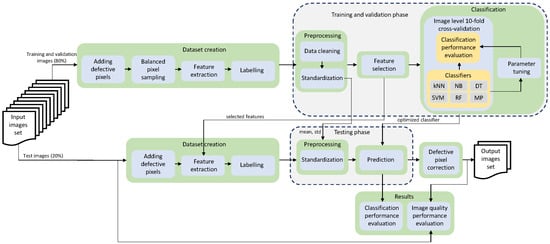
Figure 1 illustrates the methodology employed in this study, from dataset creation to the evaluation of classification and image quality metrics. The dataset is generated independently for each image by synthetically introducing defective pixels, selecting an equal number of non-defective pixels, extracting features, and assigning labels. The image set is partitioned at the image level, with 80% of the images used for training and validation and the remaining 20% reserved for testing. During the training and validation phase, preprocessing, feature selection, image-level cross-validation, and hyperparameter tuning are performed to obtain an optimized classifier. In the testing phase, the selected features and standardization parameters derived from the training set are applied to predict defective pixels, followed by correction using a median filter. Finally, the results are evaluated using both classification and image quality metrics.

Figure 1. Diagram of the proposed methodology. The dataset is generated independently for each image by synthetically introducing defective pixels, selecting an equal number of non-defective pixels, extracting features, and assigning labels. The image set is partitioned at the image level into 80% for training and validation and 20% for testing. The training phase includes preprocessing, feature selection, cross-validation, and hyperparameter tuning to obtain an optimized classifier. During testing, the selected features and standardization parameters from the training set are applied for defective pixel prediction, correction using a median filter, and performance evaluation.

3.1. Image Dataset

The experiments were performed using the TAMPERE17 dataset [34], a freely available and widely used resource within the research community. It is commonly employed for evaluating digital image processing methods, including image denoising [41,42], blind noise estimation [43,44], and lossy compression [45,46]. The dataset consists of 300 grayscale images, each with a resolution of $512\times 512$ pixels, carefully selected to represent diverse visual characteristics, including highly textured scenes, extensive homogeneous regions, and self-similar textures. The use of grayscale images simplifies feature extraction and focuses the evaluation on intensity-based anomalies, which are the primary target of defective pixel detection. Synthetic defective pixels are subsequently introduced to generate labeled datasets for training, validation, and testing.

To simulate defective pixels, 0.5% of the pixels in each image were modified, generating both dead and hot pixels. Dead pixels were assigned intensity values within the lowest 5% of the full dynamic range, while hot pixels were assigned values within the highest 5% of the range. These settings are consistent with the evaluation criteria used in previous studies [12,14,19,20,22,23].

For each image, defective pixel locations were randomly selected without repetition to ensure unique coordinates. The generated defects were equally divided between dead and hot pixels, and their intensity values were sampled from a uniform distribution within the specified ranges. Stuck pixels were intentionally excluded from this study because their detection generally requires temporal or multi-frame analysis, whereas the proposed methodology is based exclusively on spatial features extracted from a single image. A fixed random seed was used to ensure reproducibility of the defect generation process, while independent random realizations were generated for each image to avoid identical defect patterns across the dataset.

3.2. Image Feature Extraction

After constructing the image dataset, the next step involves generating the feature dataset by extracting local descriptors from pixel neighborhoods. Each image is processed using a sliding window from which local features are extracted. To evaluate the influence of neighborhood size on classification performance, feature extraction was performed using neighborhood windows of $3\times 3$, $5\times 5$, and $7\times 7$ pixels. For each window, 10 features were extracted. Each window was subsequently associated with a label according to the state of its central pixel, classifying it as defective or non-defective. Four of these features were calculated directly from the pixel intensities within the window, capturing local intensity variations and spatial relationships among neighboring pixels. The remaining features were computed using the GLCM calculated over the corresponding neighborhood window to characterize more complex textural patterns.

• Feature_1: The absolute intensity difference between the central pixel and the mean intensity of its surrounding neighbors within the window.
• Feature_2: The standard deviation of pixel intensities within the window, including the central pixel. This metric quantifies the local dispersion of intensity values, reflecting the variability of pixel intensities within the neighborhood.
• Feature_3: The normalized intensity range within the window, calculated as the difference between the maximum and minimum pixel values, divided by the full dynamic range of pixel intensities.
• Feature_4: The kurtosis of pixel intensities within the window, used to quantify the tailedness or sharpness of the local intensity distribution. This feature helps highlight regions with extreme intensity deviations.
• Feature_5: The contrast derived from the GLCM, measuring the local intensity variation between pixel pairs. Higher values indicate greater differences between neighboring intensities.
• Feature_6: The correlation from the GLCM, which assesses the linear relationship between a pixel and its neighbors, reflecting the degree of structural similarity in the window.
• Feature_7: The energy computed from the GLCM, indicating the textural uniformity of the local region. Higher energy suggests homogeneous areas, while lower values may signal textural irregularities or defects.
• Feature_8: The entropy from the GLCM, measuring the randomness or complexity of pixel intensity relationships. Higher entropy denotes greater texture complexity, whereas lower entropy reflects more regular patterns.
• Feature_9: The dissimilarity from the GLCM, representing the mean absolute difference between neighboring pixel intensities. Larger values correspond to greater local contrast, while smaller values imply smoother textures.
• Feature_10: The homogeneity from the GLCM, indicating how close GLCM elements are to its diagonal. Higher homogeneity values imply similar neighboring intensities, typical of smooth regions, while lower values reveal abrupt textural changes or defects.

The GLCM features were computed using a fixed set of parameters. Co-occurrence matrices were calculated considering 256 gray levels, a pixel distance of 1, and four directions ($0^{\circ }$, ${45}^{\circ }$, ${90}^{\circ }$, and ${135}^{\circ }$). The resulting GLCMs were normalized and made symmetric. The final feature values were obtained by averaging the corresponding GLCM features across all directions. The resulting feature set was subsequently analyzed to identify the most informative descriptors for defective pixel classification.

3.3. Feature Dataset Preprocessing

The feature dataset preprocessing constitutes the first stage of the training and validation process and includes dataset partitioning, data cleaning, and feature standardization. In this work, each instance corresponds to a central pixel whose features are extracted from a neighborhood window of size $3\times 3$, $5\times 5$, or $7\times 7$, depending on the evaluated configuration, allowing the problem to be formulated as a pixel-level classification task.

To ensure a reliable evaluation protocol and avoid information leakage, the dataset partitioning is performed at the image level prior to feature extraction. Specifically, the 300 images are divided into 240 images (80%) for training and validation and 60 images (20%) for testing. Feature extraction using the sliding window approach is then applied independently within each set, ensuring that all pixel-window instances derived from a given image belong exclusively to either the training or testing set. This prevents spatially correlated samples from the same image from appearing in both sets. Although overlapping windows introduce correlation among neighboring pixel-level instances, this does not lead to information leakage, as no windows from the same image are shared across sets. The use of overlapping windows is necessary to preserve pixel-level resolution and ensure full spatial coverage, particularly given the low proportion of defective pixels in the dataset.

After feature extraction, preprocessing steps are applied independently to the training and testing subsets. Feature standardization is performed using the mean and standard deviation computed from the training subset, and the resulting parameters are subsequently applied to the testing subset to avoid information leakage. Rows containing invalid values are removed from both subsets. After feature extraction, the complete dataset initially contained a substantially larger number of non-defective pixel-window instances than defective ones due to the low proportion of defective pixels introduced in the images. To address this class imbalance, an undersampling strategy was applied by randomly selecting non-defective samples for each image, resulting in a balanced dataset. After preprocessing and undersampling, the training and validation subset contained 309,482 defective pixel-window instances (50.02%) and 309,243 non-defective pixel-window instances (49.98%), while the independent testing subset contained 77,400 defective pixel-window instances (50.00%) and 77,387 non-defective pixel-window instances (50.00%).

3.4. Feature Selection

The initial feature dataset contains 10 distinct features extracted from local pixel neighborhoods. To identify the most informative descriptors for defective pixel classification, a filter-based feature selection approach was employed using various statistical estimators, including correlation-based metrics, group difference tests, and information-theoretic measures such as Pearson correlation, analysis of variance (ANOVA), chi-squared test, information gain, Gini index, and gain ratio. As shown in Table 1, each estimator was applied to evaluate the relationship between individual features and the target variable.

Table 1. Statistical evaluation of the extracted features using filter-based feature selection methods.

Features	Pearson	ANOVA	Chi2	Information Gain	Gini	Gain Ratio
Feature_1	0.80	91,855.64	9488.15	0.52	0.60	0.28
Feature_2	0.43	11,939.49	996.93	0.12	0.04	0.06
Feature_3	0.55	23,106.43	3185.95	0.18	0.05	0.07
Feature_4	0.47	15,112.94	4654.71	0.17	0.10	0.10
Feature_5	0.51	18,444.67	1672.84	0.21	0.09	0.17
Feature_6	−0.48	15,589.11	656.54	0.15	0.03	0.08
Feature_7	−0.04	91.97	13.22	0.01	0.01	0.01
Feature_8	0.05	125.10	1.08	0.01	0.01	0.06
Feature_9	0.46	14,107.13	1216.28	0.14	0.03	0.08
Feature_10	−0.05	166.48	24.33	0.05	0.02	0.03

A cross-voting strategy was applied to identify the most relevant features based on the rankings provided by different statistical estimators. For each estimator, the features were ranked according to their numerical scores, and points were assigned proportionally to their ranking positions, with the highest-ranked feature receiving the maximum score. The cumulative scores obtained across all estimators were then used to determine the final subset of selected features. As shown in Table 1, Feature_7, Feature_8, and Feature_10 consistently received lower scores than the remaining descriptors and were therefore excluded. Consequently, Feature_1, Feature_2, Feature_3, Feature_4, Feature_5, Feature_6, and Feature_9 were retained, resulting in a final set of seven features used for classifier training, validation, and testing.

It is worth noting that Feature_1 consistently achieved the highest score across all evaluated filter methods. This result indicates that the local intensity deviation between the central pixel and its neighborhood is the most informative descriptor for distinguishing defective and non-defective pixels in the evaluated dataset. The remaining selected features provide complementary statistical and texture information that contributes to classifier performance.

The proposed cross-voting strategy provides a robust mechanism for integrating information from multiple estimators without requiring scale normalization or arbitrary threshold selection.

3.5. Classification Algorithms for Defective Pixel Detection

All classifiers were trained and evaluated using the seven selected features identified in Section 3.4. The evaluated classifiers for defective pixel classification included k-Nearest Neighbors, Naïve Bayes, Decision Tree, Random Forest, Support Vector Machine, and Multilayer Perceptron. Model selection and hyperparameter tuning were performed using exhaustive search procedures combined with 10-fold GroupKFold cross-validation on the training subset, ensuring that all instances derived from a given image remained within the same fold. For each classifier, multiple candidate hyperparameter configurations were evaluated, and the configuration yielding the highest average phi coefficient across the validation folds was selected. The cross-validation procedure was conducted at the image level, consistent with the dataset partitioning strategy described in Section 3.3. The hyperparameter search spaces, parameter settings, and selected configurations for each algorithm are summarized in Table 2, which reports the search spaces considered during hyperparameter optimization together with the final configurations selected through the cross-validation tuning process.

Table 2. Hyperparameter search spaces, parameter settings, and selected configurations of the supervised machine learning algorithms used in the study.

Algorithm	Parameter	Search Space/Setting	Selected Value
kNN	Number of neighbors (k)	$\{1,\dots ,10\}$	7
	Distance metric	Euclidean	Euclidean
	Weight	Uniform	Uniform
Naïve Bayes	Variant	GaussianNB	GaussianNB
	Variance smoothing	${10}^{-9}$	${10}^{-9}$
Decision Tree	Criterion	{Gini, Entropy}	Gini
	Minimum samples per leaf	{1, 2, 5}	5
	Minimum samples for split	{2, 5, 10}	2
	Maximum depth	{None, 5, 10}	10
Random Forest	Number of trees	{5, 10, 20}	10
	Criterion	{Gini, Entropy}	Gini
	Maximum tree depth	Unlimited	Unlimited
SVM (RBF)	Kernel	RBF	RBF
	Regularization parameter (C)	{0.1, 1, 10}	10
	Kernel coefficient ($\gamma$)	{0.001, 0.01, 0.1, 1}	1
	Iteration limit	Unlimited	Unlimited
SVM (Polynomial)	Kernel	Polynomial	Polynomial
	Polynomial degree	{1, 2}	2
	Regularization parameter (C)	{0.1, 1, 10}	10
	Kernel coefficient ($\gamma$)	{0.001, 0.01, 0.1, 1}	1
	Iteration limit	Unlimited	Unlimited
Multilayer Perceptron	Hidden layer sizes	{(64), (64, 32), (128, 64)}	(64, 32)
	Activation	{tanh, ReLU}	ReLU
	Solver	{Adam, SGD}	Adam
	Regularization parameter ($\alpha$)	{0.0001, 0.001, 0.01}	0.001
	Iteration limit	200	200

Among the six evaluated algorithms, the kNN and Naïve Bayes classifiers were configured as follows: The kNN model was configured with $k=7$, using the Euclidean distance metric and uniform weighting. In this setup, each pixel is classified based on a majority vote among its seven nearest neighbors in the feature space, with all neighbors contributing equally to the classification. The Naïve Bayes classifier was configured using the GaussianNB variant with a variance smoothing parameter of $1\times {10}^{-9}$, which helps stabilize computations in the presence of features with very low variance. This probabilistic model assumes that features are Gaussian-distributed and conditionally independent given the class label.

The Decision Tree was configured using the Gini impurity criterion, a maximum depth of 10, a minimum of five instances per leaf node, and a minimum of two instances in internal nodes. These constraints aim to control overfitting while maintaining model interpretability. The Random Forest model comprised 10 decision trees, also using the Gini criterion, with no restrictions on tree depth. This allowed each tree to grow fully and independently, promoting diversity among the trees and improving generalization through ensemble averaging.

We evaluated the SVM classifier using two configurations. The first configuration used a Radial Basis Function (RBF) kernel with $C=10$, $\gamma =1$, and no limit on training iterations. This kernel enables the model to learn non-linear decision boundaries by mapping inputs into a higher-dimensional feature space. The second configuration used a Polynomial kernel of degree 2, using the same values of the regularization parameter C and the kernel parameter $\gamma$. This configuration enables the model to capture quadratic feature interactions, providing a trade-off between linear and more complex non-linear mappings with moderate computational cost.

Finally, the Multilayer Perceptron was configured with two hidden layers containing 64 and 32 neurons, respectively. The activation function was ReLU, introducing non-linearity to capture complex feature relationships. The model was trained using the Adam optimizer, with a regularization parameter of $\alpha =0.001$ to reduce overfitting, and the maximum number of training iterations was set to 200.

4. Results

We evaluated six supervised machine learning classifiers for defective pixel classification: k-Nearest Neighbors, Naïve Bayes, Decision Tree, Random Forest, Support Vector Machine, and Multilayer Perceptron. Model selection and hyperparameter tuning were performed using 10-fold image-level cross-validation on the training and validation set (80% of the images). The performance metrics were obtained from the independent test set (20% of the images), which was not used during model training or hyperparameter tuning. The evaluated metrics include specificity, recall, precision, and the phi coefficient, which are defined as follows:

$$\begin{array}{ccc}\hfill specificity& =& {\displaystyle \frac{TN}{TN+FP}}\hfill \end{array}$$

(1)

$$\begin{array}{ccc}\hfill recall& =& {\displaystyle \frac{TP}{TP+FN}}\hfill \end{array}$$

(2)

$$\begin{array}{ccc}\hfill precision& =& {\displaystyle \frac{TP}{TP+FP}}\hfill \end{array}$$

(3)

$$\begin{array}{ccc}\hfill phicoefficient& =& {\displaystyle \frac{TP\times TN-FP\times FN}{\sqrt[ ]{(TP+FP)\times (TP+FN)\times (TN+FP)\times (TN+FN)}}},\hfill \end{array}$$

(4)

where $TP$ denotes the number of true positive defective pixels correctly identified by the algorithm, $TN$ represents the number of true negatives (non-defective pixels correctly classified), $FP$ corresponds to false positives (non-defective pixels incorrectly classified as defective), and $FN$ refers to false negatives (defective pixels missed by the algorithm). Specificity indicates the proportion of non-defective pixels correctly identified. Recall measures the proportion of actual defective pixels that were correctly detected. Precision expresses the proportion of predicted defective pixels that are truly defective. Finally, the phi coefficient is a special case of the Pearson correlation coefficient that quantifies the degree of association between predicted and actual classifications, capturing the balance between correctly and incorrectly classified pixels.

Table 3 presents a comparison of the performance metrics for the six supervised machine learning classifiers applied to defective pixel classification, using neighborhood windows of 3 × 3, 5 × 5, and 7 × 7, evaluated on the independent test set. The results show that the neighborhood size has a noticeable impact on classification performance. The highest phi coefficient (98.08%) was achieved by the SVM classifier with an RBF kernel using a 3 × 3 feature extraction window, together with a specificity of 99.00%, a recall of 99.00%, and a precision of 99.02%. In general, the 3 × 3 window produced the best results across most classifiers, whereas the 7 × 7 window resulted in lower performance. These findings suggest that defective pixels are primarily characterized by highly local intensity variations and that larger neighborhoods may introduce additional contextual information that is less discriminative for the classification task.

Table 3. Performance metrics of the supervised machine learning classifiers for defective pixel classification obtained using different neighborhood window sizes (3 × 3, 5 × 5, and 7 × 7) for feature extraction. Results are reported on the independent test set in terms of specificity, recall, precision, and the phi coefficient.

Window Size	Classifier	Specificity (%)	Recall (%)	Precision (%)	Phi Coefficient (%)
3 × 3	kNN (k = 7)	98.84	97.75	98.66	96.59
	Decision Tree	97.66	97.73	97.72	95.40
	Random Forest	98.81	98.13	98.84	96.93
	Naïve Bayes	94.09	91.90	94.11	86.07
	SVM (RBF)	99.00	99.00	99.02	98.08
	SVM (POLY)	94.46	78.85	93.60	74.10
	Multilayer Perceptron	99.09	97.96	99.01	97.04
5 × 5	kNN (k = 7)	99.01	97.17	98.99	96.20
	Naïve Bayes	88.10	90.03	88.33	78.14
	Decision Tree	97.39	97.41	97.39	94.80
	Random Forest	98.91	97.77	98.90	96.68
	SVM (RBF)	99.11	97.75	99.09	96.86
	SVM (POLY)	95.98	77.02	95.04	74.35
	Multilayer Perceptron	99.02	97.88	99.01	96.90
7 × 7	kNN (k = 7)	98.51	96.96	98.49	95.49
	Decision Tree	96.74	96.90	96.74	93.65
	Random Forest	98.49	97.44	98.48	95.94
	Naïve Bayes	85.28	90.91	85.96	75.46
	SVM (RBF)	98.69	97.33	98.67	95.64
	SVM (POLY)	93.41	70.70	91.48	65.83
	Multilayer Perceptron	98.56	97.61	98.54	96.18

Among the evaluated classifiers, SVM (RBF) consistently achieved the highest performance levels across the different neighborhood sizes. In contrast, the polynomial-kernel SVM exhibited considerably lower performance, particularly in terms of recall and phi coefficient. This result suggests that the selected feature set is better represented by the flexible non-linear decision boundary provided by the RBF kernel than by polynomial transformations. Multilayer Perceptron also achieved highly competitive performance across all evaluated window sizes and was statistically comparable to SVM (RBF), although the latter consistently achieved the highest observed classification performance. The consistently higher observed performance of SVM (RBF) is particularly important in applications where minimizing false positives and false negatives contributes to more accurate defective pixel localization and improved image quality in subsequent correction stages.

Although classification performance varied with the neighborhood size, the average feature extraction time remained approximately constant for all evaluated configurations, with values close to 40 s per image. These measurements were obtained on a workstation equipped with an AMD Ryzen 7 8845HS processor and 16 GB of RAM, using the complete training dataset composed of 240 images. This behavior indicates that the computational cost is largely dominated by the computation of the GLCM-based descriptors rather than by the number of pixels contained in the neighborhood window. Therefore, while the neighborhood size influences the discriminative power of the extracted features, its impact on the overall feature extraction time was negligible in the evaluated implementation.

To assess whether the observed differences among classifiers were statistically significant, a Friedman test was performed using the phi coefficient values obtained from the 10-fold GroupKFold cross-validation for the best-performing 3 × 3 feature extraction window. The test revealed statistically significant differences among the evaluated classifiers ($p<0.001$). A subsequent Nemenyi post-hoc analysis showed that Multilayer Perceptron and SVM (RBF), which achieved the two best average rankings (1.8 and 1.9, respectively), did not differ significantly from each other. These results indicate that both classifiers provide statistically comparable performance under the evaluated experimental conditions, while SVM (RBF) with a 3 × 3 feature extraction window achieved the highest observed phi coefficient among all evaluated configurations.

Table 4 summarizes the computational cost associated with hyperparameter tuning, model training, and testing for each evaluated classifier. Considerable differences were observed among the evaluated methods. Naïve Bayes, kNN, Decision Tree, and Random Forest exhibited relatively low computational requirements, requiring less than 237 s for hyperparameter tuning and less than 4 s for model training. In contrast, the kernel-based SVM classifiers were substantially more computationally demanding. SVM (RBF), which achieved the highest observed $\varphi$ coefficient, required 13,140.81 s for hyperparameter tuning and 1243.36 s for model training, whereas SVM (Polynomial) required 32,944.97 s and 23,179.30 s, respectively. Although no statistically significant differences were observed between Multilayer Perceptron and SVM (RBF), the former required considerably lower computational effort, with a hyperparameter tuning time of 3286.68 s and a training time of only 65.69 s. These results indicate that, among the evaluated classifiers, SVM (RBF) achieved the highest observed classification performance. Although no statistically significant differences were found with Multilayer Perceptron, the latter offers an excellent trade-off between predictive performance and computational efficiency.

Table 4. Computational cost of the evaluated supervised machine learning classifiers. Hyperparameter tuning time, training time, and testing time measured on the workstation described in the text using the optimized configurations reported in Table 2.

Classifier	Hyperparameter	Training	Testing
	Tuning Time (s)	Time (s)	Time (s)
kNN	41.79	0.69	2.97
Naïve Bayes	0.00	0.03	0.01
Decision Tree	236.19	2.86	0.01
Random Forest	83.71	3.43	0.04
SVM (RBF)	13,140.81	1243.36	149.88
SVM (Polynomial)	32,944.97	23,179.30	148.52
Multilayer Perceptron	3286.68	65.69	0.15

Table 5 presents a comparative analysis between the best-performing configuration identified in Table 3, namely SVM with an RBF kernel and a 3 × 3 feature extraction window, and several state-of-the-art methods for defective pixel classification. The reported metrics for the state-of-the-art methods were extracted from their original publications, while the results for SVM (RBF) were obtained using the dataset employed in this study.

Table 5. Performance comparison between the best-performing configuration identified in this study (SVM with RBF kernel and a 3 × 3 feature extraction window) and state-of-the-art defective pixel detection methods. Metrics include specificity, recall, precision, and phi coefficient. Missing values are indicated with a dash.

Algorithms	Specificity (%)	Recall (%)	Precision (%)	Phi Coefficient (%)
Chan [19]	90.06	96.13	8.88	27.59
Yongji [23]	93.93	84.68	12.11	31.21
Cho [20]	99.37	96.54	92.68	77.31
Tchendjou2018a [22]	99.80	95.59	84.91	89.74
Tchendjou2018b [22]	99.79	95.68	84.35	89.49
Tchendjou2020 [12]	99.92	95.14	92.77	93.85
López-Portilla [14]	99.91	94.70	91.22	92.84
Çelik [31]	-	80.00	99.00	-
Çelik [13]	-	97.80	97.00	-
Ferreira [32]	-	92.10	88.80	-
SVM (RBF)	99.00	99.00	99.02	98.08

The proposed SVM (RBF) classifier achieved highly competitive performance across all reported metrics. Compared with the reviewed state-of-the-art methods, it obtained the highest phi coefficient (98.08%), indicating a superior balance between correctly and incorrectly classified pixels. In addition, the classifier achieved a specificity of 99.00%, a recall of 99.00%, and a precision of 99.02%, outperforming most of the reported approaches. However, it is important to note that the reported results correspond to different datasets and experimental conditions; therefore, the comparison should be interpreted as indicative rather than as a direct benchmark. Nevertheless, these findings support the effectiveness of the proposed methodology for defective pixel classification.

In addition to the strong performance achieved by SVM (RBF), the other machine learning algorithms evaluated in Table 3, particularly Multilayer Perceptron, Random Forest, and Decision Tree, also showed competitive performance across the evaluated metrics. These results indicate that several supervised learning algorithms are suitable for defective pixel classification under the evaluated experimental conditions. However, the observed differences in classification performance indicate that the choice of classifier can significantly influence the final detection accuracy, with SVM (RBF) providing the best overall results among the evaluated approaches.

Once defective pixels were detected, they were corrected using a median filter applied to their eight neighboring pixels. The median filter was employed solely as a simple post-processing step to assess the impact of detection accuracy on image quality, rather than as an optimized correction strategy. A quantitative evaluation of the results was then performed using two widely used image quality metrics: Peak Signal-to-Noise Ratio (PSNR) and Structural Similarity Index Measure (SSIM) [6]. In all cases, subscript R denotes the original defect-free (reference) images, while subscript 0 corresponds to the reconstructed images obtained after defective pixel detection and median filter correction (output images). The PSNR metric is determined using the maximum possible pixel intensity and the Mean Squared Error (MSE), as described in the following equation:

$$PSNR=10\times log{\displaystyle \frac{{\left(2^n-1\right)}^2}{MSE}},$$

(5)

where n is the number of bits used to encode the intensity value of a pixel and $MSE$ is calculated as follows:

$$MSE={\displaystyle \frac{1}{M\times N}}{\displaystyle \sum _{i=1}^M}{\displaystyle \sum _{j=1}^N}{\left(X_0(i,j)-X_R(i,j)\right)}^2,$$

(6)

where $X_R$ is the reference image, $X_0$ is the output image, and M and N are the dimensions of the images.

The SSIM is a widely used metric for evaluating image quality, as it quantifies similarity between images based on luminance, contrast, and structural information. It is computed locally over small windows and then averaged to obtain a global similarity measure, as shown in the following equation:

$$SSIM={\displaystyle \frac{(2{\mu }_0{\mu }_R+C_1)(2{\sigma }_{0,R}+C_2)}{({\mu }_0^2+{\mu }_R^2+C_1)({\sigma }_0^2+{\sigma }_R^2+C_2)}},$$

(7)

where $C_1$ and $C_2$ are small constants that stabilize the computation; ${\mu }_0$ and ${\mu }_R$ represent the local mean intensities of the output and reference images, respectively; ${\sigma }_0$ and ${\sigma }_R$ are the corresponding local standard deviations; and ${\sigma }_{0,R}$ denotes the local cross-covariance between the output and reference images, computed over a local window.

Table 6 presents a quantitative comparison of image quality after applying various algorithms for defective pixel detection followed by median filter correction. PSNR and SSIM are used as evaluation metrics. In addition to state-of-the-art methods, a baseline based solely on a $3\times 3$ median filter applied to the entire image is included to assess the benefit of incorporating a prior defective pixel detection stage. The results show that applying only the median filter yields relatively low performance (PSNR: 33.07 dB, SSIM: 94.60%), indicating that indiscriminate filtering can degrade image quality. In contrast, combining defective pixel detection with median filter correction substantially improves the results. The best-performing configuration identified in this study, namely SVM (RBF) with a $3\times 3$ feature extraction window, achieved a PSNR of 40.96 dB and an SSIM of 98.68%, demonstrating that more accurate defective pixel detection leads to improved reconstructed image quality.

Table 6. Comparison of image quality metrics with state-of-the-art defective pixel correction methods.

Algorithms	PSNR (dB)	SSIM (%)
Chan [19]	32.19	88.23
Yongji [23]	32.02	90.10
Cho [20]	32.27	94.54
Tchendjou2018a [22]	41.05	99.43
Tchendjou2020 [12]	40.93	99.41
López-Portilla [14]	47.57	99.84
Median filter only (3 × 3)	33.07	94.60
SVM (RBF) + median filter	40.96	98.68

Although these results do not surpass the best-performing state-of-the-art methods, such as López-Portilla [14] (PSNR: 47.57 dB, SSIM: 99.84%) or Tchendjou2020 [12], they remain competitive and confirm the effectiveness of supervised machine learning for defective pixel detection. In particular, the substantial improvement over the baseline median filtering approach highlights the importance of accurate defective pixel identification prior to correction, suggesting that detection quality has a direct impact on image fidelity preservation. These findings further support the use of SVM-based defective pixel detection combined with a simple median filter correction stage, even without employing a dedicated image restoration algorithm.

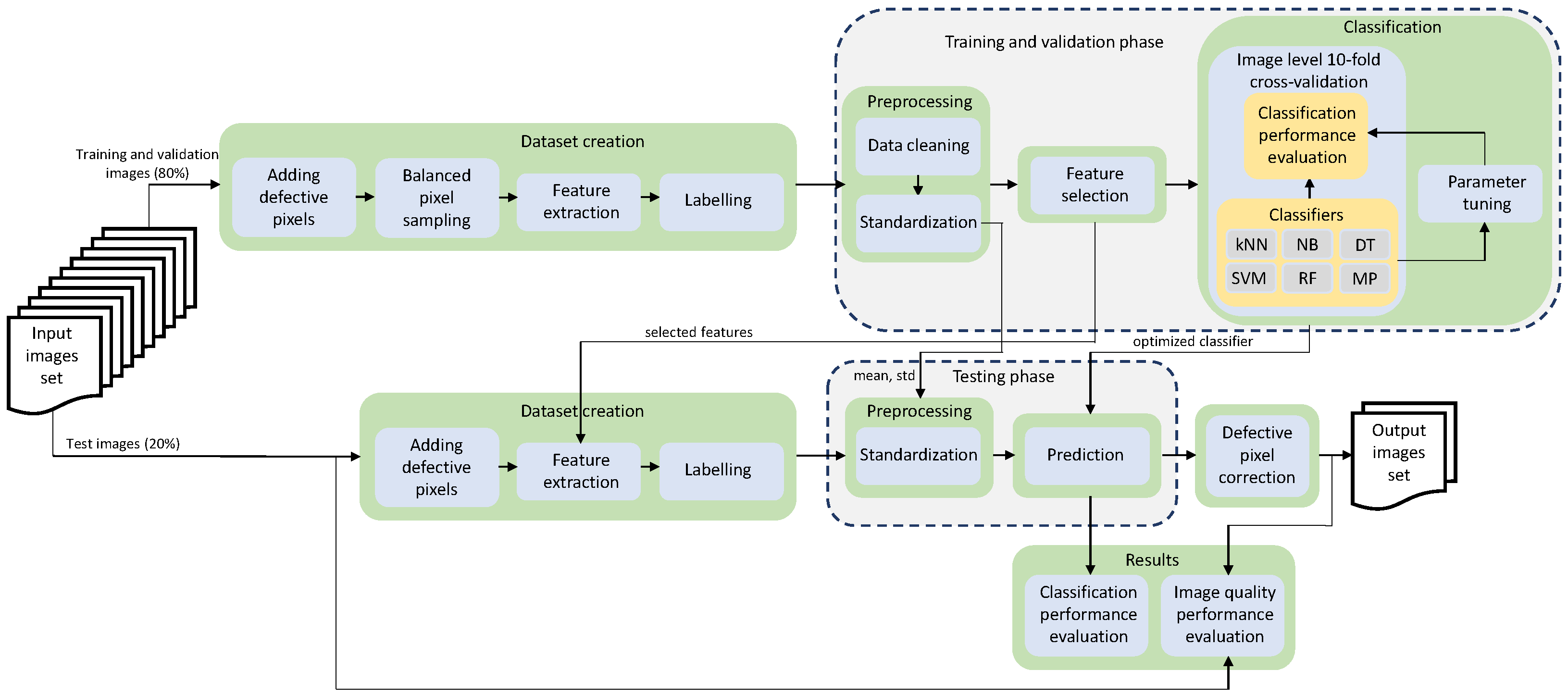
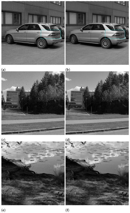
Figure 2a,c,e display sample images from the TAMPERE17 dataset [34] that were artificially corrupted by randomly introducing defective pixels, affecting 0.5% of the total pixels in each image. Dead pixels were randomly initialized with values within the lowest 5% of the full dynamic range, while hot pixels were assigned values within the highest 5%. In contrast, Figure 2b,d,f show the corresponding corrected images obtained after applying the SVM (RBF) detection algorithm followed by median filtering. A visual inspection of the results reveals that most defective pixels were successfully detected and corrected, resulting in a noticeable improvement in overall image quality. These results provide visual evidence of the effectiveness of the proposed defective pixel detection approach and illustrate the impact of accurate detection on subsequent image correction.

Figure 2. Defective pixel processing visualization using the TAMPERE17 dataset [34]. (a,c,e) Original images with 0.5% randomly added defective pixels. (b,d,f) Results obtained with SVM (RBF) detection followed by median filter correction.

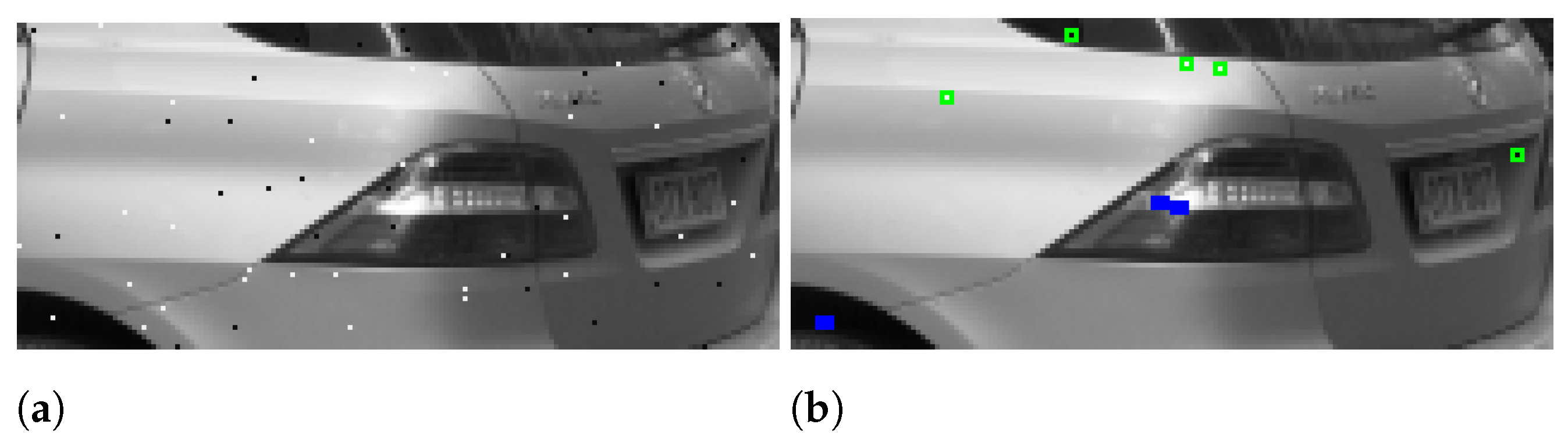
Figure 3 presents a zoomed-in view of the $75\times 150$-pixel region highlighted in cyan in Figure 2a,b. Figure 3a shows more clearly the randomly added dead and hot pixels, which represent 0.5% of the total pixels in the image. Figure 3b illustrates the result of applying the SVM (RBF) algorithm for defective pixel detection, followed by median filter correction. Pixels outlined in blue correspond to false positives, while those outlined in green indicate false negatives. Of the 67 defective pixels present in Figure 3a, the SVM (RBF) algorithm correctly detected 62, misclassifying five defective pixels as non-defective (false negatives). Conversely, six non-defective pixels were incorrectly classified as defective (false positives). As observed in Figure 3, all false positives and false negatives occur in regions where dead pixels appear in very dark backgrounds and hot pixels in very bright backgrounds. In both cases, the visual quality of the corrected image is not significantly affected, suggesting that some classification errors have limited perceptual impact on the final reconstructed image.

Figure 3. Zoomed-in region from a TAMPERE17 dataset image, illustrating examples of false positives and false negatives. (a) Original image with 0.5% of randomly added defective pixels. (b) Result of SVM (RBF)-based detection and median filter correction, highlighting false positive pixels (blue frames) and false negative pixels (green frames).

5. Conclusions

In this paper, we addressed the problem of defective pixel detection in CMOS Image Sensors (CIS) by evaluating the performance of several supervised machine learning algorithms. A total of 300 grayscale images of size $512\times 512$ pixels from the TAMPERE17 dataset [34], artificially degraded with dead and hot pixels, were used to train and evaluate the models. The assessed algorithms included k-Nearest Neighbors, Naïve Bayes, Decision Tree, Random Forest, Support Vector Machine, and Multilayer Perceptron. A sensitivity analysis was also conducted using feature extraction windows of $3\times 3$, $5\times 5$, and $7\times 7$ pixels. Based on specificity, recall, precision, and phi coefficient, the best overall performance was achieved by an SVM classifier with an RBF kernel using a $3\times 3$ feature extraction window, reaching a phi coefficient of 98.08%, together with a specificity of 99.00%, a recall of 99.00%, and a precision of 99.02%. The best-performing configuration also achieved a PSNR of 40.96 dB and an SSIM of 98.68% after median filter correction, demonstrating that improved defective pixel detection translated into improved reconstructed image quality. Although this configuration achieved the highest observed classification performance, no statistically significant differences were found with Multilayer Perceptron under the evaluated experimental conditions.

The use of local statistical and texture-based features extracted from pixel neighborhoods proved effective for defective pixel detection, enabling supervised learning classifiers to accurately distinguish between defective and non-defective pixels even in images with very low defect rates. The sensitivity analysis further revealed that smaller neighborhoods provide more discriminative information, suggesting that defective pixels are primarily characterized by highly local intensity variations. The results also indicate that supervised learning provides a flexible and reproducible framework for defective pixel detection, and the reported findings may serve as reference benchmarks for future studies.

A limitation of this study is that the dataset was synthetically generated, where defective pixels are introduced under controlled conditions. Although this allows systematic and reproducible evaluation, it may not fully capture the complexity, temporal behavior, and variability of real defective pixels in CMOS image sensors. Although the proposed methodology demonstrated strong performance under the evaluated experimental conditions, further validation using real defective pixel datasets is necessary to assess its applicability to real CMOS imaging systems. Furthermore, the correction stage relies on a simple median filter used only to assess the impact of detection accuracy on image quality, rather than as an optimized restoration strategy.

Future research should validate the proposed approach using real sensor data, more diverse defect patterns, and advanced correction methods. Future studies could also investigate replacing the simple median filter employed in this work with more advanced image restoration and denoising frameworks, such as detail-retaining convolutional neural networks, support-denoiser-driven restoration frameworks, deep-denoising-prior-based image restoration techniques, and denoiser-guided image deconvolution methods, which could further improve reconstructed image quality while preserving fine image structures [47,48,49,50]. Moreover, future studies could compare the proposed handcrafted-feature-based framework with modern deep learning approaches for defective pixel detection to better assess the trade-off between classification performance, computational cost, and suitability for deployment in resource-constrained imaging systems. Another promising direction is the extension of the proposed framework toward multi-class defective pixel classification. In particular, incorporating additional defect categories such as stuck pixels could enhance the practical value of the method for image sensor diagnostics, although this would require the inclusion of temporal or multi-frame information beyond the single-frame spatial analysis considered in this work. Furthermore, the implementation of high-performing models such as SVM (RBF) on embedded and sensor-level hardware platforms represents an attractive research direction toward greater portability, lower power consumption, and reduced hardware requirements. Such implementations could enable real-time defective pixel detection in resource-constrained imaging systems and facilitate integration into practical CMOS image sensor applications, including industrial vision, surveillance, and IoT devices.

References

- Radhakrishna, M.; Govindh, M.V.; Veni, P.K. A review on image processing sensor. J. Phys. Conf. Ser. 2021, 1714, 012055. [Google Scholar] [CrossRef] [Scilit]
- Sukhavasi, S.B.; Sukhavasi, S.B.; Elleithy, K.; Abuzneid, S.; Elleithy, A. CMOS Image Sensors in Surveillance System Applications. Sensors 2021, 21, 488. [Google Scholar] [CrossRef] [Scilit] [PubMed]
- Durini, D. High Performance Silicon Imaging: Fundamentals and Applications of CMOS and CCD Sensors; Woodhead Publishing: Cambridge, UK, 2019. [Google Scholar] [CrossRef] [Scilit]
- Liao, F.; Zhou, F.; Chai, Y. Neuromorphic vision sensors: Principle, progress and perspectives. J. Semicond. 2021, 42, 013105. [Google Scholar] [CrossRef] [Scilit]
- Dwik, S.; Lordwin Cecil Prabhaker, M. Survey on energy harvesting CMOS sensor based digital camera. Opt. Mem. Neural Netw. 2022, 31, 97–106. [Google Scholar] [CrossRef] [Scilit]
- Vigil, B.M.L.P.; Valenzuela, W.; Zarkesh-Ha, P.; Figueroa, M. On-chip kernel-based spatial filter for CMOS image sensor. Comput. Electr. Eng. 2025, 123, 110218. [Google Scholar] [CrossRef] [Scilit]
- Park, M.J.; Kim, H.J. A Real-Time Edge-Detection CMOS Image Sensor for Machine Vision Applications. IEEE Sens. J. 2023, 23, 9254–9261. [Google Scholar] [CrossRef] [Scilit]
- Takayanagi, I.; Kuroda, R. HDR CMOS Image Sensors for Automotive Applications. IEEE Trans. Electron. Devices 2022, 69, 2815–2823. [Google Scholar] [CrossRef] [Scilit]
- Yokota, T.; Fukuda, K.; Someya, T. Recent progress of flexible image sensors for biomedical applications. Adv. Mater. 2021, 33, 2004416. [Google Scholar] [CrossRef] [Scilit] [PubMed]
- Riba, J.R. Application of Image Sensors to Detect and Locate Electrical Discharges: A Review. Sensors 2022, 22, 5886. [Google Scholar] [CrossRef] [Scilit] [PubMed]
- Chen, Y.; Kang, J.U.; Zhang, G.; Cao, J.; Xie, Q.; Kwan, C. High-performance concealment of defective pixel clusters in infrared imagers. Appl. Opt. 2020, 59, 4081–4090. [Google Scholar] [CrossRef] [Scilit] [PubMed]
- Tchendjou, G.T.; Simeu, E. Detection, Location and Concealment of Defective Pixels in Image Sensors. IEEE Trans. Emerg. Top. Comput. 2020, 9, 664–679. [Google Scholar] [CrossRef] [Scilit]
- Çelik, A.; Küçükmanisa, A.; Sümer, A.; Çelebi, A.T.; Urhan, O. A real-time defective pixel detection system for LCDs using deep learning based object detectors. J. Intell. Manuf. 2022, 33, 985–994. [Google Scholar] [CrossRef] [Scilit]
- López-Portilla, B.M.; Valenzuela, W.; Zarkesh-Ha, P.; Figueroa, M. A CMOS Image Readout Circuit with On-Chip Defective Pixel Detection and Correction. Sensors 2023, 23, 934. [Google Scholar] [CrossRef] [Scilit] [PubMed]
- Song, X.; Wu, L. Hyperspectral Image Inpainting Based on Robust Spectral Dictionary Learning. Appl. Sci. 2019, 9, 3062. [Google Scholar] [CrossRef] [Scilit]
- Wu, A.; Zhu, J.; Tao, Z.; Mao, C. Automatic inspection and classification for thin-film transistor liquid crystal display surface defects based on particle swarm optimization and one-class support vector machine. Adv. Mech. Eng. 2016, 8, 1687814016677660. [Google Scholar] [CrossRef] [Scilit]
- Chang, Y.C.; Chang, K.H.; Meng, H.M.; Chiu, H.C. A Novel Multicategory Defect Detection Method Based on the Convolutional Neural Network Method for TFT-LCD Panels. Math. Probl. Eng. 2022, 2022, 6505372. [Google Scholar] [CrossRef] [Scilit]
- Lin, Z.H.; Lai, Q.Y.; Li, H.Y. A Machine-Learning Strategy to Detect Mura Defects in a Low-Contrast Image by Piecewise Gamma Correction. Sensors 2024, 24, 1484. [Google Scholar] [CrossRef] [Scilit] [PubMed]
- Chan, C.H. Dead Pixel Real-Time Detection Method for Image. U.S. Patent 7,589,770, 15 September 2009. [Google Scholar]
- Cho, C.Y.; Chen, T.M.; Wang, W.S.; Liu, C.N. Real-time photo sensor dead pixel detection for embedded devices. In Proceedings of the 2011 International Conference on Digital Image Computing: Techniques and Applications; IEEE: Piscataway, NJ, USA, 2011; pp. 164–169. [Google Scholar] [CrossRef] [Scilit]
- El-Yamany, N. Robust Defect Pixel Detection and Correction for Bayer Imaging Systems. Electron. Imaging 2017, 2017, 46–51. [Google Scholar] [CrossRef] [Scilit]
- Tchendjou, G.T.; Simeu, E. Self-healing imager based on detection and conciliation of defective pixels. In Proceedings of the 2018 IEEE 24th International Symposium on On-Line Testing and Robust System Design (IOLTS); IEEE: Piscataway, NJ, USA, 2018; pp. 251–254. [Google Scholar] [CrossRef] [Scilit]
- Yongji, L.; Xiaojun, Y. A Design of Dynamic Defective Pixel Correction for Image Sensor. In Proceedings of the 2020 IEEE International Conference on Artificial Intelligence and Information Systems (ICAIIS); IEEE: Piscataway, NJ, USA, 2020; pp. 713–716. [Google Scholar] [CrossRef] [Scilit]
- Silva, M.O.; Ferreira, D.A.O.; Ouchi, K.Y.; Torres, G.M.; Urtiga Mattos, E.V.; Pereira, A.M.C.; Costa, L.R.; Cavalcante, V.L.G.; Cruz, C.F.; Silva, A.P.; et al. Automated Bright Pixel Detection System on LCD Displays. In Proceedings of the 2021 IEEE International Conference on Consumer Electronics (ICCE); IEEE: Piscataway, NJ, USA, 2021; pp. 1–4. [Google Scholar] [CrossRef] [Scilit]
- Guo, B.; Hu, G.Q.; Yang, G.Y. TFT-LCD spot-type defect detection in module process. Adv. Mater. Res. 2014, 971, 1368–1371. [Google Scholar] [CrossRef] [Scilit]
- Qian, J.; Li, W.; Chen, B.; Qian, J.; Liu, F.; Zhou, X. Sub-Pixel Defect Detection for Super Large LCD Images Using Quadrant Gradient Operator. In Proceedings of the 2018 IEEE 18th International Conference on Communication Technology (ICCT); IEEE: Piscataway, NJ, USA, 2018; pp. 1183–1187. [Google Scholar] [CrossRef] [Scilit]
- Guo, L.; Li, S.; Hu, W.; Wu, J.; Tu, B.; He, W.; Ou, X.; Zhang, G. Sub-Pixel Level Defect Detection Based on Notch Filter and Image Registration. Int. J. Pattern Recognit. Artif. Intell. 2018, 32, 1854016. [Google Scholar] [CrossRef] [Scilit]
- Sümer, A.; Çelık, A.; Küçükmanısa, A.; Taıyapi Çelebı, A.; Urhan, O. Pixel Defect Detection in LCD TV Images using Adaptive Thresholding. In Proceedings of the 2019 27th Signal Processing and Communications Applications Conference (SIU); IEEE: Piscataway, NJ, USA, 2019; pp. 1–4. [Google Scholar] [CrossRef] [Scilit]
- Yang, S.W.; Lin, C.S.; Lin, S.K.; Chiang, H.T. Automatic defect recognition of TFT array process using gray level co-occurrence matrix. Optik 2014, 125, 2671–2676. [Google Scholar] [CrossRef] [Scilit]
- Chu, M.; Gong, R.; Gao, S.; Zhao, J. Steel surface defects recognition based on multi-type statistical features and enhanced twin support vector machine. Chemom. Intell. Lab. Syst. 2017, 171, 140–150. [Google Scholar] [CrossRef] [Scilit]
- Çelik, A.; Sümer, A.; Küçükmanisa, A.; Taşyapı Çelebi, A.; Urhan, O. LCD Pixel defect detection using GLCM features and SVM. In Proceedings of the International Marmara Science and Social Sciences Congress; Kocaeli University: Kocaeli, Turkey, 2018; pp. 853–858. [Google Scholar]
- Ferreira, D.A.; Amoedo, D.A.; Costa, L.R.; Valadão, M.D.; Souza, A.S.; Ouchi, K.Y.; Pereira, A.M.; Torres, G.M.; Silva, M.O.; Cruz, C.F.; et al. Dead Pixel Detection on Liquid Crystal Displays using Random Forest, SVM, and Harris Detector. In Proceedings of the 2020 IEEE International Conference on Consumer Electronics-Taiwan (ICCE-Taiwan); IEEE: Piscataway, NJ, USA, 2020; pp. 1–2. [Google Scholar] [CrossRef] [Scilit]
- Çelik, A.; Küçükmanisa, A.; Sümer, A.; Taşyapi Çelebi, A.; Urhan, O. LCD Pixel Defect Detection using Shallow CNN Based Approach. In Proceedings of the 2021 International Conference on INnovations in Intelligent SysTems and Applications (INISTA); IEEE: Piscataway, NJ, USA, 2021; pp. 1–6. [Google Scholar] [CrossRef] [Scilit]
- Ponomarenko, M.; Gapon, N.; Voronin, V.; Egiazarian, K. Blind estimation of white Gaussian noise variance in highly textured images. In Proceedings of the IS&T International Symposium on Electronic Imaging: Image Processing: Algorithms and Systems XVI; Society for Imaging Science and Technology: Burlingame, CA, USA, 2018; pp. 382-1–382-5. [Google Scholar] [CrossRef] [Scilit]
- Ming, W.; Zhang, S.; Liu, X.; Liu, K.; Yuan, J.; Xie, Z.; Sun, P.; Guo, X. Survey of Mura Defect Detection in Liquid Crystal Displays Based on Machine Vision. Crystals 2021, 11, 1444. [Google Scholar] [CrossRef] [Scilit]
- Chen, P.; Chen, M.; Wang, S.; Song, Y.; Cui, Y.; Chen, Z.; Zhang, Y.; Chen, S.; Mo, X. Real-time defect detection of TFT-LCD displays using a lightweight network architecture. J. Intell. Manuf. 2024, 35, 1337–1352. [Google Scholar] [CrossRef] [Scilit]
- Tchendjou, G.T.; Simeu, E. Defective pixel analysis for image sensor online diagnostic and self-healing. In Proceedings of the 2019 IEEE 37th VLSI Test Symposium (VTS); IEEE: Piscataway, NJ, USA, 2019; pp. 1–6. [Google Scholar] [CrossRef] [Scilit]
- Rahmani, M.C.; Khatir, A.; Azad, M.M.; Kim, H.S.; Firouzi, N.; Kumar, R.; Khatir, S.; Cuong, L.T. Mechanics-based deep learning framework for predicting deflection of functionally graded composite plates using an enhanced whale optimization algorithm. Math. Mech. Solids 2025, 10812865251398866. [Google Scholar] [CrossRef] [Scilit]
- Narayanan, R.; Ganesh, N. A comprehensive review of metaheuristics for hyperparameter optimization in machine learning. In Metaheuristics for Machine Learning: Algorithms and Applications; Wiley: Hoboken, NJ, USA, 2024; pp. 37–72. [Google Scholar] [CrossRef] [Scilit]
- Barrera-García, J.; Cisternas-Caneo, F.; Crawford, B.; Gómez Sánchez, M.; Soto, R. Feature Selection Problem and Metaheuristics: A Systematic Literature Review about Its Formulation, Evaluation and Applications. Biomimetics 2024, 9, 9. [Google Scholar] [CrossRef] [Scilit] [PubMed]
- Bahnemiri, S.G.; Ponomarenko, M.; Egiazarian, K. Learning-Based Noise Component Map Estimation for Image Denoising. IEEE Signal Process. Lett. 2022, 29, 1407–1411. [Google Scholar] [CrossRef] [Scilit]
- Shevkunov, I.; Ponomarenko, M.; Heimo, J.; Egiazarian, K. Lensless Phase Retrieval with Regularization by Blind Noise Map Estimation and Denoising. In Proceedings of the 2024 IEEE International Conference on Image Processing (ICIP); IEEE: Piscataway, NJ, USA, 2024; pp. 3986–3992. [Google Scholar] [CrossRef] [Scilit]
- Ponomarenko, M.; Miroshnichenko, O.; Lukin, V.; Egiazarian, K. Blind Estimation and Suppression of Additive Spatially Correlated Gaussian Noise in Images. In Proceedings of the 2021 9th European Workshop on Visual Information Processing (EUVIP); IEEE: Piscataway, NJ, USA, 2021; pp. 1–6. [Google Scholar] [CrossRef] [Scilit]
- Ponomarenko, M.; Miroshnichenko, O.; Lukin, V.; Egiazarian, K. Blind estimation of noise level based on pixels values prediction. Electron. Imaging 2022, 34, 152-1–152-5. [Google Scholar] [CrossRef] [Scilit]
- Abramova, V.; Lukin, V.; Abramov, S.; Kryvenko, S.; Lech, P.; Okarma, K. A Fast and Accurate Prediction of Distortions in DCT-Based Lossy Image Compression. Electronics 2023, 12, 2347. [Google Scholar] [CrossRef] [Scilit]
- Melman, A.; Evsutin, O. Image watermarking based on a ratio of DCT coefficient sums using a gradient-based optimizer. Comput. Electr. Eng. 2024, 117, 109271. [Google Scholar] [CrossRef] [Scilit]
- Li, X.; Xiao, J.; Zhou, Y.; Ye, Y.; Lv, N.; Wang, X.; Wang, S.; Gao, S. Detail retaining convolutional neural network for image denoising. J. Vis. Commun. Image Represent. 2020, 71, 102774. [Google Scholar] [CrossRef] [Scilit]
- He, L.; Wang, Y.; Gao, S. A support-denoiser-driven framework for single image restoration. J. Comput. Appl. Math. 2021, 393, 113495. [Google Scholar] [CrossRef] [Scilit]
- Wang, Z.; He, L.; Gao, S.; Miao, J.; Deng, L.J.; Liu, J. Reweighted low-rank quaternion matrix factorization with deep denoising prior for color image inpainting. Inf. Sci. 2026, 733, 122953. [Google Scholar] [CrossRef] [Scilit]
- He, L.; Gao, S.; Deng, L.J.; Wang, Y.; Wang, C. Denoiser-guided image deconvolution with arbitrary boundaries and incomplete observations. Signal Process. 2024, 214, 109226. [Google Scholar] [CrossRef] [Scilit]
Disclaimer/Publisher’s Note: The statements, opinions and data contained in all publications are solely those of the individual author(s) and contributor(s) and not of MDPI and/or the editor(s). MDPI and/or the editor(s) disclaim responsibility for any injury to people or property resulting from any ideas, methods, instructions or products referred to in the content. |
© 2026 by the authors. Licensee MDPI, Basel, Switzerland. This article is an open access article distributed under the terms and conditions of the Creative Commons Attribution (CC BY) license.