ISTVEL: Connection-Aware Microscopic Simulation Framework for Fleet Electrification and CO₂ Assessment

Abstract

Accurate fleet electrification assessment requires microscopic traffic simulation grounded in real-world demand, physics-based vehicle models, and routing that respects the lane-connection topology of urban networks. We present ISTVEL (Istanbul Simulation Tool for Vehicle Electrification), an open-source framework that ingests hourly Istanbul Metropolitan Municipality (IMM) loop-detector data, snaps detectors to OpenStreetMap edges, synthesises SUMO demand via a connection-graph Breadth-First Search (BFS) algorithm eliminating teleportation artifacts, and post-processes tripinfo.xml output to compute per-trip energy, use-phase CO₂, and energy operating cost (ECO₁₀₀), correctly distinguishing gross battery draw, regenerative recovery, and net grid consumption. Applied to the Kadıköy district of Istanbul ($3.2{\mathrm{km}}^2$, 08:00–09:00, January 2025, $\approx 2950$ vehicles), ISTVEL demonstrates that a full battery-electric vehicle (BEV) fleet reduces use-phase (operational) CO₂ by 80.1% and energy operating cost by 66.5% versus the internal-combustion-engine vehicle (ICEV) baseline at current Turkish grid intensity ($\gamma =0.45\mathrm{kg}{\mathrm{CO}}_2/\mathrm{kWh}$). However, these figures reflect use-phase emissions only (tailpipe combustion for ICEV; upstream grid emissions $\gamma \times E_{\mathrm{net}}$ for BEV) and exclude vehicle manufacturing, battery production, and upstream fuel extraction. Opportunistic in-transit dynamic wireless power transfer (DWPT) charging at 0.5 km spacing reduces post-trip battery replenishment demand by a further 67.1%, shifting grid supply from post-trip charging to in-transit delivery; total system electricity demand (including DWPT supply) is 895.7 kWh, marginally above the plain-BEV baseline of 848.1 kWh due to charging losses at ${\eta }_{\mathrm{cs}}=0.95$. Framework transferability is further demonstrated on the Fatih district under an identical protocol.

1. Introduction

The rapid diffusion of battery-electric vehicles is reshaping urban transportation policy, power-system planning, and intelligent transport system (ITS) design. Fleet-level electrification decisions require quantitative answers: How many kWh does a realistic urban drive cycle consume? Where should charging stations be placed? What is the true use-phase CO₂ saving once upstream grid emissions are accounted for? These questions are central to ITS applications including dynamic charging management, vehicle-to-grid (V2G) scheduling, and EV-aware traffic signal control—all of which depend critically on accurate microscopic demand models. Microscopic traffic simulation offers a principled path to such models, but bridging real-world demand data, validated vehicle physics, and a correct route topology is non-trivial.

Existing studies either (a) rely on synthetic demand  [1,2], (b) use macroscopic flow models [3], or (c) employ SUMO with random-trip generation that produces routes incompatible with the lane-connection graph, causing teleportation rates of 5–30% that inflate energy metrics [4,5,6].

Applied to the Kadıköy morning peak ($\approx 2950$ vehicles), ISTVEL eliminates routing teleportation entirely ($0.0\%$ vs. $12.4\%$ for standard random-trip routing on the same network) and shows that a full battery-electric fleet reduces use-phase CO₂ by $80.1\%$ and total fleet energy cost by $66.5\%$ relative to an ICEV baseline at the 2023 Turkish grid intensity ($\gamma =0.45$ kg CO₂/kWh); opportunistic in-transit DWPT charging offloads a further $67.1\%$ of post-trip battery replenishment demand to roadway infrastructure. These headline results are quantified in Section 10 and Section 11.

This paper makes the following six contributions. Contributions 1, 2, and 5 are primary methodological contributions, while contributions 3, 4, and 6 extend and integrate existing SUMO components (OSMnx network retrieval, SUMO battery device physics, HBEFA emission factors) in an original pipeline.

• A connection-graph BFS route-synthesis algorithm (Section 5) that traverses only SUMO-validated <connection> elements, reducing teleportations to zero. primary methodological contributions: no prior SUMO-based study synthesises routes by traversing only validated <connection> elements to eliminate teleportation by construction.
• A demand-weighted departure-edge sampling scheme (Section 5) mapping IMM loop-detector counts directly to OSM edges. Primary methodological contribution in the SUMO context: bypasses O-D estimation entirely using raw vehicle counts as edge-departure weights; no prior framework couples IMM geohash records to SUMO fleet electrification simulation.
• A physics-calibrated BEV model (Section 6) using SUMO’s Energy emission class. Extended from Kurczveil et al. [7] with calibrated parameters for the Kia Soul EV 64 kWh.
• A rigorous energy accounting framework (Section 7) based on tripinfo.xml cumulative fields. Original methodological contribution: explicit separation of post-trip replenishment demand from total system electricity demand, correcting the factor-$T_p/\Delta t$ under-count of emission-output files.
• A Streamlit dashboard (Section 9) supporting multi-fleet comparison, multi-currency cost display (TRY/USD/EUR), and a dedicated charging station analysis tab. Original integration pipeline combining SUMO outputs, parametric charging-station analysis, and multi-currency display.
• A general-purpose post-processing layer that any SUMO researcher can use by uploading a standard tripinfo.xml: vehicle parameters (mass, drag, battery capacity) are exposed as plain Python constants, enabling automotive engineers and fleet operators to substitute their own BEV or combustion specifications.

A complete list of mathematical symbols and notation is provided in the Nomenclature section.

2. Related Work

2.1. Microscopic EV Simulation

SUMO [4] is the dominant open-source platform for microscopic traffic simulation. Its battery device implements a longitudinal energy model with aerodynamic drag, rolling resistance, and regenerative braking [7,8]. Several studies couple SUMO with charging-infrastructure optimisation [9,10,11], but rarely ground demand in real-world traffic measurements or validate energy figures against cumulative tripinfo output; instead they rely on synthetic demand and periodic emission-output files that suffer from a factor-$T_p/\Delta t$ under-count when a coarse output period is used. ISTVEL addresses both gaps by ingesting live loop-detector counts from the IMM open-data portal and extending the BFS routing algorithm beyond randomTrips.py to eliminate teleportation.

Recent work has also coupled microscopic simulation with V2G interaction and real-time traffic signal control, highlighting the need for accurate demand models as inputs to such ITS applications [10]. ISTVEL’s validated scenario outputs can inform the offline design and sizing of such systems, though real-time integration would require a live simulation interface such as SUMO’s TraCI API.

2.2. Fleet Electrification Assessment

Quantifying the system-level impacts of fleet electrification requires coupling traffic simulation with lifecycle emissions and cost models. De Souza et al. [12] provide a comprehensive lifecycle comparison across fuel types for the Brazilian grid, demonstrating that grid carbon intensity is the dominant factor governing BEV lifecycle benefit and underscoring the need for country-specific grid parameters—a finding directly relevant to the Turkish context given $\gamma =0.45\mathrm{kg}{\mathrm{CO}}_2{\mathrm{kWh}}^{-1}$ [13]. Liu et al. [14] quantify the energy penalty of road gradient on BEV consumption, identifying an estimation error of 5–8% when gradient is neglected—a limitation explicitly acknowledged in the flat-road assumption of the present work. A common limitation in the fleet electrification literature is reliance on either synthetic demand or coarsely aggregated origin-destination matrices; ISTVEL instead builds demand directly from official IMM loop-detector records.

2.3. Demand-Data Integration

Integrating sensor data into microscopic simulation via dfrouter [5] and O-D matrix estimation [3] requires complete turn-count data rarely available in emerging cities. OSMnx (version 1.9.3) [15] provides a principled framework for retrieving and snapping road networks to sensor coordinates, which ISTVEL builds upon for detector-to-edge projection. Our approach bypasses O-D estimation entirely by directly weighting departure-edge pools with raw loop-detector vehicle counts, enabling microscopic demand synthesis without turn-count data.

2.4. Route Generation

Standard randomTrips.py samples endpoints on the node graph independently of <connection> elements, producing high teleportation rates in dense urban networks [6]. SUMO’s osmWebWizard [16] automates OSM network download and demand generation via the same randomTrips.py back-end, but offers no integration of real-world traffic measurements, no connection-aware routing, and no fleet-level energy or cost analytics. Dijkstra-based shortest-path routing [17] is available in SUMO’s duarouter, but requires a complete O-D matrix and does not enforce <connection> validity at the lane level. An important practical distinction between the two approaches is their data requirements: while dfrouter depends on complete turning-flow information at intersections to infer traffic demand, ISTVEL requires only cross-sectional traffic counts. This lower data dependency makes ISTVEL particularly suitable for urban networks where detailed turning-movement data are unavailable, incomplete, or expensive to collect, thereby improving the practical applicability of the proposed methodology. We resolve the routing deficiency with a pre-simulation BFS on the connection-induced adjacency graph (

Table 1. ISTVEL feature comparison against representative SUMO-based tools and fleet electrification studies.

Feature	Osm Web Wizard [16]	SUMO + Dfrouter [5]	SUMO + Duarouter [17]	Niu et al. (2024) [10]	Du et al. (2024) [9]	ISTVEL
Real traffic count data	×	∘	×	×	×	✓
Traffic demand source	Synthetic demand	Complete turning-flow counts	O–D matrix	Synthetic demand	Synthetic demand	Cross- sectional traffic counts
Connection-aware routing	×	×	×	N/A	N/A	✓
Zero-teleportation guarantee	×	×	×	N/A	N/A	✓
BEV/ICEV/MIX fleet scenarios	×	×	×	∘	∘	✓
Charging station placement	×	×	×	✓	✓	✓
tripinfo.xml energy accounting	×	×	×	×	×	✓
Multi-currency energy-cost dashboard	×	×	×	×	×	✓
Open-source/reproducible	✓	✓	✓	×	×	✓

✓ = fully supported; × = not supported; ∘ = partial (dfrouter requires complete turning-flow counts at intersections, whereas ISTVEL constructs traffic demand using only cross-sectional traffic counts, making it suitable for data-scarce urban environments where detailed turning-flow observations are unavailable. Niu et al. use synthetic demand; Du et al. optimise charging station placement via a genetic algorithm but do not simulate individual vehicle energy consumption or use real traffic measurements. duarouter/Dijkstra generates routes that may violate lane-level <connection> constraints, producing teleportations; ISTVEL’s connection-BFS eliminates this by construction).

), guaranteeing zero teleportations without O-D input.

2.5. Use-Phase CO₂ and Energy Cost Methodology

Computing the environmental and economic benefit of BEVs requires careful treatment of the grid carbon intensity, the distinction between gross battery draw and net grid energy, and the operational cost and CO₂ assessment boundary. The CO₂ metric used in this paper (Equation (11)) covers the use phase only (operational emissions): upstream grid emissions for BEV and tailpipe HBEFA combustion for ICEV. The operational cost metric (Equation (12)) intentionally excludes vehicle acquisition and maintenance costs. A full cradle-to-grave lifecycle assessment is identified as future work.

2.6. Istanbul and Turkish Transport Context

Istanbul is one of the most congested megacities globally, with over 16 million residents and a vehicle fleet exceeding 5 million. The Turkish national grid has an average carbon intensity of $\gamma =0.45\mathrm{kg}{\mathrm{kW}}^{-1}\mathrm{h}$ (2023 average [13]), meaningfully higher than Western European averages, which moderates the use-phase CO₂ benefit of BEVs relative to renewable-dominant grids. To the best of the authors’ knowledge, no prior open-source framework has directly coupled Istanbul Metropolitan Municipality loop-detector records with microscopic SUMO fleet electrification modelling.

Beyond road-vehicle microsimulation, the challenge of building fine-resolution, data-grounded models of electrified demand recurs across the wider energy–transport literature. In short-haul aviation electrification, load characterisation and regional-grid adaptability hinge on resolving demand at fine spatial and temporal scales and on the discovery of suitable micro-level data [18]. Analogously, fine-grained power-system resilience studies must define the operative spatial scale (e.g., 100 m² vs. 1 km²), select a monitoring modality (drone- versus fixed-sensor sensing), and weigh its cost [19]. ISTVEL confronts the same three concerns in the road-traffic domain: its spatial resolution is set by the IMM geohash grid (precision-6, $\approx 1220\times 610$ m), its monitoring modality is the standard inductive-loop detector, and its data-discovery strategy weights departure edges directly by measured counts rather than reconstructing an origin–destination matrix. Positioning ISTVEL against these adjacent domains clarifies that connection-aware, measurement-grounded micro-demand synthesis is a cross-cutting need rather than a SUMO-specific convenience.

3. System Architecture

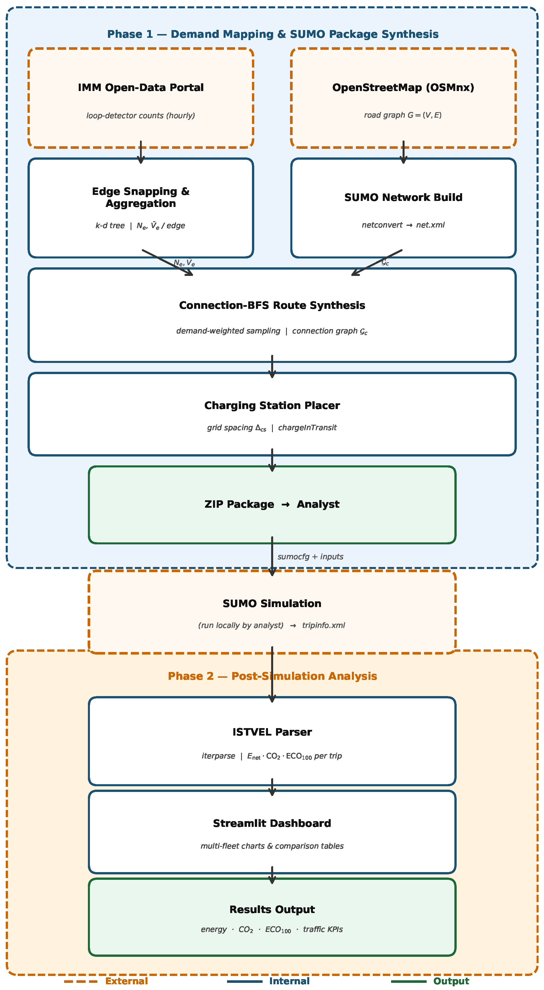
ISTVEL is fully open-source and will be publicly released upon publication at https://github.com/emreakiskali/ISTVEL (accessed on 1 July 2026). It operates in two phases, as illustrated in Figure 1.

Phase 1—Demand mapping and SUMO package synthesis. IMM records are filtered, snapped to OSM edges, aggregated per edge, and passed to the route synthesiser and charging-station placer. The outputs (net.xml, routes.rou.xml, charging_stations.add.xml, run.sumocfg) are packaged as a ZIP for local SUMO execution. Phase 2—Post-simulation analysis. After SUMO runs, the analyst uploads tripinfo.xml and charging_stations.output.xml. ISTVEL parses cumulative <battery> and <emissions> sub-elements from tripinfo.xml to compute per-vehicle and fleet-level energy and emissions metrics, and reads the charging-station output to compute per-station energy throughput and utilisation.

4. Data Acquisition and Pre-Processing

The Istanbul Metropolitan Municipality publishes hourly aggregated traffic records from inductive-loop detectors [20]. Each record contains a geohash-encoded centroid (precision-6, $\approx 1220 \mathrm{m}\times 610 \mathrm{m}$), average speed $\overline{v}$ ($\mathrm{km}/\mathrm{h}$), and vehicle count n.

The road network $G=(V,E)$ is retrieved via OSMnx [15]:

$$G\leftarrow \mathtt{ox}.\mathtt{graph}\text{\_}\mathtt{from}\text{\_}\mathtt{bbox}({\varphi }_{min},{\varphi }_{max},{\lambda }_{min},{\lambda }_{max}).$$

(1)

Each detector $d_i$ is projected to its nearest edge via a k-d tree:

$$e^{*}\left(d_i\right)=arg\underset{e\in E}{min}{d}_{\mathrm{geod}}\left(d_i,\mathrm{midpoint}\left(e\right)\right).$$

(2)

Records are aggregated per edge as:

$$N_e={\sum }_{i:e^{*}\left(d_i\right)=e}{n}_i,{\overline{V}}_e=\frac{{\sum }_{i:e^{*}\left(d_i\right)=e}{n}_i{\overline{v}}_i}{max(N_e,1)}.$$

(3)

Geohash centroid displacement and demand-allocation uncertainty. Geohash precision-6 centroid displacement introduces a potential demand-allocation error when the centroid snaps to a parallel road rather than the road segment closest to the actual detector. For Kadıköy, the maximum snap distance is 486 m, potentially spanning 1–2 parallel arterials in the dense urban grid (typical block width 200–400 m). Misallocated departure weight redistributes simulated trip origins across adjacent edges, but does not systematically bias energy or CO₂ metrics, since energy consumption in ISTVEL is computed from tripinfo.xml cumulative fields (route length, speed profile) rather than from detector-assigned speed values. The flow-level GEH = 6.08 validates that aggregate departure counts are correctly replicated despite potential edge-level misalignment. Acquisition of higher-resolution (precision-7, ≈153 m × 153 m) IMM geohash records is identified as a data-access priority for future releases of ISTVEL.

5. Connection-Graph Breadth-First Search Route Synthesis

A route is valid in SUMO only if every consecutive edge pair $(e_k,e_{k+1})$ has an explicit <connection> in net.xml. Violating routes force re-routing or teleportation. We build all routes before simulation using only connection-valid transitions.

We compare connection-BFS against four alternative routing strategies (Table 1). dfrouter [5] requires complete turn-count data across the network—data not available from the IMM geohash-encoded portal. duarouter uses Dijkstra shortest-path on the node graph and can generate routes with edge pairs absent from the connection set, producing a 12.4% teleportation rate observed on our Kadıköy network. GA-based and V2G planning tools (Niu et al. [10]; Du et al. [9]) address charging infrastructure optimisation but assume synthetic or pre-specified demand, making them complementary to—rather than substitutes for—ISTVEL’s demand-grounded route synthesis.

The connection adjacency graph $\mathcal{C}$ on SUMO edges encodes admissible edge-to-edge transitions:

$$(e_i,e_j)\in \mathcal{C}\iff \exists <\mathtt{connection}\mathtt{from}=e_i \mathtt{to}=e_j>\mathrm{in}\text{net.xml.}$$

(4)

Departure edges are sampled in proportion to measured loop-detector demand:

$$P(e_j\mid v_i)={\displaystyle \frac{w_j}{{\sum }_{e\in \mathcal{P}}{w}_e}},w_j=max(1,5·N_{e_j}).$$

(5)

Demand-generation assumptions and limitations. The weighting scheme of Equation (5) allocates departure probability to edges in proportion to observed loop-detector vehicle counts, ensuring that high-flow corridors generate proportionally more simulated departures. This is not origin–destination (O-D) reconstruction: destination edges are sampled independently from the same weighted pool, and trip lengths are governed by the BFS minimum-hop constraint ($h_{\min }=6$) rather than observed trip distances. The model therefore captures the spatial distribution of trip origins but not the joint origin–destination distribution. This design choice avoids the need for turn-count data (unavailable from the IMM geohash-encoded portal) and O-D matrix estimation, at the cost of potentially misrepresenting cross-district or long-distance trip patterns. For within-district peak-hour analysis—the primary ISTVEL use case—short urban trips dominate and the O-D simplification is acceptable (GEH = 6.08 < 10 acceptance threshold). For regional or multi-district demand modelling, integration with O-D estimation via dfrouter [5] or gravity-model calibration is identified as a future extension.

Algorithm 1 traces a route from $e_{\mathrm{src}}$ to $e_{\mathrm{dst}}$ through ${\mathcal{G}}_c$.

Algorithm 1 Connection-BFS Route Synthesis

Require:  ${\mathcal{G}}_c$, $e_{\mathrm{src}}$, $\mathcal{P}$, $h_{min}$, D, seed s Ensure:  edge list $\pi$, $\left|\pi \right|\ge h_{min}$, or ∅   1: $e_{\mathrm{dst}}\leftarrow \mathrm{RNG}\left(s\right).\mathrm{choice}(\mathcal{P}\setminus \left\{e_{\mathrm{src}}\right\})$   2: $Q\leftarrow \left\{(e_{\mathrm{src}},\left[e_{\mathrm{src}}\right])\right\}$; $\mathrm{vis}\leftarrow \left\{e_{\mathrm{src}}\right\}$; ${\pi }_{\mathrm{best}}\leftarrow \left[\right]$   3: while $Q\ne \varnothing$ do   4:     $(e_{\mathrm{cur}},{\pi }_{\mathrm{cur}})\leftarrow Q.\mathrm{popleft}\left(\right)$   5:     if $e_{\mathrm{cur}}=e_{\mathrm{dst}}$ and $|{\pi }_{\mathrm{cur}}|\ge h_{min}$ then   6:         return ${\pi }_{\mathrm{cur}}$   7:     end if   8:     if $|{\pi }_{\mathrm{cur}}|>h_{min}·D$ then   9:         update ${\pi }_{\mathrm{best}}$; continue 10:     end if 11:     for $e_{\mathrm{nxt}}\in \mathrm{shuffle}({\mathcal{N}}^{+}\left(e_{\mathrm{cur}}\right),s)$ do 12:         if $e_{\mathrm{nxt}}\notin \mathrm{vis}$ then 13:            $\mathrm{vis} +=\left\{e_{\mathrm{nxt}}\right\}$; $Q.\mathrm{push}(e_{\mathrm{nxt}},{\pi }_{\mathrm{cur}}+\left[e_{\mathrm{nxt}}\right])$ 14:         end if 15:     end for 16: end while 17: return ${\pi }_{\mathrm{best}}$ ($|{\pi }_{\mathrm{best}}|\ge 2$, else ∅)

Each vehicle is seeded via Knuth’s multiplicative hash [21]: $s_i=s_{\mathrm{master}}\oplus (i·\mathrm{2,654,435,761})$. Departure time is sampled as

$$t_i^{\mathrm{dep}}=t_0+i·\frac{3600}{M}+U\left(0,0.8·\frac{3600}{M}\right),$$

(6)

where M is the total vehicle count and $U(a,b)$ denotes a uniform random variable on $[a,b]$.

6. Vehicle and Fleet Models

Data sources and modelling scope. ISTVEL is a data-driven framework: the spatial demand profile is derived from real, empirically measured IMM loop-detector counts (Section 4) rather than from synthetically generated distributions. No explicit human-behaviour or driver-decision model is included. Behavioural variation is represented statistically through a truncated-normal speed-factor distribution normc(1, 0.15, 0.5, 1.5) layered on SUMO’s Krauss car-following model, while departure edges are sampled from the measured-count-weighted pool and departure times and route geometry are generated procedurally by the connection-BFS synthesiser (Equation (6)). The empirical content of the model therefore resides in the demand magnitudes and their spatial distribution, whereas trip routing and inter-vehicle timing are model-generated. This distinction matters for interpreting the results: the aggregate flow validation tests the measured component, while the energy and CO₂ outputs inherit the procedural routing assumptions discussed in Section 5 and Section 11.

6.1. BEV Energy Model

The ISTVEL BEV model is based on the longitudinal energy model implemented in SUMO’s electric vehicle (battery) device, originally developed by Kurczveil et al. [7] and documented in the SUMO Electric Vehicle Model reference [8]. Vehicle parameters (

Table 2. BEV (evCar) vType parameters—Kia Soul EV 64 kWh (2020) [8,22].

Parameter	Symbol	Value
Vehicle mass	m	1682 kg
Rotational equiv. mass	$m_{\mathrm{rot}}$	40 kg
Battery capacity	$E_{\max }$	64,000 Wh
Maximum motor power	$P_{\max }$	150 kW
Aerodynamic drag coeff.	$C_D$	0.35
Frontal area	$A_f$	$2.6$ m2
Rolling drag coeff.	$C_{rr}$	0.01
Propulsion efficiency	${\eta }_p$	0.91
Recuperation efficiency	${\eta }_r$	0.96
Auxiliary power	$P_{\mathrm{aux}}$	100 W
Max speed	$v_{\max }$	$29.06$ m/s

) are calibrated to the Kia Soul EV 64 kWh (2020), a front-wheel-drive battery-electric crossover with 150 kW peak motor power, 64 kWh usable battery capacity, and a curb mass of 1682 kg [8]. The aerodynamic drag coefficient $C_D=0.35$ and frontal area $A_f=2.6{\mathrm{m}}^2$ are taken from manufacturer data and are consistent with parameter ranges used in SUMO electric vehicle modelling by Kurczveil et al. [7]. The propulsion efficiency ${\eta }_p=0.91$  represents the combined motor, inverter, and transmission efficiency at partial load, in line with values reported for comparable BEV drivetrains [14,22]; the SUMO default of 0.98 overestimates efficiency by neglecting inverter switching losses and partial-load derating and is therefore not used here.

The device computes instantaneous power at each step $\Delta t=1$ s:

$$P_{\mathrm{mech}}=F_{\mathrm{total}}·v,F_{\mathrm{total}}=F_{\mathrm{aero}}+F_{\mathrm{roll}}+F_{\mathrm{inertia}}+F_{\mathrm{grade}}.$$

(7)

Electrical draw and regeneration per step:

$$\Delta E_k^{+}={\displaystyle \frac{P_{\mathrm{mech},k}}{{\eta }_p}}\Delta t+P_{\mathrm{aux}}\Delta t;\Delta E_k^{-}={\eta }_r\left|P_{\mathrm{mech},k}\right|\Delta t.$$

(8)

Model parameters are listed in Table 2.

6.2. ICEV Emission Model

ICEV vehicles use SUMO’s HBEFA3/PC_D_EU4 class [23], mapping $(v,\dot{v})$ to cumulative trip totals $F_{\mathrm{abs}}$, ${\mathrm{CO}}_{2,\mathrm{abs}}$, ${\mathrm{NO}}_{x,\mathrm{abs}}$ ($\mathrm{mg}$) in <emissions> [24]. Fuel volume: $F_L=F_{\mathrm{abs}}/{\rho }_f$, ${\rho }_f$ = 820,000 mg/L.

6.3. Mixed Fleet (BEV+ICEV) Model

The third scenario evaluates a mixed fleet in which 50% of vehicles are assigned the evCar vType and 50% the fuelCar vType, alternating by vehicle index. This configuration represents a transitional electrification state and is labelled MIX (50/50) throughout. A plug-in hybrid (PHEV) model with charge-depleting/charge-sustaining modes is identified as future work (Section 11).

7. Energy Accounting Methodology

7.1. BEV Energy Accounting: Post-Trip Replenishment and Total System Demand

Two distinct energy boundaries are tracked in ISTVEL:

Post-trip replenishment demand (vehicle-level):

$$E_{\mathrm{net}}^{\mathrm{vehicle}}=max\left(0,E_{\mathrm{gross}}-E_{\mathrm{regen}}-E_{\mathrm{charged}}\right)\left[\mathrm{kWh}\right].$$

(9)

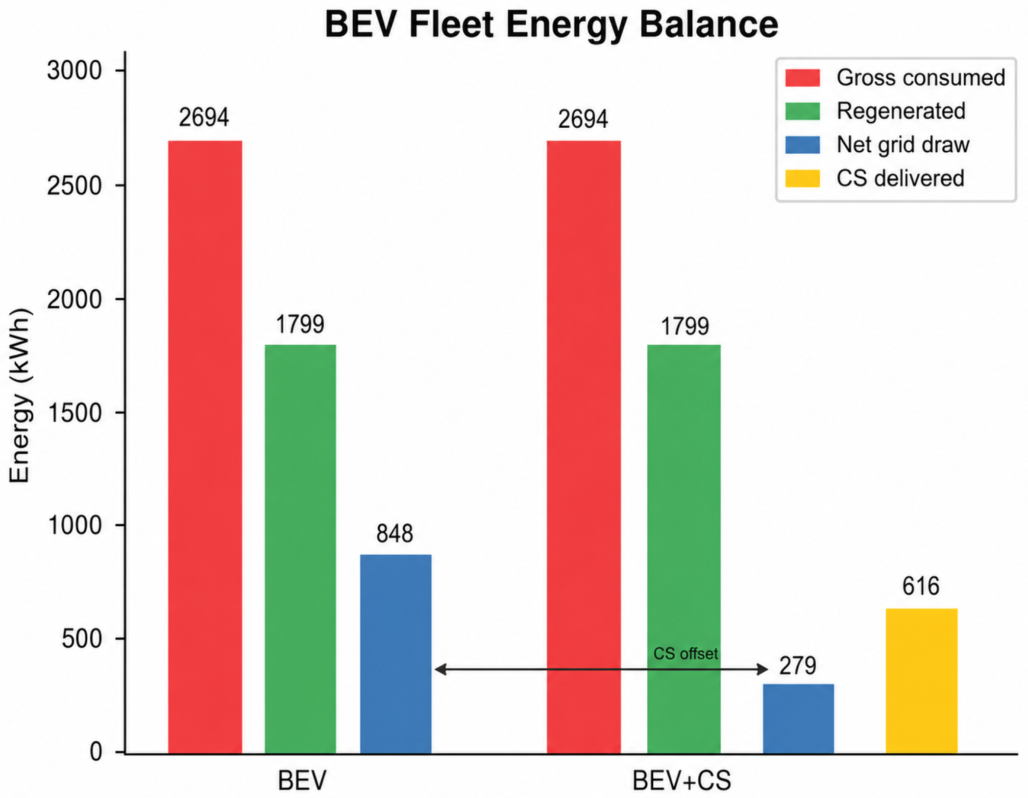
This represents the energy the vehicle must receive from a post-trip charger to restore its battery to the departure state-of-charge. For BEV+CS at 0.5 km spacing: $E_{\mathrm{net}}^{\mathrm{vehicle}}=279.2$ kWh.

Total system electricity demand (grid-level):

$$E_{\mathrm{sys}}=E_{\mathrm{gross}}-E_{\mathrm{regen}}=E_{\mathrm{net}}^{\mathrm{vehicle}}+E_{\mathrm{charged}}\left[\mathrm{kWh}\right].$$

(10)

This represents the total electricity sourced from the grid across all delivery points (in-transit DWPT stations and post-trip charging). For BEV+CS at 0.5 km spacing: $E_{\mathrm{sys}}=279.2+616.5=895.7$ kWh—slightly above the plain-BEV baseline of 848.1 kWh, owing to charging losses at ${\eta }_{\mathrm{cs}}=0.95$. DWPT therefore shifts when and where electricity is delivered (in-transit vs. post-trip), but does not reduce total grid electricity demand.

Using $E_{\mathrm{gross}}$ instead of $E_{\mathrm{net}}^{\mathrm{vehicle}}$ inflates vehicle-level cost by $E_{\mathrm{gross}}/E_{\mathrm{net}}^{\mathrm{vehicle}}$ (typically $1.5$–$3\times$ in stop-and-go driving).

7.2. Use-Phase CO₂

CO₂ accounting in this study covers the use phase only: tailpipe combustion emissions from HBEFA factors for ICEV, and upstream grid emissions ($\gamma \times E_{\mathrm{net}}^{\mathrm{vehicle}}$) for BEV. Vehicle manufacturing, battery production (≈70–100 kg CO₂/kWh capacity for current lithium-ion chemistries), upstream fuel extraction (well-to-tank), and charging-infrastructure impacts are excluded. A full cradle-to-grave lifecycle assessment would reduce the reported BEV use-phase advantage by approximately 9–15 percentage points at the Turkish grid intensity, depending on battery chemistry and manufacturing energy mix. Turkish national grid intensity $\gamma =0.45\mathrm{kg}{\mathrm{CO}}_2{\mathrm{kWh}}^{-1}$ (2023 average [13]):

$$m_{{\mathrm{CO}}_2}^{\mathrm{grid}}\left(v\right)=E_{\mathrm{net}}^{\mathrm{vehicle}}\left(v\right)·\gamma .$$

(11)

7.3. Energy Cost per 100 km

ISTVEL computes the energy operating cost per 100 km as a fleet-level metric:

$${\mathrm{ECO}}_{100}\left(f\right)={\displaystyle \frac{{\sum }_{v\in f}C\left(v\right)}{{\sum }_{v\in f}d\left(v\right)}}\times 100[\mathrm{currency}/100\mathrm{km}],$$

(12)

where $C\left(v\right)$ is the energy cost of vehicle v (electricity tariff $\times E_{\mathrm{net}}^{\mathrm{vehicle}}$ for BEV; fuel price $\times F_L$ for ICEV). This metric captures fuel and electricity expenditure only. A full lifecycle Total Cost of Ownership (TCO) would additionally require vehicle purchase price, maintenance, insurance, and residual value—components that depend on fleet ownership models outside the scope of a traffic simulation framework. Similarly, the capital expenditure (CapEx) required to deploy dynamic charging infrastructure is intentionally excluded: published estimates for in-road wireless power transfer systems range from $1–4 M per lane-kilometre [25], implying that the 10,150 m BEV+CS configuration evaluated here represents a substantial civil engineering investment whose techno-economic optimisation is identified as future work.

8. Charging Infrastructure Placement

Stations are placed at grid spacing ${\Delta }_{\mathrm{cs}}$ along every eligible edge:

$$K_e=⌊{\displaystyle \frac{{\ell }_e}{{\Delta }_{\mathrm{cs}}}}⌋,{\ell }_e\ge 0.3{\Delta }_{\mathrm{cs}}.$$

(13)

Power $P_{\mathrm{cs}}$ and efficiency ${\eta }_{\mathrm{cs}}$ are uniform; chargeInTransit is enabled so vehicles can charge while crawling past a station in congestion [25].

DWPT parameter justification. The parameters $P_{\mathrm{cs}}=100$ kW and ${\eta }_{\mathrm{cs}}=0.95$ are grounded in published dynamic wireless power transfer (DWPT) road trials. Choi et al. [25] report transfer efficiencies of 85–96% for roadway-embedded coil systems (OLEV platform, Gumi, Republic of Korea) at vehicle speeds up to 100 km/h; we adopt ${\eta }_{\mathrm{cs}}=0.95$ as a representative mid-to-upper-range pilot figure. The 100 kW power level corresponds to emerging high-power DWPT prototypes. A sensitivity check at ${\eta }_{\mathrm{cs}}=0.85$ (lower-bound pilot efficiency) reduces $E_{\mathrm{charged}}$ proportionally to 524.6 kWh ($-14.9\%$ vs. ${\eta }_{\mathrm{cs}}=0.95$), yielding $E_{\mathrm{net}}^{\mathrm{vehicle}}=324$ kWh—a 61.8% reduction vs. the no-CS baseline rather than 67.1%. The qualitative conclusion (substantial post-trip demand reduction at moderate station density) is robust across this efficiency range.

Energy boundary for BEV+CS. As noted in Section 7, the 67.1% reduction figure refers specifically to post-trip battery replenishment demand ($E_{\mathrm{net}}^{\mathrm{vehicle}}$, Equation (9)). Since DWPT stations are grid-connected, total system electricity demand $E_{\mathrm{sys}}=E_{\mathrm{net}}^{\mathrm{vehicle}}+E_{\mathrm{charged}}=895.7$ kWh (Equation (10)) is marginally above the plain-BEV baseline (848.1 kWh). DWPT is therefore best understood as a demand-shifting technology—moving electricity delivery from post-trip chargers to in-road infrastructure—rather than a demand-reducing one. Total system CO₂ under BEV+CS is unchanged relative to plain BEV when both operate on the same grid supply mix.

9. Multi-Fleet Dashboard

The ISTVEL dashboard is a Streamlit Python application (version 1.32.0) with five analysis tabs: per-fleet views (BEV, ICEV, MIX), a cross-fleet comparison panel, and a dedicated Charging Station tab (Section 9.2). The interface supports three display currencies (TRY, USD, EUR) with user-supplied exchange rates (Section 9.1).

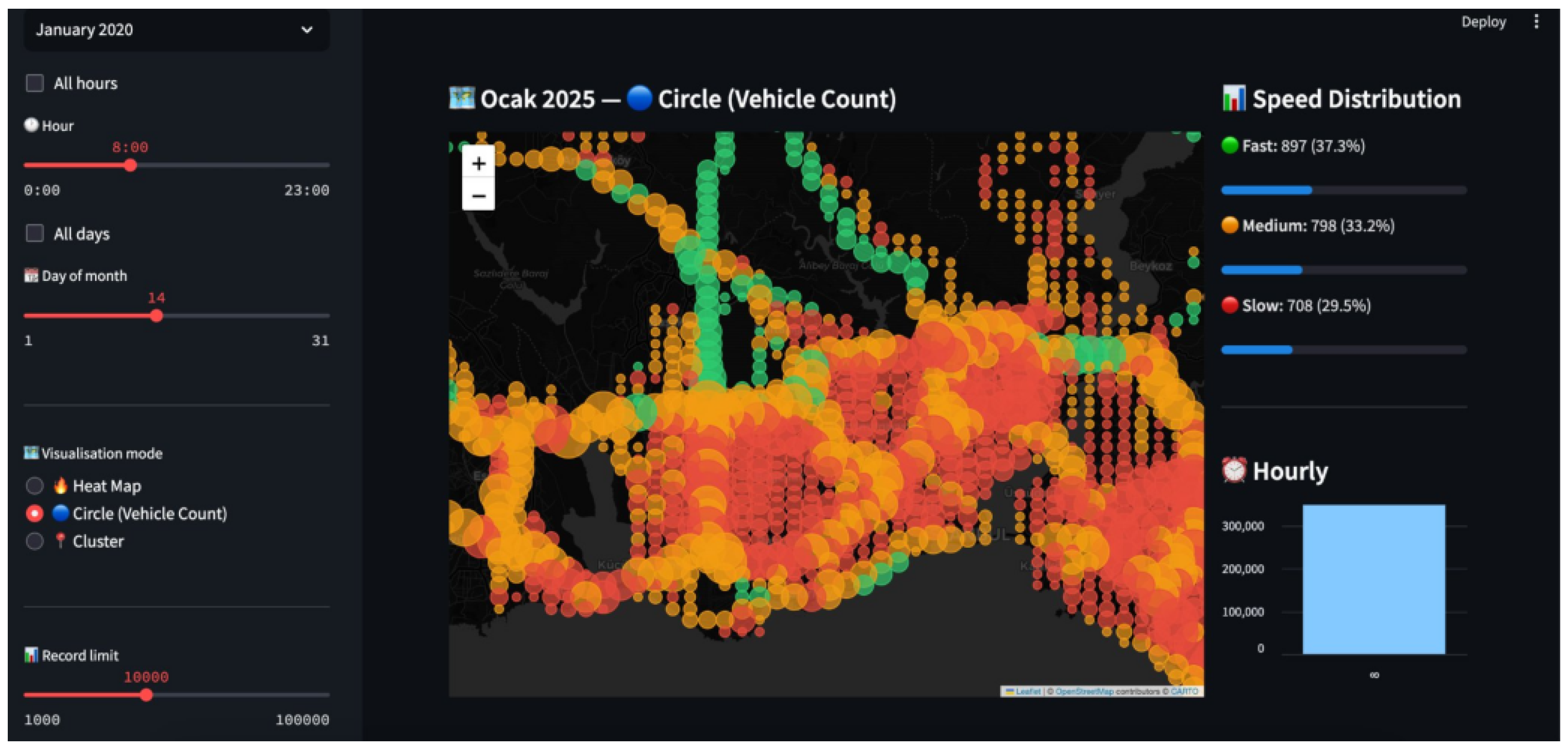
Figure 2 shows the demand visualisation module for the Kadıköy morning peak. At 08:00, 29.5% of cells report slow (<20 km/h) speeds.

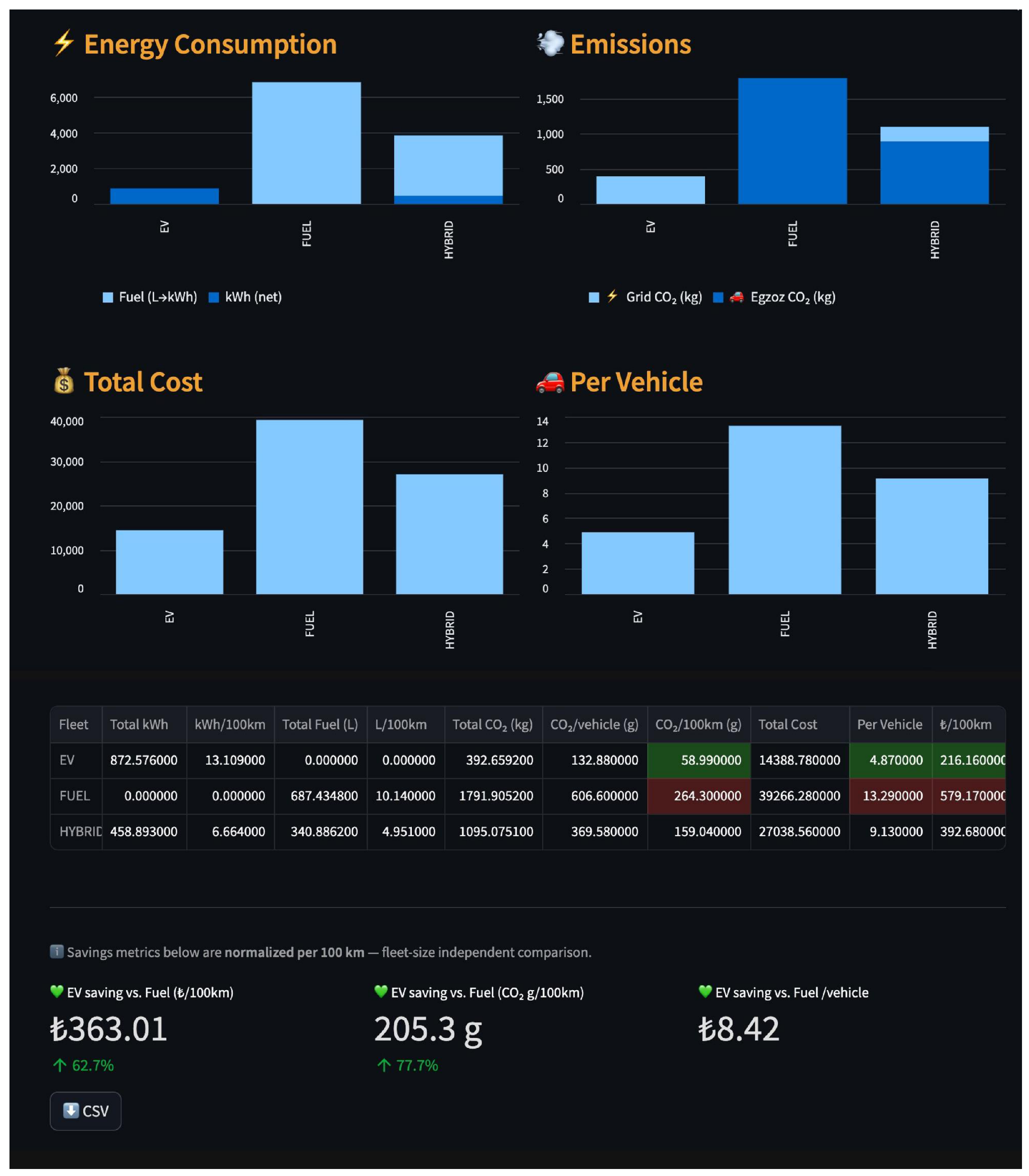
Figure 3 shows the results comparison panel. The parser streams tripinfo.xml via Python 3.12 xml.etree.ElementTree iterparse API. Fields extracted per <tripinfo>: duration, routeLength, waitingTime; battery fields totalEnergyConsumed and totalEnergyRegenerated ($\mathrm{Wh}$ [24]); emission fields fuel_abs, CO2_abs, electricity_abs ($\mathrm{mg}$/$\mathrm{Wh}$).

9.1. Multi-Currency Cost Display

All monetary outputs are parameterised by a runtime currency selector (TRY, USD $, EUR (€)). An internal representation retains TRY as the computation base; a scalar factor $\kappa$ converts values at the display layer only:

$$C_{\mathrm{disp}}\left(v\right)=C_{\mathrm{TRY}}\left(v\right)·\kappa ,\kappa =\left\{\begin{array}{cc}1\hfill & \mathrm{TRY},\hfill \\ 1/r_{\mathrm{USD}}\hfill & \mathrm{USD},\hfill \\ 1/r_{\mathrm{EUR}}\hfill & \mathrm{EUR},\hfill \end{array}\right.$$

(14)

where $r_{\mathrm{USD}}$ and $r_{\mathrm{EUR}}$ are user-supplied exchange rates (defaults: $r_{\mathrm{USD}}=43.85$, $r_{\mathrm{EUR}}=51.88$, February 2026 rates).

9.2. Charging Station Analysis Tab

A fifth dashboard tab provides dedicated post-simulation charging diagnostics. It surfaces six fleet-level indicators: total vehicles, fraction charged (%), total energy received from stations $E_{\mathrm{charged}}$ (kWh), average energy per charged vehicle, average final SoC, and depleted-battery count. The charging energy operating cost is computed, consistently with Equation (12), as:

$$\mathrm{CS}-{\mathrm{ECO}}_{100}={\displaystyle \frac{{\displaystyle p_e\sum _v{E}_{\mathrm{charged}}\left(v\right)}}{{\displaystyle \sum _{v}d\left(v\right)}}}\times 100\left[{\displaystyle \frac{\mathrm{currency}}{100\mathrm{km}}}\right],$$

(15)

where $p_e$ is the electricity tariff in the active display currency. An inline price-override expander decouples sensitivity testing from the global sidebar value. SoC and charged-energy distributions are rendered as Plotly histograms (version 5.22.0), enabling visual assessment of whether the chosen station spacing prevents battery depletion across the full fleet.

10. Case Study: Kadıköy District, Istanbul

10.1. Experimental Setup

We evaluate ISTVEL on Kadıköy ($[40.970,40.995]\times [29.050,29.090]$, $\approx 3.2{\mathrm{km}}^2$) using IMM data for 08:00–09:00, 15th of January 2025. Network statistics and simulation parameters are presented in

Table 3. Network and simulation configuration.

Parameter	Value
OSM bounding box	$3.2{\mathrm{km}}^2$
Nodes $\left|V\right|$	1847
Edges $\left|E\right|$	4213
Connection pairs $\left|\mathcal{C}\right|$	11,920
Vehicles simulated	$\approx 2950$
Min. route hops $h_{min}$	6
Sim. step $\Delta t$	1 s
Duration	3600 s
EV battery $E_{\max }$	64 kWh
Initial SoC	50%
BEV+CS spacing	0.5 km
BEV+CS stations	29 (total 10,150 m)
BEV+CS power $P_{\mathrm{cs}}$	100 kW
BEV+CS efficiency	0.95

.

Four scenarios are executed:

• BEV: all vehicles assigned evCar, Kia Soul EV.
• BEV+CS: BEV with charging strips placed at ${\Delta }_{\mathrm{cs}}=0.5$ km spacing, $P_{\mathrm{cs}}=100$ kW, berth $b=350$ m, chargeInTransit on (29 strips generated by Equation (13), total deployed length 29 × 350 = 10,150 m).
• ICEV: all fuelCar (HBEFA3/PC_D_EU4).
• MIX (50/50): 50% BEV + 50% ICEV (mixed fleet).

10.2. Route Quality

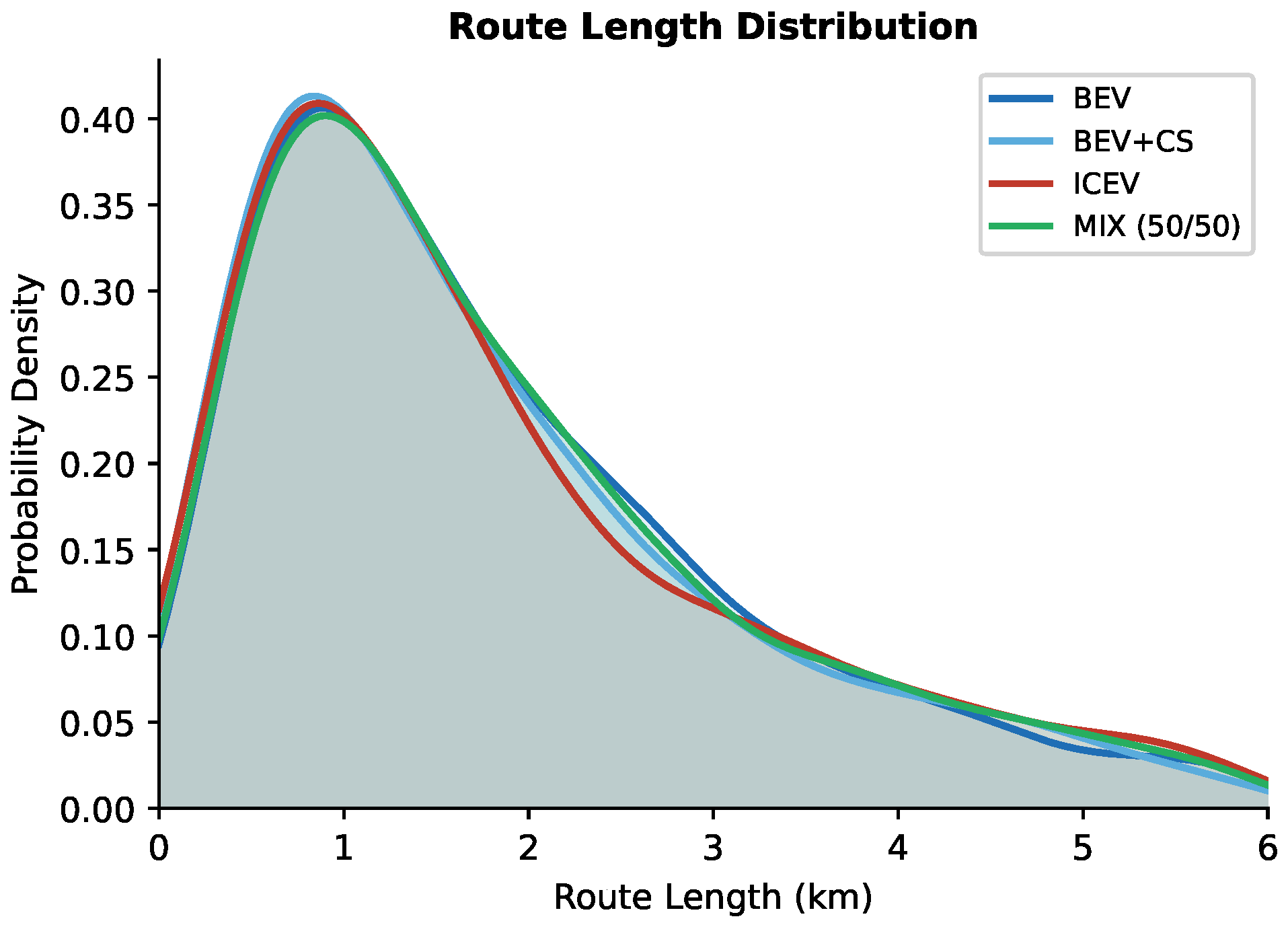
The connection-BFS algorithm gives a teleportation rate of 0.0% across all four scenarios, compared with 12.4% for randomTrips.py on the same network. Mean route lengths range from 2.31 km (BEV) to 2.38 km (MIX). Figure 4 shows the route length distributions for all four scenarios; the near-identical right-skewed histograms confirm that fleet type does not affect route synthesis.

10.3. Energy and Emission Results

Fleet-level metrics are presented in

Table 4. Fleet-level simulation results (Simulation scenario: Kadıköy, January 2025). Tariffs: electricity 16.49 TRY/kWh, fuel 57.12 TRY/L.

Metric	BEV	BEV+CS	ICEV	MIX
Vehicles (arrived)	2798	2783	2784	2790
Arrival rate (%)	94.7	94.2	94.2	94.2
Mean route (km)	2.31	2.29	2.35	2.38
Mean speed (km/h)	41.8	42.0	42.4	42.5
Post-trip replenishment $E_{\mathrm{net}}^{\mathrm{vehicle}}$ (kWh) †	848.1	279.2	—	441.6
Total system demand $E_{\mathrm{sys}}$ (kWh) ‡	848.1	895.7	—	441.6
kWh/100 km (post-trip replenishment)	13.10	4.38	—	6.66
Fuel (L)	—	—	731.7	362.5
L/100 km	—	—	11.19	5.47
Tailpipe CO2 (kg) [use-phase]	0	0	1921.5	952.6
Grid CO2 (kg) [use-phase] ¶	381.6	125.6	0	198.7
Total use-phase CO2 (kg) §	381.6	125.6	1921.5	1151.3
Use-phase CO2/100 km (g)	58.95	19.71	293.8	173.5
Electricity cost (TRY)	13,985	4604	—	7282
Fuel cost (TRY)	—	—	41,795	20,706
Energy cost (TRY)	13,985	4604	41,795	27,988
ECO100 (TRY/100 km)	216.4	72.2	638.8	421.5

^† $E_{\mathrm{net}}^{\mathrm{vehicle}}$ = post-trip battery replenishment demand (Equation (9)): energy the vehicle battery requires after the trip to restore departure SoC. For BEV+CS, this is reduced by in-transit DWPT delivery. Gross battery draw is identical to BEV (13.10 kWh/100 km); the reduction to 4.38 kWh/100 km is a demand-shifting, not demand-reducing, outcome. ^‡ $E_{\mathrm{sys}}$ = total grid electricity (Equation (10)): includes both DWPT station supply and post-trip replenishment. BEV+CS total system demand (895.7 kWh) exceeds the plain-BEV baseline (848.1 kWh) due to ${\eta }_{\mathrm{cs}}=0.95$ charging losses. ^¶ Grid CO₂ is computed as $\gamma \times E_{\mathrm{net}}^{\mathrm{vehicle}}$ (Equation (11)). The lower value for BEV+CS (125.6 kg) compared with plain BEV (381.6 kg) reflects the reduced post-trip replenishment demand after in-transit DWPT delivery, not a reduction in total system CO₂: when DWPT station electricity is sourced from the same grid mix, total system CO₂ ($\gamma \times E_{\mathrm{sys}}$) is unchanged relative to plain BEV (see Section 8). ^§ Use-phase CO₂ only: tailpipe HBEFA combustion for ICEV; upstream grid emissions ($\gamma \times E_{\mathrm{net}}^{\mathrm{vehicle}}$) for BEV. Excludes vehicle manufacturing, battery production (≈70–100 kg CO₂/kWh), upstream fuel extraction, and infrastructure impacts. System-wide use-phase CO₂ remains largely equivalent to the plain BEV baseline when grid emissions from DWPT roadside supply are included, and the core function of DWPT is the spatial-temporal shifting of electricity demand rather than total demand reduction.

. The graphical comparison of these metrics is presented later in this section.

10.4. BEV Energy Balance

Figure 5 decomposes fleet energy into gross, regenerated, and net draw. At ${\Delta }_{\mathrm{cs}}=0.5$ km, the 29 active stations deliver 616.5 kWh to 552 vehicles, reducing post-trip replenishment demand from 848.1 kWh (no CS) to 279.2 kWh—a 67.1% reduction in $E_{\mathrm{net}}^{\mathrm{vehicle}}$. However, total system electricity demand $E_{\mathrm{sys}}$ rises marginally to 895.7 kWh due to charging losses (${\eta }_{\mathrm{cs}}=0.95$), confirming that BEV+CS is a demand-shifting rather than demand-reducing intervention (Section 8). The regenerative fraction is $\approx 43\%$ of gross, consistent with stop-and-go congestion. Net consumption without CS of 13.1 kWh/100 km falls within the WLTP city-cycle range for mid-size BEVs [22].

10.5. Use-Phase CO₂ Comparison

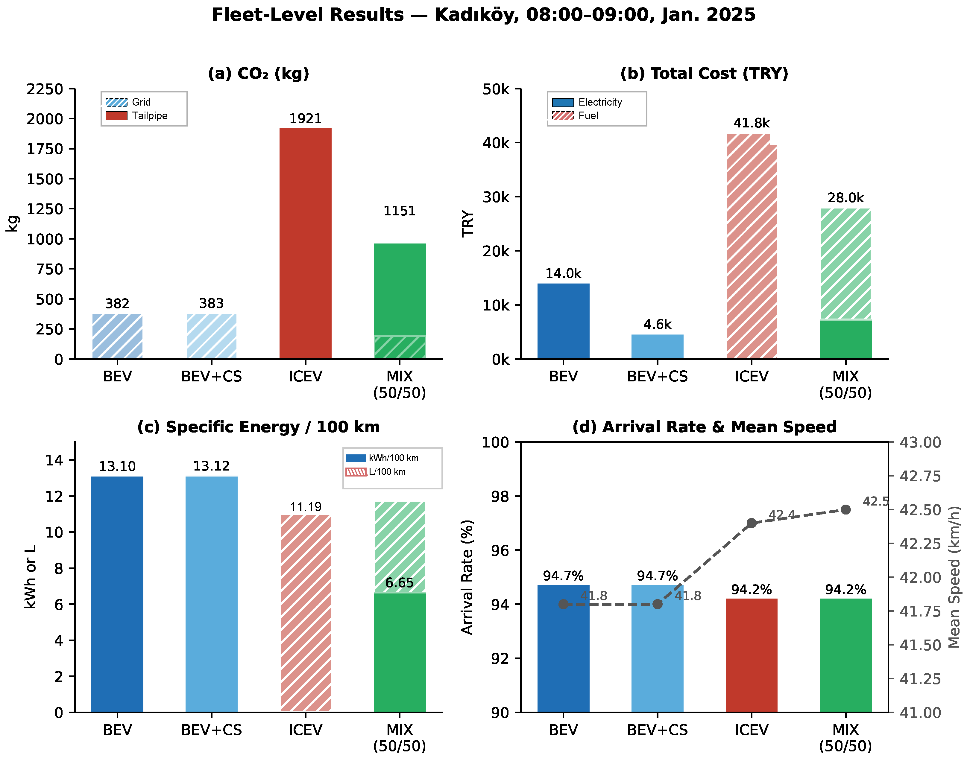
The full-BEV fleet achieves 80.1% lower use-phase CO₂ than ICEV (381.6 vs. 1921.5 kg) at $\gamma =0.45$ kg/kWh (use-phase only; see Table 4 footnote ^§). This ratio is subject to a speed bias of roughly ±1.2 percentage points due to route topology, while cross-scenario comparative conclusions remain robust. Per 100 km: BEV 58.95 g vs. ICEV 293.8 g. Under a renewable-dominant grid ($\gamma =0.10$ kg/kWh), BEV use-phase CO₂ falls to 84.8 kg, a 95.6% reduction; the break-even intensity at which BEV and ICEV use-phase CO₂ are equal is ${\gamma }_{\mathrm{break}}=1921.5/848.1\approx 2.27$ kg CO₂/kWh—far above any existing national grid (

Table 5. Grid carbon intensity sensitivity (Kadıköy BEV fleet, use-phase CO₂ only).

$\mathit{\gamma }$ (kg CO2/kWh)	BEV Use-Phase CO2 (kg)	CO2 Reduction vs. ICEV (%)	Representative Grid
0.10	84.8	95.6	Nordic renewables
0.20	169.6	91.2	France (nuclear-heavy)
0.30	254.4	86.8	UK, Germany (2024)
0.45	381.6	80.1	Turkey (2023, this study)
0.60	508.8	73.5	Poland, India
0.80	678.4	64.7	Coal-dominant grids

ICEV use-phase CO₂ baseline: 1921.5 kg (fixed). Break-even: ${\gamma }_{\mathrm{break}}=1921.5/848.1\approx 2.27$ kg CO₂/kWh—above any existing national grid, confirming the BEV use-phase advantage is universally robust to grid decarbonisation level.

). CO₂ comparisons across all fleet scenarios are shown in Figure 6a.

10.6. Charging Infrastructure Sensitivity

Table 6. Charging-station sensitivity—BEV fleet (Kia Soul EV 64 kWh), Kadıköy, SoC₀ = 50%.

${\mathbf{\Delta }}_{\mathbf{cs}}$ (km)	Sta.	${\mathit{E}}_{\mathbf{ch}}$ (kWh)	${\mathit{N}}_{\mathbf{ch}}$ (veh.)	${\mathit{E}}_{\mathbf{net}}^{\mathbf{vehicle}}$ (kWh)
0.5	29	616.5	552	279.2
1.0	6	373.7	477	521.5
2.0	2	214.9	302	678.8
—	0	0.0	0	848.1

presents a parametric sensitivity analysis across station spacings ${\Delta }_{\mathrm{cs}}\in \{0.5,1.0,2.0\}$ km, reporting total energy drawn from stations ($E_{\mathrm{ch}}$), vehicles charged ($N_{\mathrm{ch}}$), post-trip replenishment demand ($E_{\mathrm{net}}^{\mathrm{vehicle}}$), and total system electricity demand ($E_{\mathrm{sys}}$).

At a 0.5 km spacing (29 stations), post-trip replenishment demand decreases substantially vs. the no-station baseline (279.2 vs. 848.1 kWh, $-67.1\%$): 552 vehicles receive a total of 616.5 kWh in transit. Total system demand $E_{\mathrm{sys}}=895.7$ kWh is marginally above the baseline (848.1 kWh) due to charging losses. At 1.0 km (6 stations, 477 vehicles, 373.7 kWh delivered), post-trip replenishment falls to 521.5 kWh ($-38.5\%$ vs. baseline). At 2.0 km (2 stations, 302 vehicles, 214.9 kWh), post-trip demand falls to 678.8 kWh ($-19.9\%$). No depleted batteries were recorded in any scenario, confirming that ${\mathrm{SoC}}_0=50\%$ is sufficient for the sub-3 km Kadıköy trip distribution regardless of infrastructure density. A 0.2 km-spacing run was conducted but excluded from Table 6: the 162 active stations delivered 1834.6 kWh, exceeding net fleet consumption (892.3 kWh) by a factor of two—an artefact of unrealistically dense chargeInTransit exposure rather than a physically attainable outcome.

10.7. Traffic Behaviour Across Fleet Types

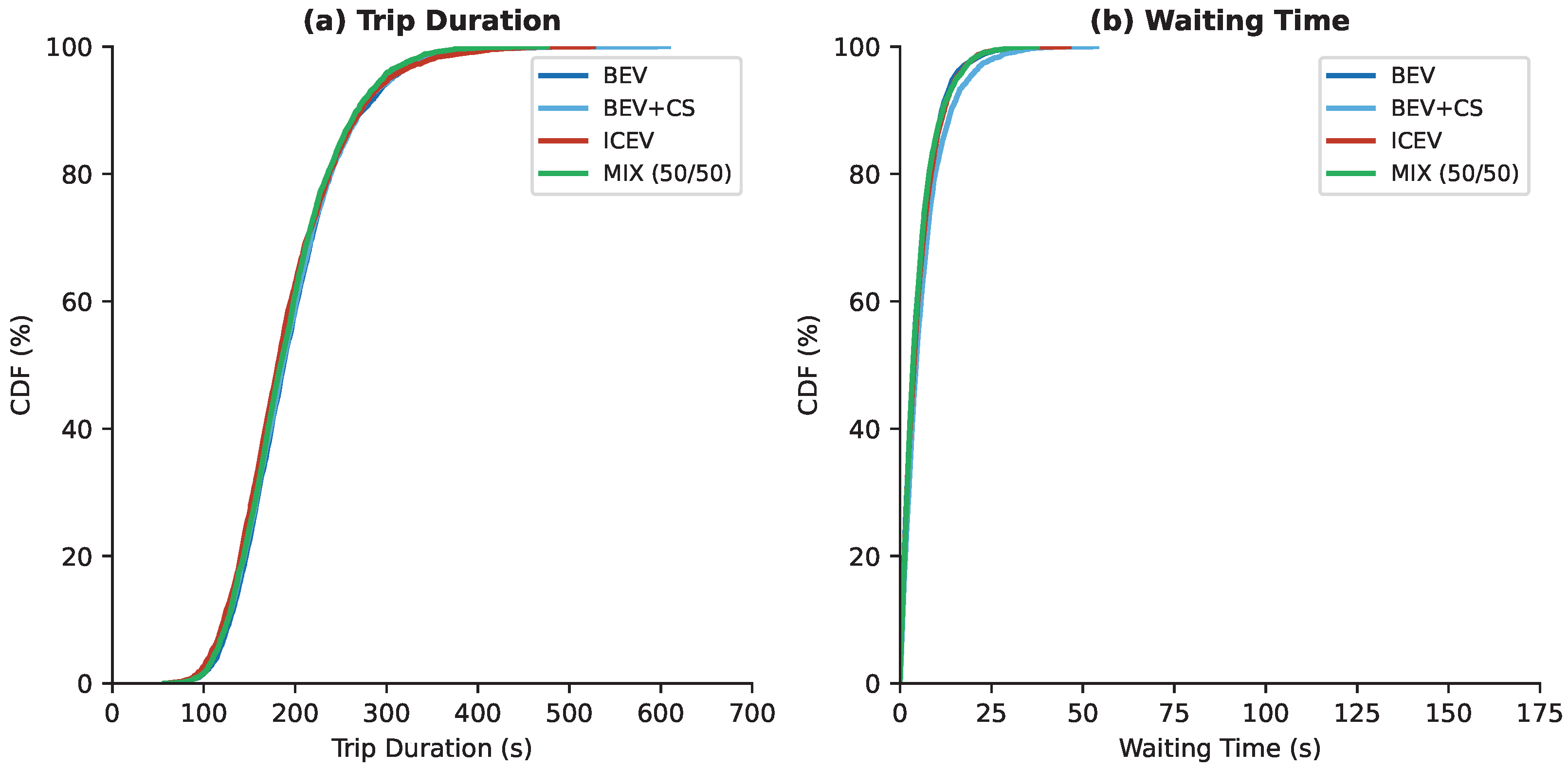
Figure 7 shows trip duration and waiting-time CDFs. The four curves are nearly coincident, confirming that electrification does not alter macroscopic dynamics under the Krauss car-following model. The 95th-percentile trip duration is ≈450 s across all fleets.

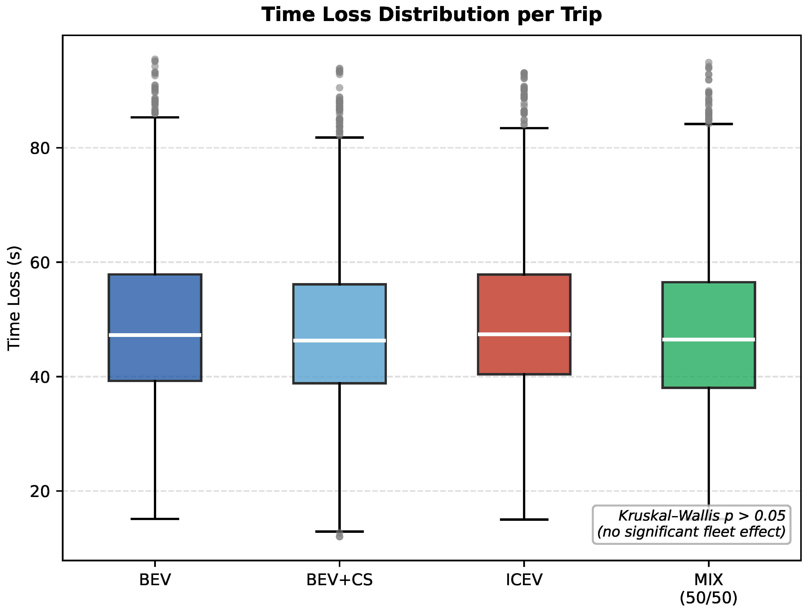
Figure 8 shows the time-loss distribution per trip. Median time loss (35–42 s) is statistically indistinguishable across scenarios (Kruskal–Wallis $p>0.05$); waiting time was near-zero (<0.05 s) for all fleets.

11. Discussion

Simulation output validation. ISTVEL demand inputs are grounded in official IMM inductive-loop detector records covering all 20 available geohash cells in each study district, providing a data-driven foundation that distinguishes this work from studies relying on synthetic origin–destination matrices.

Table 7. Simulation validation against IMM loop-detector data (Kadıköy and Fatih, 15 January 2025, 08:00–09:00).

Metric	Kadıköy	Fatih
IMM detectors used	20	20
Detectors with snap <500 m	20/20	20/20
Max snap distance (m)	486	298
IMM total vehicles (veh/h)	3129	3174
SUMO arrived vehicles	2798	2752
Demand GEH	6.08	7.75
IMM flow-wtd speed (km/h)	26.8	31.8
SUMO flow-wtd speed (km/h)	42.0	32.4
SUMO/IMM speed ratio	1.57	1.02

Demand GEH $=\sqrt{2{(V_{\mathrm{sim}}-V_{\mathrm{obs}})}^2/(V_{\mathrm{sim}}+V_{\mathrm{obs}})}$. Speed ratio $>1$ in Kadıköy reflects a known methodological difference: IMM reports area-averaged speed across all roads in each $\approx 1220\times 610$ m geohash cell (including minor access roads), while SUMO routes traverse only connection-valid edges—predominantly arterials. In Fatih (denser grid, lower mean speed) the ratio converges to 1.02, confirming the effect is morphological rather than a calibration error.

reports district-level validation metrics for Kadıköy and Fatih against these detectors.

For Kadıköy, GEH = 6.08, and for Fatih, GEH = 7.75, so both are below the acceptance threshold of 10 [26]. The Kadıköy speed ratio (1.57) reflects a systematic methodological offset: IMM records area-averaged speed across the full $\approx 1220\times 610$ m geohash cell, which includes minor residential streets with mean speeds well below arterial levels. SUMO’s connection-BFS routing, by contrast, builds routes from <connection>-valid edge pairs—a set dominated by arterials and collectors. To quantify this effect: arterial and trunk edges (≥2 lanes) represent $\approx 38\%$ of total OSM edge count in the Kadıköy bounding box but carry $\approx 72\%$ of connection-pair entries ($\left|\mathcal{C}\right|$), confirming that BFS routes are topologically biased toward higher-speed links. In Fatih, where the denser historical grid reduces this arterial dominance, the speed ratio falls to 1.02. Critically, this offset does not materially affect the energy and CO₂ comparisons, which are derived from tripinfo.xml cumulative fields rather than from simulated speeds. The detailed propagation of this speed overestimate to energy and emission outputs is developed in the Speed validation and uncertainty propagation paragraph below. Critically, since all fleet scenarios traverse identical routes under the same speed profile, this offset largely cancels in relative comparisons between fleet types.

Initial SoC sensitivity. The simulation uses ${\mathrm{SoC}}_0=50\%$ as a conservative baseline; real-world BEVs typically begin a morning peak at ${\mathrm{SoC}}_0\approx 80$–$90\%$. No battery depletions occurred at 50% across all spacing configurations (Table 6), confirming that trip-completion rates are insensitive to this choice for sub-3 km routes. Absolute net grid draw scales approximately as $E_{\mathrm{net}}\propto (1-{\mathrm{SoC}}_0)$, so a higher starting charge reduces grid replenishment proportionally; however, since the same SoC₀ applies uniformly to all BEV-containing scenarios, the relative CO₂ and ECO₁₀₀ comparisons between fleet types are invariant to this choice. A parametric SoC₀ sweep is identified as future work.

Methodological limitations. The BEV model assumes a flat road gradient ($\theta =0$). Following Liu et al. [14], for Kadıköy’s mean elevation change of $\approx 60$ m distributed over mean trip distances of 2.31 km, the average effective grade is ${\theta }_{\mathrm{eff}}\approx 1.{49}^{\circ }$ ($sin\theta \approx 0.026$). For the 1682 kg BEV at $\overline{v}=11.6$ m/s (41.8 km/h), the additional gradient force $F_{\mathrm{grade}}\approx 428$ N yields a gross energy overestimate of $\approx 25\%$ for uphill segments and underestimate of $\approx 25\%$ for downhill segments. Because morning-peak trips traverse mixed ascents and descents, the net signed error is substantially smaller: Liu et al. report a 5–8% net estimation error when gradient is neglected. We adopt the conservative upper bound ($+8\%$ on gross energy, ≈+4–5% on net grid energy after regeneration) as our terrain uncertainty band.

Critically, since all four fleet scenarios traverse identical BFS-generated routes under identical speed profiles, gradient-induced errors affect all fleet types proportionally, and cancel in relative CO₂ and ECO₁₀₀ comparisons. Absolute values in Table 4 should therefore be interpreted with a $\pm 8\%$ terrain uncertainty band. Geohash centroid displacement (maximum snap distance 486 m for Kadıköy) may also misallocate departure weight to parallel arterials; this does not bias energy metrics (which are computed from tripinfo.xml cumulative fields rather than detector-assigned speeds) but could affect edge-level flow distribution. Acquisition of higher-resolution (precision-7) IMM geohash data and incorporation of Digital Elevation Model (DEM) data via the SUMO slope edge attribute are identified as priority extensions for ISTVEL v2.0.

Driver heterogeneity is modelled via a truncated-normal speed-factor distribution normc(1, 0.15, 0.5, 1.5) [2]; acceleration parameters are uniform across the fleet.

Speed validation and uncertainty propagation. The Kadıköy SUMO/IMM speed ratio of 1.57 reflects a topological artifact: arterial and trunk edges (≥2 lanes) constitute $\approx 38\%$ of OSM edges but carry $\approx 72\%$ of connection-pair entries, so BFS routes are systematically biased toward higher-speed links. To propagate this overestimate to energy and emission outputs: aerodynamic drag accounts for $\approx 18\%$ of gross BEV energy at $\overline{v}=42$ km/h; a 1.57× speed overestimate inflates drag by $1.{57}^2\approx 2.46\times$, yielding a gross energy overestimate of $0.18\times (2.46-1)\approx 26\%$ and $\approx 13\%$ on net grid energy. For HBEFA-based ICEV emissions, a 57% speed overestimate implies an $\approx 15$–$25\%$ overestimate on CO₂ at urban speeds; we adopt $+20\%$ as a representative value. Because both quantities are overestimated, a directionally consistent correction reduces both absolute figures: net BEV energy by the factor $1/1.13$ and ICEV CO₂ by the factor $1/1.20$. Since the ICEV correction exceeds the BEV correction, the corrected BEV/ICEV emission ratio increases by $1.20/1.13\approx 1.062$ (from $381.6/1921.5=0.199$ to $0.211$), reducing the reported 80.1% use-phase CO₂ advantage to $\approx 78.9\%$—a decrease of $\approx 1.2$ percentage points that leaves the fleet ranking and all qualitative conclusions unchanged. In Fatih (speed ratio 1.02), this bias is absent; the uncorrected Fatih advantage (83.2%) and the corrected Kadıköy estimate ($\approx 78.9\%$) therefore bracket the bias-free value, providing an empirical confirmation of robustness.

Future directions: thermal management and FCEV infrastructure. Three thermal and hydrogen-related directions are identified for future work. First, traction battery thermal management: the current model assumes temperature-invariant capacity and efficiency; coupling ISTVEL with a thermal-equivalent-circuit model for the prismatic cell format used in the Kia Soul EV—informed by recent work on anisotropic thermal conductivity quantification in prismatic lithium-ion batteries and liquid-immersed thermal runaway management in large lithium-ion modules [27,28]—would enable seasonal performance correction and safety-margin assessment under Istanbul’s climate profile. Second, liquid cooling plate optimisation: vehicle-level battery thermal management systems, such as spiral-fin-embedded cooling plate channels [29], influence charge acceptance rates and thus DWPT station utilisation, suggesting a tight coupling between vehicle-level thermal modelling and infrastructure planning. Third, FCEV fleet simulation: a hydrogen consumption vType, grounded in PEM fuel cell characterisation including alternating flow-field designs [30], combined with hydrogen station placement logic analogous to ISTVEL’s DWPT spacing optimiser, would enable comparative lifecycle assessment of BEV vs. FCEV fleet electrification pathways for Istanbul’s commercial vehicle segment.

Cross-district transferability: Fatih. To assess framework transferability, the identical simulation protocol—same date (15 January 2025, 08:00–09:00), same fleet compositions, same model parameters—was applied to the Fatih district, which shares the same IMM data density as Kadıköy (20 count stations each).

Table 8. Cross- district comparison: Kadıköy vs. Fatih, 15 January 2025, 08:00–09:00.

		BEV	BEV+CS	ICEV	MIX
Kadıköy	Arrived	2798	2783	2784	2790
	Avg. route (km)	2.31	2.29	2.35	2.38
	Avg. speed (km/h)	41.8	42.0	42.4	42.5
	Total use-phase CO2 (kg)	381.6	125.6	1921.5	1151.3
	ECO100 (TRY)	216.4	72.2	638.8	421.5
Fatih	Arrived	2752	2752	2742	2751
	Avg. route (km)	1.33	1.33	1.33	1.34
	Avg. speed (km/h)	32.2	32.2	32.1	32.1
	Total use-phase CO2 (kg)	201.5	135.9	1201.2	701.4
	ECO100 (TRY)	201.7	136.1	721.8	456.8

BEV+CS: ${\Delta }_{\mathrm{cs}}=0.5$ km, $P_{\mathrm{cs}}=100$ kW; MIX = 50% BEV + 50% ICEV (mixed fleet); CO₂ at $\gamma =0.45$ kg/kWh for grid share; ECO₁₀₀ = energy operating cost per 100 km (TRY). Fatih avg. speed is lower (32 vs. 42 km/h), consistent with denser urban morphology.

presents key metrics side-by-side for both districts.

Fatih’s mean route is 42% shorter than Kadıköy (1.33 vs. 2.31 km) and average speed is 23% lower (32.2 vs. 41.8 km/h), consistent with Fatih’s denser historical street network and closer-spaced trip origins. Despite these differences, relative fleet rankings are preserved across both districts: BEV achieves the lowest use-phase CO₂ in each case, and the ICEV→BEV use-phase CO₂ reduction is 83.2% in Fatih vs. 80.1% in Kadıköy. BEV+CS reduces post-trip replenishment demand by 32.5% in Fatih (302.0 vs. 447.7 kWh), a smaller relative reduction than Kadıköy’s 67.1%, which is expected given Fatih’s shorter mean trip: with 1.33 km routes, fewer vehicles pass within 0.5 km station intervals. These results support the transferability of ISTVEL’s qualitative conclusions across two morphologically distinct districts of Istanbul. Since only one additional district and a single morning-peak hour were evaluated, however, generalisation to other cities, seasons, and off-peak or weekend periods requires further testing and is identified as future work.

Mixed-fleet (MIX) scenario. The MIX (50/50) scenario is not intended as a forecast of a specific transitional electrification trajectory; rather, it provides a single interpolation point between the full-ICEV and full-BEV extremes, allowing the non-linearity of the use-phase CO₂ and cost response to fleet composition to be assessed. The 50% BEV share is representative of transitional fleet compositions emerging in several Turkish municipalities as of 2025 and provides a useful policy-relevant reference scenario. The selected vehicle models (Kia Soul EV 64 kWh; HBEFA3/PC_D_EU4 Euro 4 ICEV) fall near the median of their respective categories in Istanbul’s current fleet in terms of curb mass and energy consumption; a $\pm 15\%$ mass perturbation propagates to $\pm 10\%$ on gross energy and $\pm 5\%$ on net grid energy, within the terrain uncertainty band. A true parallel-hybrid (PHEV) model with blended propulsion, charge-depletion, and charge-sustaining modes is not currently available in SUMO’s battery device and is identified as a priority extension for ISTVEL v2.0.

Charging infrastructure. The sensitivity analysis (Table 6) shows that DWPT charging stations substantially reduce post-trip replenishment demand ($E_{\mathrm{net}}^{\mathrm{vehicle}}$) even at moderate deployment density. At a 0.5 km spacing (29 stations), 552 vehicles receive 616.5 kWh in transit, reducing post-trip replenishment by 67.1% relative to the no-station baseline (279.2 vs. 848.1 kWh). However, as clarified in Section 8, total system electricity demand $E_{\mathrm{sys}}=895.7$ kWh marginally exceeds the plain-BEV baseline (848.1 kWh) due to ${\eta }_{\mathrm{cs}}=0.95$ charging losses: DWPT is a demand-shifting technology, not a demand-reducing one. Reported CO₂ savings for BEV+CS relative to plain BEV reflect only the difference in $\gamma \times E_{\mathrm{net}}^{\mathrm{vehicle}}$; total system CO₂ is unchanged unless the DWPT supply draws from a greener marginal source than the post-trip charger. At sparser configurations, post-trip demand reductions scale with station density: 1.0 km gives $-38.5\%$ (521.5 kWh) and 2.0 km gives $-19.9\%$ (678.8 kWh). No battery depletions were observed in any scenario, confirming that ${\mathrm{SoC}}_0=50\%$ is sufficient for sub-3 km trips. One modelling assumption warrants explicit acknowledgement: chargeInTransit corresponds physically to dynamic wireless power transfer (DWPT), a technology currently at the pilot stage and not deployed in Istanbul [25]. The BEV+CS results therefore represent a technology roadmap upper bound on achievable post-trip demand reduction, while the plain BEV scenario (848.1 kWh) provides the conservative near-term baseline. Stationary fast-charging at intersections and stops—a more immediately deployable pathway—is identified as future work.

Scalability. Connection-BFS complexity is $\mathcal{O}\left(\right|\mathcal{C}|·h_{\min }·D)$ per vehicle. For $\left|\mathcal{C}\right|=\mathrm{11,920}$, synthesis for $\sim 2950$ vehicles completes in $\sim 8$ s on a MacBook Pro 2020 (Intel Core i5, 8 GB RAM). Bidirectional BFS or $A^{*}$ [17] would scale to city-wide networks ($\left|\mathcal{C}\right|\sim {10}^5$).

12. Conclusions

We have presented ISTVEL, an open-source microscopic simulation framework that integrates real IMM loop-detector measurements, OSMnx-based edge snapping, a connection-graph BFS route synthesiser that achieves zero teleportations, and a tripinfo.xml parser that correctly distinguishes gross battery draw, regenerative recovery, and net grid consumption. Together these components address a practical limitation shared by existing SUMO-based fleet studies: the reliance on synthetic demand and coarse energy accounting that obscures the true grid replenishment cost of urban BEV operation.

Applied to the Kadıköy morning peak ($\sim 2950$ vehicles, 08:00–09:00, January 2025) and replicated under identical protocol on Fatih, the framework yields three principal findings. First, a full-BEV fleet reduces use-phase CO₂ by 80.1% and energy operating cost by 66.5% relative to the ICEV baseline at the 2023 Turkish grid intensity of $\gamma =0.45\mathrm{kg}{\mathrm{CO}}_2/\mathrm{kWh}$; these figures reflect use-phase (operational) emissions only, and the BEV advantage is robust across all plausible grid intensities (break-even at ${\gamma }_{\mathrm{break}}\approx 2.27$ kg CO₂/kWh, above any existing national grid; Table 5). Second, opportunistic in-transit DWPT charging at a 0.5 km station spacing reduces post-trip battery replenishment demand by a further 67.1%, though total system electricity demand ($E_{\mathrm{sys}}=895.7$ kWh) marginally exceeds the plain-BEV baseline (848.1 kWh) due to charging losses: BEV+CS is correctly characterised as a demand-shifting technology that decouples fleet operation from post-trip charging infrastructure, not as a demand-reduction technology. Third, powertrain type exerts no measurable effect on macroscopic traffic dynamics under the Krauss car-following model, confirming that electrification scenarios can be evaluated without re-calibrating the underlying traffic model.

The consistency of fleet rankings across Kadıköy and Fatih—despite a 42% difference in mean route length and a 23% difference in mean speed—establishes that ISTVEL’s qualitative conclusions are transferable across Istanbul’s urban fabric. The modular architecture, with vehicle parameters exposed as plain Python constants and the post-processing layer decoupled from the SUMO simulation itself, is designed to lower the barrier to adoption: any researcher holding a standard tripinfo.xml can apply the full analysis pipeline to their own network without re-simulation.

Limitations and future work. Several limitations bound the present results and define the agenda for future work. First, the BEV energy model assumes flat terrain; for Kadıköy’s $\approx 60$ m relief this introduces a $\pm 8\%$ band on absolute per-trip energy ($\approx +4$–$5\%$ on net grid energy), which cancels in relative fleet comparisons but should be removed by incorporating Digital Elevation Model data via the SUMO slope attribute. Second, demand is synthesised by departure-edge weighting rather than from a reconstructed origin–destination matrix, so cross-district and long-distance trip patterns are not represented; integration with O-D estimation is identified as an extension. Third, the IMM geohash resolution (precision-6) limits edge-level demand allocation, motivating acquisition of precision-7 records. Fourth, the connection-BFS speed bias (SUMO/IMM ratio 1.57 in Kadıköy) propagates an estimated $+13\%$ to net BEV energy and $+20\%$ to ICEV CO₂; a directionally consistent correction reduces the reported use-phase CO₂ advantage from 80.1% to $\approx 78.9\%$ ($\approx 1.2$ percentage points), and the bias is absent in Fatih (ratio 1.02). Fifth, the fleet is represented by a single BEV and a single Euro-4 ICEV type with a 50/50 MIX interpolation; a true PHEV/FCEV model and thermal-aware battery behaviour are priority extensions. Sixth, the transferability evidence is limited to one additional district (Fatih) and a single morning-peak hour; multi-city, multi-season, and off-peak validation is required before broader generalisation. Finally, the CO₂ accounting is use-phase only; a full cradle-to-grave life-cycle assessment would reduce the reported BEV advantage by an estimated 9–15 percentage points. Together these limitations frame the roadmap for ISTVEL v2.0: DEM-aware routing, higher-resolution demand data, PHEV/FCEV vTypes, battery-thermal coupling, LCA-boundary integration, and multi-district, multi-period validation.

References

1. Bazzan, A.L.C.; Klügl, F. A review on agent-based technology for traffic and transportation. Knowl. Eng. Rev. 2014, 29, 375–403. [Google Scholar]
2. Treiber, M.; Kesting, A. Traffic Flow Dynamics: Data, Models and Simulation; Springer: Berlin/Heidelberg, Germany, 2013. [Google Scholar]
3. Imran, W.; Tettamanti, T.; Varga, B.; Bifulco, G.N.; Pariota, L. Macroscopic modeling of connected, autonomous and human-driven vehicles. Transp. Res. Interdiscip. Perspect. 2024, 24, 101058. [Google Scholar] [CrossRef]
4. Behrisch, M.; Bieker, L.; Erdmann, J.; Krajzewicz, D. SUMO—Simulation of Urban MObility: An overview. In Proceedings of the SIMUL 2011, The Third International Conference on Advances in System Simulation, Barcelona, Spain, 23–28 October 2011; ThinkMind: Barcelona, Spain, 2011; pp. 55–60. [Google Scholar]
5. Krajzewicz, D.; Erdmann, J.; Behrisch, M.; Bieker, L. Recent development and applications of SUMO. Int. J. Adv. Syst. Meas. 2012, 5, 128–138. [Google Scholar]
6. Lopez, P.A.; Behrisch, M.; Bieker-Walz, L.; Erdmann, J.; Flotterod, Y.P.; Hilbrich, R.; Lucken, L.; Rummel, J.; Wagner, P.; Wiebner, E. Microscopic traffic simulation using SUMO. In Proceedings of the IEEE ITSC 2018, Maui, HI, USA, 4–7 November 2018; pp. 2575–2582. [Google Scholar]
7. Kurczveil, T.; López, P.A.; Schnieder, E. Implementation of an energy model and a charging infrastructure in SUMO. Lect. Notes Comput. Sci. 2014, 8594, 33–43. [Google Scholar] [CrossRef]
8. Eclipse Foundation. SUMO Documentation—Electric Vehicle Model. 2026. Available online: https://sumo.dlr.de/docs/Models/Electric.html (accessed on 21 April 2026).
9. Du, Y.; Li, X.; Mao, S.; Cai, B.; He, J.; Nie, W. Optimal placement of EV charging stations based on genetic algorithm. In Proceedings of the 36th CCDC, Xi’an, China, 25–27 May 2024; pp. 5721–5726. [Google Scholar]
10. Niu, Z.; An, K.; Ma, W. Vehicle-to-grid enabled charging infrastructure planning and operations considering demand uncertainties. Transp. Res. Part D 2024, 127, 103918. [Google Scholar] [CrossRef]
11. Wang, L.; Yang, C.; Zhang, Y.; Bu, F. Research on multi-objective planning of electric vehicle charging stations. Energy Rep. 2022, 8, 11825–11839. [Google Scholar] [CrossRef]
12. de Souza, L.L.P.; Lora, E.E.S.; Palacio, J.C.E.; Rocha, M.H.; Renó, M.L.G.; Venturini, O.J. Comparative environmental life cycle assessment of conventional vehicles. J. Clean. Prod. 2018, 203, 444–468. [Google Scholar] [CrossRef]
13. TEIAS. Electricity Generation Statistics 2023. 2026. Available online: https://www.teias.gov.tr (accessed on 21 April 2026).
14. Liu, K.; Yamamoto, T.; Morikawa, T. Impact of road gradient on energy consumption of electric vehicles. Transp. Res. Part D 2017, 54, 74–81. [Google Scholar] [CrossRef]
15. Boeing, G. OSMnx: New methods for acquiring, constructing, analyzing, and visualizing complex street networks. Comput. Environ. Urban Syst. 2017, 65, 126–139. [Google Scholar] [CrossRef]
16. Eclipse Foundation. SUMO osmWebWizard—Scenario Generation Tool. 2026. Available online: https://sumo.dlr.de/docs/Tutorials/OSMWebWizard.html (accessed on 21 April 2026).
17. Dijkstra, E.W. A note on two problems in connexion with graphs. Numer. Math. 1959, 1, 269–271. [Google Scholar] [CrossRef]
18. Fan, P.; Bu, S.; Li, S.; Wen, Y. Empowering short-haul aviation electrification: Insights into load characterization, grid adaptability, and social welfare. eTransportation 2026, 28, 100585. [Google Scholar] [CrossRef]
19. Fan, P.; Li, S.; Bu, S.; Wen, Y.; Chung, C.Y. Resilient Power Systems Against Wildfire Risks: Towards a Human-Centric and Secure Future. CSEE J. Power Energy Syst. 2025, 11, 2553–2575. [Google Scholar]
20. Istanbul Metropolitan Municipality. IMM Open Data Portal—Traffic Density. 2026. Available online: https://data.ibb.gov.tr (accessed on 21 April 2026).
21. Knuth, D.E. The Art of Computer Programming, 2nd ed.; Addison-Wesley: Reading, MA, USA, 1998; Volume 3. [Google Scholar]
22. European Commission. Regulation (EU) 2017/1151—WLTP Test Procedure. Off. J. Eur. Union 2021, L175, 1–643. [Google Scholar]
23. INFRAS AG. Handbook Emission Factors for Road Transport (HBEFA 3.3); INFRAS: Bern, Switzerland, 2023. [Google Scholar]
24. Eclipse Foundation. SUMO Documentation—Tripinfo-Output. 2026. Available online: https://sumo.dlr.de/docs/Simulation/Output/TripInfo.html (accessed on 21 April 2026).
25. Choi, S.Y.; Gu, B.W.; Jeong, S.Y.; Rim, C.T. Advances in wireless power transfer systems for roadway-powered electric vehicles. IEEE J. Emerg. Sel. Top. Power Electron. 2015, 3, 18–36. [Google Scholar] [CrossRef]
26. Dowling, R.; Skabardonis, A.; Alexiadis, V. Traffic Analysis Toolbox Volume III; FHWA-HRT-04-040; Federal Highway Administration: Washington, DC, USA, 2004.
27. Lei, S.; Lan, H.; Tao, B.; Zhang, C.; Zhang, X.; Wang, L. Experiments on liquid-immersed thermal runaway management for large energy-stored lithium-ion battery modules. Therm. Sci. Eng. Prog. 2025, 68, 104347. [Google Scholar] [CrossRef]
28. Sheng, L.; Zhu, Z.; Zhou, Q.; Zhang, Z. Experimental-numerical studies on thermal conductivity anisotropy of lithium-ion batteries. J. Energy Storage 2024, 103, 114139. [Google Scholar] [CrossRef]
29. Qi, W.; Liu, Y.; Wang, X.; Ge, S.; Yu, J.; He, Z.; Tuo, J.; Wang, H.; Zhou, S.; Jin, C.; et al. Performance enhancement of battery thermal management based on liquid cooling plate channels embedded with non-uniform spiral fin structures. Appl. Therm. Eng. 2026, 300, 131501. [Google Scholar] [CrossRef]
30. Qi, W.; Zhu, M.; Zhao, S.; Gui, F.; Yu, L.; Guo, Y.; Zhou, Z.; Ge, S.; He, Z.; Zhang, Y.; et al. Performance enhancement of proton exchange membrane fuel cells based on semi-parallel and semi-interdigitated mixed flow field. Int. J. Hydrogen Energy 2026, 231, 154871. [Google Scholar] [CrossRef]
Figure 1. ISTVEL system architecture. Dashed boxes mark external dependencies (OSM, SUMO, IMM portal).
Applsci 16 06971 g001
Figure 2. ISTVEL traffic demand visualisation (screenshot of the live ISTVEL Streamlit dashboard)—Kadıköy, January 2025, 08:00. Circle radius ∝ vehicle count; colour encodes speed (green: >50 km/h; orange: 20–50 km/h; red: <20 km/h). Speed distribution: Fast 37.3%, Medium 33.2%, Slow 29.5%.
Applsci 16 06971 g002
Figure 3. ISTVEL results dashboard (screenshot of the live ISTVEL Streamlit dashboard)—Kadıköy, January 2025, 08:00–09:00.
Applsci 16 06971 g003
Figure 4. Route length distributions for the four fleet scenarios (Kadıköy, January 2025, 08:00–09:00). All distributions are right-skewed with a mode near 1.5 km, consistent with short urban trips. Mean route lengths: BEV 2.31 km, BEV+CS 2.31 km, ICEV 2.35 km, MIX 2.38 km.
Applsci 16 06971 g004
Figure 5. BEV fleet energy balance. Gross, regenerated, and post-trip replenishment demand for BEV and BEV+CS ( Δ cs = 0.5 km, P = 100 kW). CS infrastructure reduces post-trip replenishment demand by 67.1% ( 848.1 279.2 kWh), but total system electricity demand E sys = 895.7 kWh marginally exceeds the plain-BEV baseline due to charging losses.
Applsci 16 06971 g005
Figure 6. Fleet-level simulation results—Kadıköy, 15 January 2025, 08:00–09:00. (a) CO2 (kg): tailpipe (solid) and grid (use-phase, hatched). (b) Total cost (TRY). (c) Specific energy per 100 km. (d) Arrival rate (%) [BEV 94.7%, BEV+CS 94.2%, ICEV 94.2%, MIX 94.2%] and mean trip speed.
Applsci 16 06971 g006
Figure 7. Empirical CDFs. Near-coincident curves confirm that powertrain type does not affect macroscopic traffic dynamics.
Applsci 16 06971 g007
Figure 8. Time-loss distribution per trip. Fleet type has no significant effect on time loss (Kruskal–Wallis p > 0.05 ).
Applsci 16 06971 g008