Competing-Risks Time-to-Event Modeling Using the Generalized Gamma Distribution Under Progressive Type-II Censoring

Abstract

Modeling time-to-event data without accounting for risk factors may lead to biased conclusions. Therefore, researchers sometimes assume the existence of competing risks to accurately model life data. Furthermore, since medical research can be time-consuming and costly, experimenters may consider optimizing their use of resources by employing a censoring plan, such as a progressive Type-II censoring scheme. This study investigates statistical inference for a competing-risks model based on Stacy’s generalized gamma distribution under the latter censoring scheme. A couple of frequentist estimation methods—namely, maximum likelihood estimation and maximum product-of-spacings estimation—are used to obtain point estimates of the model parameters. Using the point estimators, asymptotic confidence intervals are constructed alongside two bootstrapping confidence intervals—namely, the percentile and Studentized bootstrap confidence intervals. Monte Carlo simulations are used to numerically examine the performance of both point and interval estimation using appropriate criteria. Overall, the simulations indicate that maximum product-of-spacings estimation outperforms maximum likelihood estimation, particularly in estimating the shape parameter under heavier censoring. The practical illustration of Stacy’s competing-risks model is achieved by analyzing two real medical datasets concerning pneumonia in intensive care and leukemia stem cell transplantation. Overall, the information criteria confirm that Stacy’s competing-risks model provides a robust fit relative to its submodels, offering a highly flexible framework for complex survival data.

1. Introduction

The risk of developing disease is a universal aspect of human life, whether from communicable or non-communicable sources. Risk factors such as obesity and diabetes can increase susceptibility to certain illnesses, exposing individuals to multiple potential outcomes. In medical studies, competing risks arise when the occurrence of one type of event precludes the observation of others. For example, in cancer-specific mortality research, death from causes other than cancer (such as stroke or heart attack) is considered a competing risk. Properly accounting for competing risks is essential for accurate statistical inference, as neglecting them can yield biased results and misleading conclusions. For further details, see the monograph reported in [1] and other recent reviews [2,3].

Suppose that the time of death is declared for a patient of old age with some serious medical issues. Thus, various risk factors, in addition to age, contribute to mortality. Hence, incorporating the concept of competing risks helps model lifetimes more precisely, which improves future clinical-trial planning, treatment design, and medical decision-making. From a statistical viewpoint, the times of death declarations are time-to-event data common in survival analysis. When at least two factors can cause death, investigators are dealing with time-to-event data analysis in the context of competing risks. This type of data consists of successive failure times, each with an indicator of the failure cause.

In statistical literature, Cox’s competing-risks model is often used to analyze competing-risks data [4]. Although it was introduced over six decades ago, it received notable attention from several researchers. Numerous recent works have focused on developing competing-risks models using various censoring schemes and lifetime distributions. For example, Ref. [5] explored comparative life testing using jointly censored samples in the exponential competing-risks framework. Ref. [6] considered progressively Type-II-censored competing-risks data in which the underlying lifetimes follow a linear–exponential distribution. Ref. [7] introduced estimation procedures for competing-risks models with adaptive progressively Type-II-censored Rayleigh lifetime data. Ref. [8] investigated statistical inference for competing-risks samples under a joint Type-II censoring scheme, focusing on the Weibull distribution. Ramadan [9] examined statistical inference in competing-risks models for Akshaya sub-distributions under Type-II censoring. Other noteworthy contributions include [10], which studied a competing-risks model based on the generalized inverted exponential distribution for independent failure modes under progressive Type-II censoring. Ref. [11] discussed inference for a competing-risks model utilizing the Weibull distribution with an improved adaptive progressive Type-II censoring plan. Ref. [12] developed inference methods for competing-risks models with latent failure times drawn from the Kumaraswamy-G family of distributions within a unified progressive hybrid censoring scheme. Furthermore, Ref. [13] proposed an expectation-maximization algorithm for parameter estimation in the Birnbaum-Saunders distribution with censored competing-risks data, and Ref. [14] employed a similar EM algorithm for the inverse Weibull distribution. Ref. [15] introduced a novel additive generalized linear–exponential competing-risks model. More recently, Ref. [16] considered inference for independent competing risks, following the inverse Lomax distribution using a Type-II generalized hybrid censored sample. Ref. [17] assessed reliability functions in competing-risks models using adaptive progressively Type-II-censored data and real datasets (such as datasets concerning small electrical appliances and X-ray–exposed male mice) with the XGamma distribution as the parent model. Recently, Ref. [18] considered Stacy’s competing=-risks model based on Stacy’s generalized gamma distribution [19], which offers greater robustness and flexibility than existing models. Theoretically, this model extends competing-risks models based on the exponential, Weibull, and gamma distributions. Methodologically, this flexibility enables nested model comparison and provides a unified framework for assessing whether simpler models are sufficient.

In a recent study by Alam et al. [18], the main assumption was that the random sample was complete, with no missing data. In the statistical literature, there are many causes of missing data, including censoring, which was considered by some of the research contributions mentioned above. Across diverse fields of research, including medical research and survival analysis, researchers may encounter situations with censored data, where the time-to-event data under study are partially unknown, since individuals participating in a study might drop out or the study may end before the event of interest occurs. This is common due to time constraints and financial or ethical considerations. These challenges are particularly significant in long-duration research. There are various types of data censoring, including conventional, progressive, and hybrid censoring. Sometimes, the censoring scheme is classified as Type-I or Type-II. For more details about censoring schemes, see [20,21,22].

Various censoring schemes under competing risks have been considered for common lifetime distributions, such as the exponential and Weibull distributions, among others. Ref. [23] proposed a competing-risks model under progressive Type-II censoring, assuming independent exponential failure distributions and using both classical and Bayesian methods for statistical inference. Ref. [24] investigated a competing-risks model for incomplete censored data, where failure causes are independently distributed according to generalized exponential distributions. Ref. [25] assumed failure times with independent exponential distributions, considering a Type-II progressively hybrid censoring scheme for competing risks, which effectively exhibited the utilization of experimental resources and time with efficient statistical results. Ref. [26] analyzed a competing-risks model under progressive Type-II censoring with independent failure times, following a Weibull distribution with a common shape parameter but different scale parameters, and discussed optimal progressive censoring plans and different optimality criteria. Ref. [27] developed classical and Bayesian inferential procedures for competing risks under a generalized progressive hybrid censoring scheme, considering exponential lifetimes. Ref. [28] studied maximum likelihood and Bayesian estimators of a competing-risks model under an adaptive progressive Type-II censoring scheme, assuming exponential lifetimes. Ref. [29] studied a competing-risks model under adaptive progressively Type-II censoring, considering a Weibull distribution with different scale and shape parameters for both independent and dependent competing risks. Ref. [30] performed a statistical inference study on a competing-risks model under an improved adaptive Type-II progressive censoring scheme. The study assumed that the lifetimes of competing failure causes are independent and exponentially distributed with distinct parameters. Ref. [11] investigated a competing-risks model under an improved adaptive Type-II progressive censoring scheme, where failure times were independently Weibull-distributed with a common shape parameter and various scale parameters. Under progressively Type-II censoring schemes, competing-risks models have been studied assuming different lifetime distributions. A study by [6] considered progressively Type-II-censored competing-risks data in which the underlying lifetimes follow a linear–exponential distribution. Ref. [9] examined statistical inference in competing-risks models for Akshaya sub-distributions under Type-II censoring. Ref. [31] proposed a competing-risks model based on the inverted Topp–Leone distribution, while Ref. [32] investigated an inverted exponential Rayleigh competing-risks model. Other noteworthy contributions include that of Farghal et al. [10], who studied a competing-risks model based on the generalized inverted exponential distribution for independent failure modes under progressive Type-II censoring. Ref. [33] derived likelihood estimated and both asymptotic and bootstrap confidence intervals for a competing-risks model when failure times follow a Dagum distribution. Monte Carlo studies and real datasets illustrated the applicability of the Dagum model for heavy-tailed, skewed lifetimes. Ref. [34] assumed that the independent latent causes of failure follow a generalized linear–exponential distribution, used maximum likelihood and maximum product-of-spacings estimation approaches to estimate the model parameters, and constructed approximate and bootstrap confidence intervals. The robustness of these methods was illustrated through simulation studies and real-data analyses.

Existing competing-risks models are often structurally restricted to monotonic or bathtub hazard families, rendering them insufficient for the modeling of complex failure patterns frequently observed in medical data. Furthermore, while recent applications of Stacy’s Generalized Gamma (GG) model [18] have introduced the flexibility necessary to capture diverse hazard shapes, they have been strictly limited to complete datasets. Unlike standard lifetime distributions such as the Weibull and Gompertz distributions, which are structurally confined to monotonic or bathtub hazard shapes, the GG distribution intrinsically accommodates increasing, decreasing, bathtub, and unimodal hazard rates without prior structural assumptions. Furthermore, while modern survival approaches such as frailty models are designed to account for unobserved heterogeneity or cluster-level dependencies, the proposed framework specifically operates within a latent minimum of independent lifetimes. The aim of this study is to bridge this gap by extending the contribution of Alam et al. [18] to consider Stacy’s GG competing-risks model under a progressive Type-II censoring (PT-IIC) scheme. This specific combination advances the state of the art by providing a methodologically and computationally rigorous framework that models complex hazard behaviors while directly accounting for the systematic dropout and experimental constraints inherent in long-term medical and biomedical research. It captures realistic experimental scenarios in which objects under study are systematically excluded to minimize experimental cost and time, offering a unified analytical framework for diverse application areas. For instance, suppose a clinical trial for leukemia treatment uses progressive censoring. This allows researchers to efficiently analyze patient outcomes while accounting for competing risks, such as death from cancer relapse versus chemotherapy complications. Since trials often last for years, it is impractical to follow every survivor to the end of the study. The stepwise approach systematically excludes specific survivors from the control group at different stages, such as after a certain number of relapses. This approach benefits the medical field by reducing long-term costs; providing a statistical framework that accounts for patients who withdraw from the study for various reasons; and, most importantly, enabling more accurate estimation of the cumulative relapse rate. This ensures that disease risk is not overestimated by ignoring other causes of death, enabling faster, more accurate assessments of the treatment plan. A statistical model is characterized by the parameters to be estimated; therefore, to evaluate this robust framework and ensure more efficient estimation under heavy censoring, maximum likelihood estimators (MLEs) and maximum product-of-spacing estimators (MPSEs) are obtained, and their performance is studied through Monte Carlo simulation.

The remainder of this paper is organized as follows. Section 2 provides a description of the model used in this study and the censoring scheme. Section 3 and Section 4 discuss the estimation methods of points and the confidence intervals of model parameters. A Monte Carlo simulation study is conducted in Section 5 to evaluate the performance of the proposed estimation procedures. Two medical datasets are analyzed in Section 6. To validate its parametric robustness, the flexibility of the proposed GG model is explicitly benchmarked against modern semi-parametric spline-based hazard approaches in the preceding section. The paper is concluded in Section 7.

2. Model Description

Suppose that the underlying problem is modeled by Cox’s competing-risks model; thus, the following assumptions must be made:

1.

The individual (i.e., patient orparticipant) fails only due to any of the k independent causes of failure.

2.

The lifetimes of the objects (or subjects) under study ($X_1,\dots ,X_n$) are independent and identically distributed random variables (i.e., a random sample). Also, suppose that for $i=1,\dots ,n$, each lifetime can be redefined as $X_i=\min \left\{X_{i1},X_{i2},\dots ,X_{ik}\right\}$ such that $X_{i1},X_{i2},\dots ,X_{ik}$ are latent failure times corresponding to the j different independent competing risk factors.

Without loss of generality, suppose that there are two independent competing risks (i.e., $k=2$); moreover, assume that the underlying model has a similar shape parameter, that is, the model considered in this study is a four-parameter Stacy GG model rather than the six-parameter model considered by Alam et al. [18]. While an increase in the number of parameters may lead to a higher maximized log likelihood, it often induces numerical instability and parameter redundancy. Over-parameterized distributions often exhibit flat likelihood surfaces, which complicate the convergence of estimation methods and increase estimator variance. Therefore, a superior fit must be evaluated not merely by proximity to the observed data but also by the model’s ability to remain identifiable and stable, as measured by penalized information criteria such as the Akaike Information Criterion (AIC) and the Bayesian Information Criterion (BIC). See [35] in this connection and [36] for advances in model selection. Let $X_{ij}$ denote the time-to-event datum caused by risk j such that $i=1,\dots ,n$. If $X_{ij}$ follow the Stacy GG distribution [19] with a scale parameter of ${\lambda }_j>0$ and shape parameters of $\alpha >0$ and $\beta >0$, where $j=1,2,\dots ,k$, then the probability density function (PDF) and survival function (SF) are given by

$$f_j\left(x,\alpha ,\beta ,{\lambda }_j\right)={\displaystyle \frac{\beta }{{\lambda }_j\Gamma \left(\frac{\alpha }{\beta }\right)}}{\left({\displaystyle \frac{x}{{\lambda }_j}}\right)}^{\alpha -1}{e}^{-{\left({\displaystyle \frac{x}{{\lambda }_j}}\right)}^{\beta }},x>0$$

(1)

and

$$S_j(x;\alpha ,\beta ,{\lambda }_j)={\displaystyle \frac{\Gamma \left(\frac{\alpha }{\beta },{\left[\frac{x}{{\lambda }_j}\right]}^{\beta }\right)}{\Gamma \left(\frac{\alpha }{\beta }\right)}},x>0$$

(2)

respectively, where $\Gamma \left({\displaystyle \frac{\alpha }{\beta }}\right)$ is the gamma function, while $\Gamma \left({\displaystyle \frac{\alpha }{\beta }},{\left[{\displaystyle \frac{x}{{\lambda }_j}}\right]}^{\beta }\right)$ is the upper incomplete gamma function defined mathematically as follows:

$$\Gamma \left({\displaystyle \frac{\alpha }{\beta }}\right)={\int }_0^{\infty }{x}^{{\displaystyle \frac{\alpha }{\beta }}-1}{e}^{-x}dx$$

and

$$\Gamma \left({\displaystyle \frac{\alpha }{\beta }},{\left[{\displaystyle \frac{x}{{\lambda }_j}}\right]}^{\beta }\right)={\int }_{{\left({\displaystyle \frac{x}{{\lambda }_j}}\right)}^{\beta }}^{\infty }{x}^{{\displaystyle \frac{\alpha }{\beta }}-1}{e}^{-x}dx.$$

Suppose that n individuals are subjected to the experiment. This researchers aims to acquire a random sample of lifetimes—say, $X_1,X_2,\dots ,X_n$—such that $X_i=\min \left\{X_{i1},X_{i2}\right\}$, where $X_{ij}$ represents the latent failure (i.e., death) time of the i-th item due to the j-th cause of failure. However, due to time and cost constrains, the authorsdecided to employ a PT-IIC scheme, which is described as follows. Suppose a progressive censoring scheme ($R_1,R_2,\dots ,R_m$) is predefined and m is the targeted sample ($m\le n$). At the time of first failure, $R_1$ surviving individuals are removed randomly from from the set of remaining individuals ($n-1$). Subsequently, $R_2$ individuals are withdrawn randomly from the set of remaining individuals ($n-2-R_1$) at the time of second failure. This process proceeds until the mth event occurs. The progressive censoring scheme satisfies ${\sum }_{k=1}^n{R}_k=n-m$. The conventional Type-II right censoring scheme is obtained whenever $R_1=R_2=\cdots =R_{m-1}=0$ and $R_m=n-m$, while if $R_1=R_2=\cdots =R_m=0$, then a complete sample is acquired. For this study, the failure mechanism based on the PT-IIC scheme is characterized as follows:

1.

The total number of observed failures is $m\le n$, while the the total number of censored units is $n-m$.

2.

If the failure of unit i is associated with cause j, the cause of failure is specified through an indicator function ($I({\delta }_i=j)$).

3.

The number of observed failures due to the first risk is $m_1={\sum }_{i=1}^{m}I({\delta }_i=1)$, while $m_2={\sum }_{i=1}^{m}I({\delta }_i=2)$ is the number of observed failures due to the second risk.

The resulting PT-IIC sample is expressed as follows:

$$(X_{1:m:n},{\delta }_1,R_1),(X_{2:m:n},{\delta }_2,R_2),\dots ,(X_{m:m:n},{\delta }_m,R_m),\mathrm{where}{X}_{1:m:n}<\cdots <X_{m:m:n}.$$

(3)

3. Estimation Methods

While the statistical literature offers a diverse array of parameter estimation techniques, this study focuses on two prominent frequentist approaches: the maximum likelihood estimation (MLE) method and the maximum product-of-spacings estimation (MPSE) method.

3.1. Maximum Likelihood Estimation

Suppose that $(x_{1:m:n},{\delta }_1,R_1),(x_{2:m:n},{\delta }_2,R_2),\dots ,(x_{m:m:n},{\delta }_m,R_m)$ are the observed PT-IIC sample corresponding to the theoretical sample (3) and that the underlying competing-risks model is Stacy’s GG model, as mentioned in the preceding section. The MLEs for the model parameters are obtained by solving the following maximization problem:

$$\begin{array}{cc}\hfill \mathrm{maximize}& \mathcal{L}(\alpha ,\beta ,{\lambda }_1,{\lambda }_2)=C{\displaystyle \prod _{j=1}^2}{\displaystyle \prod _{i=1}^{m_j}}{\left[f_j(x_{i:m:n};\alpha ,\beta ,{\lambda }_j)S_{3-j}(x_{i:m:n};\alpha ,\beta ,{\lambda }_j)\right]}^{I({\delta }_i=j)}\times \hfill \\ \hfill & {\left[S_1(x_{i:m:n};\alpha ,\beta ,{\lambda }_j)S_2(x_{i:m:n};\alpha ,\beta ,{\lambda }_j)\right]}^{R_i}\hfill \\ \hfill \mathrm{s}.\mathrm{t}.& (\alpha ,\beta ,{\lambda }_1,{\lambda }_2)\in {\mathbb{R}}_{+}^4,\hfill \end{array}$$

(4)

where $C=n{\prod }_{i=1}^{m-1}[n-{\sum }_{k=1}^i{R}_k]$, such that $f_j(x;\alpha ,\beta ,{\lambda }_j)$ and $S_j(x;\alpha ,\beta ,{\lambda }_j)$ are given by Equation (1) and Equation (2), respectively. To construct the likelihood function, the mathematical contributions of the observed failures must be separated from the censored units. In Equation (4), the first term captures the exact failure times and corresponding hazard contributions across the independent causes, while the second term accounts for the survival probabilities of the individuals systematically removed under the progressive censoring scheme.

3.2. Maximum Product of Spacing

The second method of interest is the MPSE method, which serves as a robust alternative to the maximum likelihood framework, offering competitive estimation efficiency and similar asymptotic properties. However, the presence of tied observations introduces numerical complexities that prevent the direct application of the standard MPSE method. In such instances, the generalized approach developed by Murage et al. [37] is required to maintain the validity of the estimators. While MPS and ML approaches are asymptotically equivalent, MPS often performs more adequately, especially with models that involve multiple shape parameters that govern skewness and tail behavior. The principle of MPS is to maximize the geometric mean of the gaps between observations, aiming to match the actual distribution more precisely rather than maximize the likelihood of the observed points, making it a robust alternative to ML and less sensitive to outliers. While MPSE and MLE share the exact same optimal asymptotic properties under regularity conditions—namely, consistency, asymptotic normality, and asymptotic efficiency—their finite-sample and numerical behaviors differ significantly. For highly flexible distributions with multiple shape parameters, such as Stacy’s GG model, MLE often encounters identifiability issues and flat likelihood surfaces, in which different parameter combinations yield nearly identical likelihoods. Furthermore, MLE is known to fail or diverge when dealing with heavy-tailed data or under heavy progressive censoring, as the likelihood function can become unbounded for certain shape-parameter spaces when observations approach zero. MPSE overcomes these issues by maximizing the geometric mean of the CDF spacings. Because the CDF is strictly bounded between 0 and 1, the MPSE objective function is intrinsically bounded, preventing divergence and producing a smoother optimization surface that mathematically mitigates confounding between the shape parameters. However, this theoretical and numerical robustness comes with a higher computational cost. Evaluating the MPSE objective function requires computation of differences between cumulative probabilities, which necessitates evaluation of the incomplete gamma function twice per observation interval, making it more computationally intensive than evaluating the standard PDF in the MLE approach. See [38,39,40,41] for more on this connection.

Suppose that $(x_{1:m:n},{\delta }_1,R_1),(x_{2:m:n},{\delta }_2,R_2),\dots ,(x_{m:m:n},{\delta }_m,R_m)$ are the realizations of the PT-IIC sample (3) and that the underlying competing-risks model is Stacy’s GG model, as mentioned in the preceding section. The MPSEs for the model parameters are obtained by solving the following maximization problem such that $F_j(x;\alpha ,\beta ,{\lambda }_j)-1-S_j(x;\alpha ,\beta ,{\lambda }_j)$ is the cumulative distribution function (CDF), where $F_j(x_{0:m:n};\alpha ,\beta ,{\lambda }_j)=0$ and $F_j(x_{m_j+1:m:n};\alpha ,\beta ,{\lambda }_j)=1$:

$$\begin{array}{cc}\hfill \mathrm{maximize}& P(\alpha ,\beta ,{\lambda }_1,{\lambda }_2)=\hfill \\ \hfill & {\displaystyle \prod _{j=1}^2}{\displaystyle \prod _{i=1}^{m_j}}{\left\{[F_j(x_{i:m:n};\alpha ,\beta ,{\lambda }_j)-F_j(x_{i-1:m:n};\alpha ,\beta ,{\lambda }_j)]S_{3-j}(x_{i:m:n};\alpha ,\beta ,{\lambda }_j)\right\}}^{I({\delta }_i=j)}\times \hfill \\ \hfill & S_1(x_{m_1:m:n};\alpha ,\beta ,{\lambda }_1)S_2(x_{m_2:m:n};\alpha ,\beta ,{\lambda }_2){\displaystyle \prod _{i=1}^m}{\left[S_1(x_{i:m:n};\alpha ,\beta ,{\lambda }_j)S_2(x_{i:m:n};\alpha ,\beta ,{\lambda }_j)\right]}^{R_i}\hfill \\ \hfill \mathrm{s}.\mathrm{t}.& (\alpha ,\beta ,{\lambda }_1,{\lambda }_2)\in {\mathbb{R}}_{+}^4,.\hfill \end{array}$$

(5)

4. Interval Estimation

Point estimates alone do not capture the variability inherent in the estimation process; thus, researchers must establish interval estimators for the model parameters. This section details the construction of both asymptotic and resampling-based (i.e., bootstrapping) confidence intervals. Asymptotic confidence intervals (ACIs) for the model parameters are derived from the asymptotic distribution of the estimators ($\widehat{\mathit{\theta }}=(\widehat{\alpha },\widehat{\beta },{\widehat{\lambda }}_1,{\widehat{\lambda }}_2)$), which are obtained under either the maximum likelihood or maximum product-of-spacings framework. Under the maximum likelihood theory, the observed Fisher information matrix ($I\left(\widehat{\mathit{\theta }}\right)$) based on the obtained log-likelihood function is given by

$$I_{\mathrm{MLE}}\left(\widehat{\mathit{\theta }}\right)={\left[-{\displaystyle \frac{{\partial }^2}{\partial {\theta }_i\partial {\theta }_j}}\log \mathcal{L}(\alpha ,\beta ,{\lambda }_1,{\lambda }_2)\right]}_{\theta =\widehat{\theta }}^{-1},i,j=1,2,3,4$$

(6)

such that ${\theta }_1=\alpha$, ${\theta }_2=\beta$, ${\theta }_3={\lambda }_1$, and ${\theta }_4={\lambda }_2$. Under the maximum product-of-spacings theory, the asymptotic variance–covariance matrix is expressed as follows:

$$I_{\mathrm{MPS}}\left(\widehat{\mathit{\theta }}\right)={\left[-{\displaystyle \frac{{\partial }^2}{\partial {\theta }_i\partial {\theta }_j}}\log P(\alpha ,\beta ,{\lambda }_1,{\lambda }_2)\right]}_{\theta =\widehat{\theta }}^{-1},i,j=1,2,3,4.$$

(7)

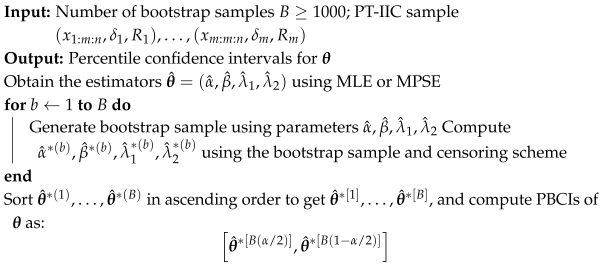
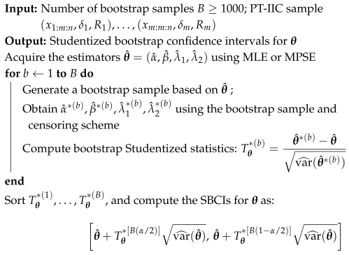
To quantify the theoretical uncertainty of the point estimates, asymptotic confidence intervals rely on the observed Fisher information matrices. These matrices (Equations (6) and (7)) are constructed by taking the negative second partial derivatives of the log-likelihood and log-spacing objective functions. Because the exact analytical derivations are highly complex (as detailed in the Appendix A), this study evaluates these matrices using numerical differentiation to obtain the standard errors. To complement the asymptotic approach, bootstrap resampling techniques are employed; specifically, percentile bootstrap confidence intervals(PBCIs) and Studentized bootstrap confidence intervals (SBCIs) are derived, providing alternative measures of uncertainty that do not rely on asymptotic assumptions. See [42,43] for additional details on this connection. Algorithm 1 details the procedure for generating PBCIs, while Algorithm 2 describes the steps required to acquire SBCIs.

Algorithm 1: Percentile Bootstrap Confidence Intervals (PBCIs)

Algorithm 2: Studentized Bootstrap Confidence Intervals (SBCIs)

5. Monte Carlo Simulation Outcomes

Monte Carlo simulation studies are a cornerstone tool for assessing how well inferential methods, such as estimation techniques, hold up across a range of conditions. Researchers widely rely on them in comparative studies to gauge estimation accuracy, consistency, and efficiency, ultimately producing meaningful numerical benchmarks. A broad body of literature has incorporated Monte Carlo simulation studies, including [44,45,46,47,48,49,50,51,52]. This section presents Monte Carlo simulation results to compare the inferential procedures introduced earlier. All numerical computations were carried out in RStudio (v2025.9.0.387) [53], a popular integrated development environment (IDE) built around R (v4.5.1) [54], a powerful environment for statistical computing, visualization, and data analysis. Since the optimization problems under consideration are nonlinear, the nloptr (v2.2.1) package was used as an R interface to NLopt, a free, open-source library for nonlinear optimization. This framework brings together a unified interface to a wide range of freely available optimization routines, along with native implementations of several algorithms [55]. Of particular note is the Bound Optimization by Quadratic Approximation (BOBYQA) algorithm [56], which proved especially effective in computing the estimators. The calculated optimized objects are approved when the relative change through sequential iterations is less than $1\times {10}^{-12}$ or when the maximum number of evaluations ($1\times {10}^3$) is reached. For each simulation run, the initial parameter values are generated by uniform sampling within $10\%$ of the given parameters. Furthermore, if either of the two estimation objects fails in convergence, new initial values are generated until the convergence criteria are satisfied. To evaluate the estimator’s performance under a range of situations, including different tail behaviors and skewness levels, various combinations of shape parameters are selected above and below 1. Simultaneously, the variation in the scale parameters facilitates evaluation of scale invariance across different data dispersions. Without loss of generality, different sample sizes (n), effective observed sample sizes (m), sampling schemes, and model parameters are considered.

The Monte Carlo simulation was designed to evaluate the estimators across a comprehensive grid of scenarios, assessing performance against varying hazard shapes, censoring severities, and dropout timings. To ensure numerical stability and adequate convergence across the nonlinear optimization routines, the study utilizes $N=1000$ Monte Carlo replications and $B=1000$ bootstrap samples per configuration. To thoroughly evaluate the impact of information loss, the simulation covers a wide range of censoring proportions and timing (detailed in Table 1). The schemes represent varied experimental conditions. For instance, Scheme 2 (50% loss) and Scheme 3 (62.5% loss) represent heavy censoring, while Scheme 1 (20% loss) and Schemes 4–7 (25% loss) represent light censoring. For some censoring levels, different removal patterns were tested to assess the impact of dropout timing. The true parameter values (detailed in Table 2) were not chosen arbitrarily. The shape parameters ($\alpha$ and $\beta$) were selected to evaluate the model across the distinct hazard-rate profiles characteristic of the generalized gamma distribution (e.g., decreasing, increasing, and bathtub-shaped hazards) by alternating between values above and below 1. Simultaneously, the scale parameters (${\lambda }_1,{\lambda }_2$) were selected to test the estimators’ scale invariance. By shifting ${\lambda }_2$ from 2.5 to 5.0 while holding ${\lambda }_1$ constant, we conducted a built-in sensitivity analysis to evaluate cross-parameter interference and assess how differing risk magnitudes affect estimation variance (For the sake of conciseness, simulation outcomes of the first two cases are reported here. The remaining results are available upon request from the corresponding author.).

Table 1. Utilized sample sizes (n), effective sample sizes (m), and progressive censoring schemes.

Scheme	n	m	Removal Scheme (R)
$\left[1\right]$	15	12	$R_1=\cdots =R_{11}=0,R_{12}=3$
$\left[2\right]$	30	15	$R_1=\cdots =R_{14}=0,R_{15}=15$
$\left[3\right]$	40	15	$R_1=\cdots =R_{14}=0,R_{15}=25$
$\left[4\right]$	40	30	$R_1=\cdots =R_{29}=0,R_{30}=10$
$\left[5\right]$	40	30	$R_2=\cdots =R_{30}=0,R_1=10$
$\left[6\right]$	40	30	$R_2=\cdots =R_{29}=0,R_1=R_{30}=5$
$\left[7\right]$	40	30	$R_1=\cdots =R_{14}=R_{17}=\cdots =R_{30}=0,R_{15}=R_{16}=5$

Table 2. Cases of model parameters considered for the Monte Carlo simulation study.

Case	$\mathit{\alpha }$	$\mathit{\beta }$	${\mathit{\lambda }}_1$	${\mathit{\lambda }}_2$
1	2	0.75	2	2.5
2	2	0.75	1.25	5
3	2	3	2	2.5
4	2	3	1.25	5
5	0.5	0.75	2	2.5
6	0.5	0.75	1.25	5
7	0.5	3	2	2.5
8	0.5	3	1.25	5

The conducted Monte Carlo simulation study reported in this article comprises two distinct parts. The first part evaluates the efficiency of point estimators using the root-mean-square error (RMSE), while interval estimators are assessed by their simulated average lengths and the coverage probabilities of confidence intervals under both MLEs and MPSEs. For a given simulation run (i), where ${\widehat{\theta }}_i$ denotes the point estimator of $\theta$, the simulated RMSE is computed as follows:

$$\mathrm{RMSE}\left(\widehat{\theta }\right)=\sqrt{{\displaystyle \frac{1}{N}}{\displaystyle \sum _{i=1}^N}{({\widehat{\theta }}_i-\theta )}^2}.$$

A low RMSE, short average lengths, and coverage probabilities close to unity indicate good performance. The second part assesses the goodness of fit in terms of the average absolute difference ($D_{\mathrm{abs}}$) between the true and estimated CDFs and the maximum absolute difference ($D_{\max }$) between the true and estimated CDFs to evaluate the estimation methodologies. These metrics are defined as

$$D_{\mathrm{abs}}={\displaystyle \frac{1}{n\times N}}{\displaystyle \sum _{i=1}^N}{\displaystyle \sum _{j=1}^n}\left|F(x_j;\mathit{\theta })-F(x_j;\widehat{{\mathit{\theta }}_i})\right|,$$

and

$$D_{\max }={\displaystyle \frac{1}{N}}{\displaystyle \sum _{i=1}^N}\underset{j=1,..,n}{\max }\left|F(x_j;\mathit{\theta })-F(x_j;\widehat{{\mathit{\theta }}_i})\right|,$$

where ${\widehat{\mathit{\theta }}}_i$ represents the estimated model parameters of the model parameter ($\mathit{\theta }$) obtained from simulation run i. Values of $D_{\mathrm{abs}}$ and $D_{\max }$ close to 0 indicate that the fitted model is suitable for the data.

Table 3 shows the simulated biases and RMSEs (within parentheses) under different simulation settings for the considered point estimators (i.e., the MLEs and the MPSEs). The simulation results reveal several important differences in estimation efficiency between the two methods. To begin with, consistent with standard asymptotic theory, the average bias and MSE values for all estimators tend to shrink as the sample size (n) and the effective sample size (m) increase or as the censoring proportion decreases. This behavior confirms the asymptotic consistency of both MLE and MPSE for the proposed model. A standout observation is that MPSEs outperformed MLE in estimating the shape parameter ($\beta$), resulting in noticeably lower average bias and tighter MSEs across nearly all considered schemes and parameter settings. Looking at the direction of bias, MLE tends to overestimate the $\alpha$ parameter, whereas MPSE generally underestimates it. Overall, MPSEs often match or exceed MLEs in terms of MSE for $\alpha$, especially under heavier censoring or smaller effective sample sizes (e.g., Schemes 1 and 2), suggesting greater statistical stability when available information is scarce. Increasing the value of ${\lambda }_2$ relative to ${\lambda }_1$ generally elevates the mean squared error for ${\widehat{\lambda }}_2$, whether MLEs and MPSEs are considered, indicating that larger scale parameters exhibit higher estimation variance for a fixed effective sample size (m). This shift also induces minor cross-parameter sensitivity, slightly inflating the MSEs for the shape parameter ($\beta$). In general, the simulation results indicate that MPSEs are strong and reliable alternatives to MLEs.

Table 3. Simulated biased and RMSEs (within parentheses) assuming different censoring schemes, estimation methods, and model parameters.

Scheme	Method	Model Parameters	$\widehat{\mathit{\alpha }}$	$\widehat{\mathit{\beta }}$	${\widehat{\mathit{\lambda }}}_1$	${\widehat{\mathit{\lambda }}}_2$
$\left[1\right]$	MLE	(2, 0.75, 2, 2.5)	0.367 (0.935)	0.163 (0.364)	0.550 (1.126)	0.611 (1.265)
		(2, 0.75, 1.25, 5)	0.351 (0.900)	0.232 (0.618)	0.521 (1.001)	0.720 (3.866)
	MPSE	(2, 0.75, 2, 2.5)	−0.285 (0.653)	−0.019 (0.227)	0.683 (1.274)	0.939 (1.694)
		(2, 0.75, 1.25, 5)	−0.247 (0.597)	0.030 (0.345)	0.443 (0.877)	1.848 (4.786)
$\left[2\right]$	MLE	(2, 0.75, 2, 2.5)	0.311 (0.744)	0.153 (0.264)	0.446 (0.793)	0.567 (1.117)
		(2, 0.75, 1.25, 5)	0.307 (0.709)	0.188 (0.462)	0.347 (0.586)	0.437 (2.519)
	MPSE	(2, 0.75, 2, 2.5)	−0.229 (0.520)	−0.011 (0.169)	0.575 (0.999)	0.886 (1.507)
		(2, 0.75, 1.25, 5)	−0.177 (0.485)	0.015 (0.176)	0.315 (0.592)	1.586 (3.616)
$\left[3\right]$	MLE	(2, 0.75, 2, 2.5)	0.381 (0.825)	0.159 (0.262)	0.389 (0.784)	0.452 (1.065)
		(2, 0.75, 1.25, 5)	0.361 (0.769)	0.189 (0.319)	0.312 (0.511)	0.117 (2.246)
	MPSE	(2, 0.75, 2, 2.5)	−0.185 (0.528)	−0.007 (0.183)	0.573 (1.040)	0.827 (1.486)
		(2, 0.75, 1.25, 5)	−0.150 (0.484)	0.031 (0.204)	0.355 (0.609)	1.453 (3.198)
$\left[4\right]$	MLE	(2, 0.75, 2, 2.5)	0.116 (0.398)	0.105 (0.163)	0.501 (0.738)	0.592 (0.948)
		(2, 0.75, 1.25, 5)	0.112 (0.389)	0.100 (0.181)	0.303 (0.513)	1.117 (2.446)
	MPSE	(2, 0.75, 2, 2.5)	−0.172 (0.363)	0.019 (0.138)	0.489 (0.820)	0.645 (1.084)
		(2, 0.75, 1.25, 5)	−0.151 (0.340)	0.022 (0.121)	0.262 (0.495)	1.663 (3.007)
$\left[5\right]$	MLE	(2, 0.75, 2, 2.5)	0.036 (0.313)	0.084 (0.204)	0.481 (0.827)	0.647 (1.115)
		(2, 0.75, 1.25, 5)	0.072 (0.348)	0.085 (0.171)	0.322 (0.634)	1.215 (2.599)
	MPSE	(2, 0.75, 2, 2.5)	−0.243 (0.368)	−0.009 (0.100)	0.436 (0.789)	0.653 (1.120)
		(2, 0.75, 1.25, 5)	−0.197 (0.349)	0.004 (0.128)	0.267 (0.637)	1.648 (3.229)
$\left[6\right]$	MLE	(2, 0.75, 2, 2.5)	0.081 (0.360)	0.099 (0.171)	0.503 (0.760)	0.629 (1.004)
		(2, 0.75, 1.25, 5)	0.070 (0.343)	0.091 (0.163)	0.324 (0.568)	1.289 (2.679)
	MPSE	(2, 0.75, 2, 2.5)	−0.199 (0.354)	0.008 (0.108)	0.461 (0.756)	0.653 (1.073)
		(2, 0.75, 1.25, 5)	−0.181 (0.342)	0.014 (0.109)	0.271 (0.514)	1.783 (3.061)
$\left[7\right]$	MLE	(2, 0.75, 2, 2.5)	0.053 (0.320)	0.089 (0.149)	0.469 (0.734)	0.608 (0.991)
		(2, 0.75, 1.25, 5)	0.066 (0.320)	0.092 (0.158)	0.330 (0.593)	1.313 (2.725)
	MPSE	(2, 0.75, 2, 2.5)	−0.230 (0.364)	-0.006 (0.103)	0.437 (0.771)	0.652 (1.112)
		(2, 0.75, 1.25, 5)	−0.199 (0.332)	0.006 (0.132)	0.263 (0.531)	1.779 (3.218)

Table 4 compares the simulated coverage probabilities at 90% and 95% confidence levels across the previously mentioned CIs—ACIs, PBCIs, and SBCIs—without loss of generality. A closer look at the simulation results reveals a clear ranking of interval performance. Among the three, ACI consistently achieves the highest coverage probabilities across all model parameters, censoring schemes, and estimators (MLEs and MPSEs). In nearly every examined scenario, ACI coverage meets or slightly exceeds the nominal confidence levels. Although values near 1.00 indicate that these intervals are conservative and likely wider, they provide strong assurance that the true parameter value is captured. On the other hand, PBCI frequently falls short, exhibiting notable under-coverage, especially for the shape parameter ($\beta$) and the scale parameters (${\lambda }_1$, ${\lambda }_2$), and failing to reach nominal levels in most schemes. SBCI, however, marks a meaningful step up from the standard percentile approach. Furthermore, evaluating the coverage probabilities under the two considered parameter cases reveals the sensitivity of the interval estimation methods to the distribution’s underlying scale parameters. The ACIs remain largely impervious to this parameter shift, consistently maintaining near-perfect albeit highly conservative coverage probabilities approaching 1 across both configurations. Conversely, the resampling-based intervals, particularly the PBCIs and SBCIs, exhibit noticeable degradation in coverage for the scale parameters when ${\lambda }_2$ is increased from 2.5 to 5. This behavior aligns with the previously observed point-estimation properties—namely, a larger true value of ${\lambda }_2$ induces greater estimation variance. Consequently, the PBCI and SBCI coverage probabilities for ${\lambda }_2$ are pulled further below their nominal 90% and 95% targets in the second case. Importantly, the coverage probabilities for the shape parameters ($\alpha$ and $\beta$) remain comparatively stable across the two cases, confirming that the bootstrap methods are primarily sensitive to variation driven by changes in the scale parameters. Overall, under regularity conditions, ACIs should be considered for applications in which meeting the nominal coverage level is essential, while SBCI is the better resampling-based option when finite-sample behavior makes asymptotic normality assumptions less reliable. Moreover, MLEs generally outperform MPSEs in terms of coverage probability across these simulations. MLEs maintain more stable coverage across bootstrap intervals (i.e., PBCIs and SBCIs), whereas MPSEs often perform noticeably worsethan the MLEs.

Table 4. Simulated coverage probabilities of ACIs, PBCIs, and SBCIs under different simulation settings.

Scheme	Method	Model Parameters	CI Type	$\mathit{\alpha }$		$\mathit{\beta }$		${\mathit{\lambda }}_1$		${\mathit{\lambda }}_2$
				90%	95%	90%	95%	90%	95%	90%	5%
$\left[1\right]$	MLE	(2, 0.75, 2, 2.5)	ACI	0.991	0.994	1.000	1.000	1.000	0.993	0.993	0.996
			PBCI	0.790	0.844	0.525	0.635	0.613	0.824	0.714	0.929
			SBCI	0.850	0.926	0.629	0.808	0.813	0.950	0.885	0.965
		(2, 0.75, 1.25, 5)	ACI	0.997	0.999	1.000	1.000	1.000	0.999	0.999	1.000
			PBCI	0.789	0.834	0.514	0.672	0.600	0.802	0.696	0.861
			SBCI	0.843	0.932	0.630	0.812	0.792	0.929	0.867	0.957
	MPSE	(2, 0.75, 2, 2.5)	ACI	0.990	0.995	1.000	1.000	1.000	0.999	0.999	0.999
			PBCI	0.730	0.794	0.554	0.709	0.724	0.883	0.783	0.935
			SBCI	0.800	0.920	0.612	0.817	0.881	0.950	0.910	0.959
		(2, 0.75, 1.25, 5)	ACI	0.996	0.998	1.000	1.000	1.000	1.000	1.000	1.000
			PBCI	0.869	0.923	0.495	0.610	0.324	0.436	0.376	0.481
			SBCI	0.862	0.927	0.620	0.768	0.390	0.557	0.457	0.630
$\left[2\right]$	MLE	(2, 0.75, 2, 2.5)	ACI	0.995	0.997	1.000	1.000	1.000	0.997	0.997	0.999
			PBCI	0.889	0.948	0.557	0.659	0.408	0.516	0.404	0.513
			SBCI	0.860	0.926	0.645	0.772	0.458	0.625	0.486	0.648
		(2, 0.75, 1.25, 5)	ACI	0.995	0.998	1.000	1.000	1.000	0.999	0.999	0.999
			PBCI	0.890	0.941	0.530	0.628	0.332	0.443	0.375	0.477
			SBCI	0.866	0.916	0.651	0.792	0.393	0.575	0.438	0.602
	MPSE	(2, 0.75, 2, 2.5)	ACI	0.998	0.999	1.000	1.000	1.000	1.000	1.000	1.000
			PBCI	0.885	0.935	0.524	0.607	0.385	0.506	0.408	0.530
			SBCI	0.861	0.928	0.594	0.733	0.439	0.597	0.475	0.648
		(2, 0.75, 1.25, 5)	ACI	0.989	0.994	1.000	1.000	1.000	0.986	1.000	1.000
			PBCI	0.800	0.858	0.473	0.622	0.420	0.695	0.867	0.919
			SBCI	0.883	0.948	0.620	0.841	0.549	0.863	0.861	0.908
$\left[3\right]$	MLE	(2, 0.75, 2, 2.5)	ACI	0.994	0.997	1.000	1.000	1.000	0.992	0.998	0.999
			PBCI	0.788	0.841	0.507	0.668	0.379	0.619	0.875	0.910
			SBCI	0.859	0.934	0.605	0.828	0.502	0.775	0.863	0.903
		(2, 0.75, 1.25, 5)	ACI	0.993	0.997	1.000	1.000	1.000	0.996	0.999	0.999
			PBCI	0.740	0.813	0.502	0.661	0.465	0.715	0.845	0.884
			SBCI	0.846	0.943	0.596	0.806	0.621	0.876	0.838	0.885
	MPSE	(2, 0.75, 2, 2.5)	ACI	0.995	0.998	0.999	1.000	0.999	0.999	0.998	1.000
			PBCI	0.864	0.920	0.526	0.636	0.319	0.504	0.814	0.941
			SBCI	0.857	0.927	0.616	0.790	0.363	0.607	0.925	0.967
		(2, 0.75, 1.25, 5)	ACI	0.996	0.997	1.000	1.000	1.000	0.996	0.997	0.999
			PBCI	0.888	0.951	0.568	0.687	0.428	0.616	0.764	0.926
			SBCI	0.875	0.923	0.647	0.794	0.466	0.709	0.907	0.968
$\left[4\right]$	MLE	(2, 0.75, 2, 2.5)	ACI	0.990	0.995	0.999	1.000	0.999	0.998	1.000	1.000
			PBCI	0.895	0.943	0.546	0.656	0.363	0.534	0.779	0.931
			SBCI	0.893	0.943	0.634	0.793	0.417	0.626	0.923	0.976
		(2, 0.75, 1.25, 5)	ACI	0.996	0.998	1.000	1.000	1.000	1.000	1.000	1.000
			PBCI	0.899	0.946	0.554	0.675	0.390	0.593	0.751	0.932
			SBCI	0.888	0.942	0.636	0.801	0.441	0.695	0.913	0.975
	MPSE	(2, 0.75, 2, 2.5)	ACI	0.912	0.948	0.999	0.999	0.999	0.998	0.998	0.999
			PBCI	0.570	0.701	0.834	0.922	0.701	0.857	0.673	0.855
			SBCI	0.476	0.552	0.728	0.806	0.835	0.936	0.828	0.949
		(2, 0.75, 1.25, 5)	ACI	0.926	0.960	0.999	0.999	0.999	1.000	1.000	1.000
			PBCI	0.638	0.760	0.872	0.911	0.640	0.790	0.596	0.731
			SBCI	0.553	0.626	0.780	0.824	0.796	0.930	0.757	0.918
$\left[5\right]$	MLE	(2, 0.75, 2, 2.5)	ACI	0.915	0.944	0.994	0.995	0.994	1.000	0.999	0.999
			PBCI	0.674	0.795	0.853	0.902	0.664	0.810	0.635	0.777
			SBCI	0.612	0.670	0.780	0.821	0.829	0.943	0.816	0.942
		(2, 0.75, 1.25, 5)	ACI	0.965	0.978	0.999	1.000	0.999	0.999	0.999	0.999
			PBCI	0.597	0.703	0.879	0.934	0.496	0.616	0.473	0.568
			SBCI	0.524	0.615	0.840	0.892	0.578	0.745	0.545	0.704
	MPSE	(2, 0.75, 2, 2.5)	ACI	0.955	0.978	0.999	1.000	0.999	0.999	0.999	0.999
			PBCI	0.424	0.554	0.881	0.938	0.567	0.670	0.502	0.610
			SBCI	0.399	0.486	0.815	0.883	0.632	0.792	0.585	0.738
		(2, 0.75, 1.25, 5)	ACI	0.962	0.977	1.000	1.000	1.000	1.000	1.000	1.000
			PBCI	0.540	0.669	0.894	0.956	0.526	0.641	0.493	0.597
			SBCI	0.483	0.569	0.844	0.889	0.606	0.767	0.564	0.722
$\left[6\right]$	MLE	(2, 0.75, 2, 2.5)	ACI	0.951	0.977	0.999	0.999	0.999	0.999	1.000	1.000
			PBCI	0.423	0.555	0.874	0.935	0.554	0.673	0.487	0.591
			SBCI	0.405	0.497	0.807	0.857	0.616	0.773	0.552	0.710
		(2, 0.75, 1.25, 5)	ACI	0.943	0.971	0.999	1.000	0.999	0.994	0.998	1.000
			PBCI	0.610	0.777	0.885	0.946	0.696	0.894	0.932	0.964
			SBCI	0.486	0.561	0.814	0.865	0.804	0.933	0.934	0.958
	MPSE	(2, 0.75, 2, 2.5)	ACI	0.938	0.960	0.996	0.999	0.996	0.999	1.000	1.000
			PBCI	0.689	0.842	0.902	0.943	0.685	0.872	0.919	0.975
			SBCI	0.589	0.671	0.824	0.861	0.795	0.936	0.951	0.963
		(2, 0.75, 1.25, 5)	ACI	0.927	0.957	0.996	0.997	0.996	1.000	1.000	1.000
			PBCI	0.743	0.837	0.898	0.956	0.686	0.885	0.942	0.979
			SBCI	0.633	0.695	0.844	0.878	0.813	0.938	0.950	0.964
$\left[7\right]$	MLE	(2, 0.75, 2, 2.5)	ACI	0.974	0.985	1.000	1.000	1.000	1.000	0.999	1.000
			PBCI	0.636	0.764	0.879	0.948	0.561	0.727	0.587	0.738
			SBCI	0.562	0.654	0.873	0.914	0.619	0.805	0.754	0.922
		(2, 0.75, 1.25, 5)	ACI	0.969	0.985	1.000	1.000	1.000	0.997	0.999	1.000
			PBCI	0.497	0.642	0.891	0.944	0.646	0.768	0.598	0.752
			SBCI	0.455	0.557	0.857	0.903	0.692	0.842	0.765	0.912
	MPSE	(2, 0.75, 2, 2.5)	ACI	0.969	0.983	0.999	0.999	0.999	1.000	1.000	1.000
			PBCI	0.584	0.707	0.896	0.947	0.600	0.755	0.566	0.699
			SBCI	0.524	0.614	0.878	0.916	0.648	0.854	0.723	0.893
		(2, 0.75, 1.25, 5)	ACI	0.967	0.986	1.000	1.000	1.000	0.999	1.000	1.000
			PBCI	0.489	0.648	0.896	0.943	0.648	0.766	0.559	0.710
			SBCI	0.459	0.549	0.864	0.914	0.707	0.848	0.729	0.908

Table 5 summarizes the simulated average lengths of the CIs. Clearly, ACIs yield lengths that are drastically wider (often spanning large units for ${\lambda }_1$ and ${\lambda }_2$), which fully explains their near-unity coverage. On the contrary, PBCIs are noticeably the tightest, resulting in the previously observed under-coverage penalty. The SBCIs serve as an effective compromise, being slightly wider than the PBCIs to correct coverage probabilities without pushing them to the extremes of the ACIs. Consistent with the point-estimation results, increasing the true value of ${\lambda }_2$ from 2.5 to 5 generally increases the average lengths of the corresponding confidence intervals across all considered methods. This widening is a direct theoretical consequence of the higher estimation-variance MSEs associated with the larger scale parameter, forcing both the asymptotic and bootstrap methods to generate broader bounds to try to capture the true value. Conversely, the interval lengths for the shape parameters ($\alpha$ and $\beta$) remain relatively stable between the two cases. Overall, MPSEs generally outperform MLE in terms of interval length, consistently producing narrower confidence bounds across most schemes and interval types. However, while these tighter intervals indicate higher precision for MPSEs, they also directly account for their higher rate of under-coverage observed in the bootstrap intervals compared to the wider, more conservative MLEs.

Table 5. Simulated average lengths of the ACIs, PBCIs, and SBCIs under different settings.

Scheme	Method	Model Parameters	CI Type	$\mathit{\alpha }$		$\mathit{\beta }$		${\mathit{\lambda }}_1$		${\mathit{\lambda }}_2$
				90%	95%	90%	95%	90%	95%	90%	95%
$\left[1\right]$	MLE	(2, 0.75, 2, 2.5)	ACI	8.373	9.977	6.133	7.308	46.723	55.673	57.119	68.062
			PBCI	2.815	3.570	0.871	1.241	2.933	3.973	3.931	5.199
			SBCI	2.725	3.763	0.820	1.185	3.880	7.236	5.263	9.275
		(2, 0.75, 1.25, 5)	ACI	7.497	8.933	7.021	8.367	49.707	59.230	59.220	70.565
			PBCI	2.317	2.921	0.754	0.964	2.298	2.968	3.360	4.287
			SBCI	2.470	3.391	0.923	1.268	3.664	5.426	4.807	6.977
	MPSE	(2, 0.75, 2, 2.5)	ACI	7.675	9.146	7.687	9.160	51.027	60.803	60.893	72.558
			PBCI	2.394	3.026	0.813	1.034	2.225	2.874	3.179	4.054
			SBCI	2.622	3.620	1.057	1.476	3.929	5.815	5.207	7.568
		(2, 0.75, 1.25, 5)	ACI	5.323	6.343	4.380	5.219	35.634	42.461	43.911	52.323
			PBCI	1.215	1.508	0.458	0.542	1.791	2.186	2.462	3.023
			SBCI	1.630	2.156	0.591	0.749	2.385	3.096	3.125	4.021
$\left[2\right]$	MLE	(2, 0.75, 2, 2.5)	ACI	4.154	4.950	2.830	3.372	25.824	30.771	33.014	39.339
			PBCI	1.035	1.287	0.412	0.497	1.894	2.361	2.666	3.338
			SBCI	1.381	1.816	0.434	0.542	2.089	2.748	2.876	3.749
		(2, 0.75, 1.25, 5)	ACI	4.629	5.515	3.600	4.290	30.506	36.350	38.075	45.369
			PBCI	1.141	1.413	0.439	0.523	1.829	2.241	2.531	3.114
			SBCI	1.450	1.908	0.492	0.621	2.148	2.805	2.858	3.676
	MPSE	(2, 0.75, 2, 2.5)	ACI	3.792	4.518	2.722	3.244	23.905	28.485	29.806	35.516
			PBCI	1.031	1.288	0.411	0.491	1.830	2.265	2.567	3.194
			SBCI	1.202	1.582	0.414	0.516	1.920	2.514	2.565	3.319
		(2, 0.75, 1.25, 5)	ACI	8.824	10.515	6.186	7.370	29.584	35.252	96.388	114.854
			PBCI	2.783	3.540	1.348	2.173	1.992	3.071	8.237	11.252
			SBCI	3.080	4.315	1.173	1.737	4.116	11.331	19.570	32.880
$\left[3\right]$	MLE	(2, 0.75, 2, 2.5)	ACI	7.235	8.621	6.365	7.584	27.441	32.698	93.277	111.146
			PBCI	2.268	2.860	0.925	1.278	1.325	1.872	6.684	8.599
			SBCI	2.419	3.304	1.027	1.464	2.271	4.622	14.057	21.114
		(2, 0.75, 1.25, 5)	ACI	7.378	8.791	6.874	8.191	28.132	33.521	92.252	109.925
			PBCI	2.320	2.929	0.959	1.285	1.210	1.663	5.998	7.652
			SBCI	2.492	3.418	1.044	1.485	2.162	3.968	14.030	20.457
	MPSE	(2, 0.75, 2, 2.5)	ACI	4.750	5.661	3.406	4.059	18.314	21.822	71.850	85.614
			PBCI	1.191	1.489	0.471	0.592	1.059	1.415	7.158	8.785
			SBCI	1.529	2.026	0.512	0.667	1.349	1.952	8.788	11.811
		(2, 0.75, 1.25, 5)	ACI	4.347	5.179	2.571	3.063	15.460	18.421	60.886	72.551
			PBCI	1.074	1.344	0.417	0.543	1.192	1.727	7.694	9.726
			SBCI	1.513	2.015	0.451	0.583	1.455	2.190	8.724	12.028
$\left[4\right]$	MLE	(2, 0.75, 2, 2.5)	ACI	4.678	5.574	3.133	3.733	17.837	21.254	70.147	83.585
			PBCI	1.124	1.403	0.445	0.566	1.122	1.534	7.536	9.332
			SBCI	1.541	2.056	0.492	0.636	1.430	2.101	9.087	12.304
		(2, 0.75, 1.25, 5)	ACI	4.068	4.847	2.557	3.046	14.886	17.738	60.951	72.628
			PBCI	1.053	1.319	0.440	0.574	1.156	1.642	7.751	9.691
			SBCI	1.374	1.823	0.457	0.591	1.413	2.145	8.960	12.265
	MPSE	(2, 0.75, 2, 2.5)	ACI	5.414	6.451	4.739	5.646	52.054	62.027	64.784	77.195
			PBCI	1.335	1.685	0.555	0.694	5.043	6.304	6.953	8.678
			SBCI	3.335	4.252	1.004	1.347	5.080	7.916	6.541	10.100
		(2, 0.75, 1.25, 5)	ACI	4.792	5.710	5.401	6.436	51.913	61.858	66.637	79.403
			PBCI	1.271	1.588	0.559	0.667	3.924	4.962	5.787	7.211
			SBCI	3.073	3.916	1.174	1.571	4.205	6.202	5.617	8.052
$\left[5\right]$	MLE	(2, 0.75, 2, 2.5)	ACI	4.856	5.786	5.564	6.630	52.622	62.703	66.390	79.109
			PBCI	1.320	1.649	0.592	0.713	3.860	4.922	5.613	7.021
			SBCI	3.308	4.192	1.299	1.752	4.121	6.056	5.489	7.843
		(2, 0.75, 1.25, 5)	ACI	3.446	4.106	3.145	3.747	30.085	35.849	37.039	44.134
			PBCI	0.885	1.073	0.406	0.463	2.364	2.985	3.361	4.192
			SBCI	1.759	2.228	0.567	0.725	2.381	3.150	3.103	4.011
	MPSE	(2, 0.75, 2, 2.5)	ACI	3.124	3.723	2.276	2.712	24.825	29.581	32.150	38.310
			PBCI	0.769	0.932	0.326	0.379	2.483	3.162	3.600	4.495
			SBCI	1.603	2.020	0.424	0.532	2.322	3.062	3.220	4.153
		(2, 0.75, 1.25, 5)	ACI	3.208	3.823	2.691	3.206	26.656	31.763	33.889	40.381
			PBCI	0.840	1.017	0.372	0.427	2.359	2.999	3.408	4.267
			SBCI	1.618	2.047	0.477	0.603	2.194	2.903	2.989	3.867
$\left[6\right]$	MLE	(2, 0.75, 2, 2.5)	ACI	3.116	3.713	2.407	2.868	25.040	29.837	31.790	37.880
			PBCI	0.759	0.920	0.344	0.398	2.412	3.068	3.540	4.411
			SBCI	1.572	1.983	0.458	0.577	2.250	2.959	3.069	3.960
		(2, 0.75, 1.25, 5)	ACI	5.074	6.046	4.212	5.019	27.162	32.366	106.931	127.417
			PBCI	1.342	1.707	0.741	1.059	2.786	3.709	15.837	20.913
			SBCI	3.101	4.000	1.018	1.431	3.205	5.994	17.636	27.170
	MPSE	(2, 0.75, 2, 2.5)	ACI	5.196	6.192	5.117	6.097	29.527	35.184	114.896	136.907
			PBCI	1.280	1.608	0.624	0.795	1.937	2.584	12.262	15.501
			SBCI	3.128	4.042	1.177	1.632	2.587	4.384	15.730	23.091
		(2, 0.75, 1.25, 5)	ACI	4.645	5.535	5.231	6.234	29.016	34.575	110.448	131.607
			PBCI	1.314	1.652	0.687	0.871	1.872	2.494	11.574	14.484
			SBCI	2.893	3.725	1.276	1.788	2.435	4.039	15.230	21.996
$\left[7\right]$	MLE	(2, 0.75, 2, 2.5)	ACI	3.203	3.816	2.580	3.074	15.444	18.402	64.935	77.375
			PBCI	0.872	1.064	0.401	0.477	1.259	1.693	9.621	11.867
			SBCI	1.574	2.013	0.509	0.663	1.328	1.910	8.196	10.826
		(2, 0.75, 1.25, 5)	ACI	3.018	3.596	1.980	2.359	13.291	15.837	57.418	68.417
			PBCI	0.781	0.952	0.343	0.412	1.405	1.904	9.924	12.092
			SBCI	1.513	1.918	0.423	0.542	1.381	1.940	8.356	11.010
	MPSE	(2, 0.75, 2, 2.5)	ACI	3.095	3.688	2.312	2.755	14.477	17.250	63.368	75.507
			PBCI	0.833	1.017	0.375	0.449	1.318	1.802	9.987	12.318
			SBCI	1.521	1.947	0.459	0.594	1.331	1.924	8.530	11.312
		(2, 0.75, 1.25, 5)	ACI	3.115	3.711	2.129	2.537	14.064	16.759	61.337	73.088
			PBCI	0.761	0.931	0.358	0.429	1.339	1.823	10.050	12.238
			SBCI	1.545	1.954	0.465	0.594	1.402	1.984	8.644	11.384

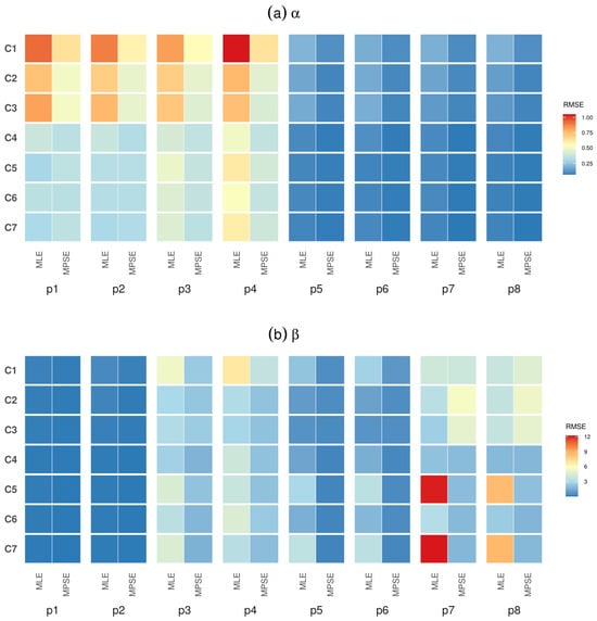
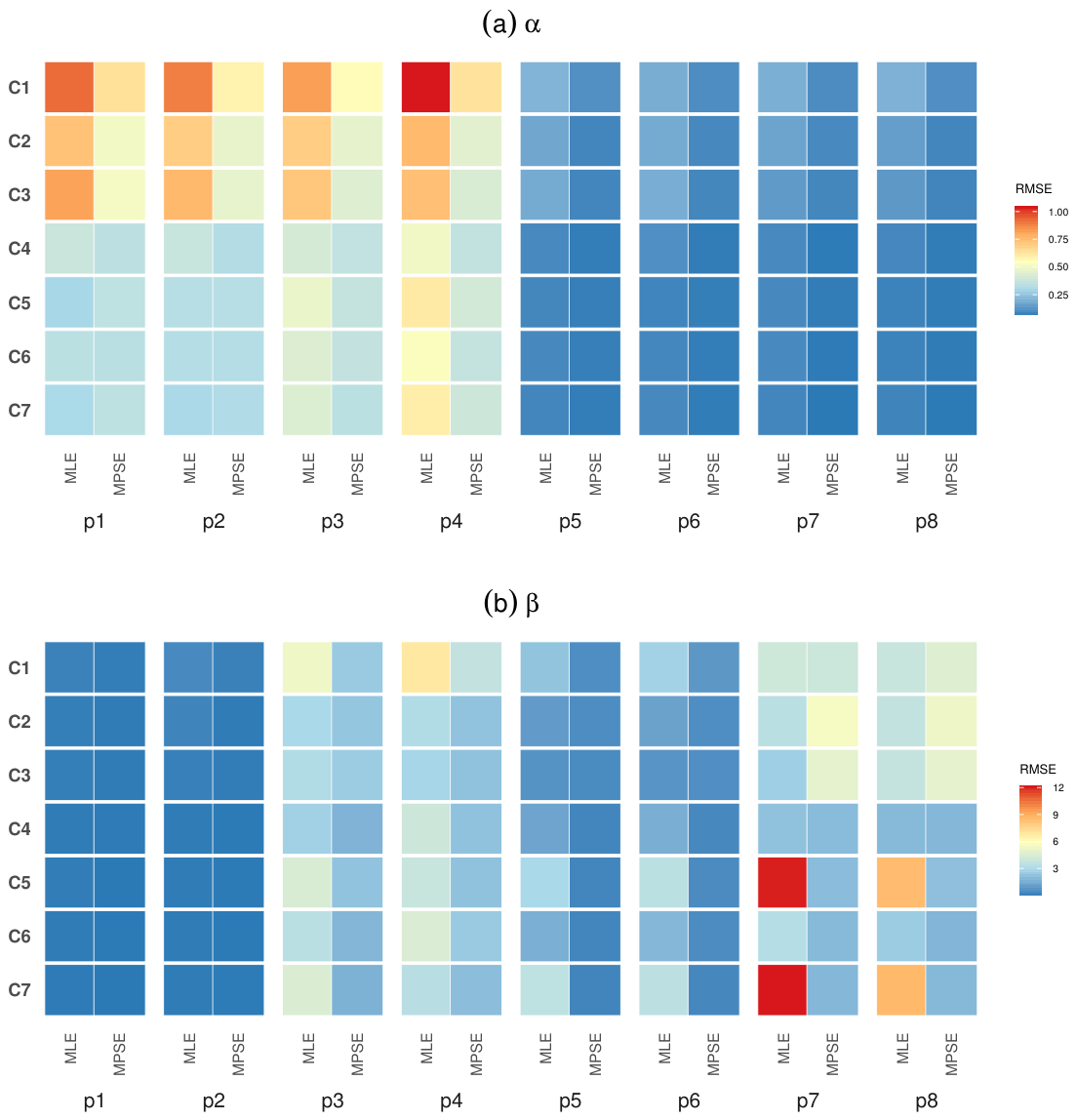
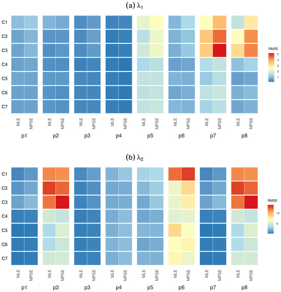
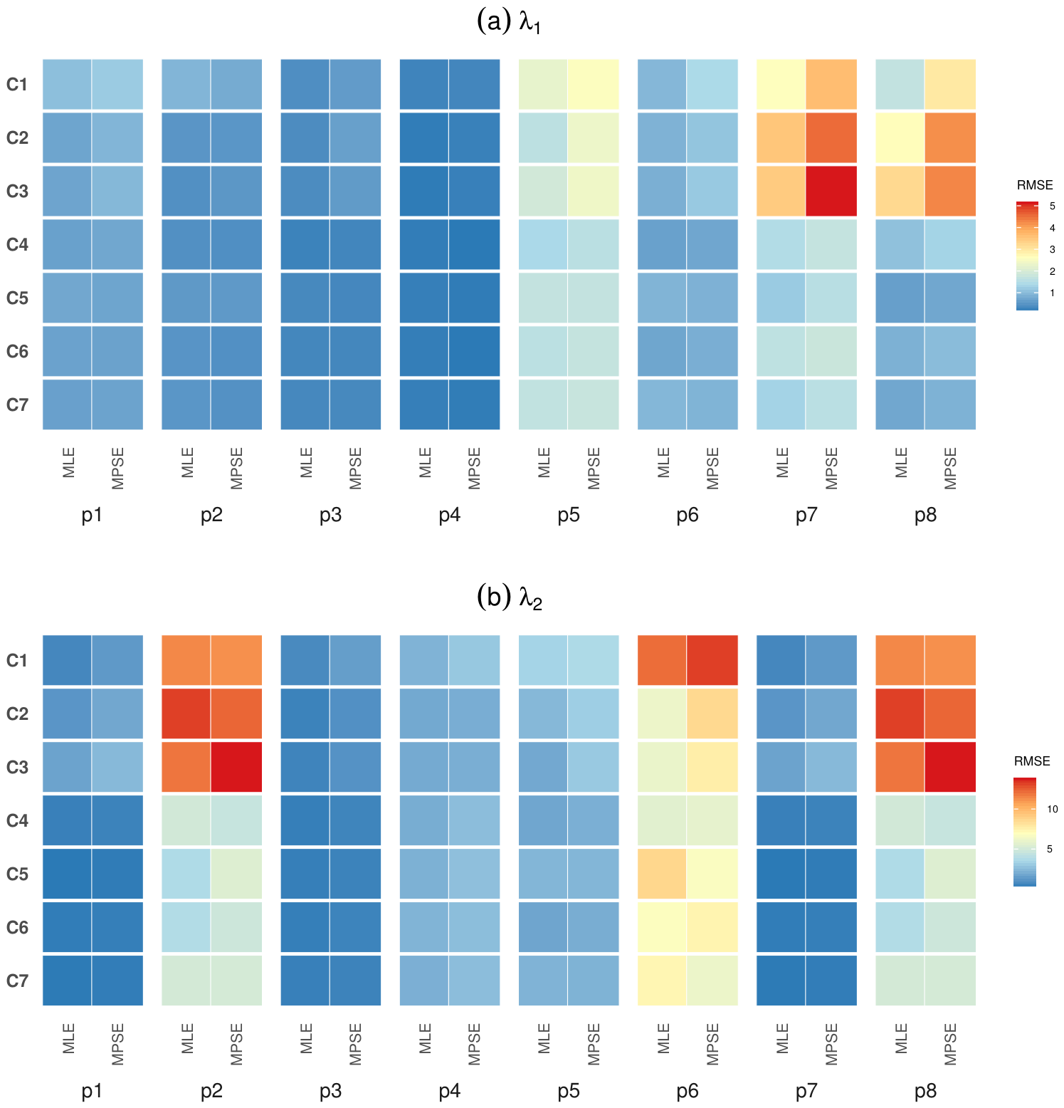
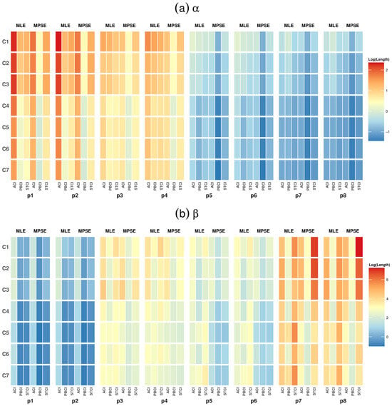
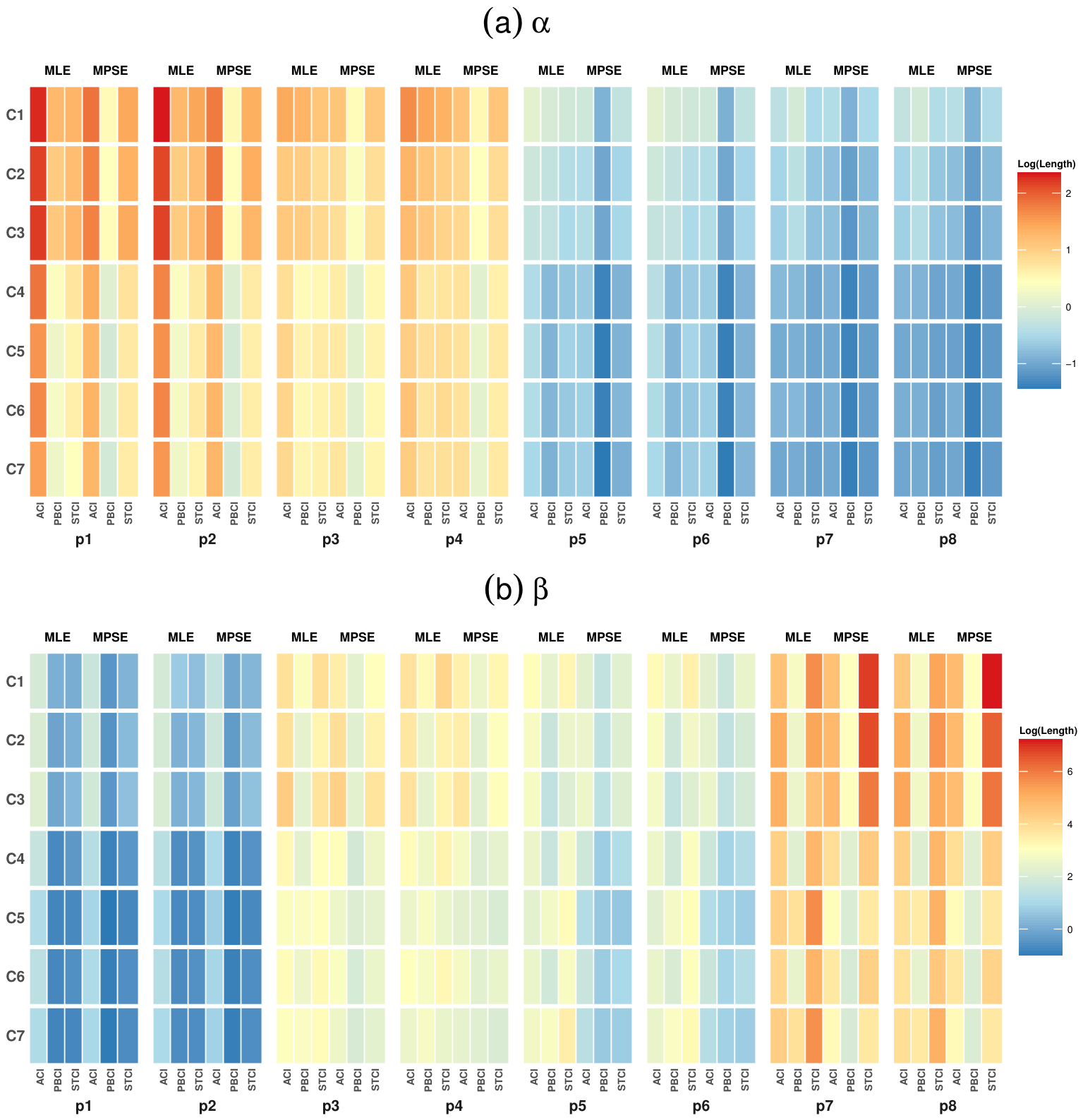
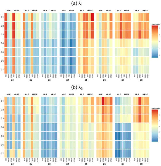
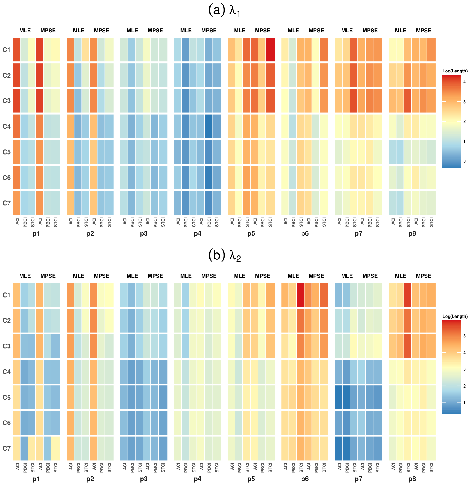
Regarding goodness of fit, Table 6 presents results for the fitted model based on the proposed estimation methods across various simulation settings. Across all considered progressive Type-II censoring schemes, both distance metrics remain notably small. The $D_{\mathrm{abs}}$ values largely range between 0.04 and 0.05, while the $D_{\max }$ values, which bear a conceptual resemblance to the Kolmogorov–Smirnov test statistic, infrequently surpass 0.08, reflecting a very close fit to the true distribution. For a highly flexible four-parameter competing-risks model, achieving this level of closeness to the true CDF is of considerable importance. These small deviations confirm that both MLEs and MPSEs reliably capture the underlying probability distribution, providing the statistical soundness needed for demanding applications in materials science and physical reliability modeling. Both methods perform well overall, though MPSEs consistently deliver competitive results and, at times, outperform MLEs on distance metrics, further establishing their value as an effective estimation approach under progressive censoring. Despite the increased variability in isolated parameter estimates when increasing the value of ${\lambda }_2$ relative to ${\lambda }_1$, the overall goodness-of-fit remains unaffected. The $D_{\mathrm{abs}}$ and $D_{\max }$ metrics stay remarkably low and stable across both parameter sets. The simulation results based on the eight cases of model parameters and seven different schemes for RMSE and the length of CIs (the logarithmic transformation was used to facilitate visual comparison) are given in Figure 1, Figure 2, Figure 3 and Figure 4.

Table 6. Simulated average absolute difference ($D_{\mathrm{abs}}$) and maximum absolute difference ($D_{\max }$) between the true and estimated CDFs under different simulation settings.

Scheme	Method	Model Parameters	${\mathit{D}}_{\mathbf{abs}}$	${\mathit{D}}_{\mathbf{max}}$
$\left[1\right]$	MLE	(2, 0.75, 2, 2.5)	0.073	0.118
		(2, 0.75, 1.25, 5)	0.050	0.082
	MPSE	(2, 0.75, 2, 2.5)	0.042	0.069
		(2, 0.75, 1.25, 5)	0.046	0.075
$\left[2\right]$	MLE	(2, 0.75, 2, 2.5)	0.045	0.073
		(2, 0.75, 1.25, 5)	0.045	0.072
	MPSE	(2, 0.75, 2, 2.5)	0.043	0.074
		(2, 0.75, 1.25, 5)	0.072	0.118
$\left[3\right]$	MLE	(2, 0.75, 2, 2.5)	0.049	0.083
		(2, 0.75, 1.25, 5)	0.042	0.070
	MPSE	(2, 0.75, 2, 2.5)	0.044	0.072
		(2, 0.75, 1.25, 5)	0.046	0.074
$\left[4\right]$	MLE	(2, 0.75, 2, 2.5)	0.046	0.073
		(2, 0.75, 1.25, 5)	0.043	0.073
	MPSE	(2, 0.75, 2, 2.5)	0.076	0.116
		(2, 0.75, 1.25, 5)	0.052	0.082
$\left[5\right]$	MLE	(2, 0.75, 2, 2.5)	0.041	0.067
		(2, 0.75, 1.25, 5)	0.047	0.073
	MPSE	(2, 0.75, 2, 2.5)	0.048	0.076
		(2, 0.75, 1.25, 5)	0.047	0.072
$\left[6\right]$	MLE	(2, 0.75, 2, 2.5)	0.046	0.075
		(2, 0.75, 1.25, 5)	0.074	0.110
	MPSE	(2, 0.75, 2, 2.5)	0.050	0.079
		(2, 0.75, 1.25, 5)	0.042	0.066
$\left[7\right]$	MLE	(2, 0.75, 2, 2.5)	0.045	0.069
		(2, 0.75, 1.25, 5)	0.047	0.073
	MPSE	(2, 0.75, 2, 2.5)	0.047	0.071
		(2, 0.75, 1.25, 5)	0.044	0.072

Figure 1. Heatmap plot of the simulated RMSE of shape parameters $\alpha$ and $\beta$ based on the eight cases of model parameters (P) and seven different schemes (C). Red color indicates high RMSEs while blue color indicates low RMSEs.

Figure 2. Heatmap plot of the simulated RMSE of scale parameters ${\lambda }_1$ and ${\lambda }_2$ based on the eight cases of model parameters (P) and seven different schemes (C). Red color indicates high RMSEs, while blue color indicates low RMSEs.

Figure 3. Heatmap plot of the log length of ACIs, PBCIs, and SBCIs at the 95% significance level for shape parameters $\alpha$ and $\beta$ based on the eight cases of model parameters (P) and seven different schemes (C).

Figure 4. Heatmap plot of the log length of ACIs, PBCIs, and SBCIs at the 95% significance level for scale parameters ${\lambda }_1$ and ${\lambda }_2$ based on the eight cases of model parameters (P) and seven different schemes (C).

Before concluding this section, it is important to fully interpret these interval dynamics, that is, it is crucial to understand why the PBCI frequently under-covers. The PBCI fundamentally assumes that the sampling distribution of the parameter estimators is symmetric. However, under heavy progressive censoring (the effective sample size (m) is much smaller than n), the sampling distributions for the scale and shape parameters become highly skewed due to information loss. Because PBCI does not correct for this skewness, its symmetric bounds fail to capture the true parameter value. The SBCI mitigates this by standardizing the bootstrap statistic using its estimated variance, thereby achieving second-order asymptotic accuracy and successfully correcting for skewness. Furthermore, the censoring level directly dictates this performance trade-off: as the censoring proportion increases, estimation variance inflates. The ACI mathematically compensates for this inflated variance by drastically widening its bounds, remaining highly conservative. In contrast, the bootstrap methods attempt to maintain precision, but only the SBCI adjusts appropriately for the resulting skewed variance. For practitioners analyzing heavily censored medical data, the choice of CI depends on the analytical goal. If the primary objective is absolute reliability—such as for worst-case scenario planning, where failing to capture the true parameter is unacceptable—practitioners should use the ACI, accepting its wider bounds. However, for general clinical evaluations requiring a balance between precision and reliable coverage, the SBCI is the recommended standard. It provides a robust compromise, particularly under moderate-to-heavy censoring, whereas the PBCI should be avoided in progressive censoring frameworks due to its severe under-coverage.

6. Applications

This section is dedicated to applying Stacy’s competing-risks model to two real datasets using the proposed methods.

6.1. Pneumonia Data Analysis

A random subsample of 747 patients was obtained from SIR 3 (Spread of Nosocomial Infections and Resistant Pathogens), a study conducted at Charité University Hospital in Berlin, Germany, to investigate the impact of hospital-acquired infections in intensive care (see [57]). The dataset is available in the mvna package (v2.0.1). This dataset contains details regarding pneumonia status upon admission, duration of intensive care unit (ICU) stay, and clinical outcomes (either discharge or mortality). Discharge from the unit and death within the unit are the competing endpoints. Among 89 patients with pneumonia present on admission, 68 were discharged from the hospital (failure cause 1), and 21 died (failure cause 2).

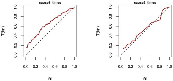
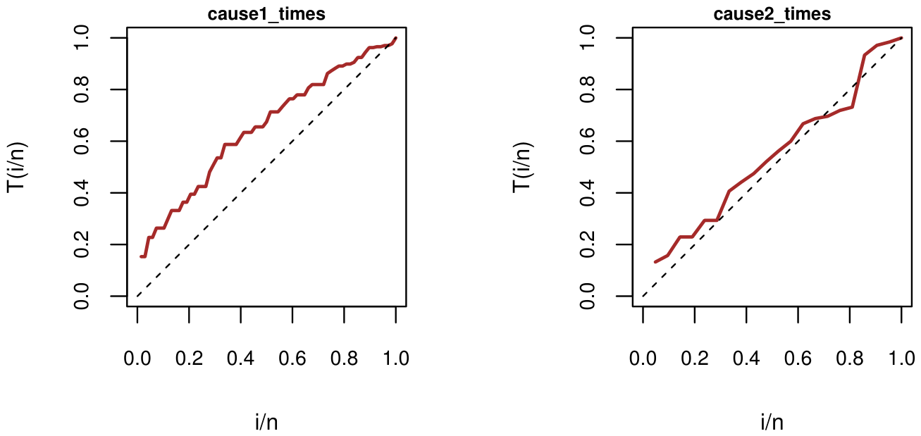
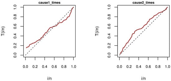
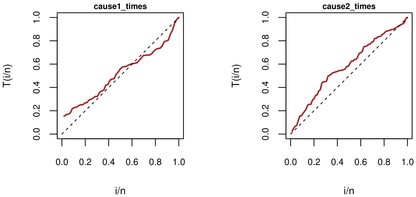
As shown in the TTT plots in Figure 5, the concavity of the TTT curve for cause 1 exhibits an increasing hazard rate (IFR), suggesting an increase probability of discharge over time as long as the patient remains in the ICU. For cause 2, the TTT curve lies along the diagonal from approximately $i/n=0$ to $i/n\approx 0.6$, referring to a constant hazard rate over an early- to middle-duration stay in the ICU, but the curve beyond $i/n\approx 0.8$ lies clearly above the diagonal, suggesting a mild augmentation in death among patients who stay in the ICU for a longer time.

Figure 5. TTT plots based on the Pneumonia dataset.

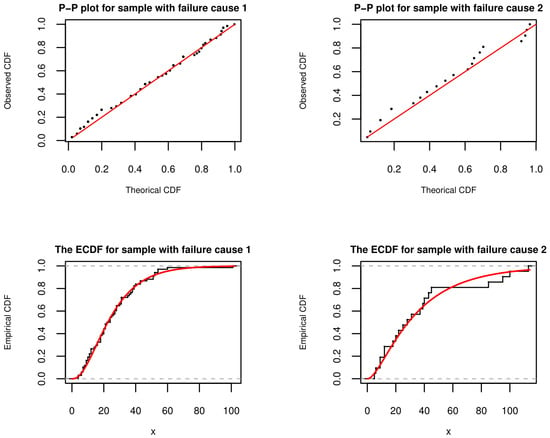
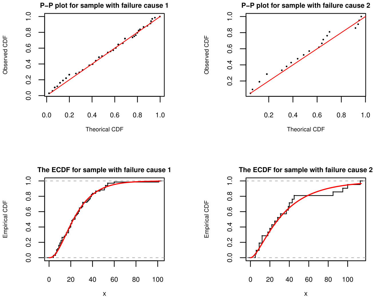
To investigate whether Stacy’s GG competing-risks model is acceptable for this dataset, the Kolmogorov–Smirnov (KS) test is conducted. For samples associated with failure cause 1, the KS test statistic is 0.06555 with a p-value of 0.932, and for samples associated with failure cause 2, the KS test statistic is 0.10748 with a p-value of 0.9685. The empirical distribution function and P-P plots are shown in Figure 6, consistent with the KS results and demonstrating the suitability of the data for the model.

Figure 6. Empirical and P-P plots based on the Pneumonia dataset.

The generated progressive Type-II censoring data with an effective sample size of $m=50$ and the data of the late censoring scheme ($R=(0^{*}49,39)$) presented as follows:

$$\begin{array}{cc}\hfill \{& (4,1),(4,1),(6,1),(6,1),(7,1),(7,1),(7,1),(8,1),(9,1),(9,1),(9,1),(10,1),\hfill \\ \hfill & (10,1),(11,1),(11,1),(12,1),(12,1),(12,1),(14,1),(15,1),(16,1),(16,1),\hfill \\ \hfill & (18,1),(18,1),(18,1),(18,1),(19,1),(20,1),(20,1),(20,1),(21,1),(21,1),\hfill \\ \hfill & (21,1),(22,1),(24,1),(24,1),(24,1),(25,1),(26,1),(27,1),(5,2),(6,2),\hfill \\ \hfill & (9,2),(9,2),(12,2),(12,2),(18,2),(20,2),(22,2),(25,2)\}.\hfill \end{array}$$

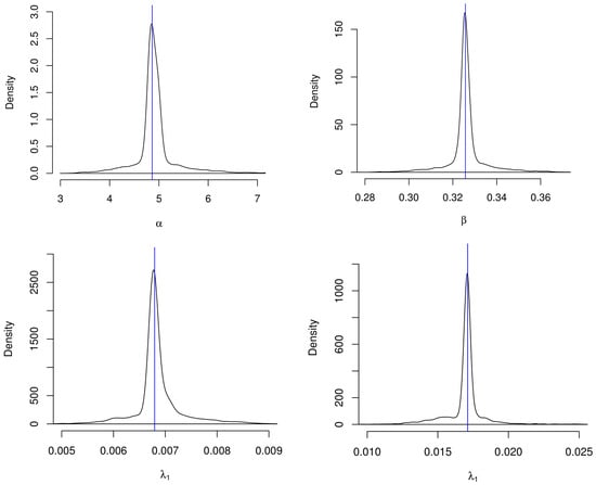
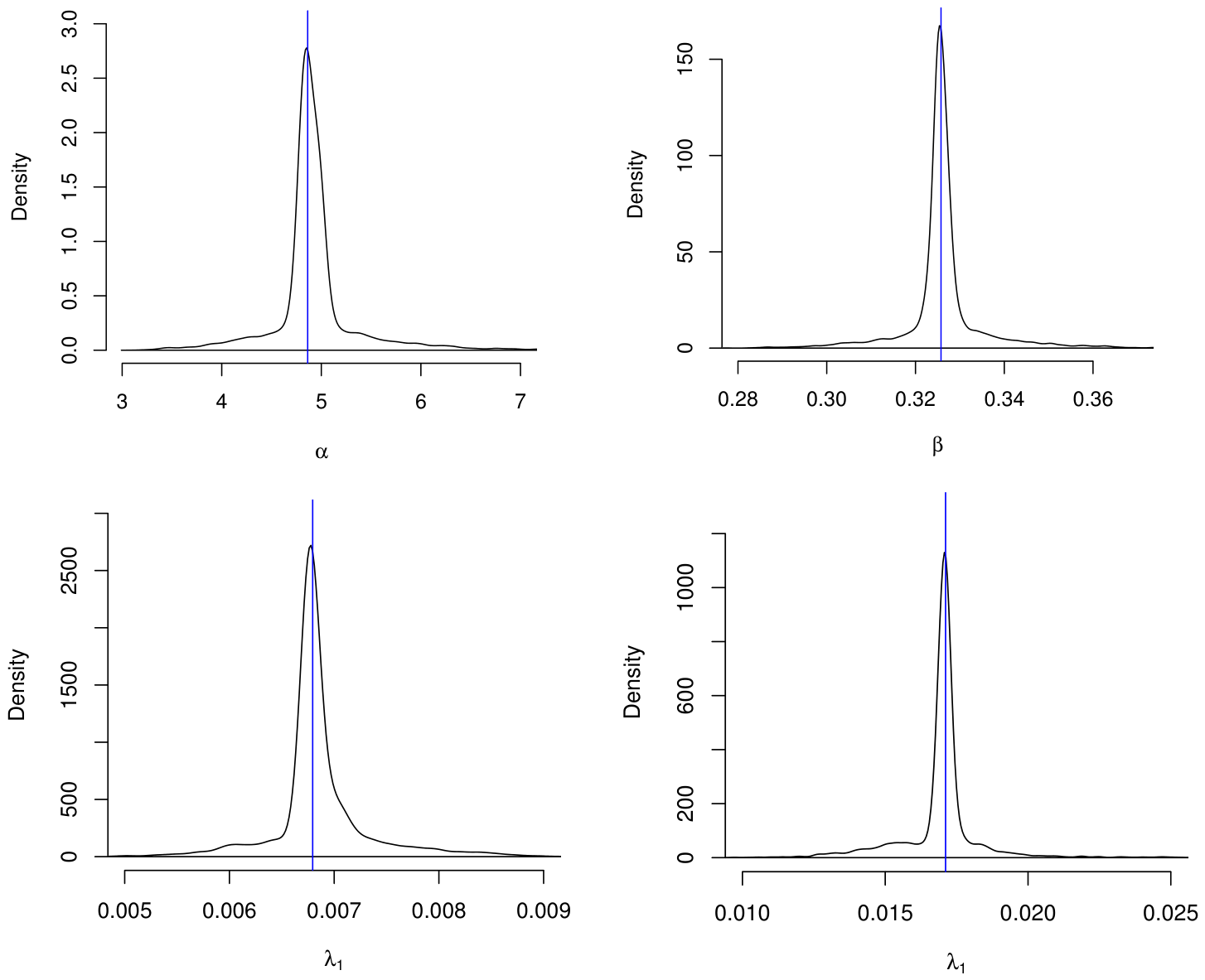
There were $m_1=40$ data points associated with failure cause 1 (discharge) and $m_2=10$ data points associated with failure cause 2 (death). Table 7 presents the parameter estimates and their corresponding RMSEs obtained using the ML and MPS methods for five different lifetime distributions: GG and its nested distributions, as well as exponential (EXP), Rayleigh (RAY), Weibull (WEI), and gamma (GAM) distributions. Figure 7 shows the density of estimates from 5000 bootstrap replications, with distinct peaks that match the real dataset estimates, indicating high accuracy and a low RMSE, particularly for the scale parameters.

Table 7. Parameter estimates and their RMSEs for pneumonia data.

Method	Model	$\widehat{\mathit{\alpha }}$	RMSE ($\widehat{\mathit{\alpha }}$)	$\widehat{\mathit{\beta }}$	RMSE ($\widehat{\mathit{\beta }}$)	$\widehat{{\mathit{\lambda }}_1}$	RMSE ($\widehat{{\mathit{\lambda }}_1}$)	$\widehat{{\mathit{\lambda }}_2}$	RMSE ($\widehat{{\mathit{\lambda }}_2}$)
ML	EXP	1	–	1	–	44.8002	7.4321	179.2025	82.9059
	RAY	2	–	2	–	32.2312	2.5469	64.4721	12.5427
	WEI	1.6906	–	1.6906	0.2340	34.0412	3.5420	77.3874	26.4049
	GAM	2.2463	0.4573	1	–	13.9104	3.5217	32.3782	14.3111
	GG	4.8630	0.0423	0.3247	0.0008	0.0068	0.0003	0.0171	0.0042
MPS	EXP	1	–	1	–	87.7166	55.1695	234.3901	144.4138
	RAY	2	–	2	–	46.7847	18.5043	76.5533	29.9887
	WEI	1.3932	–	1.3932	0.2105	61.2346	42.9379	124.0603	90.6882
	GAM	1.5740	0.7209	1	–	37.5386	23.8740	77.3114	50.3446
	GG	3.1317	1.5871	0.2564	0.0430	0.0033	0.0012	0.0079	0.0028

Figure 7. Density plots of the MLEs of $\alpha$, $\beta$, ${\lambda }_1$, and ${\lambda }_2$ based on the pneumonia dataset.

The analysis treats lifetimes associated two distinct causes and evaluates the simpler models (EXP, RAY, WEI, and GAM). Higher precision in parameter estimation corresponds to GG, which has lower RMSE values. Table 8 presents three statistical criteria to compare how well each model fits the pneumonia data: the negative of the log-likelihood function ($-\log \mathcal{L}$) to see how likely the observed data are under the estimated model; the Akaike Information Criterion (AIC) to estimate the relative quality of estimated models by balancing goodness of fit against the number of parameters of the model; and the Bayesian Information Criterion (BIC), which is similar to the AIC but provides a larger penalty for models with more parameters. Lower values for these three tools indicate a better fit. Across ML and MPS methods, the GG distribution provides the most robust fit to the pneumonia data compared to its nested models, as it consistently yields the lowest $-\log \mathcal{L}$ and AIC (e.g., AIC of 493.235 under ML). To formally justify the preference for the GG model over its simpler alternatives, Likelihood Ratio Tests (LRTs) were conducted. The tests reveal that the GG model provides a significantly improved fit compared to the EXP (${\chi }^2\left(2\right)=22.710,p<0.001$), RAY (${\chi }^2\left(2\right)=10.584,p=0.005$), WEI (${\chi }^2\left(1\right)=8.762,p=0.003$), and GAM (${\chi }^2\left(1\right)=4.930,$$p=0.026$) sub-models. This confirms that the added parametric flexibility of Stacy’s GG is statistically necessary for this dataset.

Table 8. Model comparison criteria: $-\log \mathcal{L}$, AIC, and BIC for pneumonia data.

Method	Model	$-\log \mathcal{L}$	AIC	BIC
ML	EXP	253.973	511.947	516.924
	RAY	247.910	499.819	504.796
	WEI	246.999	499.998	507.464
	GAM	245.083	496.166	503.632
	GG	242.618	493.235	503.190
MPS	EXP	19,954.918	39,913.835	39,918.813
	RAY	19,955.489	39,914.979	39,919.956
	WEI	19,953.823	39,913.646	39,921.112
	GAM	19,953.559	39,913.117	39,920.583
	GG	19,952.779	39,913.559	39,923.513

Based on pneumonia data, the three types of CIs (PBCIs, SBCIs, and ACIs) for the parameters of a model are evaluated in Table 9 using ML and MPS methods. For each parameter, the table shows the point estimate (Est), along with the lower (L) and upper (U) bounds of each CI. The $95\%$ confidence bands for $\beta$ do not contain one, so it may be unreasonable to assume that the lifetimes are GAM, and since the CIs for the two shape parameters ($\alpha$ and $\beta$), are non-intersecting, it is unlikely that they will be equal. Therefore, it may be unreasonable to consider the WEI distribution a suitable and acceptable candidate for pneumonia data. Across both ML and MPS methods, the ACI tends to be wider than the bootstrap intervals (PBCI and SBCI). For example, for ${\lambda }_2$, the ACI range under the ML method is $(0.0005,0.6404)$, whereas the PBCI is much tighter, at $(0.0133,0.0294)$. The PBCI and SBCI exhibit a large degree of consistency with one another. Since the SBCI reflects the Studentization process, which often accounts for skewness in the parameter distribution more effectively than simple percentile methods, the SBCI bounds are generally slightly shifted relative to the PBCI. Overall, the bootstrap approaches produce a more precise estimation of the uncertainty around the parameters. The MPS method produces narrower confidence bounds for several parameters, such as ${\lambda }_2$, with the lengths of the three CIs shorter than those of the ML method, suggesting that, for the pneumonia dataset, the MPS procedure offers greater stability in interval estimation.

Table 9. Lengths of PBCIs, SBCIs, and ACIs for pneumonia data.

Method	Parameter	Est	L_PBCI	U_PBCI	L_SBCI	U_SBCI	L_ACI	U_ACI
ML	$\mathit{\alpha }$	4.8630	4.0253	6.0461	3.8779	5.8258	3.3655	7.0268
	$\mathit{\beta }$	0.3247	0.3062	0.3480	0.3014	0.3520	0.2436	0.4329
	${\mathit{\lambda }}_{\mathbf{1}}$	0.0068	0.0059	0.0082	0.0053	0.0086	0.0002	0.2661
	${\mathit{\lambda }}_{\mathbf{2}}$	0.0171	0.0133	0.0294	0.0102	0.0255	0.0005	0.6404
MPS	$\mathit{\alpha }$	3.1317	2.1759	3.5222	1.6091	3.6880	1.8677	5.2513
	$\mathit{\beta }$	0.2564	0.2263	0.2690	0.2062	0.2678	0.1870	0.3515
	${\mathit{\lambda }}_{\mathbf{1}}$	0.0033	0.0027	0.0055	0.0021	0.0042	0.0001	0.1878
	${\mathit{\lambda }}_{\mathbf{2}}$	0.0079	0.0059	0.0140	0.0048	0.0121	0.0001	0.4404

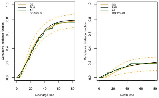
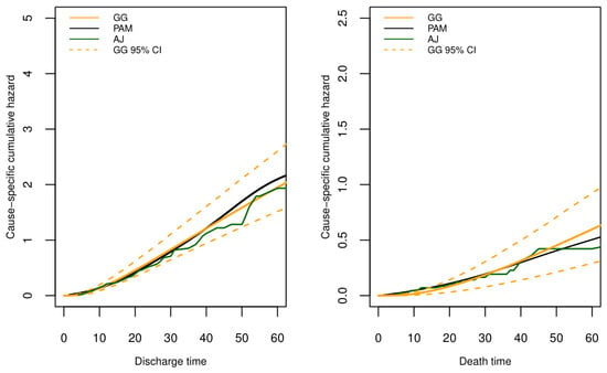
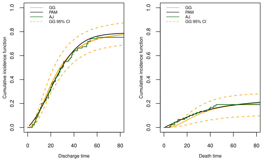
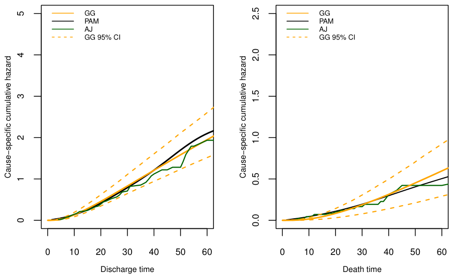
Clinically, the estimated parameters of the GG model provide actionable medical insights. The scale parameters (${\lambda }_1,{\lambda }_2$) represent the characteristic timeframes of the events, while the shape parameters ($\alpha ,\beta$) dictate the risk trajectory. For instance, the specific shape-parameter combination for discharge mathematically captures a hazard rate that rises sharply after an initial critical period, reflecting standard ICU recovery protocols. In practice, these insights enable hospital administrators to optimize ICU bed turnover and precisely anticipate high-risk mortality windows. Furthermore, to ensure clinical relevance, the GG model was benchmarked against the non-parametric Aalen–Johansen (AJ) estimator and the semi-parametric Piecewise Additive Model (PAM) estimator, both of which are standard tools in modern medical survival analysis. A study by Kopper [58] used nonparametric AJ and semi-parametric PAM approaches to construct the CIF, the cumulative hazard for each pneumonia-cause dataset, accounting for discharge and death risks. PAM models the hazard function by decomposing the lifetime into subintervals and using additive spline functions to estimate a smooth, time-varying hazard. The estimated CIFs as t tends to ∞ based on Stay’s GG competing-risks model are CIF1 = 0.7917 and CIF2 = 0.2083, referring to the fact that discharge is the dominant outcome. Figure 8 compares the CIFs obtained from the proposed Stacy’s GG competing-risks model with the nonparametric AJ estimator and the semi-parametric PAM, which were intentionally fitted to the complete lifetimes of the entire cohort. During the follow-up period, the model closely matches both competing behaviors for discharge and death outcomes. In addition, the AJ and PAM curves lie almost entirely within the $95\%$ CI obtained by Stacy’s GG competing-risks model, showing that is adequately captures the competing-risks structure of the pneumonia data. During the early follow-up period, the CIF of discharge rises rapidly before reaching a stable level near 0.80, indicating that most discharge events occur relatively early, whereas the CIF of death remains at a lower level throughout the study period and stabilizes near 0.20. Figure 8 also exhibits agreement between the model and the AJ and PAM approaches for the two risk factors (discharge and death). During most of the follow-up period, the model tracks the empirical hazard accumulation, with a slight deviation at later times due to the lack of remaining individuals at risk, especially for discharge. All three curves fall within the estimated CIs for the cumulative hazard, indicating that the proposed model, based on Stacy’s GG, adequately captures the underlying competing-risks structure of the pneumonia dataset.

Figure 8. (Top): Cumulative incidence functions (CIFs) for the pneumonia dataset. (Bottom): Cause-specific cumulative hazard functions for the pneumonia dataset.

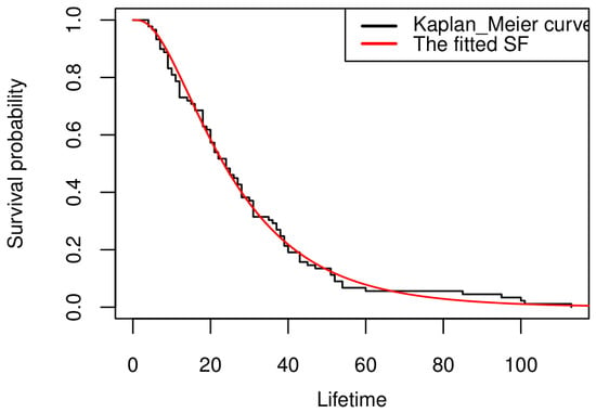
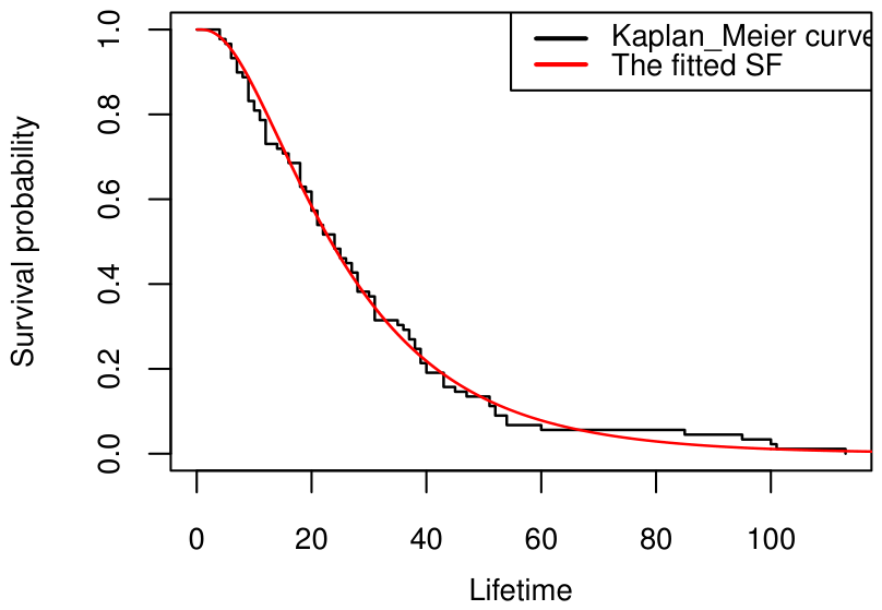
The fitted SF versus Kaplan–Meier curve of the complete sample based on late censoring in Figure 9 indicates the suitability of this censoring scheme for this dataset.

Figure 9. Comparison of the fitted SF of Stacy’s Generalized Gamma model with the empirical Kaplan–Meier curve for the complete pneumonia dataset.

6.2. Leukemia Data Analysis

The dataset includes 177 patients with acute leukemia who underwent stem cell transplantation. In this study, the incidence of relapse and mortality due to transplant-related complications is considered a competing risk. A total of 46 cases are excluded; therefore, the dataset includes 131 patients, with 56 cases of relapse (failure cause 1) and 75 cases of competing events (failure cause 2). This dataset was studied by Badwan and Pakyari [33] to fit a competing-risks model with progressively Type-II-censored data for the Dagum distribution. The dataset is available in the casebase package (v0.10.6).

As shown in the TTT plots in Figure 10, the variation of the TTT curve over time for cause 1 reveals that after transplantation, relapse may be relatively high, then settles and subsequently rises again. In contrast, the concavity of the TTT curve for cause 2 indicates that the risk of death increases in the early and intermediate periods after transplantation; then, the curve tends to become linear, indicating a more stable long-term risk.

Figure 10. TTT plots based on the Leukemia dataset.

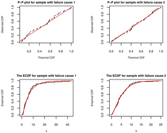
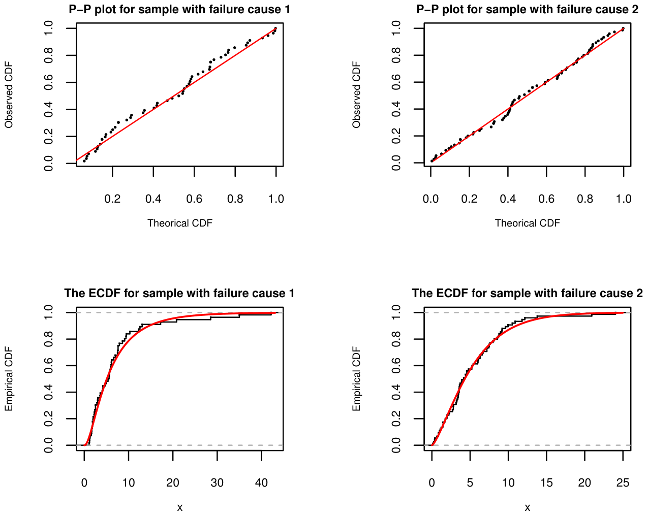
To investigate whether Stacy’s GG competing-risks model is acceptable for this dataset, the KS test is conducted. For samples associated with failure cause 1, the KS test statistic is 0.0746 with a p-value of 0.914, and for samples associated with failure cause 2, the KS test statistic is 0.06473 with a p-value of 0.9118. The empirical distribution function and P-P plots are shown in Figure 11, consistent with the KS results and demonstrating the suitability of the data for the model.

Figure 11. The Empirical and P-P plots based on the Leukemia dataset.

The generated progressive Type-II censoring data with an effective sample size of $m=40$ and an early censoring scheme ($R=(91,0^{*}39)$) are presented as follows:

$$\begin{array}{cc}\hfill \{& (1.60,1),(2.03,1),(2.30,1),(2.87,1),(3.07,1),(3.57,1),(4.73,1),(5.00,1),(5.37,1),\hfill \\ \hfill & (6.00,1),(6.13,1),(6.63,1),(7.63,1),(8.63,1),(9.50,1),(13.07,1),(35.00,1),\hfill \\ \hfill & (42.17,1),(0.13,2),(1.43,2),(1.47,2),(1.70,2),(1.97,2),(3.30,2),(3.40,2),(3.50,2),\hfill \\ \hfill & (3.57,2),(4.57,2),(4.80,2),(5.43,2),(6.60,2),(7.20,2),(7.20,2),(7.63,2),(9.17,2),\hfill \\ \hfill & (9.63,2),(9.97,2),(10.53,2),(11.80,2),(24.03,2)\}\hfill \end{array}$$

As shown in Table 10, the most precise parameter estimates across both ML and MPS approaches correspond to the GG model, as it achieves exceptionally low RMSE values compared with the nested models. This suggests that the additional parameters in the GG distribution lead to a more precise characterization of the leukemia dataset’s failure times. According to Table 11, the GG model outperforms the other models under ML and MPS methods, achieving the lowest $-\log \mathcal{L}$ and AIC, despite the BIC of GAM being considerably smaller than that of GG. Likelihood Ratio Tests (LRTs) were conducted to definitively compare the GG model against its restricted sub-models. The GG model fits the leukemia data significantly better than the EXP (${\chi }^2\left(2\right)=20.856,p<0.001$), RAY (${\chi }^2\left(2\right)=34.044,p<0.001$), WEI (${\chi }^2\left(1\right)=9.024,p=0.003$), and GAM (${\chi }^2\left(1\right)=4.484,p=0.034$) models, justifying the methodological focus on the generalized framework.

Table 10. Parameter estimates and their RMSEs for leukemia data.

Method	Model	$\widehat{\mathit{\alpha }}$	RMSE ($\widehat{\mathit{\alpha }}$)	$\widehat{\mathit{\beta }}$	RMSE ($\widehat{\mathit{\beta }}$)	$\widehat{{\mathit{\lambda }}_1}$	RMSE ($\widehat{{\mathit{\lambda }}_1}$)	$\widehat{{\mathit{\lambda }}_2}$	RMSE ($\widehat{{\mathit{\lambda }}_2}$)
ML	EXP	1	–	1	–	24.9960	6.3874	20.4514	4.6968
	RAY	2	–	2	–	17.2059	2.2538	15.4675	1.5926
	WEI	1.3789	–	1.3789	0.1639	18.2139	3.3988	15.7462	2.3941
	GAM	1.7634	0.3151	1	–	8.9125	2.7200	7.6269	1.9763
	GG	3.9942	0.0335	0.2934	0.0011	0.0017	0.0004	0.0014	0.0002
MPS	EXP	1	–	1	–	25.6687	6.9326	21.6251	5.4134
	RAY	2	–	2	–	17.9839	2.2554	16.1612	1.9087
	WEI	1.2768	–	1.2768	0.2111	19.8911	5.1696	17.2258	3.6123
	GAM	1.5413	0.3329	1	–	11.3543	6.7588	9.8011	5.1126
	GG	4.0755	0.5260	0.2462	0.0100	0.0002	3.52 $\times {10}^{-5}$	0.0001	2.64 $\times {10}^{-5}$

Table 11. Model comparison criteria ($-\log \mathcal{L}$, AIC, and BIC) for leukemia data.

Method	Model	$-\log \mathcal{L}$	AIC	BIC
ML	EXP	164.334	332.668	338.419
	RAY	170.928	345.857	351.607
	WEI	158.418	322.835	331.461
	GAM	156.148	318.296	326.922
	GG	153.906	315.812	327.313
MPS	EXP	891.263	1786.527	1792.277
	RAY	905.015	1814.029	1819.780
	WEI	888.088	1782.175	1790.801
	GAM	886.619	1779.238	1787.864
	GG	884.327	1776.655	1788.155

As shown in Table 12, the PBCI and SBCI for all parameters among ML and MPS methods are consistently narrower and more stable than the ACI. For example, the ACI under ML for ${\lambda }_1$ is $(0.00072,0.00424)$, which is a wider range compared to its PBCI $(0.00135,0.00313)$, revealing that the bootstrap-based technique provides a more reliable measure of uncertainty for the leukemia dataset. The $95\%$ confidence bands for $\alpha$ ($\beta$) via ML and MPS methods (Table 12) suggest that sub-models are unreliable for this dataset.

Table 12. Lengths of PBCIs, SBCIs, and ACIs for leukemia data.

Method	Parameter	Est	L_PBCI	U_PBCI	L_SBCI	U_SBCI	L_ACI	U_ACI
ML	$\mathit{\alpha }$	3.99418	3.22659	5.12452	3.49958	4.62055	3.22490	4.94696
	$\mathit{\beta }$	0.29344	0.27532	0.31801	0.28641	0.30419	0.26575	0.32402
	${\mathit{\lambda }}_{\mathbf{1}}$	0.00175	0.00135	0.00313	0.00162	0.00208	0.00072	0.00424
	${\mathit{\lambda }}_{\mathbf{2}}$	0.00135	0.00112	0.00230	0.00128	0.00150	0.00059	0.00311
MPS	$\mathit{\alpha }$	4.08554	2.80636	4.69000	2.81943	4.53101	3.09155	5.39912
	$\mathit{\beta }$	0.24616	0.22053	0.25751	0.22479	0.25380	0.21116	0.28697
	${\mathit{\lambda }}_{\mathbf{1}}$	0.00015	0.00012	0.00027	0.00013	0.00023	0.00001	0.00159
	${\mathit{\lambda }}_{\mathbf{2}}$	0.00013	0.00010	0.00022	0.00011	0.00019	0.00001	0.00132

Among the estimation procedures, the GG distribution provides the most robust fit among the evaluated parametric models for these specific datasets, as it consistently maximizes the accuracy of parameter estimates relative to its sub-models (EXP, RAY, WEI, and GAM) and minimizes information loss (lowest AIC). A consistent trend in estimation reliability across the pneumonia and leukemia datasets is revealed by the evaluation of the PBCI, SBCI, and ACI. The ACI frequently demonstrates the greatest width, indicating a higher degree of uncertainty. In contrast, the bootstrap-based approaches (PBCI and SBCI) provide much narrower and more stable intervals, suggesting their suitability for these specific datasets, where distributional complexity or sample size may challenge asymptotic assumptions. Despite the slight difference between the two estimation approaches, the MPS approach generally yields more compact CIs than the ML method for the scale and shape parameters, indicating its effectiveness in producing high-accuracy estimates.

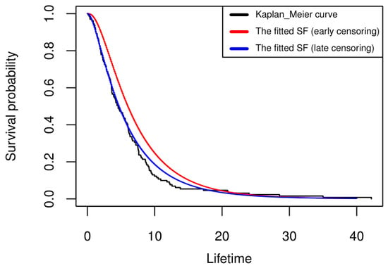
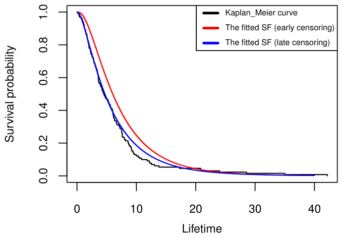
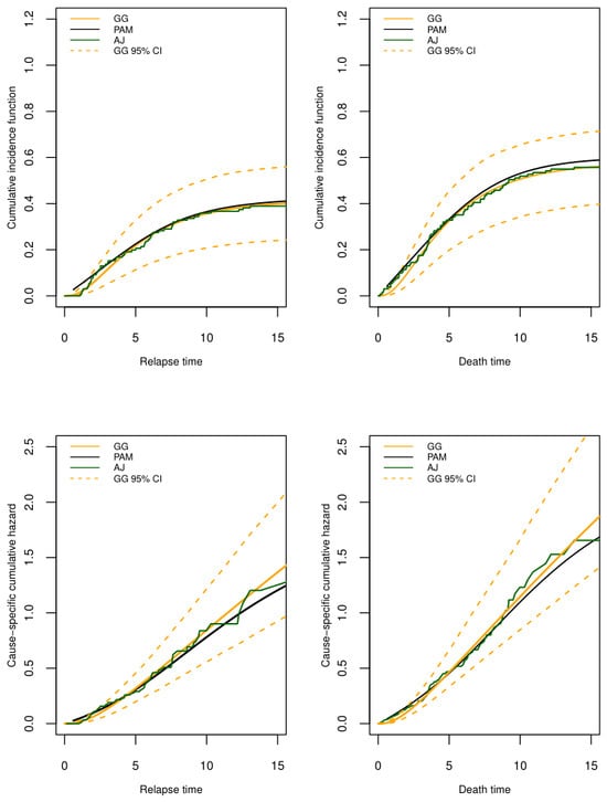
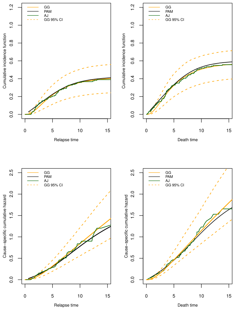
In the leukemia cohort, the clinical meaning of the parameters translates directly to post-transplant monitoring strategies. The shape parameters mathematically capture the complex biological reality of stem cell transplantation: transplant-related mortality (cause 2) peaks early due to acute complications such as graft-versus-host disease, whereas relapse (cause 1) exhibits a delayed, heavy-tailed risk profile. Practically, this parametric precision allows oncologists to tailor patient follow-up schedules, prioritizing toxicity management in the acute phase and shifting to relapse surveillance in the long term. This approach provides deeper temporal insights into patient risk than standard empirical clinical models while still closely matching the overall cumulative incidence estimates of the standard AJ and PAM approaches. To evaluate the impact of the censoring scheme on these survival estimates, the fitted SF is shown versus the Kaplan–Meier curve of the complete sample based on the leukemia dataset in Figure 12. This comparison indicates that early censoring leads to pronounced bias in survival estimates, suggesting that critical information about the hazard structure is carried by early failure times, whereas a late-censoring scheme yields a more precise survival estimate. Thus, selecting an appropriate censoring scheme is crucial, especially in clinical studies. Furthermore, Figure 13 exhibits the good matching of the model with both the AJ and PAM curves, particularly for the relapse event. The estimated CIF of death, compared with relapse, rises more rapidly over the early duration of the follow-up and stabilizes afterward, indicating that patients, with high probability experience mortality before a relapse can be observed. For both causes, the AJ and PAM curves lie within the $95\%$ CI of the model. Similarly, satisfactory consistency across the three models is observed in the cumulative hazard for death and relapse in Figure 13, although small deviations are shown at later follow-up times. Overall, Stacy’s GG competing-risks model, based on progressive censoring, successfully provides smooth and stable hazard accumulation patterns while preserving the main empirical structure reflected in the AJ and PAM estimators.

Figure 12. The fitted SF with Kaplan–Meier curve based on the leukemia dataset.

Figure 13. (Top): Cumulative incidence functions (CIFs) for the leukemia dataset. (Bottom): Cause-specific cumulative hazard functions for the leukemia dataset.

7. Concluding Discussion

In this paper, a competing-risks model based on the GG distribution under a PT-IIC scheme was considered and investigated. By integrating the GG model with a PT-IIC scheme, a methodologically rigorous framework that accounts for realistic clinical constraints is established. This allows researchers to optimize their resources while maintaining statistical validity and accuracy. Point and interval estimations for the GG model parameters were acquired using MLEs and MPSEs. In terms of point estimation, MPSEs outperform MLEs in Monte Carlo simulations in terms of consistency and efficiency, especially for the shape parameter, particularly under heavier censoring schemes and smaller effective sample sizes. On the contrary, in terms of interval estimation, ACIs achieved near-optimal coverage probabilities but were highly conservative and wider, while SBCIs provided a slight improvement in length with limited compromise in coverage, without pushing them to the extremes of the ACIs. The analysis of two medical datasets on pneumonia in the ICU and leukemia stem cell transplantation demonstrated the applicability of the considered methodology. In both scenarios, the GG distribution emerged as a highly flexible choice, outperforming its sub-models by maximizing parameter-estimation accuracy and yielding the lowest AIC. Surprisingly, the introduction of a new shape parameter led to a sharp drop in the scale parameters. The late censoring scheme for the pneumonia dataset suggests that adequate information was retained under this design, providing stable parameter estimates and an accurate fit to the observed survival function. The application of the early censoring scheme to the leukemia dataset led to significant bias in the estimated survival function, indicating that valuable information was extracted at early stages. Furthermore, consistent with the results of the Monte Carlo simulation, the MPSEs generally produce more compact confidence limits than the MLEs. Overall, the GG competing-risks model offers researchers a highly adaptable tool for complex survival analysis and life-testing trials. Much research is still underway. For instance, it is of interest to address the estimation performance under the Bayesian framework. Moreover, adopting the GG competing-risks model to accommodate more complex data structures, such as hybrid or improved progressive censoring schemes, is an important direction for future research.

References

- Crowder, M.J. Classical Competing Risks; Chapman and Hall/CRC: New York, NY, USA, 2001. [Google Scholar] [CrossRef] [Scilit]
- Monterrubio-Gómez, K.; Constantine-Cooke, N.; Vallejos, C.A. A review on competing risks methods for survival analysis. arXiv 2022, arXiv:2212.05157. [Google Scholar] [CrossRef] [Scilit]
- Monterrubio-Gómez, K.; Constantine-Cooke, N.; Vallejos, C.A. A review on statistical and machine learning competing risks methods. Biom. J. 2024, 66, 2300060. [Google Scholar] [CrossRef] [Scilit] [PubMed]
- Cox, D.R. The Analysis of Exponentially Distributed Life-Times with Two Types of Failure. J. R. Stat. Soc. Ser. B Methodol. 1959, 21, 411–421. [Google Scholar] [CrossRef] [Scilit]
- Almarashi, A.M.; Algarni, A.; Daghistani, A.M.; Abd-Elmougod, G.A.; Abdel-Khalek, S.; Raqab, M.Z. Inferences for Joint Hybrid Progressive Censored Exponential Lifetimes under Competing Risk Model. Math. Probl. Eng. 2021, 2021, 3380467. [Google Scholar] [CrossRef] [Scilit]
- Davies, K.F.; Volterman, W. Progressively Type-II censored competing risks data from the linear exponential distribution. Commun. Stat.-Theory Methods 2020, 51, 1444–1460. [Google Scholar] [CrossRef] [Scilit]
- Nassar, M.; Alotaibi, R.; Dey, S. Estimation Based on Adaptive Progressively Censored under Competing Risks Model with Engineering Applications. Math. Probl. Eng. 2022, 2022, 6731230. [Google Scholar] [CrossRef] [Scilit]
- Alghamdi, A.S.; Abd-Elmougod, G.A.; Kundu, D.; Marin, M. Statistical Inference of Jointly Type-II Lifetime Samples under Weibull Competing Risks Models. Symmetry 2022, 14, 701. [Google Scholar] [CrossRef] [Scilit]
- Ramadan, D.A.; Almetwally, E.M.; Tolba, A.H. Statistical Inference to the Parameter of the Akshaya Distribution under Competing Risks Data with Application HIV Infection to AIDS. Ann. Data Sci. 2022, 10, 1499–1525. [Google Scholar] [CrossRef] [Scilit]
- Farghal, A.W.A.; Badr, S.K.; Abu-Zinadah, H.; Abd-Elmougod, G.A. Analysis of generalized inverted exponential competing risks model in presence of partially observed failure modes. Alex. Eng. J. 2023, 78, 74–87. [Google Scholar] [CrossRef] [Scilit]
- Elshahhat, A.; Nassar, M. Inference of improved adaptive progressively censored competing risks data for Weibull lifetime models. Stat. Pap. 2023, 65, 1163–1196. [Google Scholar] [CrossRef] [Scilit]
- Dutta, S.; Ng, H.K.T.; Kayal, S. Inference for Kumaraswamy-G family of distributions under unified progressive hybrid censoring with partially observed competing risks data. Stat. Neerl. 2024, 78, 719–742. [Google Scholar] [CrossRef] [Scilit]
- Park, C.; Wang, M. Parameter Estimation of Birnbaum-Saunders Distribution under Competing Risks Using the Quantile Variant of the Expectation-Maximization Algorithm. Mathematics 2024, 12, 1757. [Google Scholar] [CrossRef] [Scilit]
- Alotaibi, R.; Rezk, H.; Park, C. Parameter estimation of inverse Weibull distribution under competing risks based on the expectation–maximization algorithm. Qual. Reliab. Eng. Int. 2024, 40, 3795–3808. [Google Scholar] [CrossRef] [Scilit]
- Alhidairah, S.; Alam, F.M.A.; Nassar, M. A new competing risks model with applications to blood cancer data. J. Radiat. Res. Appl. Sci. 2024, 17, 101001. [Google Scholar] [CrossRef] [Scilit]
- Ahmed, S.M.; Abdalla, M.; Farghal, A.W.A. Statistical inference for competing risks model with Type-II generalized hybrid censored of inverse Lomax distribution with applications. Alex. Eng. J. 2025, 118, 132–146. [Google Scholar] [CrossRef] [Scilit]
- Alotaibi, R.; Nassar, M.; Khan, Z.A.; Alajlan, W.A.; Elshahhat, A. Analysis and data modelling of electrical appliances and radiation dose from an adaptive progressive censored XGamma competing risk model. J. Radiat. Res. Appl. Sci. 2025, 18, 101188. [Google Scholar] [CrossRef] [Scilit]
- Alam, F.M.A.; Daghistani, A.M.; Almufarrej, D. On Stacy’s Generalized Gamma Competing Risks Model: Estimation Procedure with Applications to Blood Cancer Data. Mathematics 2025, 13, 3818. [Google Scholar] [CrossRef] [Scilit]
- Stacy, E.W. A Generalization of the Gamma Distribution. Ann. Math. Stat. 1962, 33, 1187–1192. [Google Scholar] [CrossRef] [Scilit]
- Balakrishnan, N.; Aggarwala, R. Progressive Censoring; Birkhäuser: Boston, MA, USA, 2000. [Google Scholar] [CrossRef] [Scilit]
- Balakrishnan, N.; Kundu, D. Hybrid censoring: Models, inferential results and applications. Comput. Stat. Data Anal. 2013, 57, 166–209. [Google Scholar] [CrossRef] [Scilit]
- Balakrishnan, N.; Cramer, E. The Art of Progressive Censoring: Applications to Reliability and Quality; Springer: New York, NY, USA, 2014. [Google Scholar] [CrossRef] [Scilit]
- Kundu, D.; Kannan, N.; Balakrishnan, N. Analysis of progressively censored competing risks data. In Handbook of Statistics; Elsevier Science B.V.: Amsterdam, The Netherlands, 2003; Volume 23, pp. 331–348. [Google Scholar]
- Sarhan, A.M. Analysis of incomplete, censored data in competing risks models with generalized exponential distributions. IEEE Trans. Reliab. 2007, 56, 132–138. [Google Scholar] [CrossRef] [Scilit]
- Kundu, D.; Joarder, A. Analysis of type-II progressively hybrid censored competing risks data. J. Mod. Appl. Stat. Methods 2006, 5, 152–170. [Google Scholar] [CrossRef] [Scilit]
- Pareek, B.; Kundu, D.; Kumar, S. On progressively censored competing risks data for Weibull distributions. Comput. Stat. Data Anal. 2009, 53, 4083–4094. [Google Scholar] [CrossRef] [Scilit]
- Koley, A.; Kundu, D. On generalized progressive hybrid censoring in presence of competing risks. Metrika 2017, 80, 401–426. [Google Scholar] [CrossRef] [Scilit]
- Hemmati, F.; Khorram, E. On adaptive progressively Type-II censored competing risks data. Commun. Stat.-Simul. Comput. 2017, 46, 4671–4693. [Google Scholar] [CrossRef] [Scilit]
- Ren, J.; Gui, W. Statistical analysis of adaptive type-II progressively censored competing risks for Weibull models. Appl. Math. Model. 2021, 98, 323–342. [Google Scholar] [CrossRef] [Scilit]
- Dutta, S.; Kayal, S. Inference of a competing risks model with partially observed failure causes under improved adaptive type-II progressive censoring. Proc. Inst. Mech. Eng. O J. Risk Reliab. 2023, 237, 765–780. [Google Scholar] [CrossRef] [Scilit]
- Hassan, A.S.; Mousa, R.M.; Abu-Moussa, M.H. Analysis of Progressive Type-II Competing Risks Data, with Applications. Lobachevskii J. Math. 2022, 43, 2479–2492. [Google Scholar] [CrossRef] [Scilit]
- Tian, Y.; Liang, Y.; Gui, W. Inference and optimal censoring scheme for a competing-risks model with type-II progressive censoring. Math. Popul. Stud. 2024, 31, 1–39. [Google Scholar] [CrossRef] [Scilit]
- Badwan, R.; Pakyari, R. Analyzing Competing Risks with Progressively Type-II Censored Data in Dagum Distributions. Axioms 2025, 14, 508. [Google Scholar] [CrossRef] [Scilit]
- Alhidairah, S.; Alam, F.M.A.; Nassar, M. Failure Cause Analysis Under Progressive Type-II Censoring Using Generalized Linear Exponential Competing Risks Model with Medical and Industrial Applications. Axioms 2025, 14, 595. [Google Scholar] [CrossRef] [Scilit]
- Burnham, K.P.; Anderson, D.R. Model Selection and Multimodel Inference, 2nd ed.; Springer: New York, NY, USA, 2004. [Google Scholar] [CrossRef] [Scilit]
- Chakrabarti, A.; Ghosh, J.K. AIC, BIC and Recent Advances in Model Selection. In Philosophy of Statistics; Elsevier: Amsterdam, The Netherlands, 2011; pp. 583–605. [Google Scholar] [CrossRef] [Scilit]
- Murage, P.; Mung’atu, J.; Odero, E. Optimal Threshold Determination for the Maximum Product of Spacing Methodology with Ties for Extreme Events. Open J. Model. Simul. 2019, 7, 149–168. [Google Scholar] [CrossRef]
- Cheng, R.C.H.; Amin, N.A.K. Maximum Product-of-Spacings Estimation with Applications to the Lognormal Distribution; Technical Report 1; University of Wales IST, Department of Mathematics: Cardiff, UK, 1979. [Google Scholar]
- Cheng, R.C.H.; Amin, N.A.K. Estimating Parameters in Continuous Univariate Distributions with a Shifted Origin. J. R. Stat. Soc. Ser. B Stat. Methodol. 1983, 45, 394–403. [Google Scholar] [CrossRef] [Scilit]
- Ranneby, B. The Maximum Spacing Method. An Estimation Method Related to the Maximum Likelihood Method. Scand. J. Stat. 1984, 11, 93–112. [Google Scholar]
- Ghosh, K.; Jammalamadaka, S. A general estimation method using spacings. J. Stat. Plan. Inference 2001, 93, 71–82. [Google Scholar] [CrossRef] [Scilit]
- Efron, B. The Jackknife, the Bootstrap and Other Resampling Plans; SIAM: Philadelphia, PA, USA, 1982. [Google Scholar]
- Hall, P. Theoretical comparison of bootstrap confidence intervals. Ann. Stat. 1988, 16, 927–953. [Google Scholar] [CrossRef] [Scilit]
- Gupta, R.D.; Kundu, D. Generalized exponential distribution: Different method of estimations. J. Stat. Comput. Simul. 2001, 69, 315–337. [Google Scholar] [CrossRef] [Scilit]
- Alkasasbeh, M.R.; Raqab, M.Z. Estimation of the generalized logistic distribution parameters: Comparative study. Stat. Methodol. 2009, 6, 262–279. [Google Scholar] [CrossRef] [Scilit]
- Mazucheli, J.; Louzada, F.; Ghitany, M. Comparison of estimation methods for the parameters of the weighted Lindley distribution. Appl. Math. Comput. 2013, 220, 463–471. [Google Scholar] [CrossRef] [Scilit]
- do Espirito Santo, A.; Mazucheli, J. Comparison of estimation methods for the Marshall–Olkin extended Lindley distribution. J. Stat. Comput. Simul. 2014, 85, 3437–3450. [Google Scholar] [CrossRef] [Scilit]
- Balakrishnan, N.; Alam, F.M.A. Maximum likelihood estimation of the parameters of Student’s t Birnbaum-Saunders distribution: A comparative study. Commun.-Stat.-Simul. Comput. 2019, 51, 793–822. [Google Scholar]
- Nassar, M.; Okasha, H.; Albassam, M. E-Bayesian estimation and associated properties of simple step–stress model for exponential distribution based on type-II censoring. Qual. Reliab. Eng. Int. 2020, 37, 997–1016. [Google Scholar] [CrossRef] [Scilit]
- Alam, F.M.A.; Nassar, M. On Modeling Concrete Compressive Strength Data Using Laplace Birnbaum-Saunders Distribution Assuming Contaminated Information. Crystals 2021, 11, 830. [Google Scholar] [CrossRef] [Scilit]
- Alam, F.M.A.; Almalki, A.M. The hazard rate function of the logistic Birnbaum-Saunders distribution: Behavior, associated inference, and application. J. King Saud Univ.-Sci. 2021, 33, 101580. [Google Scholar] [CrossRef] [Scilit]
- Moloy, D.J.; Ali, M.A.; Alam, F.M.A. Modeling Climate data using the Quartic Transmuted Weibull Distribution and Different Estimation Methods. Pak. J. Stat. Oper. Res. 2023, 19, 649–669. [Google Scholar] [CrossRef] [Scilit]
- Posit Team. RStudio: Integrated Development Environment for R; Posit Software, PBC: Boston, MA, USA, 2025. [Google Scholar]
- R Core Team. R: A Language and Environment for Statistical Computing; R Foundation for Statistical Computing: Vienna, Austria, 2025. [Google Scholar]
- Johnson, S.G. The NLopt Nonlinear-Optimization Package. 2008. Available online: https://nlopt.readthedocs.io/en/latest/Citing_NLopt/ (accessed on 30 June 2026).
- Powell, M. The BOBYQA Algorithm for Bound Constrained Optimization Without Derivatives; Technical Report; Department of Applied Mathematics and Theoretical Physics, Centre for Mathematical Sciences: Cambridge, UK, 2009. [Google Scholar]
- Wolkewitz, M.; Vonberg, R.P.; Grundmann, H.; Beyersmann, J.; Gastmeier, P.; Bärwolff, S.; Geffers, C.; Behnke, M.; Rüden, H.; Schumacher, M. Risk factors for the development of nosocomial pneumonia and mortality on intensive care units: Application of competing risks models. Crit. Care 2008, 12, R44. [Google Scholar] [CrossRef] [Scilit] [PubMed]
- Kopper, P. Flexible Estimation of Complex Effects in the Context of Competing Risks Survival Analysis: Exposure-Lag-Response Association of Artificial Nutrition and Patients’ Length of Stay in Intensive Care Units. Master’s Thesis, Ludwig Maximilian University Munich, Munich, Germany, 2020. [Google Scholar]
Disclaimer/Publisher’s Note: The statements, opinions and data contained in all publications are solely those of the individual author(s) and contributor(s) and not of MDPI and/or the editor(s). MDPI and/or the editor(s) disclaim responsibility for any injury to people or property resulting from any ideas, methods, instructions or products referred to in the content. |
© 2026 by the authors. Licensee MDPI, Basel, Switzerland. This article is an open access article distributed under the terms and conditions of the Creative Commons Attribution (CC BY) license.