


Abstract
To address insufficient representativeness and the potential risk of the underestimation of the long-term atmospheric diffusion assessment of nuclear facility gaseous effluents, a CFD numerical simulation framework based on annual joint-frequency weighting of 16 wind directions, 6 wind speed classes and 6 atmospheric stability classes is proposed and applied to a representative multi-source nuclear facility. The regulation law of near-surface flow field of the building complex and the diffusion characteristics of uranium aerosol is analyzed. The results indicate: Complex building matrix facilitates the formation of recirculating wake regions, which may serve as potential zones for aerosol accumulation. The uranium aerosol concentration weighted by joint frequency presents a distribution characteristic of central agglomeration and asymmetric gradient attenuation. Compared with the single most-frequent meteorological scenario, the joint-frequency-weighted field shows a higher expected peak and a 237 m shift in peak position. This shows that the joint-frequency weighting framework can reduce directional bias and underestimation of hotspot extent relative to a most-frequent meteorological condition. The method may provide quantitative support for refined radiation protection management and the environmental monitoring layout of nuclear facilities.
1. Introduction
The characteristics of the long-term distribution of nuclear industrial pollution are the key basis of occupational health assessments and environmental management decision-making [1,2,3,4,5,6]. Accurate characterization of the coupling between meteorological probabilistic features and the diffusion of pollutants is critical to realize annual pollution assessments and hotspot analyses at a nuclear site.
Atmospheric diffusion of nuclear pollutants is highly sensitive to meteorological parameters, including wind direction, wind speed and atmospheric stability classes. Pollution diffusion extends in different directions according to wind direction. Its vertical dispersion capacity and diffusion rate are significantly affected by atmospheric stability and complex aerosol dynamics in turbulent boundary layers [4,7,8]. This effect is particularly pronounced at multi-source nuclear sites, where overlapping plumes and complex site conditions amplify meteorological effects on pollution.
Current studies on industrial pollution diffusion show some technical limitations. Many CFD studies are conducted under selected meteorological scenarios to clarify near-field flow and concentration mechanisms [9,10,11,12,13,14,15,16,17,18,19]. This approach only captures the pollution diffusion under specific meteorological conditions, but ignores the variability of meteorological factors throughout the year, and fails to address the long-term accumulation effect of pollution. This leads to a deviation between the simulation result/assessment and the actual pollution accumulation, and also affects the data support for pollution hotspot identification and health risk assessment at nuclear sites.
In terms of recent research progress, recent studies have improved the understanding of physical mechanisms of pollution diffusion, such as turbulence parameterization, analysis of source terms [9,11,12,13,14], or classic building wake validation [15,16,20]. Nevertheless, a technical gap remains on annual-scale probabilistic pollution modeling. Existing studies mostly focus on a short-term episode (like a monsoon period or heavy pollution period), or neglect the differences in annual joint frequencies [5,6]. The gap directly results in the key practical problems including annual pollution hotspot identification or long-term occupational exposure assessment. For example, an extreme meteorological condition may lead to a pollution diffusion up to 3000 m with a possibility around 1%. Its contribution to annual accumulation is far lower than a condition where pollution diffuses 1000 m but with a possibility around 30%. This non-linear frequency-effect represents a key limitation of the traditional single-scenario approach [5,6].
Existing atmospheric dispersion assessment approaches can be broadly divided into regulatory probabilistic methods and high-resolution CFD-based methods. Regulatory long-term assessments usually rely on simplified dispersion formulations and have limited ability to resolve building-induced recirculation, wake effects, and multi-source plume interactions in the near field; CFD-based studies can explicitly represent terrain, building geometry, and local flow structures around nuclear facilities, but they are often performed for several selected meteorological scenarios because of the computational cost of multi-scenario simulations. A methodological gap exists between long-term probabilistic assessment and building-resolved near-field CFD analysis.
The novelty of this study is to help in bridging this gap by combining building-resolved CFD simulations with annual meteorological joint-frequency weighting. Specifically, a multi-scenario CFD workflow is established for 16 wind directions, 6 wind speed classes, and 6 atmospheric stability classes. The resulting concentrations are superposed with annual occurrence frequencies. This framework does not replace regulatory dose assessment or site-specific monitoring validation. Instead, it provides a screening-level method for reconstructing an annual expected near-field concentration map and identifying potential hotspot regions at multi-source nuclear production sites.
2. Materials and Methods
This study establishes a CFD numerical simulation (Openfoam9) based on joint-frequency-weighted superposition to investigate annual pollution distribution characteristic and hotspot distribution in a typical multi-source nuclear industrial site. The workflow includes geometry modeling, CFD meshing, numerical settings, parametric sweep and joint-frequency weighting.
A predefined multi-source nuclear industrial production site is constructed in this study, including about a hundred buildings with heights ranging from 4 m to 28 m and eight release stacks. The parameters of the stacks are listed in Table 1. These parameters are set with reference to some publicly available practical factories.
Table 1.
Stack parameter settings.
Uranium particles are modeled as a continuous dilute species with Eulerian concentration field approach. In this study, all gaseous effluents from nuclear facilities are assumed to have passed through high-efficiency particulate air (HEPA) filtration and cooling systems before discharge. Consequently, the pollutant is sub-micron particles with their emission temperature reduced to the ambient atmospheric temperature. Hence, the release is treated as cold-source release and thermal buoyancy effect is neglected as a modeling assumption. The joint frequencies of meteorological factors are preset based on long-term local meteorological monitoring data. These frequencies provide a weighting basis for the subsequent superposition of simulation results under different conditions. The joint frequency used is provided in the Supplementary Materials.
2.1. Geometry Modeling and Rotation Configuration
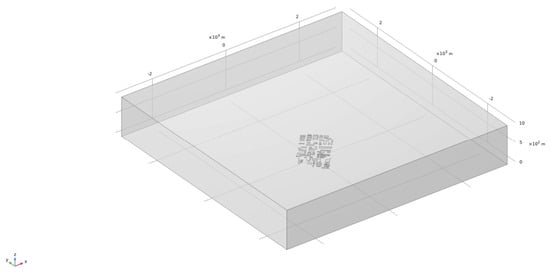
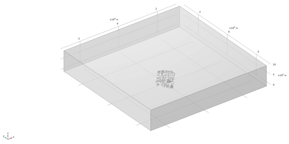
The computational domain is designed as a 2.5 km × 2.5 km × 1 km rectangular space, centered on the nuclear site center. A representative schema of the computational domain is shown in Figure 1. This size was selected to cover the facility-scale near-field region, the building cluster, the stack-release area, and the main plume-development region considered in this screening study. The horizontal and vertical extents keep the external boundaries sufficiently separated from the main building group, thereby reducing artificial boundary constraints while maintaining feasible computational cost for the multi-scenario simulations.
Figure 1.
Schematic view of the CFD computational domain used for the representative multi-source nuclear production site. The domain is a rectangular space of 2.5 km × 2.5 km × 1.0 km, centered at the site center. The horizontal coordinates x and y are given in meters, and the vertical coordinate z represents height above ground level in meters. The figure illustrates the computational extent and relative arrangement of the site geometry; for different wind directions, the domain is rotated so that the inlet boundary is perpendicular to the prescribed incoming wind direction.
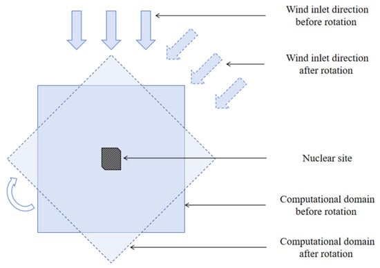
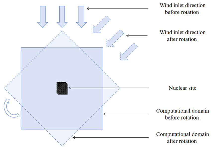
A rotation configuration (a schematic diagram sees Figure 2) is adopted to benefits the subsequent superposition of pollution maps after simulation. The edges of computing domains are rotated to be always perpendicular to the inlet wind direction (N, NNE, NE, ENE, E, ESE, SE, SSE, S, SSW, SW, WSW, W, WNW, NW, NNW) while maintaining the orientation of the nuclear site. In total, 16 distinct computing models are formed as results, each refers to a distinct inlet wind direction.
Figure 2.
Schematic diagram of the rotation of computational domain.
2.2. CFD Meshing
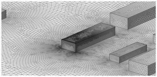
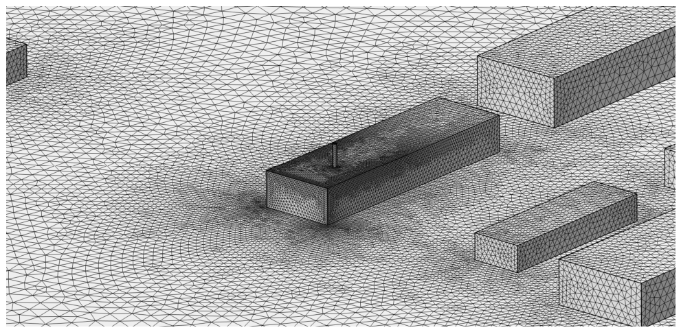
Tetrahedral grids are majorly generated to adapt to the complex geometric buildings and stacks. To improve the accuracy of flow and pollutant dispersion in key areas, 5 layers of refined mesh are implemented at the corners of buildings and chimneys, with a stretching factor of 1.2 and a thickness adjustment factor of 2.5. A local zooming of refined mesh near buildings is shown in Figure 3.
Figure 3.
Local zooming of mesh near buildings.
The general parameter settings of mesh are as follows: The minimum mesh size is 0.5 m and the maximum mesh size is 2 m, determined according to the geometric scale of the buildings. The maximum growth rate of the mesh is set as 1.2, and the curvature factor is set as 0.2 to ensure the accuracy of grid on surface of the stacks.
A grid independence verification is carried out by comparing the maximum of uranium concentration on the ground of nuclear site with meshes of different densities (1.5 million, 2 million, 2.6 million, 3.1 million and 3.5 million elements). The results show that the variation in concentration is less than 1% when the number of mesh elements is higher than 2.6 million, indicating sufficient mesh resolution for the simulation.
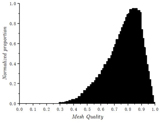
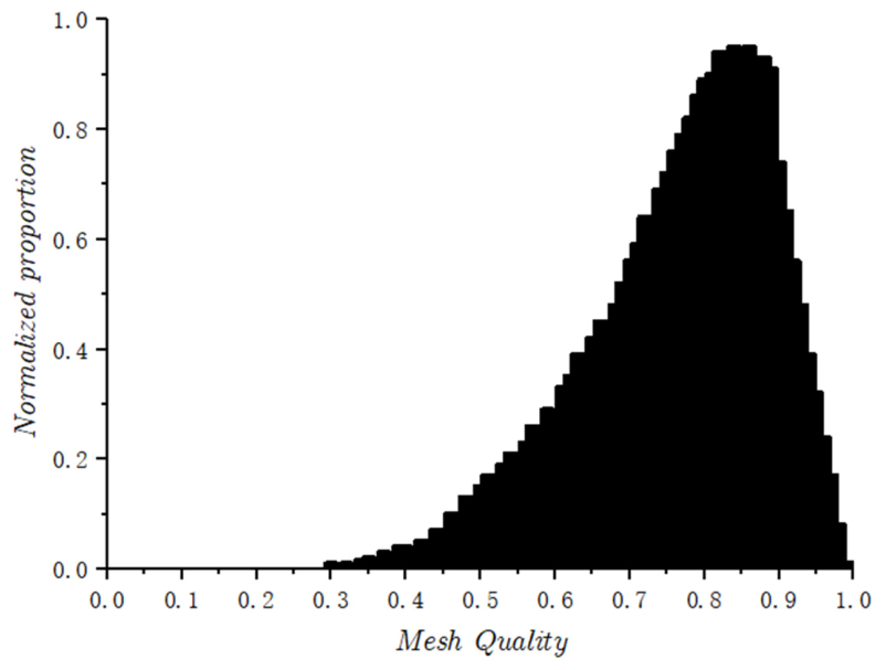
The final mesh contains 2,630,149 elements and 583,156 vertices. The histogram of mesh quality is shown in Figure 4. An average meshing element quality of 0.7639 is reached.
Figure 4.
Histogram of meshing element quality.
2.3. Numerical Settings
To simulate the site-scale pollutant distribution, the realizable k-ε model is employed to establish a fluid-thermal-solid multiphysics coupling simulation model. The control equation, boundary conditions and computing parameters used are as follows:
2.3.1. Fluid Flow
The governing equations for fluid flow obey mass, momentum, and energy conservation laws, as:
- 1.
- Mass conservationwhere ρ represents fluid density, and represents the velocity vector.
- 2.
- Momentum Conservation Equationwhere represents dynamic viscosity; represents pressure and represents volumetric force.
- 3.
- Energy Conservation Equationwhere represents temperature; represents thermal conductivity; represents viscous dissipation; and represents volumetric heat source.
2.3.2. Turbulence Model
The realizable k-ε model is able to achieve high accuracy for attached flows, jets, and channel flows, which are dominant in nuclear facilities and building-influenced near-field regions [17,18,19,21]. It is also a suitable model to deal with wall-dominated boundary layers and complex terrain flows around structures, and has proven to be an appropriate choice in many site diffusion research studies. The transport equations of the realizable k-ε model are as follows:
- 1.
- Turbulent Kinetic Energywhere represents fluid density, represents turbulent kinetic energy, represents time, represents velocity component in the -direction, represents coordinate in the -direction, represents molecular dynamic viscosity, represents turbulent viscosity, represents turbulent Prandtl number for , represents production of turbulent kinetic energy, and represents turbulent dissipation rate.
- 2.
- Dissipation Ratewhere represents turbulent Prandtl number for , represents magnitude of the mean strain rate, represent model constants, and represents turbulent kinetic energy.
- 3.
- Turbulent Energy Production Termwhere represents production of turbulent kinetic energy, represents turbulent viscosity, and represents magnitude of the mean strain rate.
The reference pressure and temperature in the simulations are set as 1 atm and 293.15 K, respectively.
2.3.3. Species Transport
The description of the pollution dispersion in this simulation is realized by the Transport of Diluted Species (TDS) equation, which solves the convection-diffusion equation. The law quantifies diffusive flux proportional to concentration gradients integrated with the mass continuity equation: . Integrating advection with Fickian diffusion yields the convection-diffusion equation as follows.
where C is the concentration, u represents the velocity vector, R represents the volumetric source term, and D represents the effective diffusion coefficient.
2.3.4. Boundary Conditions
The velocity definition of the inlet surfaces of computing area follows the power law of wind shear.
where is the mean wind speed at 10 m height and is the wind profile exponent.
Vertical temperature gradient incorporates atmospheric stability effects. The values of under different stability classes are shown in Table 2.
Table 2.
Wind exponent and lapse rate in simulation.
The outlet boundary is set as a static pressure boundary with p = patm. The ground boundary is set as a no-slip condition to simulate the friction effect of ground surface. The other boundaries are set as open boundaries to ensure the airflow can enter or exit the computational domain without limitation.
The outlets of stacks are set as uniform normal velocity boundaries, with the velocity direction perpendicular to the outlet surface. The uranium pollutant release rates are calculated according to different emission intensities and velocities. The turbulent Schmidt number is set to 0.7 for species transport, following commonly used values in CFD dispersion simulations [23]. This parameter was adopted to maintain consistency across all meteorological scenarios in the screening-level analysis.
2.4. Parametric Sweep and Joint-Frequency Weighting Algorithm
A probabilistic method with joint frequency is established to realize annual nuclear pollution distribution and hotspot assessments. The workflow of this method is as follows:
- Configuration of CFD simulations:
Based on the numerical model of nuclear site, processing body meshing, numerical model establishment and boundary condition configuration are employed to achieve CFD simulations.
- 2.
- Parametric sweep of joint frequency:
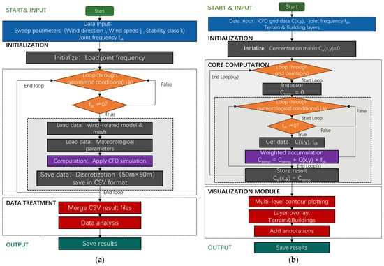
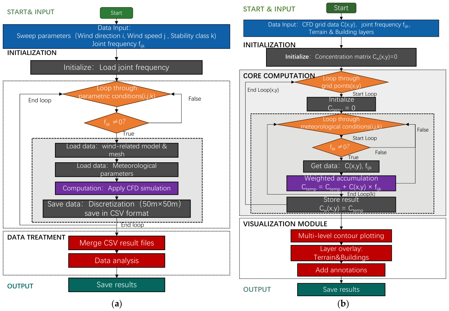
A parametric sweep algorithm is developed to perform automatic CFD simulations for multiple combinations of parameters, including wind direction, wind speed and atmospheric stability. The flow chart of this algorithm is shown in Figure 5a.
Figure 5.
Flow chart of algorithms. (a) Parametric sweep; (b) result visualization.
The algorithm starts with an input of meteorological parameters, including wind speed u, wind direction θ, atmospheric stability and corresponding joint-frequency weight . By loading the joint-frequency data, an iterative loop is initiated to sweep all parametric meteorological combinations. The combinations with = 0 are automatically passed to minimize total computing time. For each validated combination, precomputed model and mesh are loaded with CFD simulation boundary conditions. Then the CFD simulation is executed to solve pollution distribution in the specific meteorological combination. The computing results are discretized into a 50 m × 50 m nodal grid and saved as a comma-separated CSV file. After finishing computing all combinations, the distributed CSV result files are consolidated into a dataset, and output for subsequent visualization and hotspot identification.
The following boundary condition parameters are encompassed:
- Wind direction: 16 discrete bearings (N, NNE, NE, ENE, E, ESE, SE, SSE, S, SSW, SW, WSW, W, WNW, NW, NNW).
- Wind speed: Six velocities, following the averages or representative velocities of 6 velocity groups of joint frequency, as 0.5 m/s,1.5 m/s, 2.5 m/s, 4 m/s, 5.5 m/s and 6.5 m/s.
- Atmospheric stability: Six classes (A–F per Pasquill–Gifford).
This yielded 576 computational cases (16 × 6 × 6) in maximum. In practice, the number of computational cases will be substantially reduced by skipping those with joint-frequency weight at 0.
- 3.
- Visualization Process of Results
For each combination of wind direction , wind speed class , and stability class , a steady-state CFD simulation provides the ground-level activity concentration field (Bq·m−3). The annual joint frequency is obtained from long-term site meteorological observations (Supplementary Table S1). Before superposition, each scenario contribution is stored as . The annual expected concentration field is
where is interpreted as a probability-weighted long-term representative concentration map for hotspot screening.
The flow chart of visualization algorithm is shown in Figure 5b.
2.5. Model Verification with Wind-Tunnel Result
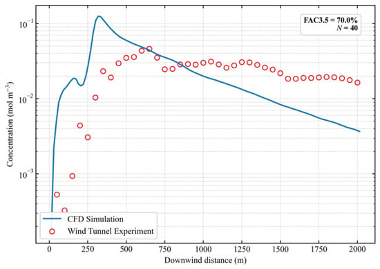
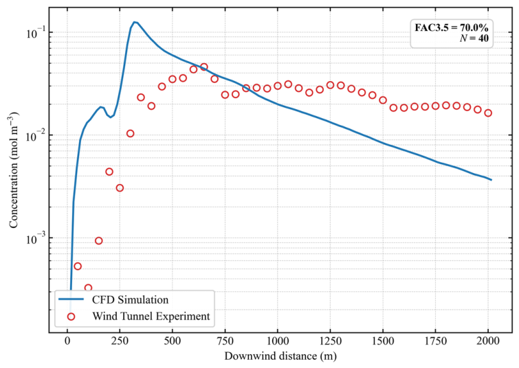
For model validation, a quantitative comparison was performed against our wind-tunnel experimental data for the nuclear site under (Figure 6). The wind-tunnel experiment simulated the atmospheric dispersion under the most-frequent meteorological scenario (i.e., ESE wind direction, D-class stability, and a representative wind speed of 4.0 m/s). The wind-tunnel experiment and validation CFD simulation were conducted under a unit source strength (e.g., 1 mol·s−1). The simulated concentration profile is in good agreement with the experimental measurements, with 70.0% of the paired downwind concentration points satisfying the factor–of–3.5 criterion (FAC3.5 = 70.0%), which is used here as a screening-level dispersion-model performance indicator [20]. This comparison provides preliminary support for the selected computing parameter settings in dispersion characteristics.
Figure 6.
Quantitative downwind validation of the CFD dispersion model against wind-tunnel experimental measurements. The profile represents the ground-level concentration along the down-wind centerline passing through the peak ground-level concentration point. The statistical evaluation index FAC3.5 is 70.0% for the N = 40 paired downwind locations.
3. Results
3.1. Local Flow Field Distribution Characteristics
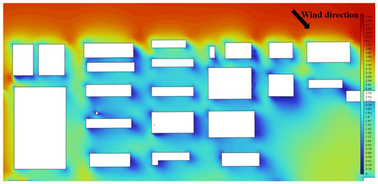
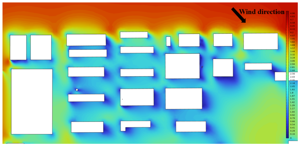
Figure 7 represents the distribution of wind field in the site under north wind inlet direction. The wind speed shows a gradient attenuation along the flow path, as the incoming flow successively passes through multiple rows of buildings. Several low-speed wind corridors form inside the building cluster. These wind distribution characteristics are the key controlling factor which affects the atmospheric turbulent transport at the block scale and the final pollutant dispersion in the study area.
Figure 7.
Characteristics and sampling points in local flow field.
3.2. Near Surface Flow Field on Windward and Leeward Sides of Building Complex
3.2.1. Velocity Distribution on Windward and Leeward Sides of the Buildings Under Different Inlet Wind Speeds
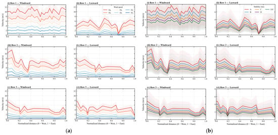
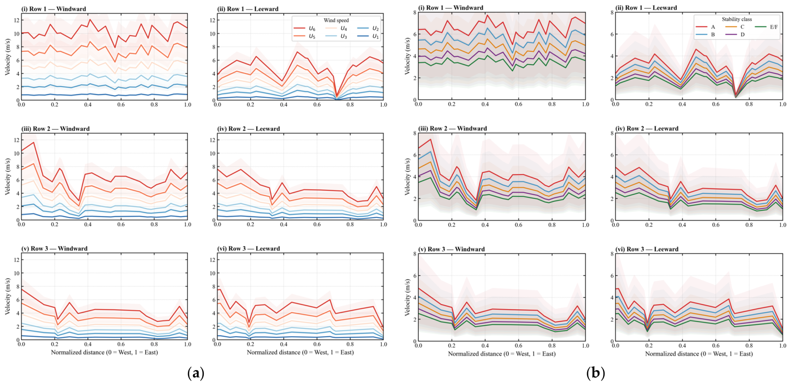
Figure 8a presents a near surface wind velocity distribution along the normalized distance on the windward (solid line) and leeward (dashed line) sides of three consecutive building rows (Row 1-Row 3) under five sets of increasing inlet wind speeds (U1–U6, which refer to 0.5 m/s,1.5 m/s, 2.5 m/s, 4 m/s, 5.5 m/s and 6.5 m/s). All data are presented as mean ±1 standard deviation across atmospheric stability classes A–F.
Figure 8.
Analysis of near-surface wind velocities on the windward and leeward sides of three building rows. (a) Six inlet wind speed classes (U1–U6: 0.5–6.5 m/s) representing the mean ± 1 standard deviation over stability classes A–F. (b) Five atmospheric stability classes representing the mean ± 1 standard deviation over inlet wind speed classes. Subplots (i)–(vi) correspond to building Rows 1–3 on the windward (left columns) and leeward (right columns) sides, respectively.
The results show that the near-surface velocity on both the windward and leeward sides of all building rows increased with the rise in inlet velocities from U1 to U6. Under the same inlet velocity condition, the wind velocity of near-surface flow on the windward side is consistently higher than that on the leeward side on Row1. However, the pattern is different for Row 2 and Row 3. For Row 2 the difference in near-surface wind velocity between windward and leeward sides of buildings decreases noticeably, while for Row 3 the leeward wind velocity even exceeds that on the windward side at some locations.
For the distribution of near-surface wind velocities along the normalized distance, the minimum point of wind velocities always shows in the same position. The minimum velocity of Row 1 is located at the normalized distance around 0.7, that of Row 2 is located in the range of 0.3–0.4, and that of Row 3 is located around 0.2. In all minimum regions, the wind velocity on both the windward and leeward sides dropped sharply to the minimum value of the entire section. The lowest wind velocity in the valley region of Row 1 is close to 0 m/s (representing a high potential for aerosol entrapment).
The peak near-surface wind velocity under the same inlet wind velocity condition decreases from Row 1 to Row 3. The maximum near-surface wind velocity on the windward side of Row 1 is 12.5 m/s, which decreases to 7.6 m/s in Row 2 and 4.1 m/s in Row 3. The range of ±1 standard deviation under high wind velocity condition is significantly wider than that under low wind velocity conditions. The discreteness of the windward side is generally greater than that of the leeward side.
3.2.2. Velocity Distribution on Windward and Leeward Sides of the Buildings Under Different Atmospheric Stability Classes
Figure 8b presents the near-surface wind velocity distribution along the normalized distance on the windward and leeward sides of three consecutive building rows (Row 1–Row 3) under six atmospheric stability classes (A–F, Class A: extremely unstable, Class F: extremely stable). All data are presented as mean ±1 standard deviation across all inlet wind speed conditions.
The overall near-surface wind velocity of all building rows shows a continuous attenuation trend as the atmospheric stability increased from Class A to Class F: the wind velocity is the highest under Class A unstable condition, followed by Class B–E conditions, and dropped to the lowest under Class F stable conditions. Taking Row 1 as an example, the peak wind velocity on the windward side reached 12.8 m/s under the Class A condition, while it was only 2.1 m/s under the Class F stable condition.
Under the same stability condition, the wind velocity on the windward side is mainly higher than that on the leeward side on Row 1; but on Row 2 the difference decreases noticeably for all the stability classes. On Row 3 the leeward wind velocity at each point is nearly consistent with the windward velocity, and even higher at some locations.
The peak near-surface wind velocity under the same stability condition showed a continuous attenuation trend from Row 1 to Row 3. For the rear Row 3 under Class F stable conditions, the wind velocity in the entire section was basically maintained below 2 m/s. For data discreteness, the range of the ±1 standard deviation under Class E–F high stability conditions is wider than that under Class A–B unstable conditions, and the discreteness of the leeward side increased significantly under high stability conditions.
3.3. Local Flow Field Distribution Characteristics in the Entire Nuclear Plant Weighted by Meteorological Joint Frequency
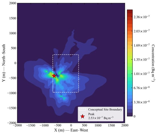
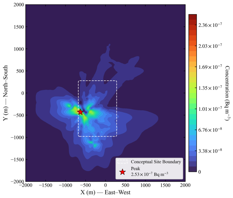
Figure 9 shows the spatial distribution characteristics of uranium aerosol activity concentration in the 2000 m × 2000 m area of the nuclear plant weighted by the annual meteorological joint frequency of 16 wind directions and six stability classes. The figure center coincides with the plant center. The concentration of uranium aerosol is found to be ranging from 0~2.53 × 10⁻⁷ Bq/m3.
Figure 9.
Spatial distribution of the joint-frequency-weighted expected uranium activity concentration over the 2000 m × 2000 m facility domain. The superposition calculation incorporates 16 wind directions, 6 wind speed classes, and 6 atmospheric stability classes based on the annual joint-frequency statistics. The generalized conceptual site boundary enclosing the stack sources is indicated by the white rounded dashed box.
The result shows that the uranium activity concentration presents an overall central concentrated distribution near the emission source. The peak of concentration is located at (x = −600 m, y = −500 m), which reaches 2.53 × 10⁻⁷ Bq/m3 and forms a high concentration hotspot area. Several sub-high concentration areas are located near the hotspot, with the activity concentration in the range of 1.70 × 10⁻⁷~2.37 × 10⁻⁷ Bq/m3.
The spatial dispersion of uranium aerosol shows obvious asymmetric multi-direction distribution characteristic. The uranium aerosol mostly disperses towards west (negative direction of x axis), south (negative direction of y axis) and northeast directions, where the diffusion distance on the west and south direction is the longest. An activity concentration >3.39 × 10⁻⁸ Bq/m3 can still be detected at 1300 m away on the east direction. On the west and south directions, the same concentration diffuses till about 1800 m and 1700 m range respectively. The diffusion on north direction is significantly shorter than the three other directions.
The attenuation characteristics of uranium activity concentration show that the concentrations decrease rapidly outward from the center of the hotspot: outside of 500 m of the hotspot area, the concentration decreases from the peak value 2.53 × 10⁻⁷ Bq/m3 to 3.39 × 10⁻⁸ Bq/m3; in the area beyond 1500 m, the concentration basically decreases to 1 × 10⁻⁹ Bq/m3, which is close to the environmental background level.
3.4. Comparison of Uranium Activity Concentration Distribution Between the Highest Frequency Scenario and Joint-Frequency Weighting
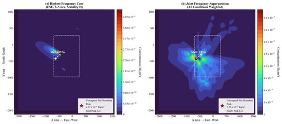
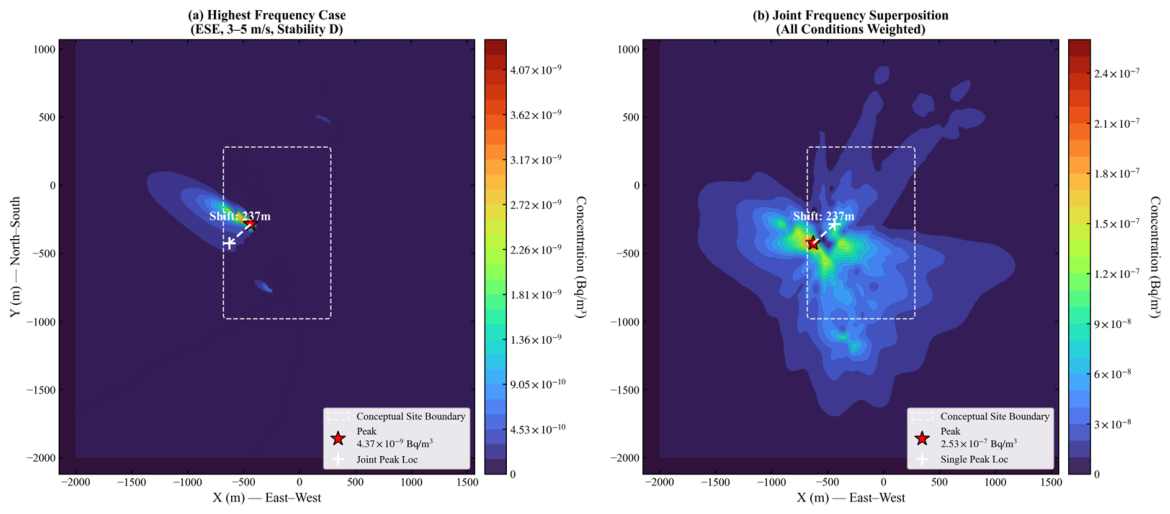
Figure 10 compares the uranium aerosol activity concentration field obtained from the single most-frequent meteorological condition (ESE wind direction, 3–5 m/s, Stability Class D) with the annual joint-frequency-weighted expected concentration field. The joint-frequency-weighted field represents the probability-weighted superposition of all wind-direction, wind speed, and stability-class combinations.
Figure 10.
Comparison of uranium aerosol activity concentrations and peak positions between (a) the single most-frequent meteorological bin (ESE, 3–5 m/s, stability class D) and (b) the annual expected field. Red stars mark the global peak concentration locations, and the dashed line indicates the 237 m peak-location shift (detailed coordinates are listed in Supplementary Table S2). The white rounded dashed boxes indicate the generalized conceptual site boundary.
Under the single most-frequent meteorological condition, the uranium aerosol activity concentration shows a near gaussian narrow band distribution aligned with the downwind direction of the ESE inflow. The peak concentration is 4.37 × 10⁻⁹ Bq/m3.
Under the joint-frequency-weighted scenario, the uranium aerosol activity concentration shows a multi-directional asymmetric distribution with a wider coverage and significant central agglomeration; the concentration peak is 2.53 × 10⁻⁷ Bq/m3, which is 58 times higher than the peak of the single most-frequent scenario, and the peak position shifts by 237 m to northeast direction relative to that of the single scenario.
These differences show that the single most-frequent meteorological condition does not fully represent the annual expected concentration pattern in this case study. However, because the single-scenario map is a conditional concentration field under one meteorological condition and the weighted map is an annual expected field, the peak ratio should be interpreted as a screening-level representativeness indicator rather than a direct time-resolved concentration ratio. The 237 m peak-location shift suggests a potential hotspot-position bias when only the most-frequent meteorological condition is used. Relative data of peak positions and activity concentrations are listed in Supplementary Table S2.
4. Discussion
4.1. Regulation Mechanism of Inlet Wind and Atmospheric Stability
4.1.1. Regulation Mechanism of Inlet Wind Velocity on Flow Field of Building Complex
In this study, the velocity difference between the windward and leeward sides of the buildings expanded continuously with the increase in inlet wind speed. The core mechanism lies in the coupling effect of incoming flow inertia and building bypass flow effect. Under high wind speed conditions, the inertial force of the incoming flow is significantly enhanced, leading to a stronger airflow blocking and acceleration effect on the windward side of the buildings. It induces simultaneously more intense flow separation and negative pressure wake zone on the leeward side, which ultimately amplifies the velocity difference between the two sides. This law confirms that even under high wind speed conditions, a stable low-velocity retention zone can still be formed on the leeward side of the buildings, providing weak dynamic conditions for the local accumulation of uranium aerosol. This contradicts the common assumption that pollutants become fully diffused under high wind speeds.
The overall wind velocity level attenuated continuously, which is caused by the cumulative effect of the underlying surface roughness of the building complex. The dissipation of incoming flow kinetic energy and turbulent wake interference caused by the front-row buildings continuously deteriorate the inflow conditions of the rear-row buildings. With the increase in row number, the blocking effect of the building complex on the near-surface airflow accumulates. This eventually leads to the overall flow field of the rear-row buildings being in a weak dynamic state. This result provides a possible explanation for the enhanced retention tendency in rear-row building areas.
4.1.2. Regulation Mechanism of Atmospheric Stability on Flow Field of Building Complex
When the atmospheric stability increased from Class A to Class F, the near-surface wind velocity showed a continuous attenuation trend, and the velocity difference between the windward and leeward sides decreased continuously. This is consistent with the turbulence developing theory in the atmospheric boundary layer: under unstable atmospheric conditions, the strong thermal convection drives sufficient downward momentum transport. The high-altitude momentum can be effectively transported downward, and the near-surface airflow has sufficient dynamic force. However, under stable atmospheric conditions, the thermal convection is inhibited. The near-surface airflow loses the supplement of high-altitude momentum. The whole system is in a weak flow state, and the dynamic difference between the windward and leeward sides of the buildings also disappears.
Particularly under Class F stable condition, the wind velocity in the valley regions of all building rows was close to 0 m/s, and the wind velocity in the whole section is basically maintained below 2 m/s, forming a large-scale static wind retention zone. This characteristic may contribute to localized airborne activity accumulation. Under weak turbulence conditions, atmospheric dilution is reduced, which may promote localized enrichment around building complexes, forming local radiation hotspots. This result is consistent with the concentration distribution law after joint-frequency weighting above: although the annual occurrence frequency of Class F high stability condition is low, it represents an unfavorable scenario where the suppression of vertical turbulent exchange leads to localized nuclide enrichment.
Based on the results of Figure 8, the coupled condition of low wind speed and high stability represents one of the most unfavorable simulated conditions, with weak near-surface flow field and elevated retention risk of radionuclides in the plant. From the perspective of the As Low As Reasonably Achievable (ALARA) principle of radiation protection, this conclusion could help inform the refined management and control of nuclear facilities: on the one hand, it is advisable to establish an emergency monitoring and source intensity control plan for the coupled condition of Class F stability and low wind speed, focusing on the occupational exposure level in the rear-row buildings and the leeward valley regions; on the other hand, in the environmental impact assessment of nuclear facilities, high stability conditions could be given greater emphasis as the key evaluation scenarios, rather than only using the conventional conditions of the highest frequency wind speed and stability, to reduce the possibility of under-representing unfavorable dispersion conditions of radioactive diffusion.
In addition, the flow field results of this study further indicate that building complex can modify near-surface diffusion and provide useful information for the monitoring layout in the nuclear facility plant. Additional monitoring points may be considered on the leeward side of the buildings, the wind velocity valley regions of the rear-row buildings, and the westward/southward dominant diffusion paths, rather than only evenly arranging monitoring points at the plant boundary, to realize accurate monitoring and early warning of radiation risks.
4.2. Formation Mechanism of Uranium Aerosol Spatial Distribution
In this study, weighted uranium activity concentration shows a central agglomeration distribution, with a hotspot near the plant center. This characteristic is consistent with atmosphere aerosol diffusion theory and retention effect of multi-row buildings in the plant. In the near-source central area, the air turbulence intensity is fully weakened by complex building layout, which attenuates the dilution and diffusion of uranium aerosol, resulting in a stable high-concentration area. This area may be considered a priority zone for occupational radiation protection of the nuclear plant.
The asymmetric multi-direction characteristic of uranium aerosol diffusion is a direct reflection of annual meteorological joint frequency. The dominant diffusion directions as west, south and east correspond to the three high-frequency directions (WSW, S, NNE). This indicates that the annual high-frequency wind directions directly determine the long-distance diffusion path of uranium aerosol. By contrast, the diffusion on north direction is limited, which is related to the low frequency of corresponding wind direction and the shielding effect of buildings. This result confirms that the weighted simulations based on joint frequency can reliably reproduce the average diffusion of aerosols under annual meteorological conditions and avoids the directional deviation of simulation of typical single case.
Uranium activity concentration declines rapidly from the plant center outward. It is notable that the fast decrease section within 500 m is the important region that the nuclide concentration drops from the peak to a low level. This is also the key section of environmental monitoring points in the nuclear facility. The section beyond 1500 m reaches background level.
Under the ALARA principle of radiation protection, these findings could help with refined radiation control of nuclear bases: First, the radiation control may be enforced for the hotspot areas in the central site, with optimization of ventilation and radiation shielding. Second, long-term environmental monitoring points could be set up along the three dominant diffusion paths on the east, south and west directions, focusing on the change in concentrations of site boundaries under high frequency wind directions. Meanwhile, the emergency monitoring plan may be improved to achieve preliminary information for further dose-informed assessment.
The distribution result also verifies the engineering applicability of the joint-frequency weighting method adopted in this study. Compared with the symmetric diffusion results of traditional single condition simulation, the multi-directional asymmetric simulation can provide more realistic basic data for environmental impact assessments and the radiation dose estimation of nuclear facilities.
4.3. Differences Between Single-Scenario and Joint-Frequency Weighting Methods and Their Nuclear Safety Implications
The comparison between the single most-frequent meteorological bin and the joint-frequency-weighted field highlights the representativeness limitation of using one selected scenario for annual hotspot screening. The single-scenario simulation describes the dispersion pattern conditional on ESE wind direction, 3–5 m/s wind speed, and stability class D. By contrast, the joint-frequency-weighted field represents the annual expected concentration obtained by superposing all simulated meteorological combination. This suggest that the comparison may be interpreted as an assessment of how much information may be lost when annual meteorological variability is reduced to one representative condition.
The broader footprint and shifted peak position in the joint-frequency-weighted field are mainly caused by the combined effects of wind-direction variability, stability-dependent vertical mixing, and building-induced flow modification. Although the most-frequent bin contributes to the annual distribution, other meteorological combinations can generate higher local concentrations or transport pollutants toward different sectors. As a result, the annual expected hotspot does not necessarily coincide with the hotspot predicted by the single most-frequent scenario. In this case study, the peak position differs by 237 m, indicating that hotspot identification based only on the most-frequent meteorological condition may be spatially biased.
The higher global expected peak in the joint-frequency-weighted field suggests that the single most-frequent scenario may under-represent some annual screening indicators in this specific case, including peak concentration and hotspot location. The joint-frequency approach is best regarded as a probabilistic screening tool that complements, rather than replaces, selected deterministic scenarios for environmental monitoring layout and radiation-protection assessment.
4.4. Model Assumptions, Limitations, and Transferability
In this study, uranium aerosol is represented as a passive tracer without dry/wet deposition or radioactive decay. This treatment is based on the assumption that gaseous effluents are discharged after HEPA filtration systems and cooling, so that the released particulate fraction is dominated by fine or sub-micron aerosols and the discharge temperature is close to ambient conditions [24]. For such small particles, the gravitational settling velocity and deposition rate are low enough, making their transport behavior resemble that of a passive gas in the near field [25]. Under these microscale conditions, treating the aerosol as a passive tracer is a standard and conservative screening-level assumption widely adopted in near-field radionuclide dispersion CFD studies [1,2]. Emissions are modeled as cold sub-micron releases without thermal buoyancy. Each meteorological combination is simulated under steady-state conditions, since facility ventilation and cooling processes reduce the effluent temperature to near-ambient conditions before discharge. However, these assumptions may overestimate near-field and far-field activity concentrations relative to deposition- and decay-inclusive assessments and should be regarded as screening-level unless extended. The workflow is transferable to other nuclear facilities, but joint frequencies, source terms, building layouts, and boundary conditions must be re-established for each site.
The reported concentration fields are deterministic CFD results under prescribed source-term, meteorological, boundary-condition, and turbulence-model assumptions. Major uncertainty sources include turbulence-model closure, inlet wind-profile specification, meteorological classification, passive-scalar treatment, neglected deposition and decay, and steady-state RANS limitations. Numerical robustness was partly supported by the grid-independence test, in which the ground-level peak concentration changed by less than 1% when the mesh exceeded 2.6 million elements. The wind-tunnel comparison also provides preliminary support for the selected computational settings, although it covers only one meteorological scenario and does not constitute full uncertainty quantification.
The comparison with the single most-frequent meteorological scenario is used to evaluate the representativeness of a commonly used simplified screening approach. It is not intended to establish general superiority over all conventional dispersion models. Gaussian-plume, Lagrangian, and regulatory dose-assessment methods remain important references for long-term compliance assessment, and full benchmarking against these approaches should be conducted in future work. Therefore, the proposed workflow should be regarded as a building-resolved, joint-frequency-weighted screening tool. Practical radiation-protection management and monitoring layout require additional site-specific validation, source-term confirmation, and deposition/d dose-inclusive assessment.
5. Conclusions
This study addresses the insufficient representativeness of traditional single-scenario methods in atmospheric diffusion simulation of nuclear facility gaseous effluents. A CFD numerical simulation framework based on annual meteorological joint-frequency weighting is constructed, and the flow field characteristics of the plant building complex and uranium aerosol diffusion law are analyzed. The main conclusions are as follows:
- (1)
- The near-surface flow field of the plant is regulated by inlet wind velocity, atmospheric stability, and building layout. High wind speed significantly amplifies the wind velocity difference between the windward and leeward sides of buildings. Class F high stability conditions and rear-row building areas are prone to form large-scale low-velocity retention zones, which represent unfavorable simulated conditions for localized radionuclide accumulation.
- (2)
- The uranium aerosol concentration field weighted by joint frequency presents a distinct distribution characteristic of central agglomeration and asymmetric gradient attenuation. Westward, southward and northeastward are the annual dominant diffusion paths, which generally correspond to the annual high-frequency wind directions.
- (3)
- Relative to a single most-frequent meteorological simulation, joint-frequency weighting yields a broader multi-directional footprint, a higher global expected peak, and a 237 m shift in hotspot location in the illustrative case study. The framework may help to bridge deterministic building-resolved CFD with probabilistic meteorological weighting and may support monitoring layout screening when combined with validation and dose assessment.
- (4)
- The practical implications of these results should be interpreted with caution. The present study provides a building-resolved, joint-frequency-weighted CFD screening framework, but it does not provide a full uncertainty quantification or a benchmark against all conventional dispersion assessment methods. Further comparison with Gaussian-plume, Lagrangian, and regulatory dose-assessment models, together with additional field or wind-tunnel validation, is needed before applying the results to site-specific radiation-protection decisions.
Supplementary Materials
The following supporting information can be downloaded at https://www.mdpi.com/article/10.3390/app16136780/s1. Table S1: Joint frequency. Table S2: Figure 10 comparison.
Author Contributions
Conceptualization, J.C. and J.K.; methodology, J.C.; software, J.C.; validation, B.L. and S.C.; formal analysis, J.C. and F.W.; investigation, F.W.; resources, J.K.; data curation, F.W.; writing—original draft preparation, J.C.; writing—review and editing, J.K.; supervision, J.K. and B.L.; funding acquisition, J.K. and B.L. All authors have read and agreed to the published version of the manuscript.
Funding
This work was supported by the Study on the Radiation Environmental Suitability of the Medical Isotope Production Base in Shanxi Province (Grant No. 202304041101050) and Study on Radiation Environmental Capacity and Optimized Radioactive Discharge for Large-Scale Nuclear Bases (CNNC-JCYJ-202340).
Institutional Review Board Statement
Not applicable.
Informed Consent Statement
Not applicable.
Data Availability Statement
Joint-frequency data are provided in Supplementary Table S1. Large scenario-wise concentration grids are available from the corresponding author on reasonable request.
Acknowledgments
During the preparation of this manuscript/study, the author(s) used Doubao version 2.1 (AI assistant developed by ByteDance, No. 6, Zhichun Road, Haidian District, Beijing, P.R.China) for the purposes of linguistic polishing. The authors have reviewed and edited the output and take full responsibility for the content of this publication.
Conflicts of Interest
The authors declare no conflicts of interest.
Abbreviations
The following abbreviations are used in this manuscript:
| ALARA | As Low As Reasonably Achievable |
| CFD | Computational fluid dynamics |
| HEPA | High-Efficiency Particulate Air |
| TDS | Transport of Diluted Species |
References
- Li, Z.; Ye, Y.; Liu, X.; Wang, Z. Downscaled Simulation Approach for Near-Field Nuclear Facility Pollutant Atmospheric Transport and Dispersion Using a Coupled WRF–CFD Downscaling Model Framework. J. Environ. Radioact. 2026, 292, 107864. [Google Scholar] [CrossRef] [Scilit] [PubMed]
- De Sampaio, P.A.B.; Junior, M.A.G.; Lapa, C.M.F. A CFD Approach to the Atmospheric Dispersion of Radionuclides in the Vicinity of NPPs. Nucl. Eng. Des. 2008, 238, 250–273. [Google Scholar] [CrossRef] [Scilit]
- Wang, Z.; Ding, D.; Dou, X.; Li, Z. Effects of Improved Atmospheric Boundary Layer Inlet Boundary Conditions for Uneven Terrain on Pollutant Dispersion from Nuclear Facilities. Atmosphere 2025, 16, 1203. [Google Scholar] [CrossRef] [Scilit]
- Sinha, V.; Atikler, M.; Mileski, M. Atmospheric Dispersion of Radioactive Materials for Radiological Risk Assessment in Case of Hypothetical Sodium Cooled Fast Reactor Accident. Nucl. Eng. Des. 2024, 422, 113124. [Google Scholar] [CrossRef] [Scilit]
- Baklanov, A.; Sørensen, J.H.; Mahura, A. Methodology for Probabilistic Atmospheric Studies Using Long-Term Dispersion Modelling. Environ. Model. Assess. 2008, 13, 541–552. [Google Scholar] [CrossRef] [Scilit]
- U.S. Nuclear Regulatory Commission. Regulatory Guide 1.111, Revision 1: Methods for Estimating Atmospheric Transport and Dispersion of Gaseous Effluents in Routine Releases from Light-Water-Cooled Reactors; U.S. Nuclear Regulatory Commission: Washington, DC, USA, 1977.
- Nakayama, H.; Jurcakova, K.; Nagai, H. Development of Local-Scale High-Resolution Atmospheric Dispersion Model Using Large-Eddy Simulation. Part 3: Turbulent Flow and Plume Dispersion in Building Arrays. J. Nucl. Sci. Technol. 2013, 50, 503–519. [Google Scholar] [CrossRef] [Scilit]
- Liu, S.; Chan, T.L. A Coupled CFD-Monte Carlo Method for Simulating Complex Aerosol Dynamics in Turbulent Flows. Aerosol Sci. Technol. 2017, 51, 269–281. [Google Scholar] [CrossRef] [Scilit]
- Martín, F.; Janssen, S.; Rodrigues, V.; Sousa, J.; Santiago, J.L.; Rivas, E.; Stocker, J.; Jackson, R.; Russo, F.; Villani, M.G.; et al. Using Dispersion Models at Microscale to Assess Long-Term Air Pollution in Urban Hotspots: A FAIRMODE Joint Intercomparison Exercise for a Case Study in Antwerp. Sci. Total Environ. 2024, 925, 171761. [Google Scholar] [CrossRef] [Scilit] [PubMed]
- Tominaga, Y. CFD Simulations of Turbulent Flow and Dispersion in Built Environment: A Perspective Review. J. Wind Eng. Ind. Aerodyn. 2024, 249, 105741. [Google Scholar] [CrossRef] [Scilit]
- Smith, B.L.; Andreani, M.; Bieder, U.; Bestion, D.; Ducros, F.; Graffard, E.; Heitsch, M.; Scheuerer, M.; Henriksson, M.; Hoehne, T.; et al. Assessment of Computational Fluid Dynamics (CFD) for Nuclear Reactor Safety Problems; NEA/CSNI/R(2007)13; OECD Nuclear Energy Agency: Paris, France, 2008. [Google Scholar]
- Tang, B.; Wang, H.; Xu, J.; Lin, J.; Hu, J.; Chen, R. High-Resolution Simulation of the Near-Field Pollutant Dispersion in a Nuclear Power Plant Community with High-Performance Computing. J. Nonlinear Math. Phys. 2024, 31, 6. [Google Scholar] [CrossRef] [Scilit]
- Fiates, J.; Vianna, S.S.V. Numerical Modelling of Gas Dispersion Using OpenFOAM. Process Saf. Environ. Prot. 2016, 104, 277–293. [Google Scholar] [CrossRef] [Scilit]
- Liu, Y.S.; Cui, G.X.; Wang, Z.S.; Zhang, Z.S. Large Eddy Simulation of Wind Field and Pollutant Dispersion in Downtown Macao. Atmos. Environ. 2011, 45, 2849–2859. [Google Scholar] [CrossRef] [Scilit]
- Vardoulakis, S.; Fisher, B.E.A.; Pericleous, K.; Gonzalez-Flesca, N. Modelling Air Quality in Street Canyons: A Review. Atmos. Environ. 2003, 37, 155–182. [Google Scholar] [CrossRef] [Scilit]
- Gousseau, P.; Blocken, B.; Stathopoulos, T.; Van Heijst, G.J.F. Near-Field Pollutant Dispersion in an Actual Urban Area: Analysis of the Mass Transport Mechanism by High-Resolution Large Eddy Simulations. Comput. Fluids 2015, 114, 151–162. [Google Scholar] [CrossRef] [Scilit]
- Tominaga, Y.; Stathopoulos, T. Numerical simulation of dispersion around an isolated cubic building: Comparison of various RANS models. Atmos. Environ. 2009, 43, 3200–3210. [Google Scholar] [CrossRef] [Scilit]
- Gousseau, S.; Blocken, B.; Stathopoulos, T.; van Heijst, G.J.F. CFD simulation of near-field pollutant dispersion on a high-resolution grid: Comparison with wind tunnel measurements for a building group. Atmos. Environ. 2011, 45, 428–440. [Google Scholar] [CrossRef] [Scilit]
- Tominaga, Y.; Stathopoulos, T. CFD simulation of near-field pollutant dispersion in the urban environment: A review of state-of-the-art. Atmos. Environ. 2013, 79, 752–773. [Google Scholar] [CrossRef] [Scilit]
- Chang, J.C.; Hanna, S.R. Air quality model performance evaluation. Meteorol. Atmos. Phys. 2004, 87, 167–196. [Google Scholar] [CrossRef] [Scilit]
- Shih, T.-H.; Liou, W.W.; Shabbir, A.; Yang, Z.; Zhu, J. A new k-ε eddy-viscosity model for high Reynolds number turbulent flows—Model development and validation. Comput. Fluids 1995, 24, 227–238. [Google Scholar] [CrossRef] [Scilit]
- GB/T 13201-91; Technical Methods for Making Local Emission Standards of Air Pollutants. Standards Press of China: Beijing, China, 1991.
- Tominaga, Y.; Stathopoulos, T. Turbulent Schmidt numbers for CFD analysis with various types of flowfield. Atmos. Environ. 2007, 41, 8091–8107. [Google Scholar] [CrossRef] [Scilit]
- DOE-STD-3020-2015; Specification for HEPA Filters Used by DOE Contractors. U.S. Department of Energy: Washington, DC, USA, 2015.
- Farmer, D.K.; Boedicker, E.K.; DeBolt, H.M. Dry deposition of atmospheric aerosols: Approaches, observations, and mechanisms. Annu. Rev. Phys. Chem. 2021, 72, 375–397. [Google Scholar] [CrossRef] [Scilit] [PubMed]

Disclaimer/Publisher’s Note: The statements, opinions and data contained in all publications are solely those of the individual author(s) and contributor(s) and not of MDPI and/or the editor(s). MDPI and/or the editor(s) disclaim responsibility for any injury to people or property resulting from any ideas, methods, instructions or products referred to in the content. |
© 2026 by the authors. Licensee MDPI, Basel, Switzerland. This article is an open access article distributed under the terms and conditions of the Creative Commons Attribution (CC BY) license.