


Abstract
Automated damage inspection of railway viaducts requires pixel-level identification of structural components and surface damage such as cracking and rebar exposure. A common assumption in bridge inspection is that damage segmentation improves when component information is provided alongside the image. This study tests that assumption on the Tokaido synthetic viaduct dataset using controlled comparisons between segmentation models with and without component information. Both damage and structural component segmentation are evaluated across multiple architectures, and the trained component model is assessed on real viaduct photographs against a baseline model requiring no task-specific training. Under the original random split, explicit component conditioning does not produce a measurable improvement in damage segmentation: all tested strategies remain within 0.008 mean Intersection-over-Union (mIoU) of a baseline without component input, and this null result persists even when component predictions are reliable. Under a leakage-controlled scene-disjoint split, however, the same component-aware variants show a small positive trend (up to mIoU over three seeds), so the effect of component conditioning depends on the evaluation protocol. The best unconditioned model reaches 0.569 mIoU for damage segmentation; for real-photo component segmentation, the trained model reaches 0.424 mIoU compared with 0.250 mIoU for the training-free baseline. These results show that multitask benefits reported in bridge inspection do not automatically translate into gains from explicit use of component information on synthetic viaduct data, where damage occurs almost exclusively on columns yet is too sparse for structural element identity to yield more than a marginal localisation gain. The multi-architecture benchmark and the measured real-photo structural transfer gap provide reference baselines for subsequent work on component-aware and transfer-robust inspection.
1. Introduction
Railway viaduct inspection requires pixel-level information about both structural components and visible surface damage. Manual visual inspection remains costly, time-consuming, and dependent on subjective interpretation, especially when elevated structures must be assessed repeatedly across large transport networks [1,2,3]. Semantic segmentation offers a direct route from inspection imagery to spatially explicit component and damage maps, but its usefulness depends on whether models can identify small damage regions and transfer beyond the data used for training. These requirements make viaduct inspection a stringent test case for modern segmentation methods.
Recent bridge-inspection research has established two important directions. First, bridge element parsing and defect segmentation can be learned jointly, and multitask models are often reported to improve element or defect metrics relative to single-task baselines [2,3]. Second, synthetic environments, such as the Tokaido synthetic viaduct benchmark and related synthetic inspection datasets [4,5,6], can reduce annotation cost and support repeatable experiments. These studies show that component information, synthetic data, and deep segmentation architectures can support structural inspection. They do not, however, resolve the issue of whether explicit component conditioning improves damage localisation under a controlled viaduct benchmark.
The distinction between multitask learning and explicit component conditioning is central to this study. A multitask network may improve damage segmentation because shared features regularise the encoder, because component supervision improves structural representation, or because the damage branch directly receives component information. Prior bridge-inspection work has mostly evaluated the combined effect of feature sharing and task interaction [2,3]. The practical question remains narrower: if a model already has access to an image, does adding predicted component information help it localise cracks, concrete damage, or exposed reinforcement? This question is testable only when architecture, training recipe, dataset split, and evaluation protocol are controlled.
Architecture choice adds a second unresolved factor. General semantic-segmentation research has moved from convolutional encoder–decoder models such as U-Net and DeepLabV3+ toward hierarchical transformers and modernised convolutional architectures, including Swin Transformer, SegFormer, and ConvNeXt [7,8,9,10,11,12,13,14]. Inspection imagery differs from generic scene parsing because damage classes are sparse, thin, and texture-driven. A model that performs well on broad segmentation benchmarks may therefore fail under strong foreground–background imbalance. A controlled comparison across convolutional neural network (CNN), ConvNeXt, Vision Transformer (ViT), SegFormer, and Swin-style architectures is needed before claims about the benefits of component-aware damage localisation can be interpreted.
Synthetic-to-real transfer also remains a limiting condition for real-life deployment. The Tokaido dataset provides controlled synthetic viaduct imagery with component and damage annotations, while dacl10k and related bridge datasets demonstrate the diversity and difficulty of real inspection photographs [4,15]. Foundation segmentation models provide a complementary reference point because GroundingDINO and the Segment Anything Model (SAM) can produce zero-shot masks without task-specific training [16,17]. Comparing a trained synthetic-data model against such a training-free baseline helps separate ordinary segmentation accuracy from real-photo transfer performance.
This study evaluates railway viaduct component and damage segmentation under a controlled benchmark design. Seven segmentation architectures are trained for structural component and damage segmentation on the Tokaido synthetic dataset, using fixed splits, repeated seeds, and a common evaluation protocol. A separate component-aware ablation study tests damage-only, parallel-head, hard-mask, detached soft-conditioning, and end-to-end soft-conditioning variants. The design isolates whether component predictions improve damage localisation beyond a damage-only baseline. The best damage model reaches foreground mIoU on the synthetic test split, while the component-aware variants remain within mIoU of the unconditioned baseline. Under this random split, the component-aware variants provide no measurable damage segmentation gain; under a leakage-controlled scene-disjoint split, however, the same variants show a small positive trend, so the effect of component conditioning is protocol-dependent.
The paper makes three contributions. First, the study provides a controlled CNN–Transformer benchmark for viaduct structural component and damage segmentation on the Tokaido dataset. Second, the component-aware ablation shows that the effect of reliable component predictions on damage localisation is protocol-dependent: absent under the original random split, with a small positive trend under a leakage-controlled scene-disjoint split. Third, the real-photo component-transfer evaluation compares a component segmentation model trained on synthetic data with a GroundingDINO + SAM zero-shot pipeline (GroundedSAM), where the trained model reaches mIoU and the zero-shot baseline reaches mIoU on real viaduct photographs. Together, these results position the benefits of component-aware conditioning as an empirical question rather than an assumed benefit, and they provide baseline evidence for future transfer-robust inspection models.
2. Related Work
Research on automated bridge and viaduct inspection draws from two distinct but interacting bodies of literature: generic semantic segmentation, which supplies the backbone architectures and training methods, and inspection-specific segmentation, which defines the tasks, datasets, and domain challenges. Progress in generic segmentation has been rapid and architecturally diverse, while progress in inspection-specific methods has been constrained by small real-world datasets, heterogeneous evaluation protocols, and narrow damage taxonomies. This section reviews both areas with respect to the three unresolved questions that motivate the present study: how convolutional neural network (CNN) and transformer architectures compare on the same viaduct benchmark, whether explicit component-label conditioning improves damage localisation, and how large the synthetic-to-real transfer gap is against a training-free baseline.
2.1. Semantic Segmentation Architectures for Structural Inspection
The encoder–decoder paradigm, established by U-Net [7] and its densely connected extension UNet++ [18], defined the spatial segmentation baseline: a contracting encoder captures context and a symmetric decoder recovers spatial resolution through skip connections. DeepLabv3+ [8] offered a complementary approach via atrous spatial pyramid pooling, capturing multi-scale context without the resolution loss of pooling. UPerNet [19] paired a feature pyramid network with a pyramid pooling module over any hierarchical backbone, and it is the primary decoder used with Swin Transformer and ConvNeXt in the present benchmark. These convolutional baselines are well validated for bridge crack and damage segmentation tasks [20,21,22,23,24,25,26] and represent the CNN family in the controlled comparison.
Vision Transformer architectures introduced global self-attention and altered the accuracy–efficiency tradeoff [27,28,29]. Swin Transformer [9] achieved 48.1 mIoU on ADE20K with the UPerNet decoder by using shifted window attention to build hierarchical feature maps. SegFormer [10] combined a mix-transformer hierarchical encoder with a lightweight all-multilayer-perceptron (MLP) decoder, reaching 51.0/51.8 mIoU (single-/multi-scale). ConvNeXt [11] demonstrated that a convolutional network redesigned with transformer principles—large kernels, inverted bottleneck, and layer normalisation—matches Swin Transformer at comparable scale (44.4 vs. 44.5 mIoU). This result showed that self-attention is not strictly necessary for competitive dense segmentation and motivates treating CNN and transformer families as peers under controlled comparison rather than as successive generations.
Applied to inspection-specific tasks, the advantage of transformers over CNNs is inconsistent [30,31]. TransUNet improves over U-Net and DeepLabv3+ by at least 3.8% mIoU on concrete crack datasets [32], suggesting that global attention helps localise thin crack features. However, the CCSNet ablation [21] reveals that the transformer branch alone drops to 52.61% mIoU on a three-class concrete damage task, well below the CNN branch at 76.13%; only their combination reaches 82.74%. MixSegNet [33] and ETCS-Net [34] report similar patterns: hybrid CNN-Transformer designs outperform either family in isolation for crack and multiclass damage segmentation [35,36,37,38,39,40]. Because existing inspection papers use heterogeneous datasets and training protocols, the relative ranking of architecture families on a common viaduct benchmark remains an open empirical question. Using the Tokaido benchmark, Roy et al. [41] demonstrate the superior performance of transformer-based architectures, showing that the SegFormer (MiT-B5) model significantly outperforms conventional U-Net and Attention U-Net baselines in both structural component and damage detection tasks.
2.2. Bridge Component Segmentation and Multitask Inspection
Bridge element parsing originated as component classification [1] and evolved into pixel-level component segmentation [42,43,44], enabling spatial attribution of damage to specific structural elements. The dominant framework became multitask learning [45], in which a shared encoder is jointly supervised on component and damage targets, motivated by the expectation that component identity provides a structural prior for damage localisation.
The reported multitask evidence is quantitatively consistent. Zhang et al. [2] compare twelve multitask design variants on a 145-image Virginia DOT bridge dataset. The best variant improves bridge element mIoU from 82.89% to 85.48% and corrosion mIoU from 80.85% to 83.31% over single-task baselines while also reducing total training time. AECIF-Net [3] replaces simple feature sharing with bidirectional cross-task co-attention between task-specific relearning subnets. The model achieves 92.11% element mIoU and 87.16% defect mIoU on SBCIV, improving over naive multitask learning by 2.51% and 1.90% respectively. Yao et al. [6] validate joint component and crack segmentation on high-rise building images, achieving component F-scores above 92% and a crack F-score 73.51% under a synthetic-trained DeepLabv3+ model.
The studies above do not establish whether the reported performance gain obtained by multitask training arises from shared-encoder regularisation, from richer structural feature representations, or from explicit routing of component information into the damage branch. All three studies train a shared encoder jointly; none isolate the conditioning signal by providing component predictions as an explicit input to a damage-only encoder. Because the present study asks precisely this question, the multitask literature provides the motivating context but not the answer.
2.3. Synthetic Inspection Data and Domain Transfer
Manually annotating real inspection images is expensive and inconsistent: lighting, viewpoint, surface texture, and damage morphology vary widely, and expert labellers are scarce. The choice of imaging modality further affects segmentation performance [46,47]. Synthetic rendering offers a scalable alternative. The Tokaido dataset [4] renders Tokaido Shinkansen viaducts from 3D CG models under varied lighting, weather, and damage states, producing pixel-accurate component and damage annotations without manual labelling. Zarski et al. [5] apply a comparable approach to post-earthquake building inspection, achieving component mIoU 91.54% on synthetic test data. Crack and exposed-rebar IoU remain near 30% because label overlap and class imbalance are not resolved by the synthetic rendering alone, and the authors explicitly note that real-world fine-tuning is required. Yao et al. [6] generate 2000 photorealistic building images using a physics-based crack plugin, reaching component F-scores above 92% and crack F-score 73.51%, with the synthetic model successfully identifying over 96% of real field images. Rahman et al. [48] target bridge damage transfer directly but do not report standardised mIoU transfer metrics. Addressing the domain shift inherent in heritage structures, Fallahy and Rezazadeh [49] introduce MARBLE-DA, a label-free unsupervised domain-adaptation framework that combines Sobel-edge preprocessing with adaptive batch normalisation to enable robust crack detection in masonry without requiring target-domain annotations.
These studies share a common limitation: the magnitude of the synthetic-to-real performance drop is reported inconsistently, measured on private test sets, or not reported at all. dacl10k [15,50], a 9920-image real bridge-inspection benchmark with 12 damage and six component classes, provides the standardised evaluation domain needed to measure transfer consistently, but dacl10k has not previously been used as the target for Tokaido-trained models. The dacl10k taxonomy covers 12 damage classes with a different labelling convention from Tokaido’s two-class damage scheme (concrete surface damage; ExposedRebar); mapping the two taxonomies would require annotation re-labelling beyond the scope of this study. The 16 hand-annotated real viaduct photographs used here provide a smaller but taxonomy-compatible transfer target. Promptable foundation models offer a complementary reference point. GroundingDINO + SAM [16,17] produces text-prompted segmentation without task-specific training and is used here as a zero-shot lower bound. Parameter-efficient foundation-model adaptation is also viable: low-rank adaptation (LoRA) of SAM achieves mask average precision () and mIoU on a masonry crack dataset [51], demonstrating that fine-tuning can close the gap to task-specific segmentation. Fine-tuned adaptation and zero-shot deployment differ fundamentally in data requirements, however, and the zero-shot protocol is the appropriate baseline for measuring how much task-specific synthetic training contributes.
Collectively, the existing literature establishes that hybrid CNN-Transformer designs outperform single-architecture baselines for damage segmentation, that multitask bridge inspection is broadly beneficial, and that synthetic environments can support inspection-relevant segmentation. Three questions remain unresolved under controlled conditions: whether architecture family determines performance on a standardised viaduct benchmark, whether explicit component-label conditioning provides damage segmentation gains beyond shared-encoder supervision, and what the synthetic-to-real component segmentation gap is relative to a training-free zero-shot baseline on real viaduct photographs.
3. Methodology
This section defines the segmentation tasks, implemented model families, component-aware conditioning variants, and training configuration used throughout the benchmark reported in the present paper. The study is both a controlled architecture benchmark and an ablation study design: standard segmentation architectures are compared under the same conditions, while the component-aware variants constitute the conditioning interventions used to test whether structural component information helps damage localisation.
3.1. Task Formulation and Label Spaces
Each input image is a red–green–blue (RGB) viaduct rendering , resized and cropped to before being passed to the network. Two dense prediction tasks are considered. The structural component task predicts one of five labels at each pixel: nonbridge, slab, beam, column, or nonstructural. The last class, nonstructural, aggregates minor structural elements (rail, sleeper, and other non-load-bearing parts); the merging uses zero-based indices after label conversion (see Section 3.2). The damage task predicts one of three labels: nondamage, concrete, or ExposedRebar. The single-task models output one logit tensor for the selected task, with for component segmentation and for damage segmentation.
Performance is optimised and monitored using foreground mean Intersection-over-Union (mIoU), denoted , where Intersection-over-Union (IoU) is computed per class before averaging. This metric excludes the dominant background class, nonbridge for component segmentation and nondamage for damage segmentation, so that model selection is driven by the structural and damage classes that determine inspection usefulness. The same foreground convention is used by the validation scheduler and by the checkpoint criterion.
3.2. Dataset
Both tasks are trained and evaluated on the Tokaido dataset [4], a synthetic photorealistic collection of 7575 viaduct images rendered from three-dimensional bridge models using the open-source Blender3D modelling tool (version 4.3.2; Blender Foundation, Amsterdam, The Netherlands). A viaduct is a multi-span elevated bridge structure, typically used to carry railways or roads over valleys or urban areas. The images are representative of UAV-acquired aerial imagery and come with pixel-accurate ground-truth annotations stored as unsigned-integer label images. Each sample includes segmentation masks covering structural object types—slab (the flat horizontal deck that forms the roadway or rail bed), beam (longitudinal load-bearing members that span between supports), column (vertical pillars that carry the beam loads to the ground), rail and sleeper (railway track components), and other minor elements—as well as two damage categories: concrete surface damage (cracking and spalling visible on the surface) and exposed rebar (severe deterioration where steel reinforcing bars have become visible due to cover loss or corrosion).
A validity flag stored in the file-list CSV is used to exclude low-quality or incomplete samples prior to any split; files whose label images are missing from disk are additionally filtered out. Figure 1 shows representative examples of the input images and their ground-truth annotations.
Figure 1.
Representative samples from the Tokaido synthetic dataset (test split). Each row shows the RGB image (left), component ground-truth mask (centre; slab = red, beam = green, column = blue, nonstructural = yellow-orange, nonbridge = dark grey), and damage ground-truth mask (right; concrete = red, ExposedRebar = green, and nondamage = dark grey). Rows 1–3 are selected to show abundant damage pixels from both foreground classes; rows 4–6 cover all structural component classes. Outside the selected rows, damage pixels are typically sparse and localised on structural surfaces, reflecting the severe class imbalance addressed by the imbalance-aware loss functions.
Class Indexing and Label Merging
Raw label images store class indices as unsigned integers starting at 1; the preprocessing pipeline subtracts 1 to obtain zero-based indices in the range 0–7 before merging. For the component task, zero-based source classes 5, 6, and 7—corresponding to raw classes 6 (rail), 7 (sleeper), and 8 (other minor elements)—are merged into the nonstructural class at zero-based index 4. Raw class 5 already maps to nonstructural and is not a merge source. The merge reduces the eight raw component labels to five training classes.
3.3. Preprocessing and Augmentation
All images follow a common preprocessing pipeline before tensor conversion. For training, the image is first scaled with LongestMaxSize so that the longer side matches the configured training size and is then padded with zeros using PadIfNeeded until the canvas is obtained. A random crop is then extracted. Training augmentation consists of horizontal flipping with probability , random brightness–contrast perturbation with probability , and Gaussian blur with probability , followed by normalisation and ToTensorV2. For non-augmented evaluation transforms, the same longest-side scaling, zero padding, normalisation, and tensor conversion are used without random crop or photometric augmentation. The same resize–pad–normalise convention is used for both component and damage inputs, ensuring that task differences arise from labels and model heads rather than from preprocessing.
3.4. Single-Task Segmentation Architectures
The single-task benchmark evaluates seven segmentation architectures under the same task interface. Three models use segmentation_models_pytorch decoders with an ImageNet-pretrained timm-efficientnet-b3 encoder: U-Net [7], UNet++ [18], and DeepLabV3+ [8]. U-Net provides the basic encoder–decoder baseline with skip connections; UNet++ adds nested skip pathways to reduce the semantic gap between encoder and decoder features; and DeepLabV3+ replaces the symmetric decoder with atrous spatial pyramid pooling and a lightweight refinement decoder. Their verified trainable parameter counts are 13.16 million, 13.63 million, and 11.68 million, respectively.
The remaining four models use custom wrappers around timm encoders and decoder heads. ViT-Seg uses vit_base_patch16_224 [52] with a UPerNet-style decoder [19]; intermediate transformer blocks are reshaped into spatial feature maps and fused at one-quarter input resolution. ConvNeXt-Seg uses convnext_base [11] as a four-stage feature encoder with the same UPerNet-style decoder. SegFormer uses a Pyramid Vision Transformer v2 (PVT v2) pvt_v2_b2 hierarchical encoder with a SegFormer-style multilayer-perceptron (MLP) decoder [10]; each stage is projected to a common channel dimension, upsampled to one-quarter resolution, concatenated, and fused before the segmentation head. Swin-UPerNet uses swin_base_patch4_window7_224 [9] with the UPerNet-style decoder. The verified trainable parameter counts are 93.12 million for ViT-Seg, 93.37 million for ConvNeXt-Seg, 25.97 million for SegFormer, and 92.12 million for Swin-UPerNet.
UPerNet Decoder
The shared UPerNet decoder used by ViT-Seg, ConvNeXt-Seg, and Swin-UPerNet consists of (i) per-level lateral convolutions that project all feature maps to a common -dimensional space, (ii) a feature pyramid network (FPN) top-down pathway that adds upsampled deeper features to shallower ones, (iii) convolutional refinement on each level, and (iv) a final fusion step that upsamples all levels to a common resolution, concatenates them, and applies a further convolution. The segmentation head consists of a Conv-BN-ReLU block followed by a convolution that produces the C-channel logit map, which is upsampled to the original image resolution using bilinear interpolation.
3.5. Component-Aware Damage Segmentation
The component-aware multitask model uses a shared convnext_base encoder and task-specific UPerNet-style decoder branches. The component branch produces a feature map at one-quarter input resolution and component logits ; the damage branch produces a damage feature map and damage logits . When conditioning is active, the damage feature map is concatenated with a component-derived conditioning tensor and passed through a single Conv-BN-ReLU fusion block before the damage head. The input channel count is for the hard-mask variant (one-hot over five component classes) and for the soft variants (full feature map); in both cases the output is projected back to 256 channels. Figure 2 shows the shared encoder, task branches, and optional conditioning route.
Figure 2.
Component-aware damage segmentation architecture. The shared ConvNeXt encoder produces multi-scale features F fed to both branches. The component branch (top) computes feature map and logits ; the damage branch (bottom) fuses with the conditioning tensor before the damage head. The five conditioning modes differ in how is formed (see legend); in the damage-only and parallel-head modes, the dashed conditioning path is absent. The subscript denotes trainable parameters.
Five conditioning configurations are evaluated, corresponding to distinct hypotheses about the role of component context (Table 1):
Table 1.
Summary of component-aware ablation variants. indicates the feature is present; × indicates it is absent.
- Damage-only: The component branch is absent; no fusion. Single-task damage baseline (93.37 M parameters).
- Parallel-heads: Both decoders are present and trained jointly on a combined loss, but the fusion module is absent. Tests whether shared multitask supervision alone benefits damage segmentation quality (99.17 M parameters).
- Hard-mask: is a discrete one-hot map derived from at resolution , passed through the fusion module without gradient (non-differentiable argmax). A one-hot encoding assigns each pixel a binary vector with a single 1 in the position of the winning class and 0s everywhere else, discarding all probability information. Because argmax is not differentiable, no gradient flows through this conditioning path (99.78 M parameters).
- Soft-detach: , where denotes the stop-gradient operator (implemented via .detach() in PyTorch), which passes the value forward normally but blocks gradient flow during backpropagation. The continuous component feature map is used as conditioning signal, but no gradient flows from the damage loss through the component path. This isolates the effect of the conditioning signal from gradient coupling (100.35 M parameters).
- Soft-full: , without stop-gradient. The damage loss backpropagates through the fusion module into the component decoder and the shared encoder (100.35 M parameters).
A sixth variant, component-only, trains only the component branch in isolation to establish structural segmentation performance independently of the damage objective; it is not part of the conditioning ablation.
A ground-truth mask oracle is additionally evaluated as a perfect-information upper bound for the mask-conditioning mechanism: the damage branch is conditioned on the one-hot ground-truth component mask (nearest-neighbour downsampled to decoder resolution) at both training and test time, with the predicted component head disabled so that the upper bound is not confounded with auxiliary component supervision. An attention-based fusion variant is also evaluated, replacing the Conv-BN-ReLU fusion block with an attention gate over the component conditioning tensor, to test whether a mainstream attention-fusion mechanism changes the conditioning outcome.
The causal comparisons implied by these variants are part of the method definition. Damage-only versus parallel-heads tests whether auxiliary component supervision helps the shared representation when no component signal is received by the damage decoder. Parallel-heads versus hard-mask tests whether coarse predicted component identity helps damage segmentation. Parallel-heads versus soft-detach tests whether feature-level component information helps independently of extra gradient coupling. Soft-detach versus soft-full tests whether allowing for the damage objective to update the component path through the conditioning branch changes the damage solution.
3.6. Training Objective and Optimisation
Single-task models in the main benchmark are trained with one of four configured losses: cross-entropy plus Dice loss, weighted cross-entropy plus Dice loss, Tversky loss [53], and focal Tversky loss [54]. The preliminary loss ablation additionally evaluates plain cross-entropy (CE) and focal cross-entropy [55], giving six loss variants in that study. Other IoU-surrogate objectives such as the Lovász-Softmax loss were not evaluated [56]. Dice loss is used in multiclass mode from logits [57], and the Dice term receives weight in the composite cross-entropy–Dice objectives. The Tversky parameters are and . For focal Tversky, the verified focal exponent is for the structural task and for the damage and joint component-aware tasks. Weighted losses use per-class weights derived from training-set pixel frequencies. Let denote the fraction of training pixels assigned to class c. The per-class weight is
where and is the mean of over all classes. The square-root inverse downweights frequent classes without extreme amplification of rare ones; the clip prevents any single class from dominating the loss.
For joint component-aware training, the component and damage branches use the same configured loss type and hyperparameters, each with its own class weights. When both branches are present, the total objective is
where and are the damage and component segmentation losses, and are the corresponding label maps, and . In component-only mode, the damage term is absent and only is optimised. In damage-only mode, the component term is absent and only is optimised.
Checkpointing and Best-Model Selection
Validation is performed on the held-out validation split after every training epoch. The model state is saved whenever the foreground validation strictly improves; after training, the best checkpoint is reloaded for final evaluation on the test set.
All models are trained with AdamW [58] and weight decay . The learning rate is for the segmentation_models_pytorch (SMP)-based CNN single-task architectures and for the custom timm-based single-task architectures and joint component-aware variants. A ReduceLROnPlateau scheduler monitors validation in maximisation mode with factor , patience 3, and minimum learning rate . Single-task models are configured for 40 epochs and joint component-aware models for 60 epochs. The configured seeds are 1, 2, and 3. The original-split conditioning ablation is additionally extended to seeds 4 and 5 for the paired equivalence analysis (Section 5.4). Batch size is 4 for U-Net, UNet++, DeepLabV3+, ConvNeXt-Seg, SegFormer, and the joint component-aware variants and 2 for ViT-Seg and Swin-UPerNet. Mixed precision is enabled when supported by the training device.
4. Experiments
This section describes the dataset split, evaluation metrics, and experimental protocols. The benchmark covers seven architectures across both the damage and component segmentation tasks, each trained with four loss variants and three random seeds, yielding 168 nominal benchmark runs. The experiment log additionally contains repeated-attempt runs for a few configurations (notably the ConvNeXt-Seg and DeepLabV3+ damage cells); these reused-seed attempts are excluded from all reported tables, which use the three distinct seeds (1–3) per cell. Together with 86 ablation runs and 15 joint-ablation runs, the experiment log contains 295 completed training runs in total. The 86 ablation runs comprise four training-protocol factors (loss, encoder, resolution, and pretraining) each evaluated on both the damage and component tasks with 2–3 seeds per variant (68 runs), plus an 18-run cross-family loss confirmation that verified the loss ranking from U-Net/EfficientNet-B3 generalises to ConvNeXt-Seg and ViT-Seg before committing the recipe to the full benchmark; the 15 joint-ablation runs are five conditioning variants × 3 seeds. All experiments were executed on a single NVIDIA RTX A6000 (48 GB) graphics processing unit (GPU) (NVIDIA Corporation, Santa Clara, CA, USA) using the Compute Unified Device Architecture (CUDA) toolkit (version 12.4), with PyTorch (torch 2.6.0, torchvision 0.21.0), segmentation_models_pytorch 0.5.0, and timm 1.0.25 on Python 3.13. Residual GPU nondeterminism may prevent bit-exact reproduction of individual runs.
4.1. Dataset Split
All valid annotated images—those passing the dataset’s built-in validity filter—are partitioned into train, validation, and test sets at a 70/15/15 ratio using a fixed random seed (seed 123). The same split is applied identically to both tasks and to all experiment variants.
Because Tokaido renders multiple camera frames from each underlying three-dimensional viaduct scene, this random split places frames of the same scene in different subsets. To quantify and control the resulting leakage, we additionally construct a scene-disjoint (grouped) split: the 175 distinct scenes, identified by the case field of the file names, are partitioned at the same 70/15/15 ratio so that no scene contributes frames to more than one subset. Under the random split, all 175 component scenes and of damage scenes appear in more than one subset; the scene-disjoint split removes this overlap by construction. The component-aware ablation is reported under both protocols (Section 5.4).
4.2. Evaluation Metrics
All segmentation performance is reported using mean Intersection-over-Union (mIoU) over foreground classes (), which excludes the dominant background class (nondamage for damage segmentation; nonbridge for component segmentation). The full-class mean (), macro Dice coefficient, precision, recall, and per-class Intersection-over-Union (IoU) are reported as secondary metrics. All metrics are computed from a global confusion matrix accumulated over the entire test split; results across seeds are reported as mean ± standard deviation. Classes with zero ground-truth support in the evaluated split yield undefined values and are excluded from macro averages. Inference throughput in frames per second (FPS) is measured on the same CUDA-compatible GPU hardware used for training.
4.3. Ablation Study Design
Four training-protocol factors are ablated in isolation using U-Net with EfficientNet-B3 as the reference model, varying one factor at a time with all others fixed. Most factors use two seeds per variant; the pretraining factor uses three. The optimal setting from each factor is carried forward to the main benchmark. The four factors are: (1) loss function, (2) encoder family, (3) input resolution, and (4) ImageNet pretraining.
4.4. Oracle-Filter Analysis Design
The null conditioning result admits two interpretations: either component predictions are too noisy to carry useful information to the damage branch (hypothesis H1), or component layout is genuinely uninformative for damage (hypothesis H2). To distinguish between these hypotheses, a filter oracle evaluates damage segmentation on a subset of test images where component predictions are demonstrably reliable.
For each seed, the soft-detach model’s per-image foreground component mIoU (, where the superscript comp denotes the component task) is computed on each test image. Images are partitioned into a reliable component subset () and its complement (the unreliable component subset) at two confidence thresholds, . Damage mIoU is then computed separately for each subset using pooled confusion matrices to match the training evaluation convention. The soft-detach and damage-only models are compared on the reliable component subset: if H1 were correct, the conditioned model should outperform the unconditioned model when component predictions are accurate.
4.5. Synthetic-to-Real Transfer and Zero-Shot Baseline
The three single-task ConvNeXt-Seg component checkpoints (seeds 1–3) from the main benchmark are evaluated on 16 real viaduct photographs with hand-annotated component masks, using the same resize–pad–normalise preprocessing pipeline and no test-time augmentation. Because real photographs are available for the component task only, damage transfer is not evaluated on real images; the reported domain gap is therefore specific to structural component segmentation. The real-image component annotations were created manually using the Image Labeler application in MATLAB R2025b (The MathWorks, Inc., Natick, MA, USA). Each image was annotated at the pixel level by a single annotator following the same structural component definitions as the synthetic Tokaido dataset (e.g., slab, beam, column, and nonstructural/background classes). Polygon-based manual delineation was used to generate the semantic segmentation masks, with visual inspection and correction performed before export. No automatic pre-segmentation or AI-assisted annotation was employed. Because the real-image dataset was intended as an exploratory benchmark rather than a fully validated reference dataset, no second independent annotation or inter-annotator agreement study was conducted.
To establish a training-free lower bound, the GroundingDINO + SAM pipeline (GroundedSAM) [16,17] is applied to the same 16 photographs in a zero-shot setting. GroundingDINO (version 0.4.0) receives text prompts describing each structural class and outputs bounding boxes; SAM generates pixel-level masks for each box. SAM ViT-H is used for the prompt ablation and main zero-shot comparison, and SAM ViT-H, ViT-L, and ViT-B are evaluated in the additional sensitivity sweep (SAM checkpoints sam_vit_h_4b8939, sam_vit_l_0b3195, and sam_vit_b_01ec64). Five prompt variants are evaluated and the best-performing prompt set is used for the comparative results reported in Section 5.6. As an additional sensitivity check, the best prompt set is re-evaluated with SAM ViT-H, ViT-L, and ViT-B under two GroundingDINO confidence settings: box/text thresholds and . For each backbone/threshold pair, we also evaluate two bounding-box merge settings (no merge and non-maximum suppression) and two mask postprocessing settings (none and morphological closing with a kernel), giving 24 zero-shot structural runs.
5. Results
This section first presents the completed ablation studies that establish the best training recipe and then reports damage segmentation performance on the synthetic Tokaido test split for the available single-task baselines, examines whether component-aware joint modelling improves damage localisation, and finally assesses how well component segmentation transfers to real photographs.
Unless noted otherwise, values reported in the form in this section denote mean ± one standard deviation over repeated runs with different random seeds.
5.1. Ablation Studies
The four recipe-selection ablations (loss, encoder, resolution, and pretraining) use U-Net with EfficientNet-B3 as the controlled baseline model, varying one factor at a time while keeping all other settings fixed (512×896 resolution, ImageNet-pretrained encoder, and ce_dice loss). Most factors use two seeds per variant; the pretraining factor uses three. This single-architecture design is standard practice: the ablation findings establish the best training recipe, which is then applied uniformly to all seven architectures in the main benchmark—the ablation results themselves are not part of the architecture comparison.
5.1.1. Loss Function
Table 2 compares six loss functions on the damage task. Weighted cross-entropy plus Dice (weighted_ce_dice) achieves the highest foreground mIoU (), followed by Tversky () and unweighted cross-entropy plus Dice (ce_dice, ). Focal variants together with plain cross-entropy (ce) rank the lowest (focal_tversky ; focal_ce), likely because the focal exponent suppresses the already-dominant nondamage class while simultaneously reducing the gradient signal on the rare ExposedRebar class. Based on these results, weighted_ce_dice is adopted as the default loss for all subsequent single-task experiments. The gap between the best and the worst loss confirms that imbalance management—not architecture choice—is the primary tuning lever for this task.
Table 2.
Ablation: loss comparison (damage).
5.1.2. Class-Balanced Sampling
Beyond loss weighting, we test whether resampling improves the rare ExposedRebar class. Two samplers—class-balanced sampling and rare-class oversampling—are compared against the weighted-loss recipe over three seeds. Class-balanced sampling reaches damage with ExposedRebar IoU , and rare-class oversampling reaches with ExposedRebar IoU ; both lie within seed-level variation of the weighted-loss damage baseline (≈0.560 mIoU; ExposedRebar IoU ). Resampling therefore does not yield a meaningful gain over loss weighting for the rare class, and the weighted-loss recipe is retained.
5.1.3. Encoder Backbone
Table 3 shows a clear capacity gradient across SMP-compatible encoders. EfficientNet-B5 attains the highest foreground mIoU (), followed by B3 (), B0 (), and ResNet-50 (). The gap between EfficientNet-B5 and ResNet-50 confirms that encoder width and depth matter substantially for this task. EfficientNet-B3 is retained as the default in the main benchmark to balance accuracy and computational cost; B5 is noted as the stronger option when inference latency and memory are not a constraint. The consistent ranking across encoders confirms that representational capacity is the dominant factor, independent of decoder design or loss function.
Table 3.
Ablation: encoder comparison (damage).
5.1.4. Input Resolution
Table 4 reveals a monotonic improvement with resolution: foreground mIoU increases from at to at , a gain of over the tested range. The sharpest step occurs between () and (), suggesting that crack and rebar textures are partially lost below the threshold. The standard benchmark resolution is . This sensitivity underscores the fact that fine-scale crack and rebar features require sufficient spatial detail, a baseline condition that the full benchmark satisfies.
Table 4.
Ablation: resolution comparison (damage).
5.1.5. ImageNet Pretraining
Table 5 quantifies the impact of encoder initialisation. Pretrained weights yield foreground mIoU versus from random initialisation—a relative drop of almost . Figure 3 confirms visually that the scratch model produces fragmented, noisy predictions with poor class separation, while the pretrained model already localises damage reliably. Pretrained encoders are used throughout all experiments.
Table 5.
Ablation: pretrained vs. scratch (damage).
Figure 3.
ImageNet pretraining versus random initialisation (U-Net, EfficientNet-B3, ). Columns: input image, ground-truth, pretrained prediction, and scratch prediction. Classes: concrete = red, ExposedRebar = green, and nondamage = dark grey. Training from scratch produces fragmented, noisy outputs compared to the pretrained model, reflecting the near- foreground mIoU gap ( vs. ).
5.2. Damage Segmentation on the Synthetic Test Split
All seven architectures are trained using the recipe identified in the ablation studies: weighted_ce_dice loss, EfficientNet-B3 encoder for the three SMP-based models (U-Net, UNet++, and DeepLabV3+), input resolution, and ImageNet-pretrained encoder weights. Table 6 reports mean test metrics per architecture (weighted CE + Dice loss; seeds 1–3). SegFormer achieves the highest foreground () and macro Dice (), closely followed by ConvNeXt-Seg (; ). The two lightweight EfficientNet-based decoders, UNet++ and UNet, form a second tier in the range –. DeepLabV3+ is notably weaker () despite using the same EfficientNet-B3 encoder, reflecting the limitations of its atrous spatial pyramid pooling (ASPP)-based decoder for fine-grained damage textures. ViT-Seg underperforms all CNN models () in spite of its large parameter count, consistent with the known sensitivity of plain ViT architectures to dataset size and high-resolution fine-scale features. Swin-UPerNet fails to converge meaningfully on the damage task (): in all 12 runs, the model collapses to predicting the nondamage class almost exclusively, with ExposedRebar IoU . This behaviour is consistent with the known instability of the Swin-UPerNet training pipeline under strong class imbalance, even with weighted losses.
Table 6.
Damage segmentation benchmark on the Tokaido synthetic test split (weighted CE + Dice loss mean ± standard deviation over three distinct seeds (1–3); n denotes the number of independent seeds per cell). Params denotes trainable parameter count in millions (M); Prec and Rec denote precision and recall. † Swin-UPerNet collapses to predicting the nondamage class in all runs; ExposedRebar IoU ≈ 0.
Table 7 reports the mean per-class IoU for each architecture, over seeds 1–3 (weighted CE + Dice; run counts match Table 6). The nondamage class is near-perfectly solved (≈0.99) across all converging models; the remaining challenge lies entirely in the two foreground classes. Concrete is consistently the easier foreground class (–), while ExposedRebar is harder (–) because rebar pixels are sparse and visually thin. The gap between concrete and ExposedRebar is small for strong models (SegFormer: vs. ) and collapses for ViT-Seg ( vs. ), where neither class is well localised. Swin-UPerNet effectively predicts zero ExposedRebar IoU in all runs, confirming its collapse to the majority class.
Table 7.
Per-class IoU breakdown on the Tokaido synthetic test split (weighted CE + Dice loss; mean ± standard deviation over three distinct seeds (1–3)). Nondamage standard deviation is <0.002 for all models except Swin-UPerNet () and is omitted for brevity. † Swin-UPerNet collapses to the nondamage class in all runs.
Swin-UPerNet Remediation and Capacity Context
To test whether the Swin-UPerNet collapse reflects optimisation rather than architecture, nine remediation runs were trained with separately tuned class weighting and recall-oriented losses (aggressive weighting, recall–Tversky, and focal-recall-Tversky). None recovered: the best damage across all nine runs was , and no run exceeded . Figure 4 contrasts the final damage performance of all nine runs with the band reached by the six converging architectures (a) and the validation-mIoU training dynamics per strategy (b): no strategy or seed exceeds at any epoch, far below the – converging-model band, so none escapes the majority-class solution. The gradient-norm traces (Figure 5) remain non-trivial throughout, indicating a stuck majority-class optimum rather than a vanishing-gradient failure. Because the same implementation and recipe reach component (Table 8), the failure is specific to the highly imbalanced damage task rather than a general inability to learn structural features. We note that Swin-UPerNet and ViT-Seg use a smaller batch size (2 versus 4) than the other models; the same implementation’s success on the component task argues against a general implementation failure, and the failed remediation runs show that loss and learning-rate retuning do not recover the model, so the collapse is best attributed to the extreme class imbalance of the damage task.
Figure 4.
Swin-UPerNet damage-task remediation (three loss strategies × three seeds; nine runs). (a) Final damage of every run, grouped by remediation strategy (individual seeds shown as points), against the – band reached by the six converging architectures (Table 6) and the collapse zone (). (b) Validation-mIoU training dynamics; one mean ± range band per strategy across its three seeds. No strategy or seed exceeds (best ); every run collapses to the majority nondamage class, far below the converging models.
Figure 5.
Gradient-norm traces for the Swin-UPerNet remediation runs, where each colour denotes one remediation strategy (see the in-plot legend) and the shaded band shows the mean ± range over that strategy’s three seeds. The norms remain non-trivial throughout training—ruling out a vanishing-gradient cause—while the model nonetheless stays at the majority-class solution. These traces are available only for the remediation reruns, not for the original collapsed benchmark runs.
Table 8.
Component segmentation benchmark on the Tokaido synthetic test split (weighted CE + Dice loss; mean ± standard deviation over seeds 1–3). Params denotes trainable parameter count in millions (M); Prec and Rec denote precision and recall. excludes the nonbridge background class.
The strongest individual checkpoint is SegFormer with Tversky loss (seed 3), reaching , , macro Dice , and FPS, with class-wise IoUs of (nondamage), (concrete), and (ExposedRebar). The best weighted CE + Dice run overall is SegFormer seed 3 at foreground mIoU , followed closely by SegFormer seed 2 () and ConvNeXt-Seg seed 3 ().
Qualitative results are shown in Figure 6.
Figure 6.
Qualitative damage segmentation results for ConvNeXt-Seg (weighted CE + Dice; seed 3). Images are selected from the synthetic test split to show substantial damage from both foreground classes. Columns: input image, ground-truth mask, predicted mask, and prediction–ground-truth (GT) overlay. Classes: concrete = red, ExposedRebar = green, and nondamage = dark grey. The model closely follows the ground truth for both damage classes while maintaining near-perfect nondamage accuracy.
5.3. Component Segmentation on the Synthetic Test Split
Table 8 reports component segmentation metrics on the synthetic test split for all seven architectures (weighted CE + Dice loss; seeds 1–3). Unlike the damage task, all CNN-based and transformer-based models converge successfully on the component task, achieving foreground between and . ConvNeXt-Seg leads at , followed by SegFormer (); the three EfficientNet-based decoders cluster tightly in the – range. ViT-Seg reaches , and Swin-UPerNet, while far behind on damage, still attains on components—indicating that its failure on the damage task is specific to the highly imbalanced damage label distribution rather than a general inability to learn structural features.
These high component scores motivate the joint-architecture ablation in Section 5.4: a component branch trained on this task provides reliable structural-layout estimates (–), making the question of whether such estimates help damage detection well-posed and testable.
5.4. Component-Aware Joint Architecture Ablation
We explicitly test the hypothesis that component conditioning improves damage localisation beyond what a shared encoder and auxiliary component supervision already provide. All five conditioning variants (damage-only, parallel-heads, hard-mask, soft-detach, and soft-full; see Section 3.5) use the ConvNeXt-Seg architecture (ConvNeXt-Base encoder; UPerNet decoder), which achieved the highest component mIoU among single-task models. Table 9 reports the test-set damage and component metrics for all five variants, averaged over three seeds on the original random split. Under this split, the table does not support the initial hypothesis: all five variants remain within a narrow damage-performance band, even though prior bridge-inspection studies report gains from cross-task interaction in other settings [2,3]. As shown below, however, this outcome is sensitive to scene leakage in the split, so we report it alongside a leakage-controlled scene-disjoint protocol rather than as a universal counterexample.
Table 9.
Component-aware ablation results on the Tokaido synthetic test set (mean ± standard deviation over seeds 1–3). Superscripts dmg and comp denote damage and component tasks, respectively. † Variant has no component head; component metrics are not applicable.
Qualitative predictions across the five variants are shown in Figure 7, and component segmentation results are illustrated in Figure 8. Two observations stand out. First, all five variants attain very similar damage foreground mIoU, ranging from to —a spread of . The best value, soft-detach at , exceeds the damage-only baseline () by only , which is an order of magnitude smaller than the per-variant seed standard deviations (–). Extending the comparison to five paired seeds and applying a paired bootstrap with a two-one-sided-tests (TOST) equivalence procedure against a mIoU margin, only hard-mask conditioning is statistically equivalent to the damage-only baseline (); soft-detach (), soft-full (), and parallel-heads (, significantly below the baseline) remain inconclusive, so no conditioning variant shows a statistically supported damage gain over the baseline on this split. An attention-based fusion variant, added to broaden the tested fusion family beyond concatenation-based conditioning, likewise shows no gain on this split (, versus damage-only). Second, the component branch delivers consistently strong component segmentation across all four variants that include it, with between and . Joint training therefore achieves high-quality component segmentation, and the null result cannot be explained by failure of the component task.
Figure 7.
Qualitative comparison of damage predictions across all five joint-model ablation variants (seed 1) on representative synthetic test images. Columns: ground-truth damage mask, damage-only, parallel-heads, hard-mask, soft-detach, and soft-full. All five variants produce visually similar outputs, consistent with the near-identical quantitative scores in Table 9. Classes: concrete = red, ExposedRebar = green, and nondamage = dark grey.
Figure 8.
Qualitative component segmentation results for the joint soft-detach model (seed 1) on representative synthetic test images. Columns: input image, ground-truth component mask, predicted component mask, and prediction–ground-truth (GT) overlay. Classes: slab = red, beam = green, column = blue, nonstructural = yellow-orange, and nonbridge = dark grey. The model accurately delineates all major structural elements, achieving on the test split.
5.4.1. Scene-Disjoint (Leakage-Controlled) Protocol
The random split distributes multiple camera frames of each viaduct scene across the train, validation, and test sets: all 175 component scenes () and damage scenes () appear in more than one subset, and 142 test scenes are also present in training. We therefore re-run the full ablation under the scene-disjoint split of Section 4.1 (three seeds). Under this protocol the ordering reverses: every component-aware variant has a higher mean damage mIoU than the damage-only baseline (), with soft-detach at () and parallel-heads at (); for these two variants, every seed exceeds every damage-only seed, and the same direction holds for the rare ExposedRebar class (soft-detach versus ). These grouped-split runs use three seeds without a paired significance analysis, so we report the direction and magnitude of the trend but make no significance claim; a paired analysis matching the random-split procedure is required to confirm it. The absolute scores are not comparable across protocols because the two test sets contain different scenes, and component segmentation remains strong under the scene-disjoint split ( between and ), so the trend is not an artefact of degraded component branches.
5.4.2. Perfect-Mask Upper Bound and Damage Component Dependence
To bound the conditioning effect independently of component-branch accuracy, a ground-truth mask oracle (Section 3.5) conditions the damage branch on the one-hot ground-truth component mask. On the random split it reaches damage mIoU, over the damage-only baseline and above the best predicted-mask variant: even perfect component masks yield only a small gain on this split. A pixel-level dependence analysis explains why this gain is bounded. Damage is almost entirely confined to columns—on the scene-disjoint test split, of column pixels are concrete damage and are ExposedRebar, while slab, beam, nonbridge, and nonstructural pixels are effectively all nondamage—yet damage is sparse even within columns, so the normalised mutual information between component and damage labels is low ( on the grouped split; on the random split). Component identity is thus a strong indicator of where damage can occur but a weak indicator of whether a given pixel is damaged.
Relative to the damage-only variant ( ms per image, FPS), adding the component branch increases damage inference cost to – ms per image (– FPS), i.e., a 38– latency increase without a measurable accuracy gain.
In practical terms, the component-aware variants first estimate which structural component each pixel belongs to (for example, slab, beam, or column) and then allow the damage branch to use that information. On the random split these variants do not outperform the damage-only baseline, indicating that under that protocol damage localisation is driven mainly by local surface appearance cues—cracking, spalling texture, and exposed rebar—that a damage-only model already captures. The small positive trend under the scene-disjoint protocol, together with the concentration of damage on columns, is consistent with component context contributing mainly when the model must generalise to unseen scenes; we treat this as a plausible interpretation rather than an established mechanism, given the three-seed grouped estimate. Read in the context of the bridge-inspection literature, the result is therefore best understood as a protocol- and dataset-dependent effect rather than a universal absence of benefit.
5.4.3. Oracle-Filter Analysis
To test whether imperfect component predictions are masking a genuine conditioning benefit, the test set is re-evaluated on subsets where the soft-detach component branch is reliable. At threshold , the reliable component subset contains 138–140 images depending on seed. On this subset, soft-detach achieves , compared with for damage-only and for parallel-heads. The same pattern holds at the looser threshold (soft-detach , damage-only , and soft-detach minus damage-only difference ). On the random split, the null result therefore persists even when conditioning quality is explicitly filtered, arguing against unreliable component predictions as the explanation for the lack of improvement. Even with reliable component predictions, we find no statistically meaningful improvement in damage localisation.
Notably, all three variants show the same damage-score drop on the reliable component subset relative to its complement ( to ). Because this drop is identical across the conditioned and unconditioned variants, it is a subset-composition effect rather than a consequence of conditioning. We caution specifically against attributing it to damage quantity: the reliable and unreliable component subsets contain very similar amounts of damage (mean foreground-damage fraction versus at , with essentially zero correlation between component-prediction quality and damage fraction, ). The two subsets are instead distinguished by component layout—reliable component scenes are frontal, single-component (typically column) views that the model segments almost perfectly, whereas unreliable component scenes are oblique, multi-component views—not by how much damage they contain. Readers should therefore not interpret the lower subset-level damage scores as evidence that conditioned models perform worse on easier images. Figure 9 shows representative examples: scenes from both subsets carry comparably sparse damage while differing markedly in component-layout complexity.
Figure 9.
Representative scenes with reliable versus unreliable component predictions for the soft-detach model, i.e., the reliable component subset () and its complement (qualitative examples, not a statistical sample). Columns: input; component ground truth; component prediction; and damage ground truth. Component colours—slab = red, beam = green, column = blue, nonstructural = orange, and nonbridge = dark grey; damage colours—concrete = red, ExposedRebar = green, and nondamage = dark grey. Each row gives its component foreground mIoU and damage-pixel fraction. Top (reliable): frontal, single-component scenes segmented almost perfectly. Bottom (unreliable): oblique, multi-component scenes the model fails to segment. Both groups carry comparably sparse damage (subset means vs. ; correlation between component-prediction quality and damage fraction ), so the split reflects component-layout complexity, not damage content.
5.5. Component Segmentation on Real Photographs
To assess synthetic-to-real transfer of the component model, the three single-task ConvNeXt-Seg component checkpoints from seeds 1–3 are evaluated on the 16 real viaduct photographs with hand-annotated component masks. Inference uses the same resize–pad–normalise pipeline as the synthetic evaluation; results are reported in Table 10 as global pooled IoU (matching the training metric).
Table 10.
Component segmentation on real photographs (ConvNeXt-Seg, seeds 1–3, and weighted CE + Dice; same three single-task checkpoints as Table 8; global pooled IoU over 16 images). Rows “Seed 1”–“Seed 3” are individual checkpoints; the final entry is mean ± standard deviation across seeds. The nonbridge class is omitted from because its support is small and arises primarily from resize–pad preprocessing in the evaluation pipeline.
The same three single-task ConvNeXt-Seg checkpoints achieve on the synthetic test split (Table 8), giving an absolute domain gap of (). Because the real-photo evaluation reuses the exact benchmark checkpoints, this gap is a matched model comparison for the component task rather than a cross-model comparison. Three patterns emerge from the per-class breakdown.
Column generalises best (mean IoU ; standard deviation ): columns have a distinctive elongated vertical geometry and uniform material appearance that transfer from the photorealistic Tokaido renders.
Slab is the highest-variance class (IoU range –; standard deviation ), indicating that seed-to-seed variation in the synthetic optimum translates to large differences in cross-domain performance for this class. Slab occupancy varies substantially across real images, amplifying inter-seed variability.
Beam achieves a moderate IoU (mean ; standard deviation ), consistent across seeds. Beam appearances vary considerably with bridge type and viewing angle, making generalisation harder than for columns.
Nonstructural is near zero (mean IoU ), as expected: this class aggregates heterogeneous elements (railings, cables, and signage) that are underrepresented in training and visually diverse in the field.
Nonbridge IoU is trivially low (≈0.01), reflecting the small amount of padding-induced background introduced by resize–pad preprocessing. This class is uninformative in the real evaluation.
Overall, the component model demonstrates meaningful cross-domain generalisation for structurally salient classes (column and slab) while showing limited transfer for heterogeneous or underrepresented classes. Closing the domain gap would require domain-adaptive training or fine-tuning on annotated real imagery.
5.6. Zero-Shot GroundedSAM Baseline
To provide a training-free lower bound for real-image structural segmentation, we evaluate the GroundingDINO + SAM pipeline [16,17] (“GroundedSAM”) in a zero-shot setting on the same 16 real viaduct photographs used in Section 5.5. The real photographs carry component annotations only; no real-image damage annotations are available, so this evaluation covers the structural task exclusively. This experiment should not be read as a full evaluation of SAM-based inspection methods. It isolates what an off-the-shelf prompt-driven pipeline can deliver without task-specific adaptation. Trainable or refined SAM-based frameworks can be materially stronger in structural-inspection settings [59,60]; the present comparison is therefore intended only as a zero-shot lower bound.
Zero-shot means that the model is applied directly to the target task without any task-specific training or fine-tuning: it generalises purely from its large-scale pretraining on diverse image–text data. The GroundedSAM pipeline operates in two stages. First, GroundingDINO [17] is a vision–language model that takes a natural-language text prompt as input (e.g., “pillar. concrete pillar. support column”) and outputs bounding boxes in the image that spatially correspond to the described concept, together with a confidence score. Second, the Segment Anything Model (SAM) [16] takes each bounding box as a spatial prompt and produces a pixel-precise segmentation mask for the corresponding region. The two stages are therefore complementary: GroundingDINO localises “what” in the image matches the text, and SAM delineates “where” exactly the boundary lies. SAM ViT-H (the highest-capacity SAM variant) is used for the prompt ablation and main zero-shot comparison; the sensitivity sweep below additionally evaluates SAM ViT-L and ViT-B under the same best prompt set. No task-specific training is performed; the only design choices are the text prompts that describe each foreground class.
5.6.1. Prompt Sensitivity
Because GroundingDINO is sensitive to prompt wording, five prompt variants are tested for the structural task (Table 11 and Table 12). The baseline prompts use extended bridge-specific phrases; the remaining variants progressively simplify or replace the vocabulary.
Table 11.
Text prompts used for each structural class across the five GroundedSAM prompt variants (v0–v4; note that these are distinct from the five joint-model conditioning variants in Table 9). Each cell lists the period-separated phrases passed to GroundingDINO for that class. Nonstructural (class 4) is not directly prompted; it receives all pixels not assigned to classes 1–3 after priority-order merging.
Table 12.
Structural-task prompt ablation for GroundedSAM on 16 real photographs ( excludes nonbridge).
The results reveal nuanced prompt sensitivity (Table 12). The common-vocabulary variant v3 achieves the highest overall (), followed by v2 single terms () and the bridge-specific baseline v0 (). The descriptive-geometry variant v1 () and the combined extended phrases v4 () are substantially weaker, suggesting that verbose multi-component descriptions impair GroundingDINO’s grounding even when the individual terms are semantically accurate. Prompt conciseness appears to matter as much as vocabulary choice: the two weakest variants are precisely those with the longest, most composite prompt strings. The common-vocabulary variant v3 is used as the best structural prompt set in the benchmark results below. Figure 10 shows qualitative predictions for all tested variants.
Figure 10.
Qualitative prompt ablation for GroundedSAM structural segmentation on real viaduct photographs. Columns: input image, component ground-truth, and zero-shot predictions for prompt variants v0 (bridge jargon), v2 (single terms), v3 (common vocabulary, best), and v4 (combined extended phrases). Classes: slab = red, beam = green, column = blue, nonstructural = yellow-orange, and nonbridge = dark grey. Variants v1 (descriptive geometry) and v4 (combined extended phrases) produce the weakest structural differentiation; v3 (common vocabulary) achieves the best overall mIoU (Table 12).
5.6.2. SAM-Backbone, Box-Merge, and Postprocessing Sensitivity
To test whether the zero-shot lower bound is sensitive to SAM backbone capacity, detector confidence settings, bounding-box merge strategy, or mask postprocessing, the best prompt set (v3) is re-evaluated over a 24-run grid: SAM ViT-H, ViT-L, and ViT-B; two GroundingDINO threshold pairs; no box merge versus non-maximum suppression; and no mask postprocessing versus morphological closing (Table 13). The strongest real-image score in this grid remains the default ViT-H setting with no box merging, . ViT-L is close under the same setting (), whereas ViT-B is weaker (best ). Non-maximum suppression does not improve any backbone/threshold pair and generally lowers performance; morphological closing changes scores by at most . Thus, none of the requested SAM-backbone, box-strategy, threshold, or postprocessing alternatives improves the zero-shot structural lower bound. Because this table is produced by a separate production rerun, we use it for within-sweep comparison of these axes; the main zero-shot benchmark value remains the prompt-ablation result reported in Table 12.
Table 13.
GroundedSAM SAM-backbone, detector-threshold, box-merge, and postprocessing sensitivity for the best structural prompt set (v3), computed as a separate production rerun. Real-image scores are computed on the 16 annotated photographs; synthetic scores are reported only as a reference for the same zero-shot run. excludes nonbridge.
5.6.3. Zero-Shot Benchmark Results
Table 14 reports GroundedSAM performance on the structural task alongside the trained ConvNeXt-Seg component model from Section 5.5. Real-damage annotations are not available for the 16 real photographs; the GroundedSAM evaluation therefore covers the structural task only.
Table 14.
GroundedSAM zero-shot structural evaluation on 16 real photographs (prompt variant v3, common vocabulary). The trained-model row is the mean over three seeds from Table 10. excludes nonbridge.
GroundedSAM achieves on structural components without any task-specific training, establishing a zero-shot lower bound for real-image structural segmentation. These numbers should therefore be interpreted narrowly: they quantify the performance of a prompt-based zero-shot GroundingDINO + SAM workflow on our real-image subset, not the ceiling of SAM-derived methods for infrastructure inspection. Figure 11 provides a qualitative comparison of both models on real photographs. The trained component model outperforms GroundedSAM on all structural classes, with the largest advantage on column ( vs. ) and slab ( vs. ). The overall trained-vs-zero-shot gap is in .
Figure 11.
Structural component segmentation on real viaduct photographs (trained ConvNeXt-Seg; seed 1). Columns: input image, component ground-truth, and trained prediction. Classes: slab = red, beam = green, column = blue, nonstructural = yellow-orange, and nonbridge = dark grey. Real photographs carry component annotations only; damage annotations are unavailable for this image set.
6. Discussion
The benchmark separates two questions that are often conflated in inspection segmentation: which architecture is the strongest for a given task, and whether structural component information is useful for damage localisation. The architecture comparison shows that these answers are task-dependent. SegFormer gives the strongest damage segmentation result, while ConvNeXt-Seg gives the strongest component segmentation result. This difference is consistent with the visual character of the two tasks. Damage segmentation is dominated by sparse, thin, texture-level foreground classes, where the SegFormer-style multi-scale representation is competitive despite its moderate parameter count. Component segmentation is closer to scene parsing: slabs, beams, and columns occupy larger coherent regions, and the ConvNeXt-Seg model captures this structural layout more effectively on the synthetic test split. The practical implication is that a single architecture ranking is not sufficient for inspection systems that must solve both component and damage segmentation.
The component-aware ablation provides the paper’s central methodological result: the value of component conditioning depends on the evaluation protocol. Under the original random split, adding a component branch, feeding a hard predicted component mask or detached component features into the damage segmentation module, or allowing for full end-to-end feature conditioning did not produce a measurable damage gain over the damage-only baseline. The observed spread across variants is smaller than the run-to-run variation, a five-seed paired analysis finds no variant significantly better than the baseline, and even a ground-truth-mask upper bound adds only foreground mIoU. Under a leakage-controlled scene-disjoint split, by contrast, the same variants show a small positive trend (soft-detach foreground mIoU over three seeds) that still requires paired confirmation. The oracle-filter analysis makes the interpretation more specific: even on images where component predictions are reliable, the conditioned model does not outperform the unconditioned model. This argues against the explanation that component-aware conditioning failed simply because the component branch was inaccurate. A pixel-level dependence analysis shows why any gain is bounded yet nonzero: damage is concentrated almost entirely on columns but is sparse even there, so component identity strongly constrains where damage can occur while carrying little information about whether a given pixel is damaged.
This protocol-dependent result should be read as dataset- and label-specific. It does not contradict bridge-inspection studies where joint component and damage learning improves performance, because those studies do not necessarily isolate explicit component conditioning from shared supervision and may involve damage categories that correlate more strongly with structural role. The present design tests a narrower claim: whether a damage segmentation model that already receives the original image as input benefits from being provided with predicted component information under a controlled Tokaido benchmark. For this claim, the evidence is protocol-dependent: negative under the random split and a small positive trend under the scene-disjoint split. The tested fusion module is intentionally simple—a single local Conv-BN-ReLU block that injects masks or feature maps at decoder resolution—so any conclusion about damage segmentation gains is specific to this controlled local-fusion design, not to richer conditioning architectures such as cross-attention or spatial routing. On the cost side, the component-aware variants increase inference latency by 38– relative to the damage-only model for at most a small damage-accuracy change, so the added cost is not justified by damage accuracy on the random split and remains to be confirmed under the scene-disjoint protocol.
6.1. Deployment Guidance
The tabulated accuracy, throughput, and parameter counts support concrete model choices. For accuracy-critical damage segmentation we recommend SegFormer, which attains the highest damage () at competitive throughput ( FPS). When component segmentation is also required, ConvNeXt-Seg is preferred for its strongest component (). The EfficientNet-B3 decoders (U-Net, UNet++) remain attractive when a lighter convolutional stack is desired. Regarding the component branch, the 38– latency increase is not justified by damage accuracy under the random split; the small positive trend under the scene-disjoint protocol would need paired confirmation before the added cost could be recommended for damage localisation alone.
The real-photograph component experiment shows a different but equally important boundary. The trained ConvNeXt-Seg component model outperforms the zero-shot GroundedSAM baseline on the 16 annotated real photographs, indicating that synthetic task-specific training transfers useful structural information. At the same time, the drop from synthetic component performance to real-photo component performance is large, and the weakest real-photo class is the heterogeneous nonstructural category. The zero-shot result should therefore be interpreted as a lower bound for prompt-based segmentation without adaptation, not as a ceiling for foundation-model approaches. The additional 24-run GroundedSAM sensitivity sweep did not improve this lower bound: ViT-H remained best in the sweep (), ViT-L was close (), ViT-B was weaker, NMS did not improve any backbone/threshold pair, and morphological closing had negligible effect. Adapted SAM-style models or fine-tuned component segmenters may close part of this gap, but the current experiment shows that synthetic training alone does not remove the domain shift.
6.2. ProgressRelative to Prior Work
The present benchmark substantially extends the earlier study [61], which evaluated only U-Net and DeepLabV3+ on the same Tokaido dataset at a lower resolution of pixels using a custom Keras/TensorFlow implementation without repeated-seed evaluation or systematic loss ablation. Table 15 summarises the key quantitative improvements.
Table 15.
Summary of progress relative to the prior study [61]. All metrics are foreground mIoU (background excluded) unless otherwise noted. Prior damage figures are per-class IoU averaged over the two foreground damage classes (Cracks and Reinforcement) from Table 3 of that paper.
The two studies differ in resolution, class count, evaluation split, framework, and architecture scope, so no single factor can be isolated as the cause of any difference; the values in Table 15 are therefore descriptive rather than causal. On the component task, the previous study reported validation mIoU of 76% (U-Net) and 87% (DeepLabV3+) over four classes at . The present benchmark, evaluated on the held-out test set at with five classes and repeated seeds, reports of (U-Net) and (DeepLabV3+), with the best architecture (ConvNeXt-Seg) reaching . On the damage task, the previous study reported a per-class IoU of 48% for Cracks and 44% for Reinforcement (U-Net, Tversky loss); the best model here (SegFormer, Tversky loss) achieves , with the mean over three seeds at . The metrics are not directly comparable (per-class IoU versus foreground mIoU; validation versus test), so these figures serve as historical context only. On real-image transfer, the prior study reported a four-class foreground mean of approximately 18%; the present on the same 16 photographs reflects simultaneous changes in class set, resolution, and training protocol, making direct comparison difficult.
The main limitation on the conclusions of the present study is scope. The conditioning conclusion is restricted to the Tokaido synthetic damage labels and to the tested ConvNeXt-based conditioning mechanisms. It should not be generalised to all bridge datasets or all component-aware designs, especially where damage type is physically tied to structural role. The real-photo evaluation is also restricted to component segmentation on 16 annotated photographs; the masks were produced manually by a single annotator and were not independently validated through inter-annotator agreement. No real-image damage masks are available in this study, so real-world damage transfer cannot be assessed. Future work should therefore focus on two targeted extensions: real-image fine-tuning or domain adaptation for component segmentation, and conditioning tests on datasets where component labels and damage labels have stronger physical coupling. These extensions would test whether the reported protocol-dependent result follows from the properties of the Tokaido dataset or is a broader limitation of explicit component conditioning for fine-scale damage segmentation.
7. Conclusions
This study evaluated structural component and damage segmentation for railway viaduct inspection under a controlled synthetic-data benchmark. Seven segmentation architectures were compared on the Tokaido dataset, and a separate component-aware ablation tested whether explicit component information improves damage localisation. The strongest damage segmentation model was SegFormer, with foreground , while the strongest component segmentation model was ConvNeXt-Seg, with foreground . These task-dependent rankings show that architecture choice cannot be reduced to a single best model across structural and damage segmentation.
The central result is that the value of explicit component conditioning depends on the evaluation protocol. Under the original random split, conditioning did not improve damage segmentation: across the five ConvNeXt-based variants the full range of foreground damage mIoU was , a five-seed paired analysis found no variant significantly better than the damage-only baseline, and a ground-truth-mask upper bound added only mIoU. Under a leakage-controlled scene-disjoint split, the same variants showed a small positive trend (up to mIoU over three seeds) that a paired analysis still needs to confirm. The oracle-filter analysis on the random split reached the same conclusion on images where component predictions were reliable: conditioned and unconditioned damage models remained statistically indistinguishable. This evidence supports a narrow but important conclusion: for the Tokaido damage labels tested here, any component-conditioning benefit is small and sensitive to whether the evaluation controls for scene leakage. It does not imply that component-aware inspection is generally ineffective; rather, the benefit depends on the evaluation protocol and on whether the dataset encodes a meaningful relationship between structural element type and damage occurrence.
The synthetic-to-real evaluation showed both the value and the limit of task-specific training. A ConvNeXt-Seg component model trained on synthetic Tokaido imagery reached on 16 real viaduct photographs, compared with for the zero-shot GroundedSAM baseline. At the same time, the drop from on synthetic component segmentation to on real photographs quantifies a substantial domain gap. Future work should therefore prioritise real-image adaptation, larger real-photo test sets, and datasets where component labels and damage labels have stronger physical coupling. The benchmark and ablation results reported here provide reference baselines for that next stage while showing that component-aware conditioning should be treated as an empirical design choice rather than an assumed source of improvement.
8. Future Plans
In this section, we will discuss possible future research activities on two time scales, i.e., short term and medium term.
Short-Term Research Directions:
- One immediate priority is expanding the real-world viaduct dataset. At present, the real-photo evaluation relies on just 16 manually annotated photographs, which limits how confidently we can draw conclusions. Broadening this dataset and incorporating publicly available bridge-inspection benchmarks would allow for a more thorough assessment of how well models trained on synthetic data transfer to real-world conditions. Beyond the component masks, this expansion should add real damage annotations and an inter-annotator agreement study with a second independent annotator to validate label quality.
- Closely related is the challenge of synthetic-to-real adaptation in component segmentation. The noticeable performance drop when moving from synthetic to real imagery suggests that transfer-learning and domain-adaptation techniques deserve closer attention. Fine-tuning on real inspection images is a natural next step, with the goal of making component segmentation more reliable in practical settings.
- Finally, once component models have been adapted to real imagery, it will be worth revisiting the role of explicit component conditioning. The current study found no measurable benefit from this approach under the original random split on the synthetic Tokaido benchmark, while the leakage-controlled scene-disjoint split showed a small positive trend; it remains an open question whether this protocol-dependent result stems from the synthetic training domain itself. Repeating the ablation with real-data-adapted models should help clarify this.
Medium-Term Research Directions:
- Looking further ahead, the component-aware hypothesis should be tested across a broader range of bridge-inspection datasets—ones that differ in structural layout, damage distribution, and inspection conditions—which will require aligning structural component taxonomies across datasets, for instance, toward dacl10k. This would help determine whether the protocol-dependent pattern of gains on Tokaido reflects something specific to that dataset or points to a more general limitation of the approach.
- It would also be valuable to focus on inspection scenarios where damage and structural role are more tightly coupled—for instance, corrosion concentrated on steel members or deterioration patterns tied to particular bridge components. Such cases may be where component-level information proves most useful and studying them could reveal whether stronger physical relationships between structural elements and damage mechanisms change the picture.
- Finally, the conditioning mechanism itself deserves more scrutiny. The local Conv-BN-ReLU fusion used in this work is relatively straightforward, and it is worth exploring whether richer alternatives—such as cross-attention or feature-routing approaches—yield different results. This would help distinguish between limitations of the conditioning architecture and limitations of the conditioning signal.
Author Contributions
Conceptualisation, B.B. and P.T.; methodology, P.T.; software, P.T.; validation, B.B. and P.H.; formal analysis, P.H.; investigation, B.B.; data curation, P.T.; writing—original draft preparation, P.T.; writing—review and editing, P.T. and P.H.; visualisation, P.T.; supervision, B.B. All authors have read and agreed to the published version of the manuscript.
Funding
This research received no external funding.
Institutional Review Board Statement
Not applicable.
Informed Consent Statement
Not applicable.
Data Availability Statement
The Tokaido dataset used here is publicly available. Trained model checkpoints and evaluation scripts are available from the corresponding author upon reasonable request.
Conflicts of Interest
The authors declare no conflicts of interest.
References
- Narazaki, Y.; Hoskere, V.; Hoang, T.A.; Spencer, B.F., Jr. Automated Vision-Based Bridge Component Extraction Using Multiscale Convolutional Neural Networks. In Proceedings of the 3rd Huixian International Forum on Earthquake Engineering for Young Researchers, Urbana-Champaign, IL, USA, 11–12 August 2017. [Google Scholar]
- Zhang, C.; Karim, M.M.; Qin, R. A Multitask Deep Learning Model for Parsing Bridge Elements and Segmenting Defect in Bridge Inspection Images. Transp. Res. Rec. 2022, 2677, 693–704. [Google Scholar]
- Zhang, C.; Yin, Z.; Qin, R. Attention-Enhanced Co-Interactive Fusion Network (AECIF-Net) for Automated Structural Condition Assessment in Visual Inspection. arXiv 2024, arXiv:2307.07643. [Google Scholar]
- Narazaki, Y.; Hoskere, V.; Yoshida, K.; Spencer, B.F., Jr.; Fujino, Y. Synthetic Environments for Vision-Based Structural Condition Assessment of Japanese High-Speed Railway Viaducts. Mech. Syst. Signal Process. 2021, 160, 107850. [Google Scholar] [CrossRef] [Scilit]
- Żarski, M.; Wójcik, B.; Miszczak, J.A.; Błachowski, B.; Ostrowski, M. Computer Vision Based Inspection on Post-Earthquake with UAV Synthetic Dataset. IEEE Access 2022, 10, 108134–108144. [Google Scholar] [CrossRef] [Scilit]
- Yao, Z.; Jiang, S.; Wang, S.; Wang, J.; Liu, H.; Narazaki, Y.; Cui, J.; Spencer, B.F., Jr. Intelligent Crack Identification Method for High-Rise Buildings Aided by Synthetic Environments. Struct. Des. Tall Spec. Build. 2024, 33, e2117. [Google Scholar] [CrossRef] [Scilit]
- Ronneberger, O.; Fischer, P.; Brox, T. U-Net: Convolutional Networks for Biomedical Image Segmentation. In Proceedings of the Medical Image Computing and Computer-Assisted Intervention (MICCAI); Springer: Cham, Switzerland, 2015. [Google Scholar]
- Chen, L.C.; Zhu, Y.; Papandreou, G.; Schroff, F.; Adam, H. Encoder-Decoder with Atrous Separable Convolution for Semantic Image Segmentation. In Proceedings of the European Conference on Computer Vision (ECCV); Springer: Cham, Switzerland, 2018. [Google Scholar]
- Liu, Z.; Lin, Y.; Cao, Y.; Hu, H.; Wei, Y.; Zhang, Z.; Lin, S.; Guo, B. Swin Transformer: Hierarchical Vision Transformer Using Shifted Windows. In Proceedings of the IEEE/CVF International Conference on Computer Vision (ICCV); IEEE: Piscataway, NJ, USA, 2021. [Google Scholar]
- Xie, E.; Wang, W.; Yu, Z.; Anandkumar, A.; Alvarez, J.M.; Luo, P. SegFormer: Simple and Efficient Design for Semantic Segmentation with Transformers. In Proceedings of the Advances in Neural Information Processing Systems (NeurIPS); Curran Associates, Inc.: Red Hook, NY, USA, 2021. [Google Scholar]
- Liu, Z.; Mao, H.; Wu, C.Y.; Feichtenhofer, C.; Darrell, T.; Xie, S. A ConvNet for the 2020s. In Proceedings of the IEEE/CVF Conference on Computer Vision and Pattern Recognition (CVPR); IEEE: Piscataway, NJ, USA, 2022. [Google Scholar]
- Long, J.; Shelhamer, E.; Darrell, T. Fully Convolutional Networks for Semantic Segmentation. In Proceedings of the IEEE Conference on Computer Vision and Pattern Recognition (CVPR); IEEE: Piscataway, NJ, USA, 2015; pp. 3431–3440. [Google Scholar] [CrossRef] [Scilit]
- Chen, L.C.; Papandreou, G.; Schroff, F.; Adam, H. Rethinking Atrous Convolution for Semantic Image Segmentation. arXiv 2017, arXiv:1706.05587. [Google Scholar]
- Sun, K.; Xiao, B.; Liu, D.; Wang, J. Deep High-Resolution Representation Learning for Human Pose Estimation. In Proceedings of the IEEE/CVF Conference on Computer Vision and Pattern Recognition (CVPR); IEEE: Piscataway, NJ, USA, 2019; pp. 5693–5703. [Google Scholar] [CrossRef] [Scilit]
- Flotzinger, J.; Rösch, P.J.; Braml, T. dacl10k: Benchmark for Semantic Bridge Damage Segmentation. arXiv 2023, arXiv:2309.00460. [Google Scholar]
- Kirillov, A.; Mintun, E.; Ravi, N.; Mao, H.; Rolland, C.; Gustafson, L.; Xiao, T.; Whitehead, S.; Berg, A.C.; Lo, W.Y.; et al. Segment Anything. In Proceedings of the IEEE/CVF International Conference on Computer Vision (ICCV); IEEE: Piscataway, NJ, USA, 2023. [Google Scholar]
- Liu, S.; Zeng, Z.; Ren, T.; Li, F.; Zhang, H.; Yang, J.; Jiang, Q.; Li, C.; Yang, J.; Su, H.; et al. Grounding DINO: Marrying DINO with Grounded Pre-Training for Open-Set Object Detection. In Proceedings of the European Conference on Computer Vision (ECCV); Springer: Cham, Switzerland, 2024. [Google Scholar]
- Zhou, Z.; Siddiquee, M.M.R.; Tajbakhsh, N.; Liang, J. UNet++: A Nested U-Net Architecture for Medical Image Segmentation. In Proceedings of the Deep Learning in Medical Image Analysis and Multimodal Learning for Clinical Decision Support; Lecture Notes in Computer Science; Springer: Cham, Switzerland, 2018; Volume 11045, pp. 3–11. [Google Scholar]
- Xiao, T.; Liu, Y.; Zhou, B.; Jiang, Y.; Sun, J. Unified Perceptual Parsing for Scene Understanding. In Proceedings of the European Conference on Computer Vision (ECCV); Springer: Cham, Switzerland, 2018. [Google Scholar]
- Nguyen, S.D.; Tran, T.S.; Tran, V.P.; Lee, H.J.; Piran, M.J.; Le, V.P. Deep Learning-Based Crack Detection: A Survey. Int. J. Pavement Res. Technol. 2023, 16, 943–967. [Google Scholar] [CrossRef] [Scilit]
- Sun, L.; Yang, Y.; Zhou, G.; Chen, A.; Zhang, Y.; Cai, W.; Li, L. An Integration–Competition Network for Bridge Crack Segmentation under Complex Scenes. Comput.-Aided Civ. Infrastruct. Eng. 2024, 39, 617–634. [Google Scholar] [CrossRef] [Scilit]
- Chu, H.; Wang, W.; Deng, L. Tiny-Crack-Net: A multiscale feature fusion network with attention mechanisms for segmentation of tiny cracks. Comput.-Aided Civ. Infrastruct. Eng. 2022, 37, 1914–1931. [Google Scholar] [CrossRef] [Scilit]
- Fan, Y.; Hu, Z.; Li, Q.; Sun, Y.; Chen, J.; Zhou, Q. CrackNet: A Hybrid Model for Crack Segmentation with Dynamic Loss Function. Sensors 2024, 24, 7134. [Google Scholar] [CrossRef] [Scilit] [PubMed]
- Liu, T.; Zhang, L.; Zhou, G.; Cai, W.; Cai, C.; Li, L. BC-DUnet-Based Segmentation of Fine Cracks in Bridges under a Complex Background. PLoS ONE 2022, 17, e0265258. [Google Scholar] [CrossRef] [Scilit] [PubMed]
- Chu, H.; Deng, L.; Yuan, H.; Long, L.; Guo, J. A transformer and self-cascade operation-based architecture for segmenting high-resolution bridge cracks. Autom. Constr. 2024, 158, 105194. [Google Scholar] [CrossRef] [Scilit]
- Dang, M.; Wang, H.; Nguyen, T.H.; Tighitz, L.; Tien, L.D.; Nguyen, T.N.; Nguyen, N.P. CDD-TR: Automated concrete defect investigation using an improved deformable transformers. J. Build. Eng. 2023, 75, 106976. [Google Scholar] [CrossRef] [Scilit]
- Wang, W.; Xie, E.; Li, X.; Fan, D.P.; Song, K.; Liang, D.; Lu, T.; Luo, P.; Shao, L. Pyramid Vision Transformer: A Versatile Backbone for Dense Prediction without Convolutions. In Proceedings of the IEEE/CVF International Conference on Computer Vision (ICCV); IEEE: Piscataway, NJ, USA, 2021; pp. 568–578. [Google Scholar]
- Thisanke, H.; Deshan, C.; Chamith, K.; Seneviratne, S.; Vidanaarachchi, R.; Herath, D. Semantic Segmentation Using Vision Transformers: A Survey. Eng. Appl. Artif. Intell. 2023, 126, 106669. [Google Scholar] [CrossRef] [Scilit]
- Zhang, L.; Lu, J.; Zheng, S.; Zhao, X.; Zhu, X.; Fu, Y.; Xiang, T.; Feng, J.; Torr, P.H.S. Vision Transformers: From Semantic Segmentation to Dense Prediction. Int. J. Comput. Vis. 2024, 132, 6142–6162. [Google Scholar] [CrossRef] [Scilit]
- Hamishebahar, Y.; Guan, H.; So, S.; Jo, J. A Comprehensive Review of Deep Learning-Based Crack Detection Approaches. Appl. Sci. 2022, 12, 1374. [Google Scholar] [CrossRef] [Scilit]
- Ai, D.; Jiang, G.; Lam, S.K.; He, P.; Li, C. Computer Vision Framework for Crack Detection of Civil Infrastructure—A Review. Eng. Appl. Artif. Intell. 2023, 117, 105478. [Google Scholar] [CrossRef] [Scilit]
- Shamsabadi, E.A.; Xu, C.; Rao, A.S.; Nguyen, T.; Ngo, T.; da Costa, D.D. Vision Transformer-Based Autonomous Crack Detection on Asphalt and Concrete Surfaces. Autom. Constr. 2022, 140, 104316. [Google Scholar] [CrossRef] [Scilit]
- Zhou, Y.; Ali, R.; Mokhtar, N.; Harun, S.W.; Iwahashi, M. MixSegNet: A Novel Crack Segmentation Network Combining CNN and Transformer. IEEE Access 2024, 12, 111535–111545. [Google Scholar] [CrossRef] [Scilit]
- Wang, W.; Su, C. Transformer-Based Crack Segmentation for Concrete Structures in Complex Scenarios. Struct. Concr. 2026, 27, 474–491. [Google Scholar] [CrossRef] [Scilit]
- Xu, S.; Shen, R.; Liu, Y.; Song, Y.; Xin, R.; Liu, E.; Shi, Y. Cross-Domain Coupled Convolutional Transformer Network for Concrete Damage Detection. Struct. Control Health Monit. 2025, 2025, 6547856. [Google Scholar] [CrossRef] [Scilit]
- Hadinata, P.N.; Simanta, D.; Eddy, L.; Nagai, K. Multiclass Segmentation of Concrete Surface Damages Using U-Net and DeepLabV3+. Appl. Sci. 2023, 13, 2398. [Google Scholar] [CrossRef] [Scilit]
- Zhong, J.; Fan, Y.; Zhao, X.; Zhou, Q.; Xu, Y. Multi-Type Structural Damage Image Segmentation via Dual-Stage Optimization-Based Few-Shot Learning. Smart Cities 2024, 7, 1888–1906. [Google Scholar] [CrossRef] [Scilit]
- Wang, J.; Ueda, T. Automatic Damage Detection and Segmentation Using Deep Learning Algorithms in Reinforced Concrete Structure Inspections. Struct. Concr. 2025, 26, 5511–5534. [Google Scholar] [CrossRef] [Scilit]
- Li, Y.; Wang, Y.; Zhao, H.; Gu, H.; Yu, Y.; Bao, T.; Wei, Y.; Xiang, Z. Automated Defect Segmentation and Quantification in Concrete Structures via Unmanned Aerial Vehicle-Based Lightweight Deep Learning. Comput.-Aided Civ. Infrastruct. Eng. 2025, 40, 4465–4484. [Google Scholar] [CrossRef] [Scilit]
- Liu, C.; Wang, P.; Wang, X.; Miao, J. Autonomous damage segmentation of post-fire reinforced concrete structural components. Adv. Eng. Inform. 2024, 61, 102498. [Google Scholar] [CrossRef] [Scilit]
- Roy, R.R.; Saravanan, T.J.; Narazaki, Y. Utilizing Transformer-Based Semantic Segmentation for Damage and Component Detection in Civil Infrastructure Inspection. ASCE J. Infrastruct. Syst. 2026, 32, 04025045. [Google Scholar] [CrossRef] [Scilit]
- Liu, G.; Ding, W.; Shu, J.; Strauss, A.; Duan, Y. Two-Stream Boundary-Aware Neural Network for Concrete Crack Segmentation and Quantification. Struct. Control Health Monit. 2023, 2023, 3301106. [Google Scholar] [CrossRef] [Scilit]
- Saida, T.; Rashid, M.; Nemoto, Y.; Tsukamoto, S.; Asai, T.; Nishio, M. CNN-Based Segmentation Frameworks for Structural Component and Earthquake Damage Determinations Using UAV Images. Earthq. Eng. Eng. Vib. 2023, 22, 359–369. [Google Scholar] [CrossRef] [Scilit]
- Bai, Z.; Zou, D.; Liu, T.; Li, K.; Luo, W.; Liao, H.; Zhou, A. Component-Aware Post-Earthquake Damage Recognition for RC Structures Using Instance Segmentation and Oriented Bounding Box Detection. Constr. Build. Mater. 2025, 491, 142718. [Google Scholar] [CrossRef] [Scilit]
- Hoskere, V.; Narazaki, Y.; Hoang, T.A.; Spencer, B.F., Jr. MaDnet: Multi-Task Semantic Segmentation of Multiple Types of Structural Materials and Damage in Images of Civil Infrastructure. J. Civ. Struct. Health Monit. 2020, 10, 757–773. [Google Scholar] [CrossRef] [Scilit]
- Pozzer, S.; Souza, M.P.V.D.; Hena, B.; Hesam, S.; Rezayie, R.K.; Azar, E.R.; Lopez, F.; Maldague, X. Effect of different imaging modalities on the performance of a CNN: An experimental study on damage segmentation in infrared, visible, and fused images of concrete structures. NDT E Int. 2022, 133, 102709. [Google Scholar] [CrossRef] [Scilit]
- Alexander, Q.G.; Hoskere, V.; Narazaki, Y.; Maxwell, A.; Spencer, B.F., Jr. Fusion of thermal and RGB images for automated deep learning based crack detection in civil infrastructure. AI Civ. Eng. 2022, 1, 2. [Google Scholar] [CrossRef] [Scilit]
- Rahman, A.U.; Hoskere, V. Instance Segmentation of Reinforced Concrete Bridge Point Clouds with Transformers Trained Exclusively on Synthetic Data. Autom. Constr. 2025, 173, 106067. [Google Scholar] [CrossRef] [Scilit]
- Fallahy, S.; Rezazadeh, N. MARBLE-DA: Masonry analysis with robust, batch-normalised, label-free, explainable domain adaptation for crack detection. J. Build. Eng. 2025, 116, 114673. [Google Scholar] [CrossRef] [Scilit]
- Flotzinger, J.; Rösch, P.J.; Benz, C.; Ahmad, M.; Cankaya, M.; Mayer, H.; Rodehorst, V.; Oswald, N.; Braml, T. dacl-challenge: Semantic Segmentation during Visual Bridge Inspections. In Proceedings of the IEEE/CVF Winter Conference on Applications of Computer Vision Workshops (WACVW); IEEE: Piscataway, NJ, USA, 2024. [Google Scholar]
- Ye, Z.; Lovell, L.; Faramarzi, A.; Ninić, J. Sam-based instance segmentation models for the automation of structural damage detection. Adv. Eng. Inform. 2024, 62, 102826. [Google Scholar] [CrossRef] [Scilit]
- Dosovitskiy, A.; Beyer, L.; Kolesnikov, A.; Weissenborn, D.; Zhai, X.; Unterthiner, T.; Dehghani, M.; Minderer, M.; Heigold, G.; Gelly, S.; et al. An Image Is Worth 16x16 Words: Transformers for Image Recognition at Scale. In Proceedings of the International Conference on Learning Representations (ICLR); Curran Associates, Inc.: Red Hook, NY, USA, 2021. [Google Scholar]
- Salehi, S.S.M.; Erdogmus, D.; Gholipour, A. Tversky Loss Function for Image Segmentation Using 3D Fully Convolutional Deep Networks. In Proceedings of the Machine Learning in Medical Imaging; Lecture Notes in Computer Science; Springer: Cham, Switzerland, 2017; Volume 10541, pp. 379–387. [Google Scholar]
- Abraham, N.; Khan, N.M. A Novel Focal Tversky Loss Function with Improved Attention U-Net for Lesion Segmentation. In Proceedings of the 2019 IEEE 16th International Symposium on Biomedical Imaging (ISBI 2019); IEEE: Piscataway, NJ, USA, 2019; pp. 683–687. [Google Scholar]
- Lin, T.Y.; Goyal, P.; Girshick, R.; He, K.; Doll’ar, P. Focal Loss for Dense Object Detection. In Proceedings of the IEEE International Conference on Computer Vision (ICCV); IEEE: Piscataway, NJ, USA, 2017; pp. 2980–2988. [Google Scholar]
- Berman, M.; Rannen Triki, A.; Blaschko, M.B. The Lovász-Softmax Loss: A Tractable Surrogate for the Optimization of the Intersection-Over-Union Measure in Neural Networks. In Proceedings of the IEEE Conference on Computer Vision and Pattern Recognition (CVPR), Salt Lake City, UT, USA, 18–22 June 2018; IEEE: Piscataway, NJ, USA, 2018; pp. 4413–4421. [Google Scholar] [CrossRef] [Scilit]
- Milletari, F.; Navab, N.; Ahmadi, S.A. V-Net: Fully Convolutional Neural Networks for Volumetric Medical Image Segmentation. In Proceedings of the Fourth International Conference on 3D Vision (3DV), Stanford, CA, USA, 25–28 October 2016; IEEE: Piscataway, NJ, USA, 2016; pp. 565–571. [Google Scholar] [CrossRef] [Scilit]
- Loshchilov, I.; Hutter, F. Decoupled Weight Decay Regularization. In Proceedings of the International Conference on Learning Representations (ICLR); Curran Associates, Inc.: Red Hook, NY, USA, 2019. [Google Scholar]
- Azimi, M.; Yang, T.Y. Transformer-Based Framework for Accurate Segmentation of High-Resolution Images in Structural Health Monitoring. Comput.-Aided Civ. Infrastruct. Eng. 2024, 39, 3670–3684. [Google Scholar] [CrossRef] [Scilit]
- Eltouny, K.; Sajedi, S.; Liang, X. Dmg2Former-AR: Vision Transformers with Adaptive Rescaling for High-Resolution Structural Visual Inspection. Sensors 2024, 24, 6007. [Google Scholar] [CrossRef] [Scilit] [PubMed]
- Tauzowski, P.; Ostrowski, M.; Bogucki, D.; Jarosik, P.; Błachowski, B. Structural Component Identification and Damage Localization of Civil Infrastructure Using Semantic Segmentation. Sensors 2025, 25, 4698. [Google Scholar] [CrossRef] [Scilit] [PubMed]
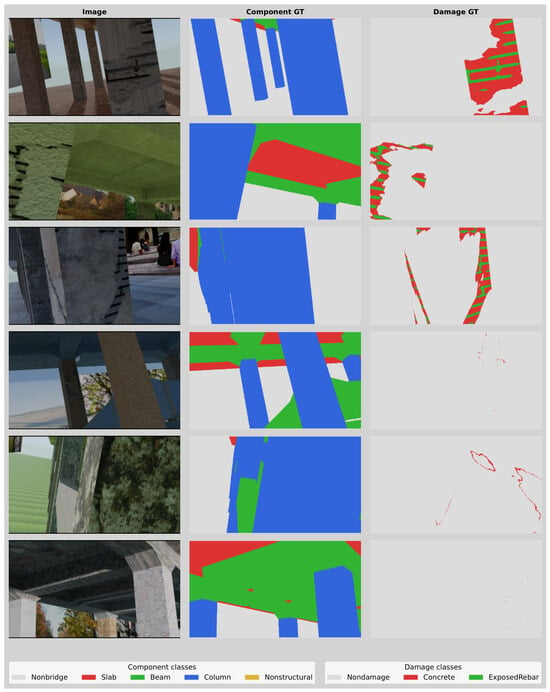
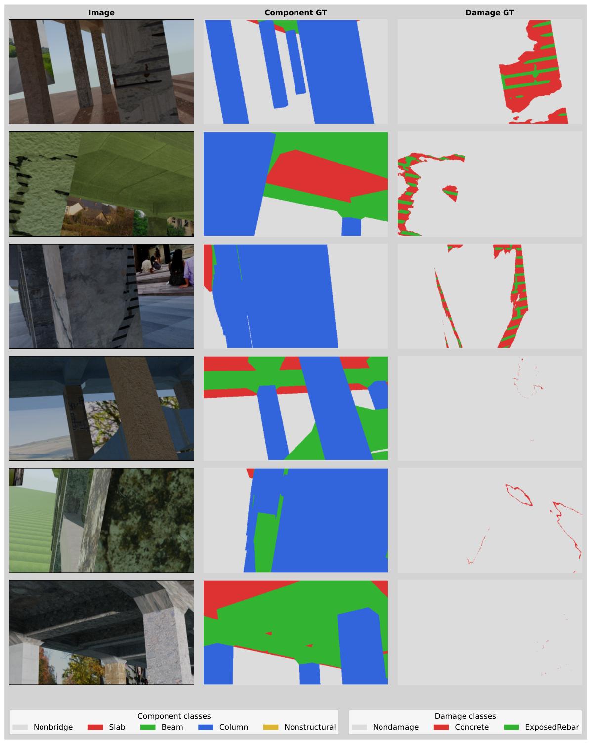
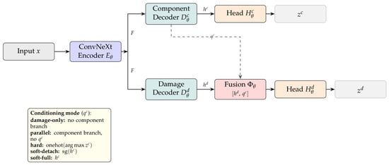
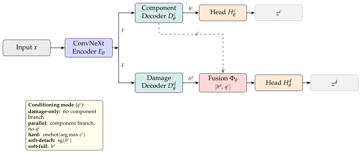
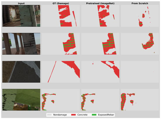
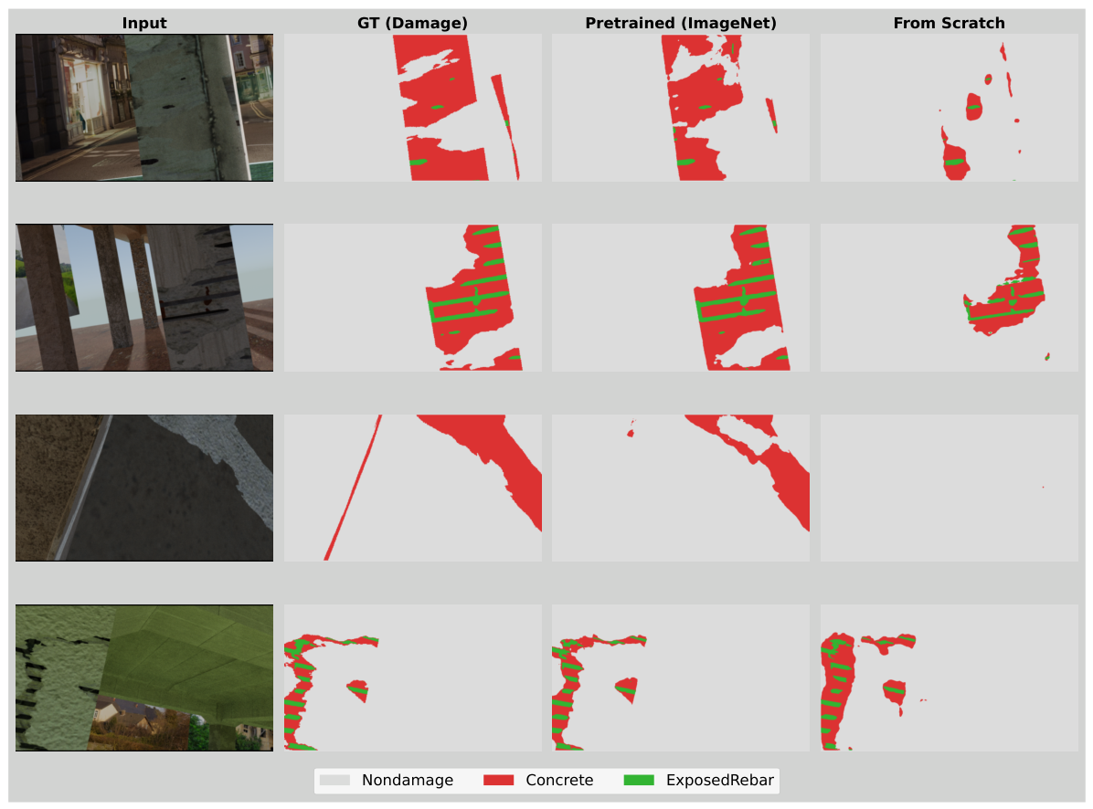
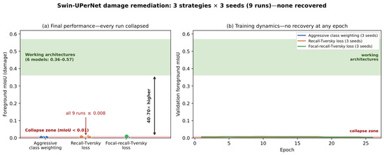
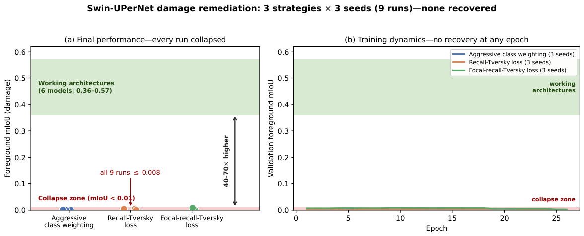
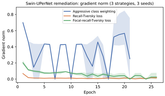
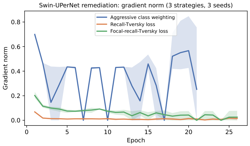
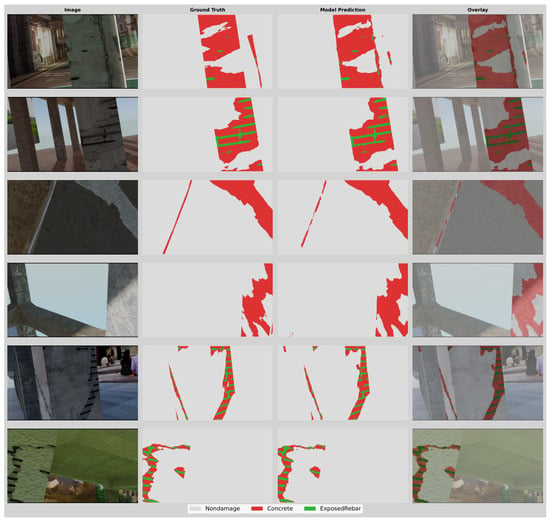
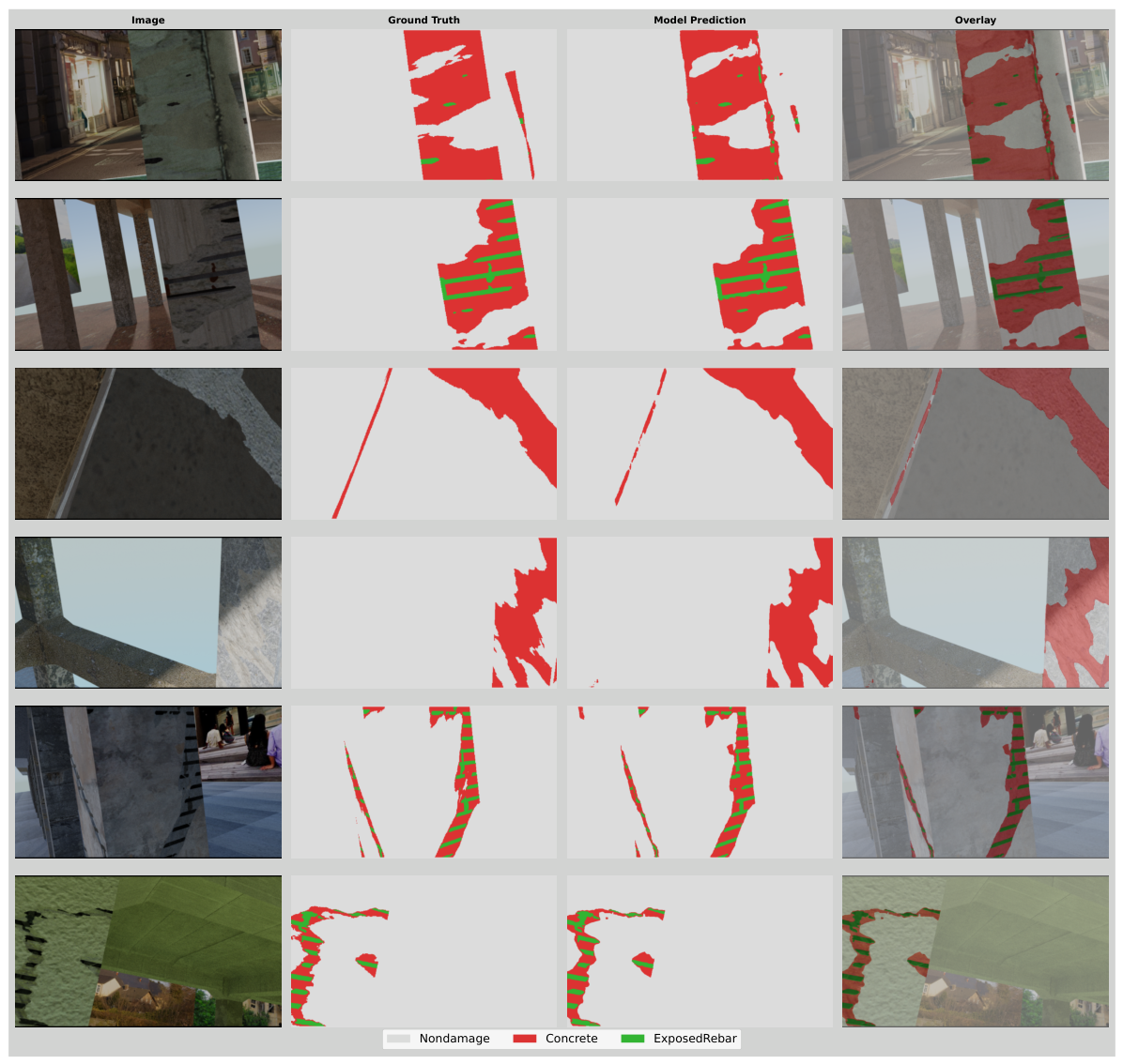
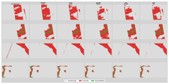
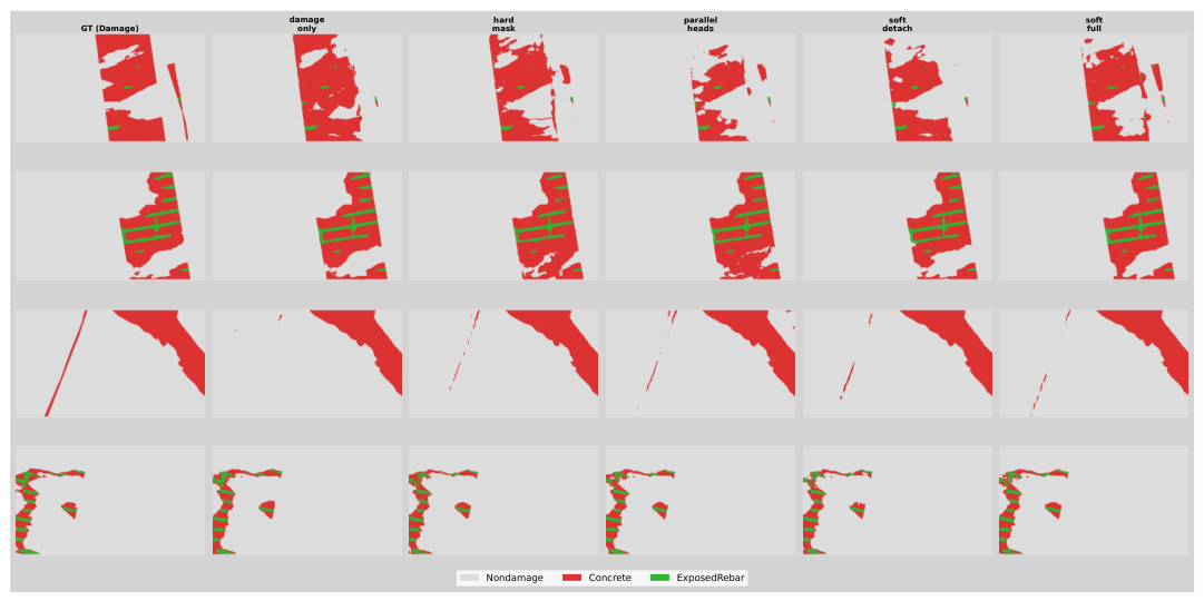
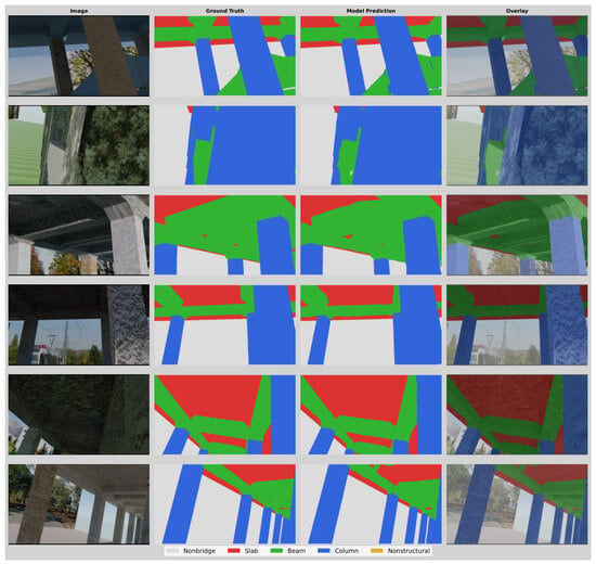
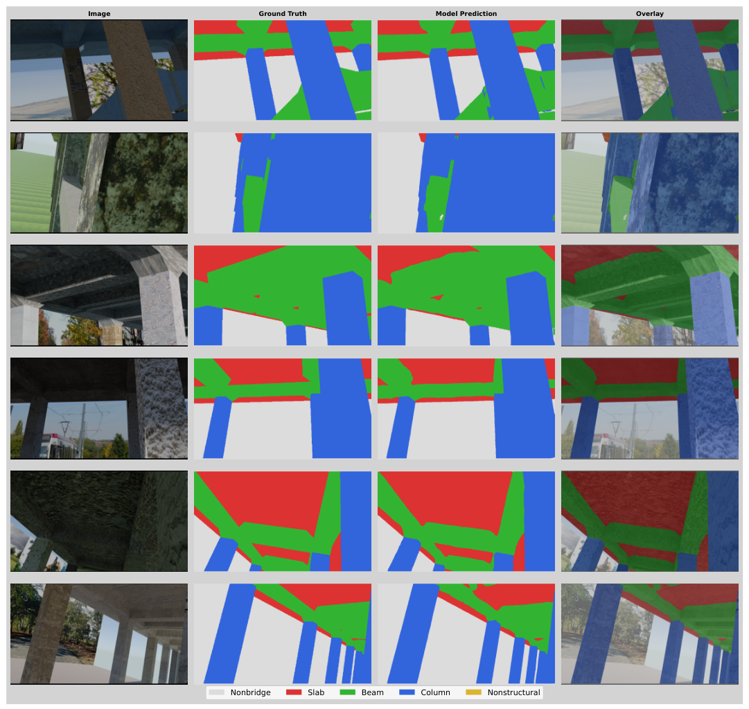
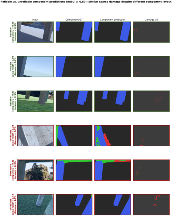
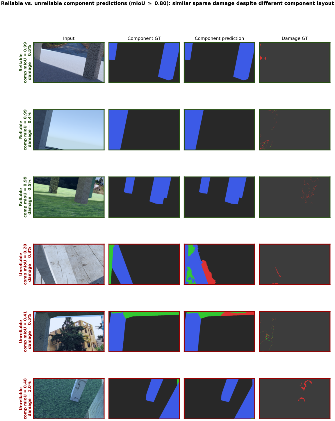
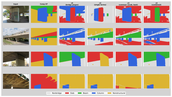
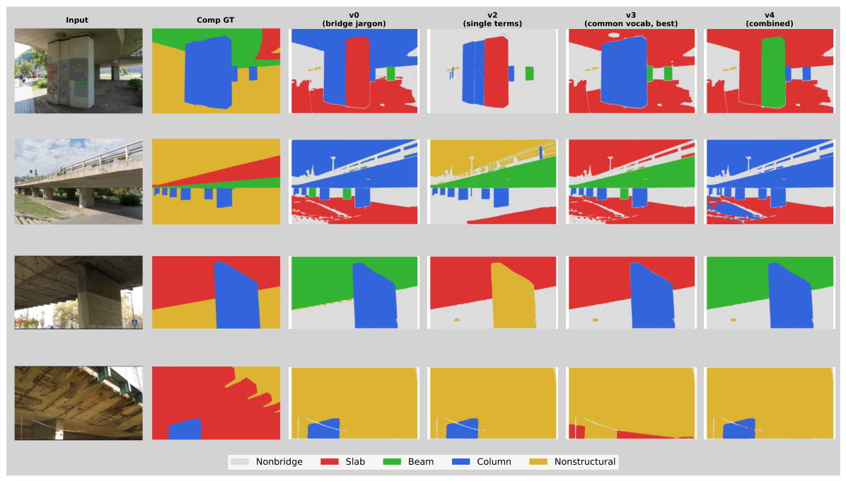
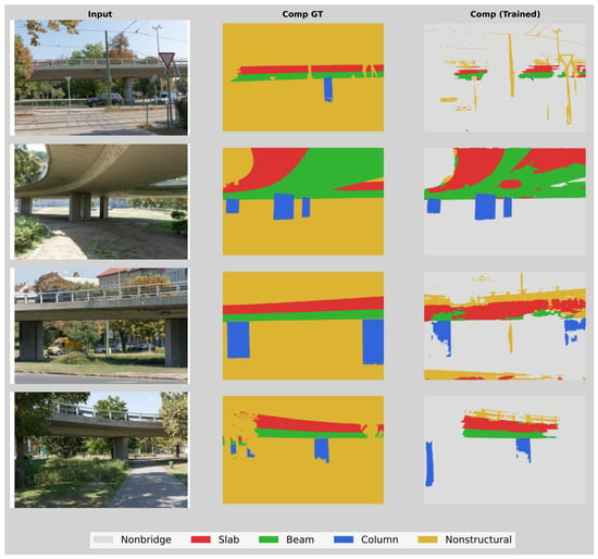
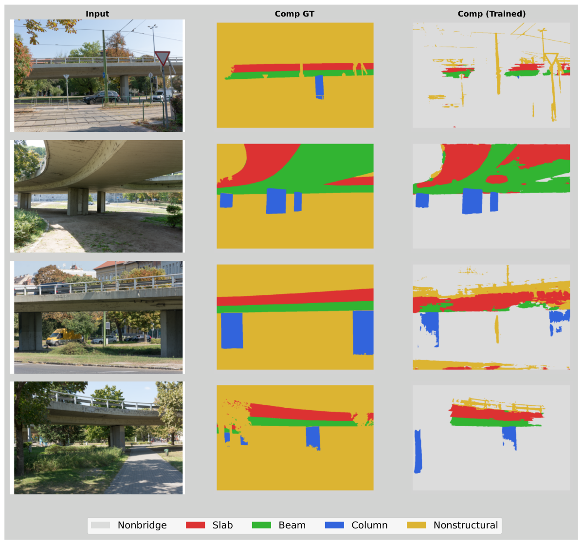

Disclaimer/Publisher’s Note: The statements, opinions and data contained in all publications are solely those of the individual author(s) and contributor(s) and not of MDPI and/or the editor(s). MDPI and/or the editor(s) disclaim responsibility for any injury to people or property resulting from any ideas, methods, instructions or products referred to in the content. |
© 2026 by the authors. Licensee MDPI, Basel, Switzerland. This article is an open access article distributed under the terms and conditions of the Creative Commons Attribution (CC BY) license.