


Abstract
Acute Lymphoblastic Leukemia (ALL) is a rapidly progressing blood cancer that demands timely and accurate diagnosis, particularly in pediatric patients. Conventional diagnosis relies on manual examination of peripheral blood smear images by hematologists, which is time-consuming, subjective, and prone to error. Although deep learning approaches have demonstrated high accuracy in medical imaging, many existing models are computationally intensive, limiting their use in resource-constrained clinical settings. To address these challenges, we propose LeukSNN, a lightweight spiking neural network (SNN) for automated ALL detection from peripheral blood smear images. Unlike conventional CNNs, SNNs employ sparse event-driven computations that can substantially reduce computational and energy requirements, making them attractive for deployment in low-resource healthcare environments. The proposed architecture combines depthwise separable convolutions, residual connections, and attention mechanisms within an SNN framework to achieve high classification performance with reduced computational cost. Experiments on three publicly available datasets demonstrate accuracies of 99.91–100%, while requiring only 8% and 28% of the multiplication and addition operations, respectively, of current state-of-the-art efficient methods. These results demonstrate that LeukSNN can achieve highly accurate and computationally efficient ALL classification on benchmark datasets, highlighting the potential of SNN-based approaches for future investigation in resource-constrained healthcare environments.
1. Introduction
Acute lymphoblastic leukemia (ALL) is the most prevalent form of cancer in children [1]. It is the result of an overproduction of immature lymphoid cells in bone marrow, which can enter the bloodstream and other organs. Early and accurate diagnosis is essential for initiating timely treatment and improving patient outcomes. Traditionally, diagnosis involves manual examination of stained peripheral blood smear (PBS) images by expert hematologists. This process, while effective, is labor-intensive, time-consuming, and susceptible to inter-observer variability. With the exponential growth of advances in artificial intelligence (AI), automated systems based on deep learning have emerged as powerful tools for enhancing the accuracy, speed, and objectivity of diagnostic workflows in hematopathology.
Among the various deep learning techniques, Artificial Neural Networks (ANNs), and in particular Convolutional Neural Networks (CNNs), have demonstrated remarkable success in the field of medical image analysis, due to their ability to learn hierarchical feature representations directly from pixel-level data. They have been widely applied across diverse diagnostic imaging tasks, including the segmentation of dermatological conditions [2], brain tumor classification [3], breast cancer detection [4], sickle cell anemia segmentation [5], and blood cell classification [6]. In recent years, CNNs have gained significant attention in hematology for the classification of ALL and its subtypes, with several recent studies reporting high accuracy across multiple benchmark datasets [7,8,9,10].
One of the key components that has allowed existing ALL classification networks to achieve their high accuracy results is the residual connection. Originally introduced for computer vision applications in He et al. [11], residual connections facilitate more effective training by allowing information to propagate across layers. This is accomplished by using identity mappings that add earlier inputs to the feature representations generated in deeper layers. This design not only mitigates optimization challenges in deep networks but also enhances representational capacity. Consequently, residual connections have been widely integrated into a range of image classification models [12,13,14], consistently demonstrating their effectiveness.
Although current CNN-based models for ALL detection achieve high diagnostic accuracy, they typically rely on large and complex architectures that demand significant computational resources. In particular, the extensive floating-point multiplications required by these networks result in substantial computational overhead, which can hinder real-time deployment and limit their practicality in resource-constrained clinical environments, such as smaller hospitals. One widely adopted strategy to mitigate this issue is the replacement of standard convolutions with depthwise separable convolutions [15]. The depthwise separable convolution substantially reduces the computational burden of a network while maintaining competitive accuracy. Its efficiency arises from decomposing the convolution into two sequential stages: a depthwise convolution, which applies spatial filtering independently to each channel, followed by a pointwise convolution, which integrates information across channels while preserving spatial structure. Requiring fewer multiplication operations, this two-step process has been demonstrated to provide a robust and computationally efficient alternative to the conventional convolution [16,17].
Another proposed solution to mitigate the high computational requirements of CNNs is the Spiking Neural Network (SNN) [18]. SNNs incorporate special spiking layers that propagate information through a network using binary values (0’s and 1’s). Unlike CNNs, which extract features through continuous-valued activations, SNNs encode and process information using discrete spike events distributed across time. Consequently, feature representations in SNNs are formed through temporal spike activity, allowing inactive neurons to remain silent and reducing the number of arithmetic operations performed during inference. The spikes (1’s) created in an SNN are generated according to membrane potential equations designed to approximate the behavior of biological neurons. These equations can be formulated to replicate a wide variety of biological processes, depending on the requirements of the network, with the Integrate-and-Fire (IF) and Leaky Integrate-and-Fire (LIF) neurons [19] being among the most commonly employed models. These models are designed to replicate simple neuro-biological dynamics, and are primarily used for their computational efficiency, though several other variations, including Adaptive Leaky Integrate and Fire (ALIF) [20] and Leaky Integrate and Fire or Burst (LIFB) [21] models have also been successfully deployed in deep SNNs. By disseminating information in a binary manner, SNNs are able to greatly reduce the number of multiplication operations they perform, thereby improving computational efficiency. SNNs have been the subject of several recent studies on medical data, including research on detecting skin cancer [22], breast cancer [23,24], lung disease [25], and liver tumors [26], and have shown promising results.
Despite their computational efficiency, the widespread use of SNNs has been hindered by their reduced accuracy. Many different solutions have been proposed to help SNNs better rival their ANN counterparts, and one that has been shown to work particularly well is the attention mechanism. Inspired by the human visual system’s ability to focus selectively on important regions of a scene [27,28], attention mechanisms help neural networks prioritize features that contain the most valuable information. Among these variations, the channel-wise Squeeze and Excite (SE) method [29] is one of the most widely used. Combining global average pooling, a small multi-layer perceptron, and a sigmoid function allows this mechanism to successfully increase a network’s task-specific performance, while adding minimal computational overhead. Another attention mechanism frequently employed in CNNs is the Convolutional Block Attention Module (CBAM) [30], which integrates an SE-like channel attention mechanism with spatial attention. The spatial attention component leverages global max-pooling and average-pooling operations, followed by a convolution and sigmoid function, to capture informative spatial features. By combining channel and spatial attention, CBAM is able to further enhance network performance, while still maintaining a relatively low additional computational cost. By incorporating different variations of these two attention mechanisms into SNN models, researchers have begun to bridge the accuracy gap between ANNs and SNNs [31,32,33,34].
Depthwise separable convolutions provide an effective means of reducing the computational overhead of CNNs by decreasing the number of parameters and convolutional operations required. Furthermore, SNNs offer improved computational efficiency through sparse, event-driven spike-based processing, which can substantially reduce computational and energy requirements. The complementary nature of these approaches makes their combination particularly well-suited for developing lightweight diagnostic models for resource-constrained clinical settings. Motivated by these advantages, we propose LeukSNN, a lightweight SNN-based framework for automated ALL detection from peripheral blood smear (PBS) imagery. The proposed architecture integrates depthwise separable convolutions, attention mechanisms, and residual connections within an SNN framework to achieve high classification performance while significantly reducing computational cost. Our proposed model is evaluated on the Acute Lymphoblastic Leukemia Image Dataset, ALL-IDB1, and ALL-IDB2 datasets to demonstrate its effectiveness. The contributions of this work are as follows:
- Our proposed LeukSNN achieves classification accuracies of 99.91%, 100%, and 100% on the Acute Lymphoblastic Leukemia Image Dataset, the ALL-IDB1 dataset, and the ALL-IDB2 dataset, respectively. Notably, this performance is attained while requiring approximately 8% of the multiplication operations and 28% of the addition operations compared to the current, most efficient, state-of-the-art methods.
- The proposed LeukSNN introduces a novel depthwise separable convolution and attention mechanism configuration for improving classification performance.
- The proposed SNN is, to the authors’ knowledge, the first designed for ALL classification.
- The proposed LeukSNN model is compared to other state-of-the-art methods to demonstrate its effectiveness.
2. Literature Review
In this section, we review past literature relating to our work, including research on Deep Learning for ALL detection and the use of SNNs for medical image classification.
2.1. Deep Learning for ALL Detection
In recent years, numerous deep learning approaches have been proposed for the automated detection and classification of ALL, with a strong emphasis on improving diagnostic accuracy, robustness, and computational efficiency. These methods can be broadly categorized into transfer learning-based approaches, hybrid feature extraction frameworks, attention-enhanced models, and lightweight architectures.
Early work by Genovese et al. [7] introduced cross-dataset transfer learning for ALL detection, demonstrating that both ResNet18 and Vision Transformer (ViT) architectures can generalize effectively across datasets while achieving state-of-the-art performance. In a subsequent study, Genovese et al. [35] further extended this work by incorporating explainable artificial intelligence techniques, enabling improved model transparency and interpretability while maintaining strong classification performance. Similarly, Perveen et al. [8] developed a clinically oriented web-based platform based on a ResNet152 backbone, enabling automated classification of ALL and its subtypes. Das et al. [36] further explored transfer learning by introducing an orthogonal softmax layer to enhance feature discrimination, resulting in improved classification performance for ALL detection tasks.
Several studies have explored hybrid architectures to improve feature representation. For instance, Islam et al. [37] fused features from DenseNet121 and VGG16 by processing segmented and raw PBS images separately, achieving high classification accuracy through complementary feature learning. Likewise, Omneya Attallah [10] combined CNN-based features with wavelet pooling, handcrafted descriptors, ReliefF feature selection, and SVM classification, achieving perfect accuracy on two ALL datasets. Mehan [38] further explored hybridization by integrating SqueezeNet with multiple machine learning classifiers, demonstrating improved diagnostic performance through ensemble decision-making. Das et al. [39] also proposed a hybrid lightweight framework combining MobileNetV2 and ShuffleNet to balance classification performance with computational efficiency. Finally, Jawahar et al. [40] introduced ALNett, a cluster layer-based deep convolutional neural network that enhances feature separability for ALL classification, demonstrating strong performance across benchmark datasets.
More recent works have focused on enhancing feature learning through attention mechanisms and advanced architectural designs. Masoudi et al. [41] introduced a variable-kernel channel-spatial attention (VKCS) module to refine region-specific features, significantly improving classification robustness. Similarly, Raghaw et al. [9] proposed CoTCoNet, a coupled Transformer–CNN architecture that jointly captures global and local features, followed by graph-based feature reconstruction and dual-stage optimization. Their network demonstrated its effectiveness by achieving state-of-the-art results across multiple datasets. Expanding on the use of attention, Baydilli [42] proposed an unsupervised, attention-guided, domain adaptation framework. Their proposed method improved generalization across datasets by aligning feature distributions while leveraging attention mechanisms to focus on diagnostically relevant regions.
Lightweight and efficient models have recently gained increased attention due to their suitability for real-world deployment. Ali et al. [43] proposed FDP-Net, which incorporates depthwise–pointwise feature fusion and dynamic pooling to achieve high accuracy with reduced computational complexity. Similarly, Batool and Byun [44] developed a lightweight EfficientNetB3-based model utilizing depthwise separable convolutions, achieving improved classification performance while maintaining computational efficiency. Finally, Hita et al. [45] further investigated uncertainty-aware models by integrating Bayesian convolutions and Monte Carlo dropout into pre-trained networks, improving reliability in ALL classification tasks.
2.2. SNNs for Medical Data Classification
Research demonstrating the effectiveness of SNNs for analyzing medical data has been the topic of several recent studies. Their low computational cost, combined with their ability to achieve high accuracies, has made them an appealing alternative to conventional ANNs, particularly in applications requiring efficient and real-time analysis. Existing approaches can be broadly categorized into spiking convolutional frameworks, hybrid CNN–SNN models, and attention-enhanced or sequence-aware architectures.
Several studies have explored the use of spiking convolutional neural networks (SCNNs) for medical image classification. Rajagopal et al. [25] proposed a custom SCNN for chest X-ray classification, incorporating soft leaky integrate-and-fire (SLIF) neurons with learnable parameters and an arithmetic optimization algorithm for parameter tuning. This combination enabled the model to achieve state-of-the-art performance across multiple lung disease classification tasks. Similarly, Senthil et al. [24] integrated SLIF neurons and a convolutional neural network for classifying breast cancer from mammogram imagery. Their method, including fast discrete curvature transforms and several other preprocessing steps, obtained superior accuracies while reducing computational time when compared to existing methods.
Hybrid CNN–SNN architectures have also been widely investigated to leverage the strengths of both paradigms. Kumar et al. [22] proposed the PCSN-Net system for detecting skin cancer from dermatological images. The system employs several preprocessing steps, including noise reduction, segmentation, and augmentation, before passing the images into the PCSN-Net model. The model fuses the outputs of a Parallel Convolutional Neural Network and an SNN to achieve superior results over existing models in terms of accuracy and inference time. Similarly, Tang et al. [23] combined a CNN with Nonlinear Spiking Neural P (NSNP) neurons to develop their proposed MSA-Net for breast cancer detection. The MSA-Net model incorporated a multistage attention mechanism into the CNN and integrated the biologically plausible autapse with the NSNP neurons. The result was a model capable of producing state-of-the-art accuracies.
More advanced architectures have focused on improving feature representation through attention mechanisms and architectural innovations. Ren et al. [26] proposed the LGMA-Net model. By combining depthwise separable convolutions with Spiking Neural P layers, the authors develop their proposed SNP convolutional transformer blocks and arranged them in a UNet-like architecture. Adding in their proposed Channel-Attentive Skip Connections (CASC) to help emphasize informative channel information, LGMA-Net achieved state-of-the-art results for both liver and tumor segmentation on several datasets. Bokhari et al. [46] designed three different spiking models for detecting several different diseases from pediatric chest x-ray images. The first model was a custom SCNN designed for spatial-temporal feature extraction. The second model, a Spiking Residual Network, incorporated residual connections within an SCNN to help better propagate information through the network. Finally, the third model combined an SCNN with spiking LSTM layers to create a Heuristic Spiking Neural Network (HSNN) that could capture fine-grained sequential correlations. All three models were evaluated using several accuracy metrics, with the HSNN model producing the highest accuracies across all disease categories.
Inspired by the use of SNNs for medical image classification and the need to create more efficient deep learning models for detecting ALL, we propose LeukSNN, one of the first SNNs for detecting ALL from PBS imagery. The proposed LeukSNN integrates channel and spatial attention with depthwise separable convolutions and residual connections to create an SNN alternative to existing deep learning models. Our LeukSNN architecture not only offers state-of-the-art levels of efficiency but also maintains the high classification accuracy expected from standard CNN models.
3. Materials and Methods
This section presents the architecture and implementation details of the proposed LeukSNN model. An overview of the complete network is shown in Figure 1a. The proposed architecture incorporates a novel Spiking Attention Depthwise Separable Convolution (SADS Conv) module for feature extraction. The following subsections describe the spiking neuron layers, the SADS Conv module, and the classification head, while details of the datasets, training procedures, and evaluation metrics are provided separately in the Experimental Setup subsection.
Figure 1.
Overview of the proposed LeukSNN architecture. The complete network architecture is shown in (a), where the input image is processed by five SADS Conv layers before reaching the final classification head. During inference, the input is propagated through the SADS Conv layers for T timesteps before being passed to the final classification head. The structure of the proposed SADS Conv layer is illustrated in (b). This layer combines depthwise separable convolutions with spatial attention, channel attention, spiking neurons, and residual connections to improve classification performance while maintaining computational efficiency.
3.1. Spiking Neuron Model
Many different spiking models have been proposed for use in spiking neural networks. In our work, we choose to use the Leaky Integrate-and-Fire (LIF) model due to its simplicity and proven effectiveness. The equations that define the LIF neurons in our network are as follows:
where is the membrane potential of the nth postsynaptic neuron at time step . The variable is the neuron’s decay constant, is the weight between the ith presynaptic neuron and the nth postsynaptic neuron, and is the output spike value from the ith presynaptic neuron. is the output spike value of the nth postsynaptic neuron, represents the Heaviside function, and is the membrane potential threshold of the postsynaptic neuron. In summary, Equation (1) represents the membrane potential update process of a neuron, Equation (2) is used to determine if a spike is generated, and Equation (3) resets the membrane potential of the neuron if a spike occurs.
In SNNs, the spiking output of the LIF layers is nondifferentiable, requiring the use of special methods to train the network. In our work, we make use of the surrogate gradient training method, which allows us to easily develop our proposed LeukSNN with existing deep learning libraries. The surrogate gradient function utilized by the LIF layers in our network is described in Fang et al. [47] and Eshraghian et al. [48], and is listed in Equation (4) below.
3.2. Spiking Attention Depthwise Separable Convolutions
The depthwise separable convolution, known for its efficiency, has had its effectiveness demonstrated in several different works, including MobileNet [16] and EfficientNet [17]. We find its efficiency well-suited for our proposed model and use it as the basis for the convolutions in our network. To further enhance the depthwise separable convolution’s efficiency and ability to detect spatial correlations, we propose a modified version that we refer to as the Spiking Attention DepthWise Separable Convolution (SADS Conv), due to its inclusion of attention mechanisms and spiking layers. While depthwise separable convolutions and attention mechanisms have been widely studied individually, their integration within SNNs for leukemia classification remains largely unexplored. The proposed SADS Conv extends the conventional depthwise separable convolution block by integrating spike-driven processing with channel attention, spatial attention, and a residual connection within a unified architecture. Furthermore, the placement of these components was specifically designed to maximize feature discrimination while preserving sparse neural activity, as demonstrated by the ablation studies presented in Section 5.1.
Depicted in Figure 1b, our SADS Conv layers begin with a depthwise convolution with a kernel size of 3, a stride of 2, and a padding of 1, followed by a batch normalization layer. After the batch normalization, we insert a CBAM [30] spatial attention mechanism. The spatial attention mechanism is inserted at this point to further enhance spatial correlations detected by the depthwise convolution. A diagram depicting our spatial attention mechanism can be seen in Figure 2a and is defined as follows.
Figure 2.
Overview of the attention mechanisms employed in LeukSNN. The spatial attention mechanism is shown in (a), while the channel attention mechanism is shown in (b). In the channel attention module, convolutional layers are used in place of the fully connected layers typically employed in the MLP component. For both attention mechanisms, convolutional kernel sizes are indicated in parentheses.
In Equations (5) and (6) above, is the spatial attention map and is the sigmoid function. The variable is a convolution with a kernel size of 7 × 7, a padding of 3, and an output channel size of 1. Finally, is a concatenation of global average pooling and global max pooling operations performed across the channel dimension of the input data , and is the spatially adjusted output data.
Following the spatial attention mechanism is an LIF layer and the pointwise convolution. The highest computational cost of a depthwise separable convolution typically comes from the pointwise convolution operation, as the expansion of the number of channels requires a large number of multiplication operations. To improve the efficiency of the depthwise separable convolution, we place an LIF layer between the spatial attention mechanism and the pointwise convolution. By placing an LIF layer before the pointwise convolution, as proposed in [49], it ensures the pointwise convolution performs only addition operations, greatly reducing its computational requirements. After the pointwise convolution is a batch normalization layer, followed by a channel attention mechanism. Our channel attention mechanism is based on the CBAM and Efficient Channel Attention (ECA) [50] methods, with the squeeze and excitation along the channel dimension done via two convolutions. The placement of the channel attention mechanism at this point aligns with the concept that the pointwise convolution is designed for detecting channel-wise correlations. An overview of the channel attention mechanism can be seen in Figure 2b, and its equations are as follows.
In Equations (7) and (8) above, is the channel attention map, represents the sigmoid function, and is the input data. is a global average pooling operation and is a global max pooling operation, both occurring in the spatial dimensions. The variables and are convolutional operations with 1 × 1 kernel sizes, and their output channel sizes are and , where C is the number of input channels, and r is a channel reduction factor. Finally, after multiplying the original input data by the channel attention map , the final output is produced. Once the channel attention has been applied, the processed features are combined with a residual pathway implemented using a 1 × 1 convolution before being passed through a final LIF layer. The final LIF layer helps to further reduce the computational requirements of the model by making it so that only spikes are passed to the next layer in the network.
3.3. Classification Head
In spiking neural networks, there are multiple ways to generate the final output of the network. While some methods choose to work with more biologically plausible output data in the form of spikes [51,52], others choose to reduce spiking values to floating-point values, making it easier to work with existing deep learning methods [32,33,34,49,53]. In this work, we choose to make use of the second technique, as it has been shown to produce the highest accuracies, with little cost to the network’s efficiency. For our final classification head, we make use of the method used in Yao et al. [32] and Hu et al. [54], where the output of the last spiking layer in the network is passed through a spatial average pooling layer, a temporal average pooling layer, and finally into a fully connected layer for generating raw output classifications. A diagram depicting the classification head in our network can be seen in Figure 3, and its equation is listed below.
Figure 3.
Overview of the LeukSNN classification head. Binary input data undergoes spatial and temporal averaging, transforming it into floating-point feature representations, which are subsequently passed to the fully connected layer for final classification.
In Equation (9), is the output of the network, is a fully connected layer, is average pooling in the temporal dimension, is global average pooling in the spatial dimensions, and is the spiking output of the last SADS Conv layer.
3.4. Experimental Setup
The performance of the proposed LeukSNN is evaluated using the three benchmark datasets described below. The results reported below are the average outcomes of 5-fold cross-validation. For all datasets, the proposed LeukSNN was trained using the Adam optimizer with an initial learning rate of 0.001. The remaining hyperparameter settings are provided in Table 1. All experiments were performed with the PyTorch 2.4 library using an NVIDIA RTX 4060 GPU and AMD Ryzen7 7735HS processor.
Table 1.
Detailed information pertaining to the hyperparameter settings of our network for each utilized dataset in our studies.
3.4.1. Datasets
To evaluate the effectiveness of our model, experiments are conducted on three datasets: ALL-IDB1 [55], ALL-IDB2 [55], and the Acute Lymphoblastic Leukemia image dataset (ALLID) [56]. Detailed information about each dataset is provided below, and example images are shown in Figure 4a–h. The datasets utilized in this study are publicly available benchmark datasets previously released for leukemia image analysis research, with no personally identifiable patient information contained within them. No direct patient recruitment or clinical data collection was performed by the authors. During training, the input images were augmented using the methods described in Table 2.
Figure 4.
Representative images from the evaluated datasets. Panels (a,b) show benign and malignant samples, respectively, from the ALL-IDB1 dataset. Panels (c,d) depict representative benign and malignant cell images from the ALL-IDB2 dataset. Panels (e–h) illustrate representative images from the ALLID corresponding to the benign, Early Pre-B, Pre-B, and Pro-B classes, respectively.
Table 2.
Data augmentation settings for each of the three datasets utilized in our studies.
To prevent data leakage, each dataset was first partitioned into five non-overlapping subsets for cross-validation using the KFold implementation from scikit-learn with shuffling enabled, after which data augmentation was applied exclusively to the training data within each fold. Consequently, validation samples remained completely unseen during training. As patient-level metadata was not available for the evaluated datasets, cross-validation partitioning was performed at the image level rather than the patient level. Although image-level overlap was prevented, the absence of patient identifiers may permit residual inter-sample similarity between folds, representing an inherent limitation of the currently available datasets. Consequently, the reported results should be interpreted as performance on benchmark datasets rather than as evidence of patient-independent clinical generalization. Information pertaining to the number of epochs, batch size, total timesteps, and learning rate scheduler used during training is provided with each dataset’s summary. For final classification, ALL-IDB1 and ALL-IDB2 were treated as binary tasks (benign versus malignant), while ALLID was treated as a four-class classification task consisting of the categories discussed below.
ALL-IDB1: This dataset contains 108 PBS images categorized as either benign or malignant, with each image containing one or more white blood cells. The images were collected by the Università degli Studi di Milano in September 2005 using magnification ranges of 300–500. The dataset was developed to support the evaluation of segmentation and classification algorithms for ALL diagnosis. After collection, each image was labeled by an expert oncologist to provide ground-truth annotations. For this dataset, the proposed model utilized 60 epochs for training with a batch size of 8. During our experiments, a binary cross-entropy loss function was employed in conjunction with a stepped learning rate scheduler, using a step size of 5 and a gamma of 0.5. The total number of timesteps the network employs was set to three.
ALL-IDB2: Created for testing the performance of classification algorithms, the ALL-IDB2 dataset was generated by cropping areas around individual cells in ALL-IDB1 images. The result is a dataset containing 130 benign and 130 malignant single white blood cell images. For the ALL-IDB2 dataset, the proposed model utilized 60 epochs for training with a batch size of 4. The total number of timesteps the network employed was set to four. A binary cross-entropy loss function was used for training in conjunction with a stepped learning rate scheduler using a step size of 5 and a gamma of 0.5.
Acute Lymphoblastic Leukemia Image Dataset (ALLID): Collected using a Zeiss camera and microscope with 100× magnification by the Taleqani Hospital (Tehran, Iran), the dataset consists of 3256 PBS images. The images are categorized into four subcategories: benign, early Pre-B (malignant), Pre-B (malignant), and Post-B (malignant). All images were subsequently labeled by an expert oncologist after collection. For our experiments on the ALLID, the proposed model utilized 100 epochs for training with a batch size of 16. The total number of timesteps employed by the network was set to 3, and a reduce on plateau learning rate scheduler with a reduction factor of 0.5, a patience setting of 3, and a minimum learning rate of 1 × 10⁻⁵ was used.
3.4.2. Evaluation Metrics
Classification Performance Metrics
In order to thoroughly assess our network’s performance, we employ accuracy (Equation (10)), precision (Equation (11)), recall (Equation (12)), and F1-score (Equation (13)) as evaluation metrics, each of which is described below. While accuracy can be used to determine the overall performance of a network, it is typically considered insufficient as the sole metric for medical applications. Medical datasets frequently contain class imbalances, which can produce inflated accuracies that do not reflect a model’s performance on minority classes. Therefore, incorporating precision, recall, and F1-Score as separate metrics allows for a more comprehensive understanding of a network’s capabilities. In Equations (10)–(13) , and represent true positive, true negative, false positive, and false negative results.
- Accuracy describes the proportion of correctly classified samples to the total number of samples in the dataset.
- Precision measures the proportion of correctly predicted positive samples in relation to the total number of positives predicted for the entire dataset. It is used to help determine how reliable a positive prediction is.
- Recall represents the proportion of correctly identified positive samples among all actual positive samples in the dataset, and is an indicator of a model’s ability to correctly detect positive samples.
- F1-Score, defined as the harmonic mean of precision and recall, is used to measure how reliable positive predictions are and how well a network detects positive samples in the dataset.
Computational Complexity and Energy Efficiency Metrics
The efficiency of SNNs is a consequence of placing spiking layers before standard ANN layers in a network. By doing so, the subsequent ANN layer multiplies its weights by binary spike values (0 or 1), effectively reducing computationally expensive multiplication operations to simpler addition operations. To evaluate computational efficiency, three metrics are considered throughout this study: the total number of multiplication operations, the total number of addition operations, and the corresponding theoretical energy consumption. Because multiplication operations are substantially more energy-intensive than additions, operation counts provide a practical measure of computational complexity. The corresponding theoretical energy consumption, computed using a common hardware energy model, provides a consistent estimate of computational efficiency that facilitates fair comparison across different network architectures.
The total energy consumption is calculated by tabulating the number of multiplication and addition operations the network requires and weighting them by their respective energy costs. First, the total number of additions performed by an SNN is given by
where represents the total number of addition operations the SNN performs. The variable denotes the number of ANN layers that are preceded by spiking layers, the variable denotes the total number of timesteps used by the network, and represents the number of synaptic connections (i.e., weights) in the n-th ANN layer. The variable represents the average firing rate of the preceding spiking layer at timestep t, which acts as a gating mechanism for the execution of addition operations. The firing rate is computed independently at each timestep by dividing the total number of spikes generated by the layer by the total number of neurons (B × C × H × W), where B, C, H, and W denote the batch, channel, height, and width dimensions, respectively. This formula reflects the fact that each spike results in a single weight accumulation, while inactive synapses (0’s) incur no computational cost.
While spiking layers greatly reduce the number of multiplication operations a network must perform, it does not eliminate them entirely. Certain components of a network, such as batch normalization, attention mechanisms, and other ANN layers not preceded by a spiking layer, still require standard multiply and accumulate operations. The total number of multiplication operations performed by these components is given by
where L denotes the number of ANN layers not preceded by a spiking layer, and is the total number of multiplication operations performed by the l-th layer at each time step. Finally, the total energy required by the network can be calculated as
where represents the total energy, is the energy required to perform a single multiplication operation, and is the energy required to perform a single addition operation. The terms and represent the total number of multiplication and addition operations a network must perform. For all ANN baselines used for comparison in our studies, energy consumption is computed using the formula described in Equation (16), and each multiply–accumulate (MAC) operation is counted as one multiplication and one addition. To calculate the number of MAC operations performed by each ANN baseline, the ptflops [57] library was utilized. Where publicly available implementations existed, they were used directly for complexity estimation; otherwise, network architectures were reconstructed from the descriptions provided in the original publications. All baseline models were evaluated using the same input image dimensions as LeukSNN to ensure a fair comparison. For our experiments, all networks are assumed to be running on a 45 nm chip. In this scenario, the energy required for a single multiplication operation is 3.7 pJ, and 0.9 pJ is required for a single addition operation [58].
4. Results
The experimental results on the ALL-IDB1 dataset are summarized in the confusion matrix in Figure 5a. The proposed LeukSNN achieves a 100% accuracy, precision, recall, and F1-score on this dataset, and Table 3 shows a quantitative comparison with existing state-of-the-art methods. While LeukSNN attains the same classification accuracy as the CoTCoNet and EfficientNet-V2M + VKCS methods, it delivers substantial computational savings. Specifically, the CoTCoNet and EfficientNet-V2M + VKCS approaches require 72.67 and 128 times more multiplication operations and 10.9 and 19.2 times more addition operations, respectively, than the proposed model. The significant reduction in computational complexity translates directly to a significant reduction in energy requirements, with our proposed LeukSNN requiring 1/62 the energy of CoTCoNet and 1/147 the energy of EfficientNet-V2M + VKCS.
Figure 5.
Normalized confusion matrices for the ALL-IDB1 dataset (a), ALL-IDB2 dataset (b), and ALLID (c).
Table 3.
Classification results for the ALL-IDB1 dataset. The results corresponding to the proposed LeukSNN are highlighted in bold for ease of comparison. The number of multiplication operations (Mult.) and addition operations (Add.) are reported in billions, while theoretical energy consumption (E) is listed in millijoules (mJ).
The improved efficiency of our model can be primarily attributed to its spike-based propagation of information, which drastically reduces the number of multiplication operations it performs, and is further enhanced by the sparse firing of neurons across timesteps. Figure 6a illustrates the average proportion of neurons spiking in each LIF layer of LeukSNN when processing an image from the ALL-IDB1 dataset. By maintaining an average spiking rate of 25.59% across all timesteps and layers, LeukSNN further improves its efficiency, as the lower spiking rate directly reduces the number of required addition operations. When comparing efficiency with other state-of-the-art methods, the closest competitor is MobileNet-V2 + ShuffleNet, which requires 0.44 billion multiplications and 0.44 billion additions. This corresponds to approximately 22 times more multiplications and 6.29 times more additions than our LeukSNN, resulting in an energy consumption that is 17 times higher. In addition to its greater computational cost, the MobileNet-V2 + ShuffleNet method also yielded a lower accuracy (−0.93%), precision (−2%), and F1-Score (−1.01%) compared to our proposed approach. While perfect classification performance was achieved on this dataset, these results should be interpreted in the context of the relatively constrained size and variability of the dataset. However, the reported metrics were obtained using 5-fold cross-validation with non-overlapping image partitions, providing evidence that the proposed LeukSNN generalizes well within the scope of this benchmark dataset.
Figure 6.
Graphs showing the average number of spiking neurons in each LIF layer at each time step for the ALL-IDB1 dataset (a), ALL-IDB2 dataset (b), and ALLID (c).
The experimental results on the ALL-IDB2 dataset are presented in the confusion matrix in Figure 5b, and Table 4 provides a comparison with other state-of-the-art methods. Once again, our proposed LeukSNN achieves an accuracy, precision, recall, and F1-score of 100%, matching the performance of CoTCoNet and Wavelet Pooling + ReliefF. Similar to the findings on the ALL-IDB1 dataset, LeukSNN demonstrates substantial improvements in efficiency over these two networks. Specifically, the CoTCoNet method requires 109 times the number of multiplications, 24.22 times the number of additions, and 46.88 times the energy, while the Wavelet Pooling + ReliefF approach requires 204.5 times more multiplications, 45.44 times more additions, and 117.56 times the energy. Figure 6b illustrates the percentage of spiking neurons for the ALL-IDB2 dataset, with an average spiking rate of 26.48% across all timesteps and layers. When compared with other efficiency-oriented methods, our closest competitor is MobileNet-V2 + ShuffleNet. Although the MobileNet-V2 + ShuffleNet method outperforms several state-of-the-art approaches in terms of computational efficiency, it does not match LeukSNN in either performance or energy consumption. Our model requires 0.05 times the multiplications, 0.20 times the additions, and 0.08 times the energy of MobileNet-V2 + ShuffleNet, while simultaneously achieving improvements of 1.54% in accuracy, precision, recall, and F1-Score. While perfect classification performance was observed on this dataset, the relatively small size and potential lack of variability should be taken into consideration when interpreting these results. Nevertheless, the reported performance was consistently achieved under a 5-fold cross-validation protocol with non-overlapping image partitions, demonstrating the effectiveness of the proposed LeukSNN on this benchmark dataset.
Table 4.
Classification results for the ALL-IDB2 dataset. The results corresponding to the proposed LeukSNN are highlighted in bold for ease of comparison. The number of multiplication operations (Mult.) and addition operations (Add.) are reported in billions, while theoretical energy consumption (E) is listed in millijoules (mJ).
The results of testing on the ALLID are shown in the confusion matrix in Figure 5c, with a quantitative comparison to other state-of-the-art methods provided in Table 5. On this dataset, the proposed LeukSNN achieved an accuracy of 99.91%, a precision of 99.87%, a recall of 99.92%, and an F1-score of 99.89%. Analysis of the confusion matrix in Figure 5c indicates consistently strong classification performance across all four ALLID categories. Benign samples were classified correctly in all cases, achieving a class recall of 100%. The Early Pre-B, Pre-B, and Pro-B subtypes also exhibited high recall values of approximately 99.91%, 99.89%, and 99.89%, respectively. The few classification errors observed were limited to isolated misclassifications between Early Pre-B and Benign samples, Pre-B and Pro-B samples, and Pro-B and Benign samples, each occurring at a rate of approximately 0.1%. Figure 6c illustrates the percentage of spiking neurons for processing an image in this dataset during inference, indicating an average spiking rate of 26.42% across all timesteps and layers. This level of spiking activity results in the network requiring only 0.02 billion multiplications and 0.07 billion additions. As shown in Table 3, LeukSNN outperforms most other state-of-the-art approaches, though it falls slightly short of the results generated by Wavelet Pooling + ReliefF and FDP-Net, which achieve marginally higher accuracies (by 0.09%), precisions (by 0.13%), recalls (by 0.08%), and F1-scores (by 0.11%). This slight reduction in classification performance is likely attributable to the lightweight design of LeukSNN, which prioritizes computational efficiency through the use of depthwise separable convolutions and sparse spike-based processing. In contrast, LeukSNN provides substantial reductions in computational complexity. Compared with Wavelet Pooling + ReliefF, LeukSNN requires 4.06 billion fewer multiplications and 3.86 billion fewer additions, resulting in an estimated energy reduction of 18.69 mJ. Similarly, when compared to FDP-Net, LeukSNN demonstrates significant computational savings, reducing multiplication and addition operations by approximately 92% and 72%, respectively, which corresponds to an energy reduction of approximately 89.7% (1.04 mJ). These results indicate that LeukSNN achieves performance comparable to the best-performing methods while requiring substantially fewer computational resources.
Table 5.
Classification results for the ALLID. The results corresponding to the proposed LeukSNN are highlighted in bold for ease of comparison. The number of multiplication operations (Mult.) and addition operations (Add.) are reported in billions, while theoretical energy consumption (E) is listed in millijoules (mJ).
5. Discussion
Our proposed model consists of several interconnected components designed to improve the classification of ALL, while maintaining a low computational cost. To evaluate the contribution of each major architectural component and to assess the robustness of the proposed design, a series of ablation and sensitivity studies were conducted. First, we analyze the individual contributions of the attention and residual mechanisms, as well as several alternative configurations of these components, to determine their impact on classification performance. Next, we investigate the impact of varying the number of timesteps on both classification accuracy and computational complexity. We then examine the behavior of LeukSNN under several different batch size, training epoch, and learning rate scenarios. Additionally, we compare our proposed solution against several CNN-based variants, including a CNN incorporating depthwise separable convolutions and a CNN utilizing a non-spiking counterpart of the proposed SADS Conv architecture, in which the same depthwise separable convolution and attention configuration is retained while the spiking layers are removed. Finally, heatmaps are generated to improve model interpretability and to examine the spatial regions most influential to the network’s classification decisions. The results of these experiments are presented and discussed in the sections below.
5.1. Attention and Residual Connection Effects
5.1.1. Contribution of Attention and Residual Connections
To evaluate the contributions of the attention mechanisms and residual connections employed in our SADS Conv layers, we conducted ablation studies on the ALLID. The results of experiments, in which individual components are selectively removed, are presented in Table 6. When both components have been removed, the resulting architecture reduces to a Spiking Convolutional Network (SCNN), and is referred to as such from this point forward.
Table 6.
Ablation studies evaluating the effects of removing the attention mechanisms and residual connection on the ALLID. Multiplication operations (Mult.) and addition operations (Add.) are reported in billions, while theoretical energy consumption (E) is reported in millijoules (mJ).
Incorporating the proposed attention mechanism scheme into the SCNN leads to an increase in classification performance, with accuracy improving by 1.2% and corresponding gains in precision (1.11%), recall (1.51%), and F1-score (1.42%). The concurrent improvements in precision and recall indicate more reliable predictions, with false negatives benefiting most significantly. In addition, the stability of the model across folds improves considerably, as evidenced by a reduction in standard deviation from 4.05 to 1.08. From a computational perspective, the inclusion of attention introduces an additional 10 million multiplication operations, while the number of addition operations remains largely unchanged relative to the base SCNN. These additional multiplications result in an incremental energy increase of 0.03 mJ.
Introducing the residual connections into the network yields a considerable performance enhancement over the standard SCNN, with accuracy increasing by 2.49%. The variability across folds is also greatly reduced, as reflected by a decrease of 3.99 in the standard deviation. Similarly, increases in precision, recall, and F1-scores can be seen. The large increases in precision (2.61%) and recall (3.01%) indicate an overall more robust model, capable of reducing both the number of false positive and false negative predictions. In terms of computational overhead, the residual connections introduce minimal additional cost. The number of multiplication operations remains relatively unchanged, as spike-based signals are propagated between SADS Conv layers, causing the multiplications associated with residual connections to be replaced by addition operations. These extra additions account for the approximately 30 million extra addition operations the network with residual connections requires, and are directly responsible for the 0.03 mJ increase in required energy. Compared to the attention-enhanced SCNN, the residual connection variant achieves higher gains in accuracy (1.29%), precision (1.5%), recall (1.5%), and F1-score (1.51%). Overall, the residual connections contribute more to the classification performance of the network than attention mechanisms, while incurring little to no extra computational cost, as both networks consume the same amount of energy (0.09 mJ).
The combination of the residual connection and attention mechanisms form the SADS Conv layers used throughout our LeukSNN. Relative to the base SCNN, LeukSNN shows increases in accuracy (2.68%), precision (2.8%), recall (3.27%), and F1-score (3.15%). These gains reflect a substantial improvement in classification capability, with false negatives decreasing most significantly, while false positives are also notably reduced. Consistent with earlier observations, LeukSNN exhibits increased stability across folds, achieving a much lower standard deviation score of 0.08. Although the base SCNN remains the most energy-efficient architecture, requiring approximately half the energy of the proposed model, this efficiency comes at the cost of significantly lower classification performance.
When compared to the SCNN augmented with attention, we see that LeukSNN outperforms it across all accuracy metric categories, with increases in accuracy (1.48%), precision (1.69%), recall (1.76%), and F1-Score (1.73%). Furthermore, LeukSNN demonstrates more stability across folds, as indicated by a reduction in standard deviation of 1.00. However, the attention-only SCNN remains more efficient in terms of computational cost, requiring fewer addition operations and achieving an energy savings of 0.03 mJ. Compared to the SCNN incorporating only residual connections, we see smaller but consistent improvements in accuracy (0.19%), precision (0.19%), recall (0.26%), and F1-score (0.22%). While the combination of attention and residual connections improves all metrics relatively uniformly, it has the greatest impact on reducing false negative predictions. From a computational standpoint, the residual-only SCNN remains more efficient, requiring 0.01 billion fewer multiplication operations and consequently consuming 0.03 mJ less energy than the proposed model.
Overall, both attention mechanisms and residual connections substantially improve the classification performance of the base SCNN. Although residual connections provide the largest individual performance gains, their combination with attention in our proposed SADS Conv layers enables LeukSNN to achieve peak classification accuracy, while introducing only minimal additional computational overhead.
5.1.2. Analysis of Attention Placement and Configuration
In this study, we examine the results of experiments on the ALLID utilizing several different configurations of our proposed SADS Conv block. The variations consist of a different placement of the residual connection, flipping the attention mechanism order, using only spatial attention, using only channel attention, and replacing both channel and spatial attention with full CBAM attention modules. The results of these studies are presented in Table 7, and a depiction of each variation is presented in Figure 7.
Table 7.
Results of ablation studies utilizing different configurations of the proposed SADS Conv block. Multiplication operations (Mult.) and addition operations (Add.) are reported in billions, while theoretical energy consumption (E) is reported in millijoules (mJ).
Figure 7.
Variations of the proposed SADS Conv block evaluated in the ablation study. (a) Residual connection applied after the spatial attention module. (b) Channel attention applied after the depthwise convolution and spatial attention applied after the pointwise convolution. (c) Spatial-attention-only configuration. (d) Channel-attention-only configuration. (e) Replacement of the proposed attention arrangement with a full CBAM attention module. In all configurations, batch normalization is applied after both the depthwise and pointwise convolutions but is omitted from the diagrams for clarity. Orange-shaded regions indicate removed layers, while red-highlighted regions indicate added layers.
When the residual connection is placed after the spatial attention mechanism, as illustrated in Figure 7a, the model achieves an accuracy of 98.86%, representing the largest performance reduction among all evaluated variants. Similar reductions are observed in precision (98.68%), recall (98.62%), and F1-score (98.65%). These results indicate that the placement of the residual connection plays a critical role in preserving discriminative feature information within the proposed architecture. Although this configuration provides a marginal reduction in energy consumption (0.11 mJ compared to 0.12 mJ for the proposed model), the substantial decrease in classification performance suggests that the resulting efficiency gain is insufficient to justify the architectural modification.
In the flipped attention configuration shown in Figure 7b, channel attention is applied after the depthwise convolution, while spatial attention is applied after the pointwise convolution. This arrangement achieves an accuracy of 99.82%, which is slightly lower than that of the proposed LeukSNN architecture. Corresponding reductions are also observed in precision (99.77%), recall (99.79%), and F1-score (99.78%). The energy consumption is reduced to 0.11 mJ, partially due to a lower average spiking activity (22.30%). These results suggest that the ordering of the attention mechanisms influences the quality of the learned feature representations and contributes to the overall performance of the network.
The spatial-attention-only variant, depicted in Figure 7c, achieves an accuracy of 99.82%, with precision, recall, and F1-score values of 99.76%, 99.83%, and 99.80%, respectively. Removing the channel attention module reduces the computational complexity by approximately 0.01 billion multiplication operations and decreases the energy requirement to 0.11 mJ. Although the reduction in performance is relatively small, the results indicate that channel attention contributes additional discriminative information beyond that provided by spatial attention alone.
Similarly, the channel-attention-only configuration shown in Figure 7d achieves an accuracy of 99.85%, with corresponding precision, recall, and F1-score values of 99.78%, 99.86%, and 99.82%, respectively. This variant also exhibits a reduction of approximately 0.01 billion multiplication operations and achieves the lowest energy consumption among all evaluated models (0.10 mJ). Compared with the spatial-attention-only configuration, the slightly higher mean classification performance obtained using channel attention alone suggests that channel-wise feature recalibration may contribute more strongly to model performance than spatial attention within the proposed architecture. However, the observed difference is relatively small, indicating that both attention mechanisms provide meaningful contributions to feature refinement.
Finally, replacing the proposed attention arrangement with a conventional CBAM, as shown in Figure 7e, results in an accuracy of 99.88%, with precision, recall, and F1-score values of 99.85%, 99.86%, and 99.86%, respectively. While the classification performance remains comparable to that of LeukSNN, the energy consumption increases from 0.12 mJ to 0.15 mJ, corresponding to an increase of approximately 25%. This additional overhead arises because the CBAM variant applies both channel and spatial attention operations within each attention block, increasing the number of computations required during inference. Despite the additional computational cost, the CBAM variant does not improve classification performance, indicating that the proposed attention arrangement provides a more favorable trade-off between classification accuracy and energy efficiency.
Overall, the ablation study demonstrates that each architectural component contributes to the final performance of LeukSNN. The most significant degradation occurs when the residual connection is repositioned after the spatial attention module, highlighting the importance of residual feature preservation. Furthermore, comparison of the single-attention variants indicates that channel attention provides a slightly greater contribution to mean classification performance than spatial attention. However, neither mechanism alone achieves the performance of the proposed architecture. The highest mean accuracy and F1-score are obtained when both attention mechanisms are integrated, demonstrating that channel-wise and spatial feature refinement act in combination to improve classification performance. Finally, while the proposed attention arrangement and CBAM achieve comparable classification performance, the proposed design reduces energy consumption by approximately 20%, demonstrating a more favorable trade-off between recognition performance and computational efficiency.
5.2. Timestep Effects on Accuracy and Complexity
In spiking neural networks, the number of timesteps employed directly influences both representational capacity and computational complexity. To investigate this trade-off, we evaluated LeukSNN on the ALLID using different timestep values of T = 1, 2, 3, 4, and 6, and compared the results with our proposed three-timestep configuration. For timestep configurations yielding identical classification accuracy, no statistically significant differences were observed in precision, recall, or F1-score. Furthermore, improvements in accuracy were consistently accompanied by proportional improvements in precision, recall, and F1-score. Accordingly, only accuracy is reported in this section to avoid redundancy.
As shown in Table 8, reducing T impairs the network’s accuracy, but also decreases the complexity. When T is set to 1 and 2, the network’s accuracy is decreased by 0.08%. In contrast, the efficiency of the network improves with these lower timestep configurations. Specifically, the one timestep method requires 10 million fewer multiplications and 40 million fewer additions, resulting in a savings of 0.08 mJ of energy. Similarly, the two timestep configuration required 10 million fewer multiplications and 20 million fewer additions, resulting in an energy decrease of 0.04 mJ. When T is set to 3, the network achieves its highest classification accuracy, and no further performance improvements are observed for larger timestep values. Increasing T to 4 yields the same accuracy, while introducing an additional 20 million addition operations, resulting in a 0.04 mJ energy increase. Even when T is set to 6, the network shows no improvement in accuracy, while the energy demand doubles.
Table 8.
Results of the ablation study evaluating the effects of varying the number of timesteps (T) used by LeukSNN on the ALLID. Multiplication operations (Mult.) and addition operations (Add.) are reported in billions, while theoretical energy consumption (E) is reported in millijoules (mJ).
As a result of the studies above, the three-timestep configuration was selected, as it consistently produced the highest accuracy, while incurring only a modest increase in computational complexity. This aligns with the opinion of the authors, where reliability for ALL detection is paramount due to the severity of the disease, and prioritizing the timestep configuration that yields maximum accuracy is preferable, even if it incurs slightly higher computational cost.
5.3. Batch Size, Training Epochs, and Learning Rate Effects on Classification Performance
In this section, we investigate the effects of varying the batch size, number of training epochs, and learning rate on the classification performance of the proposed LeukSNN for the ALLID. The energy consumption under these configurations is not included in this analysis, as no significant differences were observed across the selected parameter values.
As shown in Figure 8a, the batch size plays a critical role in determining the final classification performance of LeukSNN. For a batch size of 8, the model achieves a high average accuracy of 99.91%, accompanied by a moderate standard deviation (0.14). The corresponding precision (99.87%), recall (99.92%), and F1-score (99.89%) indicate strong and well-balanced classification performance. The selected batch size of 16 produces similarly strong results, maintaining an average accuracy of 99.91% but with a lower variance (std ≈ 0.08), suggesting slightly improved training stability. This configuration also achieves the highest F1-score (99.89%) among all tested batch sizes, along with consistently high precision and recall. When the batch size is increased to 32, a slight reduction in performance is observed. The average accuracy decreases to 99.88%, with a standard deviation of approximately 0.13. While the precision remains high (99.87%), both recall (99.84%) and F1-score (99.85%) show a marginal decline, indicating a minor loss in overall classification balance. In contrast, a larger batch size of 64 leads to a more noticeable degradation in performance. The average accuracy drops to 99.60%, and the variability increases substantially (std ≈ 0.49), indicating unstable convergence across folds. This setting also yields the lowest precision (99.56%), recall (99.50%), and F1-score (99.53%), further confirming reduced effectiveness. Overall, the results suggest that smaller batch sizes (8–16) provide the best accuracy and stability. Among these, the selected batch size of 16 emerges as the most favorable choice, offering consistently high performance with reduced variability, making it the preferred configuration for training the proposed LeukSNN.
Figure 8.
Results of sensitivity studies examining the effects of batch size (a), number of training epochs (b), and learning rates (c) on LeukSNN performance for the ALLID. Classification accuracy (red), precision (green), recall (blue), and F1-score (orange) are shown for all subfigures.
The impact of varying the number of training epochs is illustrated in Figure 8b. At 25 epochs, LeukSNN achieves an average accuracy of 99.72% with a low standard deviation (0.07), indicating stable but slightly under-optimized performance. The corresponding precision, recall, and F1-score (99.61%, 99.71%, and 99.66%, respectively) suggest that the model has not yet fully converged at this stage. Increasing the number of epochs to 50 results in a modest improvement, with the average accuracy rising to 99.78%. However, this setting exhibits a higher variance (std ≈ 0.14), indicating less consistent convergence across folds. The F1-score also improves to 99.74%, reflecting better overall classification balance. A more substantial gain is observed at the selected 100 epochs, where the model reaches an average accuracy of 99.91% with reduced variability (std ≈ 0.08). This configuration also achieves strong precision (99.87%), recall (99.92%), and F1-score (99.89%), indicating both high accuracy and stable convergence. Further increasing the training duration to 150 epochs does not yield meaningful improvements in accuracy, which remains effectively unchanged at 99.91%, with similar variance. While the F1-score (99.90%) is marginally higher than at 100 epochs, the difference is negligible, suggesting that the model has already reached convergence by 100 epochs. Overall, these results indicate that increasing the number of epochs improves the performance of our LeukSNN up to a point, after which gains plateau. An optimal balance is achieved at the selected value of 100 epochs, which provides near-maximum accuracy and stable performance without unnecessary additional training.
The results of the learning rate analysis are presented in Figure 8c. A value of 1 × 10⁻² achieved near-optimal performance, with an average accuracy of 99.88% and the lowest standard deviation (0.07), indicating both high accuracy and strong training stability. Decreasing the learning rate to 1 × 10⁻³ resulted in the highest overall accuracy (99.91%) and the best F1-score (99.89%), with slightly higher variability (std ≈ 0.08). In contrast, a high learning rate of 1 × 10⁻¹ led to a noticeable degradation in performance, with a lower average accuracy (98.65%) and significantly higher variance (std ≈ 0.78), indicating unstable training dynamics. At the lower end, a learning rate of 1 × 10⁻⁴ showed a slight decline in accuracy (99.78%) and increased variability (std ≈ 0.18) compared to 1 × 10⁻² and 1 × 10⁻³, suggesting that overly small learning rates may hinder effective convergence. Overall, these results indicate that learning rates in the range of 1 × 10⁻² to 1 × 10⁻³ provide the best trade-off between accuracy and stability in our LeukSNN, with 1 × 10⁻³ being selected for its slightly improved classification performance.
5.4. LeukSNN vs. CNNs
The proposed LeukSNN incorporates spiking layers in an effort to reduce the computational burden of the network. While the results shown so far demonstrate a substantial reduction in computational complexity compared to existing approaches, we further evaluate the benefits of spiking computation by comparing the proposed model with a standard CNN using depthwise separable convolutions (DS-CNN), as well as a CNN augmented with a non-spiking variant of the proposed SADS Conv architecture, in which the same depthwise separable convolution and attention configuration is preserved while the spiking layers are removed (LeukCNN). The goal of this study is to better understand the advantages of using spiking layers, and to assess the impact our attention and residual connection schema has on a non-spiking network. For clarity, both CNN models are also compared to the SCNN described in the Attention and Residual Connection Affects section.
As shown in Table 9, the DS-CNN exhibits substantially lower accuracy, precision, recall, and F1-score compared to all other models. Notably, it underperforms even the SCNN, despite the only architectural difference between the two models being the presence of spiking layers. The DS-CNN is particularly prone to false negative classifications, as reflected by its lower recall relative to precision. While the DS-CNN produces an overall lower accuracy than the SCNN, it does offer more consistent results across folds, as indicated by its standard deviation of only 1.11 compared to the 4.05 of the SCNN. However, its consistency remains inferior to that of the LeukCNN and LeukSNN models. In terms of complexity, the DS-CNN is more efficient than LeukCNN, requiring approximately half the number of multiplication and addition operations and consuming 0.48 times the energy. Nevertheless, it fails to outperform either the SCNN or LeukSNN in terms of efficiency, and its markedly lower classification performance renders it a less favorable solution overall.
Table 9.
Comparison of LeukSNN with the SCNN, DS-CNN, and LeukCNN variants on the ALLID. Multiplication operations (Mult.) and addition operations (Add.) are reported in billions, while theoretical energy consumption (E) is reported in millijoules (mJ).
Evaluating the capabilities of the LeukCNN model, we observe that its accuracy reaches the same level as the LeukSNN model, with precision, recall, and F1-Scores that are nearly identical as well. The variation seen across the folds is also comparable, although LeukSNN demonstrates slightly greater consistency, as evidenced by its lower standard deviation. Despite comparable performance, LeukSNN offers a more computationally efficient solution. Specifically, LeukSNN requires approximately one-third the number of multiplication operations while incurring only 1.16 times the number of addition operations compared to LeukCNN. As a result, LeukCNN consumes roughly 2.5 times more energy than LeukSNN, highlighting the efficiency advantages of spike-based computation.
Overall, these comparisons show that spiking layers enable substantial reductions in computational cost while preserving, and at times, improving classification performance relative to non-spiking CNNs. Although the proposed SADS Conv layers improved both architectures, their benefits are most pronounced when combined with spike-based computation, which allows for much lower computational overhead. This reinforces the suitability of our LeukSNN for efficient and reliable ALL classification.
5.5. Model Interpretability and Heatmap Visualization
While the proposed LeukSNN achieved high classification performance across all of the evaluated datasets, interpretability remains a critical consideration in medical diagnostic applications to ensure that the network focuses on clinically relevant image regions. To improve model transparency, heatmap visualizations are generated for the three datasets evaluated in this study using a modified Spike Activity Mapping (SAM) [62] approach. Drawing inspiration from the class-discriminative weighting strategies proposed in Grad-CAM [63] and SNN-crafted Grad-CAM [62], classifier-layer weights are integrated into the SAM aggregation process when deeper semantic feature maps are utilized. The equations defining the proposed method are provided below.
In Equation (17), denotes the spike activation at spatial location (x,y), channel c, and timestep t. For the ALLID and ALL-IDB1 datasets, which may contain multiple white blood cells and spatially heterogeneous image content, the final spike activation outputs from the fourth SADS Conv layer were used for heatmap generation. Selecting activations from this earlier layer preserves higher spatial resolution, enabling finer localization of discriminative cellular regions while mitigating excessive spatial generalization introduced during heatmap interpolation. For the ALL-IDB2 dataset, in which a single white blood cell is the predominant image feature, the spiking output values from the final SADS Conv layer in the network are used to generate heatmaps. Although the deeper feature maps used for this dataset exhibit lower spatial resolution, they retain sufficient structural detail after interpolation while providing stronger class-specific semantic representations.
For all datasets, spike activations are first aggregated temporally and subsequently squared prior to channel-wise summation. The squaring operation amplifies persistent, high-response neuronal activity while suppressing weak or spatially diffuse activations, thereby improving the localization of diagnostically relevant leukocyte regions. The channel weighting term , defined in Equation (18), was selected based on the semantic depth of the extracted feature maps. For the shallower fourth SADS Conv layer used in the ALLID and ALL-IDB1 datasets, uniform weighting () was sufficient, owing to the stronger preservation of spatial localization information at this depth. In contrast, the deeper final-layer activations employed for the ALL-IDB2 dataset benefited from class-discriminative weighting via the final classification layer weights . Applying to the squared activations suppresses negatively contributing semantic channels while emphasizing those with stronger positive contributions to the target class prediction, yielding a more precise localization of the features driving network classification decisions. Lastly, the aggregated activation map is normalized according to Equation (19) to generate the final heatmap representation. By scaling the values of M(x,y) to the interval [0,1], the normalization procedure enables consistent visual interpretation across different images, while the small constant ϵ = 1 × 10⁻⁸ ensures numerical stability when the minimum and maximum activation values are equal.
The resulting heatmaps for all three datasets are shown in Figure 9a–h. Across all datasets, stronger activations are consistently observed around white blood cell nuclei and surrounding morphological regions, while comparatively lower activations are present in background regions. Although residual background activations persist, this is partially attributable to the discrete spike-based encoding inherent to SNNs and the temporal accumulation of spike responses employed during visualization. Overall, the generated heatmaps demonstrate that LeukSNN learns clinically relevant spatial features rather than exploiting background artifacts, providing additional interpretability for the proposed model’s classification decisions.
Figure 9.
Heatmaps and corresponding input images for the three datasets evaluated in this study. Shown in (a–d) are Benign, Early Pre-B, Pre-B, and Pro-B samples, respectively, from the ALLID. Shown in (e,f) are Benign and Malignant samples from the ALL-IDB2 dataset and shown in (g,h) are Benign and Malignant samples from the ALL-IDB1 dataset.
6. Conclusions
Acute Lymphoblastic Leukemia is the most common form of leukemia found in children. Fast and accurate diagnosis is critical in order for treatments to be administered effectively. In this work, we have presented a novel SNN for Acute Lymphoblastic Leukemia detection. Our network, by utilizing attention and residual connections in combination with depthwise separable convolutions and spiking neurons, provides a computationally efficient alternative to existing deep learning models. By demonstrating state-of-the-art accuracy on three benchmark datasets, the proposed model highlights the potential of computationally efficient SNN-based approaches for future deployment in resource-constrained environments. Although the proposed model demonstrates substantial computational efficiency and high classification accuracy, several limitations remain. First, the relatively high spiking rate seen across all three datasets prevents the network from achieving the maximum efficiency offered by some SNN architectures. Second, the extent of this study is limited to three relatively small datasets, which may not fully capture all of the variability present in the white blood cells of each class. Furthermore, because patient-level metadata was unavailable for the evaluated datasets, cross-validation partitioning was performed at the image level rather than the patient level, which may permit residual similarity between training and validation folds. Finally, despite its strong performance, the proposed model does not reach the highest accuracy reported by existing methods. To address these limitations, future research should evaluate the proposed model on independent multi-center clinical datasets with patient-level metadata to establish patient-independent generalization performance and better assess clinical applicability. Additional studies may also investigate incorporating different attention variations, such as temporal or self-attention, to further improve classification performance, as well as approaches for reducing and improving neuron spike rates to further enhance computational efficiency. Nonetheless, we hope that the method proposed in this article helps inspire other researchers to investigate more efficient methods for medical-related tasks.
Author Contributions
K.T.: Conceptualization, Modelling, Analysis, Validation, Writing—original draft. W.T.: Analysis, Validation, Writing—review and editing. S.W.: Analysis, Validation, Supervision, Writing—review and editing. All authors have read and agreed to the published version of the manuscript.
Funding
This research received no external funding.
Data Availability Statement
The source code and implementation details, along with model configuration settings and training/cross-validation splits used in this study, will be made publicly available upon acceptance of this article. The datasets used in this study are publicly available from the following websites: ALL-IDB1 and ALL-IDB2: https://scotti.di.unimi.it/all/ (Accessed: 25 August 2025), ALLID: https://www.kaggle.com/datasets/mehradaria/leukemia (Accessed: 2 September 2025).
Acknowledgments
The authors thank the Artificial Intelligence Center (AIC) and MLIS Laboratory, College of Computing, Khon Kaen University, Thailand, for their support.
Conflicts of Interest
The authors declare no conflicts of interest.
References
- Lan, X.; Wu, J.; Liao, Z.; Wu, Y.; Hu, R. Prevalence of symptoms in children with acute lymphoblastic leukaemia: A systematic review and meta-analysis. BMC Cancer 2023, 23, 1113. [Google Scholar] [CrossRef] [Scilit] [PubMed]
- Liu, S.; Wang, P.; Lin, Y.; Zhou, B. IDSNet: Unifying local and global context for skin lesion image segmentation. Biomed. Signal Process. Control 2025, 108, 107961. [Google Scholar] [CrossRef] [Scilit]
- Wang, S.; Sun, K.; Wang, L.; Qu, L.; Yan, F.; Wang, Q.; Shen, D. Breast Tumor Segmentation in DCE-MRI with Tumor Sensitive Synthesis. IEEE Trans. Neural Netw. Learn. Syst. 2023, 34, 4990–5001. [Google Scholar] [CrossRef] [Scilit] [PubMed]
- Li, P.; Jin, Y.; Wang, M.; Liu, F. Sparse transformer and multipath decision tree: A novel approach for efficient brain tumor classification. Sci. Rep. 2025, 15, 28915. [Google Scholar] [CrossRef] [Scilit] [PubMed]
- Das, P.K.; Dash, A.; Meher, S. ACDSSNet: Atrous Convolution-Based Deep Semantic Segmentation Network for Efficient Detection of Sickle Cell Anemia. IEEE J. Biomed. Health Inform. 2024, 28, 5676–5684. [Google Scholar] [CrossRef] [Scilit] [PubMed]
- Zhu, H.; Zhu, Z.; Lu, S.-Y. BccT: An efficient transformer model for blood cell classification. Multimed. Syst. 2026, 32, 29. [Google Scholar] [CrossRef] [Scilit]
- Genovese, A.; Piuri, V.; Plataniotis, K.N.; Scotti, F. DL4ALL: Multi-Task Cross-Dataset Transfer Learning for Acute Lymphoblastic Leukemia Detection. IEEE Access 2023, 11, 65222–65237. [Google Scholar] [CrossRef] [Scilit]
- Perveen, S.; Alourani, A.; Shahbaz, M.; Ashraf, M.U.; Hamid, I. A Framework for Early Detection of Acute Lymphoblastic Leukemia and Its Subtypes from Peripheral Blood Smear Images Using Deep Ensemble Learning Technique. IEEE Access 2024, 12, 29252–29268. [Google Scholar] [CrossRef] [Scilit]
- Raghaw, C.S.; Sharma, A.; Bansal, S.; Rehman, M.Z.U.; Kumar, N. CoTCoNet: An optimized coupled transformer-convolutional network with an adaptive graph reconstruction for leukemia detection. Comput. Biol. Med. 2024, 179, 108821. [Google Scholar] [CrossRef] [Scilit] [PubMed]
- Attallah, O. Acute lymphocytic leukemia detection and subtype classification via extended wavelet pooling based-CNNs and statistical-texture features. Image Vis. Comput. 2024, 147, 105064. [Google Scholar] [CrossRef] [Scilit]
- He, K.; Zhang, X.; Ren, S.; Sun, J. Deep Residual Learning for Image Recognition. In 2016 IEEE Conference on Computer Vision and Pattern Recognition (CVPR); IEEE: Las Vegas, NV, USA, 2016; pp. 770–778. [Google Scholar] [CrossRef] [Scilit]
- Woo, S.; Debnath, S.; Hu, R.; Chen, X.; Liu, Z.; Kweon, I.S.; Xie, S. ConvNeXt V2: Co-designing and Scaling ConvNets with Masked Autoencoders. In 2023 IEEE/CVF Conference on Computer Vision and Pattern Recognition (CVPR); IEEE: Vancouver, BC, Canada, 2023; pp. 16133–16142. [Google Scholar] [CrossRef] [Scilit]
- Li, Y.; Wu, C.-Y.; Fan, H.; Mangalam, K.; Xiong, B.; Malik, J.; Feichtenhofer, C. MViTv2: Improved Multiscale Vision Transformers for Classification and Detection. In 2022 IEEE/CVF Conference on Computer Vision and Pattern Recognition (CVPR); IEEE: New Orleans, LA, USA, 2022; pp. 4794–4804. [Google Scholar] [CrossRef] [Scilit]
- Tan, M.; Le, Q.V. EfficientNetV2: Smaller Models and Faster Training. In 38th International Conference on Machine Learning; Proceedings of Machine Learning Research: Cambridge, MA, USA, 2021. [Google Scholar]
- Chollet, F. Xception: Deep Learning with Depthwise Separable Convolutions. In 2017 IEEE Conference on Computer Vision and Pattern Recognition (CVPR); IEEE: Honolulu, HI, USA, 2017; pp. 1800–1807. [Google Scholar] [CrossRef] [Scilit]
- Howard, A.G.; Zhu, M.; Chen, B.; Kalenichenko, D.; Wang, W.; Weyand, T.; Andreetto, M.; Adam, H. MobileNets: Efficient Convolutional Neural Networks for Mobile Vision Applications. arXiv 2017, arXiv:1704.04861. [Google Scholar] [CrossRef] [Scilit]
- Tan, M.; Le, Q.V. EfficientNet: Rethinking Model Scaling for Convolutional Neural Networks. arXiv 2020, arXiv:1905.11946. [Google Scholar] [CrossRef] [Scilit]
- Maass, W. Networks of spiking neurons: The third generation of neural network models. Neural Netw. 1997, 10, 1659–1671. [Google Scholar] [CrossRef] [Scilit]
- Abbott, L.F. Lapicque’s introduction of the integrate-and-fire model neuron (1907). Brain Res. Bull. 1999, 50, 303–304. [Google Scholar] [CrossRef] [Scilit] [PubMed]
- Liu, Q.; Cai, M.; Chen, K.; Ai, Q.; Ma, L. Reconstruction of Adaptive Leaky Integrate-and-Fire Neuron to Enhance the Spiking Neural Networks Performance by Establishing Complex Dynamics. IEEE Trans. Neural Netw. Learn. Syst. 2025, 36, 2619–2633. [Google Scholar] [CrossRef] [Scilit] [PubMed]
- Tian, Y.; Li, Y.; Chen, K.; Zhang, Z.; Tong, E.; Liu, J.; Qin, F.; Zheng, Z.; Niu, W. Towards Label-Efficient Deep Learning-Based Aging-Related Bug Prediction with Spiking Convolutional Neural Networks. IEEE Trans. Emerg. Top. Comput. 2025, 13, 314–329. [Google Scholar] [CrossRef] [Scilit]
- Kumar, K.A.; Vanmathi, C. A hybrid parallel convolutional spiking neural network for enhanced skin cancer detection. Sci. Rep. 2025, 15, 11137. [Google Scholar] [CrossRef] [Scilit] [PubMed]
- Tang, Y.; Yang, B.; Peng, H.; Luo, X. Multi-stages attention breast cancer classification based on nonlinear spiking neural P neurons with autapses. Eng. Appl. Artif. Intell. 2025, 142, 109869. [Google Scholar] [CrossRef] [Scilit]
- Senthil Prakash, T.; Kannan, G.; Prabhakaran, S.; Prajapati, B.P. Deep convolutional spiking neural network fostered automatic detection and classification of breast cancer from mammography images. Res. Biomed. Eng. 2023, 39, 833–841. [Google Scholar] [CrossRef] [Scilit]
- Rajagopal, R.; Karthick, R.; Meenalochini, P.; Kalaichelvi, T. Deep Convolutional Spiking Neural Network optimized with Arithmetic optimization algorithm for lung disease detection using chest X-ray images. Biomed. Signal Process. Control 2023, 79, 104197. [Google Scholar] [CrossRef] [Scilit]
- Ren, W.; Li, B.; Peng, H.; Wang, J. Lgma-net: Liver and tumor segmentation methods based on local–global feature mergence and attention mechanisms. Signal Image Video Process. 2025, 19, 43. [Google Scholar] [CrossRef] [Scilit]
- Saenz, M.; Buracas, G.T.; Boynton, G.M. Global effects of feature-based attention in human visual cortex. Nat. Neurosci. 2002, 5, 631–632. [Google Scholar] [CrossRef] [Scilit] [PubMed]
- Hollingworth, A.; Bahle, B. Feature-based guidance of attention by visual working memory is applied independently of remembered object location. Atten. Percept. Psychophys. 2020, 82, 98–108. [Google Scholar] [CrossRef] [Scilit] [PubMed]
- Hu, J.; Shen, L.; Sun, G. Squeeze-and-Excitation Networks. In 2018 IEEE/CVF Conference on Computer Vision and Pattern Recognition; IEEE: Salt Lake City, UT, USA, 2018; pp. 7132–7141. [Google Scholar] [CrossRef] [Scilit]
- Woo, S.; Park, J.; Lee, J.-Y.; Kweon, I.S. CBAM: Convolutional Block Attention Module. arXiv 2018, arXiv:1807.06521. [Google Scholar] [CrossRef] [Scilit]
- Yao, M.; Gao, H.; Zhao, G.; Wang, D.; Lin, Y.; Yang, Z.; Li, G. Temporal-wise Attention Spiking Neural Networks for Event Streams Classification. arXiv 2021, arXiv:2107.11711. [Google Scholar] [CrossRef] [Scilit]
- Yao, M.; Zhao, G.; Zhang, H.; Hu, Y.; Deng, L.; Tian, Y.; Xu, B.; Li, G. Attention Spiking Neural Networks. IEEE Trans. Pattern Anal. Mach. Intell. 2023, 45, 9393–9410. [Google Scholar] [CrossRef] [Scilit] [PubMed]
- Cai, W.; Sun, H.; Liu, R.; Cui, Y.; Wang, J.; Xia, Y.; Yao, D.; Guo, D. A Spatial–Channel–Temporal-Fused Attention for Spiking Neural Networks. IEEE Trans. Neural Netw. Learn. Syst. 2024, 35, 14315–14329. [Google Scholar] [CrossRef] [Scilit] [PubMed]
- Lian, S.; Shen, J.; Wang, Z.; Tang, H. IM-LIF: Improved Neuronal Dynamics with Attention Mechanism for Direct Training Deep Spiking Neural Network. IEEE Trans. Emerg. Top. Comput. Intell. 2024, 8, 2075–2085. [Google Scholar] [CrossRef] [Scilit]
- Genovese, A.; Piuri, V.; Scotti, F. A decision support system for acute lymphoblastic leukemia detection based on explainable artificial intelligence. Image Vis. Comput. 2024, 151, 105298. [Google Scholar] [CrossRef] [Scilit]
- Das, P.K.; Sahoo, B.; Meher, S. An Efficient Detection and Classification of Acute Leukemia Using Transfer Learning and Orthogonal Softmax Layer-Based Model. IEEE/ACM Trans. Comput. Biol. Bioinform. 2023, 20, 1817–1828. [Google Scholar] [CrossRef] [Scilit] [PubMed]
- Islam, M.M.; Rifat, H.R.; Shahid, M.S.B.; Akhter, A.; Uddin, M.A. Utilizing Deep Feature Fusion for Automatic Leukemia Classification: An Internet of Medical Things-Enabled Deep Learning Framework. Sensors 2024, 24, 4420. [Google Scholar] [CrossRef] [Scilit] [PubMed]
- Mehan, V. Artificial Intelligence Powered Automated and Early Diagnosis of Acute Lymphoblastic Leukemia Cancer in Histopathological Images: A Robust SqueezeNet-Enhanced Machine Learning Framework. Int. J. Telemed. Appl. 2025, 2025, 2257215. [Google Scholar] [CrossRef] [Scilit] [PubMed]
- Das, P.K.; Meher, S.; Rath, A.; Panda, G. An efficient deep learning system for automatic detection of Acute Lymphoblastic Leukemia. ISA Trans. 2025, 158, 488–496. [Google Scholar] [CrossRef] [Scilit] [PubMed]
- Jawahar, M.; H, S.; L, J.A.; Gandomi, A.H. ALNett: A cluster layer deep convolutional neural network for acute lymphoblastic leukemia classification. Comput. Biol. Med. 2022, 148, 105894. [Google Scholar] [CrossRef] [Scilit] [PubMed]
- Masoudi, B. VKCS: A pre-trained deep network with attention mechanism to diagnose acute lymphoblastic leukemia. Multimed. Tools Appl. 2023, 82, 18967–18983. [Google Scholar] [CrossRef] [Scilit]
- Baydilli, Y.Y. Unsupervised attention-guided domain adaptation model for Acute Lymphocytic Leukemia (ALL) diagnosis. Biomed. Signal Process. Control 2025, 101, 107159. [Google Scholar] [CrossRef] [Scilit]
- Ali, A.; Pal, R.; Paul, A.; Sarkar, R. FDP-Net: Fourier transform guided lightweight depthwise and pointwise dynamic pooling based neural network for medical image classification. Appl. Soft Comput. 2025, 184, 113824. [Google Scholar] [CrossRef] [Scilit]
- Batool, A.; Byun, Y.-C. Lightweight EfficientNetB3 Model Based on Depthwise Separable Convolutions for Enhancing Classification of Leukemia White Blood Cell Images. IEEE Access 2023, 11, 37203–37215. [Google Scholar] [CrossRef] [Scilit]
- Hita, X.; Javed, F.; Lodi, S. Reliable leukemia detection via transfer-enhanced Bayesian CNNs. Comput. Biol. Med. 2026, 202, 111419. [Google Scholar] [CrossRef] [Scilit] [PubMed]
- Bokhari, S.M.; Sohaib, S.; Shafi, M. Pediatric chest X-ray diagnosis using neuromorphic models. Comput. Biol. Med. 2025, 192, 110173. [Google Scholar] [CrossRef] [Scilit] [PubMed]
- Fang, W.; Yu, Z.; Chen, Y.; Masquelier, T.; Huang, T.; Tian, Y. Incorporating Learnable Membrane Time Constant to Enhance Learning of Spiking Neural Networks. In 2021 IEEE/CVF International Conference on Computer Vision (ICCV); IEEE: Montreal, QC, Canada, 2021; pp. 2641–2651. [Google Scholar] [CrossRef] [Scilit]
- Eshraghian, J.K.; Ward, M.; Neftci, E.O.; Wang, X.; Lenz, G.; Dwivedi, G.; Bennamoun, M.; Jeong, D.S.; Lu, W.D. Training Spiking Neural Networks Using Lessons from Deep Learning. Proc. IEEE 2023, 111, 1016–1054. [Google Scholar] [CrossRef] [Scilit]
- Yao, M.; Qiu, X.; Hu, T.; Hu, J.; Chou, Y.; Tian, K.; Liao, J.; Leng, L.; Xu, B.; Li, G. Scaling Spike-Driven Transformer with Efficient Spike Firing Approximation Training. IEEE Trans. Pattern Anal. Mach. Intell. 2025, 47, 2973–2990. [Google Scholar] [CrossRef] [Scilit] [PubMed]
- Wang, Q.; Wu, B.; Zhu, P.; Li, P.; Zuo, W.; Hu, Q. ECA-Net: Efficient Channel Attention for Deep Convolutional Neural Networks. In 2020 IEEE/CVF Conference on Computer Vision and Pattern Recognition (CVPR); IEEE: Seattle, WA, USA, 2020; pp. 11531–11539. [Google Scholar] [CrossRef] [Scilit]
- Mozafari, M.; Kheradpisheh, S.R.; Masquelier, T.; Nowzari-Dalini, A.; Ganjtabesh, M. First-Spike-Based Visual Categorization Using Reward-Modulated STDP. IEEE Trans. Neural Netw. Learn. Syst. 2018, 29, 6178–6190. [Google Scholar] [CrossRef] [Scilit] [PubMed]
- Liu, D.; Bellotto, N.; Yue, S. Deep Spiking Neural Network for Video-Based Disguise Face Recognition Based on Dynamic Facial Movements. IEEE Trans. Neural Netw. Learn. Syst. 2020, 31, 1843–1855. [Google Scholar] [CrossRef] [Scilit] [PubMed]
- Zhu, R.-J.; Zhang, M.; Zhao, Q.; Deng, H.; Duan, Y.; Deng, L.-J. TCJA-SNN: Temporal-Channel Joint Attention for Spiking Neural Networks. IEEE Trans. Neural Netw. Learn. Syst. 2025, 36, 5112–5125. [Google Scholar] [CrossRef] [Scilit] [PubMed]
- Hu, Y.; Deng, L.; Wu, Y.; Yao, M.; Li, G. Advancing Spiking Neural Networks towards Deep Residual Learning. arXiv 2023, arXiv:2112.08954. [Google Scholar] [CrossRef] [Scilit]
- Labati, R.D.; Piuri, V.; Scotti, F. All-IDB: The acute lymphoblastic leukemia image database for image processing. In 2011 18th IEEE International Conference on Image Processing; IEEE: Brussels, Belgium, 2011; pp. 2045–2048. [Google Scholar] [CrossRef] [Scilit]
- Aria, M.; Ghaderzadeh, M.; Bashash, D.; Abolghasemi, H.; Asadi, F.; Hosseini, A. Acute Lymphoblastic Leukemia (ALL) Image Dataset. Kaggle 2021. Available online: https://www.kaggle.com/datasets/mehradaria/leukemia (accessed on 15 July 2025). [CrossRef] [Scilit]
- Sovrasov, V. Ptflops: A Flops Counting Tool for Neural Networks in Pytorch Framework. 2018. Available online: https://github.com/sovrasov/flops-counter.pytorch (accessed on 25 August 2025).
- Horowitz, M. 1.1 Computing’s energy problem (and what we can do about it). In 2014 IEEE International Solid-State Circuits Conference Digest of Technical Papers (ISSCC); IEEE: San Francisco, CA, USA, 2014; pp. 10–14. [Google Scholar] [CrossRef] [Scilit]
- Mustaqim, T.; Fatichah, C.; Suciati, N.; Obi, T.; Lee, J.-S. Focusaugmix: A Data Augmentation Method for Enhancing Acute Lymphoblastic Leukemia Classification. Intell. Syst. Appl. 2025, 26, 200512. [Google Scholar] [CrossRef] [Scilit]
- Zhang, T.; Xue, G. Fuzzy attention-based deep neural networks for acute lymphoblastic leukemia diagnosis. Appl. Soft Comput. 2025, 171, 112810. [Google Scholar] [CrossRef] [Scilit]
- Thiriveedhi, A.; Ghanta, S.; Biswas, S.; Pradhan, A.K. ALL-Net: Integrating CNN and explainable-AI for enhanced diagnosis and interpretation of acute lymphoblastic leukemia. PeerJ Comput. Sci. 2025, 11, e2600. [Google Scholar] [CrossRef] [Scilit] [PubMed]
- Kim, Y.; Panda, P. Visual explanations from spiking neural networks using inter-spike intervals. Sci. Rep. 2021, 11, 19037. [Google Scholar] [CrossRef] [Scilit] [PubMed]
- Selvaraju, R.R.; Cogswell, M.; Das, A.; Vedantam, R.; Parikh, D.; Batra, D. Grad-CAM: Visual Explanations from Deep Networks via Gradient-Based Localization. In 2017 IEEE International Conference on Computer Vision (ICCV); IEEE: Venice, Italy, 2017; pp. 618–626. [Google Scholar] [CrossRef] [Scilit]
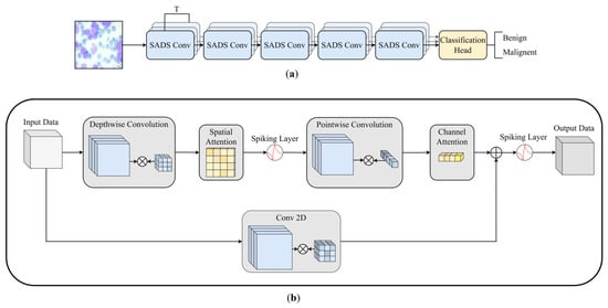
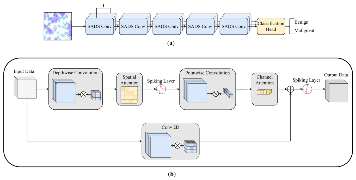
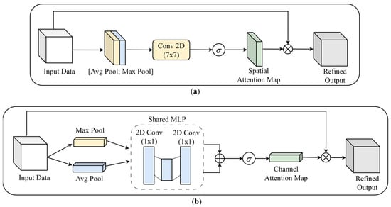
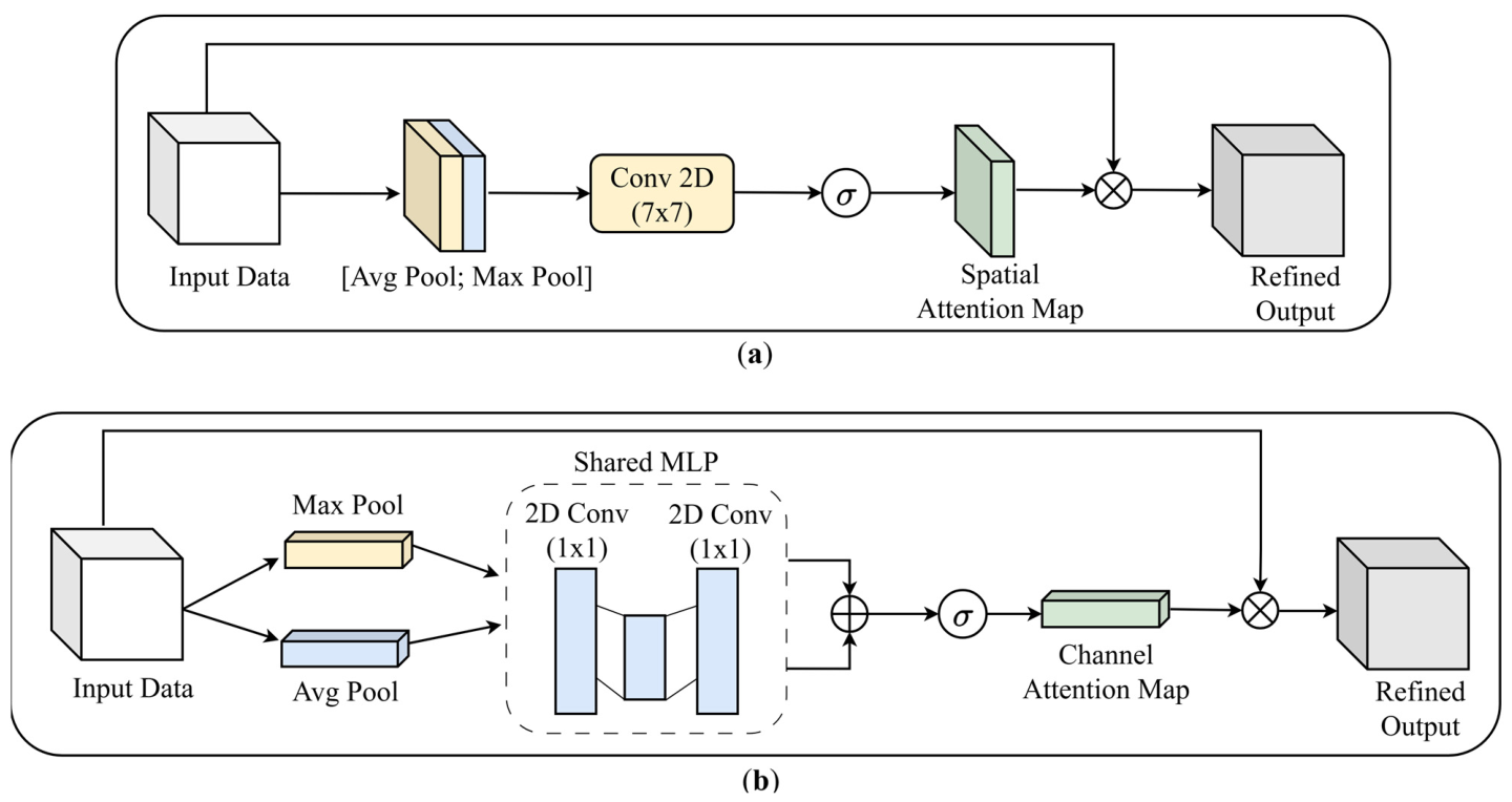
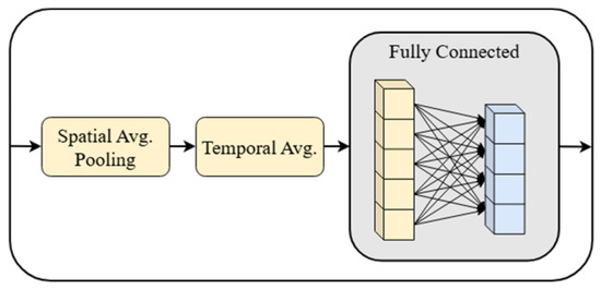
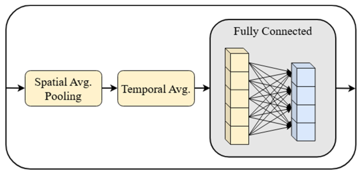
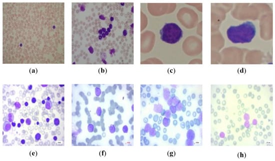
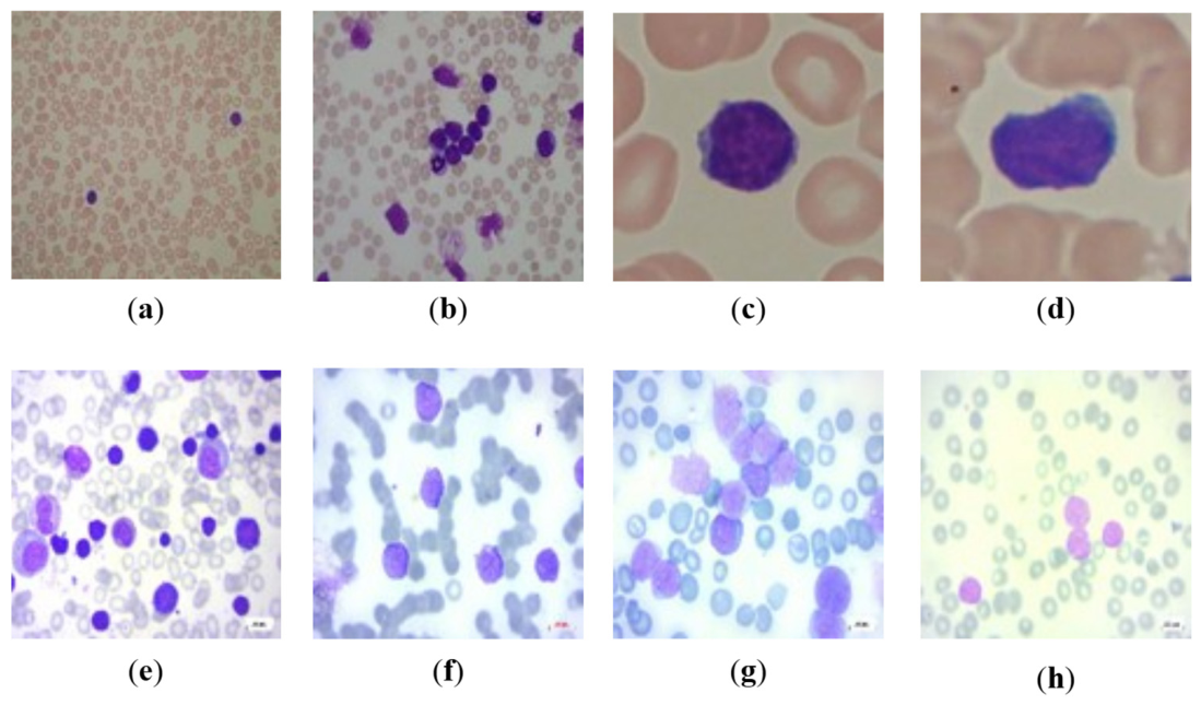
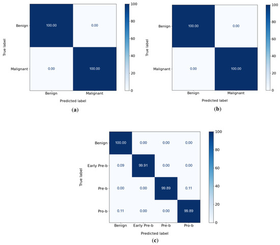
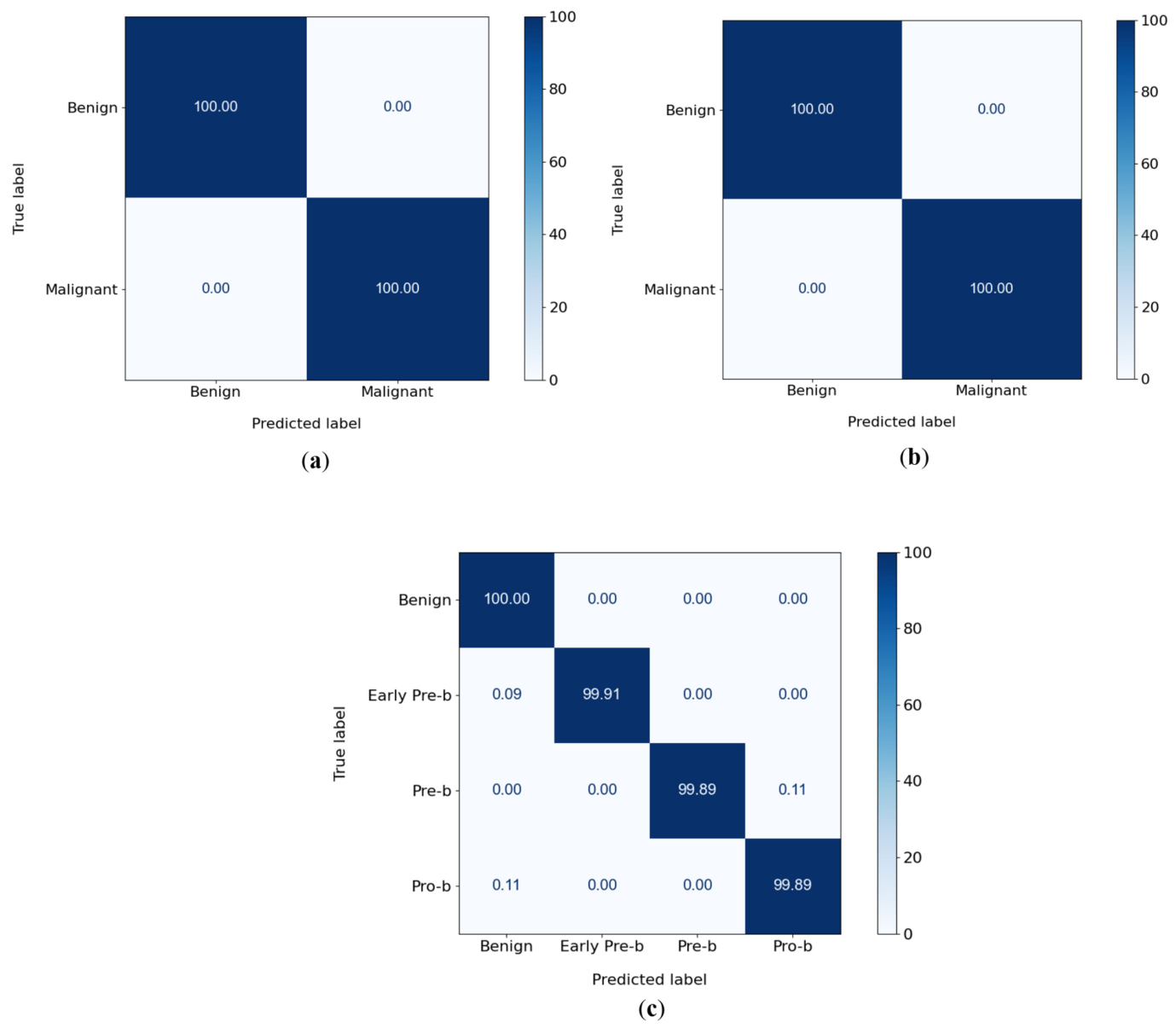
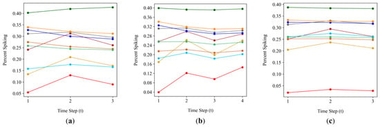
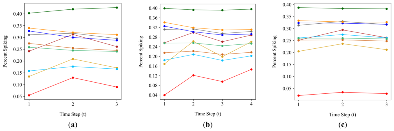
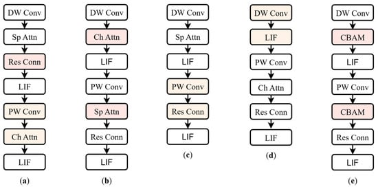
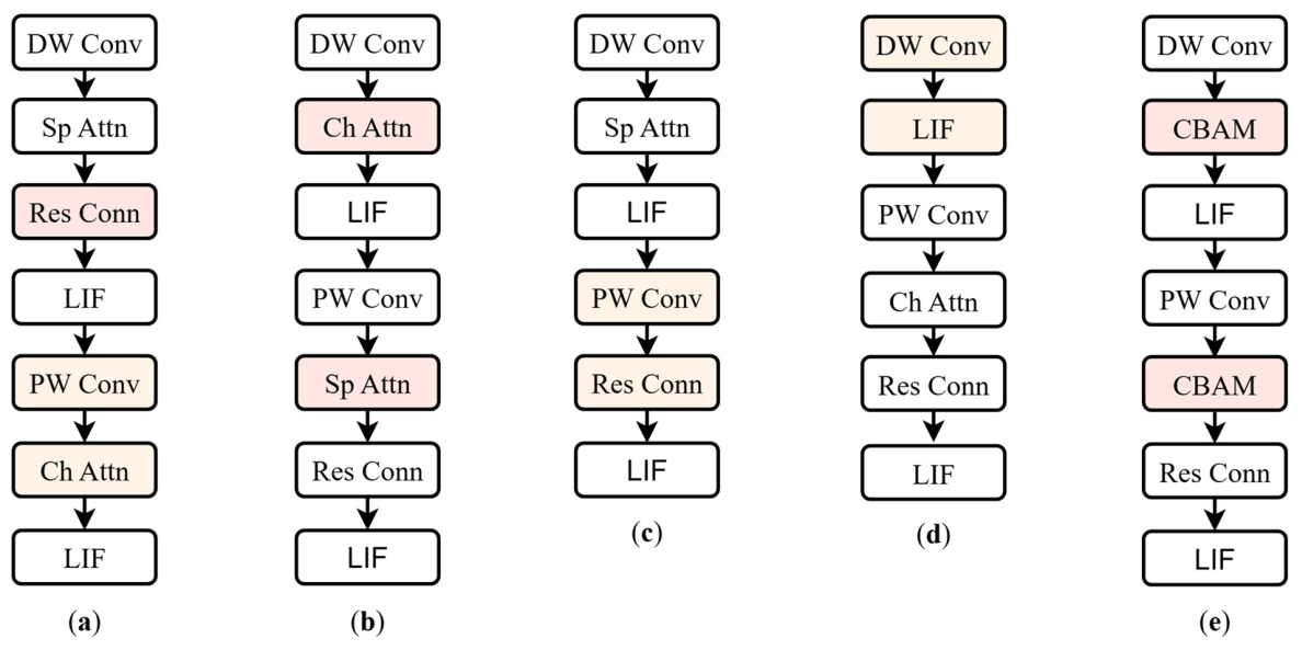
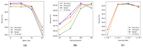
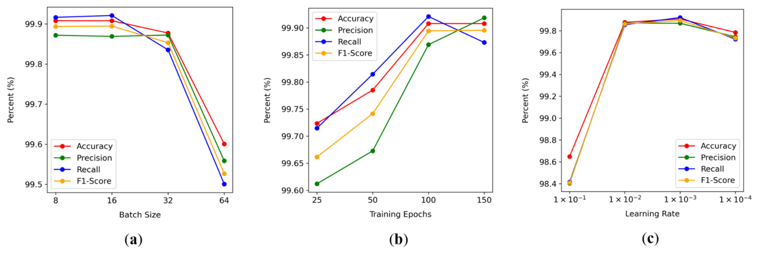
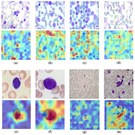
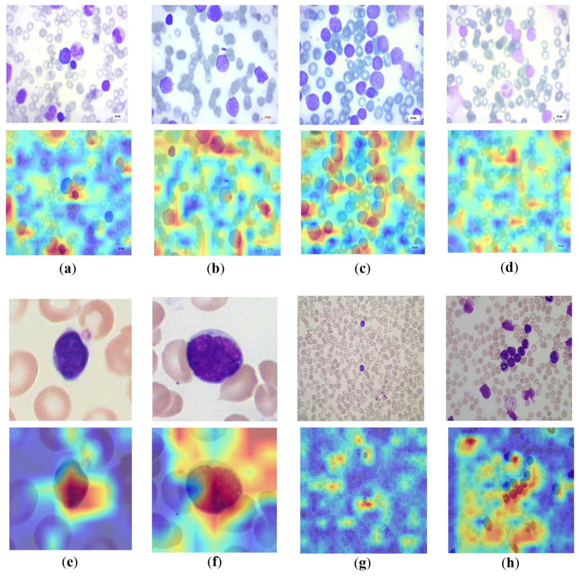

Disclaimer/Publisher’s Note: The statements, opinions and data contained in all publications are solely those of the individual author(s) and contributor(s) and not of MDPI and/or the editor(s). MDPI and/or the editor(s) disclaim responsibility for any injury to people or property resulting from any ideas, methods, instructions or products referred to in the content. |
© 2026 by the authors. Licensee MDPI, Basel, Switzerland. This article is an open access article distributed under the terms and conditions of the Creative Commons Attribution (CC BY) license.