


Abstract
Fused deposition modeling (FDM) is a material-extrusion additive manufacturing technology that is widely used in rapid prototyping, complex product modeling, and functional part fabrication. However, process-parameter drift and environmental disturbances may induce underfilling, overfilling, warping, delamination, and other defects, thereby reducing part quality or interrupting the manufacturing process. Since FDM is characterized by point-wise extrusion and layer-by-layer deposition, layer-surface images naturally contain both spatial morphology and temporal evolution information. Existing image-based diagnostic methods often treat layer images as independent samples, and the selection of the image-stream length is still insufficiently supported by experimental evidence. Moreover, spatial compression in spatiotemporal neural networks may remove local defect information that is important for distinguishing similar process-parameter drifts. This study provides a deployment-oriented analysis of FDM image-stream diagnosis by systematically examining how layer-window length, spatial feature preservation, and strict data partitioning influence process-parameter drift recognition. To address these issues, this paper studies ConvLSTM-based FDM image-stream process-parameter drift diagnosis. Continuous region-of-interest image streams are constructed for one nominal condition and six process-parameter drift conditions. In this paper, the time step T denotes the number of consecutive layer-surface images, or, equivalently, the number of consecutive printed layers, contained in one diagnostic image stream. A ConvLSTM-Flatten baseline is first developed to preserve complete spatial feature maps and to evaluate the effect of different time-step lengths. Then, a ConvLSTM model with adaptive spatial pooling and temporal attention (ASP-TA) is constructed to analyze the influence of spatial pooling granularity and temporal feature fusion. The experiments show that the ConvLSTM-Flatten model achieves the highest average test accuracy of 0.7288 at , whereas is identified as a practical optimal time step when test accuracy, image-frame computation, diagnosis latency, and convergence behavior are considered together. The paired trial-wise accuracy difference between and is small and not statistically significant over ten repeated trials. Thus, the diagnostic window corresponding to covers three consecutive deposited layers; after the initial window is available, stride-one stream construction allows the diagnosis to be updated with each newly acquired layer image. ASP-TA with a pooling size of eight consistently outperforms ASP-TA with a pooling size of four, but both are lower than the Flatten baseline, indicating that preserving sufficient spatial information is essential for distinguishing FDM process-parameter drift states. The results reveal the non-monotonic influence of time-step length and clarify the tradeoff between spatial feature preservation and model compactness in FDM image-stream process-parameter drift diagnosis.
1. Introduction
Additive manufacturing (AM) refers to a group of manufacturing technologies that fabricate parts by accumulating material rather than removing material. Fused deposition modeling (FDM), also known as fused filament fabrication, is one of the most widely used material-extrusion AM processes. Owing to its low equipment cost, user-friendly operation, flexible process implementation, and environmental compatibility, FDM has been extensively applied in rapid prototyping, customized product manufacturing, medical devices, aerospace components, and automotive applications [1,2,3,4]. In a typical FDM process, thermoplastic filament is heated by a liquefier, extruded through a nozzle, and deposited along a predefined tool path. After one layer is completed, the platform moves downward by one layer height, and the deposition process is repeated until the part is formed.
Although FDM has broad engineering potential, the quality of FDM parts is affected by many factors, including nozzle flow rate, printing speed, liquefier temperature, feed-system stability, equipment condition, slicing strategy, and environmental disturbance [5,6,7,8,9]. Such factors may cause under-extrusion, over-extrusion, enlarged pores, filament discontinuity, layer delamination, warping, and surface roughness. These defects not only degrade the mechanical performance and dimensional accuracy of parts but may also interrupt the manufacturing process. Therefore, monitoring the FDM manufacturing process and diagnosing process-parameter drift states are necessary for ensuring part quality and improving process reliability.
The FDM process produces multiple types of data that can be used for monitoring and diagnosis. Vibration signals can reflect the motion status of the nozzle, platform, and frame, and have been used for equipment-state monitoring and fault detection [10,11]. Acoustic emission signals can capture dynamic material changes and have been used to identify nozzle clogging, material shortage, and other process anomalies [12,13]. Temperature signals obtained by thermocouples, thermistors, infrared sensors, or thermal cameras can be used to characterize cooling behavior and thermal history [14,15]. Laser scanners and point-cloud data can measure geometric variation and surface anomalies [16,17]. Multisensor data fusion can improve diagnostic capability by combining complementary information from different sources [10,18,19]. However, these sensing methods often require additional hardware, strict installation conditions, complex synchronization, or high-dimensional data processing.
Compared with the above sensing signals, image-based methods provide a non-contact and high-resolution description of layer morphology. Layer-surface images can directly reveal local pores, material accumulation, filament interruption, rough textures, and other surface defects. Therefore, image-based monitoring and diagnosis have become an important direction in AM quality assurance [20]. According to the form of the image data, existing methods can be broadly divided into single-image methods and image-stream methods.
Single-image methods diagnose the process state by analyzing each layer or each local region independently. Statistical modeling methods divide an image into regions of interest (ROIs), calculate statistical indicators, such as the generalized likelihood ratio (GLR), and construct control charts for monitoring layer-wise quality changes [21,22]. Deep learning methods, especially convolutional neural networks (CNNs), can automatically extract spatial features and have been used for surface defect classification and delamination prediction [23,24]. However, single-image methods usually ignore the temporal dependence between consecutive layers. This limitation becomes more prominent in long-span manufacturing processes, where a transient parameter drift may produce a detectable consequence only after several layers.
Image-stream methods are motivated by the layer-accumulation mechanism of FDM. A small abnormality caused by nozzle clogging, abnormal filling speed, or insufficient material flow may propagate and accumulate over subsequent layers. Such evolution can be reflected in a sequence of layer images. Consequently, image streams provide a natural representation for capturing both intra-layer spatial structure and inter-layer temporal evolution. CNN-LSTM models first use CNNs to extract spatial features from each frame and then use LSTM to model temporal dependence [25,26]. Transformers have also been used for image-stream diagnosis by using space-time attention mechanisms [27]. ConvLSTM integrates convolution into the gating mechanism of LSTM and is specifically designed for data with both spatial and temporal structures [28]. It has been used in AM image-sequence monitoring and defect classification [29,30]. Nevertheless, when ConvLSTM is applied to FDM image-stream diagnosis, two issues require further investigation.
First, the length of the image stream, referred to as the time step in this paper, must be selected carefully. If the time step is too short, the model may not sufficiently capture the spatiotemporal dependency between layers. If the time step is too long, the number of available training samples decreases, redundant historical images may be introduced, and diagnosis latency may increase. Therefore, the relationship between time-step length and diagnostic performance is not necessarily monotonic. Second, spatial feature preservation affects the ability of the model to distinguish visually similar process-parameter drift states. Flattening the ConvLSTM feature map preserves complete spatial information but leads to a high-dimensional classifier. Spatial pooling reduces parameters and may improve compactness, but it can remove local defect cues, such as pore morphology and filament discontinuity. Thus, the influence of spatial pooling granularity should be analyzed in the FDM process-parameter drift diagnosis context.
In this study, a FDM image-stream diagnosis framework is constructed to investigate the influence of the image-stream length and spatial feature preservation on parameter-drift diagnosis. To reduce within-part leakage, the process-parameter drift samples are partitioned by physical parts into training, validation, and testing sets, so the drift-class evaluation uses physical parts not included in training. The nominal class is reported with an explicit qualification because only one standard part is available, and it must be split by ROI. The analysis is then performed with both a ConvLSTM-Flatten baseline and a ConvLSTM-ASP-TA model, so that the effects of time-step length and spatial feature preservation can be studied.
The contributions of this paper are as follows:
- Compared with previous ConvLSTM-based AM monitoring studies that mainly use ConvLSTM as a spatiotemporal classifier, this work explicitly isolates the layer-based time-step length as an experimental factor and evaluates its influence on diagnosis accuracy, Macro-F1, convergence speed, image-frame computation, and error distribution.
- A ConvLSTM-ASP-TA model is constructed by introducing adaptive spatial pooling and temporal attention. The effect of spatial pooling granularity is investigated by comparing pooling sizes and .
- Experimental results show that the time-step effect is non-monotonic and that full spatial preservation is important for distinguishing FDM process-parameter drift classes with similar visual appearances. By jointly analyzing diagnostic performance, convergence behavior, image-frame computation, and stable confusion patterns, this work provides a deployment-oriented basis for selecting image-stream length and spatial representation in FDM visual diagnosis.
The remainder of this paper is organized as follows. Section 2 presents the image-stream construction procedure, data partitioning strategy, ConvLSTM-Flatten model, ASP-TA model, and evaluation metrics. Section 3 describes the experimental data and implementation settings, and reports the diagnosis results and analyzes the effects of time-step length and spatial pooling. Section 4 discusses the implications and limitations of the results. Section 5 concludes this paper.
2. Methodology
2.1. Diagnosis Task and Class Definition
The objective of the diagnosis task is to identify the process state of a FDM part from layer-surface image streams. The task contains one nominal condition and six process-parameter drift conditions. These drift conditions correspond to high and low levels of nozzle flow rate (NFR), filling speed (FS), and liquefier temperature (LT). The class-label definition is shown in Table 1.
Table 1.
Class-label definition of the process-parameter drift states.
2.2. Construction of Image Streams with a Specific Time Step
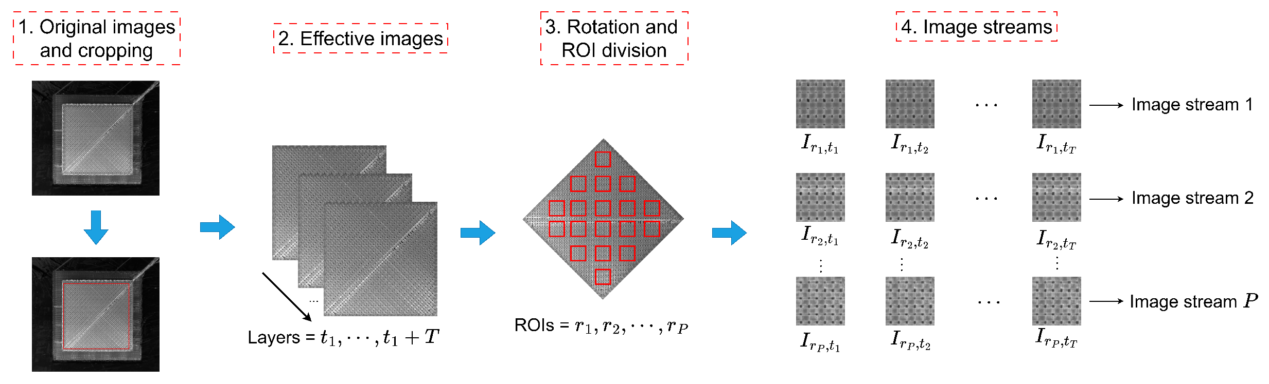
For a FDM part with L valid layers, the construction of image streams with a specified time step T consists of four steps. First, irrelevant background regions are cropped, and the effective part area is retained. Second, continuous cropped layer images are concatenated according to their manufacturing order. In this process, all layer images must have the same size and spatial alignment; otherwise, temporal information between layers may be distorted. Third, image rotation and ROI division are performed. Since the printing path of the experimental FDM part has an angle of approximately 45° relative to the X–Y platform, rotation is used to increase the proportion of filament regions within each ROI and reduce the proportion of holes. Multiple ROIs are extracted from each layer to enlarge the dataset. The same ROI index must correspond to the same spatial position across all layers. Finally, a sliding window is used to construct image-stream samples along the temporal dimension. The construction procedure is illustrated in Figure 1.
Figure 1.
Construction of a FDM image stream with time step T, modified based on [27].
Here, T is not a physical time measured in seconds. It is a dimensionless layer-based window length, namely, the number of consecutive layer-surface images used as one diagnostic sample. Because each layer image is acquired after the corresponding layer has been deposited, T can also be interpreted as the number of consecutive printed layers covered by the diagnostic window. For the sample ending at layer t, the model can output a diagnosis once the latest image is obtained. If the average printing-and-imaging time of one layer is denoted by , the physical duration covered by a T-frame window is approximately . With a stride of , the first stream-based diagnosis can be issued after the initial T layer images have been acquired, and subsequent diagnoses can be updated layer by layer as each new image arrives.
As shown in Figure 1, the ROI construction is intended to keep the same ROI index aligned with the same physical position across consecutive layers. After the printed surface is isolated and aligned, fixed ROI positions are used to track local layer accumulation at corresponding surface regions. The key analysis areas are the ROIs covering deposited filaments, inter-road pores, filament edges, discontinuities, and material-accumulation regions, because these areas carry direct visual evidence of under-extrusion, over-extrusion, temperature-related texture change, and speed-related deposition variation.
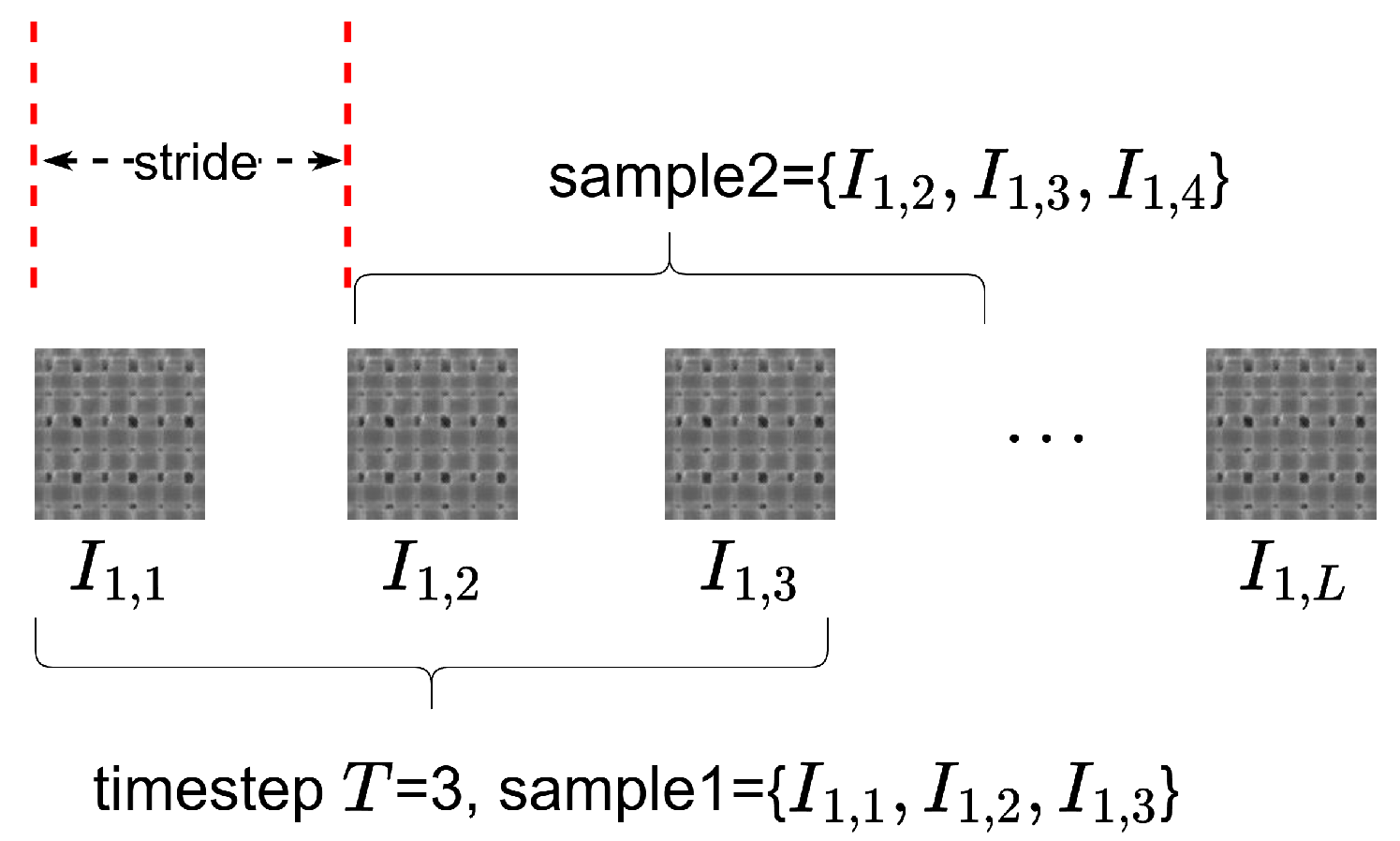
Let P denote the number of ROIs and S denote the stride of the sliding window. Then, the number of image-stream samples generated from one part is illustrated in Figure 2 and given by Equation (1):
Figure 2.
Image-stream samples obtained from a ROI sequence.
In this paper, . For a fixed ROI position, a layer sequence can be denoted by . The image-stream sample ending at layer t is
The label of the image stream is determined by the process state of the latest layer . For a time step T, the total number of image frames participating in the computation is
Therefore, should be considered together with diagnostic accuracy and latency when selecting a practical time-step length.
2.3. Data Partitioning
Because image-stream samples generated from the same physical part are highly correlated, the data partitioning strategy is designed to reduce repeated-texture memorization for the drift classes by separating physical parts whenever multiple parts are available. For the six process-parameter drift classes, process-parameter drift data are split by physical part. For each process-parameter drift class, two parts are used for training, one part for validation, and one independent part for testing. ROI-level partitioning is adopted for the nominal class due to the availability of a single nominal part. Thirty-six ROI positions are extracted from each valid layer. For the nominal class, 28, four, and four ROI positions are assigned to the training, validation, and test subsets, respectively. This nominal-class split is not a true cross-part split; it is retained only to keep the nominal state in the seven-class diagnosis task and is reported as a limitation. The strict partitioning strategy is shown in Table 2.
Table 2.
Strict data partitioning strategy used in this study.
This strategy is adopted to avoid optimistic evaluation caused by overlapping windows, neighboring ROIs, and repeated local textures from the same physical part. For the six process-parameter drift classes, this strategy evaluates whether the model can classify physical parts that were not used during training. The nominal class is different: because only one nominal part is available, its training, validation, and test samples come from different ROI positions of the same physical part rather than from different nominal parts. Therefore, the nominal-class result should not be interpreted as unseen-nominal-part performance, and the seven-class metrics should be considered together with drift-only analyses when robustness is discussed.
After ROI extraction and data splitting, the training, validation, and test subsets contain 460, 220, and 220 ROI-layer sequences, respectively, with 38–41 valid layers. Because a longer T produces fewer sliding-window samples from the same sequence, Table 3 reports representative stream counts and participating image-frame counts.
Table 3.
Image-stream sample volume and participating image-frame volume for representative time steps.
The final class-wise image-stream counts depend on both the number of ROI-layer sequences and the time step T. Table 4 reports the class distribution for and as two representative settings used later in the time-step analysis. These counts were computed from the fixed split plan and the valid-layer counts of each part.
Table 4.
Class-wise image-stream sample counts after ROI extraction for and .
2.4. ConvLSTM-Flatten Model
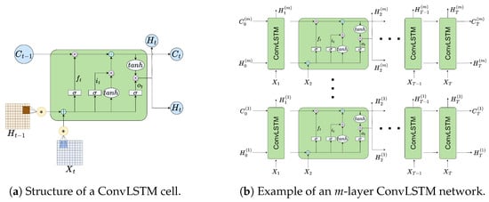
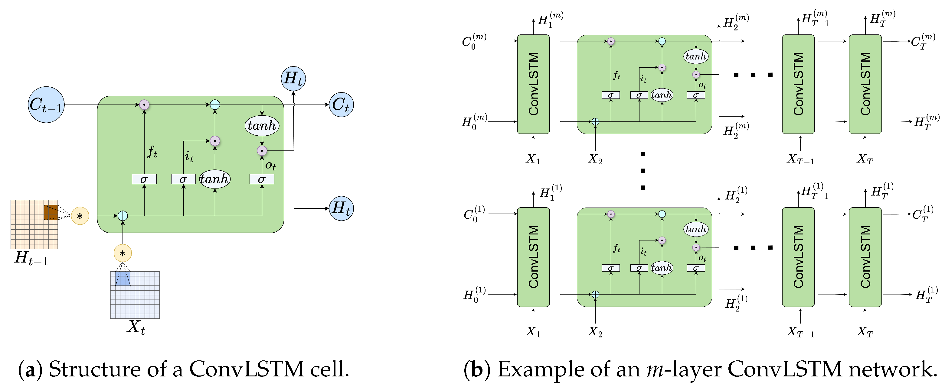
ConvLSTM replaces the fully connected operations in conventional LSTM gates with convolutional operations, allowing it to model spatial and temporal dependencies simultaneously [28]. Let denote the input frame at time t, denote the hidden state, and denote the memory cell. The operator ∗ denotes convolution, and ∘ denotes the Hadamard product. A ConvLSTM cell without explicit peephole connections can be represented by Figure 3a and written as Equation (4). A stacked ConvLSTM network passes the hidden states of each time step from one layer to the next, as illustrated in Figure 3b. This structure increases the representation capacity while keeping the temporal order of the image stream.
Figure 3.
A schematic diagram of a ConvLSTM network.
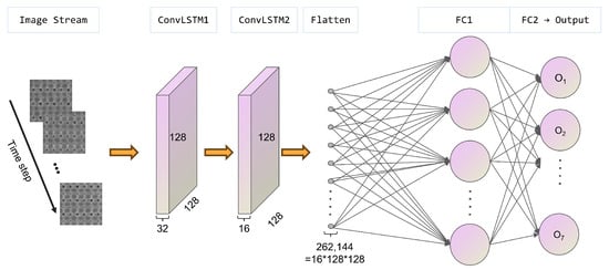
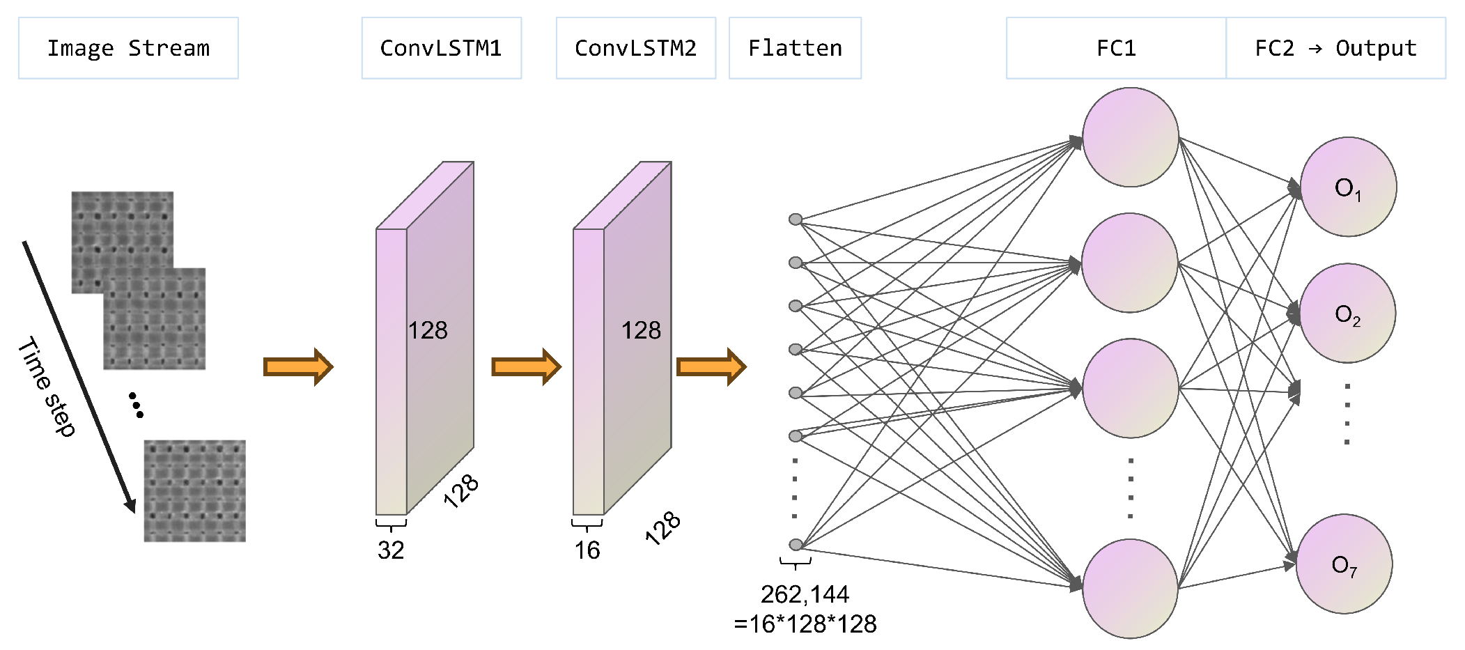
In the ConvLSTM-Flatten model, two stacked ConvLSTM layers form the spatiotemporal feature extractor. The first ConvLSTM layer has 32 output channels with convolution kernels, and the second layer has 16 output channels with kernels. The same padding is used to keep the feature resolution at . The last hidden feature map is flattened into a high-dimensional vector and then fed into fully connected layers for classification:
This structure preserves complete spatial information from the final ConvLSTM feature map, as shown in Figure 4. Its disadvantage is a large, fully connected classifier, but it provides a useful baseline for evaluating whether spatial compression damages defect-related information.
Figure 4.
Structure of the ConvLSTM-Flatten baseline.
2.5. ConvLSTM-ASP-TA Model
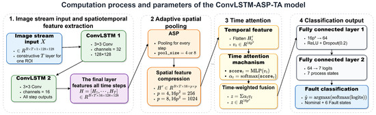
To analyze the effect of spatial compression and temporal feature fusion, a ConvLSTM-ASP-TA model is also constructed. The computational procedure and parameters of the ConvLSTM-ASP-TA model are shown in Figure 5. The model contains a ConvLSTM feature extractor, an adaptive spatial pooling (ASP) module, a temporal attention (TA) module, and a classifier. Given an input stream , the ConvLSTM module outputs hidden feature maps . Each is adaptively pooled to a fixed spatial size , flattened, and projected into a compact vector . The temporal attention module assigns a weight to each time step and fuses the feature sequence into a single representation.
Figure 5.
Computational procedure and parameters of the ConvLSTM-ASP-TA model.
The attention score and normalized weight of time step t are computed as
The pooling size p determines the degree of spatial compression. A smaller p produces a more compact representation but may remove local defect cues; a larger p preserves more spatial details but increases the classifier dimension.
2.6. Experimental Procedure and Metrics
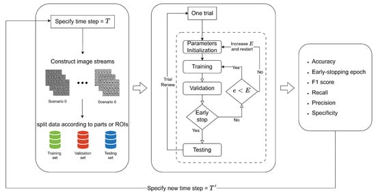
For each time step, the model is trained and evaluated through multiple trials. The hyperparameters, including the batch size, learning rate, kernel size, and early-stopping rule, are kept consistent across time-step experiments so that the time step is the primary variable. The validation set is used for early stopping and model selection, while the test set is used only for final evaluation. The complete experimental procedure for a specified time step is shown in Figure 6 and the algorithm is shown in Algorithm 1.
| Algorithm 1 ConvLSTM-based FDM image-stream diagnosis for a specified time step T |
| Input: Layer-surface images, ROI positions, stride S, time step T, number of trials R. |
| Output: Average diagnostic metrics and standard deviations over R trials. |
|
Figure 6.
Experimental procedure for a specified time step T.
For class c, , , , and denote one-vs-rest true positives, false positives, true negatives, and false negatives. The class-wise metrics are defined in Equation (9), and the corresponding macro-level metrics are obtained by averaging the class-wise values over all classes.
where is the number of classes. The early-stopping epoch is used to characterize convergence speed.
3. Case Study and Analysis
3.1. Experimental Data and Implementation Settings
The experimental data contain one nominal state and six process-parameter drift states generated by adjusting three process parameters: the nozzle flow rate, filling speed, and liquefier temperature. For each drift state, multiple parts are manufactured under different parameter settings, and one additional test part is used for evaluating unseen-part performance within the present dataset. The standard state contains a single part with 40 layers. ROI-level splitting is used only for this standard class because no additional standard parts are available. The process-parameter settings are summarized in Table 5. The layer-surface image data were collected by our research group and have been used in previous image-based statistical process monitoring studies for FDM [27].
Table 5.
Process-parameter settings of seven FDM states.
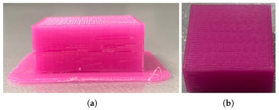
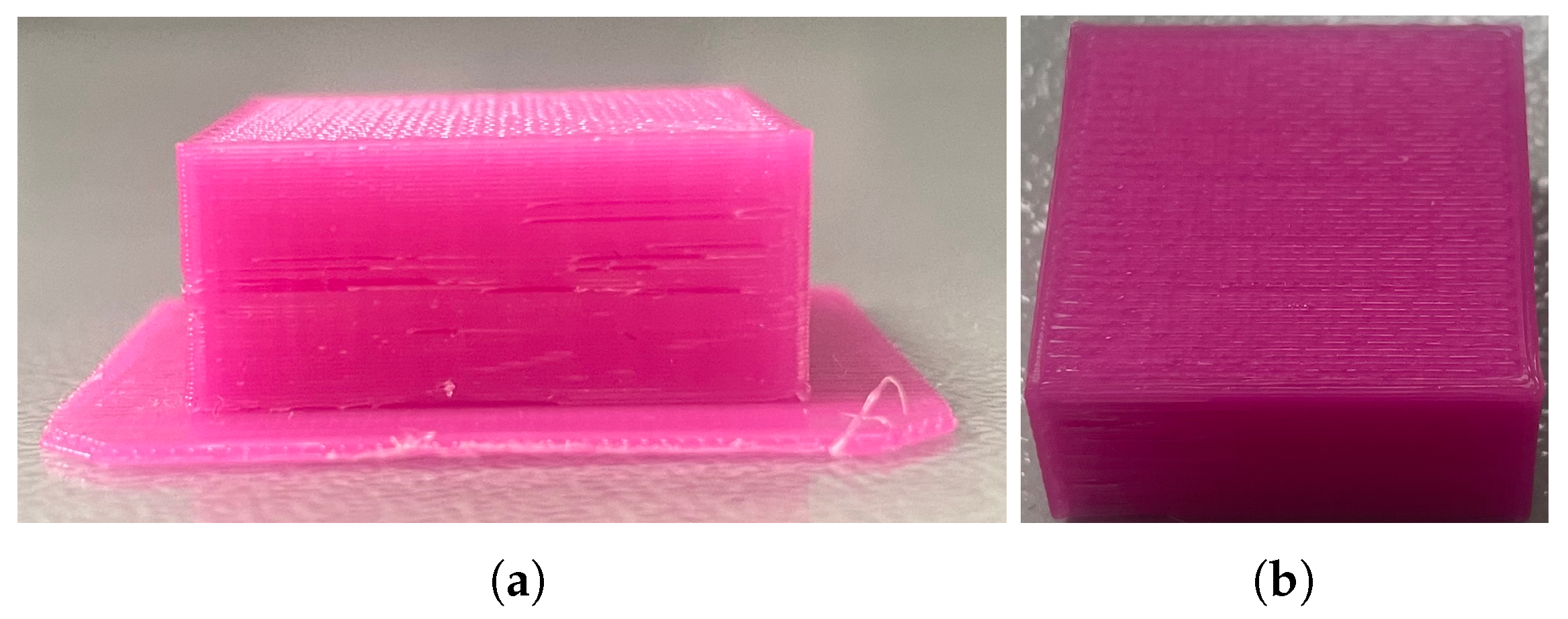
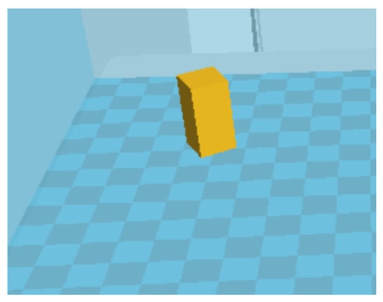
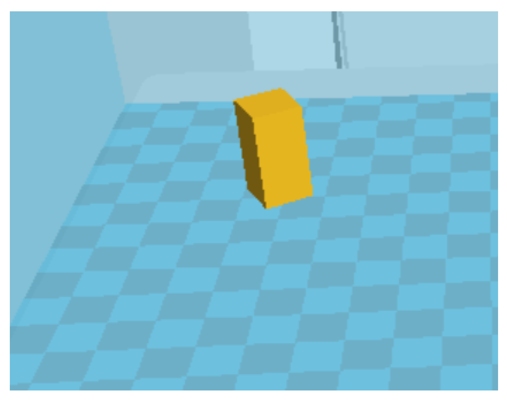
The experiments were conducted on a Hori Z300 FDM printer manufactured in Beijing, China. The printer specification gives a layer-thickness adjustment range of 0.05–0.4 mm and positioning precisions of 0.01 mm, 0.01 mm, and 0.05 mm along the X, Y, and Z axes, respectively. The layer-surface images were grayscale images acquired from above the part using a MicroVision MV–EM510M industrial camera with a resolution of pixels. The material used in the experiments was PLA filament with a 1.75 mm diameter, provided by the printer vendor. The monitored specimen was a rectangular cuboid designed in SolidWorks 2021 and then sliced in Cura to generate G-code. The actual part is shown in Figure 7, and the 3D model is shown in Figure 8.
Figure 7.
The image of the actual FDM part. (a) Side view of the printed part. (b) Slanted top view of the printed part.
Figure 8.
3D model.
Following the image-stream construction procedure in Section 2.2, all images are preprocessed into grayscale ROI images with a size of . For the ConvLSTM-Flatten analysis, time steps from 1 to 37 are tested. Each time step is repeated ten times with different random seeds. For the ASP-TA analysis, time steps are tested with pooling sizes and . The ConvLSTM feature extractor uses two stacked layers with 32 and 16 output channels. Adam is used for optimization. Cross-entropy loss is used for multiclass classification.
To reduce overfitting risk, data were split by physical part for the process-parameter drift classes, and streams from the same physical part were not shared across training, validation, and test subsets. The validation set was used for model selection and early stopping, while the independent test set was used only for final evaluation. In the reported experiments, no random geometric or photometric data augmentation was applied. This avoids introducing augmentation artifacts as potential class cues. Regularization was provided by weight decay (), dropout in the classifier implementation, early stopping with a patience of five validation checks, and repeated trials with different random seeds. These settings reduce the likelihood that the model merely memorizes repeated textures or printer-specific image noise. Nevertheless, because all data were collected from one printer–material–geometry combination, the complete exclusion of machine-specific cues cannot be claimed without cross-printer and cross-material validation.
3.2. Effect of Time-Step Length in ConvLSTM-Flatten
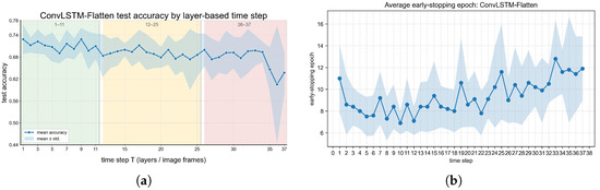
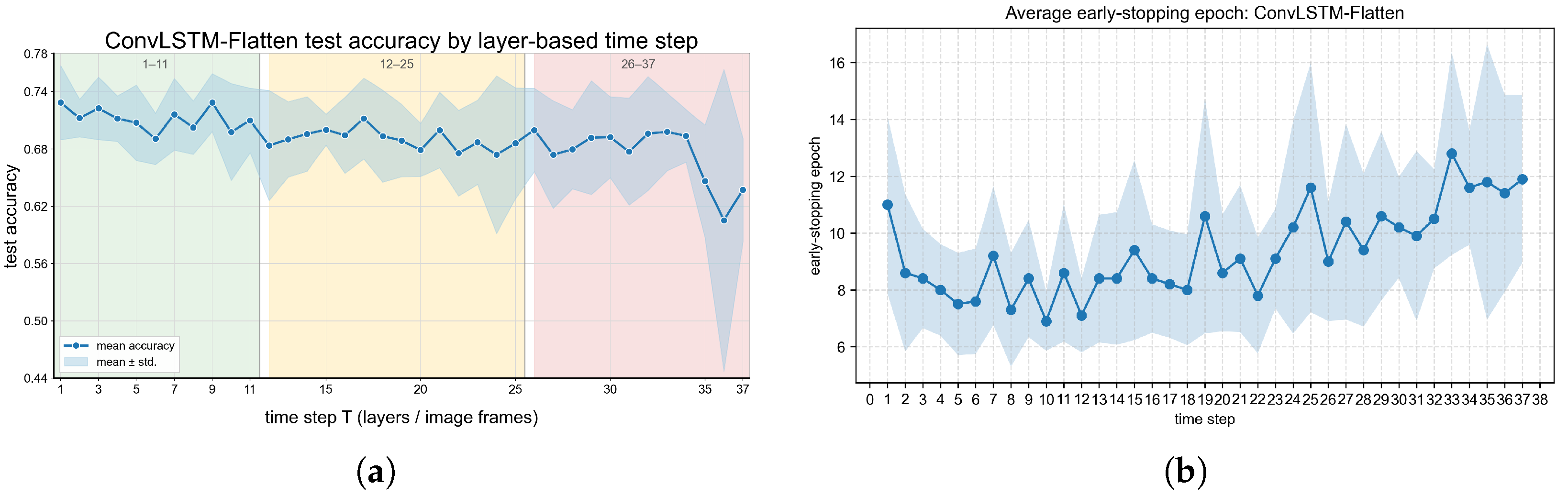
The diagnostic accuracy of ConvLSTM-Flatten under different time steps is shown in Figure 9a. The results reveal a non-monotonic relationship between time-step length and diagnostic performance. Increasing the time step can provide more historical context and improve the model’s ability to learn spatiotemporal dependence. However, after a certain range, a further increase in the time step reduces the number of available training samples and introduces redundant historical information, resulting in decreased accuracy and stability. As shown in Figure 9b, the early-stopping epoch first decreases slightly at short time steps and then shows an overall increasing trend for longer image streams. This suggests that short-to-medium image streams can be optimized with relatively fewer epochs, whereas overly long image streams introduce more temporal information and redundancy, making the optimization process slower and less stable.
Figure 9.
Test accuracy and early-stopping epoch of all ConvLSTM-Flatten trials under different time steps. (a) Mean and standard deviation with selected layer-based time-step ticks. (b) Early-stopping epoch.
Table 6 lists the time steps with relatively high average test accuracy. The best average accuracy is 0.7288 at , followed closely by and . Although achieves the highest average test accuracy, it also involves a larger amount of image-frame computation. According to Equation (3), when , , which increases with T before T approaches approximately . Therefore, among the high-accuracy settings listed in Table 6, uses more participating image frames and leads to a longer diagnostic window. As a supplementary paired comparison across the ten repeated training trials with matched random seeds, the trial-wise accuracy difference was computed as . The mean paired difference was 0.0063, and a paired t-test on these ten differences gave and . When the nominal class was excluded to reduce the influence of the nominal ROI split, the drift-only trial-wise accuracies averaged 0.7188 for and 0.7252 for ; the paired difference remained small and non-significant (, ). This repeated training comparison indicates that, under the present fixed data split, the small mean advantage of over is not stable enough to justify choosing when latency, frame computation, and convergence behavior are also considered. In contrast, although also obtains a high average accuracy, its early-stopping epoch is clearly larger, indicating slower or less stable convergence.
Table 6.
Time steps with relatively high test accuracy in ConvLSTM-Flatten.
Considering the test accuracy, participating image-frame computation, diagnosis latency, and convergence behavior together, is selected as the practical optimal time step in this study. With the layer-based definition of T and stride , a T-frame classifier has an initial diagnostic warm-up of T acquired layer images: can issue the first stream-based decision after the third layer image, whereas can do so after the ninth layer image. After this initial window is available, each newly acquired layer image forms a new stride-one window, so the diagnosis can be updated layer by layer rather than waiting another full T layers for every decision. To further analyze the effect of the time-step range, the time steps are divided into three intervals. As shown in Table 7, the average accuracy and Macro-F1 decrease from the short-to-medium interval to the long interval.
Table 7.
Average performance of ConvLSTM-Flatten in different time-step intervals.
3.3. Class-Level Metrics and Error Concentration
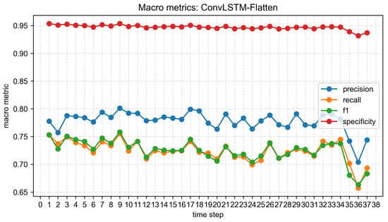
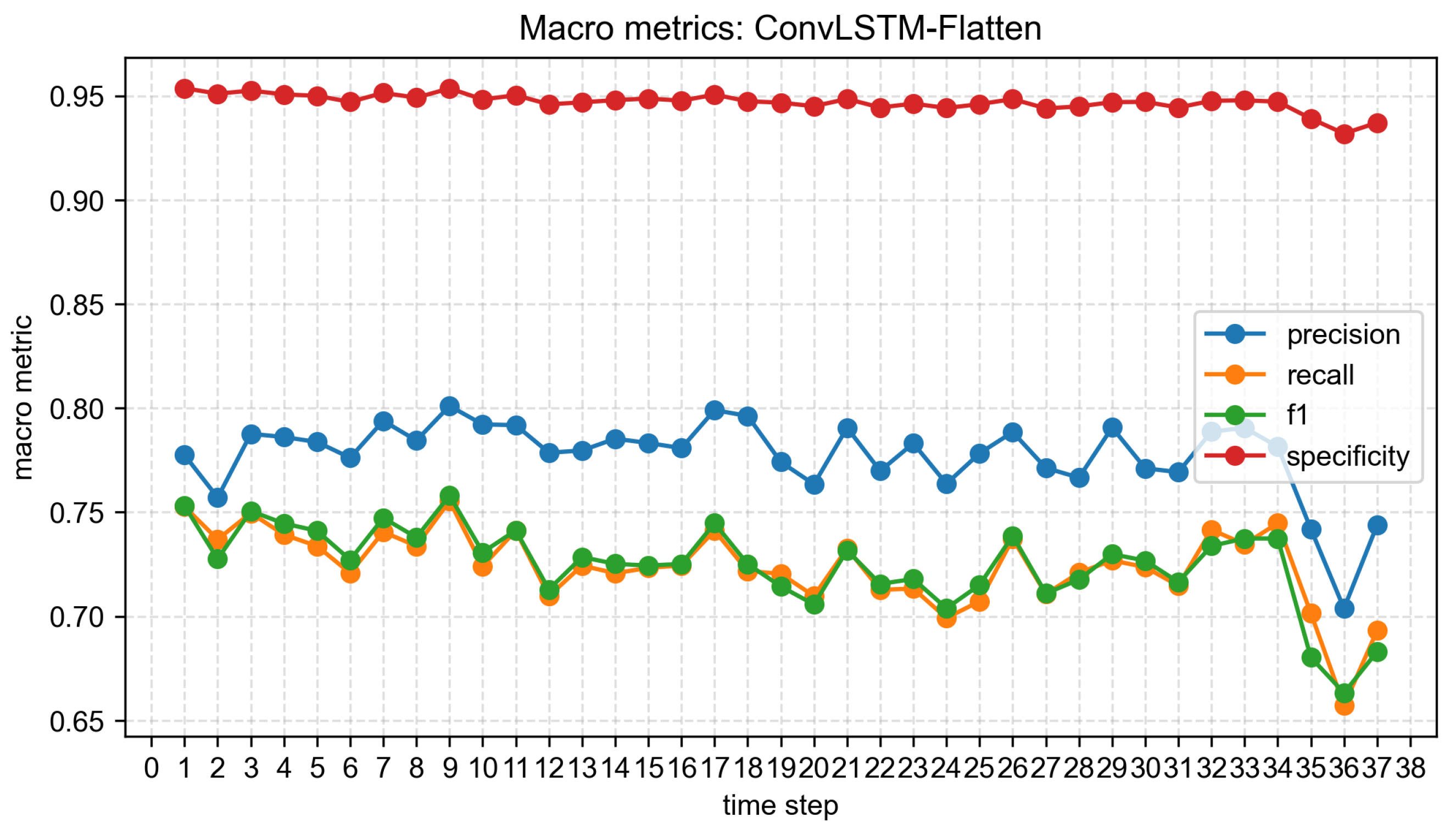
In addition to the accuracy and early-stopping epoch, class-level metrics are analyzed to reveal whether the model performs uniformly across different process-parameter drift states. The macro-level metrics of ConvLSTM-Flatten are shown in Figure 10. The macro-specificity remains high for most time steps, indicating that the model has a strong ability to reject non-target classes in the one-vs-rest evaluation. In contrast, macro-precision, macro-recall, and Macro-F1 mainly fall within a moderate range, showing that the diagnosis difficulty is not evenly distributed among classes.
Figure 10.
Macro-level metrics of ConvLSTM-Flatten under different time steps.
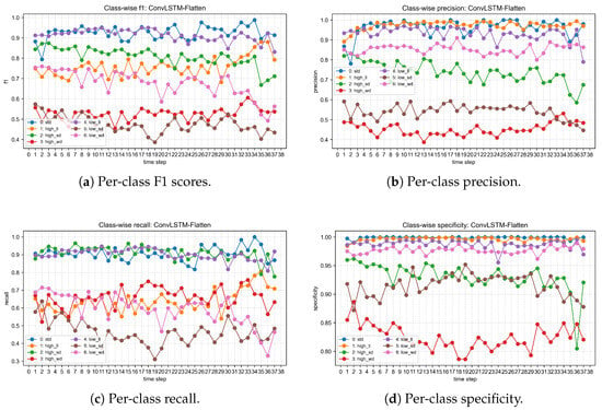
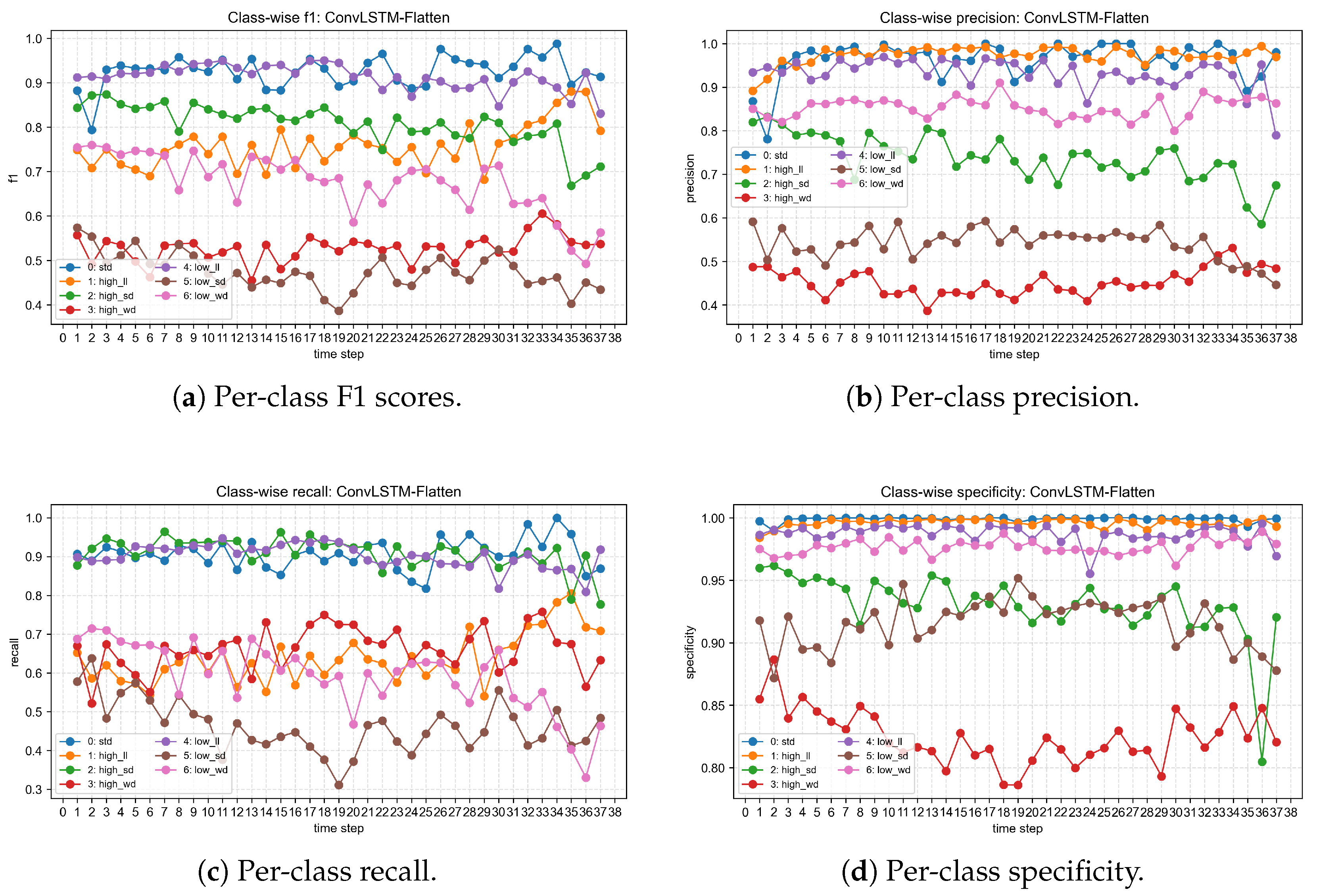
Figure 11 shows the per-class diagnostic performance of ConvLSTM-Flatten under different time steps. The per-class F1 scores are shown in Figure 11a. The nominal, low NFR, and high FS classes maintain relatively high F1 scores across most time steps, whereas high LT and low FS remain difficult. The low LT class shows a moderate but more fluctuating trend, suggesting that its visual representation is more sensitive to the chosen time-step length.
Figure 11.
Per-class diagnostic performance of ConvLSTM-Flatten under different time steps: (a) F1 score; (b) precision; (c) recall; and (d) specificity.
The per-class precision in Figure 11b further shows the reliability of each predicted class. The nominal, high NFR, and low NFR classes have high precision, indicating that samples predicted as these classes are usually reliable. By contrast, high LT and low FS have lower precision, which means that several visually similar drift states are frequently absorbed into these predicted classes.
The recall curves in Figure 11c describe the ability of the model to retrieve true samples from each class. The nominal, high FS, and low NFR classes show relatively high recall, whereas low FS and low LT have weaker recall. This indicates that the model misses many samples from these visually ambiguous classes and assigns them to other drift states.
As shown in Figure 11d, specificity is higher than precision and recall for most classes. However, the high LT class has a visibly lower specificity than the other classes, indicating that non-high LT samples are more likely to be incorrectly predicted as high LT. This result is consistent with the low precision of high LT and suggests that high LT is a strong error-absorbing class in this dataset.
As shown in Table 8, the first four misclassification directions occur under all 37 time steps and dominate the total errors. For example, low FS samples are frequently classified as high LT samples, and high NFR samples are frequently classified as high LT samples. This indicates that the difficulty of the task is not only caused by model capacity but also by the visual similarity between different process-parameter drift states.
Table 8.
Major misclassification directions of the ConvLSTM-Flatten model.
From the viewpoint of defect recognition, the layer-surface images not only provide generic printer-scene texture, but they also contain process-formation evidence associated with the deposited structure, including pore enlargement and pore-shape distortion under insufficient deposition, local material accumulation under excessive flow or high-temperature fluidity, filament-edge discontinuity, rough texture, and nonuniform gray-level distribution along the raster. These features are physically connected with FDM structure formation because they are generated during the extrusion, deposition, spreading, and cooling of the filament [8,31]. The persistent error directions in Table 8 also show that the model mainly confuses states that can produce similar structural manifestations. These stable confusion patterns support the interpretation that the model responds to process-formation cues recorded in layer-wise structural defects, rather than only to isolated printer background noise or incidental scene texture. Specifically, low FS can locally increase heat exposure and material residence time, while high LT directly increases melt fluidity; both conditions may smooth filament edges, modify gray-level texture, and promote local material redistribution, which explains the stable low FS → high LT confusion. Similarly, high NFR and high LT may both generate over-deposition or material accumulation, especially near filament edges, inter-road boundaries, and local pore regions. Therefore, the ROIs that include deposited filaments, filament edges, pores, and accumulation zones are the most relevant regions for interpreting these prediction patterns.
The stability of the dominant error directions is further summarized in Table 9. When the true class is low FS and a misclassification occurs, 93.07% of the errors are assigned to high LT on average. Similarly, 78.74% of high NFR errors are assigned to high LT. These results show that high LT acts as a major absorbing class for visually similar process-parameter drift states.
Table 9.
Average share of major misclassification directions within the corresponding true-class errors.
From the true-class perspective, most errors originate from low FS, low LT, high NFR, and high LT, as shown in Table 10. These four classes account for 90.96% of the top-20 misclassification pairs, confirming that the model performs much better on nominal, low NFR, and high FS states than on visually ambiguous drift states.
Table 10.
Share of true classes in the top-20 misclassification pairs.
From the predicted-class perspective, the errors are mainly absorbed by high LT, low FS, and high FS, as shown in Table 11. High LT alone accounts for 48.02% of the top-20 error pairs, explaining why its precision and specificity are lower than those of most other classes.
Table 11.
Share of predicted classes in the top-20 misclassification pairs.
3.4. Influence of Adaptive Spatial Pooling in ASP-TA
The ASP-TA model is used to investigate whether spatial compression and temporal attention can improve diagnosis performance. Two pooling sizes, and , are compared. A smaller p means stronger spatial compression and fewer parameters, while a larger p preserves more local spatial information. Table 12 shows that consistently outperforms at all tested time steps.
Table 12.
Test accuracy comparison between ASP-TA with and .
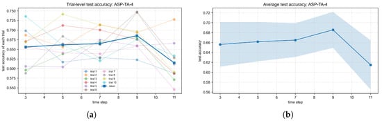
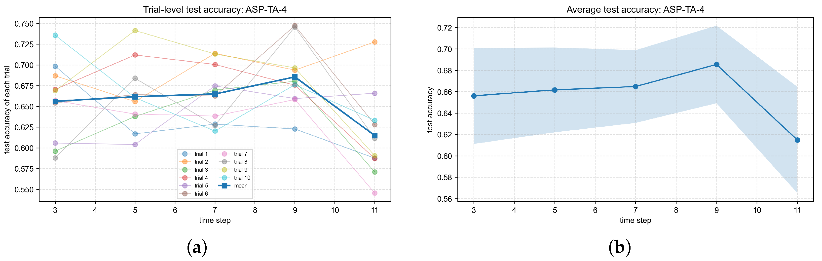
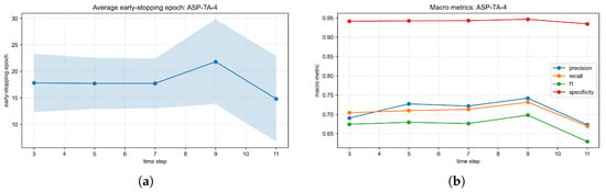
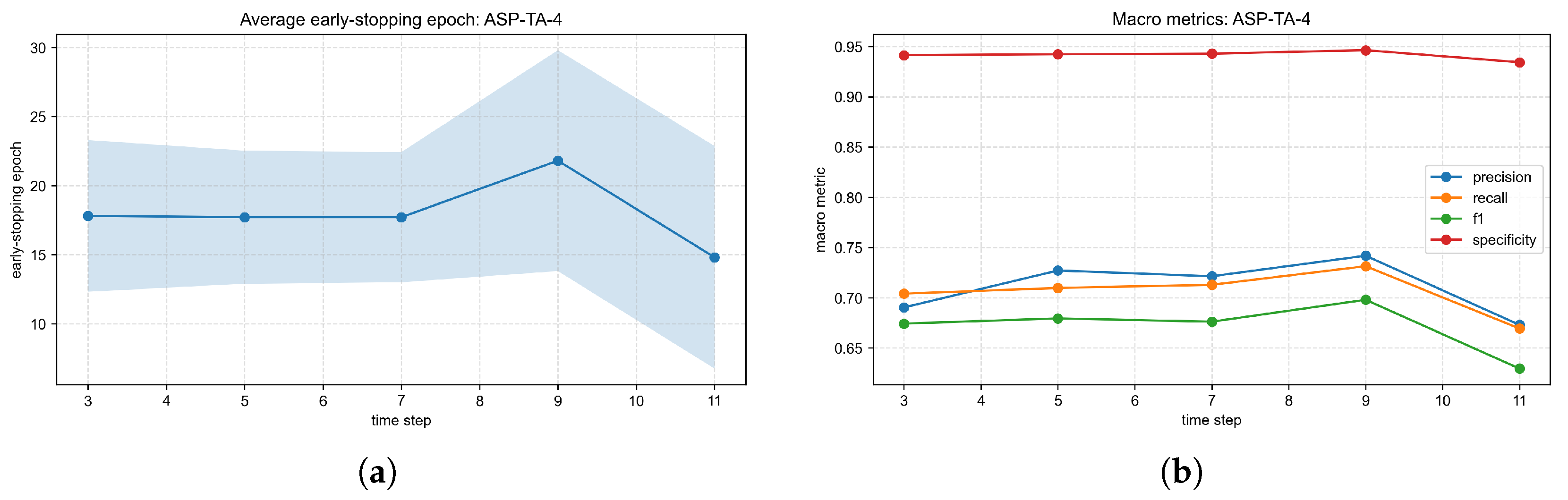
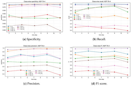
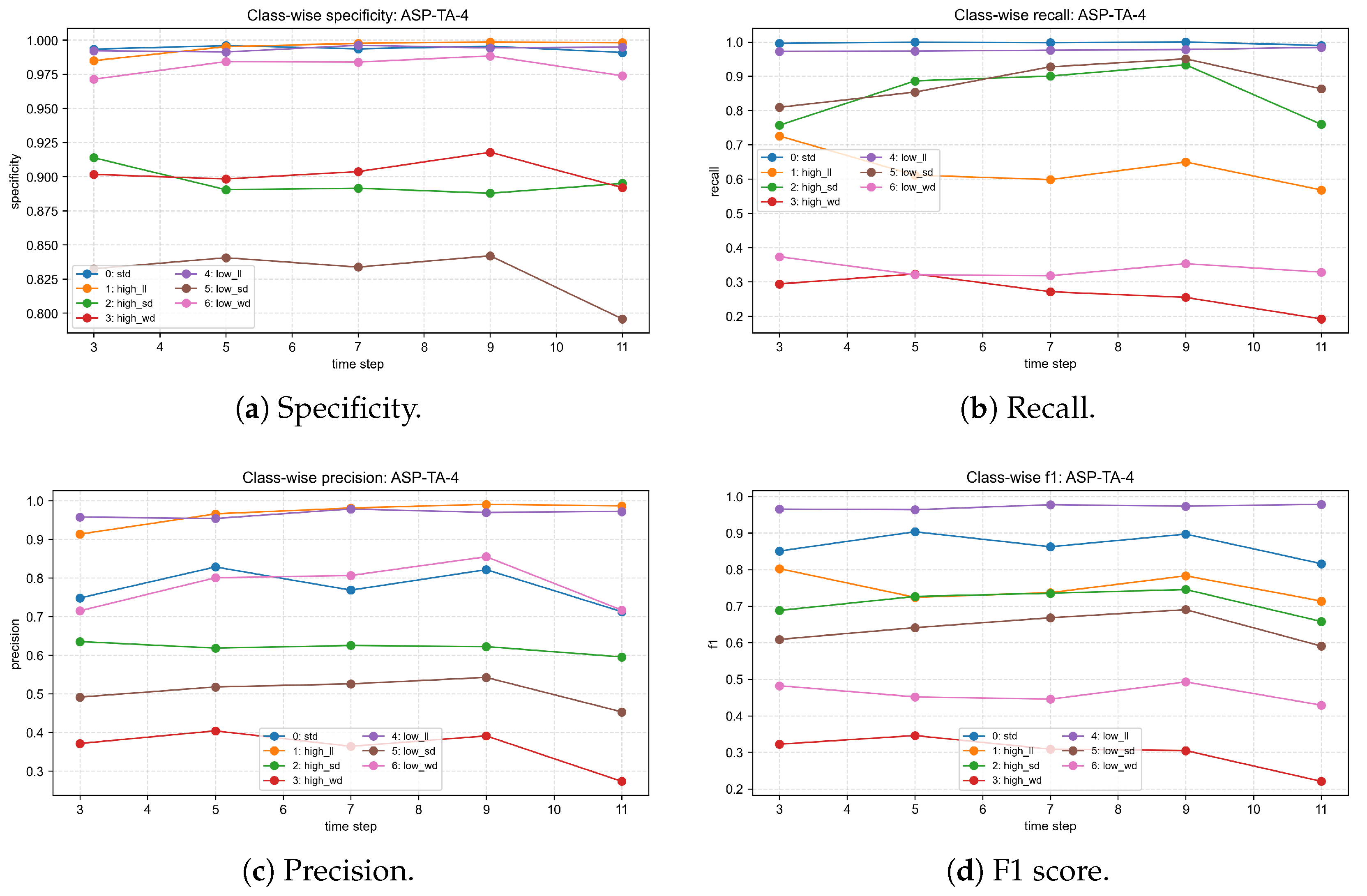
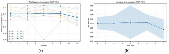
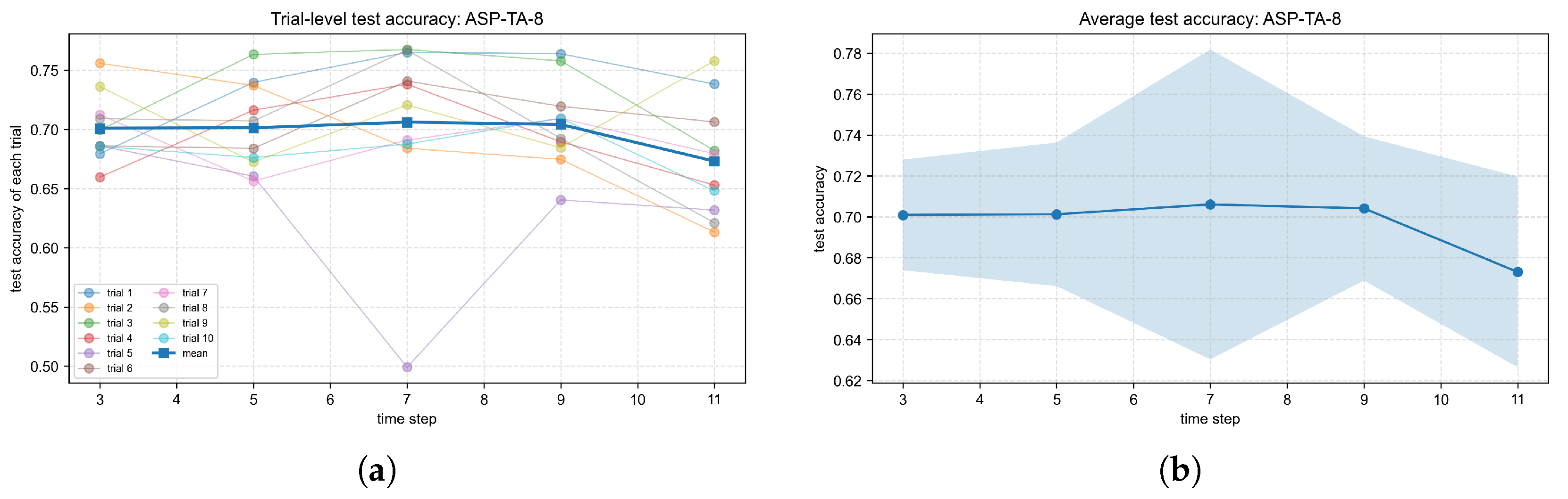
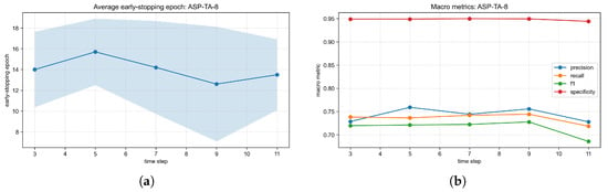
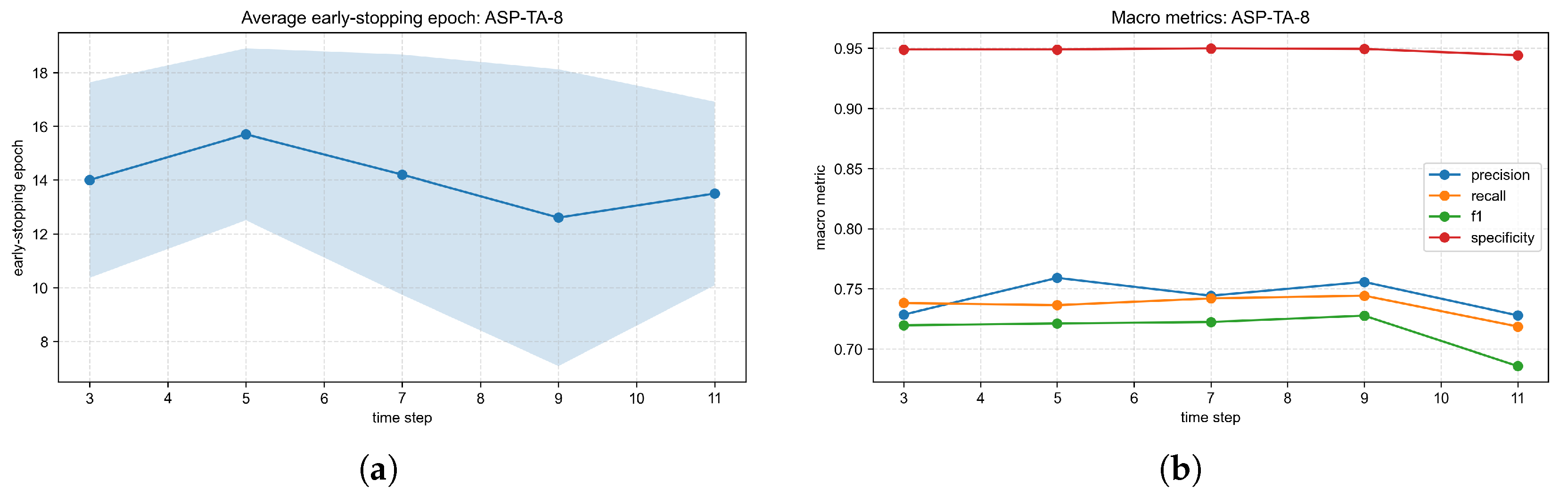
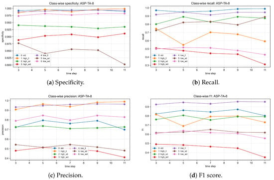
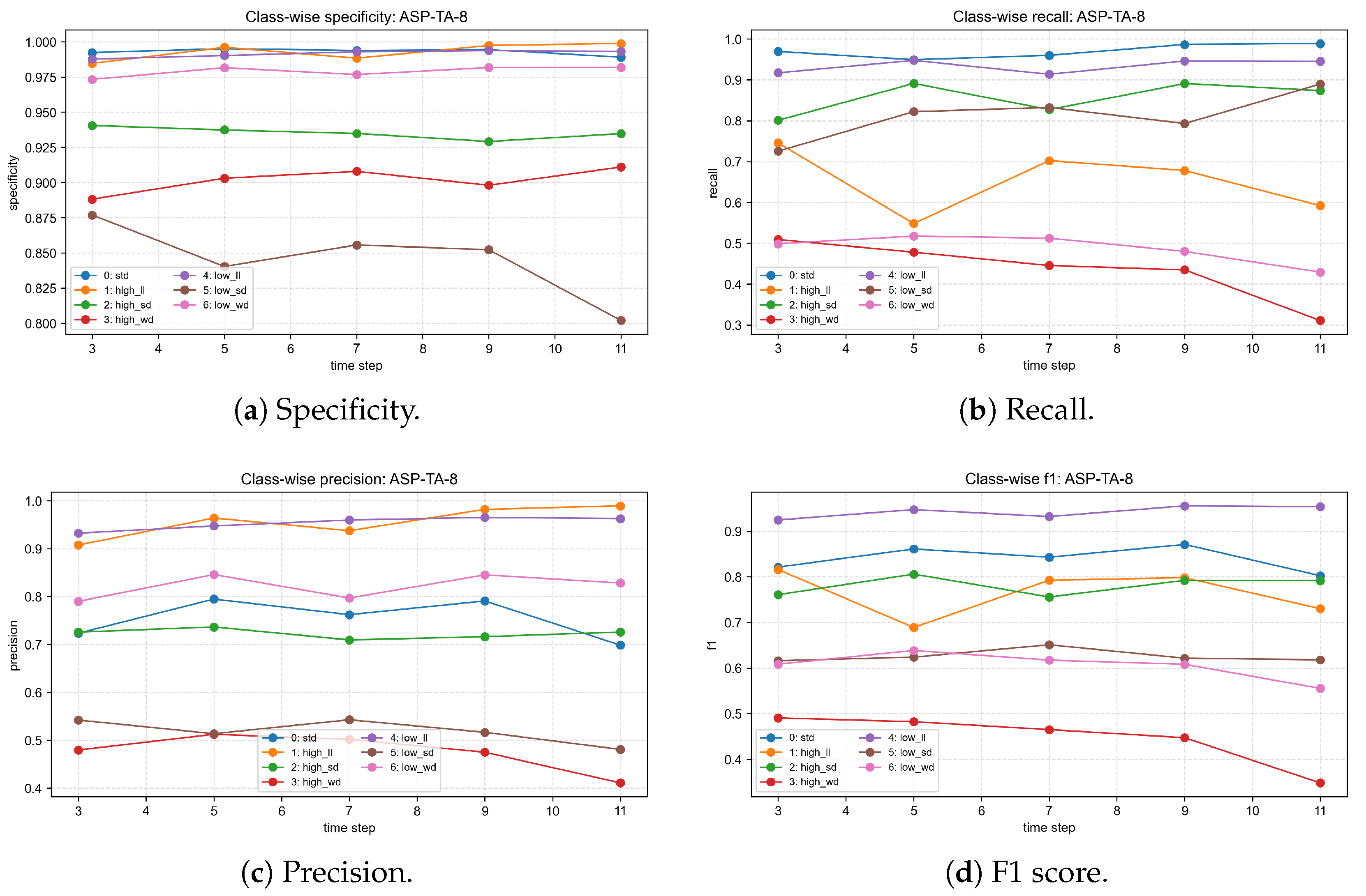
The detailed ASP-TA results in Figure 12, Figure 13, Figure 14, Figure 15, Figure 16 and Figure 17 show that both pooling settings follow a non-monotonic time-step pattern. For , the average test accuracy increases from to and then decreases at . For , the best average accuracy appears at , but gives a more stable combination of accuracy, standard deviation, and Macro-F1. The numerical summary is reported in Table 13.
Figure 12.
Test accuracy of ASP-TA with pooling size . (a) Trial-wise test accuracy for ASP-TA with . (b) Mean and standard deviation of test accuracy for ASP-TA with .
Figure 13.
Convergence and macro-level performance of ASP-TA with pooling size . (a) Early-stopping epoch for ASP-TA with . (b) Macro-level metrics for ASP-TA with .
Figure 14.
Per-class metrics of ASP-TA with pooling size .
Figure 15.
Test accuracy of ASP-TA with pooling size . (a) Trial-wise test accuracy for ASP-TA with . (b) Mean and standard deviation of test accuracy for ASP-TA with .
Figure 16.
Convergence and macro-level performance of ASP-TA with pooling size . (a) Early-stopping epoch for ASP-TA with . (b) Macro-level metrics for ASP-TA with .
Figure 17.
Per-class metrics of ASP-TA with pooling size .
Table 13.
ASP-TA performance under different time steps and pooling sizes.
The improvement from to indicates that local spatial details are important for FDM image-stream diagnosis. Defect-related cues, such as pore distribution, filament-edge discontinuity, and material accumulation, may occupy only a small region within a ROI. Excessive pooling can weaken or remove such cues, making it harder for the classifier to distinguish similar classes.
3.5. Comparison Among ConvLSTM-Flatten and ASP-TA Models
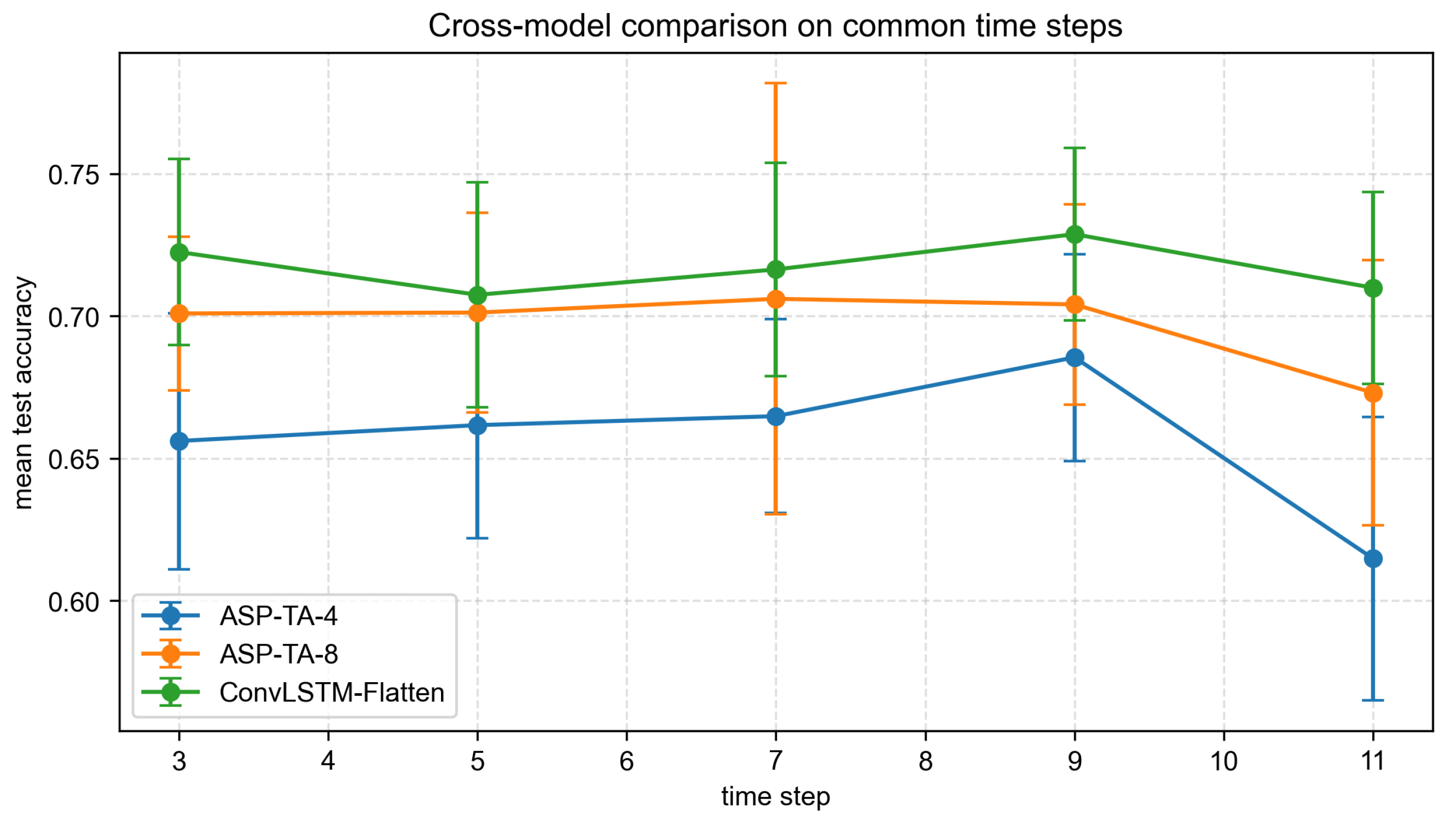
Table 14 and Figure 18 compare the three models under common time steps. ConvLSTM-Flatten obtains the highest accuracy under all five common time steps. ASP-TA with is consistently better than ASP-TA with , but it is still lower than ConvLSTM-Flatten, as indicated by the bold values, which denote the best performance. This finding suggests that the main advantage of ConvLSTM-Flatten comes from its complete spatial feature preservation.
Table 14.
Test accuracy comparison among three models under common time steps.
Figure 18.
Test accuracy comparison among the three models under common time steps.
From the structural perspective, this result indicates that spatial information preservation is important for FDM image-stream diagnosis. Local pores, filament discontinuities, material accumulation, and texture distortions often occupy only small regions in a ROI. The Flatten baseline preserves the full spatial layout of the final hidden feature map, whereas ASP-TA compresses the feature map before temporal attention. Although retains more spatial structure than , both ASP-TA variants still discard more fine-grained spatial information than the Flatten baseline. Therefore, temporal attention alone cannot fully compensate for the loss caused by excessive spatial pooling.
The early-stopping results in Table 15 show that ConvLSTM-Flatten converges faster than both ASP-TA variants. This may be because the Flatten baseline directly feeds complete spatial maps to the classifier, making defect-related local patterns easier to separate under this dataset. In contrast, ASP-TA first compresses spatial features and then learns temporal weights; this structure is more compact but may require more epochs to obtain discriminative representations.
Table 15.
Early-stopping epochs of the three models under common time steps.
3.6. Non-Recurrent Global-Attention Comparison Experiment
To separate the effect of image-stream length from the recurrent memory mechanism of ConvLSTM, a non-recurrent temporal global-attention comparison experiment was conducted. The purpose of this comparison is to test whether long-window degradation persists when ConvLSTM recurrence is removed while temporal global modeling is retained. This experiment serves as an auxiliary analysis rather than a newly proposed architecture.
As shown in Figure 19, the control model first applies a shared CNN frame encoder to each frame in the ROI image stream. The frame-level embeddings are then combined with positional encoding and a classification token and passed to a Transformer encoder, so that all time steps can attend to one another through temporal global self-attention. Finally, the classification token is fed into a fully connected classifier to predict the process-parameter drift class. In the implementation, the Transformer encoder used two layers, four attention heads, an embedding dimension of 128, and a feed-forward dimension of 256.
Figure 19.
Structure of the CNN frame encoder and temporal Transformer.
The experiment used the same split plan, ten trial seeds, stride-one stream construction, early-stopping rule, and independent test protocol as the ConvLSTM-Flatten experiments. The selected time steps were : is the practical short diagnostic window, is the highest-accuracy ConvLSTM-Flatten window, and represent the long-window region. The numerical results are summarized in Table 16.
Table 16.
Results of the non-recurrent temporal global-attention comparison experiment under selected time steps.
The global-attention control did not reverse the long-time-step degradation. Its average test accuracy decreased from 0.6336 at and 0.6068 at to 0.5541, 0.5030, 0.4799, and 0.4991 at , respectively. Because this control removes ConvLSTM recurrence, the decline at long image-stream windows should not be attributed solely to the recurrent memory limitation of ConvLSTM. The result is more consistent with a combined effect of a reduced stream-sample size, redundant historical layer images, optimization instability under the present data scale, and increased diagnostic delay. At the same time, this control should not be interpreted as a general claim that Transformer-based FDM diagnosis is ineffective, because the control was not extensively architecture-tuned.
4. Discussion
The results provide three insights for FDM image-stream diagnosis. First, time-step length has a non-monotonic effect. A short image stream may not fully exploit inter-layer information, while an overly long image stream reduces the sample size and may introduce redundant information. Under the strict data partitioning scheme, gives the highest average accuracy, while provides a more practical choice when test accuracy, image-frame computation, diagnosis latency, and convergence behavior are considered together. Overall, the interval generally outperforms longer intervals. This finding is consistent with the broader view that AM image streams are useful because they encode layer-wise evolution, but that the stream representation must be matched to the defect-evolution time scale and the available sample size [27,32]. The non-recurrent global-attention comparison in Section 3.6 gives the same practical implication: a temporal global-attention architecture can access all frames in the sequence, but long windows still produced lower accuracy under the present split and data scale. This supports the interpretation that the time-step effect is a data-and-process-window issue rather than only a ConvLSTM memory issue.
The present work and the previous time-series Vision Transformer study on FDM parameter-drift diagnosis [27] have different but complementary meanings. The previous study mainly answered an architecture question: whether cross-space-time attention can exploit reconstructed layer-wise image streams, and it reported 0.908 ± 0.031 accuracy with image streams of length and . In contrast, the present study answers a process-diagnosis question: how many consecutive layer images should be used for timely diagnosis of process-parameter drifts, and how the diagnosis can be connected to practical parameter-adjustment guidance. The two studies both use 36 cropped ROIs of size , but their protocols are not directly interchangeable. The present work uses stride-one image streams, fixes a stricter part-level split for the drift classes, explicitly discusses the ROI-split limitation of the nominal class, and systematically varies T from 1 to 37 for ConvLSTM-Flatten. Therefore, the contribution of the present work is not to replace the Transformer architecture, but to provide a deployment-oriented analysis of layer-window length, initial diagnostic warm-up, spatial-feature preservation, and parameter-specific corrective actions. These aspects are the main advantages of the present study for process monitoring and closed-loop decision support.
Second, spatial feature preservation is crucial. Although adaptive spatial pooling reduces the number of parameters, excessive spatial compression weakens local defect cues. The comparison between and confirms that a larger pooled feature map retains more useful information. The superiority of ConvLSTM-Flatten further indicates that complete spatial maps are valuable for distinguishing visually similar process-parameter drift classes in the present FDM dataset. This agrees with image-based and point-cloud-based AM monitoring studies showing that local geometric or surface anomalies, such as pores, bulges, dents, or filament interruptions, often occupy limited spatial regions and can be weakened by excessive aggregation [16,17,33].
Third, several misclassification directions remain stable across time steps. This suggests that some FDM parameter drifts produce inherently similar visual manifestations. For example, low filling speed and high liquefier temperature may both change filament texture and local material distribution, while high nozzle flow and high liquefier temperature may both lead to material accumulation. Therefore, future models should combine image-stream learning with process-mechanism constraints or causal feature learning to distinguish similar root causes. Such a direction is also consistent with process–structure–property modeling, mechanics-based hybrid learning, optimization-assisted structural damage identification, and causal or explainable learning studies, which emphasize that data-driven predictions become more reliable when they are constrained by mechanism-related features, mechanics-derived response variables, or causal representations rather than by incidental visual correlations [34,35,36,37,38].
The results also suggest practical printing recommendations for reducing defects. First, a short diagnostic window, such as , is preferable for an online warning because it preserves most of the diagnostic accuracy while shortening the initial diagnostic warm-up before an intervention can be considered. Second, because the true parameter drift is unknown during online monitoring, corrective actions should be selected according to the drift class diagnosed from the image stream. If the model diagnoses high NFR, the operator should inspect over-extrusion and local material accumulation and then reduce the flow rate toward the nominal setting. If the model diagnoses low NFR, the operator should inspect pore enlargement, filament discontinuity, possible nozzle clogging, or feeding instability and then increase the effective material supply or restore the flow rate toward nominal. If high FS is diagnosed, the filling speed should be reduced toward the nominal setting to avoid insufficient deposition per unit path length. If low FS is diagnosed, the filling speed should be increased toward nominal while checking whether excessive local deposition or heat accumulation has occurred. If high LT is diagnosed, the liquefier temperature should be reduced toward the recommended range to avoid excessive fluidity and material accumulation. If low LT is diagnosed, the liquefier temperature should be increased toward the recommended range to improve melting, spreading, and inter-road bonding. Third, the visual monitoring setup should preserve fine spatial details by using stable illumination, a fixed camera position, and consistent ROI alignment, because excessive spatial compression or image registration drift can hide small pores and filament-edge defects. These recommendations use the model as an early warning and decision-support tool. Image-analysis-based fault diagnosis and correction, including serial-communication-driven closed-loop FDM control, has been demonstrated in recent studies [17,39,40]; however, operator confirmation or validated closed-loop control rules are still needed before automatic parameter correction is deployed in the present setup.
The limitations of this study should also be noted. The dataset is collected from a specific FDM platform, material, geometry, and parameter range. Although the drift-class split by physical part reduces within-part leakage, the experimental population is still limited: only one nominal part is available, each drift class contains a limited number of physical parts, and the nominal class has to be split by ROI. Consequently, the results demonstrate performance under the present printer–material–geometry population and parameter range; broader validation across different printers, materials, geometries, and additional nominal parts is required before wider engineering generalizability can be claimed. In addition, only two pooling sizes are tested for ASP-TA, and more flexible multi-scale temporal and spatial attention mechanisms may further improve performance.
5. Conclusions
This paper investigated FDM image-stream process-parameter drift diagnosis using ConvLSTM-based models. The ConvLSTM-Flatten baseline achieved the highest average test accuracy of 0.7288 at , while was selected as the practical optimal time step after jointly considering test accuracy, image-frame computation, diagnosis latency, and convergence behavior. The paired comparison of trial-wise accuracy differences further indicates that the mean difference between and is small and not significant under the ten matched-seed repeated trials, supporting the use of as a practical rather than purely accuracy-maximizing choice. The average performance decreased from the short-to-medium time-step interval to the long interval, confirming that longer image streams do not necessarily lead to better diagnosis. The non-recurrent global-attention comparison also showed decreasing performance at longer windows, indicating that this trend is not solely caused by the recurrent memory mechanism of ConvLSTM. The ASP-TA experiments showed that consistently outperformed , indicating that stronger spatial preservation is beneficial. However, both ASP-TA variants were inferior to ConvLSTM-Flatten under common time steps, suggesting that complete spatial features remain important for this FDM process-parameter drift diagnosis task. Error analysis further showed that several drift-state pairs, such as low FS to high LT and high NFR to high LT, are persistently confused because of similar visual manifestations.
Future work will focus on adaptive time-step selection, multi-scale spatiotemporal modeling, local spatial attention, and process-mechanism-guided feature learning. Additional datasets from different printers, materials, geometries, process conditions, and nominal parts will also be needed to evaluate the engineering generalizability of the proposed diagnostic strategy.
Author Contributions
Conceptualization, S.W. and T.H.; methodology, S.W. and T.H.; software, S.W.; validation, S.W.; formal analysis, S.W.; investigation, S.W.; resources, T.H. and S.Y.; data curation, S.W.; writing—original draft preparation, S.W.; writing—review and editing, T.H. and S.Y.; visualization, S.W.; supervision, T.H. and S.Y.; project administration, T.H. and S.Y. The author confirms sole responsibility for the study conception and design, data collection, analysis and interpretation of results, and manuscript preparation. All authors have read and agreed to the published version of this manuscript.
Funding
This research received no external funding.
Data Availability Statement
The data presented in this study are not publicly available due to laboratory data-management restrictions. Requests for access to the data can be directed to the corresponding author and will be considered on a case-by-case basis.
Conflicts of Interest
The authors declare no conflicts of interest.
References
- Winarso, R.; Anggoro, P.; Ismail, R.; Jamari, J.; Bayuseno, A. Application of Fused Deposition Modeling (FDM) on Bone Scaffold Manufacturing Process: A Review. Heliyon 2022, 8, e11701. [Google Scholar] [CrossRef] [Scilit]
- Oleksy, M.; Dynarowicz, K.; Aebisher, D. Rapid Prototyping Technologies: 3D Printing Applied in Medicine. Pharmaceutics 2023, 15, 2169. [Google Scholar] [CrossRef] [Scilit]
- Zhang, H.; Hui, J.; Lv, J.; Lee, C.H.; Yan, Z.; Wang, J.; Guo, L.; Xu, Z. A Novel Method to Combine Fused Deposition Modelling and Inkjet Printing in Manufacturing Multifunctional Parts for Aerospace Application. J. Mater. Res. Technol. 2023, 24, 4405–4426. [Google Scholar] [CrossRef] [Scilit]
- Yang, J.; Li, B.; Liu, J.; Tu, Z.; Wu, X. Application of Additive Manufacturing in the Automobile Industry: A Mini Review. Processes 2024, 12, 1101. [Google Scholar] [CrossRef] [Scilit]
- Buj-Corral, I.; Domínguez-Fernández, A.; Durán-Llucià, R. Influence of Print Orientation on Surface Roughness in Fused Deposition Modeling (FDM) Processes. Materials 2019, 12, 3834. [Google Scholar] [CrossRef] [Scilit] [PubMed]
- Hou, T.; Huang, T.; Sun, F.; Wang, S. Ultimate Tensile Strength in Fused Deposition Modeling Considering Process Parameters of Flow Rate and Printing Head Speed. In Proceedings of the 2018 12th International Conference on Reliability, Maintainability, and Safety (ICRMS), Shanghai, China, 17–19 October 2018; pp. 111–116. [Google Scholar] [CrossRef] [Scilit]
- Triyono, J.; Sukanto, H.; Saputra, R.M.; Smaradhana, D.F. The Effect of Nozzle Hole Diameter of 3D Printing on Porosity and Tensile Strength Parts Using Polylactic Acid Material. Open Eng. 2020, 10, 762–768. [Google Scholar] [CrossRef] [Scilit]
- Baechle-Clayton, M.; Loos, E.; Taheri, M.; Taheri, H. Failures and Flaws in Fused Deposition Modeling (FDM) Additively Manufactured Polymers and Composites. J. Compos. Sci. 2022, 6, 202. [Google Scholar] [CrossRef] [Scilit]
- Mogan, J.; Harun, W.S.W.; Kadirgama, K.; Ramasamy, D.; Foudzi, F.M.; Sulong, A.B.; Tarlochan, F.; Ahmad, F. Fused Deposition Modelling of Polymer Composite: A Progress. Polymers 2022, 15, 28. [Google Scholar] [CrossRef] [Scilit] [PubMed]
- Li, Y.; Zhao, W.; Li, Q.; Wang, T.; Wang, G. In-Situ Monitoring and Diagnosing for Fused Filament Fabrication Process Based on Vibration Sensors. Sensors 2019, 19, 2589. [Google Scholar] [CrossRef] [Scilit] [PubMed]
- Isiani, A.; Weiss, L.; Bardaweel, H.; Nguyen, H.; Crittenden, K. Fault Detection in 3D Printing: A Study on Sensor Positioning and Vibrational Patterns. Sensors 2023, 23, 7524. [Google Scholar] [CrossRef] [Scilit] [PubMed]
- Hamidi Nasab, M.; Masinelli, G.; de Formanoir, C.; Schlenger, L.; Van Petegem, S.; Esmaeilzadeh, R.; Wasmer, K.; Ganvir, A.; Salminen, A.; Aymanns, F.; et al. Harmonizing Sound and Light: X-Ray Imaging Unveils Acoustic Signatures of Stochastic Inter-Regime Instabilities During Laser Melting. Nat. Commun. 2023, 14, 8008. [Google Scholar] [CrossRef] [Scilit] [PubMed]
- Lopes, T.G.; Aguiar, P.R.; Monson, P.M.d.C.; D’Addona, D.M.; Conceição Júnior, P.d.O.; de Oliveira Junior, R.G. Machine Condition Monitoring in FDM Based on Electret Microphone, SVM, and Neural Networks. Int. J. Adv. Manuf. Technol. 2023, 129, 1769–1786. [Google Scholar] [CrossRef] [Scilit]
- Zhang, H.; Vallabh, C.K.P.; Zhao, X. Registration and Fusion of Large-Scale Melt Pool Temperature and Morphology Monitoring Data Demonstrated for Surface Topography Prediction in LPBF. Addit. Manuf. 2022, 58, 103075. [Google Scholar] [CrossRef] [Scilit]
- Caltanissetta, F.; Dreifus, G.; Hart, A.J.; Colosimo, B.M. In-Situ Monitoring of Material Extrusion Processes via Thermal Videoimaging with Application to Big Area Additive Manufacturing (BAAM). Addit. Manuf. 2022, 58, 102995. [Google Scholar] [CrossRef] [Scilit]
- Lyu, J.; Akhavan Taheri Boroujeni, J.; Manoochehri, S. In-Situ Laser-Based Process Monitoring and In-Plane Surface Anomaly Identification for Additive Manufacturing Using Point Cloud and Machine Learning. In Proceedings of the Volume 2: 41st Computers and Information in Engineering Conference (CIE); American Society of Mechanical Engineers: New York, NY, USA, 2021; p. V002T02A030. [Google Scholar] [CrossRef] [Scilit]
- Lyu, J.; Manoochehri, S. Online Convolutional Neural Network-Based Anomaly Detection and Quality Control for Fused Filament Fabrication Process. Virtual Phys. Prototyp. 2021, 16, 160–177. [Google Scholar] [CrossRef] [Scilit]
- Kim, J.S.; Lee, C.S.; Kim, S.M.; Lee, S.W. Development of Data-Driven In-Situ Monitoring and Diagnosis System of Fused Deposition Modeling (FDM) Process Based on Support Vector Machine Algorithm. Int. J. Precis. Eng. Manuf.-Green Technol. 2018, 5, 479–486. [Google Scholar] [CrossRef] [Scilit]
- Khusheef, A.S.; Shahbazi, M.; Hashemi, R. Deep Learning-Based Multi-Sensor Fusion for Process Monitoring: Application to Fused Deposition Modeling. Arab. J. Sci. Eng. 2024, 49, 10501–10522. [Google Scholar] [CrossRef] [Scilit]
- Pereira, A.G.; Barbosa, G.F.; Filho, M.G.; Shiki, S.B.; Silva, A.L.d. Quality Control in Extrusion-Based Additive Manufacturing: A Review of Machine Learning Approaches. IEEE Trans. Cybern. 2025, 55, 2522–2534. [Google Scholar] [CrossRef] [Scilit] [PubMed]
- Huang, T.; Wang, S.; Yang, S.; Dai, W. Statistical Process Monitoring in a Specified Period for the Image Data of Fused Deposition Modeling Parts with Consistent Layers. J. Intell. Manuf. 2021, 32, 2181–2196. [Google Scholar] [CrossRef] [Scilit]
- Li, Q.; Huang, T.; Wang, S. Statistical Process Monitoring Based on Region Growing for Fused Deposition Modeling with Image Data. In Proceedings of the 2023 Global Reliability and Prognostics and Health Management Conference (PHM-Hangzhou), Hangzhou, China, 12–15 October 2023; pp. 1–8. [Google Scholar] [CrossRef] [Scilit]
- Wang, Y.; Huang, J.; Wang, Y.; Feng, S.; Peng, T.; Yang, H.; Zou, J. A CNN-Based Adaptive Surface Monitoring System for Fused Deposition Modeling. IEEE/ASME Trans. Mechatron. 2020, 25, 2287–2296. [Google Scholar] [CrossRef] [Scilit]
- Jin, Z.; Zhang, Z.; Gu, G.X. Automated Real-Time Detection and Prediction of Interlayer Imperfections in Additive Manufacturing Processes Using Artificial Intelligence. Adv. Intell. Syst. 2020, 2, 1900130. [Google Scholar] [CrossRef] [Scilit]
- Nalajam, P.K.; Varadarajan, R. A Hybrid Deep Learning Model for Layer-Wise Melt Pool Temperature Forecasting in Wire-Arc Additive Manufacturing Process. IEEE Access 2021, 9, 100652–100664. [Google Scholar] [CrossRef] [Scilit]
- Sampedro, G.A.; Agron, D.J.; Kim, R.G.; Kim, D.S.; Lee, J.M. Fused Deposition Modeling 3D Printing Fault Diagnosis Using Temporal Convolutional Network. In Proceedings of the 2021 1st International Conference in Information and Computing Research (iCORE), Manila, Philippines, 11–12 December 2021; pp. 62–65. [Google Scholar] [CrossRef] [Scilit]
- Li, Q.; Huang, T.; Liu, J.; Tan, L. Time-Series Vision Transformer Based on Cross Space-Time Attention for Fault Diagnosis in Fused Deposition Modelling with Reconstruction of Layer-Wise Data. J. Manuf. Process. 2024, 115, 240–255. [Google Scholar] [CrossRef] [Scilit]
- Shi, X.; Chen, Z.; Wang, H.; Yeung, D.Y.; Wong, W.K.; Woo, W.C. Convolutional LSTM Network: A Machine Learning Approach for Precipitation Nowcasting. arXiv 2015. [Google Scholar] [CrossRef] [Scilit]
- Ding, X.; Yin, M.; Xie, L.; Niu, K.; Zhang, Y.; Peng, K. A Monitoring Method for Local Defects in Laser Additive Manufacturing Process Based on Molten Pool Spatiotemporal Information Fusion. J. Manuf. Process. 2025, 134, 372–383. [Google Scholar] [CrossRef] [Scilit]
- He, F.; Yuan, L.; Mu, H.; Yang, J.; Ding, D.; Li, H.; Pan, Z. A Recurrent Neural Network-Based Monitoring System Using Time-Sequential Molten Pool Images in Wire Arc Directed Energy Deposition. Mech. Syst. Signal Process. 2025, 232, 112733. [Google Scholar] [CrossRef] [Scilit]
- Acierno, D.; Patti, A. Fused Deposition Modelling (FDM) of Thermoplastic-Based Filaments: Process and Rheological Properties—An Overview. Materials 2023, 16, 7664. [Google Scholar] [CrossRef] [Scilit] [PubMed]
- Liu, R.; Vogt, B.D.; Yang, H. Gaussian Process Monitoring of Layerwise-Dependent Imaging Data. IEEE Robot. Autom. Lett. 2021, 6, 8029–8036. [Google Scholar] [CrossRef] [Scilit]
- Caggiano, A.; Zhang, J.; Alfieri, V.; Caiazzo, F.; Gao, R.; Teti, R. Machine Learning-Based Image Processing for on-Line Defect Recognition in Additive Manufacturing. CIRP Ann. 2019, 68, 451–454. [Google Scholar] [CrossRef] [Scilit]
- Abdelhamid, Z.; Mohamed, H.; Kelouwani, S. The Use of Machine Learning in Process–Structure–Property Modeling for Material Extrusion Additive Manufacturing: A State-of-the-Art Review. J. Braz. Soc. Mech. Sci. Eng. 2024, 46, 70. [Google Scholar] [CrossRef] [Scilit]
- Khatir, A.; Capozucca, R.; Khatir, S.; Magagnini, E.; Benaissa, B.; Le Thanh, C.; Abdel Wahab, M. A New Hybrid PSO-YUKI for Double Cracks Identification in CFRP Cantilever Beam. Compos. Struct. 2023, 311, 116803. [Google Scholar] [CrossRef] [Scilit]
- Rahmani, M.C.; Khatir, A.; Azad, M.M.; Kim, H.S.; Firouzi, N.; Kumar, R.; Khatir, S.; Cuong, L.T. Mechanics-Based Deep Learning Framework for Predicting Deflection of Functionally Graded Composite Plates Using an Enhanced Whale Optimization Algorithm. Math. Mech. Solids 2026, 10812865251398866. [Google Scholar] [CrossRef] [Scilit]
- Liang, T.; Liu, T.; Wang, J.; Zhang, J.; Zheng, P. Causal Deep Learning for Explainable Vision-Based Quality Inspection Under Visual Interference. J. Intell. Manuf. 2025, 36, 1363–1384. [Google Scholar] [CrossRef] [Scilit]
- Liu, R.; Zhang, Q.; Lin, D.; Zhang, W.; Ding, S.X. Causal Disentangled Graph Neural Network for Fault Diagnosis of Complex Industrial Process. IEEE Trans. Ind. Inform. 2025, 21, 386–395. [Google Scholar] [CrossRef] [Scilit]
- Behseresht, S.; Love, A.; Valdez Pastrana, O.A.; Park, Y.H. Enhancing Fused Deposition Modeling Precision with Serial Communication-Driven Closed-Loop Control and Image Analysis for Fault Diagnosis-Correction. Materials 2024, 17, 1459. [Google Scholar] [CrossRef] [Scilit] [PubMed]
- Brion, D.A.J.; Pattinson, S.W. Generalisable 3D Printing Error Detection and Correction Via Multi-Head Neural Networks. Nat. Commun. 2022, 13, 4654. [Google Scholar] [CrossRef] [Scilit] [PubMed]



Disclaimer/Publisher’s Note: The statements, opinions and data contained in all publications are solely those of the individual author(s) and contributor(s) and not of MDPI and/or the editor(s). MDPI and/or the editor(s) disclaim responsibility for any injury to people or property resulting from any ideas, methods, instructions or products referred to in the content. |
© 2026 by the authors. Licensee MDPI, Basel, Switzerland. This article is an open access article distributed under the terms and conditions of the Creative Commons Attribution (CC BY) license.