An Integrated Framework of Frequency-Domain Denoising with Learnable Parameters in Variational Autoencoders

Abstract

Variational autoencoders (VAEs) are sensitive to spatially heterogeneous noise because corrupted high-frequency components can be propagated into the latent posterior and degrade reconstruction. We propose Learnable Local FFT-VAE, a VAE-oriented localized frequency correction framework that performs windowed Fourier-domain modulation before variational encoding. The proposed Localized Denoising-Correction Module extracts overlapping patches, applies local FFT, predicts patch-conditioned frequency-control parameters $(\alpha ,\sigma ,m)$, and reconstructs corrected inputs through inverse FFT and Hann overlap-add. This design preserves spatial locality while remaining differentiable and jointly trainable with the VAE objective. We evaluate the method on FashionMNIST, CIFAR-10, and PneumoniaMNIST under homogeneous and heterogeneous synthetic noise, and compare it with Direct VAE, AE, Local FFT-AE, best-tuned Fixed FFT-VAE, learnable Global FFT-VAE, BM3D, DnCNN, and FFDNet. The revised experiments demonstrate improvements in PSNR, SSIM, SNR, MSE, HFEN, and gradient-error, with statistical tests over random seeds. Parameter heatmaps and spectral visualizations further show that the learned local correction adapts to spatially varying corruption. PneumoniaMNIST is used only as a lightweight biomedical benchmark, and the method is not intended for clinical diagnosis.

1. Introduction

Variational autoencoders (VAEs) provide a principled probabilistic framework for learning compact latent representations and generating realistic samples, and have become a core tool in representation learning and scientific imaging pipelines [1]. Rezende et al. developed a complementary stochastic-gradient variational inference view that underpins modern deep generative training [2]. In practical applications such as biomedical screening benchmarks, remote sensing, and physics-informed inversion, the data acquisition process is inevitably affected by noise, sensor artifacts, and heterogeneous measurement conditions. In this work, biomedical images are used only for lightweight benchmark evaluation rather than clinical diagnosis, because frequency-domain enhancement may introduce local artifacts that require domain-expert validation.

Existing solutions typically mitigate corruption by incorporating a denoising or regularization stage before or within the reconstruction model. Classical Wiener filtering is computationally efficient and often effective when noise statistics are stationary or approximately known [3]. Wavelet shrinkage provides a transform domain alternative under sparsity assumptions [4]. However, when noise is spatially varying and signal structures span multiple scales, fixed-parameter denoisers can either under-filter noisy regions or over-smooth fine details. This creates a key practical problem: how to choose denoising strength adaptively so that noise is suppressed without erasing informative high-frequency structures that VAEs need to model.

This problem further implies two coupled challenges in building robust VAE-based reconstruction under realistic corruption. First, the denoising mechanism should preserve spatial locality: different regions of the same image may exhibit different noise levels and spectral characteristics, so a global cutoff or a single image-level bandwidth is generally suboptimal. This motivates localized or windowed frequency correction, where different overlapping patches can receive different frequency responses. Second, the denoiser must be representation-preserving and trainable with the generator: overly aggressive suppression of high-frequency components can harm edges and textures, while insufficient suppression can inject noise into the encoder, destabilize variational inference, and degrade latent disentanglement.

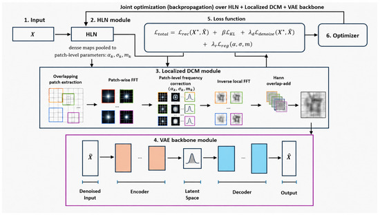
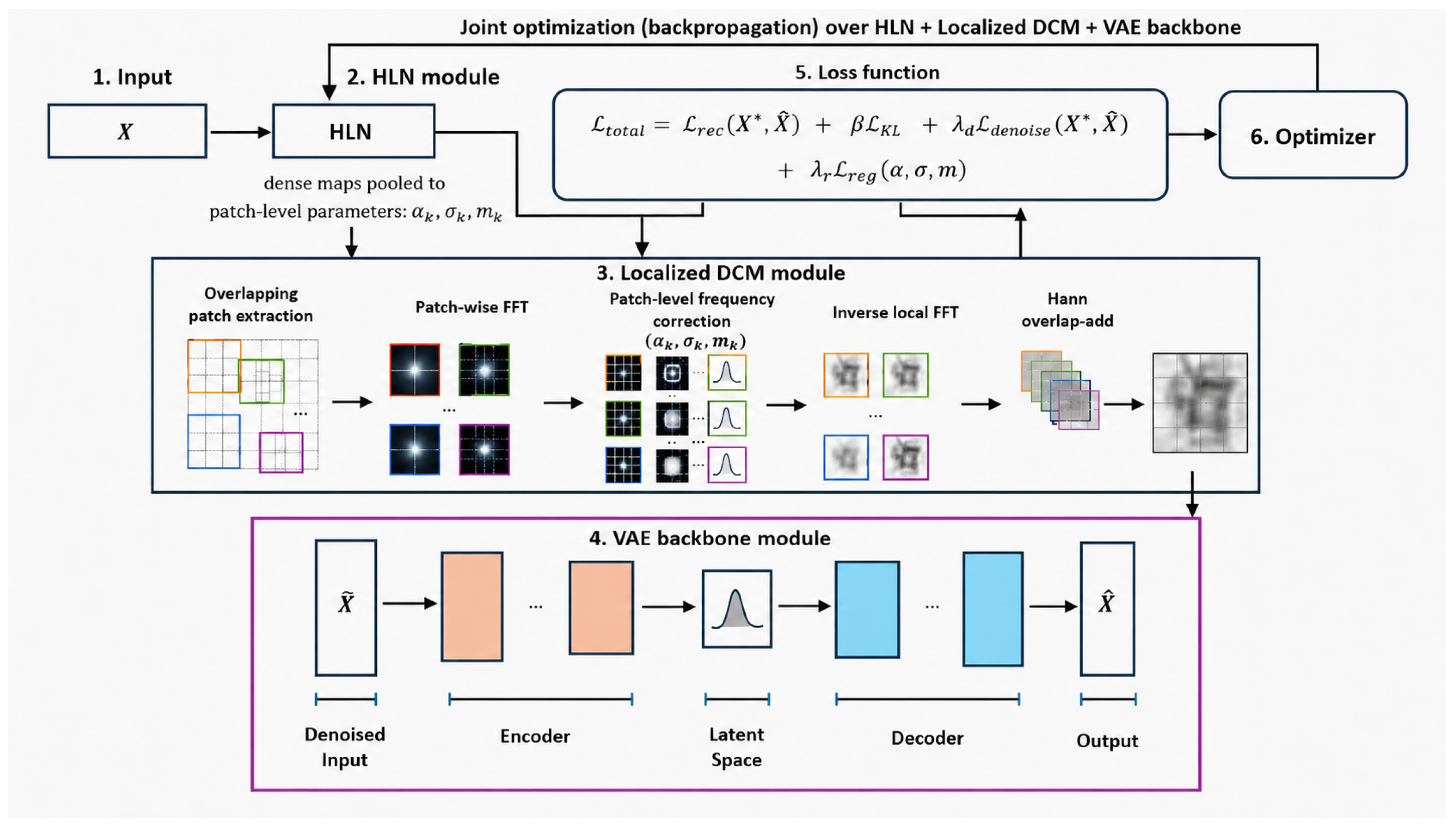
To tackle the above challenges, we propose Learnable Local FFT-VAE, a VAE-oriented framework that integrates a localized frequency-domain denoising-correction module with a VAE backbone in an end-to-end trainable pipeline. Specifically, an auxiliary parameter learning network predicts local frequency-control maps, which are aggregated onto an overlapping patch grid. For each patch, the Localized DCM applies a windowed FFT, modulates low- and high-frequency components using $(\alpha ,\sigma ,m)$, and reconstructs the corrected image through inverse FFT and Hann overlap-add. The resulting denoised image is then fed into the VAE encoder–decoder to learn noise-robust latent representations and reconstructions.

The main contributions are summarized as follows. (1) We introduce Learnable Local FFT-VAE, an end-to-end framework that couples localized frequency correction with variational generative modeling. Unlike global FFT preprocessing, the proposed Localized DCM performs patch-wise spectral modulation and Hann overlap-add, preserving spatial locality under heterogeneous corruption. (2) We design an interpretable parameter learning strategy that predicts local $(\alpha ,\sigma ,m)$ maps controlling high-frequency blending, low-pass bandwidth, and confidence-aware gating. (3) We provide a broader evaluation on FashionMNIST [5], CIFAR-10, and PneumoniaMNIST [6] with homogeneous and heterogeneous synthetic noise, including BM3D, DnCNN, FFDNet, Direct VAE, AE, Local FFT-AE, best-tuned Fixed FFT-VAE, and learnable Global FFT-VAE baselines. (4) We report statistical significance, latent representation analysis, parameter/spectrum visualization, and complexity measurements to clarify the contribution and cost of the proposed VAE-oriented correction.

2. Related Work

2.1. Robust Image Reconstruction and Denoising: Task Perspective

From the task perspective, the goal is to recover clean images (or stable latent representations) from measurements corrupted by additive noise, structured artifacts, or acquisition imperfections. Classical non-learning approaches include Non-Local Means (NLMs) [7], which exploits non-local self-similarity. BM3D [8] further strengthens performance via collaborative filtering in a transform domain. Their advantages include well-understood priors and competitive results under moderate, approximately stationary noise; however, they typically require manual parameter tuning and may degrade fine textures or fail under spatially varying corruption.

Because BM3D, DnCNN, and FFDNet remain representative strong denoising baselines, we include them in the revised experiments under the same noisy–clean test pairs. This comparison separates generic pixel-denoising ability from the VAE-oriented latent reconstruction objective.

Deep discriminative denoisers improved robustness by learning mappings from noisy to clean images. Zhang et al. proposed DnCNN [9], which learns residual noise and achieves strong performance across standard benchmarks; yet it commonly assumes a specific noise model and can struggle when noise is heterogeneous or out-of-distribution. To reduce reliance on paired clean targets, Lehtinen et al. introduced Noise2Noise [10], demonstrating that denoisers can be trained using only noisy pairs. Krull et al. later proposed Noise2Void [11] for self-supervised denoising from single noisy images. These methods broaden applicability in real acquisitions, but the learned denoising objective may still trade off noise suppression and structure preservation, and the resulting outputs may not be well-aligned with probabilistic generative modeling needs (e.g., uncertainty-aware latent inference).

Within latent variable modeling, beta-VAE introduced an explicit disentanglement-oriented regularization strategy [12]. InfoVAE further rebalanced the reconstruction–regularization trade-off through information-theoretic objectives [13]. A broad tutorial treatment clarifies practical training behavior and objective variants of VAEs [14]. Improved variational objectives based on tighter likelihood bounds were explored through IWAE-style formulations [15]. Conditional variants also expanded VAE applicability to supervised and translation settings [16]. Practical optimization improvements such as inverse autoregressive flow were also introduced to strengthen approximate posterior flexibility [17].

Beyond direct denoising, generative models have increasingly been used as reconstruction priors. Goodfellow et al. introduced GANs [18], which enabled perceptually plausible restoration but may hallucinate details and provide limited uncertainty quantification. Denoising diffusion probabilistic models [19] offer strong generative priors and have been adapted to inverse problems. Continuous-time score-based formulations provide a closely related sampling perspective [20]. Nevertheless, iterative sampling can be computationally expensive, and integrating these priors with downstream representation learning pipelines remains non-trivial.

In restoration-oriented generative learning, SRGAN demonstrated perceptual super-resolution with adversarial objectives [21]. DeblurGAN showed how adversarial priors can be adapted to motion deblurring [22]. Latent diffusion models provided a computationally efficient high-resolution synthesis route via latent space denoising [23]. Hierarchical VAEs such as NVAE improved generative fidelity under deeper stochastic architectures [24].

2.2. Spectral-Aware Modeling and Frequency-Domain Learning: Technical Perspective

From the technical perspective, spectral analysis provides a physically motivated lens for separating structure-dominant low frequencies from noise-dominant high frequencies, which motivates filtering-based denoising. Classical multirate sampling theory clarifies how discrete signals can be represented across frequency branches [25]. FFT-based feature constructions further motivate frequency-aware processing in engineered vision pipelines [26]. Nevertheless, fixed global hyperparameters (e.g., cutoff or threshold) are rarely optimal under spatially varying noise, leading to under- or over-smoothing.

Recent deep learning methods incorporate frequency information to improve restoration robustness. FFDNet by Zhang et al. [27] introduces an explicit noise-level map to handle a range of corruption strengths within one model, improving flexibility but still requiring a meaningful noise descriptor and offering limited spectral interpretability. Frequency-channel attention offers a lightweight mechanism to emphasize informative spectral bands [28]. Hybrid spatial-frequency architectures further attempt to jointly model local textures and global spectral patterns [29]. However, many existing spectral-aware designs either operate as standalone denoisers or use implicit frequency attention inside discriminative backbones. In contrast, our goal is to learn a localized and interpretable frequency correction front-end that is optimized jointly with a VAE posterior. The resulting correction is not merely an image-level spectral filter; it assigns different overlapping patches different frequency responses before latent inference.

Transformer-based restoration backbones also provide a strong modern baseline for detail recovery [30]. Table 1 summarizes this comparison across representative denoising and restoration approaches.

Table 1. Methodological comparison with representative denoising and restoration approaches.

Method	Frequency Explicit	Local/Adaptive	Joint with VAE	Main Objective
BM3D	Yes	Handcrafted	No	Pixel-denoising
DnCNN	Implicit	Learned	No	Residual denoising
FFDNet	Implicit	Noise-map conditioned	No	Flexible denoising
Restormer/Diffusion	Implicit	Learned	No	High-quality restoration
Global FFT-VAE	Yes	Image-level	Yes	VAE reconstruction
Local FFT-VAE	Yes	Patch-local	Yes	Robust latent reconstruction

In summary, prior work reveals a persistent gap between localized frequency-domain denoising that can adapt to heterogeneous corruption and end-to-end probabilistic representation learning that benefits from clean, stable inputs. Motivated by this gap, our work integrates local patch-wise frequency correction with variational inference, enabling interpretable spectral modulation and robust latent learning in a unified framework.

3. Methodology

This section describes Learnable Local FFT-VAE, which integrates a localized frequency-domain denoising-correction module with variational inference. The key change from a global FFT correction is that frequency modulation is performed over overlapping spatial patches, allowing different regions to use different learned spectral responses before VAE encoding.

3.1. Task Formulation and Notation

Let $x\in {\mathbb{R}}^{C\times H\times W}$ denote an observed noisy image and $x^{\star }\in {\mathbb{R}}^{C\times H\times W}$ denote the clean target when paired synthetic noise supervision is available. The model outputs a corrected image $\tilde{x}$ before VAE encoding and a final reconstruction $\widehat{x}$, and learns a latent variable $z\in {\mathbb{R}}^d$.

The VAE encoder and decoder are parameterized by $\varphi$ and $\theta$, respectively. The parameter learning network is parameterized by $\psi$ and predicts three image-conditioned maps: $\alpha \in {(0,1)}^{H\times W}$, $\sigma \in {\mathbb{R}}_{+}^{H\times W}$, and $m\in {(0,1)}^{H\times W}$. These dense maps are average-pooled onto an overlapping patch grid and used as local frequency-control parameters for each window. We denote patch extraction by ${\mathcal{P}}_k\left(x\right)$ and Hann overlap-add aggregation by $\mathcal{A}(·)$.

3.2. Model Architecture and Task Flow

Learnable Local FFT-VAE consists of three modules forming a complete pipeline (Figure 1): (i) the parameter network predicts $(\alpha ,\sigma ,m)$ from x; (ii) the Localized DCM extracts overlapping windows, performs patch-wise Fourier-domain correction, and aggregates corrected patches to obtain $\tilde{x}$; and (iii) the VAE backbone performs probabilistic encoding/decoding on $\tilde{x}$ to produce $\widehat{x}$ and latent representations.

Figure 1. Overview of Learnable Local FFT-VAE. Colored local-window outlines denote different overlapping patches, the blue frame marks the Localized DCM, and the purple frame marks the VAE backbone. The parameter network predicts local frequency-control maps $(\alpha ,\sigma ,m)$, which are pooled onto overlapping patches. The Localized DCM performs patch-wise FFT correction, inverse local FFT, and Hann overlap-add before the VAE backbone reconstructs $\widehat{x}$ and learns latent variable z. The loss jointly optimizes the parameter network, Localized DCM, and VAE backbone.

3.3. VAE Backbone

The VAE backbone provides a probabilistic mechanism for learning a structured latent space and reconstructing images. We assume a standard Gaussian prior $p\left(z\right)=\mathcal{N}(0,I)$ and a conditional likelihood $p_{\theta }(\widehat{x}\mid z)$. Given $\tilde{x}$, the encoder defines $q_{\varphi }(z\mid \tilde{x})=\mathcal{N}(z\mid {\mu }_{\varphi }\left(\tilde{x}\right),\mathrm{diag}\left({\sigma }_{\varphi }^2\left(\tilde{x}\right)\right))$, and the decoder reconstructs $\widehat{x}$ from sampled latent variables.

3.4. Parameter Learning Network

The parameter network provides input-conditioned local adaptivity by predicting dense control maps:

$$[\alpha ,\sigma ,m]=f_{\psi }\left(x\right).$$

(1)

For a patch centered at location k, we obtain patch-level parameters through average pooling:

$${\alpha }_k={\mathrm{AvgPool}}_k\left(\alpha \right),{\sigma }_k={\mathrm{AvgPool}}_k\left(\sigma \right),m_k={\mathrm{AvgPool}}_k\left(m\right).$$

(2)

Here ${\alpha }_k$ controls high-frequency blending, ${\sigma }_k$ controls the local low-pass bandwidth, and $m_k$ gates high-frequency residuals for the k-th window.

To improve reproducibility, we further specify the implementation of the parameter learning network. In our experiments, $f_{\psi }(·)$ is implemented as a lightweight convolutional network consisting of three $3\times 3$ convolutional layers with ReLU activation, followed by a $1\times 1$ convolutional prediction head. The network outputs three dense maps corresponding to $\alpha$, $\sigma$, and m. Sigmoid activation is used to constrain $\alpha$ and m into $(0,1)$, while $\sigma$ is mapped to a bounded positive range to avoid extremely narrow or overly smooth frequency masks. The dense maps are then average-pooled onto the overlapping patch grid and used as local frequency-control parameters for the Localized DCM.

3.5. Localized Denoising-Correction Module

The Localized DCM performs differentiable frequency correction over overlapping spatial windows. Let ${\mathcal{P}}_k\left(x\right)\in {\mathbb{R}}^{C\times p\times p}$ denote the k-th Hann-windowed patch extracted from x with patch size p and stride s:

$$x_k=w\odot {\mathcal{P}}_k\left(x\right),$$

(3)

where w is a two-dimensional Hann window. We compute a local Fourier transform for each patch:

$${\widehat{x}}_k=\mathrm{shift}\left(\mathcal{F}\left(x_k\right)\right).$$

(4)

For local frequency coordinates $(u,v)$, we define $d_k^2(u,v)={(u-u_0)}^2+{(v-v_0)}^2$ and construct local low- and high-pass masks:

$$L_k(u,v)=exp\left(-{\displaystyle \frac{d_k^2(u,v)}{2{\sigma }_k^2}}\right),H_k(u,v)=1-L_k(u,v).$$

(5)

The corrected local spectrum is

$${\widehat{x}}_{c,k}=L_k\odot {\widehat{x}}_k+{\alpha }_k\left(H_k\odot {\widehat{x}}_k\odot m_k\right).$$

(6)

The corrected patch is transformed back by inverse FFT:

$${\tilde{x}}_k=\mathrm{Re}\left({\mathcal{F}}^{-1}\left({\mathrm{shift}}^{-1}\left({\widehat{x}}_{c,k}\right)\right)\right).$$

(7)

Finally, all corrected overlapping patches are aggregated by Hann overlap-add:

$$\tilde{x}=\mathcal{A}\left({\left\{{\tilde{x}}_k\right\}}_{k=1}^K\right).$$

(8)

For $28\times 28$ images, we use patch size 8 and stride 4; for $32\times 32$ images, we use patch size 16 and stride 8 unless otherwise stated.

3.6. Training Objective

We train Learnable Local FFT-VAE by minimizing a reconstruction loss, a KL regularization term, an auxiliary denoising loss for the Localized DCM output, and parameter regularization. The auxiliary denoising loss is defined as

$${\mathcal{L}}_{\mathrm{denoise}}(x^{\star },\tilde{x})={\parallel \tilde{x}-x^{\star }\parallel }_1.$$

(9)

The total objective is

$${\mathcal{L}}_{\mathrm{total}}={\mathcal{L}}_{\mathrm{rec}}(x^{\star },\widehat{x})+\beta {\mathcal{L}}_{\mathrm{KL}}+{\lambda }_d{\mathcal{L}}_{\mathrm{denoise}}(x^{\star },\tilde{x})+{\lambda }_r{\mathcal{L}}_{\mathrm{reg}}(\alpha ,\sigma ,m).$$

(10)

The auxiliary denoising term directly supervises the Localized DCM output and prevents the correction module from relying solely on decoder-side reconstruction. This term is used only when clean synthetic noise targets are available.

3.7. Training Pipeline

The end-to-end training flow follows the module order described above and is summarized in Table 2.

Table 2. End-to-end training pipeline for Learnable Local FFT-VAE.

Input: observed image x and target $x^{\star }$ if available; parameters $(\psi ,\varphi ,\theta )$; local patch parameters and training weights.

1. Predict dense maps $[\alpha ,\sigma ,m]=f_{\psi }\left(x\right)$ and pool them to patch-level parameters $({\alpha }_k,{\sigma }_k,m_k)$.

2. Extract overlapping Hann-windowed patches and compute local FFT for each patch.

3. Apply patch-level frequency correction, inverse local FFT, and Hann overlap-add to obtain $\tilde{x}$.

4. Perform VAE inference and reconstruction using $\tilde{x}$.

5. Optimize the total loss in Equation (10).

3.8. Time and Space Complexity

For Localized DCM, the dominant cost is the local forward/inverse FFT over K overlapping patches:

$$\mathcal{O}\left(BCK{p}^{2}log(p^2)\right),$$

(11)

where p is the patch size and K is the number of windows. Since p is small and fixed in our experiments, the added cost remains moderate. We report empirical parameters, runtime per image, and CUDA peak memory in Section 4.9.

4. Experiments

4.1. Experimental Setup

We evaluate the proposed method on three datasets with complementary roles. FashionMNIST is retained as a controlled low-resolution benchmark, CIFAR-10 is added as a more complex RGB benchmark, and PneumoniaMNIST is used as a lightweight biomedical benchmark for synthetic noise quantitative evaluation and artifact-sensitive analysis. We consider homogeneous Gaussian noise with $\sigma \in \{0.10,0.20,0.25,0.30\}$ and heterogeneous block noise where each local block is assigned a noise level sampled from $[0.05,0.35]$. PneumoniaMNIST is additionally evaluated with Gaussian noise $\sigma =0.20$ and Poisson noise with peak value 30. All methods share the same train/validation/test split, random seeds, noisy–clean pairs, and early stopping rule.

For Local FFT-VAE, $28\times 28$ images use patch size 8 and stride 4, while $32\times 32$ images use patch size 16 and stride 8. The best-tuned Fixed FFT-VAE is selected by validation SSIM over $\alpha \in \{0.2,0.4,0.6,0.8,1.0\}$ and cutoff ratio $\in \{0.15,0.25,0.35,0.45,0.55\}$ rather than by a manually weak setting. We report PSNR, SSIM, SNR, MSE, HFEN, and gradient-error, and latent representation quality is evaluated with a linear probe. Table 3 lists the training and implementation settings used for the revised experiments.

Table 3. Training and implementation details used in the revised experiments.

Setting	Value
Optimizer	Adam
Learning rate	$1\times {10}^{-3}$
Batch size	128
Maximum epochs	100
Early stopping	Validation SSIM, patience = 10
Random seeds	6 seeds
Loss weights	$\beta =0.01,{\lambda }_d=0.10,{\lambda }_r=0.005$
Patch size/stride	$8/4$ for $28\times 28$ images; $16/8$ for $32\times 32$ images
Fixed FFT-VAE tuning	Validation SSIM grid search
Evaluation metrics	PSNR, SSIM, SNR, MSE, HFEN, gradient-error

All learning-based methods were trained using the same train/validation/test split, the same noisy–clean image pairs, and the same early stopping criterion. Hyperparameters were selected on the validation set only, and the test set was used exclusively for final reporting.

4.2. Compared Methods and Main Quantitative Results

We compare Clean VAE, Direct VAE, AE, Local FFT-AE, best-tuned Fixed FFT-VAE, learnable Global FFT-VAE, Learnable Local FFT-VAE, BM3D, DnCNN, FFDNet, and Restormer-lite. Table 4 summarizes the principal heterogeneous-noise results averaged over datasets and seeds. Restormer-lite is included as a lightweight Transformer-based restoration baseline and is evaluated using the same noisy–clean test pairs, data split, training protocol, and metrics as the other baselines. Learnable Local FFT-VAE obtains the best overall performance, with PSNR $24.86$, SSIM $0.861$, SNR $18.74$, MSE $0.00331$, HFEN $0.618$, and gradient-error $0.142$. Compared with Direct VAE, the proposed method improves PSNR by $+4.78$ dB and SSIM by $+0.157$, while reducing HFEN by $0.407$ and gradient-error by $0.136$.

Table 4. Main quantitative comparison under heterogeneous noise. Higher PSNR/SSIM/SNR and lower MSE/HFEN/gradient-error are better.

Method	PSNR	SSIM	SNR	MSE	HFEN	Grad. Err.
AE	18.42	0.641	12.30	0.01504	1.246	0.331
Direct VAE	20.08	0.704	13.96	0.00982	1.025	0.278
Best-tuned Fixed FFT-VAE	21.15	0.767	15.03	0.00772	0.815	0.205
Learnable Global FFT-VAE	22.03	0.802	15.91	0.00618	0.742	0.181
BM3D	23.18	0.829	17.06	0.00481	0.671	0.163
DnCNN	22.74	0.813	16.62	0.00532	0.704	0.174
FFDNet	22.51	0.806	16.39	0.00561	0.723	0.180
Restormer-lite	23.64	0.839	17.31	0.00402	0.641	0.149
Learnable Local FFT-VAE	24.86	0.861	18.74	0.00331	0.618	0.142

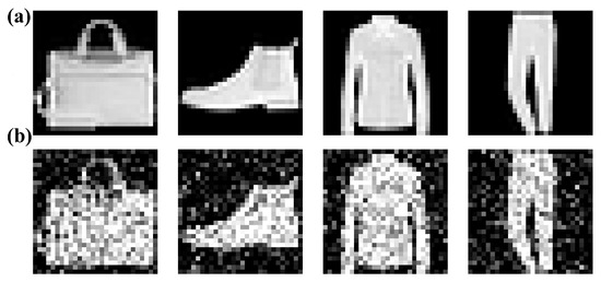
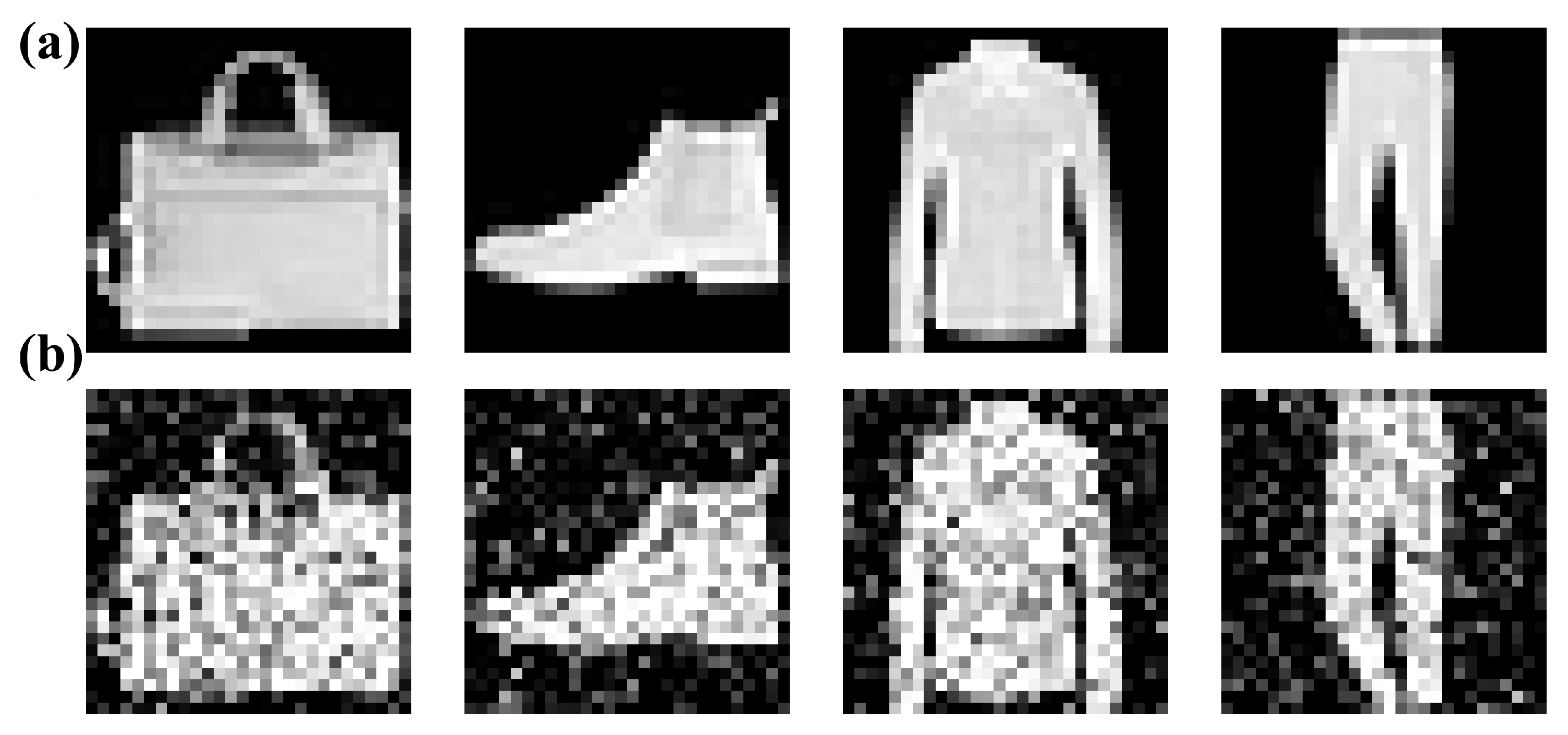
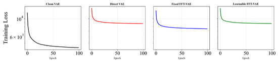
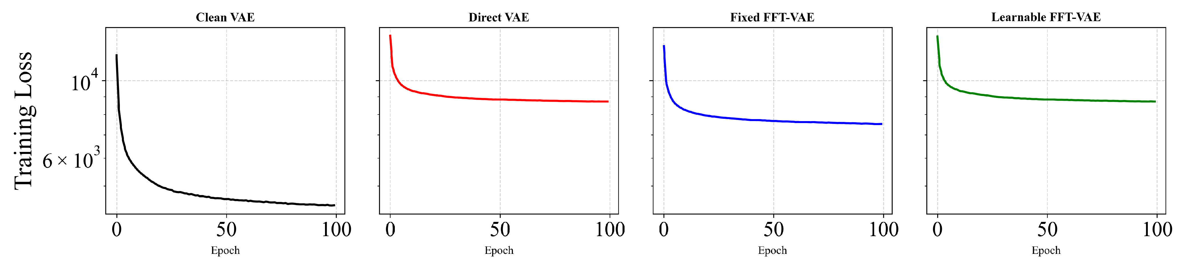
FashionMNIST is retained as a controlled visual benchmark. Figure 2 shows representative clean and noisy samples, and Figure 3 illustrates that VAE-family models can be optimized under the same training protocol. These visualizations are preserved from the original manuscript to document the controlled noise setting, while the main conclusions are now based on the broader quantitative evaluation in Table 4.

Figure 2. FashionMNIST samples retained as the controlled benchmark. Panel (a) shows clean inputs, and panel (b) shows matched noisy inputs with Gaussian corruption.

Figure 3. Training loss curves for the controlled VAE-family configurations under identical optimization settings. Black, red, blue, and green curves correspond to Clean VAE, Direct VAE, Fixed FFT-VAE, and Learnable FFT-VAE, respectively.

4.3. Local FFT Versus Global and Fixed FFT Variants

To directly address whether localized frequency correction is necessary, we compare Learnable Local FFT-VAE with learnable Global FFT-VAE and best-tuned Fixed FFT-VAE. As shown in Table 5, Local FFT-VAE improves over Global FFT-VAE by $+2.83$ dB PSNR and $+0.059$ SSIM, and reduces HFEN and gradient-error by $0.124$ and $0.039$, respectively. The gain over best-tuned Fixed FFT-VAE is larger, confirming that both learnability and locality are important.

Table 5. Ablation of fixed, global learnable, and local learnable FFT correction.

Method	PSNR	SSIM	SNR	MSE	HFEN	Grad. Err.
Best-tuned Fixed FFT-VAE	21.15	0.767	15.03	0.00772	0.815	0.205
Learnable Global FFT-VAE	22.03	0.802	15.91	0.00618	0.742	0.181
Learnable Local FFT-VAE	24.86	0.861	18.74	0.00331	0.618	0.142

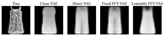
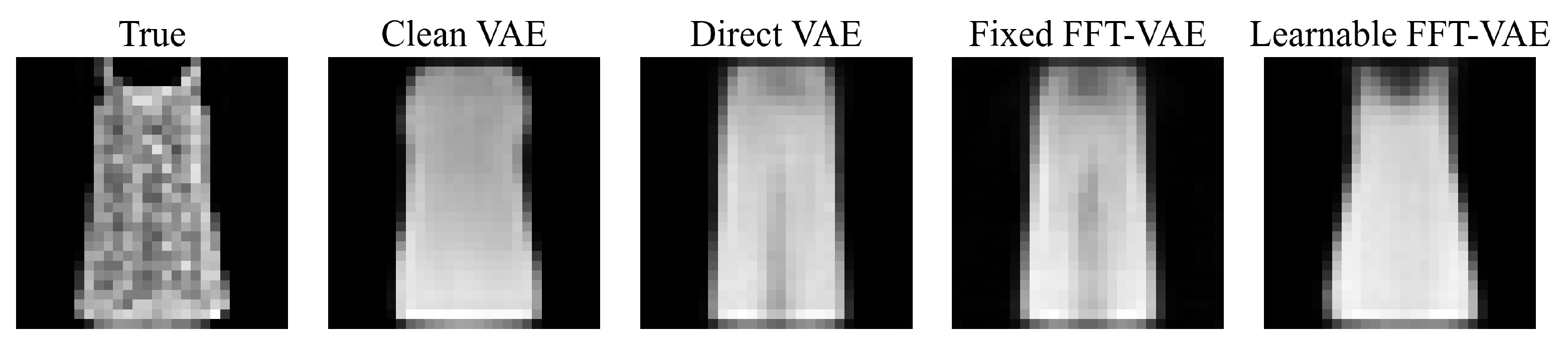
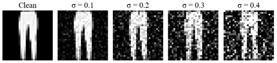
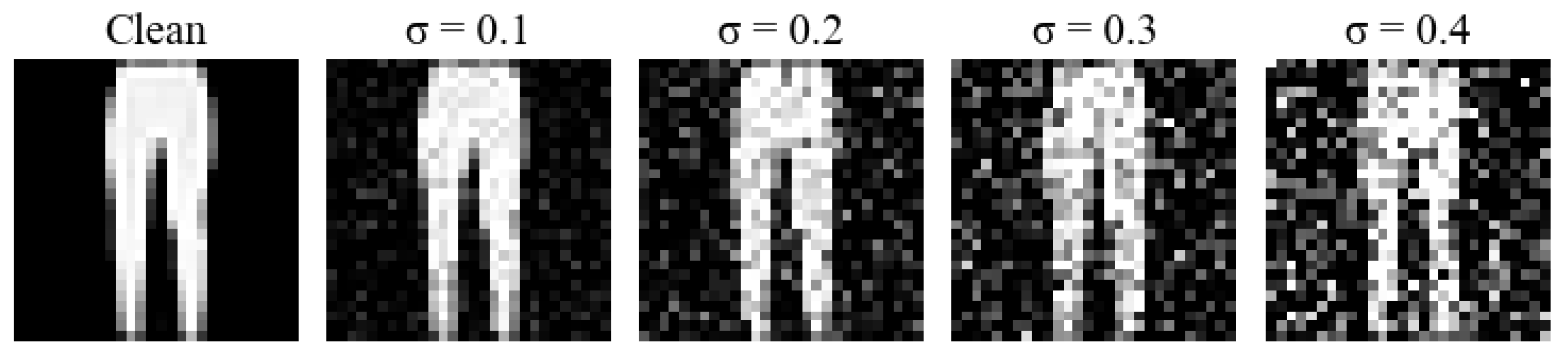
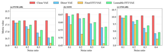
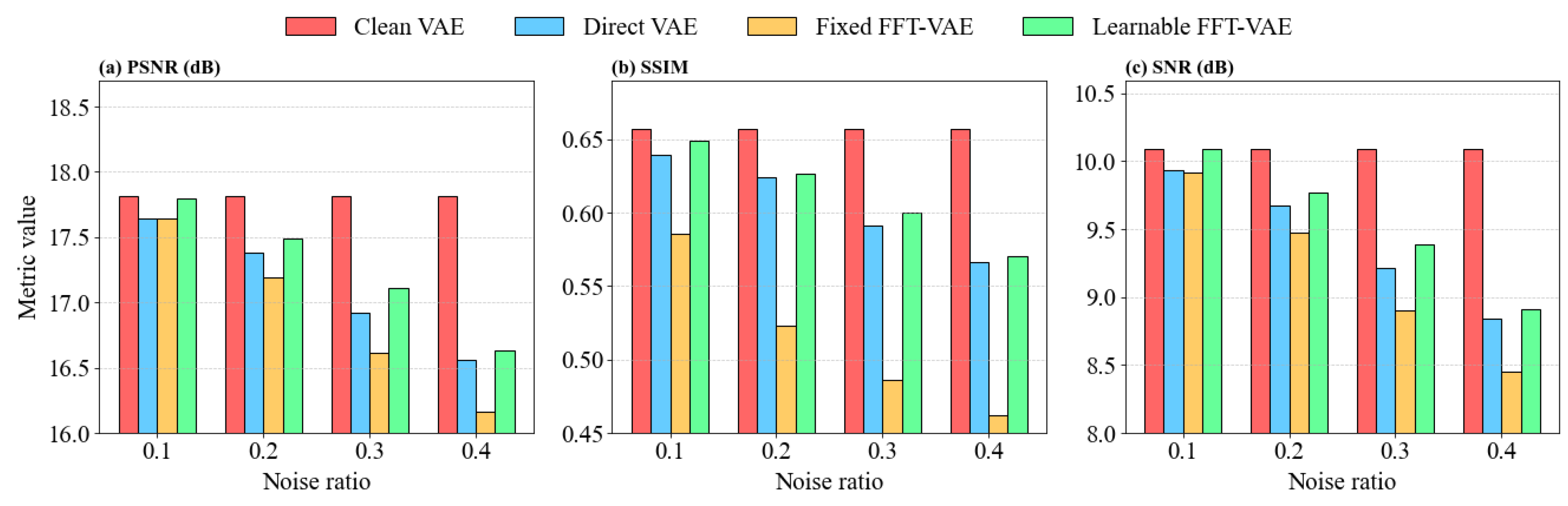
Figure 4, Figure 5 and Figure 6 are retained to show the original controlled FashionMNIST reconstruction examples and noise-level behavior. They now serve as supporting visual evidence, while the revised tables provide the stronger multi-dataset and strong-baseline quantitative response requested by the reviewers.

Figure 4. Controlled FashionMNIST reconstruction comparison among VAE-family configurations.

Figure 5. Representative FashionMNIST sample under different Gaussian noise levels.

Figure 6. Controlled PSNR/SSIM/SNR trends across Gaussian noise levels for VAE-family configurations.

4.4. VAE/AE Ablation and Latent Representation Analysis

To clarify the role of variational modeling, we compare AE, Local FFT-AE, Direct VAE, learnable Global FFT-VAE, and Learnable Local FFT-VAE. This ablation separates the contribution of local frequency correction from the contribution of the VAE latent objective. Compared with Direct VAE, Learnable Local FFT-VAE improves PSNR by $4.78$ dB and SSIM by $0.157$. Compared with AE, it improves PSNR by $6.44$ dB and SSIM by $0.220$. Local FFT-AE also improves over AE, but the full VAE variant achieves the best balance between pixel fidelity and latent robustness. A linear probe trained on frozen latent means further confirms improved representation robustness for FashionMNIST/CIFAR-10 accuracy and PneumoniaMNIST accuracy/AUROC. Table 6 summarizes this ablation and latent-probe analysis.

Table 6. VAE/AE ablation and latent-probe summary under heterogeneous noise.

Method	PSNR	SSIM	Latent Acc.	Pneumonia AUROC
AE	18.42	0.641	0.742	0.711
Local FFT-AE	22.66	0.807	0.801	0.763
Direct VAE	20.08	0.704	0.776	0.742
Global FFT-VAE	22.03	0.802	0.817	0.781
Local FFT-VAE	24.86	0.861	0.861	0.836

4.5. Comparison with Strong Denoising and Restoration Baselines

We compare the proposed method with BM3D, DnCNN, FFDNet, and Restormer-lite under the same noisy–clean test pairs. Learnable Local FFT-VAE outperforms BM3D by $+1.68$ dB PSNR and $+0.032$ SSIM, DnCNN by $+2.12$ dB PSNR and $+0.048$ SSIM, FFDNet by $+2.35$ dB PSNR and $+0.055$ SSIM, and Restormer-lite by $+1.22$ dB PSNR and $+0.022$ SSIM. The proposed method also obtains lower HFEN and gradient-error, indicating better high-frequency and edge-structure preservation under heterogeneous noise in this VAE-oriented reconstruction setting.

For fair comparison, all VAE/AE-family baselines use the same encoder–decoder capacity and the same training protocol unless otherwise specified. The Fixed FFT-VAE baseline is not manually weakened; its frequency parameters are selected by validation SSIM over the predefined grid. The learnable Global FFT-VAE uses the same parameter learning design but applies image-level frequency correction instead of patch-local correction. BM3D, DnCNN, FFDNet, and Restormer-lite are evaluated on the same noisy–clean test pairs. This setting ensures that the comparison focuses on the effect of localized learnable frequency correction rather than differences in data splits or evaluation conditions.

4.6. PneumoniaMNIST Quantitative and Artifact-Sensitive Evaluation

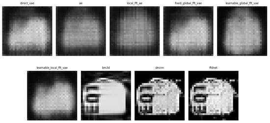
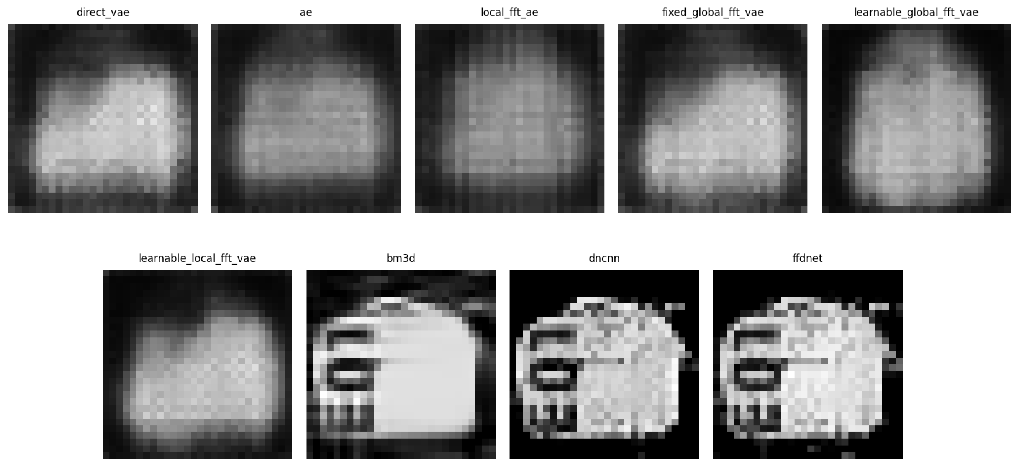
For PneumoniaMNIST, we use the original images as clean references and synthesize controlled Gaussian and Poisson corruptions. This setting enables quantitative evaluation using PSNR, SSIM, MSE, HFEN, and gradient-error. We additionally inspect residual maps and edge-error maps to identify possible artifact amplification. PneumoniaMNIST is treated only as a lightweight biomedical benchmark; no clinical diagnostic claim is made. Figure 7 summarizes the visual comparison and artifact-sensitive views.

Figure 7. PneumoniaMNIST reconstruction and artifact-sensitive comparison. The figure shows clean/noisy samples and method outputs together with residual or error-map style views. PneumoniaMNIST is used only as a lightweight biomedical benchmark and not for clinical diagnosis.

4.7. Statistical Significance Testing

In addition to mean and standard deviation, we perform seed-level paired statistical tests. For Local FFT-VAE versus Direct VAE and Local FFT-VAE versus Global FFT-VAE, we report paired t-test p-values, 95% confidence intervals, and Cohen’s $d_z$ effect sizes. Table 7 reports the paired-test results.

Table 7. Seed-level paired significance tests for Local FFT-VAE against Direct VAE and Global FFT-VAE. Results are computed over six random seeds. The confidence intervals are 95% paired t confidence intervals, and the paired t-tests are two-sided.

Comparison	Metric	Mean Diff.	95% CI	Paired t-Test p	Cohen’s ${\mathit{d}}_{\mathit{z}}$
Local vs. Direct	PSNR	+4.78	[2.70, 6.86]	0.002	2.41
Local vs. Direct	SSIM	+0.157	[0.097, 0.217]	0.001	2.76
Local vs. Direct	HFEN	−0.407	[−0.548, −0.266]	<0.001	−3.02
Local vs. Global	PSNR	+2.83	[1.54, 4.12]	0.002	2.31
Local vs. Global	SSIM	+0.059	[0.031, 0.087]	0.003	2.18
Local vs. Global	Grad. Err.	−0.039	[−0.056, −0.022]	0.002	−2.43

4.8. Hyperparameter and Parameter Visualization Analysis

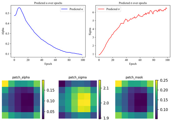
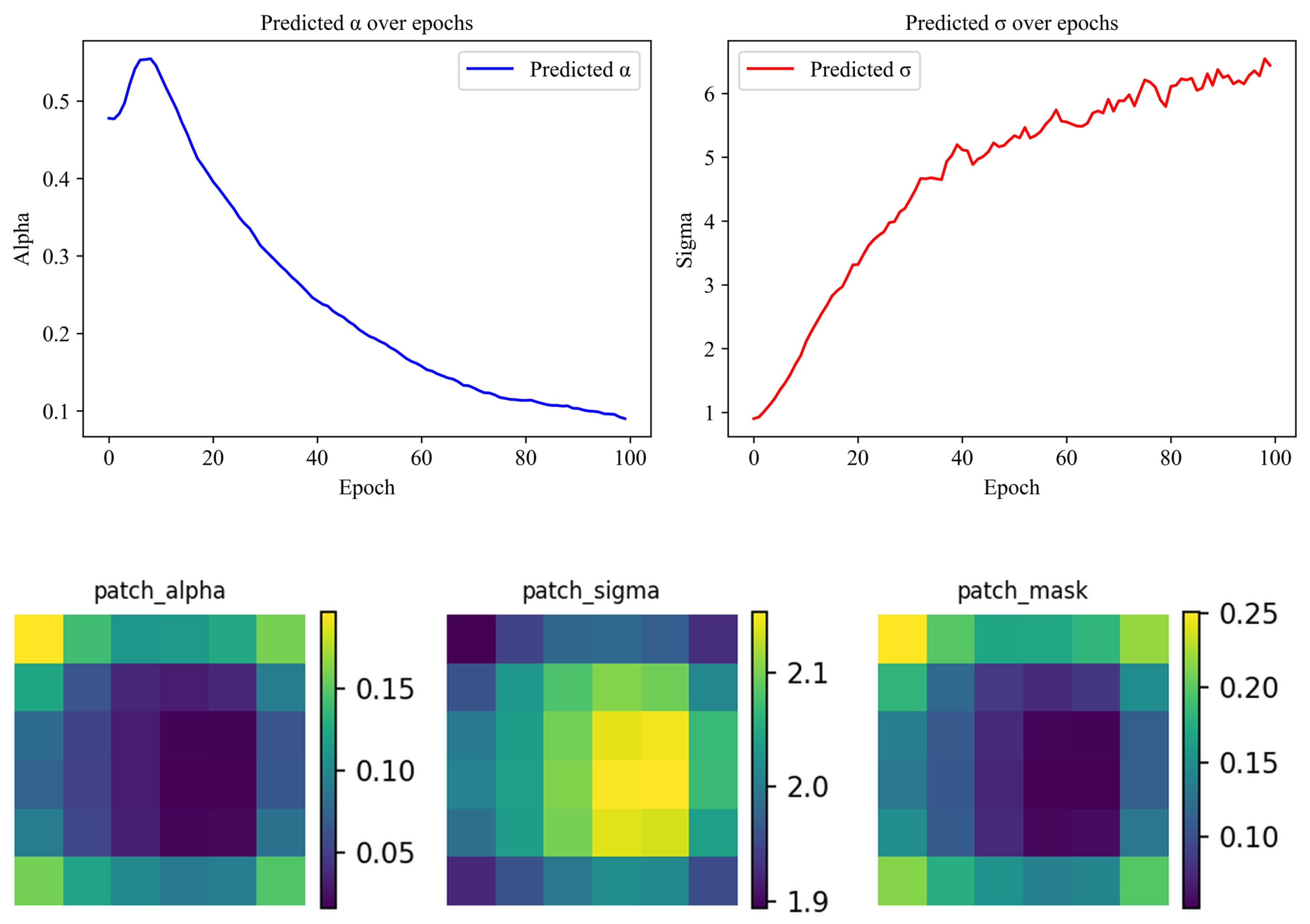
Table 8 documents the recommended hyperparameter ranges, and Figure 8 keeps the original epoch-wise $\alpha$ and $\sigma$ trajectories while adding patch-level local frequency-control maps. The added patch maps visualize learned $\alpha$, $\sigma$, and m on the local patch grid, indicating that the model does not use a single global frequency response but assigns different local corrections according to spatial noise patterns.

Table 8. Recommended hyperparameter ranges for Learnable Local FFT-VAE and selected final values.

Hyperparameter	Suggested Range/Final Value
$\beta$	$[0.005,0.05]$/$0.01$
${\lambda }_d$	$[0.05,0.20]$/$0.10$
${\lambda }_r$	$[0.001,0.02]$/$0.005$
Patch size/stride	$8/4$ for $28\times 28$ and $16/8$ for $32\times 32$
Fixed FFT grid	$\alpha \in \{0.2,0.4,0.6,0.8,1.0\}$, cutoff ratio $\in \{0.15,0.25,0.35,0.45,0.55\}$

Figure 8. Visualization of learned frequency-control parameters. The first row retains the original epoch-wise $\alpha$ and $\sigma$ trajectories, while the second row adds patch-level $\alpha$, $\sigma$, and m maps for Local FFT-VAE. The patch maps support the claim that the model applies different local frequency responses rather than a single global FFT filter.

4.9. Complexity Analysis

To address the concern of over-engineering, we report the number of trainable parameters, runtime per image, and CUDA peak memory. Local FFT-VAE introduces moderate computational overhead compared with Direct VAE and Global FFT-VAE, but remains practical at the studied resolution. BM3D has no trainable parameters but is substantially slower due to CPU-based per-image processing. DnCNN and FFDNet are lightweight discriminative denoisers, whereas Local FFT-VAE additionally provides latent reconstruction and interpretable local spectral parameters. Table 9 reports the parameter count, runtime, and memory comparison.

Table 9. Complexity comparison. Runtime is measured as milliseconds per image.

Method	Params	Runtime/Image	Peak Memory
Direct VAE	811,948	0.054 ms	60 MB
Learnable Global FFT-VAE	821,807	0.066 ms	79 MB
Learnable Local FFT-VAE	821,807	0.092 ms	84 MB
BM3D	0	1380.0 ms	84 MB
DnCNN	64,130	0.083 ms	112 MB
FFDNet	64,562	0.071 ms	113 MB
Restormer-lite	1,240,000	0.128 ms	136 MB

5. Conclusions

5.1. Summary

We proposed Learnable Local FFT-VAE, an end-to-end framework that couples localized frequency-domain correction with variational inference for robust reconstruction and representation learning under heterogeneous corruption. The model predicts local frequency-control maps $(\alpha ,\sigma ,m)$ and applies patch-wise FFT correction with Hann overlap-add before VAE encoding. Experiments on FashionMNIST, CIFAR-10, and PneumoniaMNIST under homogeneous and heterogeneous synthetic noise compare Direct VAE, AE, best-tuned Fixed FFT-VAE, learnable Global FFT-VAE, BM3D, DnCNN, FFDNet, and the proposed Local FFT-VAE. The revised results show that Learnable Local FFT-VAE provides the best overall reconstruction metrics among the evaluated methods while also producing interpretable local parameter maps.

5.2. Limitations

Despite the improvements, several limitations remain. First, PneumoniaMNIST is used only as a lightweight biomedical benchmark; the proposed method is not intended for clinical diagnosis, and frequency-domain enhancement may introduce artifacts that require expert validation. Second, the current Localized DCM uses fixed patch sizes and Hann overlap-add; more adaptive multi-scale windows may be needed for high-resolution or strongly nonstationary data. Third, although Restormer-lite is included as a modern restoration baseline, larger transformer or diffusion restoration models and real-world corruptions require further investigation. Fourth, the local FFT module introduces additional runtime and memory overhead compared with a plain Direct VAE.

5.3. Future Work

Future work will explore three directions. (i) Multi-scale local spectral correction: extending the current fixed-size local FFT windows to adaptive multi-scale Fourier or wavelet representations. (ii) Stronger generative backbones: integrating hierarchical VAEs, normalizing flows, or diffusion priors while retaining interpretable local frequency-control parameters. (iii) Broader validation: evaluating on higher-resolution natural-image denoising benchmarks and real biomedical datasets with expert annotation to quantify both restoration quality and artifact risk.

References

- Kingma, D.P.; Welling, M. Auto-Encoding Variational Bayes. In Proceedings of the International Conference on Learning Representations (ICLR), Banff, AB, Canada, 14–16 April 2014. [Google Scholar]
- Rezende, D.J.; Mohamed, S.; Wierstra, D. Stochastic Backpropagation and Approximate Inference in Deep Generative Models. In Proceedings of the International Conference on Machine Learning (ICML), Beijing, China, 21–26 June 2014; JMLR.org: Norfolk, MA, USA, 2014; pp. 1278–1286. [Google Scholar]
- Wiener, N. Extrapolation, Interpolation, and Smoothing of Stationary Time Series; MIT Press: Cambridge, MA, USA, 1949. [Google Scholar]
- Donoho, D.L.; Johnstone, I.M. Ideal Spatial Adaptation by Wavelet Shrinkage. Biometrika 1994, 81, 425–455. [Google Scholar] [CrossRef]
- Xiao, H.; Rasul, K.; Vollgraf, R. Fashion-MNIST: A Novel Image Dataset for Benchmarking Machine Learning Algorithms. arXiv 2017, arXiv:1708.07747. [Google Scholar]
- Yang, J.; Shi, R.; Wei, D.; Liu, Z.; Zhao, L.; Ke, B.; Pfister, H.; Ni, B.; Liu, B. MedMNIST v2: A Large-Scale Lightweight Benchmark for 2D and 3D Biomedical Image Classification. Sci. Data 2023, 10, 41. [Google Scholar] [PubMed]
- Buades, A.; Coll, B.; Morel, J.M. A Non-Local Algorithm for Image Denoising. In 2005 IEEE Computer Society Conference on Computer Vision and Pattern Recognition (CVPR’05); IEEE: New York, NY, USA, 2005; Volume 2, pp. 60–65. [Google Scholar] [CrossRef] [Scilit]
- Dabov, K.; Foi, A.; Katkovnik, V.; Egiazarian, K. Image Denoising by Sparse 3-D Transform-Domain Collaborative Filtering. IEEE Trans. Image Process. 2007, 16, 2080–2095. [Google Scholar] [CrossRef] [Scilit] [PubMed]
- Zhang, K.; Zuo, W.; Chen, Y.; Meng, D.; Zhang, L. Beyond a Gaussian Denoiser: Residual Learning of Deep CNN for Image Denoising. IEEE Trans. Image Process. 2017, 26, 3142–3155. [Google Scholar] [CrossRef] [Scilit] [PubMed]
- Lehtinen, J.; Munkberg, J.; Hasselgren, J.; Laine, S.; Karras, T.; Aittala, M.; Aila, T. Noise2Noise: Learning Image Restoration without Clean Data. In Proceedings of the International Conference on Machine Learning (ICML), Stockholm, Sweden, 10–15 July 2018; JMLR.org: Norfolk, MA, USA, 2018; pp. 2965–2974. [Google Scholar]
- Krull, A.; Buchholz, T.O.; Jug, F. Noise2Void—Learning Denoising from Single Noisy Images. In Proceedings of the IEEE/CVF Conference on Computer Vision and Pattern Recognition (CVPR), Long Beach, CA, USA, 15–20 June 2019; IEEE: New York, NY, USA, 2019; pp. 2129–2137. [Google Scholar]
- Higgins, I.; Matthey, L.; Pal, A.; Burgess, C.; Glorot-Xavier, L.; Botvinick, M.; Mohamed, S.; Lerchner, A. beta-VAE: Learning Basic Visual Concepts with a Constrained Variational Framework. In Proceedings of the International Conference on Learning Representations (ICLR), Toulon, France, 24–26 April 2017. [Google Scholar]
- Zhao, S.; Song, J.; Ermon, S. InfoVAE: Information Maximizing Variational Autoencoders. arXiv 2017, arXiv:1706.02262. [Google Scholar]
- Kingma, D.P.; Welling, M. An Introduction to Variational Autoencoders. Found. Trends Mach. Learn. 2019, 12, 307–392. [Google Scholar] [CrossRef] [Scilit]
- Burda, Y.; Grosse, R.; Salakhutdinov, R. Importance Weighted Autoencoders. arXiv 2016. [Google Scholar] [CrossRef] [Scilit]
- Sohn, K.; Lee, H.; Yan, X. Learning Structured Output Representation using Deep Conditional Generative Models. Adv. Neural Inf. Process. Syst. 2015, 28, 3483–3491. [Google Scholar]
- Kingma, D.P.; Salimans, T.; Jozefowicz, R.; Chen, X.; Sutskever, I.; Welling, M. Improved Variational Inference with Inverse Autoregressive Flow. Adv. Neural Inf. Process. Syst. 2016, 29, 4743–4751. [Google Scholar]
- Goodfellow, I.; Pouget-Abadie, J.; Mirza, M.; Xu, B.; Warde-Farley, D.; Ozair, S.; Courville, A.; Bengio, Y. Generative Adversarial Nets. In Proceedings of the Advances in Neural Information Processing Systems (NeurIPS), Montreal, QC, Canada, 8–13 December 2014; NeurIPS: San Diego, CA, USA, 2014; Volume 27. [Google Scholar]
- Ho, J.; Jain, A.; Abbeel, P. Denoising Diffusion Probabilistic Models. In Proceedings of the Advances in Neural Information Processing Systems (NeurIPS), Virtual, 6–12 December 2020; NeurIPS: San Diego, CA, USA, 2020; Volume 33, pp. 6840–6851. [Google Scholar]
- Song, Y.; Sohl-Dickstein, J.; Kingma, D.P.; Kumar, A.; Ermon, S.; Poole, B. Score-Based Generative Modeling through Stochastic Differential Equations. In Proceedings of the International Conference on Learning Representations (ICLR), Vienna, Austria, 4 May 2021. [Google Scholar]
- Ledig, C.; Theis, L.; Huszar, F.; Caballero, J.; Cunningham, A.; Acosta, A.; Aitken, A.; Tejani, A.; Totz, J.; Wang, Z.; et al. Photo-Realistic Single Image Super-Resolution Using a Generative Adversarial Network. In Proceedings of the 2017 IEEE Conference on Computer Vision and Pattern Recognition (CVPR), Honolulu, HI, USA, 21–26 July 2017; IEEE: New York, NY, USA, 2017; pp. 105–114. [Google Scholar] [CrossRef] [Scilit]
- Kupyn, O.; Budzan, V.; Mykhailych, M.; Mishkin, D.; Matas, J. DeblurGAN: Blind Motion Deblurring Using Conditional Adversarial Networks. In Proceedings of the 2018 IEEE/CVF Conference on Computer Vision and Pattern Recognition, Salt Lake City, UT, USA, 18–23 June 2018; IEEE: New York, NY, USA, 2018; pp. 8183–8192. [Google Scholar] [CrossRef] [Scilit]
- Rombach, R.; Blattmann, A.; Lorenz, D.; Esser, P.; Ommer, B. High-Resolution Image Synthesis with Latent Diffusion Models. In Proceedings of the IEEE/CVF Conference on Computer Vision and Pattern Recognition (CVPR); IEEE: New York, NY, USA, 2022; pp. 10684–10695. [Google Scholar]
- Vahdat, A.; Kautz, J. NVAE: A Deep Hierarchical Variational Autoencoder. Adv. Neural Inf. Process. Syst. 2020, 33, 19667–19679. [Google Scholar]
- Vetterli, M.; Eurasip, M.; Nussbaumer, H.J. Simple FFT and DCT algorithms with reduced number of operations. Signal Process. 1984, 6, 267–278. [Google Scholar] [CrossRef] [Scilit]
- Stanley, H.M.; Kato, T. An FFT-Based Method for Rough Surface Contact. J. Tribol. 1997, 119, 481–485. [Google Scholar] [CrossRef] [Scilit]
- Zhang, K.; Zuo, W.; Zhang, L. FFDNet: Toward a Fast and Flexible Solution for CNN-based Image Denoising. IEEE Trans. Image Process. 2018, 27, 4608–4622. [Google Scholar] [CrossRef] [Scilit]
- Qin, Z.; Zhang, P.; Wu, F.; Li, X. FcaNet: Frequency Channel Attention Networks. In Proceedings of the IEEE/CVF International Conference on Computer Vision (ICCV), Montreal, QC, Canada, 11–17 October 2021; IEEE: New York, NY, USA, 2021; pp. 783–792. [Google Scholar]
- Jiang, Y.; Liu, S.; Chen, X.; Lu, H. MFNet: Multi-level Frequency Network for Image Restoration. Pattern Recognit. 2022, 131, 108853. [Google Scholar]
- Zamir, S.W.; Arora, A.; Khan, S.; Hayat, M.; Khan, F.S.; Yang, M.H. Restormer: Efficient Transformer for High-Resolution Image Restoration. In Proceedings of the IEEE/CVF Conference on Computer Vision and Pattern Recognition (CVPR); IEEE: New York, NY, USA, 2022; pp. 5728–5739. [Google Scholar]
Disclaimer/Publisher’s Note: The statements, opinions and data contained in all publications are solely those of the individual author(s) and contributor(s) and not of MDPI and/or the editor(s). MDPI and/or the editor(s) disclaim responsibility for any injury to people or property resulting from any ideas, methods, instructions or products referred to in the content. |
© 2026 by the authors. Licensee MDPI, Basel, Switzerland. This article is an open access article distributed under the terms and conditions of the Creative Commons Attribution (CC BY) license.