Condensed-History GPU Positron Range Simulator in Heterogeneous Media for PET Resolution Modelling

Featured Application

GPU-accelerated and condensed-history Monte Carlo computation of 3D positron annihilation images for tissue-dependent image reconstruction in clinical PET imaging.

Abstract

Positron range (PR) degrades spatial resolution in positron emission tomography (PET), with its effect being radionuclide- and medium-dependent. Current accurate PR simulators are computationally intensive and cannot be used in clinical time frames. This work presents the Hybrid Monte Carlo (HMC) PR simulator, a GPU-accelerated condensed-history code in CUDA Fortran for 3D annihilation imaging in heterogeneous voxelised geometries derived from CT images and $\mu$-maps. Pre-computed look-up interaction tables (LUTs) covering 24 reference-tissue materials and support for arbitrary ${\beta }^{+}$ emitters up to 3.55 MeV end-point energies (⁶⁸Ga, ⁸²Rb, ¹²⁴I, etc.) allow both GPU and CPU implementations. Maximum speeds reach $4.77·{10}^5$ (Intel i9-14900KF) and $3.32·{10}^8$ (NVIDIA RTX 5080) histories/s, surpassing prior CPU-only PenEasy 2024 by up to 4 orders of magnitude. A fixed step of 0.5 mm was chosen for LUT generation with a uniform $\pm 10\%$ variation each HMC step that allowed reducing aliasing effects. These values are consistent with our previous cross-code benchmark for the isotopes studied. Close agreement with PenEasy 2024 is demonstrated: point-source FWHM and FWTM residuals using ¹⁸F, ⁶⁸Ga, ¹²⁴I and ⁸²Rb are below 0.3 mm at ${10}^7$ histories, and voxelwise $R^2=0.995$, $\mathrm{SSIM}=0.995$ and PSNR $\approx 36.4$ dB are achieved simulating ⁸²Rb uptake from a human-scale [¹⁸F]FDG myocardium acquisition, while decreasing the simulation time from almost 9 h to roughly 1 s using HMC GPU. The resulting annihilation maps enable PET resolution modelling and patient-specific PR correction within clinically practical time frames.

1. Introduction

Positron emission tomography (PET) is a non-invasive molecular imaging technique that provides functional information about biological processes in vivo [1]. The spatial resolution achieved by modern PET scanners depends on several detector-dependent factors, including crystal size, depth of interaction, and detection efficiency. However, there is also a fundamental detector-independent contribution to resolution degradation: the finite distance travelled by the positron from its emission point to the site of annihilation. This phenomenon, commonly referred to as positron range (PR), introduces a non-trivial blurring that depends on the kinetic energy of the emitted positron, the density and composition of the surrounding tissue, and the presence of heterogeneous anatomical interfaces [1,2,3]. Conti and Eriksson have provided a comprehensive review of the physics of pure and non-pure positron emitters relevant to PET imaging [4].

The degree of resolution degradation associated with PR varies considerably across radionuclides. For ¹⁸F, the most commonly used PET isotope in clinical practice in the form of [¹⁸F]-FDG for glucose metabolism studies, the maximum positron energy is $Q=633.5$ keV, and the resulting range in water is relatively small (FWHM < 1 mm). However, other radionuclides with increasing clinical relevance emit positrons with substantially higher energies, leading to larger ranges that can significantly degrade image quality [5,6]. In particular, ⁶⁸Ga ($Q=1899$ keV) has become widely used for neuroendocrine tumour imaging with somatostatin analogues and for prostate cancer assessment with PSMA-labelled tracers [4]. ⁸²Rb ($Q=3150$ keV) is employed for myocardial perfusion imaging [4], and ¹²⁴I ($Q=2135$ keV) is used in thyroid cancer dosimetry [4,6]. For these high-energy emitters, PR can reach several millimetres in soft tissue and more than a centimetre in the lung, making it the main source of resolution loss in the reconstructed image. Correction of PR effects in PET image reconstruction is becoming increasingly important in light of the growing clinical use of high-energy positron emitters and the excellent spatial resolution of modern PET scanners, including sub-millimetric resolution in preclinical systems [2].

The PR effect is tissue-dependent: ranges are larger in low-density tissues like lung and shorter in dense materials like cortical bone. An accurate assessment of the consequences of PR in PET imaging therefore requires specific characterisation for each tissue type and cannot rely exclusively on water-based estimates [2]. At tissue interfaces, this density dependence produces asymmetric annihilation distributions that cannot be adequately described by simple isotropic models [7]. Several positron range correction (PRC) strategies have been proposed to mitigate the impact of PR on PET spatial resolution, including tissue-specific reconstruction methods, spatially variant kernels, post-processing approaches, and more recent deep learning-based techniques [8,9,10,11,12,13,14,15,16].

In order to develop accurate PRC techniques, it is essential to properly characterise the PR distribution for each radionuclide and tissue type. Analytical approaches based on isotropic or Gaussian kernels offer computational efficiency but cannot reproduce the radionuclide-specific spectral tails or the influence of tissue heterogeneity on the annihilation distribution [1,5,6,7,17,18]. For this reason, Monte Carlo (MC) simulation of the positron transport process remains the reference methodology for high-fidelity PR blurring [19]. Accurate PR-blur modelling is particularly important for resolution recovery in iterative PET image reconstruction, where spatially variant point spread function (PSF) kernels derived from MC simulation have been shown to improve image quality and quantification accuracy [7,20,21].

Initial experimental attempts to determine PR distributions in water were constrained by detector resolution because the spatial resolution of the available detectors was on the same order as the PR itself. Derenzo [5] measured annihilation PSF in low-density polyurethane foam, where PR is significantly larger, and then scaled the results to water-equivalent values using range-energy relations derived for electrons [5,22]. The inherent difficulties involved in experimental PR measurements have supported the widespread use of MC simulations for PR characterisation [1,17]. Several well-established MC frameworks have been employed for this purpose. GATE [23,24] and TOPAS [25], both based on Geant4 [26], allow for full electromagnetic tracking of positrons within voxelised geometries and have been widely used to characterise PR distributions in homogeneous and heterogeneous media. PeneloPET [27], built on the PENELOPE code system, was among the first MC tools specifically developed to provide detailed PR estimations in tissue and was subsequently used for systematic PR characterisation across radionuclides and materials [2]. Similarly, PenEasy [28,29], also based on PENELOPE, provides detailed modelling of low-energy electron and positron interactions and is frequently used as a validation reference. Additionally, Champion and Le Loirec [17] provided detailed MC-based characterisations that also accounted for the formation of positronium, although its relevance for PR has been recently discussed, mainly due to the Ore gap model [3,30]. Although these platforms offer high physical accuracy, they are primarily CPU-based and computationally intensive, often requiring hours or days to simulate patient-scale geometries with acceptable statistical precision.

The computational cost of CPU-based MC simulations has motivated the development of GPU-accelerated implementations in medical physics, as recently reviewed by Chi et al. [31]. In the broader context of charged particle transport, several codes developed for radiotherapy dose calculation have demonstrated the feasibility and efficiency of GPU-based electron–photon MC simulation, achieving speedup factors of one to two orders of magnitude relative to CPU execution [32,33,34]. In PET research specifically, several GPU-based MC tools have been proposed for PET imaging physics and acquisition-chain simulation [35,36,37,38,39]. MC-GPU-PET [37] provides real-time simulation of the full PET acquisition chain, including photon transport and detector modelling, at rates exceeding 100 million detected coincidences per second. Similarly, gPET [38] offers a complete GPU-based PET simulator with validated photon physics, and UMC-PET [39] includes PR sampling from pre-computed distributions within a full PET simulation pipeline. However, these PET simulators focus on 511 keV photon transport and detector response; they do not perform explicit step-by-step positron transport through heterogeneous media. As a result, fully GPU-accelerated positron transport has not been reported before, and detailed PR simulations in heterogeneous media has remained largely confined to CPU-based simulations.

The availability of fast, accurate PR kernels would be beneficial for several applications beyond simple PR characterisation. In iterative PET image reconstruction, spatially variant PSF kernels that account for the local tissue composition can be incorporated into the system matrix to improve resolution recovery [20,21]. Furthermore, tissue-dependent PR correction has been shown to provide significant quantitative improvements in small-animal PET imaging with ⁶⁸Ga-labelled tracers [7]. A GPU-accelerated positron transport code would enable the generation of patient-specific annihilation kernels within clinically acceptable time frames, making MC-based PR correction feasible for routine use.

In this work, we present the Hybrid Monte Carlo (HMC) PR simulator, a GPU-accelerated code that performs explicit condensed-history transport of positrons through voxelised heterogeneous media derived from CT images. The code builds upon the hybrid MC architecture originally developed for low-energy photon transport in intraoperative radiotherapy (XIORT-MC) [40], adapting the same architectural principles to charged particle transport. Although the examples in this paper focus on four clinically relevant ${\beta }^{+}$ emitters (¹⁸F, ⁶⁸Ga, ⁸²Rb, ¹²⁴I), the simulator accepts any user-provided positron emission spectrum, enabling its application to additional radionuclides or specific decay branches. The code covers 24 reference-tissue materials from air to cortical bone equivalents and provides both GPU and CPU execution paths. CPU execution is employed for internal validation and also allows the method to be used in research laboratories or clinical settings that lack GPU hardware. A comprehensive validation against PenEasy 2024 is presented, covering point-source profiles, convergence behaviour, heterogeneous interface response, a ⁸²Rb myocardium simulation from a [¹⁸F]FDG clinical acquisition [41], and runtime performance. Detailed positron transport in PenEasy/PeneloPET has been previously cross-validated against GEANT4 and PHITS for the relevant ${\beta }^{+}$ emitters in water [3], showing a general standard deviation from 0.1 mm (¹⁸F) to 0.7 mm (⁸²Rb) in PR estimates across MC codes.

2. Materials and Methods

The Hybrid Monte Carlo (HMC) simulator is a GPU-accelerated positron transport code designed for accurate and efficient modelling of the PR in heterogeneous tissue media representative of PET imaging conditions. It is implemented in CUDA Fortran (.cuf) and compiled with the NVIDIA HPC SDK (nvfortran), allowing execution on both GPU and CPU architectures within a unified codebase. The CPU execution path also enables usage of the simulator in research and clinical environments without GPU hardware. The code transports positrons from their point of emission through a three-dimensional (3D) heterogeneous voxelised medium and scores the spatial distribution of annihilation events. A compiled version of the HMC positron range simulator is available at github.com/RJPaneque/HMC (accessed on 26 May 2026).

2.1. Material and Density Segmentation

The simulation domain is discretised on a 3D Cartesian voxel grid of size $N_x\times N_y\times N_z$ with anisotropic spacings $(\Delta x,\Delta y,\Delta z)$. Each voxel is labelled with a material identifier selected from a 24-reference-tissue library, ranging from $2.675·{10}^{-2}$ to $1.837$ g/cm³, following Schneider et al. [42]. The complete library is provided in Appendix A. For simplicity, we henceforth refer to materials 2, 6, and 14 as lung, water, and bone, respectively.

A dedicated preprocessing utility (voxel_processor.py) converts patient CT or $\mu$-map (UMAP) volumes into material (MATERIAL.raw) and density maps (DENSITY.raw). Because the Schneider discretisation assigns a single reference density to each material class, an additional density-correction file (DENSCORR.raw) is computed as $\lambda ={\rho }_{\mathrm{real}}/{\rho }_{\mathrm{Schneider}}$, where ${\rho }_{\mathrm{real}}$ is the voxel density (in g/cm³) from the CT/UMAP data and ${\rho }_{\mathrm{Schneider}}$ is the reference density of the assigned material. During transport, the step-wise mean energy loss is scaled by $\lambda$ to account for voxel-specific density variations within a given material class (see Section 2.4). This factor comes from the well-established relationship between PR distribution, material density and stopping power [3,6,7,43].

2.2. Generation of the Look-Up Tables

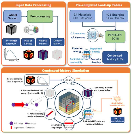
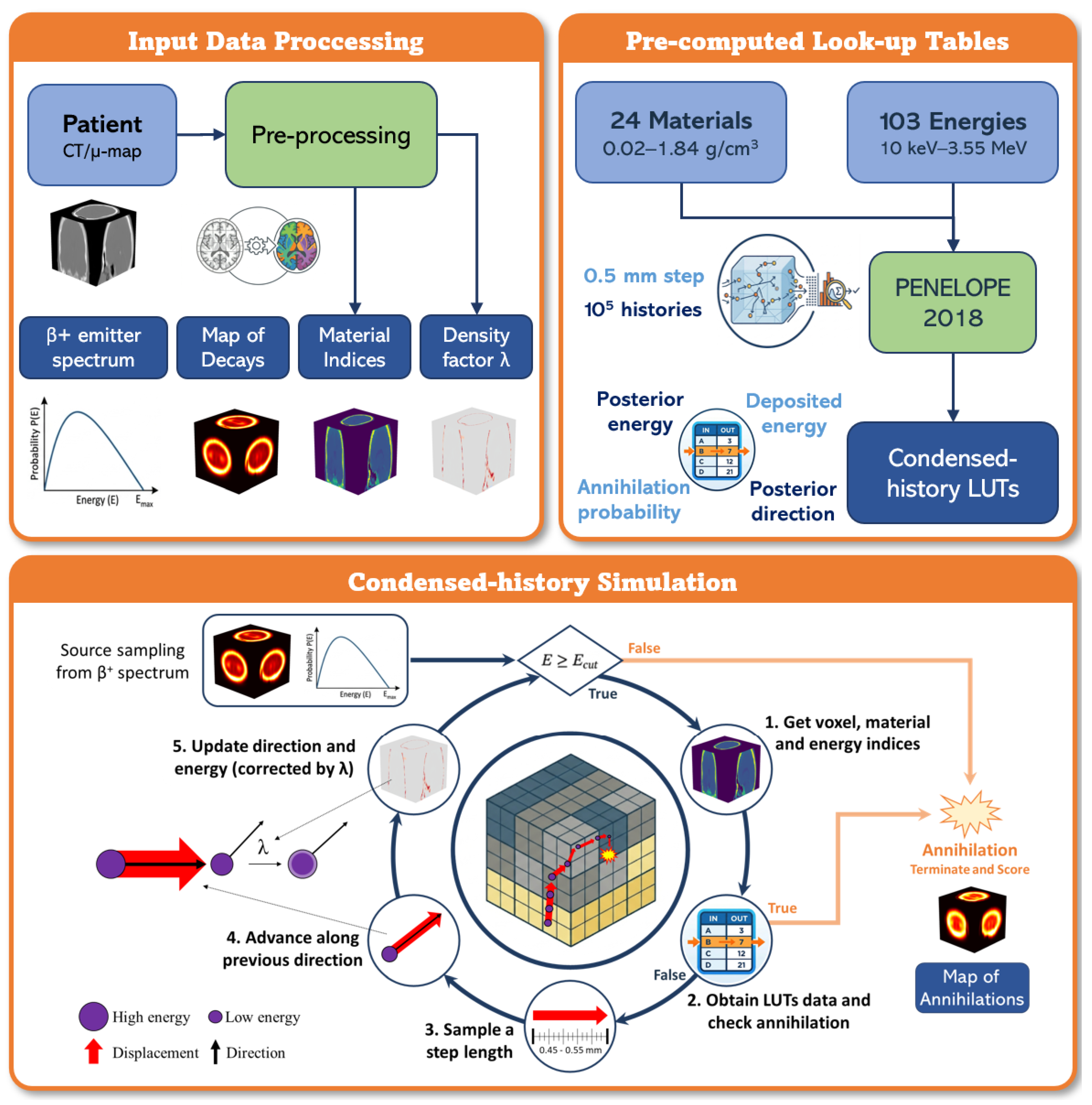
Pre-computed interaction look-up tables (LUTs) were generated offline and cover the 24 materials from Schneider and 103 logarithmically spaced energy points between 10 keV and 3.55 MeV. The tables were generated by running detailed (event-by-event) PENELOPE 2018 simulations [28] for each material and energy bin. For each combination of material m and energy index k, we tracked ${10}^5$ positron histories through a fixed step length of 0.5 mm.

The choice of 0.5 mm comes from the average standard deviation of the 99.9th percentile PR estimates across a variety of MC codes for the isotopes used in this study (¹⁸F, ⁶⁸Ga, ⁸²Rb and ¹²⁴I), which allows the use of PenEasy 2024 as the only validator [3]. We increased this average (originally 0.4 mm) by 0.1 mm to balance conservativeness with spatial resolution. To mitigate deterministic grid-alignment artefacts due to the constant step length used for LUTs, we take a similar approach to the random-hinge method in PENELOPE [28] and Berger’s condensed-history formulation [44]. At runtime, the transport step was sampled uniformly from 0.45–0.55 mm, i.e., a uniform distribution centred on the 0.5 mm step used for LUT generation. The 10% variation comes as a conservative estimate from the per cent path length straggling in [44].

From these simulations, the probability of annihilation was estimated, together with the mean energy deposited per step, and the information about outgoing energy and scattering angle, providing a sufficiently large set of possible outcomes for the condensed-history simulation. The tables encode the following quantities:

• Annihilation probability per step. $103\times 24$ entries (∼83 kB).
• Posterior energy distribution. ${10}^5\times 103\times 24$ entries (∼943 MB), where ${10}^5$ is the number of discrete samples of the outgoing energy in each combination (m, k).
• Posterior angular distribution. ${10}^5\times 103\times 24$ entries (∼943 MB), storing the corresponding scattering-angle distributions.
• Mean energy deposition per step. $3548\times 24$ values (∼2.8 MB), obtained over the 10 keV–3.55 MeV range using a 1 keV linear energy grid.

2.3. Inputs and Output

The simulator requires the following input files, all placed in the working directory:

• MATERIAL.raw (int32)—voxelised map with identifiers of materials (see Table A1);
• DENSCORR.raw (float32)—voxelised density-correction factors $\lambda$ (see Section 2.1);
• DECAY.raw (float32)—voxelised map of the number of decays per voxel;
• spectrum.txt—two-column ASCII file (energy in eV, probability) representing the ${\beta }^{+}$ emission spectrum.

The emission energy for each positron is sampled from the spectrum file via inverse-transform sampling. Spectrum files for ¹⁸F ($Q=633.5$ keV), ⁶⁸Ga ($Q=1899$ keV), ⁸²Rb ($Q=3150$ keV), and ¹²⁴I ($Q=2135$ keV) have been precomputed using the PENNUC nuclear decay code [28]. However, any user-provided spectrum can be used, enabling the simulation of additional radionuclides and specific decay branches.

Simulation parameters are specified via a plain-text configuration file (config.in) that contains the base random number generator seeds, the number of CUDA threads per block and histories-per-thread multiplier, the CPU batch size, and the transport energy cutoff $E_{\mathrm{cut}}$ (default 100 eV). The compiled executable is invoked as ./hybrid_positron_UCM.x <device> <Nx> <Ny> <Nz> <dx> <dy> <dz> where device = 1 selects GPU execution and device = 0 selects CPU execution. The command-line arguments Nx, Ny, and Nz specify the number of image voxels along the three axes, while dx, dy, and dz specify the voxel spacings in cm.

The output is a 3D annihilation map (ANNIHILATION.{gpu,cpu}.raw, float32), representing the posterior distribution of positron annihilation events. This map is directly usable as input for PET image reconstruction and resolution modelling.

2.4. Condensed-History Radiation Transport Algorithm

Each positron is transported using a condensed-history approach [28,44], in which many elastic and inelastic collisions over a fixed step are not tracked individually, but instead are represented collectively using the pre-computed LUTs of interaction probabilities and energy losses (Section 2.2). The simulator uses the RANECU combined linear congruential generator of L’Ecuyer [45], with a period of $\approx$ 2.3 ×${10}^{18}$. Each simulation history is assigned a unique, deterministic seed pair derived from the base seeds and the global history index, ensuring full reproducibility across batches and GPU/CPU execution.

Each positron history is simulated as follows:

1.

Source sampling. A source voxel is identified via binary search on the cumulative activity distribution, where each voxel is assigned an index range proportional to its activity weight, allowing histories to be sampled across voxels without requiring sequential completion. The initial position is sampled uniformly inside the source voxel, the direction is sampled isotropically ($cos\theta \in [-1,1)$, $\varphi \in [0,2\pi )$), and the initial kinetic energy is sampled from the input spectrum CDF via inverse transform.

2.

Transport loop condition. Transport continues while the kinetic energy satisfies $E\ge E_{\mathrm{cut}}$ (in keV). The history also stops immediately if the particle leaves the voxelised domain or the positron annihilates.

3.

Step length sampling. At each loop iteration, a random step length is sampled as

$$s=0.045+0.01{\xi }_1,{\xi }_1\sim \mathcal{U}(0,1),$$

(1)

where s is expressed in cm (i.e., 0.45–0.55 mm). The fixed step-size range (0.1 mm) was chosen to balance computational efficiency with spatial accuracy: it is small enough to capture sub-voxel positron transport details while remaining large enough relative to mean free paths in soft tissue to justify the condensed-history approximation at clinical scales. The fixed step size also simplifies the GPU kernel logic and avoids thread divergence, which is critical for GPU throughput.

4.

Current voxel/material and energy indexing. From the current position, voxel indices $(i,j,l)$ and material m are obtained. Energy indices are then computed:

• logarithmic index k (103 bins, $\Delta {log}_{10}E=0.025$) for annihilation probability, energy loss, and scattering angle tables;
• linear index $k^{\prime }$ (1-keV bins, up to 3548 keV) for mean deposited energy table.

5.

Interaction threshold interpolation and event decision. A threshold value is linearly interpolated from the annihilation probability table:

$$P(E,m)=P_{k,m}+(E-E_k){\displaystyle \frac{P_{k+1,m}-P_{k,m}}{E_{k+1}-E_k}},$$

(2)

where $P_{k,m}$ is the tabulated annihilation probability for an energy $E_k$ and material m, and E is the current particle energy. After sampling a random variable ${\xi }_2\sim \mathcal{U}(0,1)$,

• if ${\xi }_2\le P(E,m)$, the positron is terminated and the annihilation counter of voxel $(i,j,l)$ is incremented;
• otherwise, the positron survives and keeps being transported.

6.

Position advance. The particle is moved along its current direction:

$$\mathbf{r}\to \mathbf{r}+s\widehat{\mathbf{u}}.$$

(3)

If the new position is outside the grid, the history terminates.

7.

Post-step energy and direction update from tables. A single random number ${\xi }_3\sim \mathcal{U}(0,1)$ is used to sample from the posterior tables. For the current material and logarithmic energy bin, that row provides:

• a tabulated outgoing energy $E_{\mathrm{tab}}$;
• the polar cosine as $\mu =1-cos\theta$.

Another random number ${\xi }_4\sim \mathcal{U}(0,1)$ is also used for azimuth, $\varphi =2\pi {\xi }_4$.

The tabulated outgoing energy is first shifted from the bin-reference energy to the particle’s actual energy:

$$E_{{\mathrm{tab}}^{\prime }}=E_{\mathrm{tab}}-E_{\mathrm{ref}}+E.$$

(4)

It is then corrected with the stopping-power difference between the reference energy in that logarithmic bin and the current particle energy, scaled by the density-correction factor $\lambda$:

$$E_{\mathrm{out}}=E_{{\mathrm{tab}}^{\prime }}+\lambda \left(\Delta E_{\mathrm{dep}}\left(E_{\mathrm{ref}}\right)-\Delta E_{\mathrm{dep}}\left(E\right)\right).$$

(5)

Finally, the outgoing energy is clipped to the physical range $0\le E_{\mathrm{out}}\le E$, and the direction is rotated using $\mu$ and $\varphi$.

2.5. GPU Implementation and Optimisations

The GPU kernel follows a one-thread-per-history parallelisation strategy: each CUDA thread simulates one complete positron history, from emission to annihilation or energy cut-off, independently of all other threads. The annihilation map is accumulated via atomic additions to handle concurrent writes to the same voxel from multiple threads without race conditions. Density and material maps are stored in global memory.

Because the total number of histories can exceed the GPU thread capacity, the simulation proceeds in batches. The maximum number of histories per batch is bounded by

$$N_{\mathrm{batch}}=N_{\mathrm{thread}}\times M_{\max }\times i_{\mathrm{mult}},$$

(6)

where $N_{\mathrm{thread}}$ is the number of CUDA threads per block, $M_{\max }$ is the maximum number of blocks, and $i_{\mathrm{mult}}$ is the number of histories assigned to each thread, run one after another. Source voxels are mapped to global history indices via a prefix-sum array over the cumulative activity distribution, and each thread locates its source voxel at kernel launch by binary search on this array. Batch results accumulate on the host after each kernel call, and the final annihilation map is written to disk on completion.

Several implementation choices were adopted to improve throughput and numerical robustness:

• Shared memory table cache. The annihilation-probability table ($9.7$ kB per thread block) is staged in GPU shared memory to reduce global-memory latency.
• Constant memory. Geometry constants ($N_x$, $N_y$, $N_z$, $\Delta x$, $\Delta y$, $\Delta z$) are stored in CUDA constant memory.
• Sparse density pages. When density corrections $\lambda$ are mostly unity across specific regions (e.g., air outside the patient), the map can be stored in compact $4\times 4\times 4$ pages of active voxels to reduce memory traffic.
• Spectrum CDF search. Inverse-transform sampling of the emission spectrum uses a binary search on the cumulative distribution, resulting in $\mathcal{O}(logN)$ complexity.
• Deterministic batching. Seeds and history indices are derived deterministically per batch and per thread/history, enabling reproducible CPU/GPU comparisons under fixed inputs.
• Fast math. The code is compiled with the fastmath flag to exploit floating-point hardware units at full throughput.

2.6. Validation

The HMC simulator was validated in both CPU and GPU modes against PenEasy 2024 [29], which is based on PENELOPE 2023 [28], in five complementary dimensions: point-source spread behaviour and convergence, heterogeneous interface response, a ⁸²Rb myocardium annihilation-distribution simulation from a clinical [¹⁸F]FDG acquisition [41], and runtime performance. PenEasy 2024 was chosen as the validation reference because, in our recent work [3], PR distributions computed with PenEasy/PeneloPET were systematically benchmarked against GEANT4 (via GATE) and PHITS for the same ${\beta }^{+}$ emitters considered here in water, yielding agreements within 5–10% across codes.

The validation objective was not to establish statistical superiority but to test whether HMC reproduces the reference trends and magnitudes observed with PenEasy under shared geometrical and radionuclide scenarios. The setup for PenEasy was designed to use the same inputs as HMC: equal voxelised geometry, same lower energy threshold for positron transport (100 eV), and equivalent emission energy and spatial distribution using a phase space file (source.psf) that was generated with Python 3.13 using np.random.choice and the same decay image. Additionally, the tracking of electrons and photons in PenEasy was minimised by assigning an absorption energy threshold of 10 MeV. Transport parameters of PenEasy were kept at default ($C_1=C_2=0.1$, $W_{cc}=100$ keV and $W_{cr}=10$ keV).

Point-source analysis used axially projected displacement-from-centre voxel profiles, stratified by radionuclide and material, together with normalised annihilation-density curves. These simulations used a grid of $121\times 121\times 121$ voxels and a voxel side of 1.5 mm. The odd number of voxels per dimension places the point source in the centre of the grid’s central voxel. The convergence analysis evaluated FWHM and FWTM over increasing history counts and computed width residuals relative to PenEasy, reported in millimetres for all metrics. FWHM and FWTM were computed directly from the discrete profiles without fitting an analytical function. The peak amplitude was taken as the maximum sample value and a threshold was set at a fixed fraction of the peak (0.5 for FWHM, 0.1 for FWTM). The threshold-crossing positions on either side of the peak were located by linear interpolation between adjacent samples, and the full width taken as the difference between them. The uncertainty of each FWHM/FWTM estimate is obtained using a Poisson bootstrap with 200 samples to assess its variability. The standard deviation $\sigma$ from all bootstrap samples is used to calculate the uncertainty.

For the sphere-interface tests, a grid of $420\times 420\times 420$ voxels with 1.5 mm side was used. Spheres were defined with a 10 mm radius and centred at the origin. In this scenario, the origin is specified as the common intersection point of the 8 central voxels. Thus, the even number of voxels per dimension ensures a symmetric material interface and the same number of decays in each material. The total number of decays was initially set to ${10}^7$, although the actual number depends on the material.

The myocardium benchmark used clinical data of [¹⁸F]FDG PET/CT images [41]—cropped to a $86\times 86\times 86$ voxel grid with $1.65\times 1.65\times 2.00$ mm³ per voxel representing the myocardial region—as the decay input for ⁸²Rb simulations. The number of decays in this image was scaled to a total of $4.52·{10}^8$. The agreement with PenEasy 2024 was quantified using global MAE, RMSE, SSIM, PSNR and linear regression, as well as voxelwise relative error and local SSIM (using a 3 × 3 × 3 moving window).

The results from PenEasy 2024 and HMC (CPU/GPU) are compared with a naive Gaussian-blur of the initial decay image, choosing the blur sigma equal to the mean PR of the respective isotope in water, averaged across a variety of MC codes [3]. To account for uptake concentration in soft-tissue we have increased the number of decays in water (soft tissue) with respect to bone and lung tissues, using an arbitrary ratio of 1 (bone/lung) to 5 (water). This increase helps to not always consider a symmetric Gaussian blur. The profiles were organised by material ordering (e.g., lung|bone, lung|water, water|bone), and the left–right asymmetry terms were computed as the total number of annihilations within each material.

2.7. Use of GenAI

The use of generative artificial intelligence (GenAI) in this work has been limited to manuscript drafting and review, coding assistance, and auxiliary image generation in Figure 1 (specifically, using Gemini 3.1 Pro to create the Pre-processing, PENELOPE 2018 and LUT icons, which are used solely for visual aesthetics). It was strictly used as a time-saving method and did not interfere in any case with the scientific judgement of the authors. All outputs were reviewed, validated and edited under human supervision.

Figure 1. Overview of the HMC pipeline, showing input preprocessing, look-up table generation, and condensed-history transport algorithm to generate a 3D annihilation map.

3. Results

3.1. Point-Source Profile Agreement

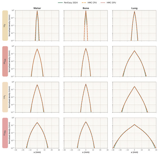
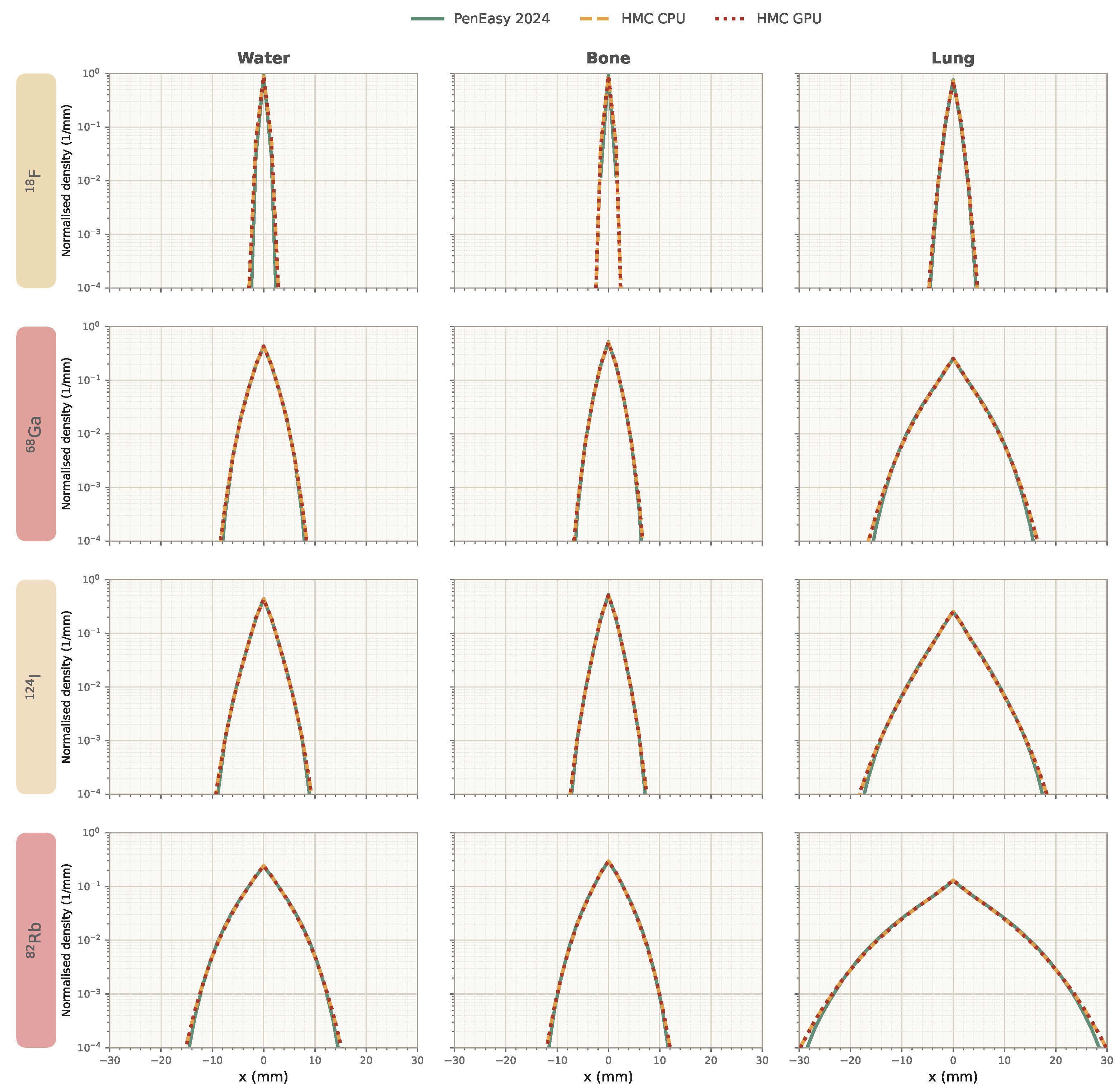
As shown in Figure 2, point-source profiles from HMC (CPU and GPU) and PenEasy 2024 presented the same overall behaviour across radionuclides and materials: a shared central-peak structure followed by smooth outward attenuation. In general, HMC begins to deviate from PenEasy once the profiles have undergone an attenuation of three orders of magnitude. The dominant profile shapes and peak locations were visually consistent across codes, supporting agreement in the primary transport pattern.

Figure 2. Point-source annihilation density profiles projected over the x-axis for ¹⁸F, ⁶⁸Ga, ⁸²Rb, and ¹²⁴I in water, lung, and bone (see Section 2.1), comparing HMC CPU, HMC GPU, and PenEasy 2024 after ${10}^7$ histories simulated. The bin size equals the voxel size (1.5 mm). HMC CPU and GPU exhibit nearly identical behaviour, and reach slightly larger distances than PenEasy 2024.

3.2. Convergence Width Residuals

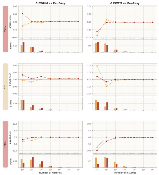
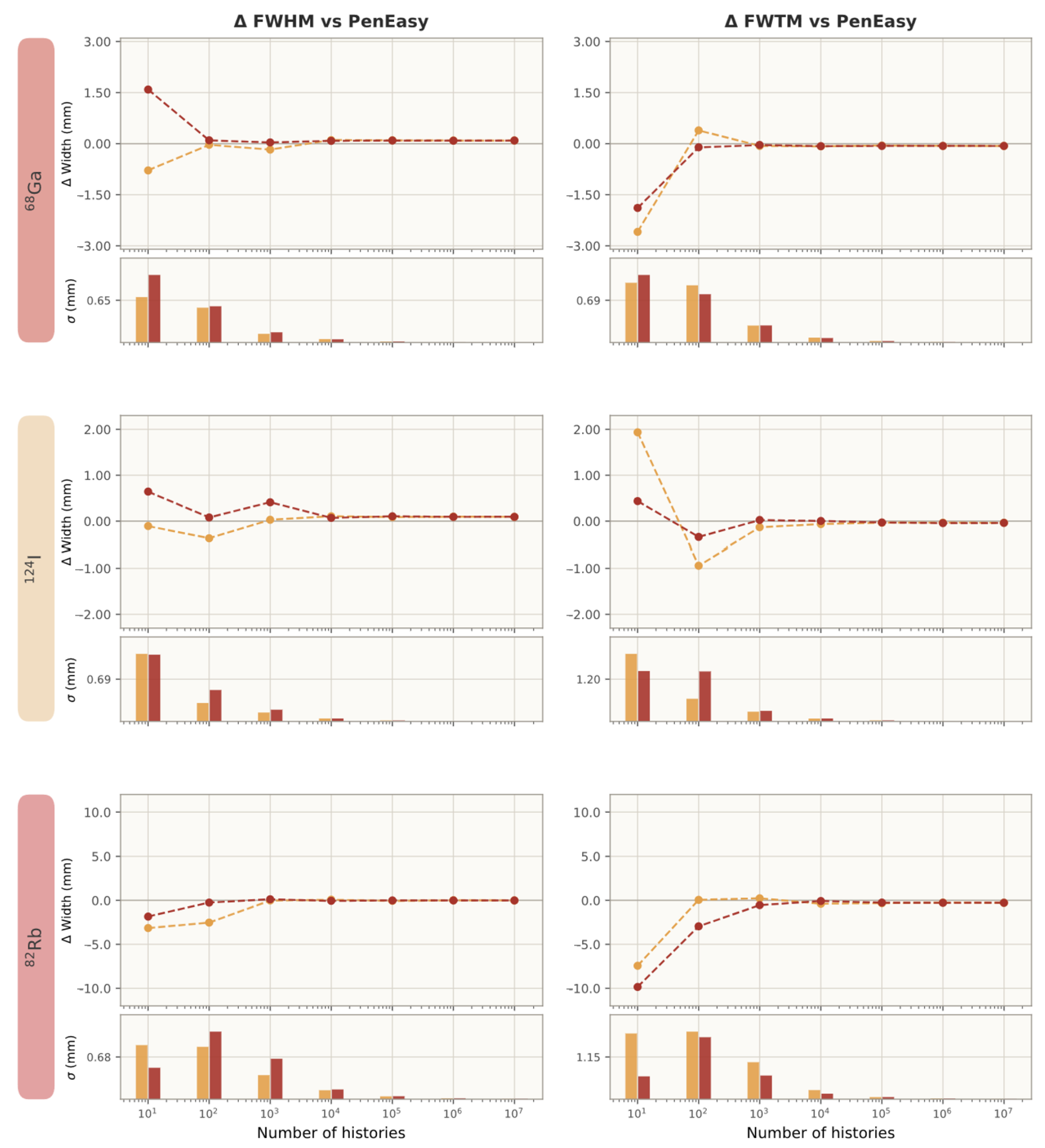
Convergence residuals against PenEasy (Figure 3, Table 1) were small in absolute magnitude at the highest history level ($n_{\mathrm{hist}}={10}^7$). For ⁶⁸Ga, FWHM residuals were $+0.090$ mm (HMC-CPU) and $+0.092$ mm (HMC-GPU), while FWTM residuals were $-0.066$ mm and $-0.067$ mm. A similar trend is followed by ¹²⁴I. For ⁸²Rb, FWHM residuals were $-0.009$ mm (CPU) and $-0.006$ mm (GPU), and FWTM residuals were $-0.271$ mm and $-0.272$ mm. Across nuclides, CPU and GPU residual endpoints were closely matched (Figure 3), indicating that the device choice had limited effect on the final convergence-width disagreement with PenEasy, which is then related to the condensed-history implementation. However, the combined pattern was consistent with stable high-history behaviour and limited absolute residual bias ($\left|\Delta \mathrm{FWHM}\right|<$ 0.1 mm and $\left|\Delta \mathrm{FWTM}\right|<$ 0.3 mm).

Figure 3. FWHM and FWTM residuals (difference with respect to PenEasy at ${10}^7$ histories) from HMC CPU (orange) and GPU (red) point-source simulations in water as a function of history count for ⁶⁸Ga, ¹²⁴I, and ⁸²Rb in water. The bin size used for FWHM/FWTM equals the voxel size (1.5 mm). Uncertainties $\sigma$ of each FWHM/FWTM estimate are estimated as the standard deviation from 200 Poisson bootsrtaps.

Table 1. Convergence of FWHM and FWTM (mm) at $n_{\mathrm{hist}}={10}^7$ for HMC CPU, HMC GPU, and PenEasy 2024 in water, bone, and lung. Notice that ${\rho }_e·$ FWHM/FWTM yields closer values across all materials for the same isotope, as expected from 1D PR proportionality with density [3].

Nuclide	Material	FWHM (mm)			FWTM (mm)
		HMC-CPU	HMC-GPU	PenEasy	HMC-CPU	HMC-GPU	PenEasy
68Ga	Water	2.75	2.75	2.66	7.47	7.47	7.54
	Bone	2.45	2.45	2.34	5.89	5.89	5.87
	Lung	4.37	4.37	4.26	13.58	13.59	13.87
124I	Water	2.70	2.70	2.61	7.33	7.32	7.36
	Bone	2.41	2.41	2.28	5.85	5.85	5.80
	Lung	4.38	4.38	4.29	13.23	13.23	13.51
82Rb	Water	4.83	4.83	4.84	13.77	13.76	14.04
	Bone	4.10	4.11	4.00	10.94	10.94	11.08
	Lung	8.08	8.10	8.27	26.83	26.84	27.50

At lower history counts, the observed deviations are dominated by statistical fluctuations rather than by algorithmic differences. The Poisson noise in the sparsely populated projected profiles introduces bin-to-bin variations that propagate into the FWHM/FWTM calculation, producing the oscillatory residual pattern visible in the early stages of Figure 3. Both HMC and PenEasy profiles are affected, and the bootstrap-based uncertainty estimates shown in the $\sigma$ subpanels of Figure 3 confirm that these early-stage deviations lie within the counting-statistics envelope. As the number of histories increases, the statistical noise is progressively reduced and the systematic residual due to the condensed-history approximation emerges as the dominant component, converging to the stable endpoint values reported in Table 1.

Table 2 shows the validity of the simulated FWHM and FWTM estimates against the experimental work by Anton-Rodriguez et al. [46], where point ¹⁸F and ⁶⁸Ga sources emitted positrons that were transported across acrylic. To compare our simulations with the experimental values, we scaled them using the electronic density ${\rho }_e=Z/A·\rho$ considering a mass density 1.20 g/cm³ and composition ${\mathrm{C}}_5{\mathrm{H}}_8{\mathrm{O}}_2$ [3,47]. We observe a general agreement below 15% except for the FWTM of ⁶⁸Ga, where the simulation overestimates its value a ∼56%.

Table 2. Comparison of simulated and experimental FWHM and FWTM values scaled by electronic density for ¹⁸F and ⁶⁸Ga and the relative differences of simulations compared to experimental. The experimental values come from [46].

Nuclide	Code	FWHM (g/cm2)			FWTM (g/cm2)
		Sim	Exp	$\Delta$ (%)	Sim	Exp	$\Delta$ (%)
18F	PenEasy	0.866	0.838	3.32	1.558	1.687	−7.60
	HMC	0.898		7.20	1.617		−4.13
68Ga	PenEasy	1.487	1.344	10.62	4.216	2.677	57.46
	HMC	1.537		14.38	4.179		56.08

3.3. Sphere Interface: Localisation of Differences

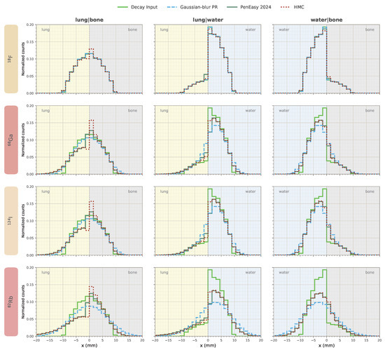
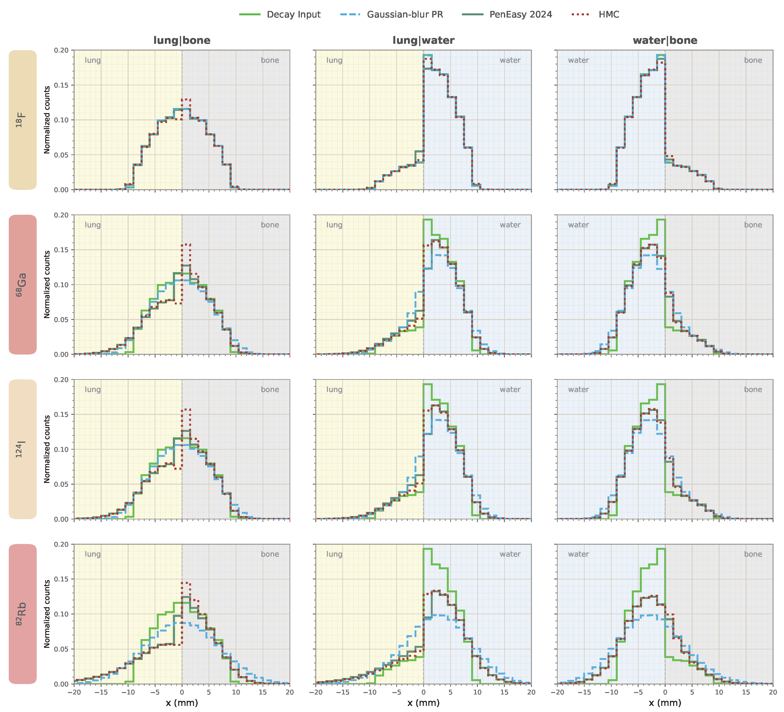
Figure 4 shows that the discrepancies with respect to PenEasy 2024 were mainly confined to the interface region. Most of the absolute difference mass concentrated in the border region ($\left|x\right|\le 5$ mm) rather than in the outer region ($\left|x\right|\ge 10$ mm) of the spheric source. The asymmetry ratios in Table 3 provide complementary information on how each method redistributes annihilation counts across the interface. In most cases, HMC remains close to PenEasy 2024, with the strongest deviations appearing for the lung|bone configurations and smaller differences for the lung|water and the water|bone interfaces. We also observe that the naive Gaussian-blur PR approach fails to replicate abrupt material-transition phenomena and generally overestimates the PR effect in the case of ⁸²Rb, with higher counts than PenEasy in regions far from the interface.

Figure 4. Annihilation density profiles, projected over the x-axis, of sphere phantoms on heterogenous tissue (lung|bone, lung|water, water|bone, ${420}^3$ voxels, 1.5 mm size) for ¹⁸F, ⁶⁸Ga, ⁸²Rb, and ¹²⁴I, comparing HMC and PenEasy against the input profile and a naive Gaussian-blur approximation of the PR effect (setting $\sigma$ as the mean PR for that isotope in water). Spheres have a 10 mm radius, initially homogeneous number of decays (total of ${10}^7$) and are centred at the intersection of the 8 central voxels. The number of decays happening in water is scaled by a factor 5 to account for uptake concentration in soft-tissue and allow asymmetric Gaussian-blur distribution. The bin size equals the voxel size.

Table 3. Sphere interface asymmetry ratios ($L/R$) of annihilations, computed as the sum of profile counts on the left half material ($·|$) divided by the sum on the right half material ($|·$).

Nuclide	Interface	Decay Input	Gaussian-Blur PR	PenEasy 2024	HMC
18F	lung|bone	1.00	1.00	1.01	0.95
	lung|water	0.20	0.20	0.23	0.21
	water|bone	5.00	4.97	4.81	4.68
68Ga	lung|bone	1.00	1.00	0.92	0.79
	lung|water	0.20	0.35	0.31	0.26
	water|bone	5.00	2.88	3.39	3.34
124I	lung|bone	1.00	1.00	0.93	0.79
	lung|water	0.20	0.35	0.31	0.26
	water|bone	5.00	2.87	3.40	3.34
82Rb	lung|bone	1.00	1.00	0.86	0.73
	lung|water	0.20	0.50	0.41	0.34
	water|bone	5.00	2.01	2.50	2.48

Several approaches have been tested to reduce this discrepancy in the interface regions between HMC and PenEasy (boundary-aware energy loss in simulations, density blurring pre-process to soften material heaps, higher-order corrections in DENSCORR.raw), but none improved the overall results. However, since decay density is generally higher in soft tissue than in lung, the resulting effects partially offset one another (with two tissues $t_1$ and $t_2$ with densities ${\rho }_1<{\rho }_2$ and identical number of decays $n_1=n_2$, the net flux of annihilation probability near the interphase goes from $t_1$ to $t_2$. If we swap to the ${\rho }_1={\rho }_2$ and $n_1<n_2$ case, the flux reverses from $t_2$ to $t_1$. Therefore, we can expect a partial offset of both effects when ${\rho }_1<{\rho }_2$ and $n_1<n_2$). This offset is particularly relevant in the water|bone interface when considering a ratio 1 (bone) to 5 (water) in activity concentration (see Figure 4).

3.4. Myocardium Validation Benchmark

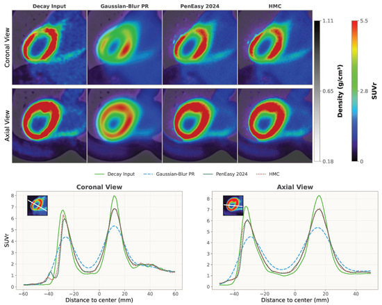
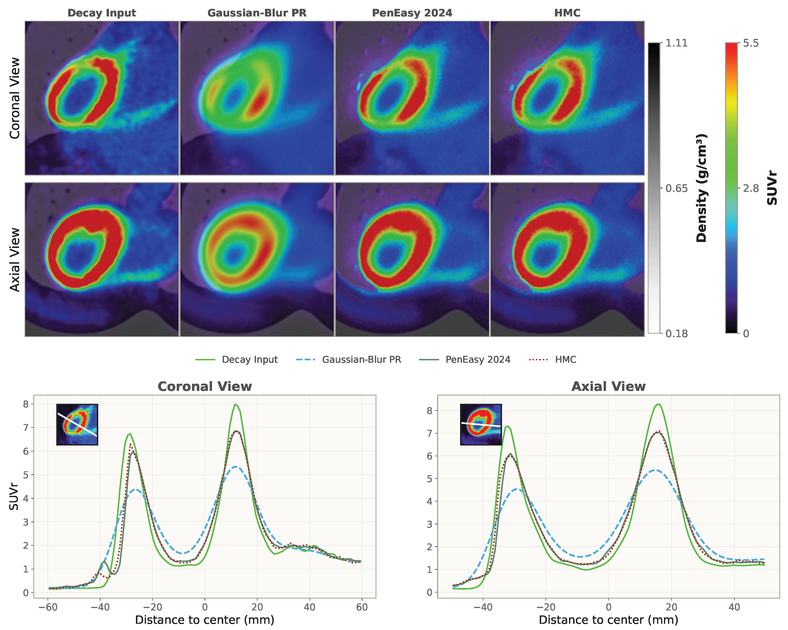
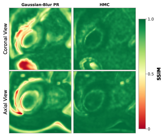
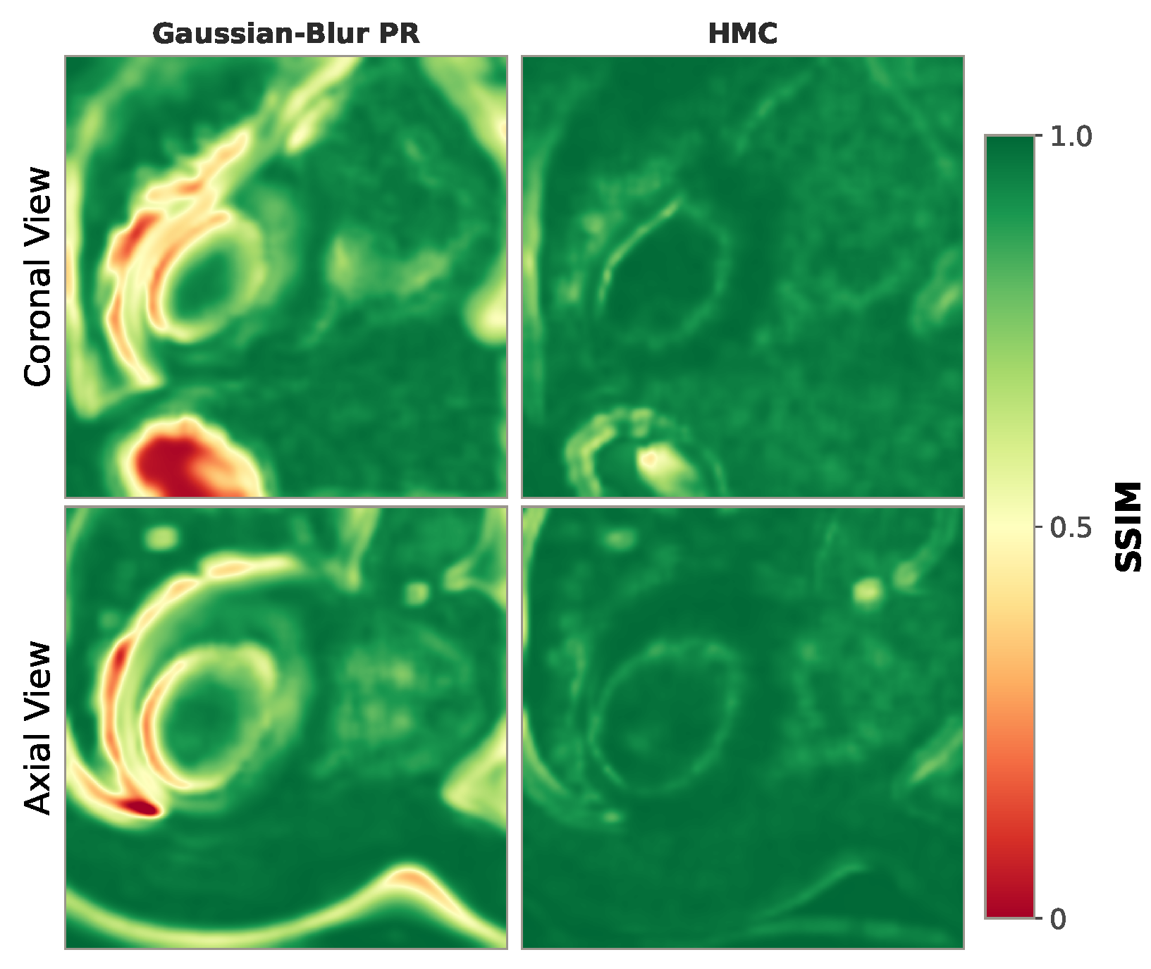
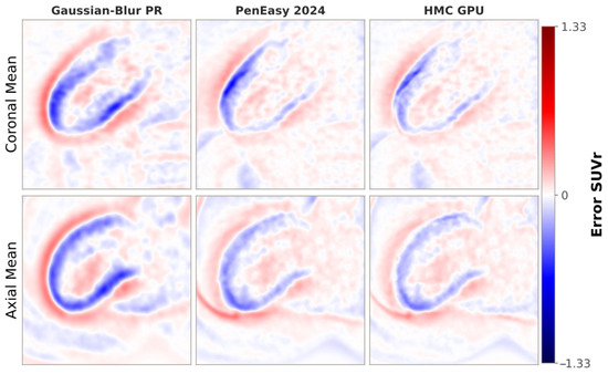
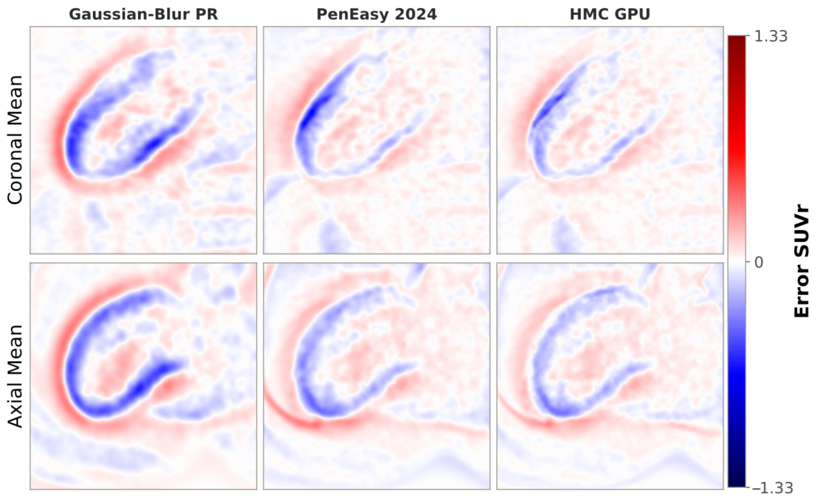
Across the myocardium benchmark, global error metrics (Table 4) were generally good for both naive Gaussian-blur and HMC methods relative to PenEasy 2024. While MAE and RMSE are approximately 3-fold lower in HMC than Gaussian-blur, the PSNR of the resulting image is 30% better with a global SSIM also notably improved from $0.956$ to $0.995$. The biggest improvement is seen in voxelwise relative error metrics, which decreased one order of magnitude using HMC. Across all the metrics, both backends for HMC show almost equal results. Voxelwise linear regression likewise showed very strong agreement between PenEasy and the HMC backends ($R^2=0.995$), and a slightly weaker match for Gaussian-blur PR ($R^2=0.964$). The visual maps and profiles in Figure 5, Figure 6 and Figure 7 indicate a high global agreement with localised residual patterns rather than broad discrepancies using HMC. Minor differences appear in the lung region in the coronal view (Figure 5, Figure 6 and Figure 7), likely due to the larger PR in low-density tissue magnified by a more asymmetric PR distribution near tissue interfaces than expected.

Table 4. Myocardium benchmark summary for HMC and Gaussian-blur PR relative to PenEasy 2024, combining global and relative error metrics.

	Global Error Metrics				Relative Error Metrics
vs. PenEasy	MAE	RMSE	SSIM	PSNR (dB)	Mean	Std	Median	${\mathit{p}}_{\mathbf{95}}$ abs
Gauss-blur	0.163	0.298	0.956	27.787	0.119	1.855	$-0.016$	1.031
HMC CPU	0.061	0.110	0.995	36.436	0.012	0.175	$-0.001$	0.333
HMC GPU	0.061	0.110	0.995	36.438	0.012	0.175	$-0.001$	0.333

Figure 5. (Upper) Annihilation and real density maps in the myocardium benchmark (⁸²Rb, ${86}^3$ voxels, 1.65 mm side). Our simulator (HMC) shows strong visual agreement with PenEasy 2024, which serves as expected outcome. Slight discrepancies are visible in lung regions of the coronal view. (Lower) Line profiles through the myocardium annihilation map (${86}^3$ voxels, 1.65 mm side) comparing our method (HMC, dotted red), against a naive Gaussian-blur PR estimate (dashed cyan) and a reference MC simulation with PenEasy 2024 (solid dark green). The initial decay profile (solid lime) is also shown for comparison. The bin size equals the voxel size (1.65 mm). Our approach, that takes 1 s in GPU and 14 min in CPU, attains performance that is nearly identical to that of the full MC simulation (8 h 45 min). Discrepancies are mostly visible in lung regions.

Figure 6. Structural similarity index metric (SSIM) maps comparing naive Gaussian-blur PR and HMC (CPU/GPU) against PenEasy 2024 for the myocardium benchmark. HMC shows high SSIM values across the volume, with localised reductions in the lung region. Voxelwise SSIM was computed using a 3 × 3 × 3 moving window.

Figure 7. Difference maps against the original decay distribution for the myocardium benchmark (${86}^3$ voxels, 1.65 mm side). A naive Gaussian-blur PR estimate differs significantly from a MC simulation using PenEasy 2024. Our method (HMC) achieves similar results using condensed-history MC.

3.5. Runtime Behaviour

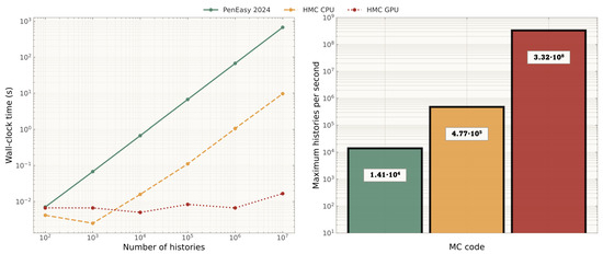
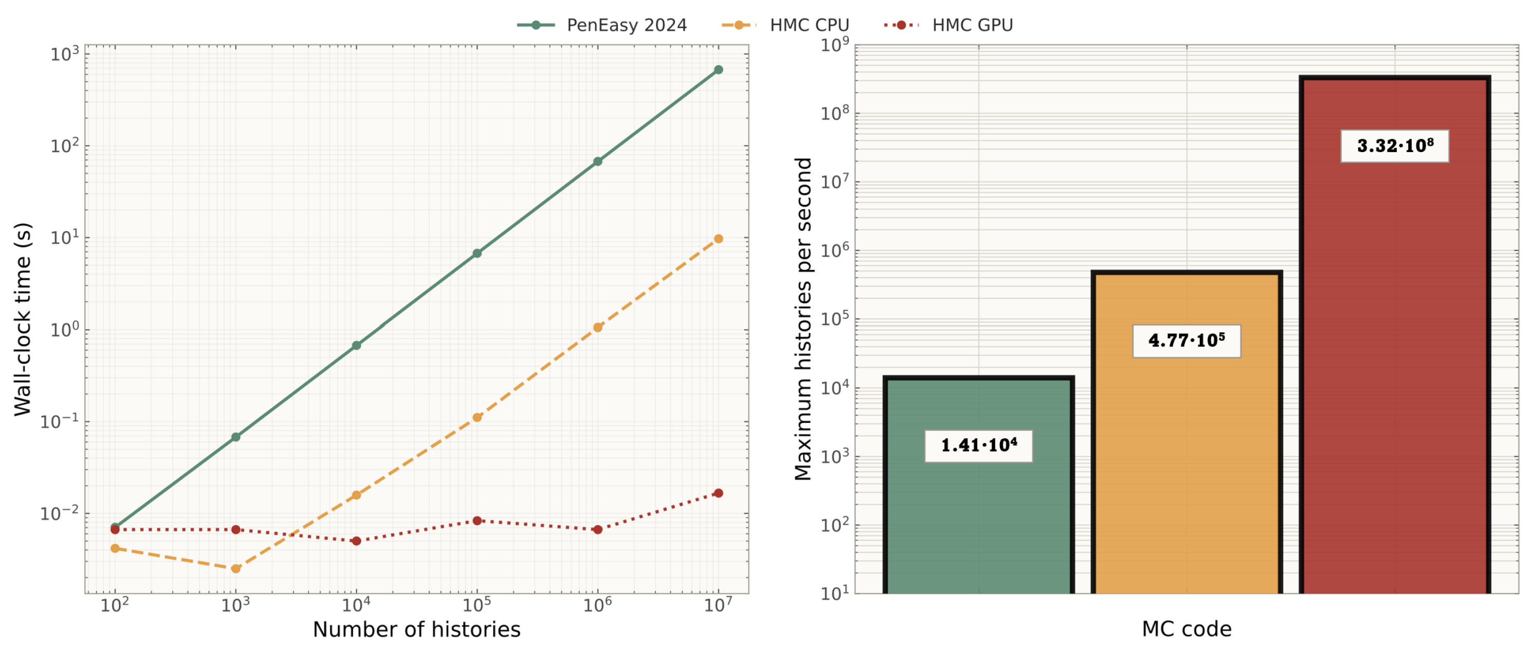
The runtime behaviour (Figure 8) showed a clear separation of the backend in the tested histories (the increase of runtime with the number of histories is linear, as expected from the $\mathcal{O}\left(N\right)$ algorithmic complexity of MC radiation transport.) In the point-source benchmarks, runtime remained ordered with PenEasy 2024 highest, HMC CPU intermediate, and HMC GPU lowest over the sampled range. Table 5 reports the throughput values from the myocardium benchmark with ⁸²Rb. The terminal (maximum) simulation speeds were $3.32·{10}^8$ histories/s for HMC GPU (NVIDIA RTX 5080), $4.77·{10}^5$ histories/s for HMC CPU (Intel i9-14900KF), and $1.41·{10}^4$ histories/s for PenEasy 2024 (idem). HMC CPU algorithmic improvement over PenEasy 2024 is $34\times$, attributable to the condensed-history approximation. Additionaly, HMC GPU gain from GPU parallelism is $697\times$ relative to HMC CPU, resulting in a combined speedup of $23,600\times$ relative to single-thread PenEasy 2024.

Figure 8. (Left) Runtime as a function of history count and (right) maximum simulation speed (histories per second) for PenEasy 2024 (green), HMC CPU (orange), and HMC GPU (red).

Table 5. Terminal simulation throughput and relative speedup for the myocardium benchmark.

	HMC GPU	HMC CPU	PenEasy 2024
Hardware	NVIDIA RTX 5080	Intel i9-14900KF
CUDA toolkit/Compiler	nvfortran 26.1		ifx 2025.3.0
Wall-clock time (s)	1.06	876	31,439
Speed (${10}^3$ histories/s)	$3.32·{10}^5$	477	$14.1$
Speedup vs. PenEasy	$2.36·{10}^4$	$33.9$	1

4. Discussion

4.1. Summary of Findings

The main objective of this work was to develop and validate a GPU-accelerated condensed-history Monte Carlo simulator for explicit positron transport through heterogeneous voxelised media. The validation results presented above demonstrate that the HMC simulator reproduces PenEasy reference behaviour across multiple test scenarios with close quantitative agreement. The strongest concordance was observed in the realistic myocardium phantom, where both HMC backends achieved voxelwise $R^2=0.995$, $\mathrm{SSIM}=0.995$ and PSNR values near 36.4 dB. These results indicate that the condensed-history transport model faithfully captures the aggregate positron transport physics in heterogeneous media, including the complex interplay between energy loss, scattering, and annihilation that determines the spatial distribution of annihilation events.

The choice of PenEasy 2024 as the validation reference is grounded in our prior cross-code benchmark of PR distributions [3], where PenEasy/PeneloPET were systematically compared against GEANT4 (via GATE) and PHITS for the same four ${\beta }^{+}$ emitters considered in this work, in homogeneous water and a water|bone interface. That study established mutual agreement of multiple MC codes within 0.5 mm across these radionuclides in homogeneous water, which fits with the chosen LUT step size. Specifically, the maximum standard deviation between MC codes was found for the 99.9th PR percentile estimate, which is 0.11 mm for ¹⁸F, 0.39 mm for ⁶⁸Ga, 0.44 mm for ¹²⁴I, and 0.68 mm for ⁸²Rb. Therefore, PenEasy has already been anchored to independent codes and does not serve as a single arbitrary reference. However, we note that this prior cross-code agreement quantification was established for homogeneous media and that sharp material interfaces show only qualitative discrepancies that need further investigation.

Point-source profiles confirmed that HMC preserves the characteristic shape of annihilation distributions across all tested radionuclides and materials. The shape of these profiles is determined by the positron energy spectrum, the stopping power of the medium, and the angular distribution of scattering events; therefore, the observed agreement provides evidence that HMC correctly reproduces all three contributions. Convergence analysis showed that FWHM residuals relative to PenEasy remained below 0.1 mm for ⁶⁸Ga and ¹²⁴I at ${10}^7$ histories, with slightly larger FWTM residuals for ⁸²Rb ($-0.27$ mm). While the CPU and GPU backends showed consistent residual patterns, the larger FWTM residuals for ⁸²Rb may indicate limitations in the high-energy tail treatment, where the condensed-history approximation and LUT discretisation (0.5 mm steps for generation) have the greatest impact.

The sphere-interface experiments revealed that code-to-code disagreements concentrate near material boundaries, as expected for condensed-history approximations. Systematic underestimation of asymmetry ratios by 13–15% across all configurations (see Table 3) suggests that HMC produces more asymmetric annihilation distributions at interfaces than PenEasy, which is visible in Figure 4. We have attempted to implement a strict boundary-crossing algorithm within the transport kernel (Section 3.3), but the overall interface response did not improve. This persistent bias is then attributable to the step chosen for the generation of LUTs (0.5 mm), which may be too coarse to capture the abrupt changes in annihilation probability near interfaces. However, as mentioned in Section 2.2, decreasing this step would make LUTs more dependent on the MC code chosen to generate them.

4.2. Comparison with Prior Work

A key advantage of the HMC simulator over existing CPU-based positron transport codes is its GPU-accelerated execution. As documented in a recent comprehensive review of GPU-based MC platforms for medical imaging [31], GPU acceleration has enabled speedups of several orders of magnitude in MC simulation across modalities. The runtime results presented here showed consistent speed ordering, with HMC GPU being the fastest backend, followed by HMC CPU, and PenEasy being the slowest. This acceleration is achieved through the one-thread-per-history parallelisation strategy, shared-memory caching of the annihilation probability table, and the use of atomic operations for annihilation scoring. The CUDA Fortran implementation allows the same source code to be compiled for both GPU and CPU targets, facilitating cross-validation and ensuring that the physics model is identical across backends. This dual-target capability is particularly valuable during development and debugging, as it allows any discrepancy to be attributed to numerical rather than physical differences.

Several other GPU-accelerated MC codes have been developed for PET imaging applications. MC-GPU-PET [37] provides real-time simulation of the full PET acquisition chain, including photon transport and detector modelling, achieving simulation speeds of more than 100 million detected coincidences per second. However, MC-GPU-PET does not perform explicit positron transport; instead, PR effects are incorporated analytically. Similarly, gPET [38] offers a complete GPU-based PET simulator with validated photon physics but relies on pre-sampled PR distributions rather than step-by-step transport. UMC-PET [39], developed within our research group, includes PR effects via pre-computed distributions and focuses on the full PET simulation pipeline including detector response and list-mode data generation. In contrast, HMC is specifically designed for detailed condensed-history positron transport through heterogeneous voxelised media, providing spatially resolved 3D annihilation kernels that can serve as input to any PET reconstruction framework. This specialisation enables a more detailed characterisation of PR effects at tissue interfaces, which cannot be captured by pre-sampled distribution approaches that assume material homogeneity.

The design choice of using pre-computed interaction tables deserves further discussion. The tables require significant offline storage (∼1.9 GB for energy and angular distributions), which must be loaded into GPU global memory at the start of each simulation. Although it takes less than 0.1 s using an RTX 5080, older GPUs could require significantly more time to complete the same task. However, this approach enables very fast in-simulation lookups based on inverse-transform sampling and avoids the computational overhead of evaluating cross-section models at each transport step. This trade-off is well suited for scenarios where many simulations must be performed with the same material library, such as systematic studies of PR across radionuclides or patient-specific resolution modelling in clinical PET imaging. Furthermore, the tables can be extended to additional materials without modifying the transport kernel, since the same condensed-history algorithm applies regardless of the number of tabulated materials.

Additionally, the high computational efficiency of the HMC simulator provides a platform for use in clinical image reconstruction workflows similar to [7,48,49]. Specifically, it could help create spatially varying PSF kernel libraries. These kernels, computed for several radionuclides in heterogeneous tissue regions, would enable better positron range correction in the reconstruction process that would lead to improved overall quantitative accuracy and spatial resolution of clinical PET images.

4.3. GPU Memory Requirements and Portability

The main GPU memory requirement is the pre-computed LUT, whose two largest components are the posterior energy and angular distributions (Section 2.2). Each is stored as a ${10}^5\times 103\times 24$ single-precision array. Together, they occupy 1.84 GiB (1.98 GB) and are loaded into GPU memory at initialization. This footprint is fixed and independent of image size. The remaining memory usage is dominated by voxel-wise arrays, stored as 32-bit maps, i.e., 4 bytes per voxel, and therefore scales linearly with image size. The three main maps used during transport, MATERIAL.raw, DENSCORR.raw, and ANNIHILATION.raw, require approximately 31 MB for a $128\times 128\times 159$ volume and 0.37 GB for a $440\times 440\times 159$ volume. Including the source map and auxiliary arrays, this increases to approximately 60 MB and below 0.8 GB, respectively.

Including CUDA runtime overhead, the practical minimum GPU memory requirement is approximately 2.5–3 GB, depending on the volume size. We therefore recommend a CUDA-capable GPU with at least 4 GB of VRAM. Thus, from a memory standpoint, the method is compatible with common mid-range consumer GPUs. Portability is mainly limited by CUDA support, as non-CUDA accelerators would require a dedicated port.

4.4. Future Work

Future work will proceed along several lines. First, comparison with experimental PR measurements (e.g., Derenzo-style polyurethane foam profiles, or published annihilation distributions for ⁶⁸Ga and ¹²⁴I) will offer an independent assessment beyond code-to-code benchmarking. Second, the systematic interface bias identified in Section 3.3 warrants a joint sensitivity study of LUT step size and density-correction order, together with a cross-code validation of the sphere-interface benchmark against GATE. Third, extending the material library to titanium and ceramics will broaden applicability to patients with implants. Finally, integration of the 3D annihilation kernels into iterative PET reconstruction will enable end-to-end quantification of the resolution-recovery and SUV-accuracy gains that motivate the present work, including a comparison against existing analytical PR kernels [3] to determine the regimes in which full MC-based correction is clinically warranted.

5. Conclusions

In this work, a GPU-accelerated Monte Carlo PR simulator was developed and validated. The code, implemented in CUDA Fortran, performs explicit condensed-history transport of positrons through 3D heterogeneous voxelised media derived from CT images or $\mu$-maps. Pre-computed interaction tables covering 24 tissue materials from air to cortical bone are used for efficient sampling of annihilation probabilities, energy losses, and scattering angles. Although demonstrated here for four clinically relevant ${\beta }^{+}$ emitters (¹⁸F, ⁶⁸Ga, ⁸²Rb, ¹²⁴I), the simulator accepts any user-provided emission spectrum.

Comprehensive validation against PenEasy 2024 demonstrated close agreement across all tested scenarios. Point-source profiles showed consistent axial profile behaviour across radionuclides and materials. Convergence analysis yielded FWHM residuals below 0.1 mm for ⁶⁸Ga and ¹²⁴I at ${10}^7$ histories. Sphere-interface experiments confirmed that code-to-code differences are located near material boundaries. In a myocardium benchmark, voxelwise $R^2$ and SSIM reached 0.995 with PSNR near 36.4 dB for both GPU and CPU backends. The GPU execution path achieved speedup factors of 23,600× relative to single-thread PenEasy 2024 while maintaining equivalent physical accuracy.

The resulting 3D annihilation maps are directly usable for PET image reconstruction and resolution modelling. Future work will focus on adaptive stepping at material interfaces, comparison against experimental PR measurements, and integration into iterative PET reconstruction frameworks for end-to-end resolution recovery evaluation.

References

- Levin, C.S.; Hoffman, E.J. Calculation of positron range and its effect on the fundamental limit of positron emission tomography system spatial resolution. Phys. Med. Biol. 1999, 44, 781–799. [Google Scholar] [CrossRef] [Scilit] [PubMed]
- Cal-González, J.; Herraiz, J.L.; España, S.; Corzo, P.M.G.; Vaquero, J.J.; Desco, M.; Udías, J.M. Positron range estimations with PeneloPET. Phys. Med. Biol. 2013, 58, 5127–5152. [Google Scholar] [CrossRef] [Scilit] [PubMed]
- Paneque-Yunta, R.J.; Encina-Baranda, N.; Carter, L.M.; Galve, P.; Ibáñez, P.; Abushab, K.M.; Udías, J.M.; Herraiz, J.L. Analytical positron range model for PET with cross-code Monte Carlo benchmarking. Phys. Med. Biol. 2025, 70, 165013. [Google Scholar] [CrossRef] [Scilit]
- Conti, M.; Eriksson, L. Physics of pure and non-pure positron emitters for PET: A review and a discussion. EJNMMI Phys. 2016, 3, 8. [Google Scholar] [CrossRef] [Scilit] [PubMed]
- Derenzo, S.E. Positron range and the fundamental limit of positron emission tomography. IEEE Trans. Nucl. Sci. 1986, 33, 565–569. [Google Scholar] [CrossRef] [Scilit]
- Jødal, L.; Le Loirec, C.; Champion, C. Positron range in PET imaging: Non-conventional isotopes. Phys. Med. Biol. 2014, 59, 7419–7434. [Google Scholar] [CrossRef] [Scilit] [PubMed]
- Cal-Gonzalez, J.; Perez-Liva, M.; Herraiz, J.L.; Vaquero, J.J.; Desco, M.; Udias, J.M. Tissue-dependent and spatially-variant positron range correction in 3D PET. IEEE Trans. Med. Imaging 2015, 34, 2394–2403. [Google Scholar] [CrossRef] [Scilit] [PubMed]
- Kraus, R.; Delso, G.; Ziegler, S.I. Simulation study of tissue-specific positron range correction for the new biograph mMR whole-body PET/MR system. IEEE Trans. Nucl. Sci. 2012, 59, 1900–1909. [Google Scholar] [CrossRef] [Scilit]
- Gavriilidis, P.; Koole, M.; Annunziata, S.; Mottaghy, F.M.; Wierts, R. Positron range corrections and denoising techniques for gallium-68 PET imaging: A literature review. Diagnostics 2022, 12, 2335. [Google Scholar] [CrossRef] [Scilit] [PubMed]
- Gavriilidis, P.; Koole, M.; Marinus, A.; Jansen, F.P.; Deller, T.W.; Mottaghy, F.M.; Wierts, R. Performance evaluation of iterative PET reconstruction with resolution recovery incorporating Gallium-68 positron range correction. Med. Phys. 2024, 51, 5927–5942. [Google Scholar] [CrossRef] [Scilit] [PubMed]
- Kert’esz, H.; Conti, M.; Panin, V.; Cabello, J.; Bharkhada, D.; Beyer, T.; Papp, L.; Jentzen, W.; Cal-Gonzalez, J.; Herraiz, J.L.; et al. Positron range in combination with point-spread-function correction: An evaluation of different implementations for [124I]-PET imaging. EJNMMI Phys. 2022, 9, 56. [Google Scholar]
- Lassen, M.L.; Kert’esz, H.; Rausch, I.; Panin, V.; Conti, M.; Zuehlsdorff, S.; Cabello, J.; Bharkhada, D.; DeKemp, R.; Kjaer, A.; et al. Positron Range Correction Helps Enhance the Image Quality of Cardiac 82Rb PET/CT. J. Nucl. Med. 2025, 66, 466–472. [Google Scholar] [CrossRef] [Scilit] [PubMed]
- Mellak, Y.; Bousse, A.; Merlin, T.; Émond, É.; Hakulinen, M.; Visvikis, D. Dual-input dynamic convolution for positron range correction in PET image reconstruction. IEEE Trans. Radiat. Plasma Med. Sci. 2025. [Google Scholar] [CrossRef] [Scilit]
- Rukiah, A.; Meikle, S.R.; Gillam, J.E.; Kench, P.L. An investigation of 68 Ga positron range correction through de-blurring: A simulation study. In Proceedings of the 2018 IEEE Nuclear Science Symposium and Medical Imaging Conference Proceedings (NSS/MIC); IEEE: New York, NY, USA, 2018; pp. 1–2. [Google Scholar]
- Xie, H.; Guo, L.; Velo, A.; Liu, Z.; Liu, Q.; Guo, X.; Zhou, B.; Chen, X.; Tsai, Y.J.; Miao, T.; et al. Noise-aware dynamic image denoising and positron range correction for Rubidium-82 cardiac PET imaging via self-supervision. Med. Image Anal. 2025, 100, 103391. [Google Scholar] [CrossRef] [Scilit] [PubMed]
- Encina-Baranda, N.; Paneque-Yunta, R.J.; Lopez-Rodriguez, J.; Pratt, E.C.; Nguyen, T.N.; Grimm, J.; Lopez-Montes, A.; Herraiz, J.L. A tissue-informed deep learning-based method for positron range correction in preclinical 68Ga PET imaging. EJNMMI Phys. 2026, 13, 66. [Google Scholar] [CrossRef] [Scilit] [PubMed]
- Champion, C.; Le Loirec, C. Positron follow-up in liquid water: II. Spatial and energetic study. Phys. Med. Biol. 2007, 52, 6605–6625. [Google Scholar] [CrossRef] [Scilit] [PubMed]
- Emond, E.C.; Groves, A.M.; Hutton, B.F.; Thielemans, K. Effect of positron range on PET quantification in diseased and normal lungs. Phys. Med. Biol. 2019, 64, 205010. [Google Scholar] [CrossRef] [Scilit] [PubMed]
- Buvat, I.; Castiglioni, I. Monte Carlo simulations in emission tomography and GATE: An overview. Nucl. Instrum. Methods Phys. Res. Sect. A 2002, 484, 490–504. [Google Scholar]
- Rahmim, A.; Qi, J.; Sossi, V. Resolution modeling in PET imaging: Theory, practice, benefits, and pitfalls. Med. Phys. 2013, 40, 064301. [Google Scholar] [CrossRef] [Scilit] [PubMed]
- Bertolli, O.; Eleftheriou, A.; Cecchetti, M.; Camarlinghi, N.; Belcari, N.; Tsoumpas, C. PET iterative reconstruction incorporating an efficient positron range correction method. Phys. Medica 2016, 32, 323–330. [Google Scholar] [CrossRef] [Scilit] [PubMed]
- Derenzo, S.E. Precision measurement of annihilation point spread distributions for medically important positron emitters. In Positron Annihilation; The Japan Institute of Metals: Sendai, Japan, 1979; pp. 819–823. [Google Scholar]
- Jan, S.; Santin, G.; Strul, D.; Staelens, S.; Assié, K.; Autret, D.; Avner, S.; Barbier, R.; Bardiès, M.; Bloomfield, P.M.; et al. GATE: A simulation toolkit for PET and SPECT. Phys. Med. Biol. 2004, 49, 4543–4561. [Google Scholar] [CrossRef] [Scilit] [PubMed]
- Sarrut, D.; Bała, M.; Bardiès, M.; Bert, J.; Chauvin, M.; Chatzipapas, K.; Dupont, M.; Etxebeste, A.; M Fanchon, L.; Jan, S.; et al. Advanced Monte Carlo simulations of emission tomography imaging systems with GATE. Phys. Med. Biol. 2021, 66, 10TR03. [Google Scholar] [CrossRef] [Scilit] [PubMed]
- Perl, J.; Shin, J.; Schümann, J.; Faddegon, B.; Paganetti, H. TOPAS: An innovative proton Monte Carlo platform for research and clinical applications. Med. Phys. 2012, 39, 6818–6837. [Google Scholar] [CrossRef] [Scilit] [PubMed]
- Agostinelli, S.; Allison, J.; Amako, K.; Apostolakis, J.; Araujo, H.; Arce, P.; Asai, M.; Axen, D.; Banerjee, S.; Barrand, G.; et al. Geant4—A simulation toolkit. Nucl. Instrum. Methods Phys. Res. Sect. A 2003, 506, 250–303. [Google Scholar] [CrossRef] [Scilit]
- España, S.; Herraiz, J.L.; Vicente, E.; Vaquero, J.J.; Desco, M.; Udías, J.M. PeneloPET, a Monte Carlo PET simulation tool based on PENELOPE: Features and validation. Phys. Med. Biol. 2009, 54, 1723–1742. [Google Scholar] [CrossRef] [Scilit] [PubMed]
- Salvat, F. PENELOPE-2018: A Code System for Monte Carlo Simulation of Electron and Photon Transport; Technical Report NEA/MBDAV/R(2019)1; OECD Nuclear Energy Agency: Issy-les-Moulineaux, France, 2019. [Google Scholar]
- Sempau, J.; Badal, A.; Brualla, L. A PENELOPE-based system for the automated Monte Carlo simulation of clinacs and voxelized geometries—Application to far-from-axis fields. Med. Phys. 2011, 38, 5887–5895. [Google Scholar] [CrossRef] [Scilit] [PubMed]
- Tanzi Marlotti, G. Theory of Positronium Interactions with Porous Materials. Ph.D. Thesis, Università degli Studi di Milano, Milan, Italy, 2018. [Google Scholar]
- Chi, Y.; Schubert, K.; Badal, A.; Roncali, E. Review of GPU-based Monte Carlo simulation platforms for transmission and emission tomography in medicine. Phys. Med. Biol. 2025, 70, 17TR01. [Google Scholar] [CrossRef] [Scilit] [PubMed]
- Jia, X.; Gu, X.; Sempau, J.; Choi, D.; Majumdar, A.; Jiang, S.B. Development of a GPU-based Monte Carlo dose calculation code for coupled electron–photon transport. Phys. Med. Biol. 2010, 55, 3077–3086. [Google Scholar] [CrossRef] [Scilit] [PubMed]
- Jia, X.; Gu, X.; Graves, Y.J.; Folkerts, M.; Jiang, S. GPU-based fast Monte Carlo simulation for radiotherapy dose calculation. Phys. Med. Biol. 2011, 56, 7017–7031. [Google Scholar] [CrossRef] [Scilit] [PubMed]
- Su, L.; Yang, Y.; Bednarz, B.P.; Sterpin, E.; Du, X.; Liu, T.; Ji, W.; Xu, X.G. ARCHERRT—A GPU-based and photon-electron coupled Monte Carlo dose computing engine for radiation therapy. Med. Phys. 2014, 41, 071916. [Google Scholar] [CrossRef] [Scilit] [PubMed]
- He, L.; Li, J.; Sun, C.; Lu, Y.; Dong, Y. GPU-accelerated Monte Carlo Simulation for PET Imaging (Part I): Validation of Imaging Physics Simulation. In Proceedings of the 2023 IEEE Nuclear Science Symposium, Medical Imaging Conference and International Symposium on Room-Temperature Semiconductor Detectors (NSS MIC RTSD), Vancouver, BC, Canada, 4–11 November 2023; p. 1. [Google Scholar] [CrossRef] [Scilit]
- Lai, Y.; Zhong, Y.; Chalise, A.; Zhou, S.; Shao, Y.; Jin, M.; Jia, X.; Chi, Y. Development of a GPU-Based Mont Carlo Simulation Tool for PET. In Proceedings of the 2019 IEEE Nuclear Science Symposium and Medical Imaging Conference (NSS/MIC), Manchester, UK, 26 October–2 November 2019; pp. 1–3. [Google Scholar] [CrossRef] [Scilit]
- Herraiz, J.L.; López-Montes, A.; Badal, A. MCGPU-PET: An open-source real-time Monte Carlo PET simulator. Comput. Phys. Commun. 2024, 296, 109008. [Google Scholar] [CrossRef] [Scilit] [PubMed]
- Lai, Y.; Zhong, Y.; Chalise, A.R.; Shao, Y.; Jin, M.; Jia, X.; Chi, Y. gPET: A GPU-based, accurate and efficient Monte Carlo simulation tool for PET. Phys. Med. Biol. 2019, 65, 015002. [Google Scholar] [CrossRef] [Scilit] [PubMed]
- Galve, P.; Arias-Valcayo, F.; Villa-Abaunza, A.; Ibañez, P.; Udías, J.M. UMC-PET: A fast and flexible Monte Carlo PET simulator. Phys. Med. Biol. 2024, 69, 045001. [Google Scholar] [CrossRef] [Scilit] [PubMed]
- Ibañez, P.; Villa-Abaunza, A.; Vidal, M.; Guerra, P.; Graullera, S.; Illana, C.; Udías, J.M. XIORT-MC: A real-time MC-based dose computation tool for low-energy X-rays intraoperative radiation therapy. Med. Phys. 2021, 48, 8089–8106. [Google Scholar] [CrossRef] [Scilit] [PubMed]
- Medical University of Vienna. Total-Body [18F]FDG-PET/CT Imaging of Healthy Controls: Test/Retest Data for Systemic, Multi- Organ Analysis; Medical University of Vienna: Vienna, Austria, 2025. [Google Scholar] [CrossRef]
- Schneider, W.; Bortfeld, T.; Schlegel, W. Correlation between CT numbers and tissue parameters needed for Monte Carlo simulations of clinical dose distributions. Phys. Med. Biol. 2000, 45, 459–478. [Google Scholar] [CrossRef] [Scilit] [PubMed]
- Logan, J.V.; Short, M.P.; Webster, P.; Morath, C. More accurate parameterization of positron implantation depth profiles for the sensitivity range of positron-based characterization techniques. J. Appl. Phys. 2020, 128, 045105. [Google Scholar] [CrossRef] [Scilit]
- Berger, M.J. Monte Carlo calculation of the penetration and diffusion of fast charged particles. Methods Comput. Phys. 1963, 1, 135–215. [Google Scholar]
- L’Ecuyer, P. Efficient and portable combined random number generators. Commun. ACM 1988, 31, 742–751. [Google Scholar] [CrossRef] [Scilit]
- Anton-Rodriguez, J.M.; Krokos, G.; Kotasidis, F.; Asselin, M.C.; Morris, O.; Julyan, P.; Archer, A.; Matthews, J.C. Experimental validation of estimated spatially variant radioisotope-specific point spread functions using published positron range simulations and fluorine-18 measurements. Phys. Med. Biol. 2018, 63, 24NT01. [Google Scholar] [CrossRef] [Scilit] [PubMed]
- Ali, U.; Karim, K.J.B.A.; Buang, N.A. A review of the properties and applications of poly (methyl methacrylate)(PMMA). Polym. Rev. 2015, 55, 678–705. [Google Scholar] [CrossRef] [Scilit]
- Li, C.; Scheins, J.; Tellmann, L.; Issa, A.; Wei, L.; Shah, N.J.; Lerche, C. Fast 3D kernel computation method for positron range correction in PET. Phys. Med. Biol. 2023, 68, 025004. [Google Scholar] [CrossRef] [Scilit] [PubMed]
- Kertész, H.; Beyer, T.; Panin, V.; Jentzen, W.; Cal-Gonzalez, J.; Berger, A.; Papp, L.; Kench, P.L.; Bharkhada, D.; Cabello, J.; et al. Implementation of a Spatially-Variant and Tissue-Dependent Positron Range Correction for PET/CT Imaging. Front. Physiol. 2022, 13, 818463. [Google Scholar] [CrossRef] [Scilit] [PubMed]
Disclaimer/Publisher’s Note: The statements, opinions and data contained in all publications are solely those of the individual author(s) and contributor(s) and not of MDPI and/or the editor(s). MDPI and/or the editor(s) disclaim responsibility for any injury to people or property resulting from any ideas, methods, instructions or products referred to in the content. |
© 2026 by the authors. Licensee MDPI, Basel, Switzerland. This article is an open access article distributed under the terms and conditions of the Creative Commons Attribution (CC BY) license.