


Abstract
In the context of warehouse management systems, navigation constitutes a critical area of research for enhancing operational efficiency. This paper introduces a novel hybrid algorithm designated as jump point search-enhanced ant colony optimization (JPS-EACO). Initially, the jump point search (JPS) algorithm generates a preliminary path rapidly. Subsequently, pheromone values are distributed in the vicinity of this path, establishing a non-uniform initial pheromone distribution across the entire environmental grid. To bolster the algorithm’s global search capacity, the heuristic function of the standard ant colony optimization (ACO) is refined. Furthermore, an adaptive pheromone evaporation strategy is integrated to regulate the pheromone update process throughout the iterative procedure. Additionally, the optimal route generated by the algorithm undergoes refinement. This involves the elimination of superfluous nodes and the smoothing of corners through the application of Bézier curves, which enhances the path’s smoothness and practical feasibility. The performance of the proposed JPS-EACO method was evaluated through simulations conducted on grid environments of dimensions 20 × 20 and 30 × 30. For the 20 × 20 grid, the algorithm demonstrated rapid convergence, requiring an average of 1.9 iterations. It achieved a reduction in route length of 5.21% compared to several reference algorithms. In the 30 × 30 scenario, the mean number of iterations was 8.2, and the resultant path length was shortened by a minimum of 3.64%. Moreover, in 40 × 40 and 50 × 50 grid environments, the algorithm also demonstrates stable and superior performance. These outcomes indicate that JPS-EACO offers faster convergence, shorter paths, and superior path smoothness. Finally, validation through real-world experiments confirmed the method’s effectiveness and its practical applicability.
1. Introduction
The increasing complexity of logistics operations, driven by rapid technological advancement and ongoing socioeconomic progress, has exposed significant limitations in conventional warehouse management systems. These systems frequently encounter difficulties related to imprecise storage location assignment, disorganized stacking methodologies, and suboptimal sorting efficiency, factors that collectively impede the enhancement of overall warehouse performance [1]. Addressing these limitations necessitates the implementation of intelligent, data-centric, and interconnected technologies to facilitate the digital transformation and systematic modernization of traditional logistics frameworks [2]. Within the broader logistics management structure, warehouse operations are of paramount importance. A critical element in the evolution toward smart warehousing is the deployment of intelligent warehouse robots.
To guarantee the safe operation of intelligent warehouse robots within environments that contain obstacles, the generation of a collision-free and shortest path between designated start and goal positions is essential, subject to the prevailing environmental constraints [3]. Extensive scholarly investigation has addressed the challenge of path planning, resulting in the proposal of numerous algorithms. These include the rapidly exploring random tree (RRT) [4], Dijkstra’s algorithm [5], the A* algorithm [6,7], ant colony optimization (ACO) [8], the genetic algorithm (GA) [9], and the artificial potential field method (APF) [10].
The ACO algorithm was originally developed by Marco Dorigo et al. [11,12]. Its widespread application to numerous combinatorial optimization problems, including path planning, stems from its robust parallel search capability, distributed computing characteristics, strong robustness, and self-reinforcing positive feedback mechanism [13]. Despite these advantages, practical deployments of ACO are subject to several intrinsic limitations. These include stalled search behavior, premature convergence, restricted computational performance, challenges associated with parameter tuning, and a propensity to become trapped in local optima [14,15,16]. The severity of these issues tends to increase as the environment becomes more complex. In response to these challenges, a substantial body of research has focused on enhancing ACO performance. Jiang et al. [17] introduced variants of the ACO algorithm that effectively enhances overall performance by increasing the initial pheromone concentration between the start and end points, dynamically adjusting the pseudorandom transfer strategy, and adaptively regulating the pheromone evaporation rate. In a related effort, Miao et al. [18] developed a self-adaptive variant of ACO that optimized state transition rules and adopted a self-regulating pheromone update mechanism, thereby enhancing the algorithm’s efficiency and effectiveness. Li et al. [19] proposed an intelligently enhanced ACO (IEACO), which comprehensively enhances ACO through multiple strategies, significantly improving path planning performance and demonstrating its practical value in global path planning for mobile robots. In further studies, researchers have improved ACO from multiple perspectives. Liang et al. [20] proposed a Dynamic Ant Colony Optimization (DYACO), which improves traditional ACO by dynamically adjusting key parameters such as heuristic information, pheromone evaporation factor, pheromone update strategy, and state transition probability during iterations. Simulation results show that, compared with ACO, DYACO reduces the optimal path length by 15.3% and decreases the number of turning points by 70.0%. Sun et al. [21] proposed a novel Emergency Path-planning Improved Ant Colony Optimization (EPIACO). By introducing a non-uniform initial pheromone distribution, improved heuristic function, adaptive pheromone evaporation factor, differentiated pheromone update rules, improved state transition probability strategy, and path smoothing mechanism, the algorithm achieves shorter path length, fewer turning points, and faster convergence. Cui et al. [22] proposed a multi-strategy adaptable ACO (MsAACO), that significantly enhances the convergence speed via four key enhancements: a direction-guidance mechanism, an improved heuristic function, a deterministic state transition rule, and nonuniform pheromone initialization. Furthermore, Zhang et al. [23] proposed a modified ant colony framework designed to expedite convergence and optimize the structural quality of the resultant path, thereby generating solutions of a higher standard. Zeng et al. [24] proposed an improved dual-layer ACO (I-DL-ACO) that effectively enhances path quality and convergence speed via an adaptive dual-layer framework combined with a multi-mechanism fusion strategy. Huang et al. [25] addressed the lack of dynamic obstacle avoidance capability in traditional ACO by proposing a hybrid path planning algorithm based on improved IACO and DWA. This method introduces the concept of “gravity” from the gravitational search algorithm to guide the search direction and applies additional pheromone to high-quality paths, thereby improving path performance, convergence speed, dynamic obstacle avoidance capability, and path smoothness.
As algorithmic research has progressed, the integration of ACO with complementary optimization techniques has become increasingly common as a strategy for augmenting overall performance and effectiveness. Ma et al. [26] employed the fireworks algorithm to establish the initial pheromone distribution, which subsequently allowed the ACO algorithm to perform global path planning with improved convergence efficiency. Dai et al. [27] refined the heuristic function by incorporating an evaluation strategy inspired by the A* algorithm alongside a curvature suppression mechanism, an approach that yielded faster convergence and a smoother optimal route. Chang et al. [28] proposed a path planning method based on the combination of RRT and ACO, aiming to address the weak initial guidance capability of ACO, as well as its tendency to produce non-smooth paths and fall into local optima. Zhu et al. [29] enhanced the fitness function of ACO by integrating the artificial potential field method and introducing a negative feedback mechanism, a combination that led to a substantial improvement in convergence speed. Similarly, Fu et al. [30] proposed a bidirectional artificial potential field-based ant colony optimization algorithm (BAPFACO). By introducing a bidirectional artificial potential field for grid initialization and using a direction-constrained mechanism to guide the search process, the algorithm is able to escape “trap regions”, thereby improving convergence speed and reducing ant loss. Yu [31] proposed the concept of “ant colony particles” through the fusion of particle swarm optimization with ACO, resulting in enhanced convergence efficiency. Wang et al. [32] generated initial paths using a GA and utilized these paths as reference information for pheromone initialization in ACO, an approach that effectively reduced the blindness of the initial search phase and improved the algorithm’s convergence rate. Similarly, Feng et al. [33] proposed a GA–ACO hybrid path planning method, constructing a two-stage “global exploration–local optimization” cooperative framework, providing an effective solution for robot path planning in complex static obstacle environments. Zhang et al. [34] developed an ACO-GA hybrid algorithm that incorporates a grid-based rectangular obstacle avoidance strategy, improving robotic path planning in complex environments.Li et al. [35] integrated the artificial bee colony algorithm with the ant colony algorithm by assigning distinct pheromone update weights to optimizing ants and scouting ants, a strategy that accelerated convergence, preserved solution diversity, and prevented entrapment in local optima. Wang et al. [36] proposed a hybrid method combining deep Q-network (DQN) and ACO (ACO-DQN) to address task offloading in wireless power transfer enabled mobile edge computing (WPT-MEC) systems. Furthermore, Fang et al. [37] proposed a hybrid algorithm (IAC-IQL) that combines an improved ACO with Q-Learning, effectively enhancing the efficiency of global path planning while reducing the number of iterations required for convergence. Md Hafizul Imran et al. [38] proposed a hybrid algorithm, DAGA (DQN-guided ACO-GA framework), which guides ACO using a deep Q-network (DQN) and combines it with a GA, effectively improving path smoothness and reducing path length.
Based on the literature reviewed above, this paper introduces a novel hybrid algorithm designated as jump point search-enhanced ant colony optimization (JPS-EACO). The proposed algorithm is designed to accelerate the convergence rate of the ACO, diminish the turning angles within the generated path, and produce trajectories of enhanced smoothness. Consequently, JPS-EACO is well-suited for application to path planning tasks for intelligent warehouse robots. The principal characteristics of the algorithm are delineated as follows:
- (1)
- The jump point search (JPS) algorithm is first employed to obtain an initial path rapidly. Subsequently, pheromones are distributed in a layered and diffuse manner along this path, establishing a non-uniform pheromone distribution across the environmental map. This initialization strategy substantially expedites convergence while simultaneously promoting solution diversity and strengthening the algorithm’s global exploration capability.
- (2)
- An adaptive pheromone evaporation strategy is implemented to govern the update process more precisely. Within this framework, additional pheromone reinforcement is applied to the globally optimal path. Conversely, the pheromone intensity associated with the least promising path is diminished as a form of penalization. Owing to these enhancements, the algorithm can identify the optimal route with high efficiency.
- (3)
- The initially generated optimal path undergoes a refinement process. Redundant nodes are eliminated, and the turning points are subsequently optimized through the application of Bézier curve smoothing. This refinement procedure yields a trajectory that is both simpler and smoother, thereby contributing to enhanced motion stability and greater navigation efficiency for warehouse robots.
This paper is organized into eight distinct sections. Section 2 details the methodology employed for environment modeling. Section 3 provides an overview of the JPS and ACO algorithms. The proposed JPS-EACO algorithm is presented in Section 4, which elaborates on its core mechanisms: the non-uniform pheromone initialization, the pheromone diffusion strategy, redundant node elimination, and corner smoothing strategy, among others. Section 5 describes the procedural execution of the JPS-EACO algorithm for route planning. In Section 6, simulation experiments conducted under various scenarios are described to evaluate the performance of JPS-EACO. Section 7 introduces further validation of the algorithm through experiments utilizing a physical vehicle platform. Finally, Section 8 concludes the paper with a summary of its principal contributions.
2. Environment Modeling
To model the environment, the workspace is represented employing a grid-based approach, a method selected for its simplicity and computational efficiency [39]. In this representation, the workspace is projected onto a two-dimensional plane and discretized into uniform, contiguous, and non-overlapping square grids. Utilizing environmental information, grids that contain projections of obstacles are designated as obstacle grids. In contrast to open road environments, factory warehouse settings are characterized by denser item arrangements and a more complex profile of potential hazards. To guarantee safe and reliable operation of the warehouse robot, this paper not only maps obstacles onto the corresponding grids but also expands the obstacle boundaries outward by a defined distance to establish new boundary constraints. The expansion distance must be at least greater than the radius of the vehicle’s circumscribed circle (see Figure 1). This approach effectively prevents collisions between the robot and obstacles, thereby enhancing operational safety.
Figure 1.
Obstacle projection and inflation: (a) initial environment map; (b) grid map after obstacle.
Within the two-dimensional grid map, free grids are assigned a value of 0, whereas obstacle grids and the expanded grids are assigned a value of 1. This paper defines the position of each grid cell is represented using both a Cartesian coordinate system and a serial numbering method [40]. Specifically, in the Cartesian coordinate system, each grid cell is represented by the coordinates of its central point (x,y). In the serial numbering scheme, each grid cell is assigned a unique index in row-major order, starting from 1 and increasing sequentially. The mapping relationship between the coordinate representation and the serial index is defined as follows:
g represents the grid number; n and m represent the number of rows and columns of the grid map, respectively; and a is the side length of a single unit grid cell. The symbols and denote the length and width of the mobile robot, respectively. The mod() is a remainder operation, whereas ceil() is an upward rounding operation.
3. Brief Introduction of JPS and ACO Algorithms
3.1. Brief Introduction of the JPS Algorithm
Jump Point Search (JPS) is an optimized extension of A*, designed to improve search efficiency on grid-based maps. Unlike the conventional A* method, which incrementally examines adjacent grid cells, JPS accelerates the search process by executing directional jumps, horizontally, vertically, and diagonally, from the current node [41]. This approach efficiently identifies critical nodes along the path, which are designated as jump points. This procedure is iteratively executed until the end point is reached.
In accordance with the node selection rules of JPS, candidate nodes are initially classified into two categories: natural neighbors and forced neighbors.
In an obstacle-free environment, consider a current node denoted by i, its parent node represented by , and a neighboring candidate node j. If the path length from to j that circumvents node i is denoted by , and the path length that traverses node i is denoted by , then node is subject to pruning when . Conversely, if this condition is not met, node j is retained and classified as a natural neighbor. The pruning condition for straight-line motion is consequently expressed as follows:
The rule for pruning nodes applicable to diagonal movement is formally expressed as follows:
Figure 2 illustrates the selection of natural and forced neighbors. Yellow grids indicate prunable neighbor nodes, white grids indicate natural neighbor nodes, gray grids represent obstacle nodes, and red grids denote forced neighbor nodes.
Figure 2.
Illustration of natural neighbor and forced neighbor selection: (a) natural neighbor selection in straight-line direction; (b) natural neighbor selection in diagonal direction; (c) forced neighbor selection in straight-line direction; (d) forced neighbor selection in diagonal direction.
Figure 2a illustrates a directional search conducted in a straight line, in which node 4 functions as the parent of node i. When traversing from node 4 to node 5, any path circumventing node i, such as 4–2–5, 4–1–2–5, or 4–2–3–5, is longer than the path that passes through node i (4–i–5). As a result, node 5 is classified as a natural neighbor of node i and is not subject to pruning. By contrast, for node 3, the shortest path from node 4 circumventing node i, for instance, 4–2–3, is equivalent in length to the path passing through node i (4–i–3). In accordance with Equation (4), node 3 is therefore prunable. Applying this logic, the neighboring nodes of i that are subject to pruning are nodes 1, 2, 3, 4, 6, 7, and 8.
Figure 2b provides an example of a diagonal directional search. From Equation (5), it can be determined that the prunable neighbors of node i are nodes 1, 4, 6, 7, and 8, whereas nodes 2, 3, and 5 are classified as natural neighbors.
In environments that have obstacles, identification must extend beyond natural neighbors to include forced neighbors. Let denote the path length from the parent node to a neighboring node j that circumvents the current node i, and let represent the path length from to j that traverses i. If , then node j is designated as a forced neighbor. The criterion for determining forced neighbors is formally defined as follows:
In Figure 2c considering the parent node 4 and the target node 3, any path circumventing node i, for instance, 4–7–5–3, 4–7–8–5–3, or 4–6–7–5–3, is longer than the path that traverses i (4–i–5). Consequently, node 3 is retained and designated as a forced neighbor. Similarly, node 1 in Figure 2d is also identified as a forced neighbor.
Figure 3 illustrates jump point filtering. White grids represent free nodes, gray grids indicate obstacle nodes, green grids denote jump points, and red grids represent forced neighbor nodes. Within the JPS algorithm, the process of selecting jump points from the identified forced and natural neighbors is required. The criteria governing this selection are defined as follows:
Figure 3.
Schematic diagram of jump point filtering: (a) jump point filtering in the horizontal direction; (b) jump point filtering in diagonal, horizontal, and vertical directions.
- (1)
- A node i is classified as a jump point directly if it is the goal node.
- (2)
- A node i is considered as a jump point if it possesses at least one forced neighbor. As depicted in Figure 3a, during a horizontal search originating from the parent node , node i is encountered and determined to have a forced neighbor; consequently, i is identified as a jump point. In Figure 3b, node j similarly satisfies this condition and is likewise classified as a jump point.
- (3)
- If node i is reached during a diagonal search and a jump point is identified in either its horizontal or vertical direction, node i is also designated as a jump point. As illustrated in Figure 3b, during diagonal search from , a jump point j is detected along the horizontal direction relative to node i, which subsequently results in the classification of node i as a jump point.
Figure 4 shows the flowchart describing how the JPS algorithm performs path searching.
Figure 4.
Flowchart of the JPS algorithm for path planning.
3.2. Brief Introduction of the ACO Algorithm
The ACO algorithm draws its inspiration from the foraging behavior exhibited by natural ant colonies, and it is extensively applied to optimization problems. When foraging, ants explore their environment randomly and leave pheromone trails on the paths they travel. The concentration of pheromone on a given path intensifies as a greater number of ants follow that trail, which is itself marked by higher existing pheromone levels. Paths exhibiting elevated pheromone intensity consequently attract a larger number of ants, an action that serves to further reinforce the pheromone trail. Through this mechanism of positive feedback, the ant colony progressively converges upon an optimal route.
At time t, ant k shifts from its present cell i to a candidate grid cell j. The cell j represents an unvisited neighboring cell of i. When multiple unvisited candidate cells exist, the transition probability is computed in accordance with Equation (7). The subsequent position is then selected by employing a roulette-wheel selection mechanism. is calculated below [19]:
Within this framework, the pheromone influence factor and the heuristic influence factor are denoted by and , respectively. The variable represents the pheromone intensity associated with the path between grid i and grid j at time t. The set comprises the unvisited grids adjacent to the current grid i. The heuristic value is calculated as follows [15]:
where is the Euclidean distance between node j and the target node, and it is calculated as follows [19]:
where denotes the grid coordinates of the subsequent node j, and denotes the grid coordinates of the goal node.
Upon the completion of an iteration by all ants, the pheromone values associated with the traversed paths are updated as follows [19]:
where denotes the pheromone evaporation coefficient. The term represents the incremental pheromone deposited by the k-th ant during its traversal from node i to node j in the current iteration. The parameter is defined as follows [15]:
where denotes the total length of the path traversed by the k-th ant, and Q is a positive constant that governs the rate of pheromone accumulation.
4. Description of JPS-EACO
The standard ACO algorithm exhibits a significant limitation: a propensity for rapid convergence during its initial search phase. This issue arises primarily from the transition probability mechanism, which does not reliably direct the search toward globally optimal solutions. Furthermore, constraints inherent to the heuristic search can decelerate the convergence rate. Although research on ACO has been ongoing, relatively little attention has been directed toward the post-optimization of the paths it generates.
To improve convergence efficiency and minimize the length of the optimal path, this paper introduces an enhanced hybrid algorithm termed JPS-EACO. Building upon the conventional ACO framework, the proposed algorithm incorporates four principal enhancements: (i) the JPS algorithm rapidly generates an initial path, after which pheromones are distributed along its length; (ii) the heuristic function is refined to provide more effective guidance to the ants during their search; (iii) the global pheromone update rule is optimized to accelerate convergence and strengthen algorithmic robustness; (iv) the final optimal path undergoes a secondary refinement process, involving the removal of redundant nodes and the smoothing of turning points through curve-fitting techniques, thereby improving path continuity and practical feasibility.
4.1. A Non-Uniform Pheromone Distribution Strategy Based on Initial Path Search
Although the JPS algorithm does not ensure the discovery of the global optimum, the generated path provides a valuable reference for guiding path planning. To facilitate a more efficient distribution of pheromones and to expedite the ant colony’s convergence toward the optimal solution, this study develops a pheromone initialization strategy based on a non-uniform distribution derived from the initial path. The proposed approach comprises the following principal steps:
Initially, the JPS algorithm is employed to obtain a preliminary route between the start node and the target node on the grid map. This route is designated as the 0th expansion layer. The initial pheromone value assigned to the grid cells situated within this layer is computed using the following formula:
The initial pheromone value allocated to the grid cells within the 0th expansion layer is denoted by . The Euclidean distance between the start node and the goal node is represented by . The distance from the start node to a given node i is denoted by , the distance between node i and node j is denoted by , and the distance between grid j and the goal point is denoted by .
Following this initialization, the pheromone distribution is expanded outward from the 0th layer incrementally, layer by layer, with each step extending by one grid unit. This process generates the first expansion layer and continues until the outermost L-th expansion layer is reached. The initial pheromone value assigned to each expansion layer is determined by the following expression:
The initial pheromone value deposited for the first diffusion layer, specifically from node i to an adjacent node M, is denoted by . For the second diffusion layer, the initial pheromone value assigned from node M to one of its neighboring nodes N is represented by . The value corresponds to the initial pheromone for the l-th diffusion layer, governing the deposit from node S to a neighboring node R. Finally, the initial pheromone value designated for the L-th diffusion layer, from node V to an adjacent node W, is expressed as .
Finally, the collection of all grid cells spanning from the 0th expansion layer through to the L-th expansion layer is designated as the expansion region. All grid cells situated outside this defined area are classified as the non-expansion region. For cells within the non-expansion region, the initial pheromone value is uniformly assigned a constant, which is computed as follows:
Within this context, the symbol denotes the initial pheromone value assigned to the non-expansion region, whereas represents the pheromone value characteristic of the L-th expansion layer.
Figure 5 illustrates the non-uniform pheromone distribution within a representative environment, wherein pheromone diffusion is confined to two layers. Grid cells delineated by green outlines constitute the expansion region, whereas all remaining grid cells form the non-expansion region. The cyan line, which connects the centers of selected grid cells, represents the preliminary route generated by the JPS algorithm.
Figure 5.
Diagram of non-uniform pheromone distribution.
Specifically, the red grid cells correspond to the initial path obtained by JPS and can be regarded as the 0th diffusion layer, with a pheromone value of . The purple grid cells represent the first diffusion layer formed from the initial path, with a pheromone value of . The dark green grid cells denote the second diffusion layer generated through further diffusion, with a pheromone value of . The gray grid cells represent obstacle cells with a pheromone value of 0, while the white grid cells indicate free cells located outside the expansion region, with a pheromone value of .
4.2. Modify Heuristic Function
In the conventional ACO algorithm, the heuristic information associated with each grid cell is computed once at the outset and remains invariant throughout the subsequent search process. To improve convergence performance, this paper introduces a dynamic adjustment strategy. Under this approach, the heuristic value is initially assigned a comparatively elevated magnitude and is subsequently reduced incrementally as the number of iterations increases. The modified heuristic function is formally expressed as follows:
where the scaling factor is denoted by . The symbols and represent the maximum number of iterations and the current iteration number, respectively.
4.3. Adaptive Pheromone Update Rule
Upon completion of each full iteration by all ants, the pheromone deposited on previously traversed paths undergoes evaporation, thereby diminishing in intensity. Concurrently, ants that travel along these paths contribute additional pheromone deposition. With each iteration, the path with the greatest pheromone accumulation gradually becomes the optimal route. To augment algorithmic performance further, this study introduces an enhanced pheromone update strategy. This approach specifically reinforces pheromone levels on the globally optimal path while concurrently reducing pheromone on the least effective path. Additionally, a dynamically adaptive evaporation coefficient is employed. These refinements collectively enhance the convergence efficiency of the algorithm. The corresponding mathematical formulation is as follows:
Following the completion of an iteration by all ants, the pheromone distribution across the entire map is updated according to Equation (16). In this formulation, the evaporation component, denoted by , characterizes the decay of previously accumulated pheromone. The deposition component, represented by , corresponds to the pheromone contributed by ants traversing the paths. The reward-penalty component is indicated by , and the specific reward or penalty value between node i and node j within the current iteration, expressed as , is determined using Equation (17). Through this mechanism, additional pheromone is allocated to the best path, thereby reinforcing its guiding influence on subsequent searches. Concurrently, pheromone on the worst path is reduced to mitigate its adverse impact on later iterations. denotes the length of the best path, and represents the length of the worst path in the current iteration. A dynamically adjusted evaporation coefficient, designated as , is computed using Equation (18), wherein serves as an adjustment coefficient with a value ranging from 0 to 1. According to this formulation, during the initial stage of the algorithm, the value of remains comparatively low because is relatively large. This configuration results in only minor differences in pheromone levels among paths, thereby preserving the ant colony’s strong global exploration capability.
As the value of progressively diminishes, the corresponding value of increases monotonically. This progressive adjustment leads to an increasingly pronounced differentiation in pheromone concentration across various paths. Consequently, the probability that ants will select the optimal route is elevated, thereby expediting the convergence process during the later phases of the algorithm.
4.4. Redundant Node Elimination and Corner Smoothing Strategy
To minimize path length further and improve trajectory smoothness, this paper introduces a method for eliminating superfluous path nodes and refining angular turns. The process of removing redundant nodes is divided into two distinct types: the elimination of corner nodes and the removal of nodes along straight-line segments. For the elimination of corner nodes, a linear equation is formulated using the two nodes adjacent to the corner node in question.
In this expression, A, B, and C represent the relevant coefficients of the straight-line equation.
A rectangular search region, denoted by , is defined with the two nodes adjacent to the corner node serving as its opposing diagonal vertices. Within this defined area, the perpendicular distance from the center of each obstacle grid cell to the line segment connecting the two adjacent nodes is computed. If every computed distance exceeds a predetermined safety threshold , the removal of the intermediate corner node is deemed collision-free and can be executed safely. The formal criterion for node deletion is expressed as follows:
where the symbol (,) represents the coordinates of the center point of an obstacle grid cell located within the region, and the symbol denotes the side length of an individual grid cell.
As depicted in Figure 6a, the initial path has several corner nodes, traversing from the start point S through nodes 1, 2, and 3 before arriving at the end point E. Following the initial application of the corner node removal procedure, the path is revised to S–1–3–E, a configuration illustrated in Figure 6b. Subsequently, after a second iteration of the removal process, the path is further streamlined to S–3–E, as shown in Figure 6c.
Figure 6.
Schematic illustration of corner node removal: (a) schematic diagram of corner node removal principle; (b) first corner node removal illustration; (c) second corner node removal illustration.
During the procedure for eliminating nodes along straight-line segments, any node situated between two others that are collinear with it can be removed directly.
As illustrated in Figure 7a, an initial path from a start point S to an endpoint E comprises horizontal, vertical, and diagonal segments and traverses nodes 1 through 8 in sequence. Following the elimination of redundant nodes situated upon collinear segments, the path is streamlined to S–3–6–E, a configuration presented in Figure 7b.
Figure 7.
Schematic representation of straight node removal: (a) before removing intermediate nodes in a straight-line path; (b) after removing intermediate nodes in a straight-line path.
While the elimination of redundant nodes enhances the quality of the generated path to a degree, the resultant globally planned route frequently does not comply with the kinematic constraints of the vehicle during practical deployment. Despite this optimization, discontinuities remain inherent in the trajectory, which detrimentally impacts the smoothness of motion and the controllability of the vehicle. To resolve this problem, performing a smoothing optimization on the path is necessary. This study adopts a smoothing approach based on Bézier curves, and its basic principle is illustrated in Figure 8. The detailed implementation steps are as follows:
Figure 8.
Schematic illustration of the Bézier curve-based path smoothing method.
(1) First, at the turning point (,), the two line equations corresponding to the adjacent path segments are computed as follows:
(2) Based on the turning point (,), the intersection point (,) between one line and its corresponding nearest grid boundary line is calculated, and the intersection point (,) between the other line and its corresponding nearest grid boundary line is also determined. The detailed computation process is given as follows:
(3) Using the three obtained points (,), (,), and (,), a Bézier curve model is constructed. The control points are further determined based on the Bézier curve formulation, thereby generating a smooth curve connecting and . The mathematical expression is given as follows:
The configuration of a Bézier curve is determined by its control points, which serve to modulate the extent of curvature. This type of curve invariably passes through the designated start point and end point, denoted by and , respectively, while the intermediate control point, , influences the curve’s overall geometry. For path smoothing in this investigation, a quadratic Bézier curve is employed. Specifically, the smoothing procedure designates each path corner as the intermediate control point, while the two nodes adjacent to that corner serve as the start node and the end node. Following this, linear interpolation is applied to generate a series of points along the curve. These points are subsequently connected to form a continuous and smooth trajectory.
As depicted in Figure 9a, the configuration resulting from the redundant node removal procedure is represented by the path S–1–2–E, wherein nodes 1 and 2 constitute turning points. During the Bézier curve smoothing operation, illustrated in Figure 9b, node 1 is designated as the intermediate control point . The adjacent nodes on either side of node 1 are selected as and , start node and end node, respectively, for construction of a Bézier curve segment . In a corresponding manner, a quadratic Bézier curve segment is formed using the intermediate control point , , and . Through the sequential connection of the linear and curved path segments, a continuous and smooth trajectory between the start node S and the end node E is ultimately produced.
Figure 9.
Schematic representation of corner smoothing: (a) path with turning corners; (b) illustration of the path smoothing principle.
5. JPS-EACO Algorithm Workflow for Path Planning
The procedural steps of the JPS-EACO algorithm for path planning are delineated as follows:
Step 1: The environmental map is loaded, and the JPS algorithm is executed to generate the initial path.
Step 2: Algorithm parameters are initialized. These include S, E, m, , , , , Q, and L. Concurrently, the maximum number of iterations, denoted by , and the current iteration count, denoted by , are established.
Step 3: A non-uniform initial pheromone distribution is calculated. In accordance with Formulas (12)–(14), non-uniform pheromone values are allocated across the map, with higher concentrations distributed in the vicinity of the initial path.
Step 4: Path selection is performed. Each ant commences its traversal from the start node and selects a subsequent grid cell j based on the transition rules defined in Equations (7) and (15). The visited nodes are recorded in a tabu list. The procedure is repeated continuously until the ant arrives at the target node E. The process continues for each ant in the colony until every individual finishes its exploration.
Step 5: Global pheromone update is conducted. Following each iterative search, all routes generated by the colony between S and E are compiled and evaluated to identify both the path with the maximum length and the path with the minimum length. The adaptive evaporation coefficient is computed using Equation (18). Subsequently, in accordance with Equation (17), pheromone concentration on the shortest path is reinforced, while pheromone on the longest path is penalized. The overall pheromone distribution across the map is then updated according to Equation (16).
Step 6: The optimal path is determined. If , the algorithm selects the best path and its corresponding node sequence. Otherwise, the iteration counter is incremented by one, the tabu list is cleared, and the process returns to Step 4. This cycle continues until the termination condition is satisfied.
Step 7: Path smoothing is performed. To further refine the trajectory, redundant nodes are eliminated. Subsequently, Bézier curve smoothing is applied at the turning points, yielding a smooth final path. The specific procedure of JPS-EACO for route planning is depicted in Figure 10.
Figure 10.
Workflow of JPS-EACO algorithm.
6. Computational Experiments and Analysis
6.1. Exploration of Optimal Parameter Configuration
A series of numerical simulations was performed to determine the optimal parameter configuration, combining heuristic estimation with empirical testing [16]. All algorithm implementations and subsequent data analyses were conducted on a laptop equipped with a 12th Gen Intel® Core™ i7-12700H processor (2.30 GHz) and 16 GB of RAM, using MATLAB R2021b as software environment.
Prior to the execution of the experiments, the parameter configuration was established. For each experimental trial, a single parameter was varied, while all others remained constant. To mitigate the impact of stochastic variability, every configuration was tested 10 times, and the resulting mean values were computed for subsequent analysis. The performance associated with different parameter combinations was then assessed. Given that the influence of the parameters and has been extensively documented in previous research, this investigation focuses on optimizing the parameters , L, , and .
Within a designated grid environment, the simulation experiments were conducted across a range of values for the adjustment coefficient ( = 0.1, 0.2, 0.3, …, 1.0) and the number of diffusion layers L (L = 1, 2, 3, …, 10). The others parameters were defined in Table 1.
Table 1.
The remaining parameter settings under variations of and L.
During these experimental trials, the iterative times (ITs), the global optimal path length (GOPL), and the path coverage rate (PCR), defined as the proportion of grid cells explored by the ants relative to the total number of cells, were recorded and analyzed as functions of and L. The resulting performance of the JPS-EACO algorithm under these varying parameter combinations is presented in Figure 11, Figure 12 and Figure 13. For the specific case where = 0.5, the paths generated by all ants for L = 1, 3, 5, and 7 are depicted in Figure 14.
Figure 11.
Illustrates the variation in the GOPL as a function of the parameters and L.
Figure 12.
Variation of IT under different and L coefficients.
Figure 13.
Variation of PCR under different and L coefficients.
Figure 14.
Path planning results of all ants under different values of L: (a) L = 1; (b) L = 3; (c) L = 5; (d) L = 7.
As depicted, the GOPL demonstrates only marginal variation irrespective of changes to the parameters and L. The maximum recorded path length was 41.3768, whereas the minimum was 41.1723, yielding a differential of 0.2045. This difference constitutes 0.494% of the maximum value and 0.497% of the minimum value. These findings suggest that variations in and L exert a negligible influence on the global path length.
As depicted in Figure 12, the IT values consistently fall between 0 and 10 across the entire spectrum of and L values. This observation indicates that the non-uniform pheromone distribution strategy, derived from an initial path search, effectively accelerates the convergence rate of the algorithm. Additionally, the IT values demonstrate a positive correlation with increasing . In contrast, the parameter L exhibits a comparatively minimal effect on the ITs.
The data presented in Figure 13 indicate that the PCR rises as the value of increases, whereas it exhibits a marginal decline with increasing L. An elevated PCR signifies enhanced global search capability of the algorithm; however, this improvement is frequently associated with a deceleration in convergence speed. To achieve an appropriate equilibrium between rapid convergence and robust global exploration, the parameter is confined to an interval of 0.4–0.8 in this investigation. Within this specified range, the PCR consistently maintains a value exceeding 0.5, thereby confirming the attainment of a satisfactory compromise.
Additional observations can be derived from Figure 14. For a fixed value of , when L is configured to 1, the paths explored by the ants exhibit a degree of randomness, implying that the pheromone expansion region offers limited directional guidance for path planning. Conversely, with L set to 3 or 5, the ant paths become predominantly concentrated within the pheromone expansion region, demonstrating that the pheromone diffusion strategy effectively directs the search process. However, when L is increased to 7, while the ant paths remain confined to the expansion region, the sixth and seventh diffusion layers provide a marginal contribution to the guiding effect. Numerous grid cells within the expanded area remain unexplored under this configuration. In summary, a value for L within the interval of 3–5 enables the pheromone expansion region to furnish effective guidance for ant path planning, rendering this range a judicious selection for the number of diffusion layers.
The environmental grid map was maintained without modification. The scaling factor was varied over an interval from 1 to 240, with increments of 20 (i.e., = 1, 20, 40, …, 240). The others parameters were defined in Table 2. The resultant performance of the JPS-EACO algorithm is presented in Figure 15.
Table 2.
The remaining parameter settings under variations of .
Figure 15.
Results under different values.
As illustrated in Figure 15, GOPL exhibits only slight variation as increases, suggesting that the algorithm can stably detect comparatively short global planning paths over different values. By comparison, IT first declines and then rises, attaining its lowest value of 3.8 when , which indicates the highest convergence speed. At the same time, PCR stays above 0.5 throughout the full range, demonstrating strong global search capability; its variation is limited when , but it increases markedly after surpasses 180. These findings suggest that, for , the algorithm attains the most favorable trade-off between convergence speed and global exploration performance while consistently identifying the optimal path.
In this experiment, the same grid map was adopted with the parameter was gradually adjusted from 0.1 to 1.3. The others parameters were defined in Table 3. The results of the JPS-EACO under these parameter configurations are presented in Figure 16.
Table 3.
The remaining parameter settings under variations of .
Figure 16.
Experimental results of variations in different values.
As shown in Figure 16, GOPL changes only slightly as increases, whereas both IT and PCR exhibit downward trends. IT, in particular, decreases more rapidly than PCR. Once , PCR falls below 0.5, reflecting a decline in the algorithm’s overall exploratory power. By contrast, when , the decline in IT becomes less pronounced, and IT remains consistently below 5, indicating a relatively high convergence speed. Overall, these results indicate that the algorithm attains a desirable balance between convergence speed and global search performance when is within the range of 0.6–1.0.
Based on the above analysis, a suitable parameter combination can be determined as , , , and .
6.2. To Compare with Other Algorithms
A grid map that has been extensively used in earlier studies [15,42,43] was adopted as the simulation environment to verify the effectiveness of the proposed algorithm. In previous research, Luo et al. [15] proposed an improved ACO (IACO) method, while a modified adaptive ACO (MAACO) method was reported in [42]. In addition, Hou et al. [43] presented an Enhanced ACO incorporating a communication mechanism (CMEACO). For a more comprehensive performance evaluation, the JPS-EACO algorithm was compared with ACO, JPS, IACO, MAACO, and CMEACO. All methods were implemented on the same grid environment to ensure consistent testing conditions. The corresponding initial parameter settings used in the simulations are listed in Table 4.
Table 4.
Initialization parameters used in simulations.
6.2.1. Case Study on a 20 × 20 Grid Map
In the 20 × 20 grid map, the grid indices assigned to the starting point and the target point are 1 and 400, respectively. Figure 17 presents the initial pheromone distribution produced by the JPS-EACO algorithm, whereas Figure 18 presents the pheromone distributions at different iteration stages. To obtain a more objective assessment and minimize stochastic influences, the experiments were repeated over 20 independent runs. Figure 19 presents the best paths generated by ACO, JPS, IACO, MAACO, and JPS-EACO, while Figure 20 provides a comparison of the optimal paths generated by A*, Dijkstra, and JPS-EACO, Figure 21 depicts the convergence curves of ACO, IACO, MAACO, and JPS-EACO. In addition, the averages of the relevant evaluation metrics were calculated, and the corresponding summary statistics are reported in Table 5.
Figure 17.
Initial pheromone distribution generated by JPS-EACO in the 20 × 20 grid map.
Figure 18.
Pheromone distributions of JPS-EACO at different iterations in the 20 × 20 grid map: (a) after 1 iteration; (b) after 5 iterations; (c) after 15 iterations; (d) after 30 iterations.
Figure 19.
Results of optimal path planning obtained from five different algorithms.
Figure 20.
Comparison of optimal path planning results obtained by the A*, Dijkstra, and JPS-EACO algorithms.
Figure 21.
Convergence performance of four algorithms in path planning.
Table 5.
Statistical summary of the results obtained from five simulation algorithms.
As shown in Figure 17 and Figure 18, the initial pheromones are distributed first along the path generated by JPS; and as the number of iterations increases, they progressively converge to the optimal path. More specifically, Figure 17 indicates that, at the initial stage, the pheromones are broadly distributed over the entire map, whereas Figure 18b demonstrates that by the fifth iteration, most pheromones have already concentrated around the best route. Full convergence is achieved by the 15th iteration.
The results shown in Figure 19, Figure 20 and Figure 21 and Table 5 indicate that all compared algorithms can generate a feasible route linking the starting node to the target node. However, the JPS-EACO algorithm removes redundant nodes and smooths turning points through Bézier curve transitions, whereas the other algorithms produce paths with polyline turns. As reported in Table 5, the shortest path length achieved by JPS-EACO is 29.36, which is 5.21% shorter than that produced by the other algorithms (30.97). Figure 21 further indicates that, among the four compared algorithms, JPS-EACO attains the fastest convergence, reaching the optimal path as early as the second iteration, with the shortest path length clearly visible. Table 5 also shows that JPS-EACO has the smallest average number of required iterations, at only 1.9 (1.9 < 5.3 < 11.4 < 40.5), together with the lowest standard deviation of 0.54 (0.54 < 0.70 < 2.74 < 3.57), indicating that JPS-EACO not only converges quickly but also maintains stable convergence performance.
The algorithm nevertheless has a limitation, i.e., a longer runtime than MAACO, IACO, JPS, and ACO algorithms algorithms (3.58 > 2.36 > 1.34 > 1.32 > 1.31). but shorter than those of the A* and Dijkstra algorithms (3.58 < 4.12 < 8.23). This is mainly attributed to the additional computational procedures involved, including first computing the JPS path and then constructing an uneven pheromone distribution over the map based on that path, followed by redundant node removal and corner smoothing. In general, JPS-EACO demonstrates clear advantages in terms of path length, convergence speed, and stability.
6.2.2. Case Study on a 30 × 30 Grid Map
In the more complex test environment, the grid indices assigned to the start node and the destination node are 871 and 30, respectively. Figure 22 presents the pheromone initialization generated by the JPS-EACO method, while Figure 23 shows the pheromone distributions at different iteration stages. To obtain a more reliable evaluation and reduce the influence of accidental cases, the experiments were conducted over 20 independent runs using the same parameter configuration. Figure 24 presents the best routes generated by ACO, JPS, IACO, CMEACO, and JPS-EACO, whereas Figure 25 compares the optimal paths obtained by A*, Dijkstra, and JPS-EACO. Figure 26 compares the convergence curves of ACO, IACO, CMEACO, and JPS-EACO. The corresponding statistical results are summarized in Table 6.
Figure 22.
Initial pheromone distribution generated by JPS-EACO in the 30 × 30 grid map.
Figure 23.
Pheromone distributions of JPS-EACO at different iterations in the 30 × 30 grid map: (a) after 1 iteration; (b) after 5 iterations; (c) after 15 iterations; (d) after 30 iterations.
Figure 24.
Optimal path planning results of the five algorithms.
Figure 25.
Optimal path planning results produced by the A, Dijkstra, and JPS-EACO algorithms.
Figure 26.
Convergence performance of the shortest paths obtained by four algorithms.
Table 6.
Statistical results obtained from five simulation algorithms.
As shown in Figure 22 and Figure 23, the pheromone distribution changes from an initially non-uniform pattern to a concentrated distribution along the optimal path. Relative to the simple map environment, convergence in the complex environment requires more iterations. More specifically, Figure 23c,d show that by the 15th iteration, most pheromones have already gathered along the optimal path, whereas complete convergence is reached by the 30th iteration.
As shown in Figure 24 and Figure 25, in a 30 × 30 map environment, the ACO algorithm is prone to getting trapped in local optima, making it difficult to identify the global optimal path. By contrast, JPS, IACO, CMEACO, A* and Dijkstra can still effectively identify the global optimal path. JPS-EACO, in particular, not only determines the global optimal path but also efficiently removes redundant nodes and smooths turning points. Together with Figure 26 and Table 6, the results show that JPS-EACO achieves the fastest convergence among all algorithms, with an average convergence iteration of only 8.2 (8.2 < 11.7 < 21.9 < 71) and a standard deviation of 1.2, indicating both rapid and stable convergence. The GOPL obtained by ACO is 45.36, whereas JPS, IACO, CMEACO, A* and Dijkstra each achieve a path length of 44.53; JPS-EACO attains a shorter path length of 42.91, corresponding to at least 3.64% reduction relative to the other five algorithms, which demonstrates the effectiveness of its redundant node elimination and corner smoothing strategy for path length optimization. Compared with JPS, IACO, CMEACO, and A*, JPS-EACO has a slightly longer computation time of 5.88 s (5.88 > 4.25 > 3.65 > 3.61 > 2.82 > 2.79), but it is still significantly shorter than that of the Dijkstra algorithm (5.88 < 10.23). The increased computation time is mainly resulting from the computation of the global non-uniform pheromone distribution, redundant node removal, and corner smoothing. Overall, JPS-EACO exhibits superior comprehensive performance.
In summary, the proposed JPS-EACO algorithm was assessed through simulation experiments performed in 20 × 20 and 30 × 30 grid environments, with comparisons made against other algorithms. The simulation results show that the proposed method, which combines initial path-guided non-uniform pheromone allocation, a modified heuristic function, an adaptive pheromone update rule, and a strategy for redundant node removal and corner smoothing, effectively improves convergence speed, shortens the optimal path length, and produces smoother trajectories, thereby indicating strong potential for practical application in mobile robot navigation.
6.2.3. Case Studies on 40 × 40 and 50 × 50 Grid-Map Environments
To further rigorously evaluate the performance of the proposed algorithm in more complex environments, two additional experimental scenarios are designed, namely 40 × 40 and 50 × 50 grid-based environments. In the 40 × 40 grid environment, the start and goal node indices are set to 1 and 1600, respectively, whereas in the 50 × 50 grid environment, the corresponding indices are 2451 and 50. To ensure the objectivity of the evaluation and minimize the influence of random factors, each simulation is independently executed 20 times. A comprehensive comparative analysis is conducted among seven representative algorithms, including ACO, JPS, IACO, MAACO, A*, Dijkstra, and JPS-EACO.
In the 40 × 40 grid environment, the optimal paths obtained by ACO, JPS, IACO, MAACO, and JPS-EACO are illustrated in Figure 27, while those produced by A*, Dijkstra, and JPS-EACO are presented in Figure 28. the convergence curves of the optimal paths are presented in Figure 29. In the 50 × 50 grid environment, the corresponding experimental results are presented in Figure 30, Figure 31 and Figure 32. Furthermore, the mean values of the key performance indicators are statistically computed and analyzed, with detailed results reported in Table 7.
Figure 27.
Results of optimal path planning obtained from five different algorithms in 40 × 40 grid environment.
Figure 28.
Comparison of optimal path planning results produced by three different algorithms in 40 × 40 grid environment.
Figure 29.
Convergence performance of four path-planning algorithms in the 40 × 40 grid environment.
Figure 30.
Results of optimal path planning obtained from five different algorithms in 50 × 50 grid environment.
Figure 31.
Comparison of optimal path planning results produced by three different algorithms in 50 × 50 grid environment.
Figure 32.
Convergence performance of four path-planning algorithms in the 50 × 50 grid environment.
Table 7.
Summary of relevant data generated by seven simulation algorithms in the 40 × 40 and 50 × 50 grid environment.
As shown in Figure 27, Figure 28, Figure 30 and Figure 31, all algorithms are able to successfully plan feasible paths from the start point to the goal point in both the 40 × 40 and 50 × 50 grid maps. Figure 29 and Figure 32 indicate that, in more complex map environments, the ACO algorithm fails to converge within 100 iterations. Although the convergence speed of all optimization algorithms, including the proposed JPS-EACO algorithm, decreases as the map size increases, JPS-EACO still demonstrates superior overall performance, mainly reflected in faster convergence and shorter path length.
Table 7 further validates the above conclusions. In the 40 × 40 grid environment, the shortest path length generated by the JPS-EACO algorithm is 57.20, outperforming all comparison algorithms by reducing the path length by 6.74, 4.64, and 2.64 compared with ACO, IACO, and MAACO, respectively. The path lengths obtained by JPS, A*, and Dijkstra are identical at 59.25, which is 2.05 longer than that of JPS-EACO, fully demonstrating that the proposed redundant node elimination and corner smoothing strategy can effectively reduce path length.
In terms of iteration performance, the JPS-EACO algorithm requires an average of 10.6 iterations, the lowest among all algorithms. Meanwhile, over 20 independent simulation runs, the standard deviation of its optimal path length is 0.27 (0.27 < 0.36 < 0.64 < 2.12), significantly lower than those of the other algorithms, indicating stronger stability. Regarding computation time, JPS-EACO is only superior to Dijkstra (7.35 < 13.26), while being slightly inferior to the other algorithms (7.35 > 5.87 > 4.56 > 4.25 > 4.12 > 3.34).
In the 50 × 50 grid environment, the shortest path length obtained by JPS-EACO is 70.30, outperforming JPS (73.98), IACO (74.81), MAACO (74.57), A*, and Dijkstra (both 72.81). The path length of ACO is 81.59, which is 11.29 longer than that of JPS-EACO. In this scenario, the standard deviation of JPS-EACO is 0.36 (0.36 < 0.38 < 0.71 < 2.52), again lower than those of the other algorithms, further indicating better stability. In terms of average iteration number, JPS-EACO requires 12.2 iterations, the lowest among all algorithms. Although JPS-EACO does not show a significant advantage in computation time compared with other algorithms, its overall performance remains the most outstanding.
7. Experimental Validation Based on the Physical Environment
To evaluate the performance of the JPS-EACO under practical conditions, a test platform was constructed, as illustrated in Figure 33, comprising a Mini ROS mobile robot and a personal computer. In this configuration, the Mini ROS robot acted as the server, whereas the PC operated as the client. Both devices were equipped with 64-bit Ubuntu 18.04 and ROS Melodic, and communication between them was established through SSH over Wi-Fi, enabling the PC to control the Mini ROS robot remotely via the network.
Figure 33.
Schematic illustration of the composition of the experimental platform.
Figure 34 shows the overall structure of the Mini ROS mobile robot, with dimensions of 265 mm × 205 mm × 195 mm. Its hardware includes an STM32-based driver board (STM32F407VET6), a Jetson Nano development board with 4 GB RAM, an M10P LiDAR sensor, DC motors integrated with GMR encoders, and a PS2 wireless controller. The STM32 board additionally incorporates an MPU9250 9-axis sensor. The LiDAR is installed 180 mm above the ground to support environmental sensing and obstacle detection.
Figure 34.
Main components of the Mini ROS mobile robot.
In the experimental configuration, real-world environmental data were acquired using a LiDAR and processed through the open-source SLAM algorithm Gmapping to generate an occupancy grid map, which was subsequently visualized in Rviz. Figure 35 presents the environment together with the corresponding map generated by the LiDAR. In this map, black regions denote obstacles, gray regions indicate expanded grids, and white regions represent free space. The experimental field has dimensions of 504 cm × 290 cm. To more accurately emulate a warehouse scenario, the setup consists of a processing area, storage zones, and multiple types of obstacles.
Figure 35.
Experimental setup and LiDAR-generated map: (a) overview of the environment, (b) resulting grid map generated by the LiDAR.
During the experiment, the robot operated entirely under the control of the proposed algorithm and navigated autonomously from the processing area to the storage zones. The motion tracking was implemented using a PID controller to follow the reference trajectory generated by the proposed algorithm. The PID gains were obtained through a combination of empirical tuning and iterative refinement based on the closed-loop system response, ensuring stable performance, fast convergence, and satisfactory tracking accuracy. Although PID control is a classical linear control strategy, it has been widely adopted in mobile robot applications due to its simplicity, robustness, and ease of implementation. In this work, the operating range of the robot was constrained within a bounded workspace, within which the system dynamics can be reasonably approximated as locally linear. Under this condition, the PID controller is capable of providing reliable trajectory tracking performance for practical deployment. An odometry-based pose feedback system using encoders provided accurate displacement measurements and real-time feedback to the controller, thereby ensuring precise path tracking. With the start and goal positions defined, the path was planned using the proposed algorithm. As presented in Figure 36, Figure 36a shows the path from Storage zone 1 to the processing area, whereas Figure 36b shows the path from the processing area to Storage zone 2. With the addition of robotic manipulators for automated loading and unloading, a fully unmanned processing workshop could be realized. The results indicate that the robot successfully tracked the planned routes and consistently arrived at the designated destinations, demonstrating strong navigation capability and confirming the effectiveness of the proposed algorithm in practical environments.
Figure 36.
Two paths planned by the JPS-EACO algorithm: (a) path from Storage zone 1 to the processing area, and (b) path from the processing area to Storage zone 2.
8. Conclusions
In warehouse environments, a hybrid JPS-EACO method is developed for intelligent warehouse robots to effectively enhance storage and scheduling efficiency. The algorithm combines the strengths of JPS and ACO while introducing further improvements to conventional ACO. First, the JPS algorithm generates an initial route, which serves as the basis for uneven pheromone distribution over the environment map. An adaptive evaporation mechanism then adjusts the pheromone levels, strengthening trails along the optimal route while decreasing concentrations along suboptimal ones. Finally, redundant nodes on the optimized route are removed, and turning points are smoothed using Bézier curves. These measures lead to substantial improvements in convergence speed, path length, and path smoothness.
From a convergence perspective, the proposed method inherits the iterative optimization mechanism of ACO. The pheromone update rule, combined with the JPS-generated high-quality initial solution, effectively reduces the search space and guides the population toward promising regions. As a result, the algorithm exhibits stable and accelerated convergence behavior across different grid environments.
In terms of robustness, the proposed JPS-EACO framework relies on grid-based environmental representation and probabilistic pheromone-guided search, which inherently provides a degree of resilience against environmental uncertainties and local disturbances. Moreover, the use of heuristic initialization and adaptive pheromone evaporation further improves the stability of the search process under varying environmental conditions.
Simulation outcomes indicate that the JPS-EACO method operates efficiently across both simple and complex grid maps. In the 20 × 20 grid environment, the algorithm required an average of only 1.9 iterations, corresponding to reductions of 95.3%, 83.3%, and 64.2% compared with ACO, IACO, and MAACO, respectively. In terms of path length, ACO, JPS, IACO, MAACO, A* and Dijkstra all produced a value of 30.97056, whereas JPS-EACO generated a shorter path of 29.35596, representing an improvement of 5.21%. In the more complex 30 × 30 grid map, the average number of iterations for JPS-EACO increased to 8.2, which is 89.4%, 62.6%, and 29.9% lower than the corresponding values for ACO, IACO, and CMEACO, respectively. Regarding path length, ACO produced 45.36; JPS, IACO, CMEACO, A* and Dijkstra each achieved 44.53; and JPS-EACO further reduced the distance to 42.91, shortening the path by 5.4% relative to ACO and by 3.64% relative to JPS, IACO, CMEACO, A* and Dijkstra. Furthermore, simulation comparisons on 40 × 40 and 50 × 50 grid maps indicate that, as the environment size and complexity increase, JPS-EACO continues to maintain stable performance advantages, further demonstrating its strong scalability and robustness. These results demonstrate that JPS-EACO attains rapid convergence while simultaneously generating shorter and smoother routes, confirming its effectiveness for efficient path planning in grid-based environments.
Moreover, practical experiments were conducted to assess the effectiveness of the proposed method. The results showed that, under the guidance of the algorithm, the robot could achieve rapid and stable autonomous navigation between specified start and goal positions, indicating strong potential for application in warehouse environments. However, the proposed algorithm still has certain limitations. There remains room for improvement in computational efficiency, and the resulting path is a global planning solution. In future work, we will further reduce the computation time, extend the method to more complex scenarios such as varying obstacle densities, narrow passages, and structured warehouse aisle layouts, and integrate local path planning strategies with the proposed approach, thereby improving its real-time performance and practical applicability.
Author Contributions
Conceptualization and methodology were carried out by Q.L. (Qian Li) and Q.L. (Qipeng Li). Software development and original draft preparation were handled by Q.L. (Qian Li). Manuscript review, editing, supervision, and project administration were managed by Q.L. (Qipeng Li) and B.C., with funding acquired by Q.L. (Qipeng Li). All authors have read and agreed to the published version of the manuscript.
Funding
This research was funded by the Key Laboratory Project of Zhejiang Province grant number 2024E10006 and Zhejiang Lingyan Plan Project grant number 2022C04022.
Institutional Review Board Statement
Not applicable.
Informed Consent Statement
Not applicable.
Data Availability Statement
The original contributions presented in this study are included in the article. Further inquiries can be directed to the authors.
Conflicts of Interest
The authors declare no conflicts of interest.
Abbreviations
The following abbreviations are used in this manuscript:
| JPS-EACO | Jump Point Search-Enhanced Ant Colony Optimization |
| JPS | Jump Point Search algorithm |
| ACO | Ant Colony Optimization |
| APF | Artificial Potential Field method |
| GA | Genetic Algorithm |
| RRT | Rapidly exploring Random Tree |
| IAACO | Improvement Adaptive ACO |
| EACSPGO | Enhanced Ant Colony System with the local Optimization algorithm based on Path Geometric features |
| MsAACO | Multi-strategy Adaptable ACO |
| I-DL-ACO | Improved Dual-Layer ACO |
| IFACA | Improved Firework-Ant Colony Algorithm |
| IAC-IQL | Improved ACO with Q-Learning |
| DQN | Deep Q-Network |
| DAGA | DQN-guided ACO-GA framework |
| IACO | Improved ACO |
| MAACO | Modified Adaptive ACO |
| CMEACO | Enhanced ACO incorporating a Communication Mechanism |
References
- Lian, Y.; Xie, W.; Zhang, L. A Probabilistic Time-Constrained Based Heuristic Path Planning Algorithm in Warehouse Multi-AGV Systems. IFAC-PapersOnLine 2020, 53, 2538–2543. [Google Scholar]
- Hamdy, W.; Al-Awamry, A.; Mostafa, N. Warehousing 4.0: A proposed system of using node-red for applying internet of things in warehousing. Sustain. Futures 2022, 4, 100069. [Google Scholar] [CrossRef] [Scilit]
- Zhang, J.; Bai, J. Dijkstra algorithm based cooperative caching strategy for UAV-assisted edge computing system. Wirel. Netw. 2024, 30, 1201–1219. [Google Scholar]
- Hao, K.; Yang, Y.; Li, Z.; Liu, Y.; Zhao, X. CERRT: A Mobile Robot Path Planning Algorithm Based on RRT in Complex Environments. Appl. Sci. 2023, 13, 9666. [Google Scholar] [CrossRef] [Scilit]
- Qing, G.; Zheng, Z.; Yue, X. Path-planning of automated guided vehicle based on improved Dijkstra algorithm. In Proceedings of the 2017 29th Chinese Control and Decision Conference (CCDC), Chongqing, China, 28–30 May 2017; pp. 7138–7143. [Google Scholar] [CrossRef] [Scilit]
- Zhang, H.; Tao, Y.; Zhu, W. Global Path Planning of Unmanned Surface Vehicle Based on Improved A-Star Algorithm. Sensors 2023, 23, 6647. [Google Scholar] [CrossRef] [Scilit] [PubMed]
- Baik, S.; Bong, J.H.; Jeong, S. Weight-Incorporating A* Algorithm with Multi-Factor Cost Function for Enhanced Mobile Robot Path Planning. Actuators 2025, 14, 369. [Google Scholar] [CrossRef] [Scilit]
- Yuan, C.; Wei, Y.; Shen, J.; Chen, L.; He, Y.; Weng, S.; Wang, T. Research on path planning based on new fusion algorithm for autonomous vehicle. Int. J. Adv. Robot. Syst. 2020, 17, 1729881420911235. [Google Scholar] [CrossRef] [Scilit]
- Li, Y.; Zhao, J.; Chen, Z.; Xiong, G.; Liu, S. A Robot Path Planning Method Based on Improved Genetic Algorithm and Improved Dynamic Window Approach. Sustainability 2023, 15, 4656. [Google Scholar] [CrossRef] [Scilit]
- Fan, X.; Guo, Y.; Liu, H.; Wei, B.; Lyu, W. Improved Artificial Potential Field Method Applied for AUV Path Planning. Math. Probl. Eng. 2020, 2020, 6523158. [Google Scholar] [CrossRef] [Scilit]
- Dorigo, M.; Gambardella, L. Ant colony system: A cooperative learning approach to the traveling salesman problem. IEEE Trans. Evol. Comput. 1997, 1, 53–66. [Google Scholar] [CrossRef] [Scilit]
- Oshaba, A.; Ali, E.S.; Abd Elazim, S.M. Speed control of SRM supplied by photovoltaic system via ant colony optimization algorithm. Neural Comput. Appl. 2017, 28, 365–374. [Google Scholar]
- Falcón-Cardona, J.G.; Leguizamón, G.; Coello Coello, C.A.; Castillo Tapia, M.G. Multi-objective ant colony optimization: An updated review of approaches and applications. In Advances in Machine Learning for Big Data Analysis; Springer: Singapore, 2022; pp. 1–32. [Google Scholar]
- Liu, J.; Yang, J.; Liu, H.; Tian, X.; Gao, M. An improved ant colony algorithm for robot path planning. Soft Comput. 2017, 21, 5829–5839. [Google Scholar]
- Luo, Q.; Wang, H.; Zheng, Y.; He, J. Research on path planning of mobile robot based on improved ant colony algorithm. Neural Comput. Appl. 2020, 32, 1555–1566. [Google Scholar]
- Yang, H.; Qi, J.; Miao, Y.; Sun, H.; Li, J. A new robot navigation algorithm based on a double-layer ant algorithm and trajectory optimization. IEEE Trans. Ind. Electron. 2018, 66, 8557–8566. [Google Scholar] [CrossRef] [Scilit]
- Jiang, M.; Wang, F.; Ge, Y.; Sun, L. Research on path planning of mobile robot based on improved ant colony algorithm. Chin. J. Sci. Instrum. 2019, 40, 113–121. [Google Scholar] [CrossRef]
- Miao, C.; Chen, G.; Yan, C.; Wu, Y. Path planning optimization of indoor mobile robot based on adaptive ant colony algorithm. Comput. Ind. Eng. 2021, 156, 107230. [Google Scholar] [CrossRef] [Scilit]
- Li, P.; Wei, L.; Wu, D. An Intelligently Enhanced Ant Colony Optimization Algorithm for Global Path Planning of Mobile Robots in Engineering Applications. Sensors 2025, 25, 1326. [Google Scholar] [CrossRef] [Scilit] [PubMed]
- Liang, W.; Lou, M.; Chen, Z.; Qin, H.; Zhang, C.; Cui, C.; Wang, Y. An enhanced ant colony optimization algorithm for global path planning of deep-sea mining vehicles. Ocean. Eng. 2024, 301, 117415. [Google Scholar] [CrossRef] [Scilit]
- Sun, H.; Zhu, K.; Zhang, W.; Ke, Z.; Hu, H.; Wu, K.; Zhang, T. Emergency path planning based on improved ant colony algorithm. J. Build. Eng. 2025, 100, 111725. [Google Scholar] [CrossRef] [Scilit]
- Cui, J.; Wu, L.; Huang, X.; Xu, D.; Liu, C.; Xiao, W. Multi-strategy adaptable ant colony optimization algorithm and its application in robot path planning. Knowl.-Based Syst. 2024, 288, 111459. [Google Scholar] [CrossRef] [Scilit]
- Zhang, S.; Pu, J.; Si, Y.; Sun, L. Path planning for mobile robot using an enhanced ant colony optimization and path geometric optimization. Int. J. Adv. Robot. Syst. 2021, 18, 17298814211019222. [Google Scholar] [CrossRef] [Scilit]
- Zeng, X.; Liu, C.; Tong, J.; Ren, J.; Liu, G.; Yang, H. I-DL-ACO: Double Layer Ant Colony Path Planning with Sigmoid Scheduling and Continuous Angle Punishment. Robot. Auton. Syst. 2026, 203, 105516. [Google Scholar] [CrossRef] [Scilit]
- Huang, L.; Hu, T.; Wei, J.; Guo, Y.; Tong, X.; Ding, J.; Yang, H.; Zhong, B. Path Planning for Delivery Robots Based on an Improved Ant Colony Optimization Algorithm Combined with Dynamic Window Approach. Sensors 2026, 26, 72. [Google Scholar] [CrossRef] [Scilit] [PubMed]
- Ma, Y.; Mao, Z.; Wang, T.; Qin, J.; Ding, W.; Meng, X. Obstacle avoidance path planning of unmanned submarine vehicle in ocean current environment based on improved firework-ant colony algorithm. Comput. Electr. Eng. 2020, 87, 106773. [Google Scholar] [CrossRef] [Scilit]
- Dai, X.; Long, S.; Zhang, Z.; Gong, D. Mobile Robot Path Planning Based on Ant Colony Algorithm With A* Heuristic Method. Front. Neurorobotics 2019, 13, 15. [Google Scholar] [CrossRef] [Scilit] [PubMed]
- Chang, Z.; Wang, Y.; Cai, Y.; Li, S.; Gao, F. Fusion of improved RRT and ant colony optimization for robot path planning. Eng. Res. Express 2024, 6, 045247. [Google Scholar] [CrossRef] [Scilit]
- Zhu, S.; Zhu, W.; Zhang, X.; Cao, T. Path planning of lunar robot based on dynamic adaptive ant colony algorithm and obstacle avoidance. Int. J. Adv. Robot. Syst. 2020, 17, 1729881419898979. [Google Scholar] [CrossRef] [Scilit]
- Fu, B.; Chen, Y.; Quan, Y.; Zhou, X.; Li, C. Bidirectional artificial potential field-based ant colony optimization for robot path planning. Robot. Auton. Syst. 2025, 183, 104834. [Google Scholar] [CrossRef] [Scilit]
- Yu, M. A solution of TSP based on the ant colony algorithm improved by particle swarm optimization. Discret. Contin. Dyn. Syst.-Ser. S 2019, 12, 979. [Google Scholar] [CrossRef] [Scilit]
- Wang, L.; Luo, C.; Li, M.; Cai, J. Trajectory planning of an autonomous mobile robot by evolving ant colony system. Int. J. Robot. Autom. 2017, 32, 1500–1515. [Google Scholar] [CrossRef] [Scilit]
- Feng, L.; Wang, J.; Wang, S.; Fu, Y.; Li, Z.; Liu, C. Research on Path Planning of Path-Finding Robot Based on a GA-ACO Hybrid Algorithm. In Proceedings of the 2025 IEEE 8th International Conference on Automation, Electronics and Electrical Engineering (AUTEEE), Shenyang, China, 28–30 November 2025; pp. 840–845. [Google Scholar] [CrossRef] [Scilit]
- Li, S.; You, X.; Liu, S. Dynamic hierarchical dual-morphic ant colony algorithm based on artificial bee colony algorithm. Comput. Eng. Appl. 2020, 56, 37–46. [Google Scholar]
- Wang, W.; Liu, X. A Hybrid ACO-DQN Approach for Wireless Power Transfer-Based Task Offloading in Mobile Edge Computing. IEEE Wirel. Commun. Lett. 2026, 15, 3448–3452. [Google Scholar] [CrossRef] [Scilit]
- Fang, W.; Liao, Z.; Bai, Y. Improved ACO algorithm fused with improved Q-Learning algorithm for Bessel curve global path planning of search and rescue robots. Robot. Auton. Syst. 2024, 182, 104822. [Google Scholar] [CrossRef] [Scilit]
- Zhang, J.; Xu, Z.; Liu, H.; Zhu, X.; Lan, B. An Improved Hybrid Ant Colony Optimization and Genetic Algorithm for Multi-Map Path Planning of Rescuing Robots in Mine Disaster Scenario. Machines 2025, 13, 474. [Google Scholar] [CrossRef] [Scilit]
- Imran, M.H.; Ghazali, M.H.M.; Rahiman, W. DAGA: A DQN-guided ACO-GA framework for safe and smooth global path planning in complex large-scale environments. J. Eng. Res. 2026. [Google Scholar] [CrossRef] [Scilit]
- Matez-Bandera, J.L.; Monroy, J.; Gonzalez-Jimenez, J. Efficient semantic place categorization by a robot through active line-of-sight selection. Knowl.-Based Syst. 2022, 240, 108022. [Google Scholar] [CrossRef] [Scilit]
- Cheng, J.; Miao, Z.; Li, B.; Xu, W. An improved ACO algorithm for mobile robot path planning. In Proceedings of the 2016 IEEE International Conference on Information and Automation (ICIA); IEEE: Piscataway, NJ, USA, 2016; pp. 963–968. [Google Scholar]
- Chen, T.; Chen, S.; Zhang, K.; Qiu, G.; Li, Q.; Chen, X. A jump point search improved ant colony hybrid optimization algorithm for path planning of mobile robot. Int. J. Adv. Robot. Syst. 2022, 19, 17298806221127953. [Google Scholar] [CrossRef] [Scilit]
- Wu, L.; Huang, X.; Cui, J.; Liu, C.; Xiao, W. Modified adaptive ant colony optimization algorithm and its application for solving path planning of mobile robot. Expert Syst. Appl. 2023, 215, 119410. [Google Scholar] [CrossRef] [Scilit]
- Hou, W.; Xiong, Z.; Wang, C.; Chen, H. Enhanced ant colony algorithm with communication mechanism for mobile robot path planning. Robot. Auton. Syst. 2022, 148, 103949. [Google Scholar] [CrossRef] [Scilit]
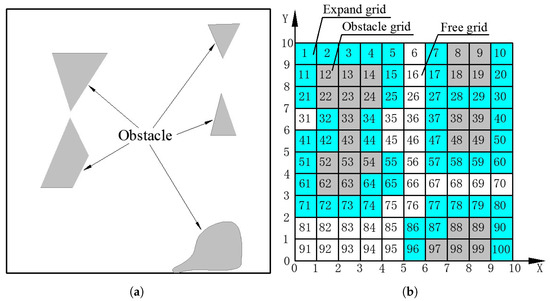
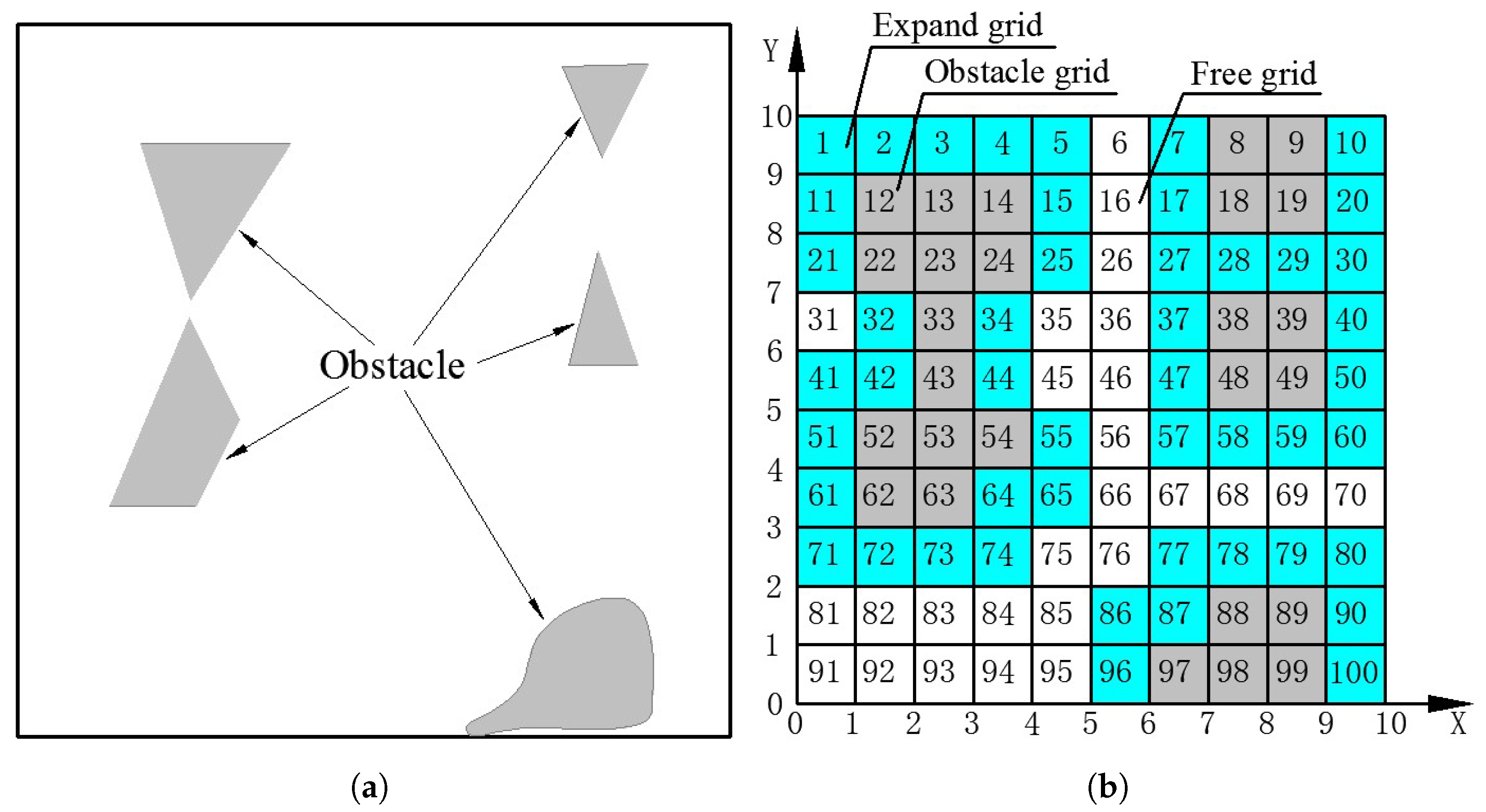
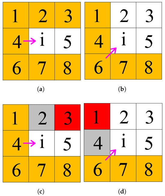
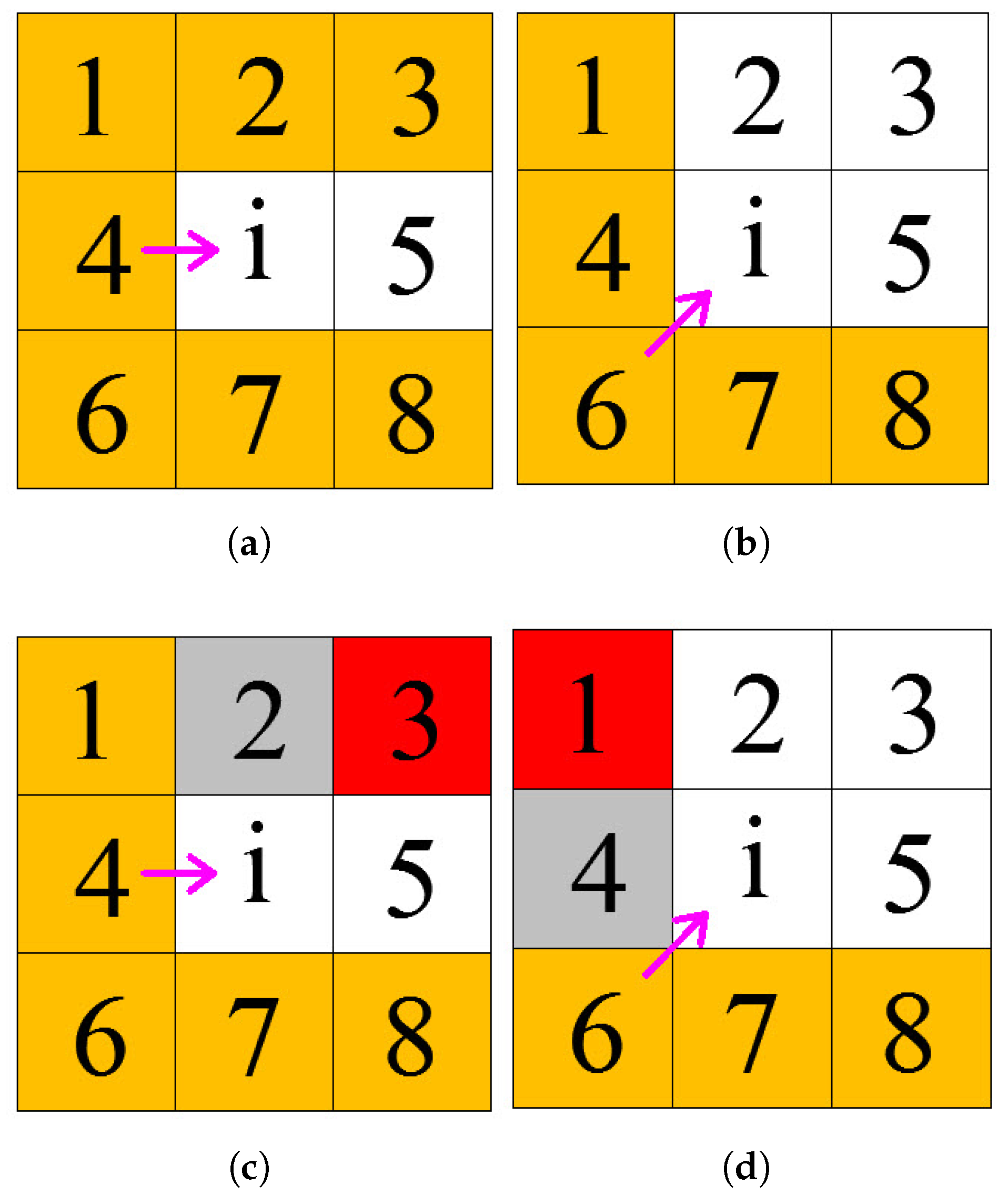
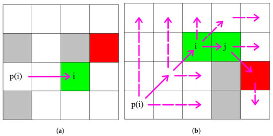
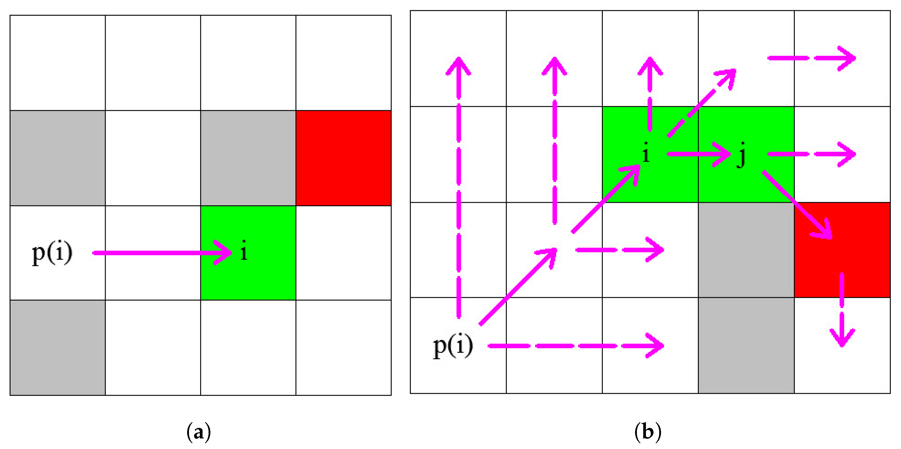
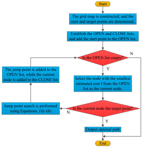
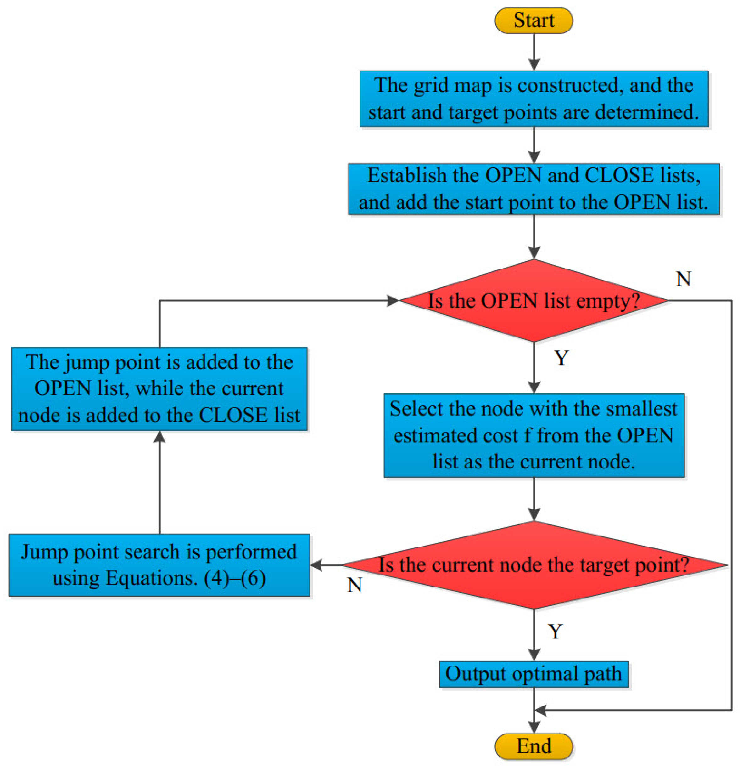
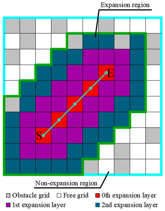
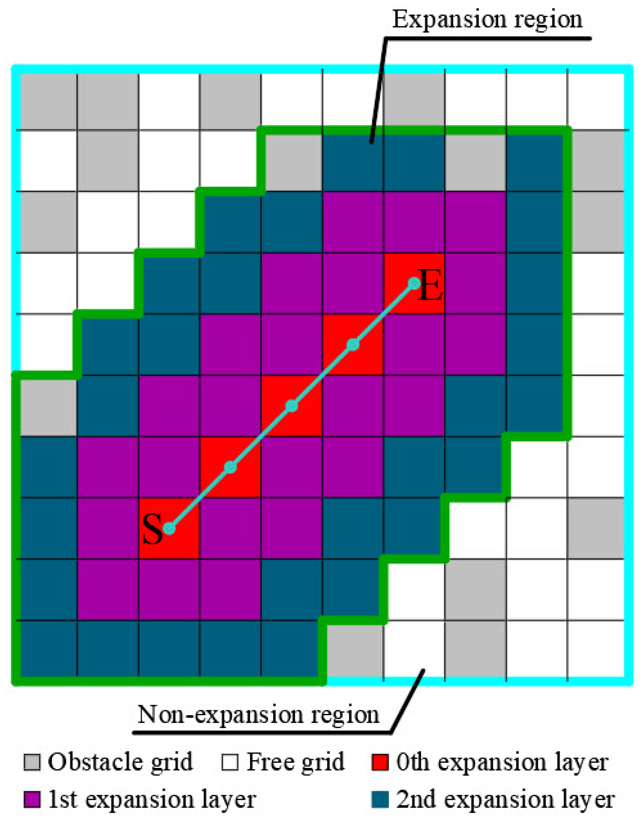
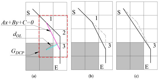
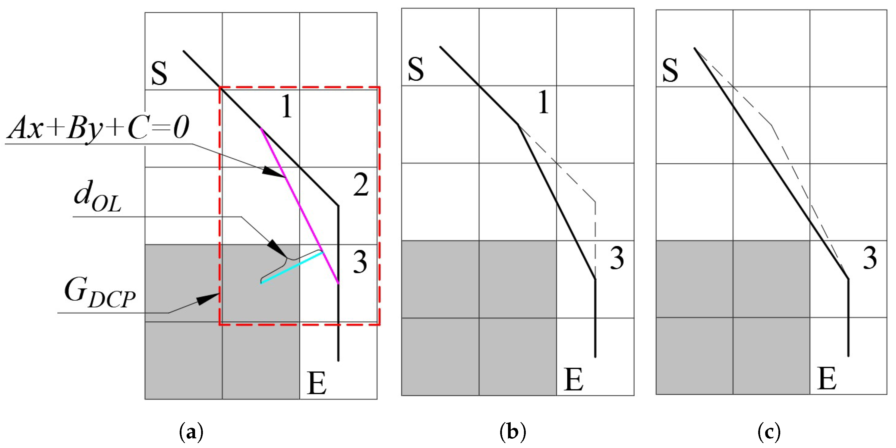
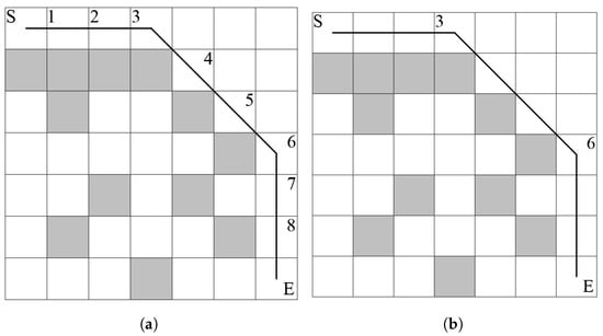
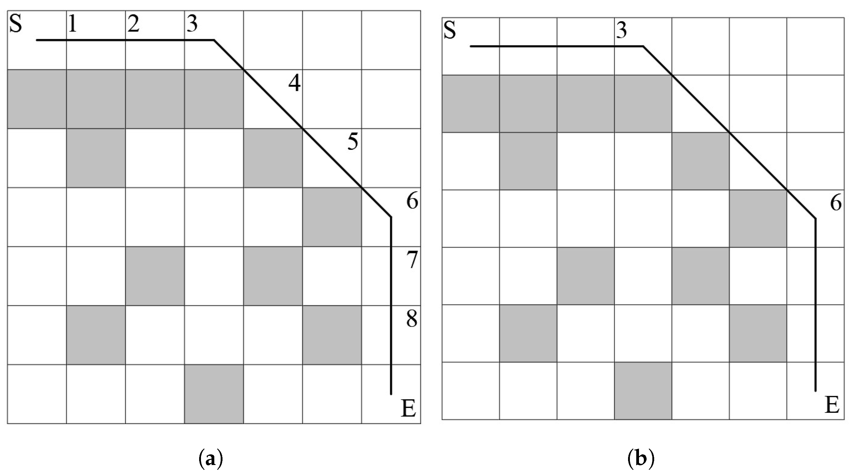
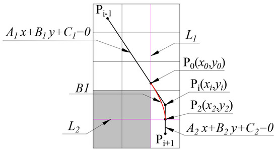
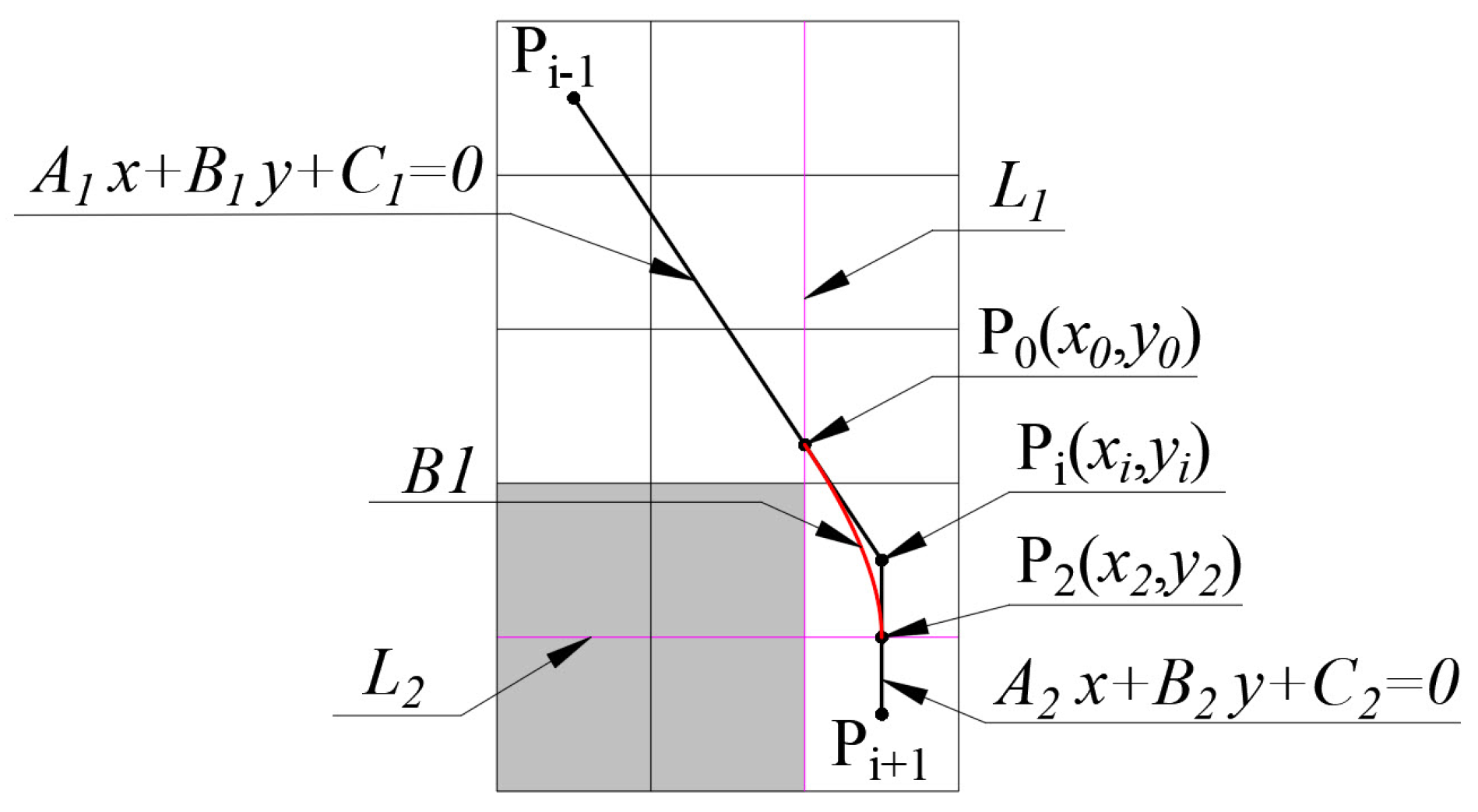
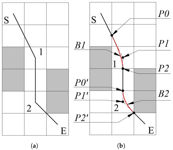
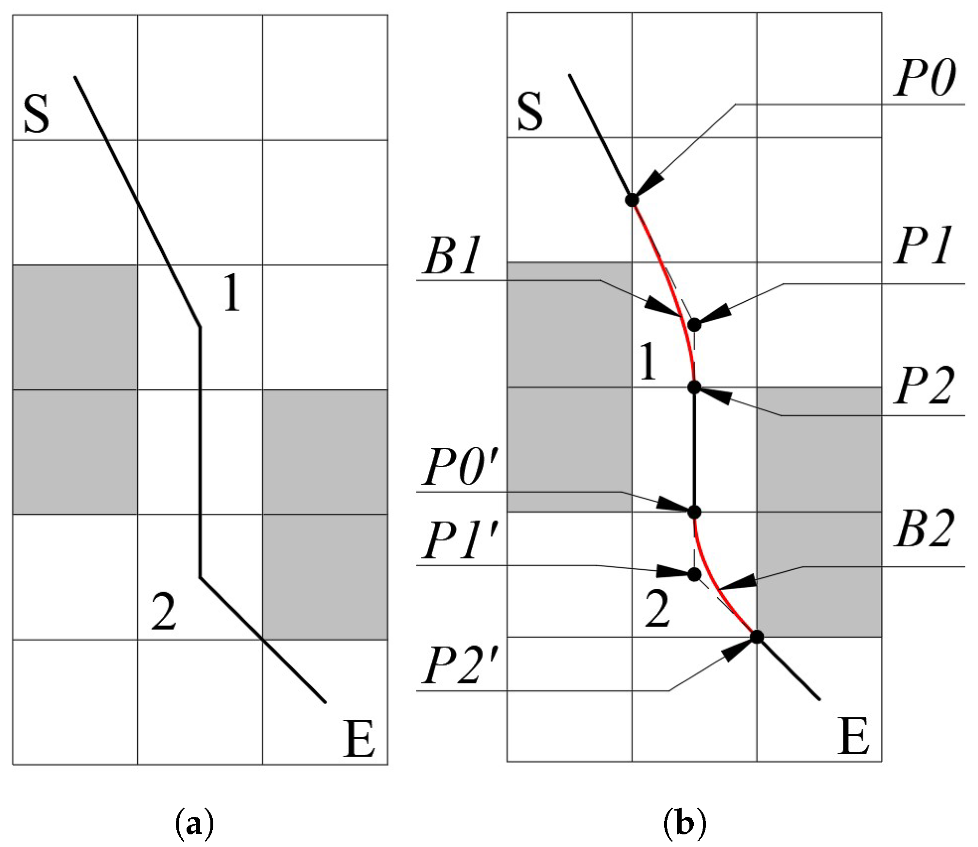
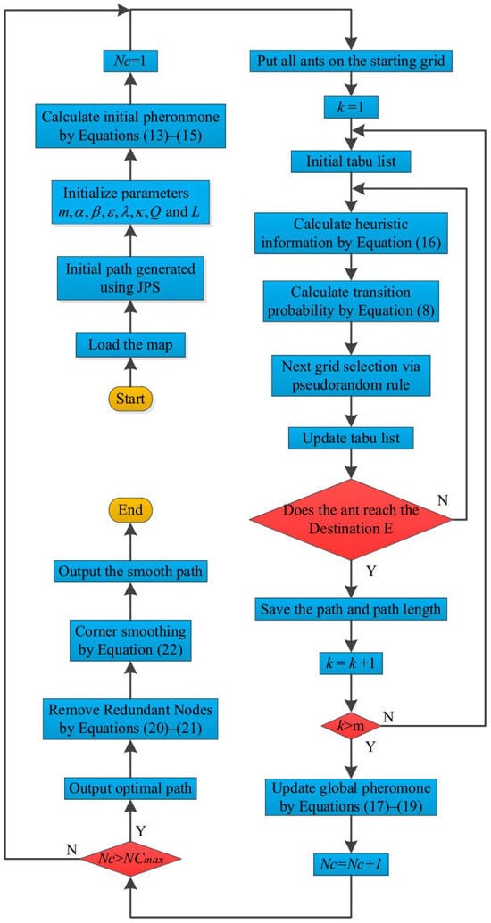
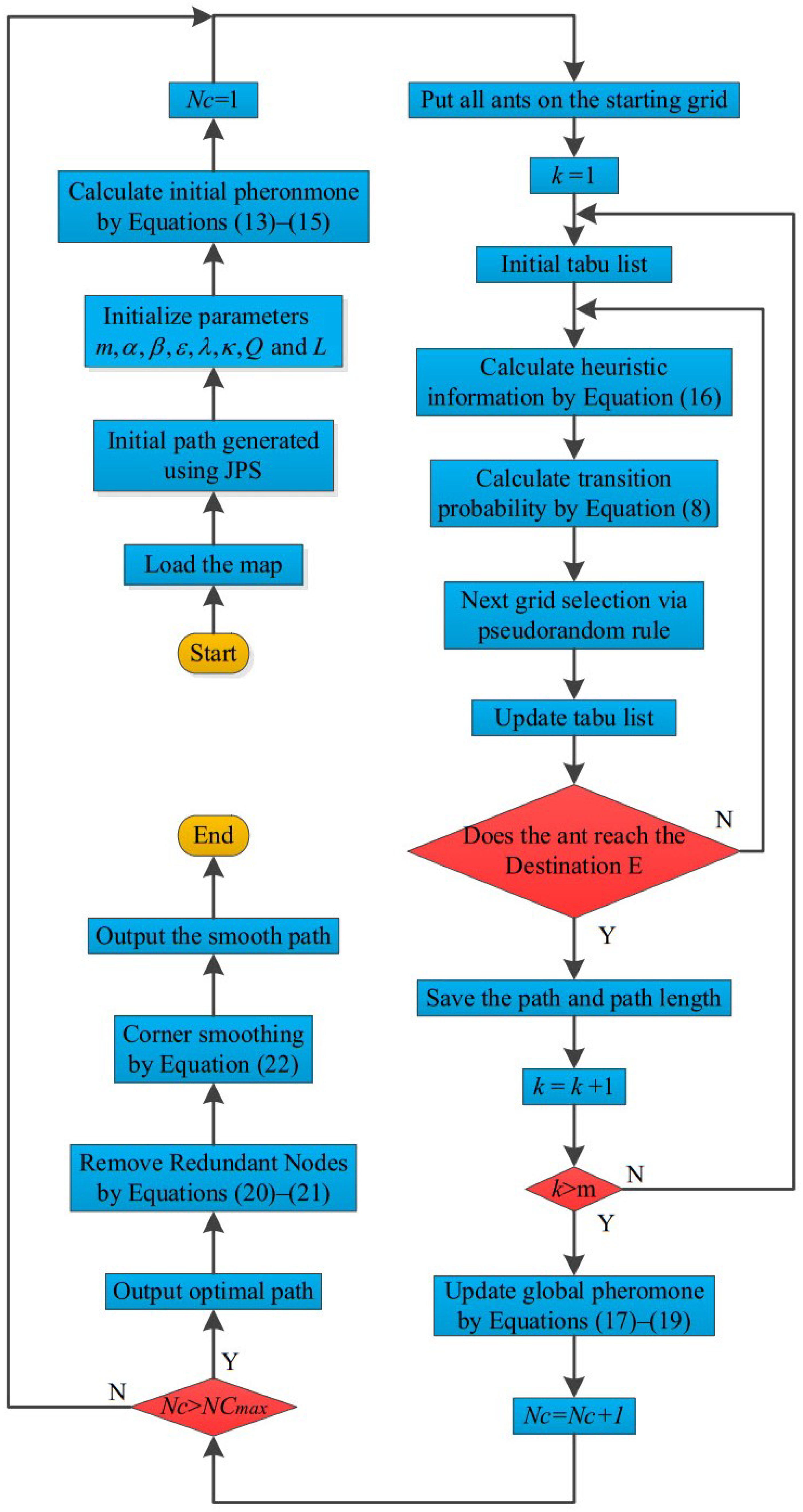
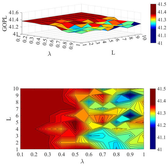
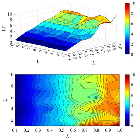
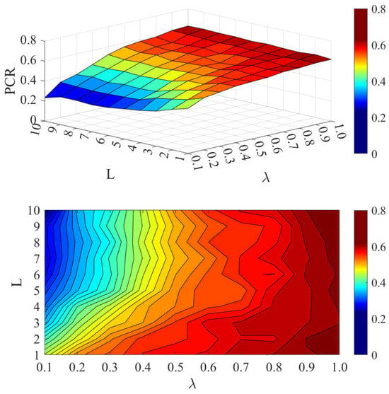
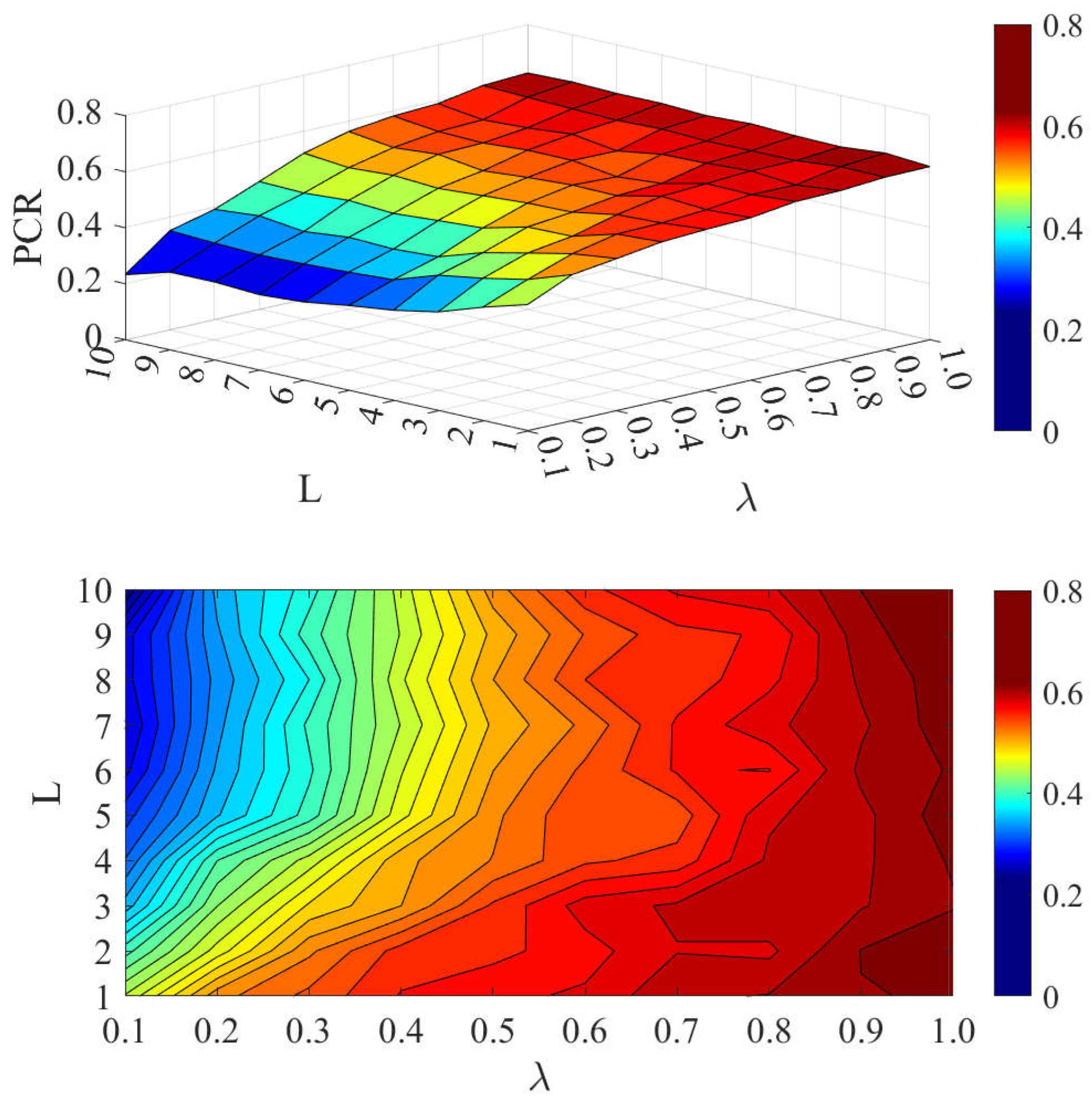
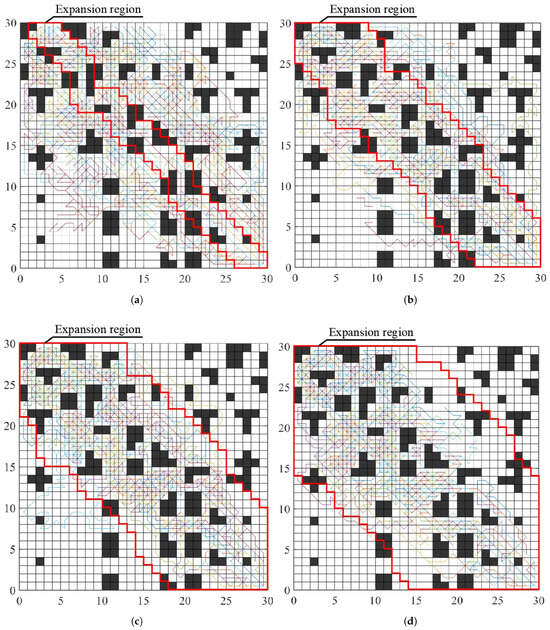
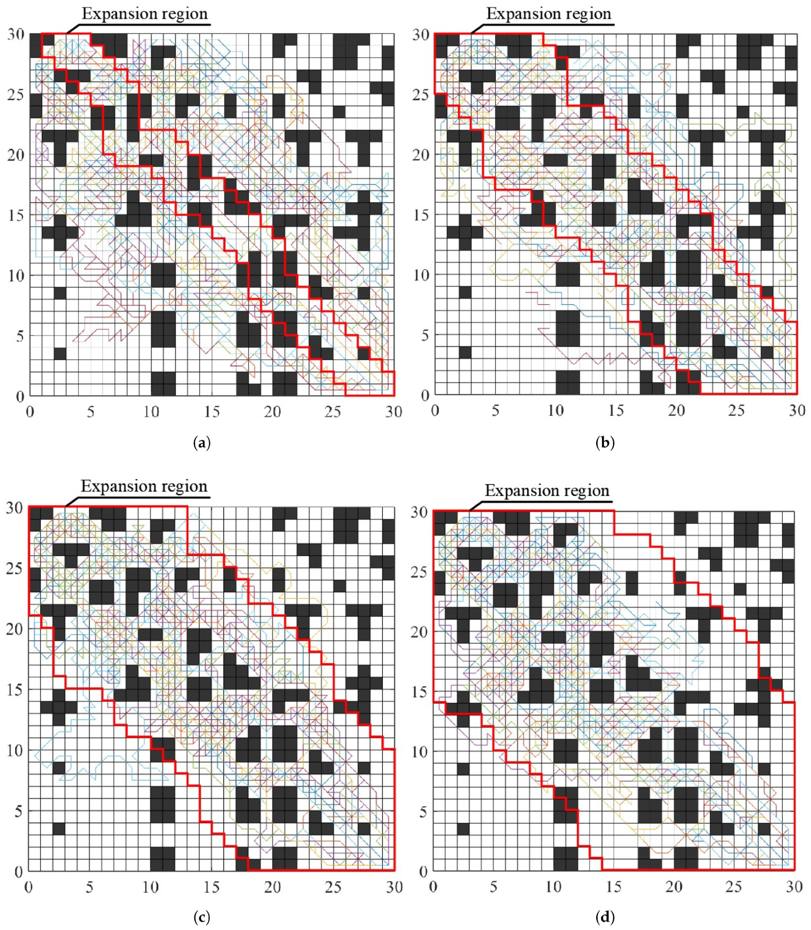
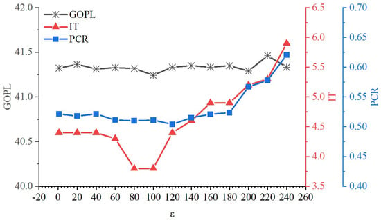
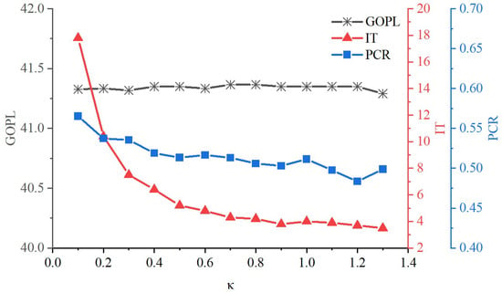
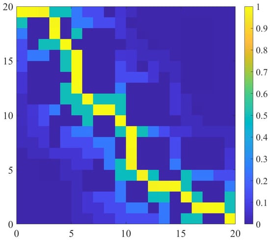
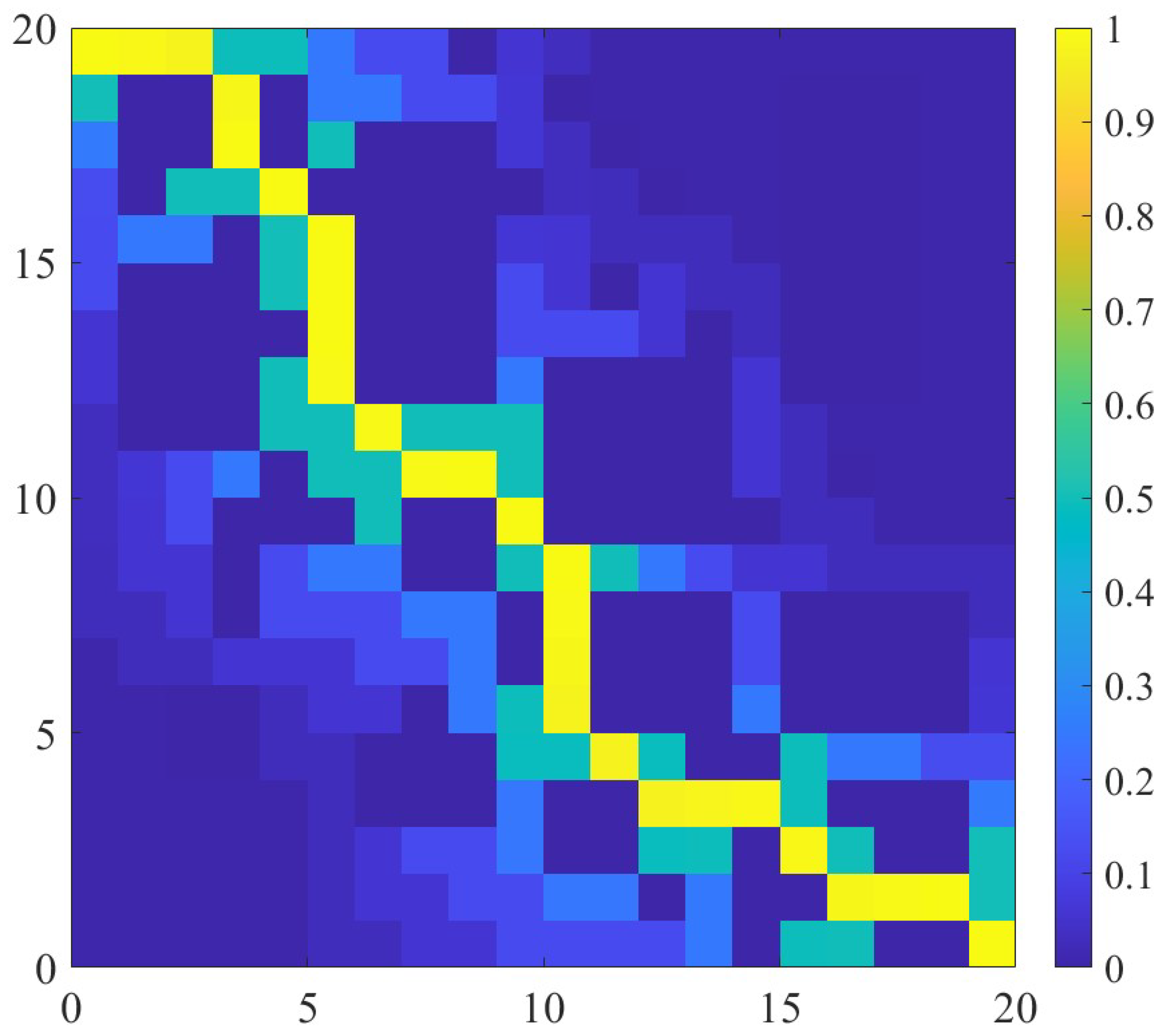
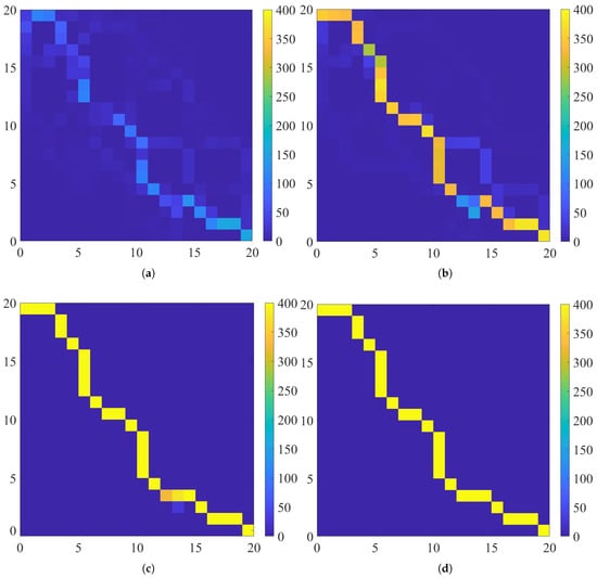
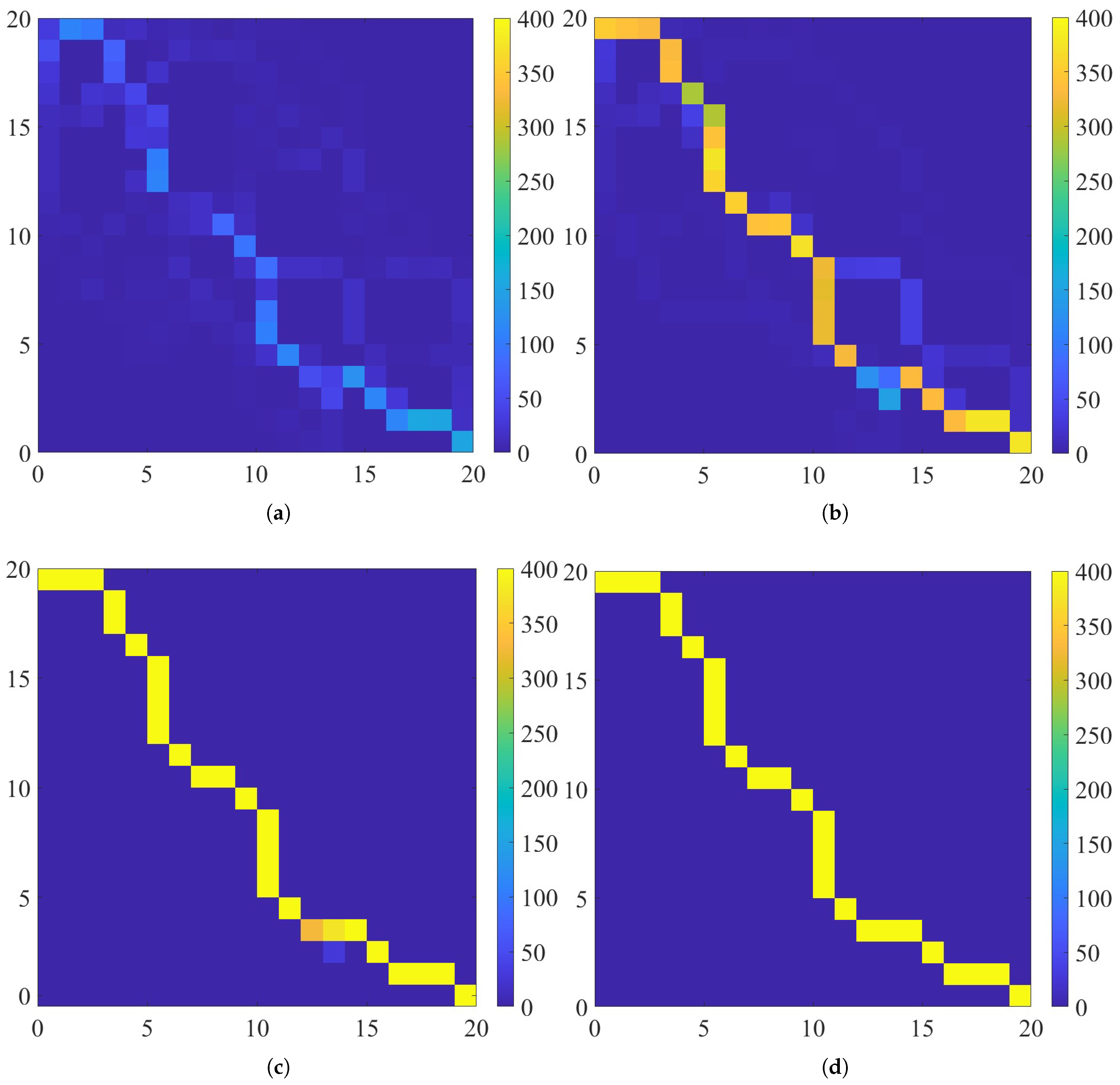
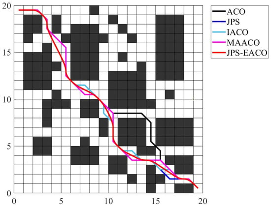
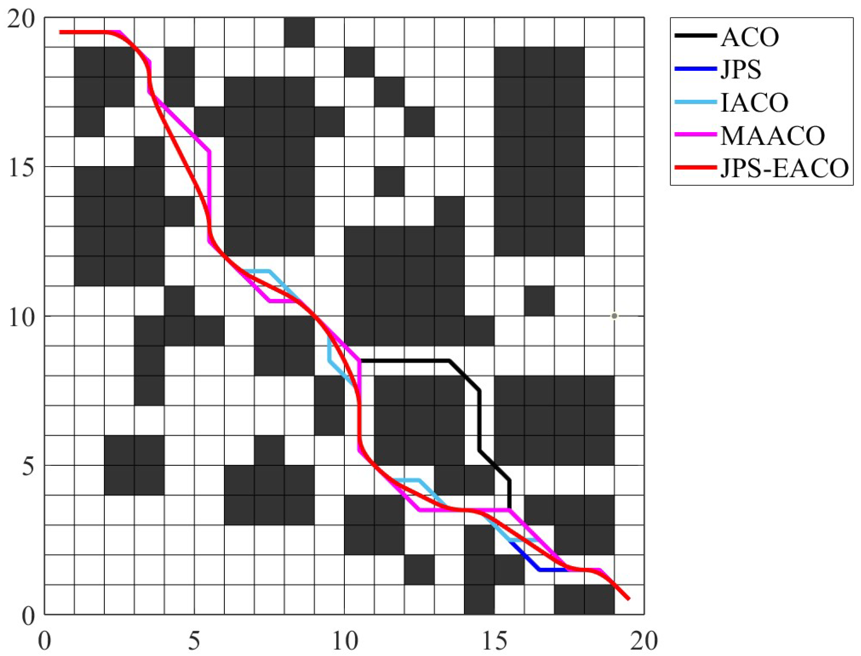
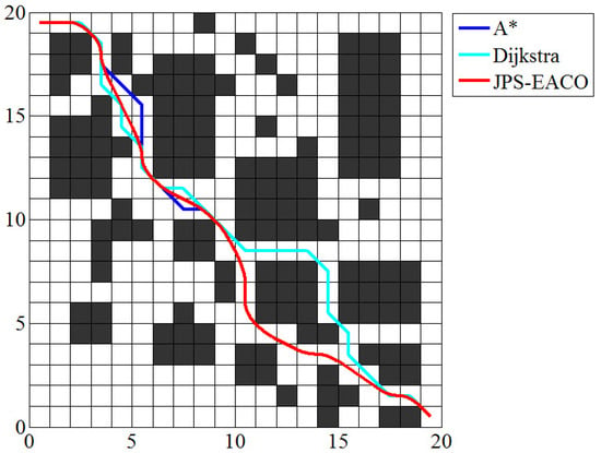
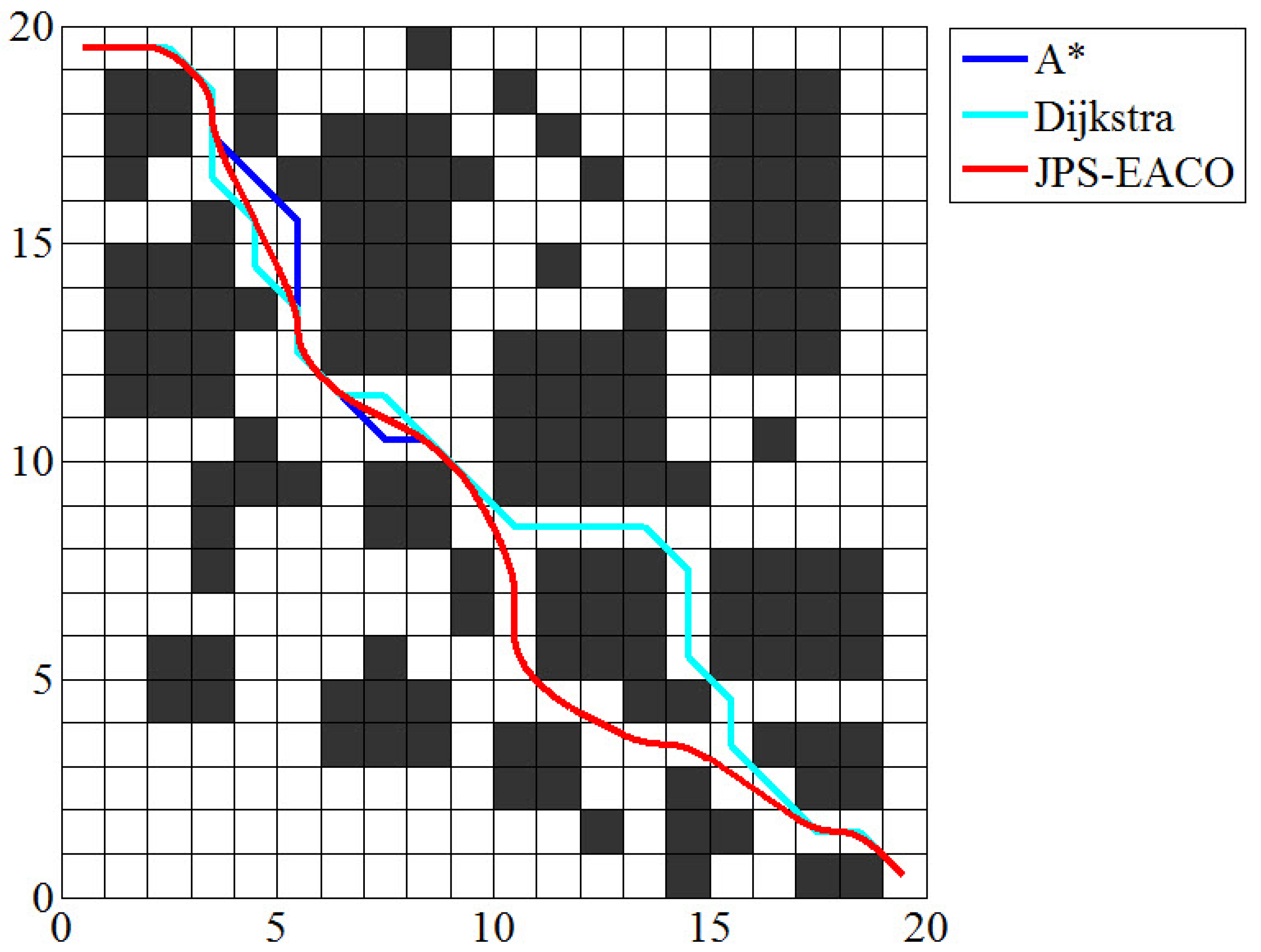
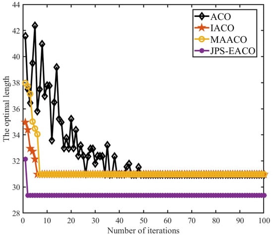
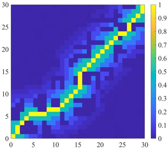
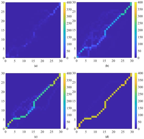
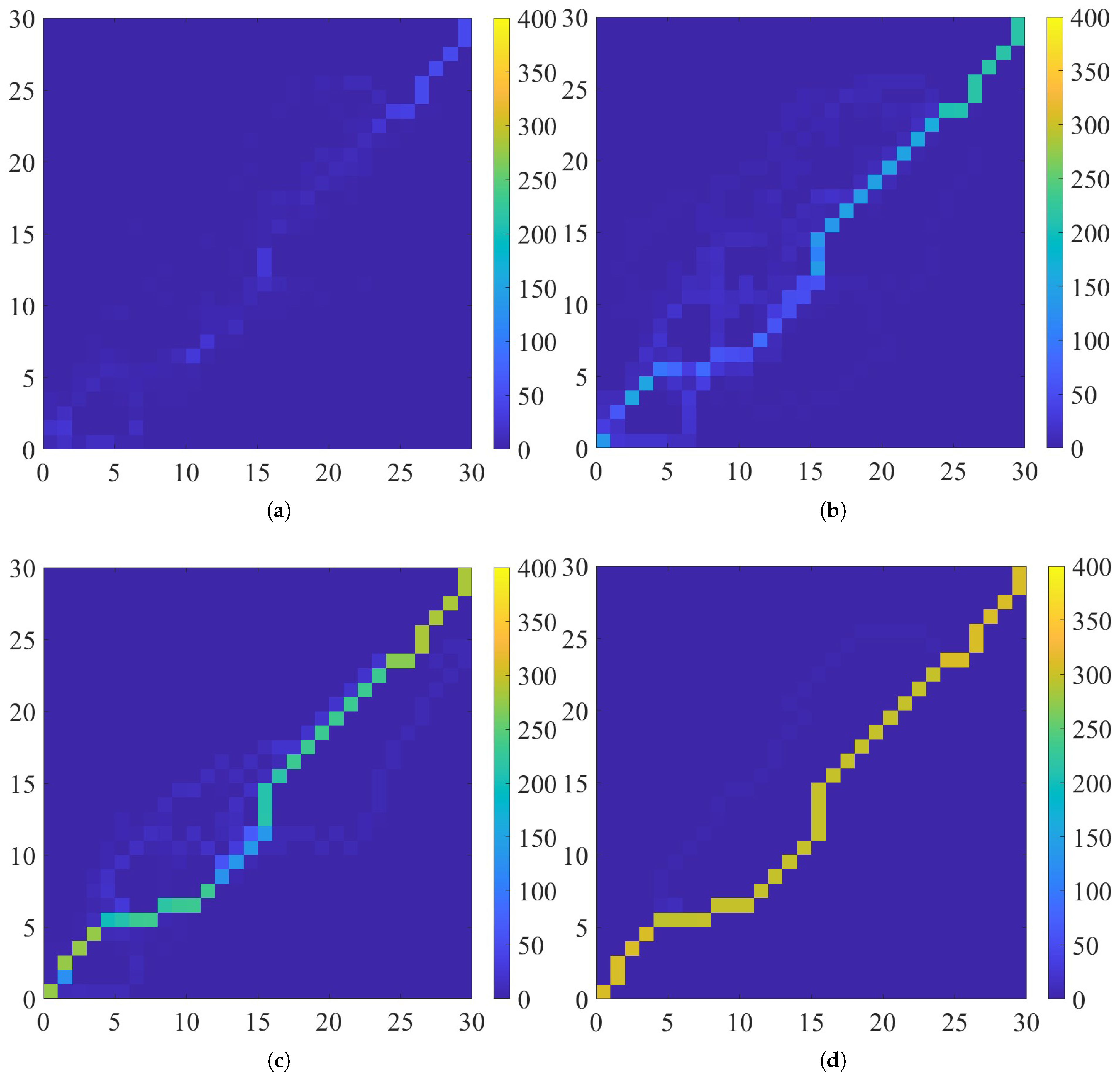
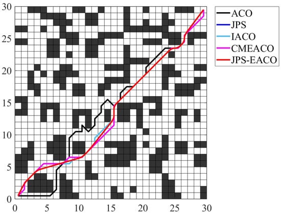
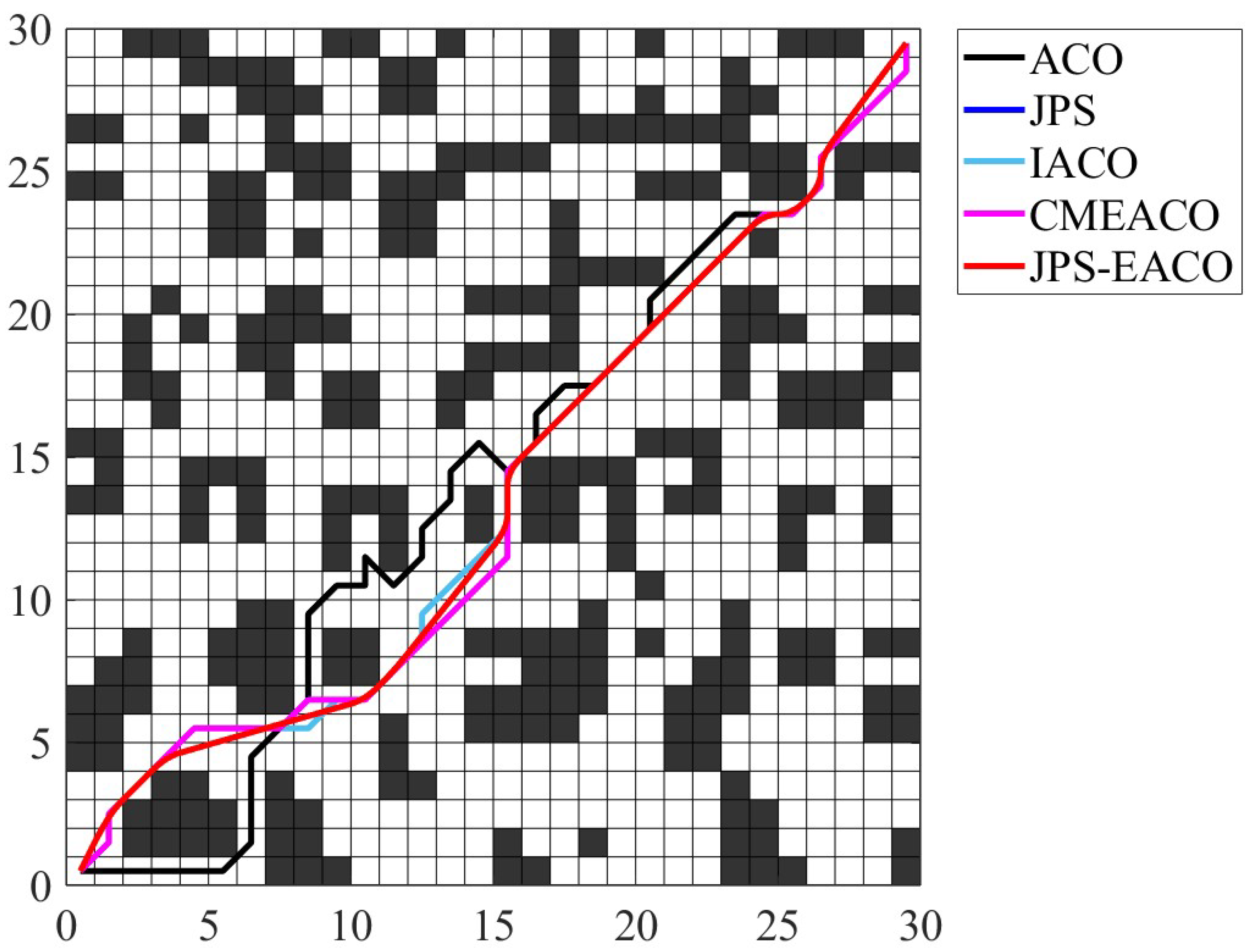
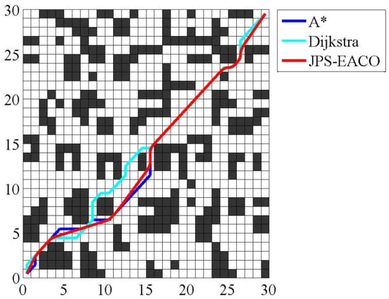
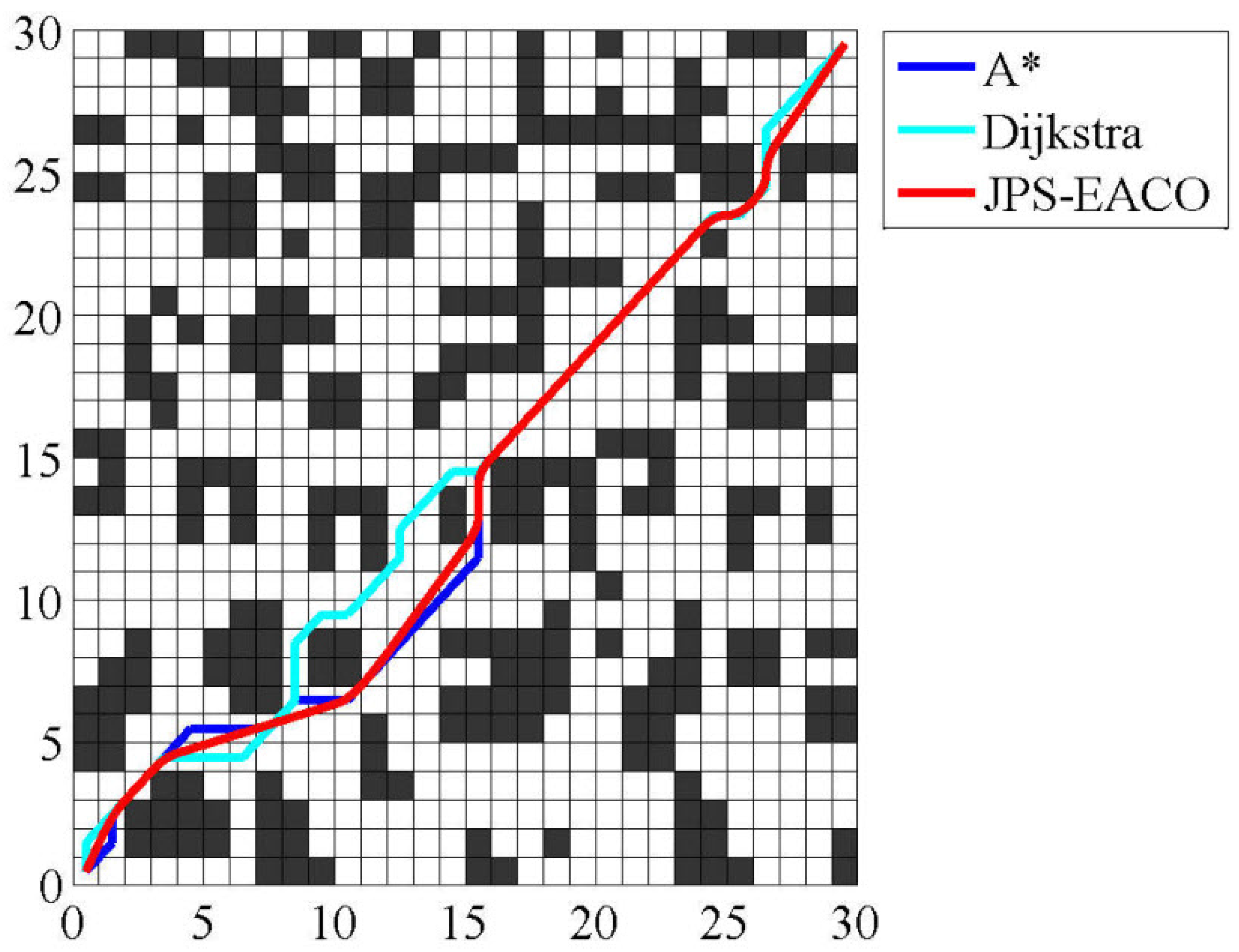
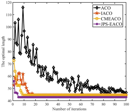
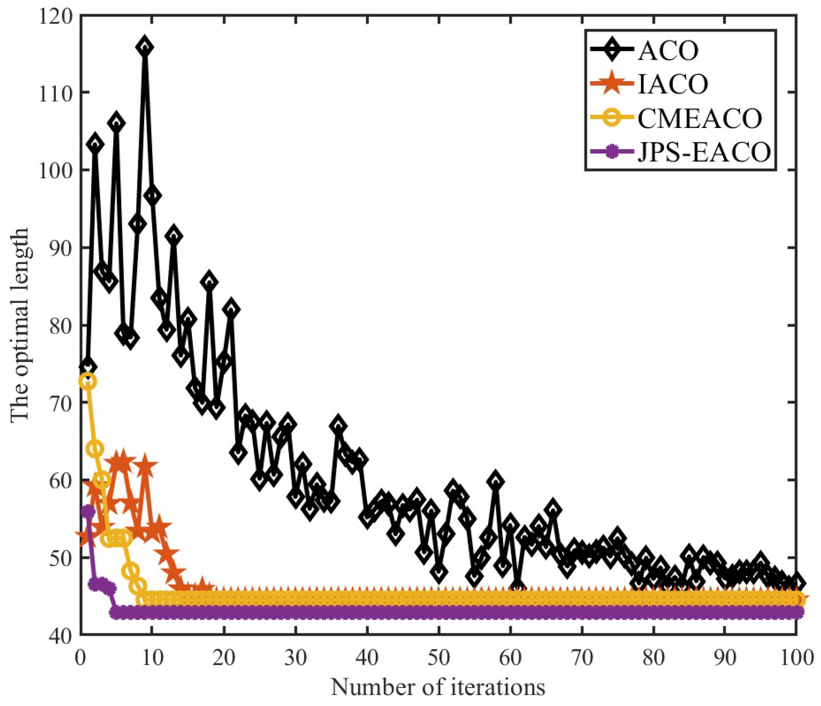
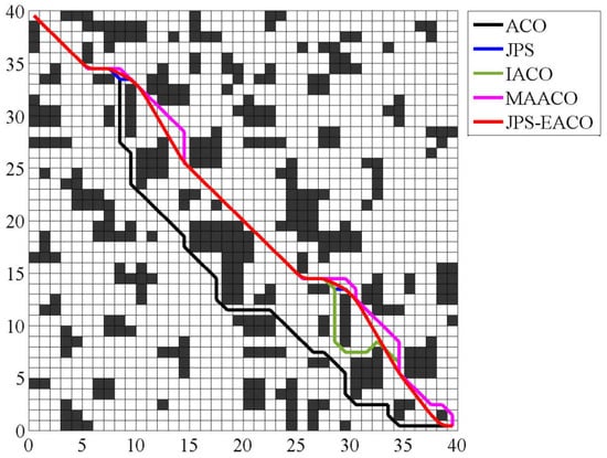
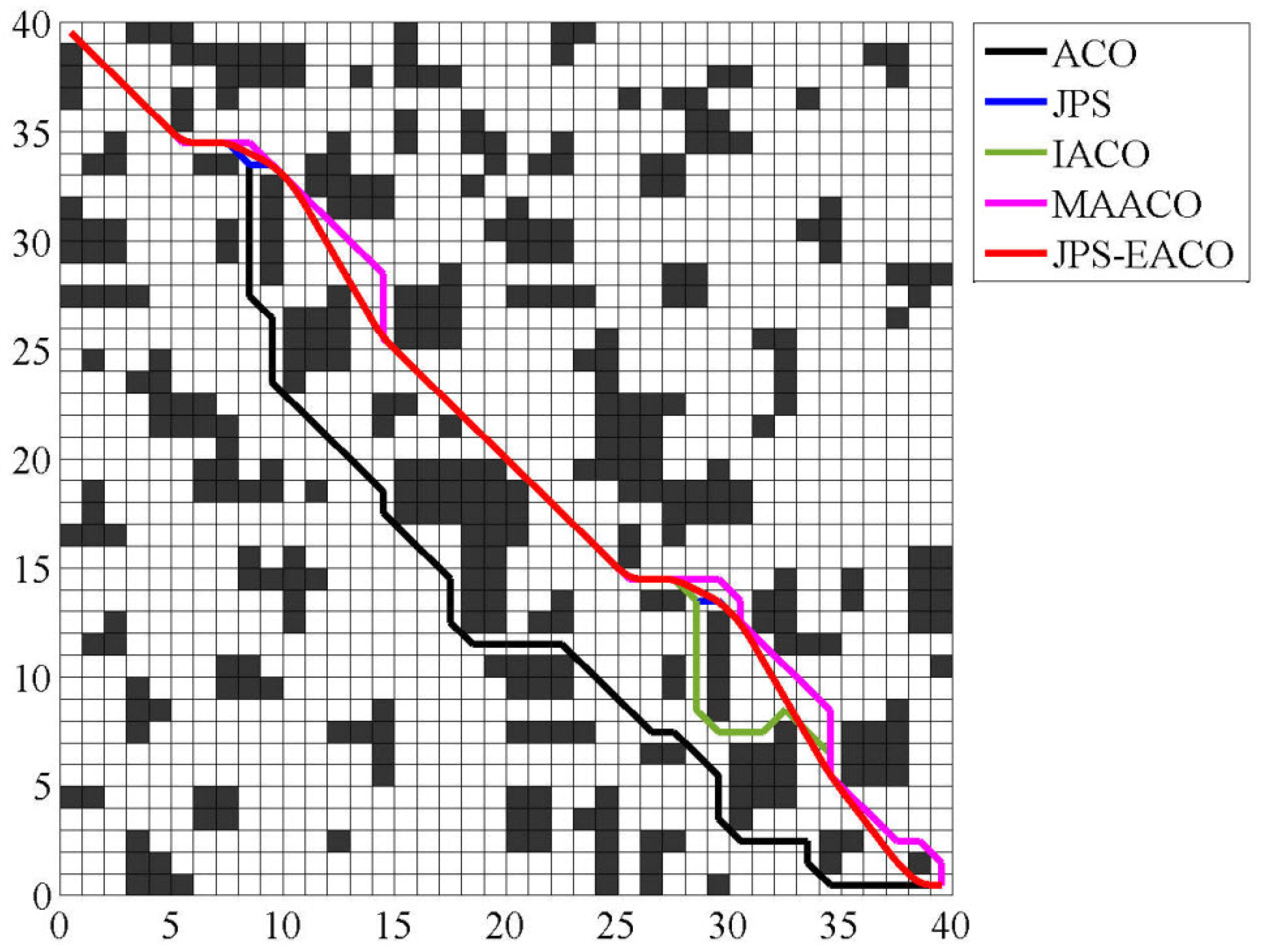
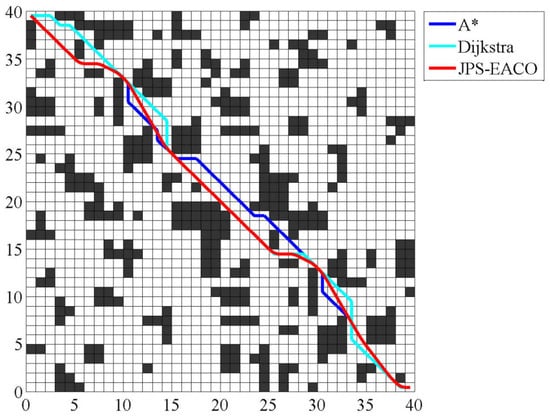
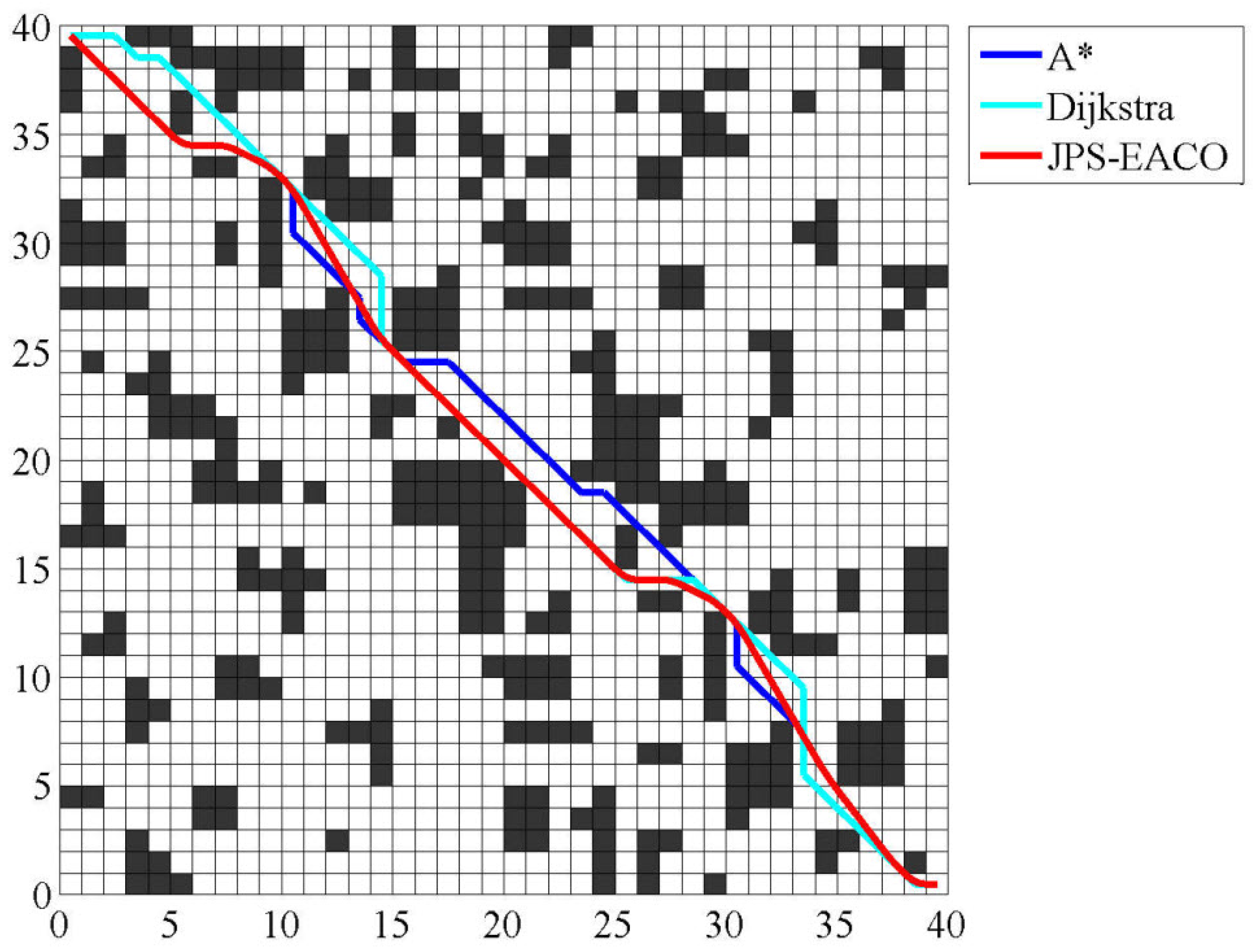
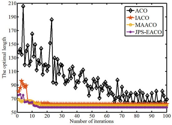
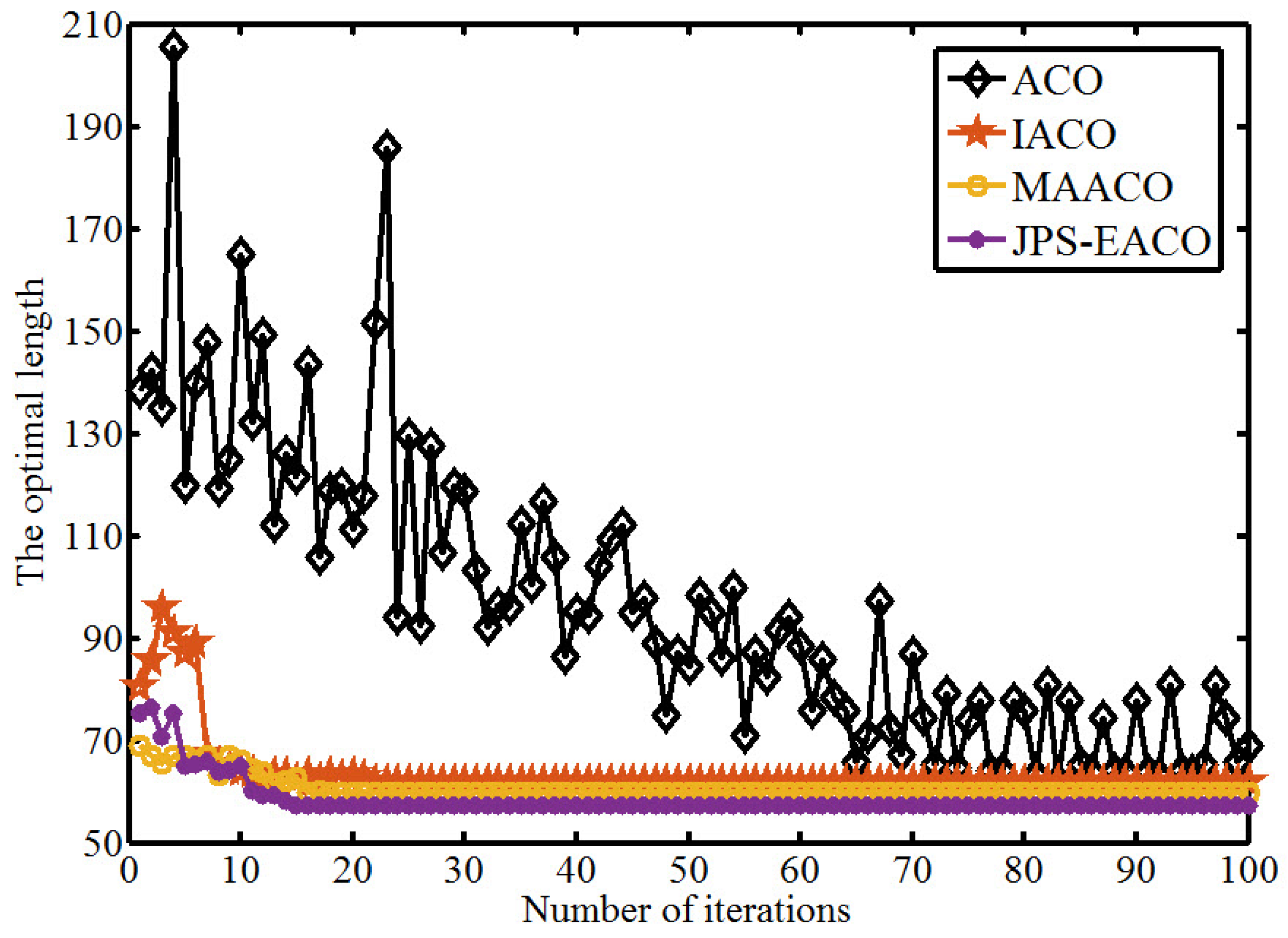
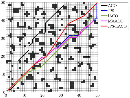
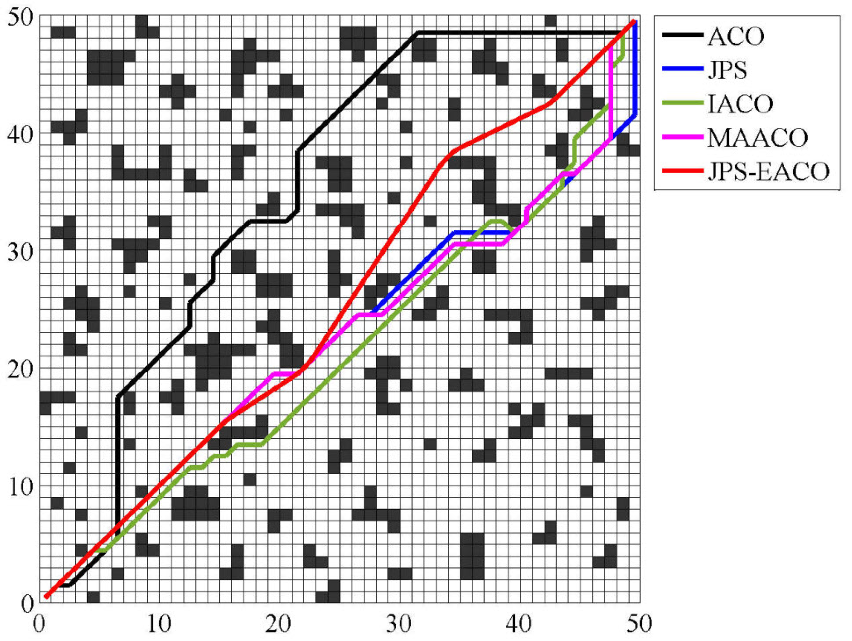
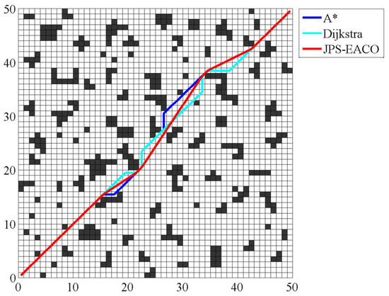
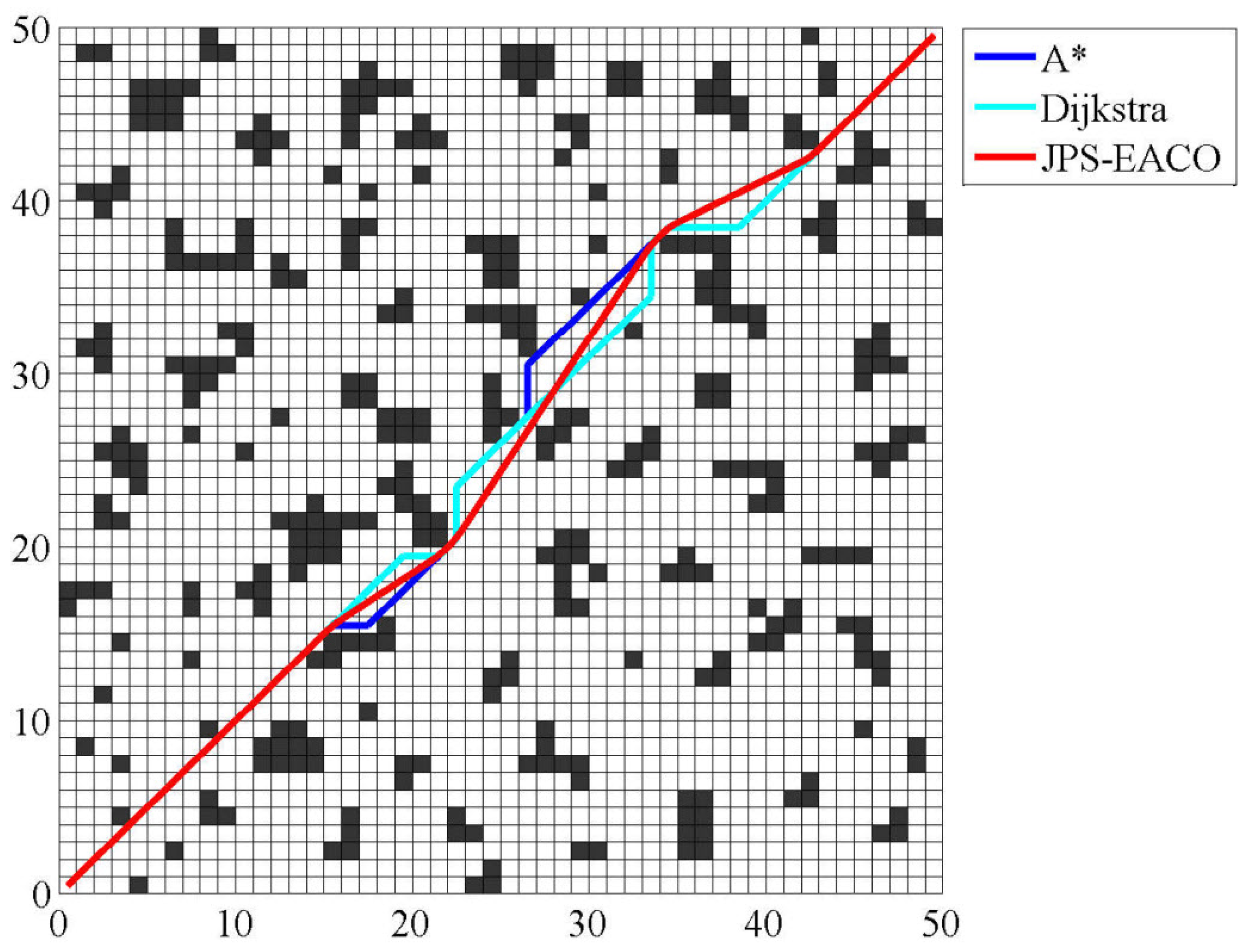
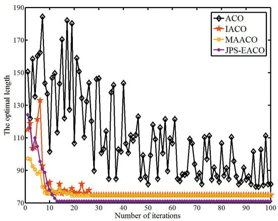
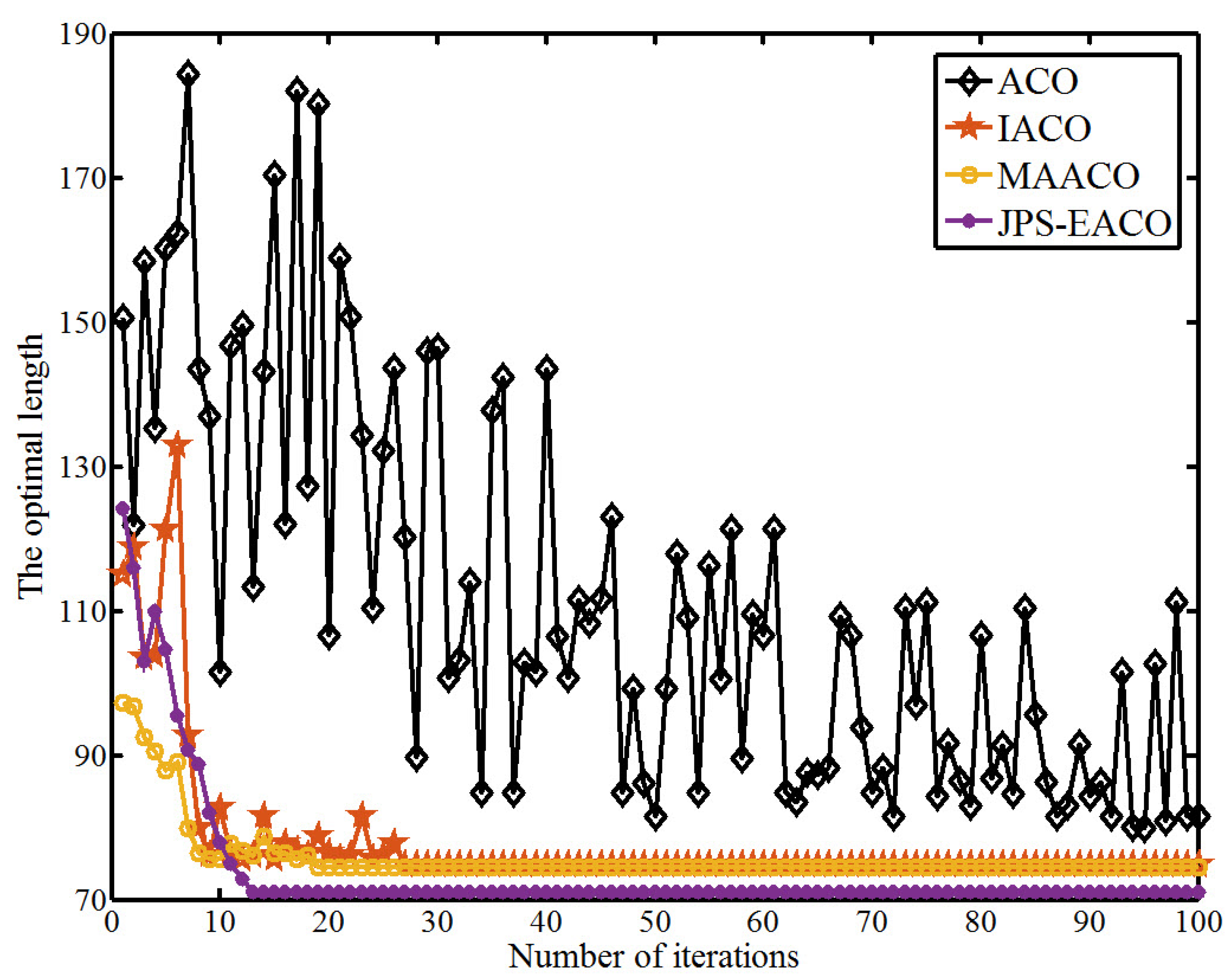
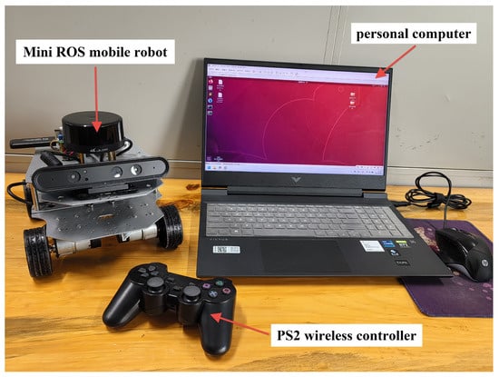
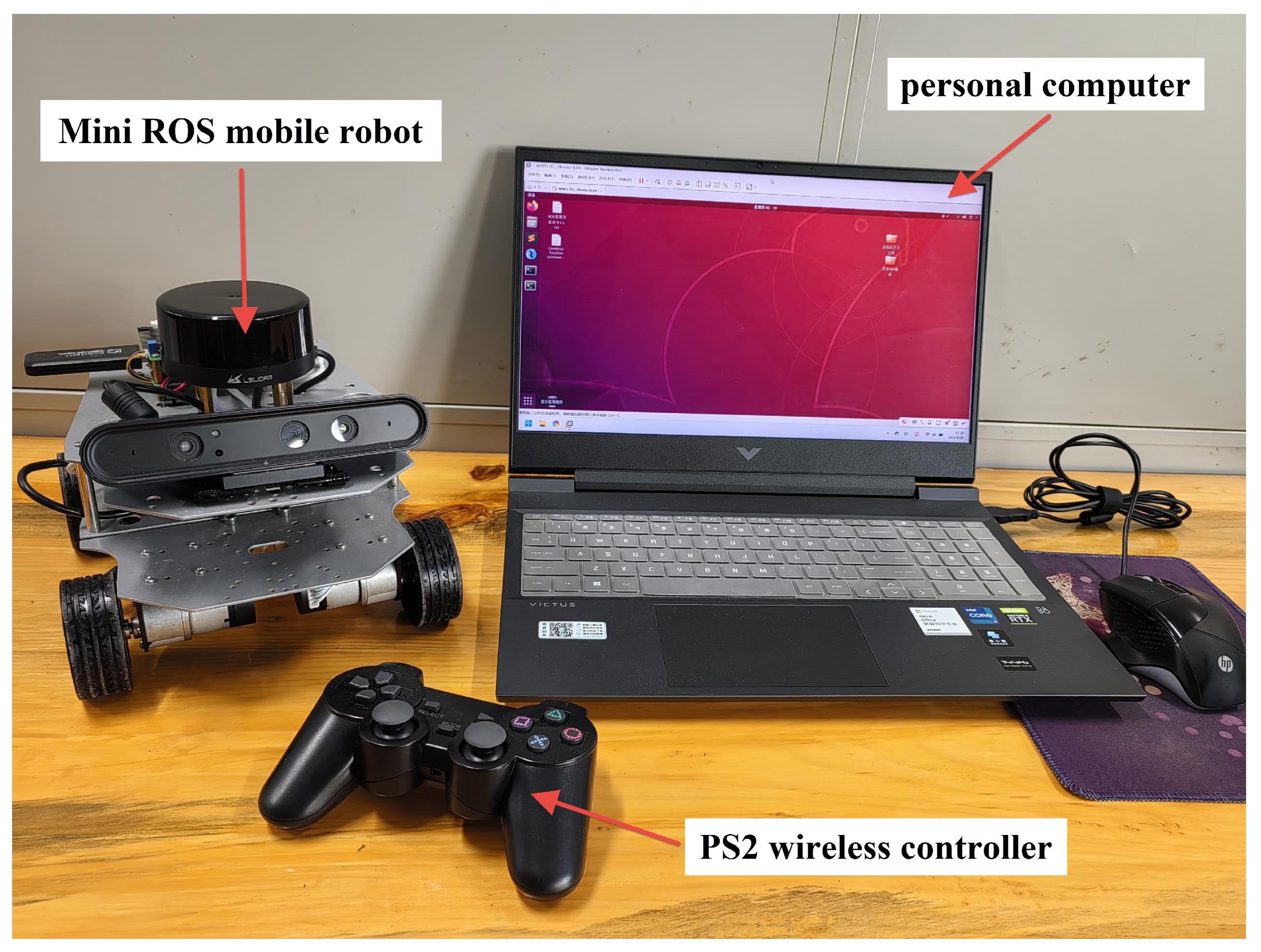
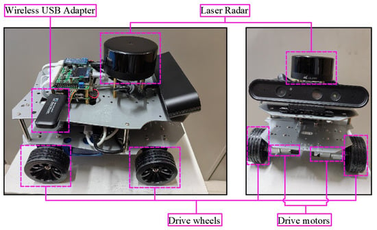
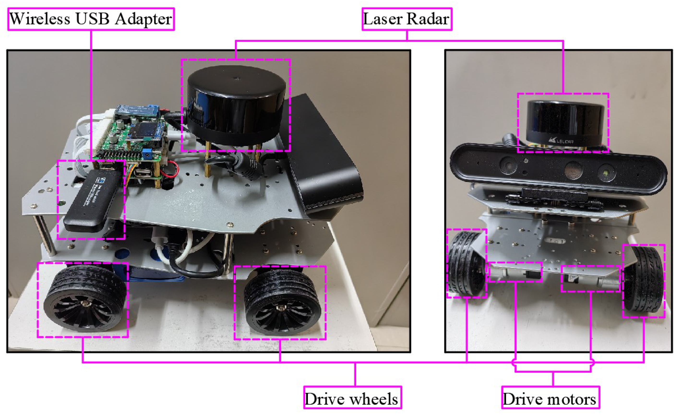
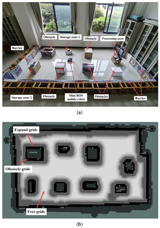
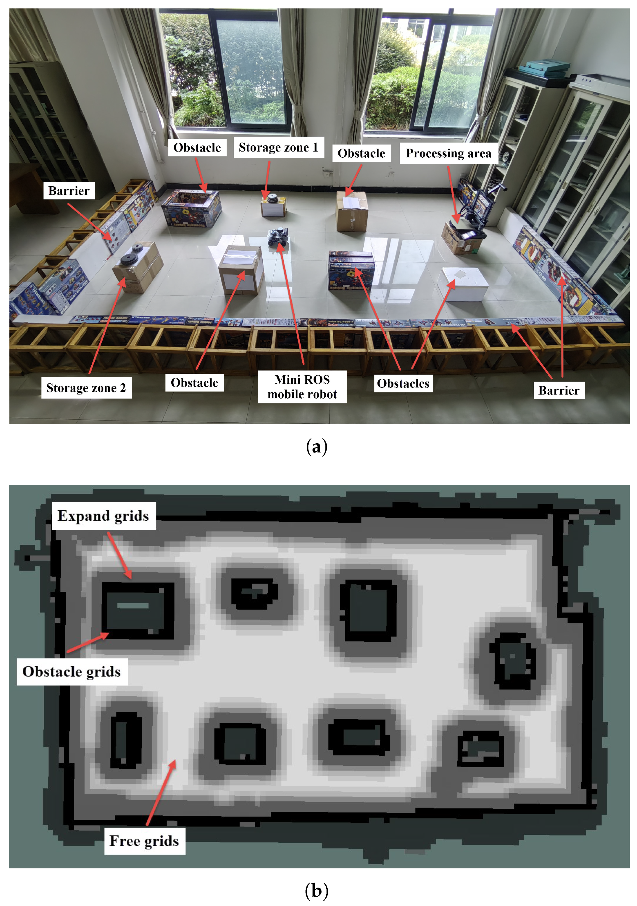
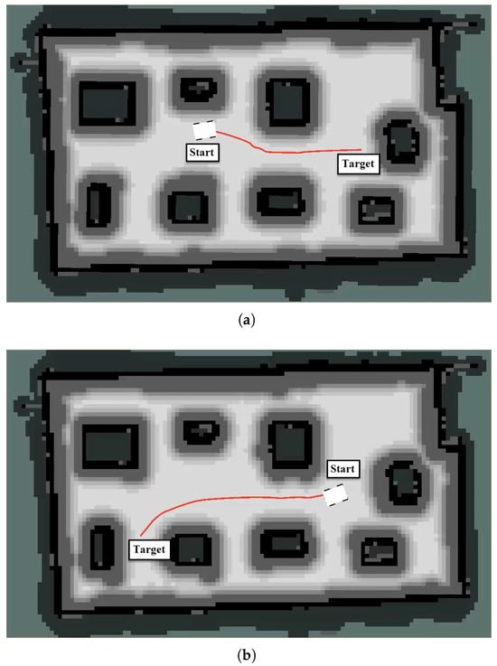
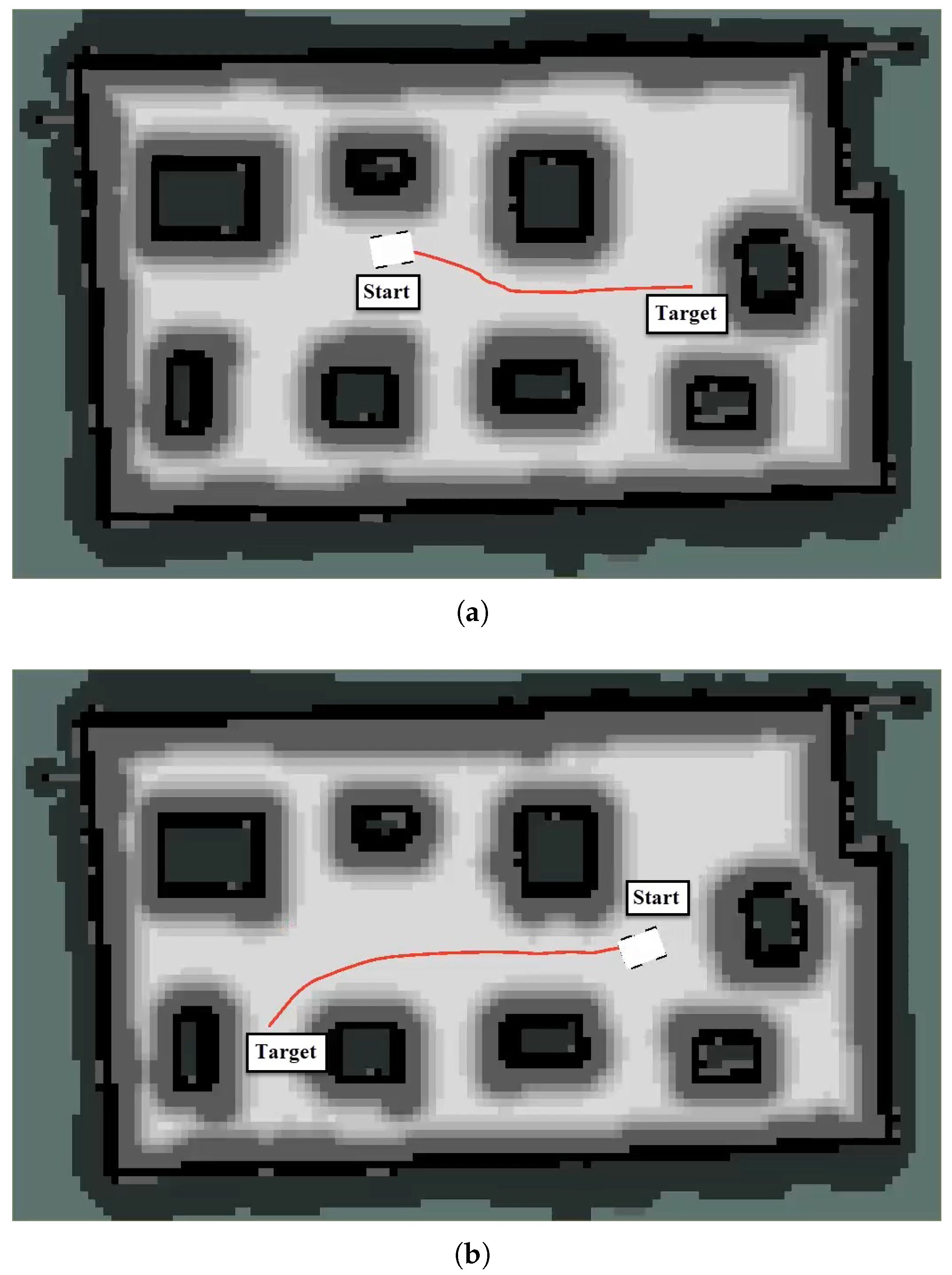

Disclaimer/Publisher’s Note: The statements, opinions and data contained in all publications are solely those of the individual author(s) and contributor(s) and not of MDPI and/or the editor(s). MDPI and/or the editor(s) disclaim responsibility for any injury to people or property resulting from any ideas, methods, instructions or products referred to in the content. |
© 2026 by the authors. Licensee MDPI, Basel, Switzerland. This article is an open access article distributed under the terms and conditions of the Creative Commons Attribution (CC BY) license.