Cross-Gradient Constrained Joint Inversion of Seismic Impedance and Resistivity

Featured Application

This work presents a cross-gradient constrained joint inversion method combining seismic wave impedance and DC resistivity data. It can be applied to near-surface geophysical investigations—such as power line route surveys, engineering site assessments, and groundwater exploration—to delineate subsurface structures and anomalous bodies with improved resolution and reliability.

Abstract

Individual geophysical inversions reflect only limited physical parameters of the subsurface and often suffer from non-uniqueness. Joint inversion of different geophysical datasets can mitigate this problem by integrating complementary information. In this study, we realize a structurally constrained joint inversion of seismic wave impedance and DC resistivity data using the cross-gradient function. The cross-gradient is discretized via the central difference quotient, and its fundamental properties are analyzed. A two-dimensional joint inversion objective function incorporating cross-gradient constraints is derived and solved using the Lagrange multiplier method. The approach relies solely on structural similarity between the two physical properties and requires no explicit petrophysical relationship. Synthetic model tests are conducted for cases where the two property distributions are structurally consistent and inconsistent, respectively. Results demonstrate that the joint inversion yields more accurate and sharper boundary delineation, geometric shapes closer to the true model, and significantly improved resolution of multiple anomalous bodies, with recovered physical property values approaching the true values and enhanced convergence speed and stability. When the two models are structurally inconsistent, the cross-gradient constraint effectively acts only on regions of common structure without introducing adverse effects or external errors elsewhere. Numerical simulations confirm the validity and reliability of the proposed algorithm in reducing inversion non-uniqueness and improving parameter accuracy.

1. Introduction

Geophysical inversion is central to geophysical exploration. Separate exploration methods, however, capture only partial information about geological bodies, and their resolution capabilities differ markedly. Field data invariably suffer from noise interference, limited coverage, and discrete sampling [1]. Consequently, inversion results often exhibit uncertainty, instability, and non-uniqueness. To overcome these inherent limitations, joint inversion of multiple geophysical datasets has become an essential strategy [2,3].

Research into geophysical joint inversion began in the 1970s. Vozoff and Jupp first jointly inverted one-dimensional direct current (DC) resistivity and magnetotelluric (MT) data [4]. During the 1980s, Raiche et al. investigated the joint inversion of transient electromagnetic (TEM) and DC resistivity data [5], while Sasaki achieved two-dimensional (2-D) joint inversion of MT and dipole–dipole resistivity data [6]. Hu Jiande addressed layered anisotropy resolution by jointly inverting TEM and DC resistivity data [7]. Dobroka et al. jointly inverted vertical seismic profiling (VSP) traveltime and surface electrical data to estimate coal seam thickness, resistivity, and velocity structure [8]. Notably, combining seismic and non-seismic data through joint inversion integrates their respective strengths and provides mutual complementarity, thereby markedly improving inversion quality. This synergy has attracted considerable attention.

Since the early 2000s, joint inversion theory and techniques have advanced rapidly. Jing Rongzhong et al. proposed a nonlinear joint inversion method based on the FasART fuzzy inference neural network [9]. Meju and Gallardo confirmed a structural similarity between near-surface resistivity and P-wave velocity and introduced the cross-gradient algorithm [10]. They successfully applied it to the 2-D joint inversion of DC resistivity sounding and seismic traveltime data [11,12] and later extended it to MT and seismic traveltime data [13]. The cross-gradient has since become a core tool for structurally coupled joint inversion. Yang Yunjian et al. discussed joint inversion strategies for AMT (audio-frequency magnetotelluric), TEM, and VES (vertical electrical sounding) data [14]. Chen Xiao et al. enhanced inversion stability by introducing Tikhonov regularization into the joint inversion framework [15].

In 2011, Moorkamp et al. performed three-dimensional (3-D) joint inversion of MT, gravity, and seismic traveltime data, comparing the applicability of direct parameter coupling versus cross-gradient constraints [16]. Peng Miao et al. developed a 3-D joint inversion algorithm for MT and seismic traveltime data under cross-gradient coupling [17]. Bennington et al. employed normalized cross-gradient constraints to jointly invert P-wave velocity and resistivity, further demonstrating the method’s advantages [18]. Gao Ji et al. proposed a strategy that decouples model updates from cross-gradient calculations, significantly simplifying implementation [19,20]. Colombo et al. compared cooperative and simultaneous joint inversion approaches for 2-D seismic traveltime and airborne electromagnetic data [21]. Shi et al. achieved 3-D cross-gradient joint inversion of seismic refraction and DC resistivity data [22]. Pak et al. developed a data-space multi-gradient joint inversion algorithm [23]. Zhang Rongzhe et al. completed a 2-D cross-gradient joint inversion of gravity, magnetic, electrical, and seismic data [24]. Yin Changchun et al. proposed a joint inversion method constrained by the local Pearson correlation coefficient, which improved convergence and mitigated non-uniqueness [25].

More recently, deep learning techniques have entered the field of joint inversion. Li Fei et al. combined a convolutional neural network (CNN) with a long short-term memory (LSTM) network for joint inversion of mine TEM and seismic data [26]. Yan Zhengwen et al. optimized 3-D joint inversion of gravity, magnetic, and electrical data using cross-gradients and deep learning networks [27]. Zhang Zhihou et al. designed GraInvNet, a deep learning network for joint inversion of gravity and gravity gradiometry data [28]. He Haoyuan et al. implemented 3-D joint inversion of gravity, gravity gradiometry, and MT data using smoothing focusing regularization and cross-gradients [29]. Liu Jiacheng et al. introduced fuzzy c-means (FCM) clustering constraints to the joint inversion of DC resistivity and seismic traveltime tomography data [30]. Wang Liang et al. developed a deep learning joint inversion network for audio-frequency MT and TEM data [31]. Kong Fanxiang et al. applied cross-gradients to achieve a 2-D joint inversion of marine controlled-source electromagnetic (CSEM) data and seismic full-waveform inversion (FWI) data [32]. Zhang et al. proposed an integration method of elastic neural network full-waveform inversion and rock physics framework [33]. Penta de Peppo et al. developed a structured grid cross-gradient joint inversion approach for ERT and seismic refraction data over rugged topography [34].

In summary, joint inversion can be classified by data type—into inversion of the same versus different physical property parameters—and by implementation approach—into methods based on prior petrophysical relationships versus those based on structural similarity constraints. This study combines DC resistivity and seismic wave impedance data. Unlike previous cross-gradient studies that primarily focused on joint inversion of resistivity (or MT) with seismic traveltime data, this study introduces cross-gradient constraints into the joint inversion of wave impedance and DC resistivity data—a combination that offers unique applicability in medium-to-shallow engineering exploration and can be readily extended to other seismic methods such as microtremor and surface wave techniques. First, we perform wave impedance inversion on the seismic data to obtain an initial model. We then use the preliminary resistivity inversion result as the starting model and introduce cross-gradient constraints to perform joint inversion. The resulting resistivity model not only delineates structural distribution with improved resolution but also effectively assesses water-bearing conditions within the structures.

2. Materials and Methods

2.1. Cross-Gradient Constraint Function

One may measure structural differences between seismic wave impedance and resistivity inversion results using an angle function—for example

$${\mathsf{\theta }(\mathrm{x},\mathrm{y},\mathrm{z})=\cos }^{-1}\left({\displaystyle \frac{\nabla {\mathrm{m}}_{\mathrm{r}}(\mathrm{x},\mathrm{y},\mathrm{z})\cdot \nabla {\mathrm{m}}_{\mathrm{s}}(\mathrm{x},\mathrm{y},\mathrm{z})}{|\nabla {\mathrm{m}}_{\mathrm{r}}(\mathrm{x},\mathrm{y},\mathrm{z})\left|\right|\nabla {\mathrm{m}}_{\mathrm{s}}(\mathrm{x},\mathrm{y},\mathrm{z})|}}\right)$$

(1)

or a correlation function—for example, $1/(1-\cos \mathsf{\theta })$. These nonlinear functions exhibit discontinuity at points where $\nabla {\mathrm{m}}_{\mathrm{r}}(\mathrm{x},\mathrm{y},\mathrm{z})$ or $\nabla {\mathrm{m}}_{\mathrm{s}}(\mathrm{x},\mathrm{y},\mathrm{z})$ equals zero (e.g., in uniform media or where local maxima or minima exist). We therefore adopt the cross-gradient function, defined as

$$\overrightarrow{\mathsf{\tau }} (\mathrm{x},\mathrm{y},\mathrm{z})=\nabla {\mathrm{m}}_{\mathrm{r}}(\mathrm{x},\mathrm{y},\mathrm{z})\times \nabla {\mathrm{m}}_{\mathrm{s}}(\mathrm{x},\mathrm{y},\mathrm{z})$$

(2)

In the two-dimensional case, with the strike direction set as the y-axis, the cross-gradient equals the cross product of the resistivity gradient and the wave impedance gradient. In 2-D, the cross-gradient has only a component along the strike direction, and its magnitude is

$$\begin{array}{ll}\mathsf{\tau }(\mathsf{\rho },\mathrm{k})& =\nabla {\mathrm{m}}_{\mathrm{r}}(\mathrm{x},\mathrm{z})\times \nabla {\mathrm{m}}_{\mathrm{s}}(\mathrm{x},\mathrm{z})\\ & =({\displaystyle \frac{\mathsf{\partial }{\mathrm{m}}_{\mathrm{r}}(\mathrm{x},\mathrm{z})}{\mathsf{\partial }\mathrm{z}}})({\displaystyle \frac{\mathsf{\partial }{\mathrm{m}}_{\mathrm{s}}(\mathrm{x},\mathrm{z})}{\mathsf{\partial }\mathrm{x}}})-({\displaystyle \frac{\mathsf{\partial }{\mathrm{m}}_{\mathrm{r}}(\mathrm{x},\mathrm{z})}{\mathsf{\partial }\mathrm{x}}})({\displaystyle \frac{\mathsf{\partial }{\mathrm{m}}_{\mathrm{s}}(\mathrm{x},\mathrm{z})}{\mathsf{\partial }\mathrm{z}}})\end{array}$$

(3)

For the cross-gradient function, if $\mathsf{\tau }(\mathsf{\rho },\mathrm{k})=0$ holds at every location, it indicates that the resistivity and seismic model exhibit identical variation directions throughout, meaning they share the same structural configuration.

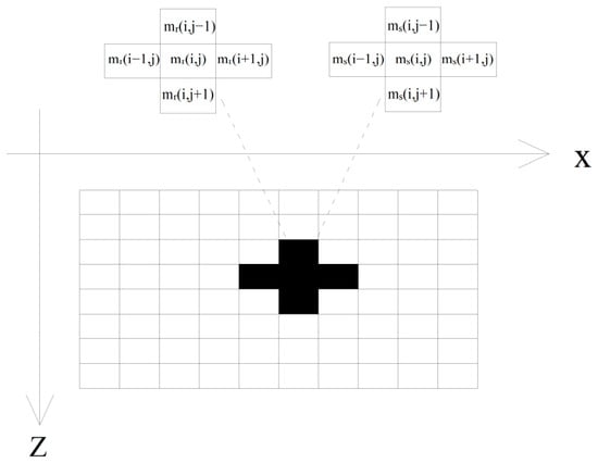
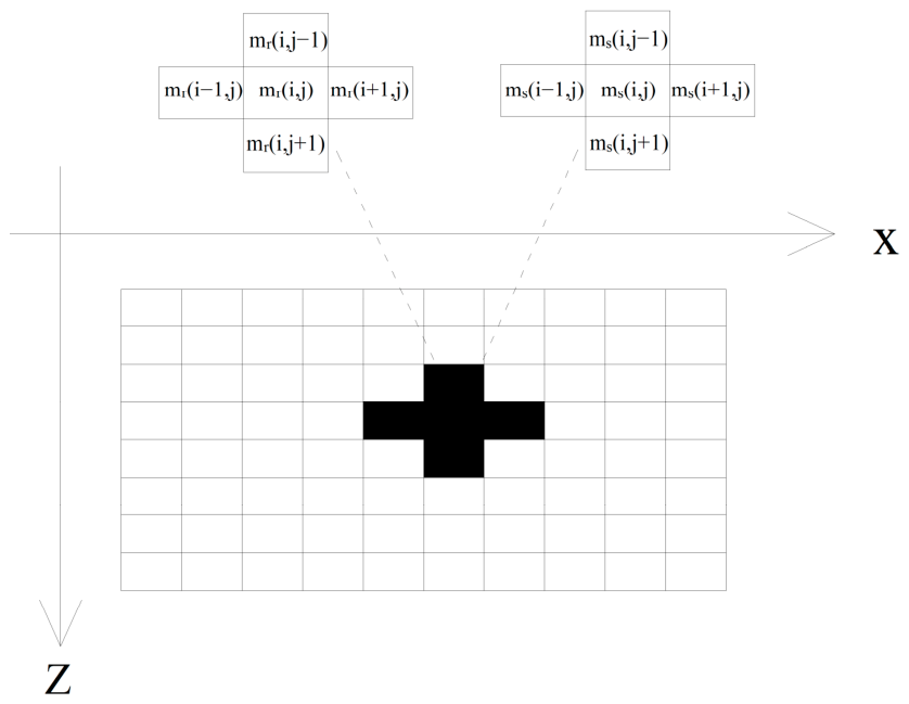
As shown in Figure 1, let $\mathrm{i}$ and $\mathrm{j}$ denote the horizontal and vertical grid indices, respectively, and let the horizontal and vertical cell sizes be $\Delta \mathrm{x}$ and $\Delta \mathsf{\epsilon }$. We discretize the cross-gradient function using the central difference quotient:

$$\begin{array}{cc}{\mathrm{t}}_{\mathrm{i},\mathrm{j}}=& {\displaystyle \frac{{\mathrm{m}}_{\mathrm{r}}(\mathrm{i},\mathrm{j}+1)-{\mathrm{m}}_{\mathrm{r}}(\mathrm{i},\mathrm{j}-1)}{{\Delta \mathrm{z}}_{\mathrm{j}}{+(\Delta \mathrm{z}}_{\mathrm{j}+1}{+\Delta \mathrm{z}}_{\mathrm{j}-1})/2}}\cdot {\displaystyle \frac{{\mathrm{m}}_{\mathrm{s}}(\mathrm{i}+1,\mathrm{j})-{\mathrm{m}}_{\mathrm{s}}(\mathrm{i}-1,\mathrm{j})}{{\Delta \mathrm{x}}_{\mathrm{i}}{+(\Delta \mathrm{x}}_{\mathrm{i}+1}{+\Delta \mathrm{x}}_{\mathrm{i}-1})/2}}-\\ & {\displaystyle \frac{{\mathrm{m}}_{\mathsf{\gamma }}(\mathrm{i}+1,\mathrm{j})-{\mathrm{m}}_{\mathsf{\gamma }}(\mathrm{i}-1,\mathrm{j})}{{\Delta \mathrm{x}}_{\mathrm{i}}{+(\Delta \mathrm{x}}_{\mathrm{i}+1}{+\Delta \mathrm{x}}_{\mathrm{i}-1})/2}}\cdot {\displaystyle \frac{{\mathrm{m}}_{\mathrm{s}}(\mathrm{i},\mathrm{j}+1)-{\mathrm{m}}_{\mathrm{s}}(\mathrm{i},\mathrm{j}-1)}{{\Delta \mathrm{z}}_{\mathrm{j}}{+(\Delta \mathrm{z}}_{\mathrm{j}+1}{+\Delta \mathrm{z}}_{\mathrm{j}-1})/2}}\end{array}$$

(4)

Figure 1. Cross-gradient grid.

The physical significance of the cross-gradient can be further understood from its mathematical expression: when resistivity and seismic impedance share the same boundaries, the cross-gradient condition ${\mathrm{t}}_{\mathrm{i},\mathrm{j}}=0$ is satisfied regardless of whether their spatial variation directions are identical or opposite. A special case may also arise: if the gradient of one physical property is zero, the cross-gradient condition ${\mathrm{t}}_{\mathrm{i},\mathrm{j}}=0$ holds irrespective of the gradient value of the other property. In all other scenarios, the condition ${\mathrm{t}}_{\mathrm{i},\mathrm{j}}\ne 0$ is likewise met. Consequently, when the two physical properties possess coincident boundaries, the cross-gradient serves to constrain the inversion of both properties.

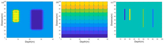
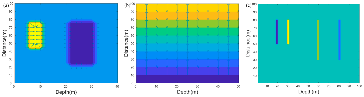
We conducted a 2-D model test to illustrate the cross-gradient function’s properties. Figure 2 shows the results. Panels (a) and (b) display cross-sections of two different physical property models. In panel (a), the model contains two anomalous bodies: a high anomaly on the left and a low anomaly on the right. In panel (b), the parameter values decrease progressively from top to bottom. Panel (c) shows the cross-gradient values between the two models. Notably, the cross-gradient values are non-zero only at the vertical boundaries of the anomalous bodies in model (a); elsewhere, they remain zero.

Figure 2. Calculation of cross-gradient values for two kinds of physical properties: (a) schematic diagram of physical property parameter model one, (b) schematic diagram of physical property parameter model two, (c) cross-gradient values.

From this model test, we observe the following characteristics of the cross-gradient function:

(1)

When one physical property parameter remains unchanged, the cross-gradient value stays zero regardless of variations in the other model.

(2)

When the parameter variation directions in both models are identical or opposite, the cross-gradient value is zero at every point.

(3)

When the variation directions are not parallel, the cross-gradient value is not uniformly zero.

(4)

The closer the structural variations in the two models, the smaller the cross-gradient value; conversely, greater structural divergence yields larger cross-gradient values.

From the perspective of solving ill-posed inverse problems, the cross-gradient constraint serves as a structural regularization that stabilizes the inversion and reduces solution non-uniqueness. By enforcing structural consistency between different physical properties, it effectively couples two otherwise independent inversions and restricts the solution space to geologically plausible models. The cross-gradient equals zero only where the two models share consistent boundary orientations or where one model is homogeneous. This property ensures that the constraint is selectively active only where common structure exists, without imposing spurious information elsewhere, which justifies its use as a physically meaningful regularization for ill-posed joint inversion.

2.2. Joint Inversion Objective Function

The geophysical joint inversion objective function comprises a data misfit term and a model smoothness term, and it is constrained subject to the condition that the cross-gradient between resistivity and wave impedance equals zero:

$$\phi =\sum (d-f\left(m_{\mathrm{r}}\right))\cdot C^{-1}\cdot \left(d-f\left(m_{\mathrm{r}}\right)\right)$$

(5)

constraint condition: $\tau \left(m_r,m_s\right)=0$

where $\mathrm{d}$ represents the observed DC resistivity data and $\mathrm{f}\left({\mathrm{m}}_{\mathrm{r}}\right)$ denotes the forward response of the physical model. Since this paper imposes constraints solely on resistivity inversion under cross-gradient conditions, for convenience, the symbol $\mathrm{m}$ will uniformly replace ${\mathrm{m}}_{\mathrm{r}}$ throughout the following discussion. The expression can thus be written concisely as:

$$\phi ={(\mathrm{d}-f\left(m\right))}^T\cdot C^{-1}\cdot \left(\mathrm{d}-f\left(m\right)\right)$$

(6)

constraint condition: $\tau \left(m\right)=0$

We solve this constrained problem using the Lagrange multiplier method. Expanding both the forward response $\mathrm{f}\left({\mathrm{m}}_{\mathrm{r}}\right)$ and the cross-gradient function $\mathsf{\tau }\left({\mathrm{m}}_{\mathrm{r}},{\mathrm{m}}_{\mathrm{s}}\right)$ in Taylor series yields:

$$f\left(m\right)=f\left(m_0+\Delta m\right)\approx f\left(m_0\right)+J\cdot \left(m-m_0\right)$$

(7)

$$\tau \left(m\right)=\tau \left(m_0+\Delta m\right)\approx \tau \left(m_0\right)+B\cdot \left(m-m_0\right)$$

(8)

where $\mathrm{B}$ is the matrix of partial derivatives of the discretized cross-gradient $\mathrm{t}$ with respect to resistivity $\mathsf{\rho }$, with elements given by

$$\begin{array}{l}{\displaystyle \frac{\partial t_{i,j}}{\partial {\rho }_{i,j+1}}}={\displaystyle \frac{1}{\Delta z_j+\left(\Delta z_{j+1}+\Delta z_{j-1}\right)/2}}\cdot {\displaystyle \frac{m_s\left(i+1,j\right)-m_s\left(i-1,j\right)}{\Delta x_i+\left(\Delta x_{i+1}+\Delta x_{i-1}\right)/2}}\\ {\displaystyle \frac{\partial t_{i,j}}{\partial {\rho }_{i,j-1}}}={\displaystyle \frac{-1}{\Delta z_j+\left(\Delta z_{j+1}+\Delta z_{j-1}\right)/2}}\cdot {\displaystyle \frac{m_s\left(i+1,j\right)-m_s\left(i-1,j\right)}{\Delta x_i+\left(\Delta x_{i+1}+\Delta x_{i-1}\right)/2}}\\ {\displaystyle \frac{\partial t_{i,j}}{\partial {\rho }_{i+1,j}}}={\displaystyle \frac{1}{\Delta x_i+\left(\Delta x_{i+1}+\Delta x_{i-1}\right)/2}}\cdot {\displaystyle \frac{m_s\left(i,j+1\right)-m_s\left(i,j-1\right)}{\Delta z_j+\left(\Delta z_{j+1}+\Delta z_{j-1}\right)/2}}\\ {\displaystyle \frac{\partial t_{i,j}}{\partial {\rho }_{i-1,j}}}={\displaystyle \frac{-1}{\Delta x_i+\left(\Delta x_{i+1}+\Delta x_{i-1}\right)/2}}\cdot {\displaystyle \frac{m_s\left(i,j+1\right)-m_s\left(i,j-1\right)}{\Delta z_j+\left(\Delta z_{j+1}+\Delta z_{j-1}\right)/2}}\end{array}$$

(9)

In Equation (9), the indices i and j refer to the vertical and horizontal grid directions, respectively. The horizontal grid step is typically one-half or one-quarter of the electrode spacing, whereas the vertical grid is non-uniform and can be flexibly designed.

Incorporating the constraint into the objective function via Lagrange multipliers gives:

$$\mathsf{\Psi }=(d-f){)}^T\cdot C^{-1}\cdot \left(d-f(m)\right)+\mathsf{\Lambda }\cdot \tau \left(m\right)$$

(10)

Substituting Equations (7) and (8) yields:

$$\mathsf{\Psi }={(d-f\left(m_0\right)-J\cdot \left(m\cdot m_0\right))}^T\cdot C^{-1}\cdot \left(d-f\left(m_0\right)-J\cdot \left(m\cdot m_0\right)\right)+\mathsf{\Lambda }\cdot \left(\tau \left(m_0\right)+B\cdot \left(m\cdot m_0\right)\right)$$

(11)

Among them, $\mathsf{\Lambda }$ refers to the Lagrange operator.

When $\hat{\mathrm{d}}=\mathrm{d}-\mathrm{f}\left({\mathrm{m}}_0\right),\hat{\mathsf{\tau }}=\mathsf{\tau }\left({\mathrm{m}}_0\right)$, the above equation can be transformed as:

$$\mathsf{\Psi }={(\hat{d}-J\cdot \Delta m)}^T\cdot C^{-1}\cdot \left(\hat{d}-J\cdot \Delta m\right)+\mathsf{\Lambda }\cdot \left(\hat{\tau }+B\cdot \Delta m\right)$$

(12)

The model update $\Delta \mathrm{m}$ is then obtained by seeking the extremum of the cross-gradient-constrained objective function.

In practice, we solve this problem using the fmincon toolbox in MATLAB R2020b, specifically employing the active-set method. This algorithm uses the conjugate gradient method to explore a face of the feasible region, obtains an estimate of the active set, and then departs from that face along the negative gradient to refine the estimate. To accelerate convergence and avoid local extrema, we initialize the inversion with the result from an unconstrained resistivity inversion.

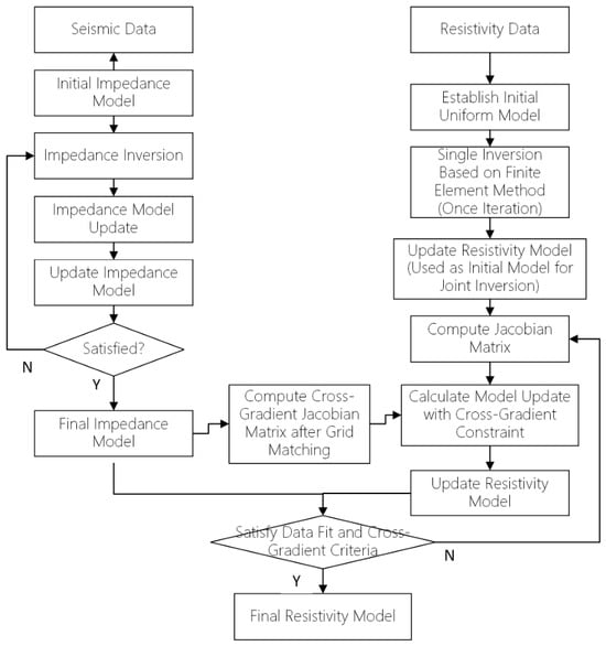
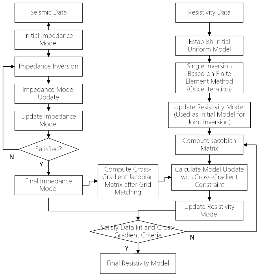
2.3. Joint Inversion Workflow

Directly incorporating the cross-gradient function into the joint inversion may interfere with the objective function in least-squares smooth inversion. This interference can hinder proper data fitting, increase computational demands, or even prevent convergence.

To address these issues, we adopt a more robust workflow: first, we perform wave impedance inversion on the seismic data alone. The resulting wave impedance model then serves as the initial model for the joint inversion of both data types, thereby accelerating iteration. Figure 3 presents a concise flowchart of the joint inversion procedure.

Figure 3. Joint Inversion Chart.

3. Results

We developed a joint inversion program in MATLAB based on the theory described above. This program jointly inverts wave impedance and resistivity data. We developed a joint inversion program in MATLAB based on the theory described above. Regarding the numerical implementation, all inversions were performed using the MATLAB fmincon toolbox with the active-set algorithm. The maximum number of iterations was uniformly set to 80 for all test cases to thoroughly verify the convergence stability of the algorithm (in practice, stable convergence is typically achieved within approximately 15 iterations for both separate and joint inversions). Since this study primarily focuses on methodological validation, iteration termination was based on reaching the maximum iteration count, although a convergence criterion based on the relative change in the objective function was already implemented in our code. The initial model for joint inversion was provided by the result of separate resistivity inversion, which helped accelerate convergence and avoid local minima. This program jointly inverts wave impedance and resistivity data. We compare the joint inversion results with those from separate inversion to validate the feasibility and stability of the algorithm. We compare the joint inversion results with those from separate inversion to validate the feasibility and stability of the algorithm. In the synthetic model design, the top burial depth of all anomalies is fixed at 20 m. This choice isolates the effect of cross-gradient constraints on lateral resolution, as our focus is on distinguishing anomalies at different horizontal separations rather than on depth effects.

3.1. Analysis of Joint Inversion Algorithm Effectiveness

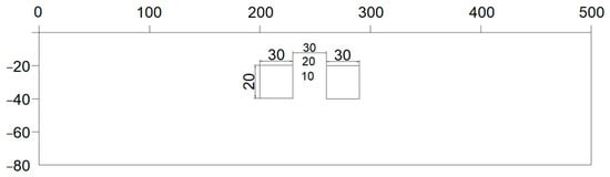
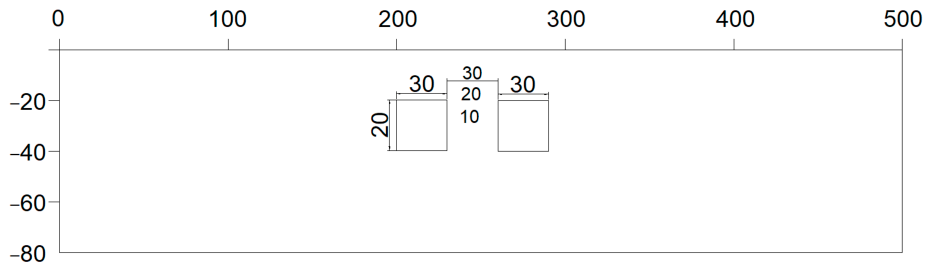
Figure 4 depicts the synthetic model: two rectangular prisms embedded in a homogeneous half-space. Each prism measures 30 m in length, 20 m in width, and has a top burial depth of 20 m. The background half-space has a resistivity of 100 $\mathsf{\Omega }\cdot \mathrm{m}$, a P-wave velocity of 2000 m/s, and a density of 2 g/cm³. The anomalous bodies have a resistivity of 1000 $\mathsf{\Omega }\cdot \mathrm{m}$, a P-wave velocity of 2500 m/s, and a density of 2.2 g/cm³. Panels (a), (b), and (c) show the model with inter-body separations of 30 m, 20 m, and 10 m, respectively. The morphology and boundary locations of resistivity, velocity, and density are identical, and the property variation directions at boundaries are also the same.

Figure 4. Schematic diagram of two high-resistance and high-speed anomaly bodies models (each prism is 30 m in length and 20 m in width, with a top burial depth of 20 m. The background resistivity is 100 Ω·m; the anomalies have resistivity of 1000 Ω·m).

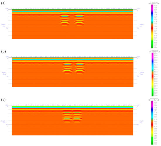
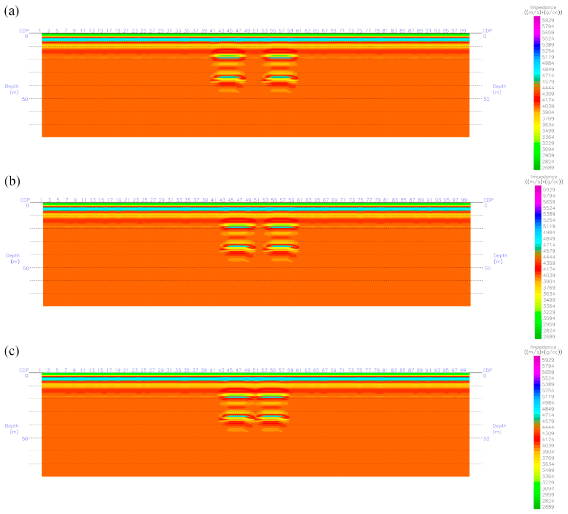
Figure 5 shows the wave impedance inversion results obtained using Strata V2.0 for the three separation distances. The upper and lower interfaces of the anomalous bodies appear clearly in all panels. However, the region between the bodies is poorly resolved. At separations of 30 m and 20 m, the two bodies are clearly distinguishable. At 10 m separation, although the bodies can still be discerned, their upper interfaces appear connected, and the true separation distance becomes difficult to determine accurately.

Figure 5. The results of wave impedance inversion of two high-resistance and high-speed anomaly bodies models: (a) separation 30 m, (b) separation 20 m, (c) separation 10 m.

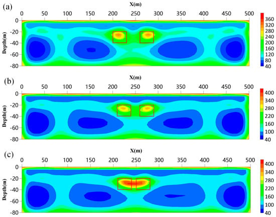
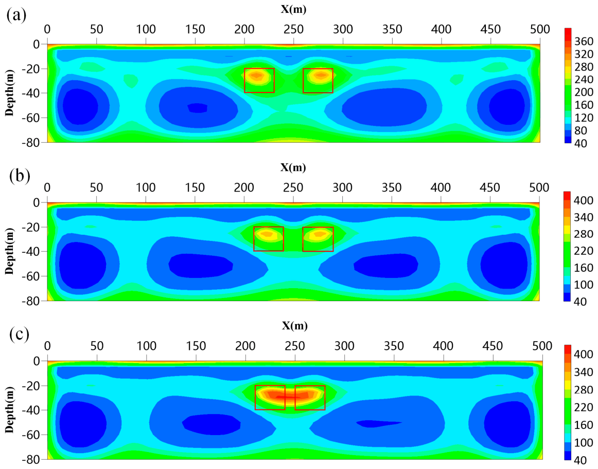
Figure 6 presents the separate inversion results obtained via least-squares inversion of the forward responses using MATLAB. The resistivity sounding survey employs a Wenner array with an electrode separation of 10 m; red outlines mark the true positions of the anomalous bodies. At separations of 30 m and 20 m (panels a and b), the two bodies can be distinguished, but their inverted positions deviate noticeably from the true locations, and their shapes and sizes remain poorly defined. At 10 m separation (panel c), the separate inversion can no longer resolve the two bodies as distinct entities. Moreover, as the separation decreases, the maximum resistivity at the center of the anomalous zone drops continuously from 880 $\mathsf{\Omega }\cdot \mathrm{m}$ to 400 $\mathsf{\Omega }\cdot \mathrm{m}$, deviating severely from the true value. The inversion thus fails to provide an accurate interpretation.

Figure 6. Separate inversion results of resistivity data of two high-resistance and high-speed anomaly bodies models: (a) separation 30 m, (b) separation 20 m, (c) separation 10 m. The red boxes indicate the locations of the anomaly bodies.

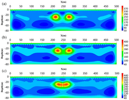
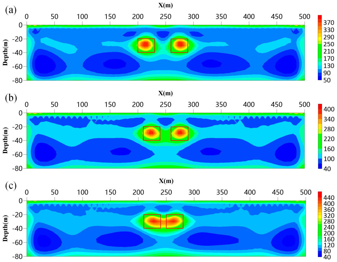
Figure 7 shows the corresponding joint inversion results constrained by seismic data. In contrast to the separate inversion results, the joint inversion clearly distinguishes the two anomalous bodies at all three separations, including 10 m. The center positions and boundary extents of the anomalous zones in panels (a), (b), and (c) all lie close to the true positions. A narrow high-resistivity zone appears between the two bodies in panel (c), but this has minimal impact on interpretation. As the separation decreases, the maximum resistivity value at the anomalous zone center declines from 880 $\mathsf{\Omega }\cdot \mathrm{m}$ to 440 $\mathsf{\Omega }\cdot \mathrm{m}$, and the error relative to the true resistivity increases.

Figure 7. Combined inversion result of two high-resistance and high-speed anomaly bodies models: (a) separation 30 m, (b) separation 20 m, (c) separation 10 m. The red boxes indicate the locations of the anomaly bodies.

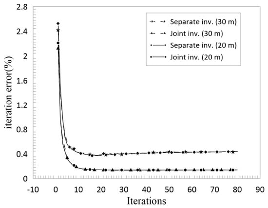
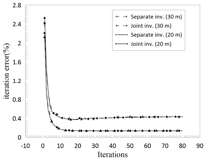
Figure 8 shows a comparison of iterative inversion speeds between the resistivity-only inversion and the joint inversion constrained by seismic data, for cases where the horizontal separation between the two high-resistivity anomalous bodies is 30 m, 20 m, and 10 m, respectively. The inversion errors reported and expressed as percentages, are defined as the ratio of the data misfit norm to the norm of the observed data, which serves as a quantitative quality metric for evaluating the solution accuracy of the inverse problem. In separate inversion, the first-iteration error increases as the separation decreases, with values of 2.415%, 2.527%, and 2.751%. After ten iterations, the errors become comparable but exhibit occasional fluctuations. Notably, as iterations continue, the error begins to increase rather than stabilize. For the joint inversion, the first-iteration error also increases with decreasing separation (2.12%, 2.208%, and 2.387%), but the values are consistently lower than those of separate inversion. After ten iterations, the error stabilizes at approximately 0.138%—far smaller than the separate-inversion errors—and shows no divergence with further iterations.

Figure 8. Convergence curves of inversion error versus iteration number for separate and joint inversion in inversion of two high-resistance and high-speed anomaly bodies models.

3.2. Stability Analysis of the Joint Inversion Algorithm

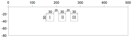
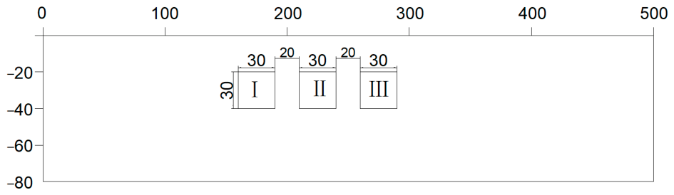
Figure 9 illustrates a model with three rectangular prisms in a homogeneous half-space. Each prism measures 30 m × 30 m in plan view and has a top burial depth of 20 m. The horizontal separation between adjacent prisms is 20 m. The background medium has a resistivity of 100 $\mathsf{\Omega }\cdot \mathrm{m}$, a P-wave velocity of 2000 m/s, and a density of 2 g/cm³. Anomalous Body I has a resistivity of 1000 $\mathsf{\Omega }\cdot \mathrm{m}$, a P-wave velocity of 2000 m/s, and a density of 2 g/cm³. Anomalous Body II has identical properties. Anomalous Body III has a resistivity of 1000 $\mathsf{\Omega }\cdot \mathrm{m}$, a P-wave velocity of 2500 m/s, and a density of 2.5 g/cm³. Again, the morphology and boundary locations of all three properties are identical, as are the variation directions at the boundaries.

Figure 9. Schematic diagram of three different anomaly bodies models.

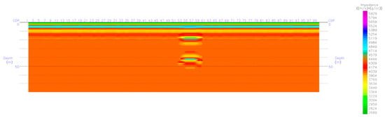
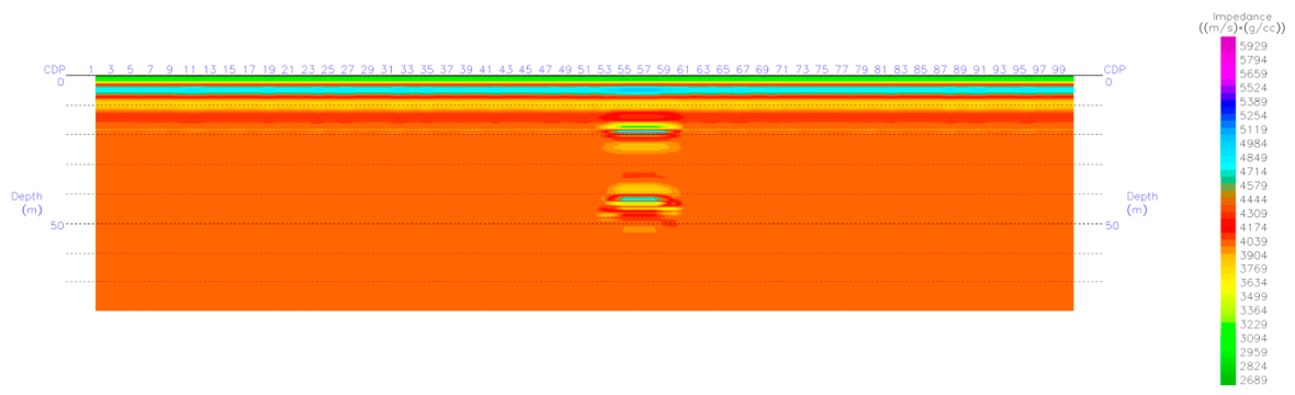
Figure 10 shows the wave impedance inversion results after processing with Strata. To simulate realistic field conditions, we provided well log data only within the homogeneous background, not at the anomalous body locations. Consequently, only two seismic events appear—corresponding to the upper and lower interfaces of Anomalous Body III. The bodies with resistivity contrasts but no velocity contrast relative to the background (Anomalous Bodies I and II) produce no response.

Figure 10. The results of wave impedance inversion of three different anomaly bodies models.

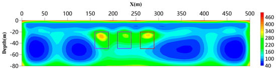
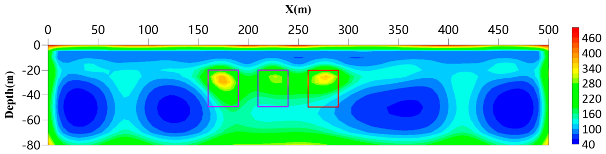
Figure 11 displays the separate inversion results obtained using the least-squares method. The true positions of the three anomalous bodies are outlined. Two relatively distinct high-resistivity zones are visible, but the intermediate zone remains poorly resolved, likely due to the larger separation between Anomalous Bodies I and III. Overall, the separate inversion fails to clearly delineate the three bodies. The inverted center positions for Anomalous Bodies I and III are slightly shifted upward, and the shapes and sizes remain uncertain.

Figure 11. Separate inversion results of resistivity data of three different anomaly bodies models. The red boxes indicate the locations of the anomaly bodies.

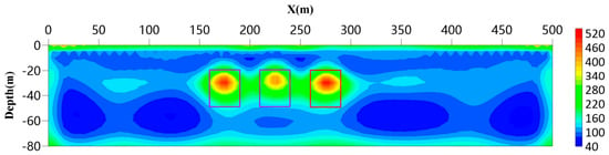
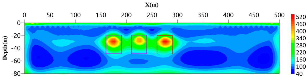
Figure 12 shows the joint inversion results constrained by seismic data. In contrast to the separate inversion, the joint inversion reveals three distinct high-resistivity zones. The center positions and boundary extents of these zones closely match the true positions of the three anomalous bodies. Thus, even though Anomalous Bodies I and II are absent from the seismic model, the seismic-constrained joint inversion outperforms the separate inversion.

Figure 12. Combined inversion result of three different anomaly bodies models. The red boxes indicate the locations of the anomaly bodies.

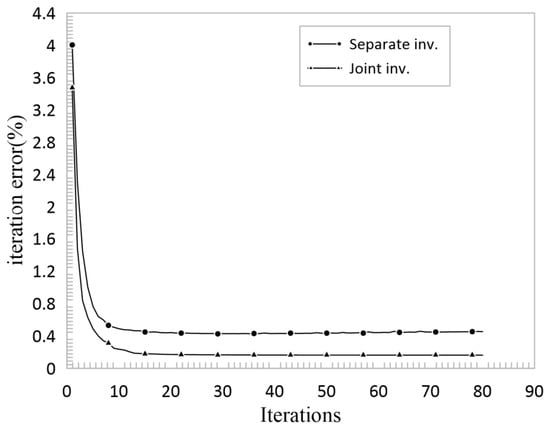
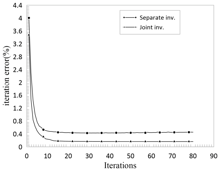
Figure 13 compares convergence rates for the separate and joint inversion when the anomalous body structures are inconsistent. The separate inversion starts with a first-iteration error of 4.004% and converges after approximately 12 iterations, stabilizing at an error of 0.432%. The joint inversion begins with a lower first-iteration error of 3.472%, stabilizes after 14 iterations without significant fluctuation, and reaches a final error of 0.163%. Although the joint inversion converges more slowly, it achieves a substantially smaller final error. We attribute the slower initial convergence to the fact that only Anomalous Body III appears in the seismic starting model, and the close separation of the three bodies in the resistivity model amplifies volume effects. The consistently lower error values achieved by the joint inversion across all tested models further support the effectiveness of the cross-gradient constraint in improving inversion reliability.

Figure 13. Convergence curves of inversion error versus iteration number for separate and joint inversion in inversion of three different anomaly bodies models.

4. Discussion

This study investigated the wave impedance inversion of seismic data and the smoothness-constrained least-squares inversion of resistivity data. We employed the cross-gradient function to characterize the structural relationship between the two physical property parameters and to incorporate seismic wave impedance data into the resistivity inversion process, thereby achieving joint inversion. The algorithm was implemented in MATLAB and tested on multiple synthetic models.

The principal contributions can be discussed in relation to previous approaches. First, we discretized the cross-gradient function using central differences and derived its fundamental properties: the cross-gradient equals zero only when the structural variations in the two physical property parameters are consistent, or when one of the models is homogeneous. This property makes the cross-gradient a more flexible structural constraint compared to explicit petrophysical coupling (e.g., Archie’s law), because it does not require a predefined resistivity–velocity relationship and can accommodate scenarios where such a relationship is absent or unknown.

The structurally constrained joint inversion was implemented by incorporating the cross-gradient term into the objective function and solving it via the Lagrange multiplier method. This framework relies solely on structural similarity, which avoids potential biases introduced by inaccurate petrophysical models and broadens the applicability to various geological settings. Compared with the decoupled strategy proposed by Gao et al. [19,20], our approach focuses on a direct incorporation of the constraint, providing an alternative for smaller-scale near-surface problems.

This study only tested synthetic models with simple geometries. The performance under field conditions, where noise levels and model complexities are higher, remains to be evaluated. However, Although we have not yet conducted systematic tests with noisy data, it is worth noting that the cross-gradient constraint primarily relies on structural consistency between the two physical properties rather than on absolute value matching. As such, this constraint inherently provides a degree of suppression against random noise, and the method is expected to effectively delineate major boundaries under moderate noise levels. It is also worth noting that when the two properties lack structural correlation in certain regions, the cross-gradient constraint automatically becomes inactive and the joint inversion reverts to separate inversion. Thus, the method does not produce worse results than separate inversion, but offers no additional improvement in such regions. It is therefore best suited for settings where resistivity and wave impedance share common structural features, and is not intended for cases where their boundaries are entirely different.

Future work will focus on three main directions: (1) validation with field data from engineering and hydrogeological surveys, (2) extension of the algorithm to three-dimensional cases, and (3) integration with other geophysical methods such as the transient electromagnetic (TEM) method.

5. Conclusions

The synthetic tests demonstrate that compared with separate inversion, the cross-gradient-based joint inversion delineates anomalous body boundaries more accurately and sharply. The inverted boundaries lie closer to the true model, the resolution of multiple anomalous bodies improves substantially, and the recovered physical property values more closely approach the actual values. The convergence rate and stability also improve.

Importantly, the cross-gradient-constrained joint inversion algorithm imposes strong constraints only where the structural variations in the two properties are consistent. It does not adversely affect regions of inconsistent variation and is not prone to introducing external errors, which ensures the robustness of the method.

In summary, this work confirms that the joint inversion of wave impedance and resistivity data constrained by the cross-gradient function is effective and reliable. It significantly reduces the non-uniqueness inherent in geophysical inversion and yields more accurate and stable inversion results, showing promising potential for near-surface engineering and hydrogeological investigations.

References

- Jackson, D.D. Interpretation of inaccurate, insufficient and inconsistent data. Geophys. J. Int. 1972, 28, 97–109. [Google Scholar] [CrossRef] [Scilit]
- Liu, G. Review and prospect—Solid earth geophysics in the 21st century. Prog. Geophys. 2002, 17, 191. (In Chinese) [Google Scholar] [CrossRef]
- Liu, Y.; Lu, Q.; Meng, G.; Yan, J.; Zhang, K.; Yang, Z. Research status and prospect of magnetotelluric and seismic joint inversion. Prog. Geophys. 2012, 27, 2444–2451. (In Chinese). Available online: http://en.dzkx.org/article/doi/10.6038/j.issn.1004-2903.2012.06.019 (accessed on 23 April 2026).
- Vozoff, K.; Jupp, D.L.B. Joint inversion of geophysical data. Geophys. J. Int. 1975, 42, 977–991. [Google Scholar] [CrossRef] [Scilit]
- Raiche, A.P.; Jupp, D.L.B.; Rutter, H.; Vozoff, K. The joint use of coincident loop transient electromagnetic and Schlumberger sound to resolve layered structures. Geophysics 1985, 50, 1618–1627. [Google Scholar] [CrossRef] [Scilit]
- Sasaki, Y. Two-dimensional joint inversion of magnetotelluric and dipole-dipole resistivity data. Geophysics 1989, 54, 254–262. [Google Scholar] [CrossRef] [Scilit]
- Hu, J. Joint inversion of transient electromagnetic sounding and direct current sounding data. Oil Geophys. Prospect. 1989, 24, 549–558. (In Chinese) [Google Scholar]
- Dobróka, M.; Gyulai, Á.; Ormos, T.; Csókás, J.; Dresen, L. Joint inversion of seismic and geoelectric data recorded in an underground coal mine. Geophys. Prospect. 1991, 39, 643–665. [Google Scholar] [CrossRef] [Scilit]
- Jing, R.; Bao, G.; Lin, J.; Chen, S. A joint inversion method for geophysical data based on data fusion: A case study of VES and MT. Chin. J. Geophys. 2004, 47, 143–150. (In Chinese) [Google Scholar] [CrossRef]
- Meju, M.A.; Gallardo, L.A.; Mohamed, A.K. Evidence for correlation of electrical resistivity and seismic velocity in heterogeneous near-surface materials. Geophys. Res. Lett. 2003, 30, 1373. [Google Scholar] [CrossRef] [Scilit]
- Gallardo, L.A.; Meju, M.A. Characterization of heterogeneous near-surface materials by joint 2D inversion of dc resistivity and seismic data. Geophys. Res. Lett. 2003, 30, 1658. [Google Scholar] [CrossRef] [Scilit]
- Gallardo, L.A.; Meju, M.A. Joint two-dimensional DC resistivity and seismic travel time inversion with cross-gradients constraints. J. Geophys. Res. Solid Earth 2004, 109, B03311. [Google Scholar] [CrossRef] [Scilit]
- Gallardo, L.A.; Meju, M.A. Joint two-dimensional cross-gradient imaging of magnetotelluric and seismic traveltime data for structural and lithological classification. Geophys. J. Int. 2007, 169, 1261–1272. [Google Scholar] [CrossRef] [Scilit]
- Yang, Y.; He, Z.; Wang, X.; Luo, W. Simulation analysis of AMT, TEM, and VES stratigraphic response characteristics and discussion on joint inversion. Prog. Geophys. 2008, 23, 1550–1555. (In Chinese). Available online: https://lzlib.cgl.org.cn/auto/db/detail.aspx?agfi=0&cid=0&cls=0&count=10&db=100053&md=510&mdd=510&msd=510&pd=4&pdd=4&prec=False&psd=4&rid=306576&showgp=False&uni=True%5D (accessed on 23 April 2026).
- Chen, X.; Yu, P.; Zhang, L.; Li, Y.; Wang, J. Regularized simultaneous joint inversion of magnetotelluric and seismic data. Seismol. Geol. 2010, 32, 402–408. (In Chinese) [Google Scholar] [CrossRef]
- Moorkamp, M.; Heincke, B.; Jegen, M.; Roberts, A.W.; Hobbs, R.W. A framework for 3-D joint inversion of MT, gravity and seismic refraction data. Geophys. J. Int. 2011, 184, 477–493. [Google Scholar] [CrossRef] [Scilit]
- Peng, M.; Tan, H.; Jiang, M.; Qian, H.; Tan, J. Three-dimensional joint inversion of magnetotelluric and seismic traveltime data based on cross-gradient coupling. Chin. J. Geophys. 2013, 56, 2728–2738. (In Chinese) [Google Scholar] [CrossRef]
- Bennington, N.L.; Zhang, H.; Thurber, C.H.; Bedrosian, P.A.; Zoback, M.D. Joint inversion of seismic and magnetotelluric data in the Parkfield region of California using the normalized cross-gradient constraint. Pure Appl. Geophys. 2015, 172, 1033–1052. [Google Scholar] [CrossRef] [Scilit]
- Gao, J.; Zhang, H. Two-dimensional joint inversion of seismic traveltime and full-channel direct-current resistivity with cross-gradient alternating structure constraints. Chin. J. Geophys. 2016, 59, 4310–4322. (In Chinese). Available online: https://kns.cnki.net/kcms2/article/abstract?v=4K0tw7BxpDF-OJhsZdAn6UAwYUoL0j7j_TjyoTsJ2ucqgPp_vsYjsM8SeY-rwm_Rv-_DwaRr8Dj7ikiifpouVtlfYlCppkwv67kqYk26HXfOr0-RunjW2rWFxOcekYs9SpFpg9-KV8PlSXzSaszwHX9UKPIiGKELuUqf4EjJ3EGpDiV1eOV6yw==&uniplatform=NZKPT&language=CHS (accessed on 23 April 2026).
- Gao, J.; Zhang, H.; Fang, H.; Li, N. An efficient 3-D joint inversion strategy for seismic traveltime and direct-current resistivity with cross-gradient structure constraints. Chin. J. Geophys. 2017, 60, 3628–3641. (In Chinese) [Google Scholar]
- Colombo, D.; McNeice, G.; Rovetta, D.; Sandoval-Curiel, E.; Turkoglu, E.; Sena, A. High-resolution velocity modeling by seismic-airborne TEM joint inversion: A new perspective for near-surface characterization. Lead Edge 2016, 35, 977–985. [Google Scholar] [CrossRef] [Scilit]
- Shi, Z.; Hobbs, R.W.; Moorkamp, M.; Tian, G.; Jiang, L. 3-D cross-gradient joint inversion of seismic refraction and DC resistivity data. J. Appl. Geophys. 2017, 141, 54–67. [Google Scholar] [CrossRef] [Scilit]
- Pak, Y.-C.; Li, T.; Kim, G.-S. 2D data-space cross-gradient joint inversion of MT, gravity and magnetic data. J. Appl. Geophys. 2017, 143, 212–222. [Google Scholar] [CrossRef] [Scilit]
- Zhang, R. Research and Application of 2-D Cross-Gradient Joint Inversion of Gravity, Magnetic, Electrical and Seismic Data. Master’s Thesis, Jilin University, Changchun, China, 2017. [Google Scholar]
- Yin, C.; Sun, S.; Gao, X.; Liu, Y.; Chen, H. Three-dimensional joint inversion of magnetotelluric and gravity data based on local correlation constraints. Chin. J. Geophys. 2018, 61, 358–367. (In Chinese) [Google Scholar] [CrossRef]
- Li, F.; Cheng, J.; Yang, S.; Wen, L.; Dong, Y. Experimental study on joint inversion of water conducted karstic collapse column based on mine TEM and seismic exploration. J. China Coal Soc. 2020, 45, 2472–2481. (In Chinese) [Google Scholar] [CrossRef]
- Yan, Z.; Tan, H.; Peng, M.; Kong, W.; Wu, P. Three-dimensional joint inversion of gravity, magnetic and magnetotelluric data based on cross-gradient constraints. Chin. J. Geophys. 2020, 63, 736–752. (In Chinese) [Google Scholar]
- Zhang, Z.; Liao, X.; Cao, Y.; Hou, Z.; Fan, X.; Xu, Z.; Shi, Z. Joint inversion of gravity anomaly and gravity gradient anomaly based on deep learning. Chin. J. Geophys. 2021, 64, 1435–1452. (In Chinese) [Google Scholar] [CrossRef]
- He, H.; Li, T.; Zhang, R.; Zhu, W. Three-dimensional joint inversion of gravity, gravity gradient and magnetotelluric data with smooth focusing structure constraints. Chin. J. Geophys. 2022, 65, 1822–1838. (In Chinese) [Google Scholar] [CrossRef]
- Liu, J.; Zhang, Z.; Zhou, F.; Li, M.; Ou, Y.; Yang, L.; Yi, K. Two-dimensional joint inversion of DC resistivity and seismic traveltime tomography with FCM clustering constraints. Chin. J. Geophys. 2023, 66, 3048–3059. (In Chinese) [Google Scholar] [CrossRef]
- Wang, L.; Liu, W.; Xi, Z.; Xue, J.; Hou, H.; Long, X.; Xue, W. Deep learning joint inversion of audio magnetotelluric and transient electromagnetic data. Chin. J. Geophys. 2024, 67, 4372–4384. (In Chinese). Available online: http://en.dzkx.org/article/doi/10.6038/cjg2023R0582 (accessed on 23 April 2026).
- Kong, F.; Tan, H.; Liu, J. Research on 2-D joint inversion of marine controlled-source electromagnetic and seismic full waveform. Geophys. Geochem. Explor. 2024, 48, 67–76. (In Chinese). Available online: https://kns.cnki.net/kcms2/article/abstract?v=4K0tw7BxpDGDxT2xG3FOst2gEBsKm4KoSSYCqDF87f8Aokwxo3qYlM_8A6VLd66FQSh7vGayU4tAwwo6x-1x5Mor7CvB2S4aAz71Xp-tfNrhHqgNAENY29bYrF3WJ2a9XOg8TuPd4BeSAFHKkHieyYUVaAp-SuSlUJmgFFhkulNBts6KWB-4vQ==&uniplatform=NZKPT&language=CHS (accessed on 23 April 2026).
- Zhang, C.; Li, J.; Cao, H. Integrating elastic neural network seismic waveform with petrophysical inversion framework for critical zone properties estimation. IEEE Trans. Geosci. Remote Sens. 2024, 62, 4510713. [Google Scholar] [CrossRef] [Scilit]
- Penta de Peppo, G.; Cercato, M.; De Donno, G. Cross-gradient joint inversion and clustering of ERT and SRT data on structured meshes incorporating topography. Geophys. J. Int. 2024, 239, 1155–1169. [Google Scholar] [CrossRef] [Scilit]
Disclaimer/Publisher’s Note: The statements, opinions and data contained in all publications are solely those of the individual author(s) and contributor(s) and not of MDPI and/or the editor(s). MDPI and/or the editor(s) disclaim responsibility for any injury to people or property resulting from any ideas, methods, instructions or products referred to in the content. |
© 2026 by the authors. Licensee MDPI, Basel, Switzerland. This article is an open access article distributed under the terms and conditions of the Creative Commons Attribution (CC BY) license.