Pre-Seismic Ground Dislocations from Interferometric Satellite Synthetic Aperture Radar Images as Predictors of Earthquake Magnitude and Epicenter Localization

Abstract

This work aims to determine whether pre-seismic ground dislocations extracted from interferometric satellite synthetic aperture radar (InSAR) imagery contain predictive information for distinguishing between two magnitude classes of an upcoming earthquake, assuming that an earthquake’s occurrence is already imminent. For this reason, twenty-three earthquakes of various magnitudes that occurred in Greece during the year 2020 were analyzed using SAR data to construct a time-series of five six-day InSAR images for each earthquake, spanning a total 24-day period before the earthquake. For each earthquake, four ground dislocation images covering the area around each earthquake were derived from the interferograms, each showing the dislocation during a six-day time interval. Images showing the total ground dislocation during the entire 24-day period before the earthquake were also produced by fusing the four images. Three machine learning classifiers were used to relate the earthquake magnitude class to pre-seismic ground dislocations. High accuracies were obtained with both support vector machine (SVM) and random forest (RF), yet they were highly dependent on the type of images used. In a subsequent analysis, five regression models were applied to estimate the earthquakes’ epicenters from dislocation images. The results reveal that the proposed approach is able to achieve well-localized epicentral area prediction, indicating the potential predictive value of this tool for seismic hazard assessment and emergency planning.

1. Introduction

Among natural hazards, earthquakes are prominent due to their sudden unpredictable onset and their potential for severe destruction directly affecting human lives and critical infrastructure. According to the World Health Organization (WHO), earthquakes are responsible for approximately 750,000 deaths globally within two decades, averaging 37,500 deaths per year [1]. Human safety could be ensured if the exact timing, magnitude and location of incoming earthquakes could be accurately predicted [2]. Despite advancements in seismology and improvements in long-term predictions [3,4] through monitoring of seismic waves and tectonic activity, short-term prediction within a couple of months or days before the earthquake remains challenging [5].

Pre-seismic ground movements are subtle ground movements that occur before an earthquake. Although detectable, such signals are not currently used for reliable earthquake prediction, since they are not consistently present before all earthquakes, and their patterns vary depending on local geology and tectonic stress. Moreover, subtle ground movements can also be caused by other effects, such as human activity, which makes it difficult to isolate true pre-seismic signals from noise [6,7,8,9,10]. The detection of such movements requires precise geodetic techniques such as interferometric synthetic aperture Radar (InSAR). This method measures ground displacement by analyzing phase differences between co-registered complex SAR acquisitions obtained at different points in times [11,12]. Recent advancements in artificial intelligence (AI) methods have motivated the exploration of whether deformation patterns extracted from InSAR time-series may contain useful information related to short-term earthquake forecasting [13,14,15,16,17].

Based on the above, this work aims to determine whether pre-seismic ground movements, detectable via InSAR, contain predictive information about the magnitude class of upcoming earthquakes. Compared to the number of published studies on coseismic and post-seismic ground movements, there are a limited number of studies concerning pre-seismic deformations. Delouis et al. [18] used InSAR and high-rate Global Positioning System (GPS) data to detect rupture along the subduction plate interface and slippage before the Mw 8.8 earthquake in Chile in 2010. Vaka et al. [19] reported ground movements using InSAR before the Mw 7.3 earthquake that struck the Iran–Iraq border region in November 2017. Similarly, InSAR and global navigation satellite system (GNSS) data were employed by Guo et al. [20] to detect fault slips, ground deformation, and elevated shear strain before the Mw 6.9 earthquake in China in January 2022. Pre-seismic ground dislocations were also detected by InSAR in the case of the 2015 Mw 7.8 earthquake in Nepal [21], the 1999 Mw 7.6 earthquake in Taiwan [22], the 2009 Mw 6.3 L’Aquila earthquake in Italy [23,24], the 2021 Mw 4.6 and 4.4 events in Vienna Basin, Austria [25], and the Mw 6.9 earthquake north of Samos Island, Greece, in October 2020 [26]. Inter-seismic deformations were also recorded by Chlieh et al. [27] in the subduction zone of North Chile, by Shokrzade et al. [28] in the 2003 Bam Earthquake in Iran, and by Wang et al. [29] for the 2022 Mw 6.7 earthquake in Menyuan, Tibet. All of these works collectively indicate the capability of InSAR to detect crystal deformation; however, they do not establish a consistent or generalizable relationship between short-term pre-seismic deformation and earthquake magnitude.

Machine learning has also been applied to deformation-related problems. An improved, high-accuracy InSAR building model, using deep learning, was proposed by Kim et al. [30]. The model could predict the magnitude of ground movements before earthquakes. However, the model only predicted the extent of ground movements, not the earthquake magnitude. To predict the timing of earthquake occurrences, Norisugi et al. [31] developed a machine learning model reporting an R² score of 0.87 for predicting the time remaining before the main shock of an earthquake. However, the model has only been tested on artificial earthquakes generated by computer simulations and not on actual earthquake datasets. Alkan et al. [32] used ground movements to calculate pre-seismic or post-seismic tectonic stress accumulation from 1912 to 2023 in the Marmara Sea region, Turkey, and to relate them to the estimated likelihood of earthquakes of specific magnitudes over extended timescales. In all of the aforementioned related published literature that connected ground dislocations to earthquake occurrence, only the territory around one single earthquake was examined, while correlation of ground dislocations to the earthquake magnitude is not reported in the literature apart from one exception; Alkan et al. [32], in their work, used actual InSAR data and developed a magnitude prediction model, which was trained with tectonic stress data for a specific area. Significant probabilities for the occurrence of earthquakes of a certain magnitude were found only for extended time periods, often over 50 years. Moreover, retraining of the algorithms would be required to apply the methodology to a different geographic area, since it focused on a relatively small geographic area, that of the sea of Marmara. The latter work remains significant as it indicates the feasibility of predicting earthquake magnitude from ground dislocations. Yet it differs significantly from our work in the aspects that it uses tectonic stress instead of direct ground dislocations and a satisfactory prediction accuracy depends on the time the earthquake is expected to occur, which is in the range of years or decades.

In contrast to these works, the present work aims to investigate whether short-term pre-seismic ground dislocations contain information that could be used to classify the magnitude class of upcoming events. Moreover, the proposed analysis considers 23 earthquakes, covering a larger geographic area, encompassing the entire Greek region and its close neighborhood. It must be highlighted that the objective of this work is not to predict whether an earthquake will occur, but rather to determine whether, considering that an earthquake is imminent, the associated pre-seismic deformation patterns can be used to classify the magnitude class of the upcoming event into two magnitude classes.

To this end, this work aims to investigate the potential of satellite-based ground deformation patterns serving as reliable complementary precursors for earthquake magnitude prediction. The proposed method aspires to bridge the gap between earthquake monitoring and short-term prediction, which has great implications for early warning systems in ensuring risk reduction and overall public safety. Specifically, in this work, two classes of earthquake magnitudes can be predicted, over or less than Mw 4.6, in any region of Greece and its close neighborhood, based purely on InSAR data. Pre-seismic ground movements occurring around the epicenter of earthquakes for a period of 24 to 28 days before the seismic event, as calculated from interferograms, are used to train machine learning models for predicting the magnitude class of an earthquake when it occurs. The contributions of this work can be summarized in the following points:

• Construction of a short-term pre-seismic InSAR dataset, consisting of 24 to 28 days of deformation time-series for 23 earthquakes across Greece and its surrounding region, enabling multi-event analysis of pre-seismic ground dislocations.
• Demonstration that pre-seismic deformation patterns contain discriminative information for imminent earthquake magnitude classification, supported by the systematic evaluation of classical and deep learning models, i.e., three machine learning (ML) classification models, support vector machines (SVMs), random forest (RF) and Convolutional Neural Networks (CNNs).
• Comparison of predictive accuracy between fused deformation images and derivative feature representations, aiming to achieve improved classification reliability.
• Exploration of epicenter localization from pre-seismic deformation, using five machine learning regression models, Support Vector Regression (SVR), RF, CNN, Multi-Linear Regression (MLR) and Partial Least Squares (PLS) regression models, to assess the feasibility of estimating epicentral coordinates from InSAR dislocation fields.

2. Proposed Methodology

In this work, two tasks are investigated: first, the classification of earthquake magnitude class using pre-seismic ground dislocation patterns, and second, regression-based estimation of the location of their epicenters from the same deformation fields. The overall proposed workflow consists of data preparation, feature construction, model training and performance evaluations.

For the magnitude class prediction, three ML models are employed (SVM + ANalysis Of Variance (ANOVA), RF + ANOVA, CNN). The inputs of all models are of five varying types, including three variations of RGB ground dislocation images generated by InSAR image satellite data, and two types of corresponding derivative arrays (input features construction). Specifically, for 23 selected earthquakes, the generated inputs included the following:

• RGB ground dislocation images (image-based features):
  • Four original images (one for each 6-day period before the earthquake) for each one of the 23 earthquakes, resulting in a total of 4 × 23 = 92 original images.
  • One ‘added’ image (for the entire 24-day period before the earthquake) for each earthquake, resulting in a total of 1 × 23 = 23 fused ‘added’ images, referring to pixel-wise summation of the four dislocation images aiming to represent total deformation over the full pre-seismic period.
  • One wavelet-fused image (for the entire 24-day period before the earthquake) for each earthquake, resulting in a total of 1 × 23 = 23 ‘wavelet fused’ images, referring to multi-scale fusion using discrete wavelet transform to enhance coherent deformation patterns.
• Arrays of derivatives (derivatives-based features):
  • One 3D array for the first-order derivatives for each of the 23 earthquakes, resulting in a total of 23 arrays.
  • One 3D array for the second-order derivatives for each of the 23 earthquakes, resulting in a total of 23 arrays.

Derivative-based features encode spatial deformation structure beyond raw displacement values. The output of the models was the prediction accuracy of the earthquake magnitude class, along with precision, recall and F1-Score. In our case, two classes of magnitudes were considered, one for magnitudes ≤ 4.6 and one for magnitudes > 4.6. Three ML models were evaluated for this task, SVM + ANOVA, RF + ANOVA and CNN. Statistical ANOVA testing between the input derivative-based features and the earthquake magnitudes was applied to reduce dimensionality, while CNNs operated directly on RGB images.

For epicenter prediction, five ML models were employed, including SVR, RF, CNN, MLR and PLS. The inputs to the models included the set of wavelet-fused RGB images of ground dislocations, since it was observed that the epicenter was positioned on a diagonal line on the wavelet fused images, between two major dislocation groups. The output of the models was the epicenter distance from the midpoint of the axis joining the centroids of two ground dislocation groups of values over and under the average dislocation value per image. Evaluation metrics of mean average error (MAE), root mean squared error (RMSE), and the R-squared (R²) coefficient of determination were calculated.

2.1. Data—InSAR and Ground Displacement Images

A list of twenty-three earthquakes that occurred in the broader Greek area in 2020 was constructed using data retrieved from the USGS Search Earthquake Catalog [33]. The selected events had magnitudes spanning from 3.0 to 5.9. For each earthquake, Sentinel-1 satellite synthetic aperture radar (SAR) images of level 1 Single Look Complex (SLC) (Interferometric Wide (IW) swath mode of resolution IW_SLC_1S) were downloaded from the Copernicus Browser [34], covering the area around the epicenter of 23 earthquakes. Note that some of the selected earthquakes had epicenters beneath the sea; while SAR radio waves detect surface roughness changes, they may correlate with underwater deformation [35,36].

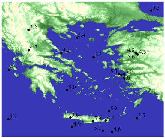
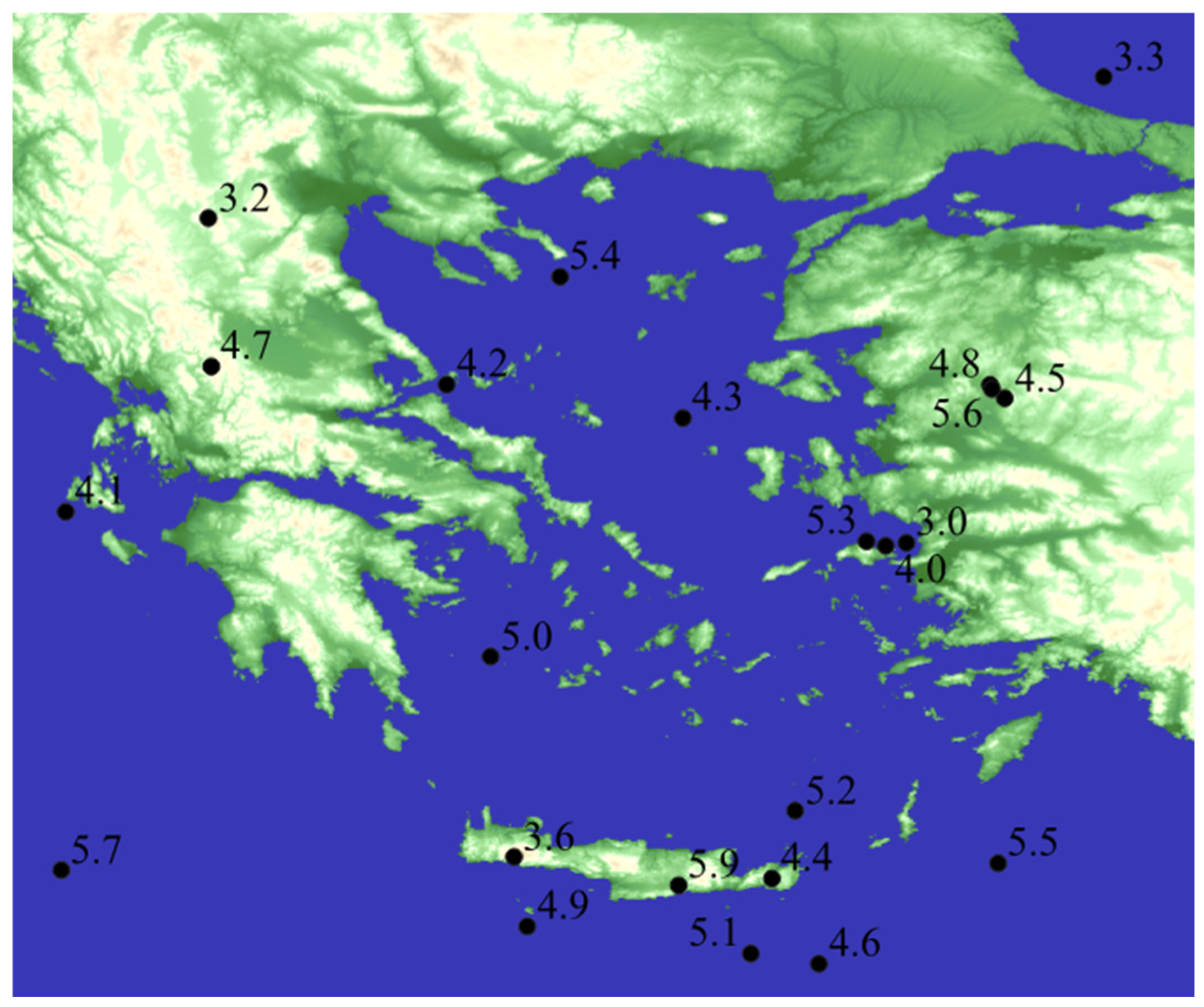
The area under investigation is provided in Figure 1, showing the 23 earthquake epicenters and their magnitude. The earthquakes’ time and date and the exact coordinates of their epicenters are included in Table 1. Most of the earthquakes belong to Greek territory, while others are in the neighboring area, in Turkey. The earthquakes are distributed on the map in relative proportionality to the seismogenicity of the geographic areas. Earthquakes have also been selected to span the maximal possible magnitude range for the year 2020.

Figure 1. The epicenters marked with black dots and magnitudes marked with black numbers of 23 earthquakes used in this work.

Table 1. A list of the 23 earthquakes used in this study. Latitude and longitude are in decimal degrees ranging from 0° to 180°. The timestamp is in Coordinated Universal Time (UTC) format, with the date at the beginning and the time in hours, minutes and seconds, with the letters ‘T’ and ‘Z’ indicating the UTC format.

No.	Date and Time	Latitude	Longitude	Magnitude	Scale	Location
1	2020-05-11T09:33:07.394Z	37.824	27.144	3.0	ml	10 km WSW of Kusadasi
2	2020-06-01T23:15:01.842Z	40.459	21.483	3.2	ml	7 km WSW of Emporio
3	2020-04-13T23:56:37.740Z	41.603	28.747	3.3	ml	33 km N of Durusu
4	2020-02-20T00:32:32.386Z	35.272	23.962	3.6	mb	17 km WNW of Chora Sfakion
5	2020-10-30T12:41:31.954Z	37.797	26.977	4.0	mb	4 km N of Samos
6	2020-04-18T23:36:53.658Z	38.073	20.321	4.1	mb	17 km SW of Lixouri
7	2020-10-17T20:31:59.067Z	39.108	23.415	4.2	mb	8 km SW of Skiathos
8	2020-07-07T15:19:51.452Z	38.836	25.331	4.3	mb	38 km NNW of Psara
9	2020-06-04T04:51:18.397Z	35.089	26.052	4.4	mb	14 km SSW of Sitia
10	2020-02-04T16:47:10.864Z	38.997	27.941	4.5	mb	12 km NE of Akhisar
11	2020-10-30T09:20:36.917Z	34.401	26.428	4.6	mb	89 km S of Palekastro
12	2020-02-06T09:24:16.857Z	39.254	21.497	4.7	mwr	10 km SSE of Anthiro
13	2020-02-18T16:09:23.758Z	39.107	27.817	4.8	mb	12 km E of Kirkagac
14	2020-12-29T08:06:09.922Z	34.709	24.069	4.9	mb	14 km S of Kastri
15	2020-08-17T07:27:02.373Z	36.897	23.770	5.0	mww	56 km SSE of Hydra
16	2020-05-22T03:40:30.610Z	34.483	25.886	5.1	mww	60 km SSE of Ierapetra
17	2020-10-12T04:11:27.566Z	35.644	26.246	5.2	mww	49 km N of Palekastro
18	2020-10-30T15:14:55.887Z	37.831	26.822	5.3	mww	8 km NW of Kokkari
19	2020-09-26T22:50:25.082Z	39.984	24.334	5.4	mww	31 km SSE of Karyes
20	2020-01-28T15:38:34.436Z	35.218	27.891	5.5	mww	69 km ESE of Karpathos
21	2020-01-22T19:22:16.298Z	39.072	27.838	5.6	mww	15 km ESE of Kirkagac
22	2020-05-20T23:43:16.920Z	35.159	20.277	5.7	mww	224 km SW of Methoni
23	2020-09-18T16:28:17.575Z	35.036	25.303	5.9	mww	12 km SSE of Arkalochori

The pre-seismic ground dislocations can be explained by the dilatancy–diffusion hypothesis, which proposes that stress accumulates in the crustal plates, causing the creation of their cracking before the main rupture of the tectonic plates [37]. As the magnitude of the stress approaches a certain level, fluid migration results in surface displacements [38]. The magnitudes of earthquakes examined in this work are below Mw 6, and therefore, the rupture dynamics are predominantly self-similar, with the ruptures confined within the seismogenic thickness of the plate and their length proportionate to their width [39]. The empirical Mw 4.6 threshold is adopted to separate the two classes of earthquake magnitude, since according to Yen and Ma [40], at this magnitude, the rupture size starts to approach the full seismogenic thickness, and gradual horizontal propagation of the rupture starts. Consequently, earthquakes above Mw 4.6 increasingly acquire different rupture characteristics, engaging larger crustal mass and density, greater ruptures with lateral propagation and greater energy release [41]. As indicated in Table 1, the dataset comprises 23 earthquakes, with 11 of them belonging to the lower magnitude class (Mw ≤ 4.6) and the rest 12 belonging to the higher magnitude class (Mw > 4.6). Based on this near-equal distribution, no class imbalance issues arise in the classification task.

Limiting our observations to a 64 km² area around the epicenter of each earthquake aims to achieve normalization of data, appropriate for the ML algorithms, by confining them to detect the width, distribution and clustering of the ground dislocations and ignoring their lengths. The models capture these patterns as footprints of the total crustal stress to be released when the event occurs [42].

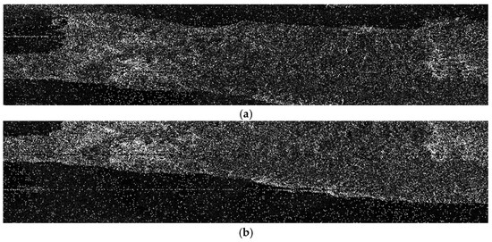
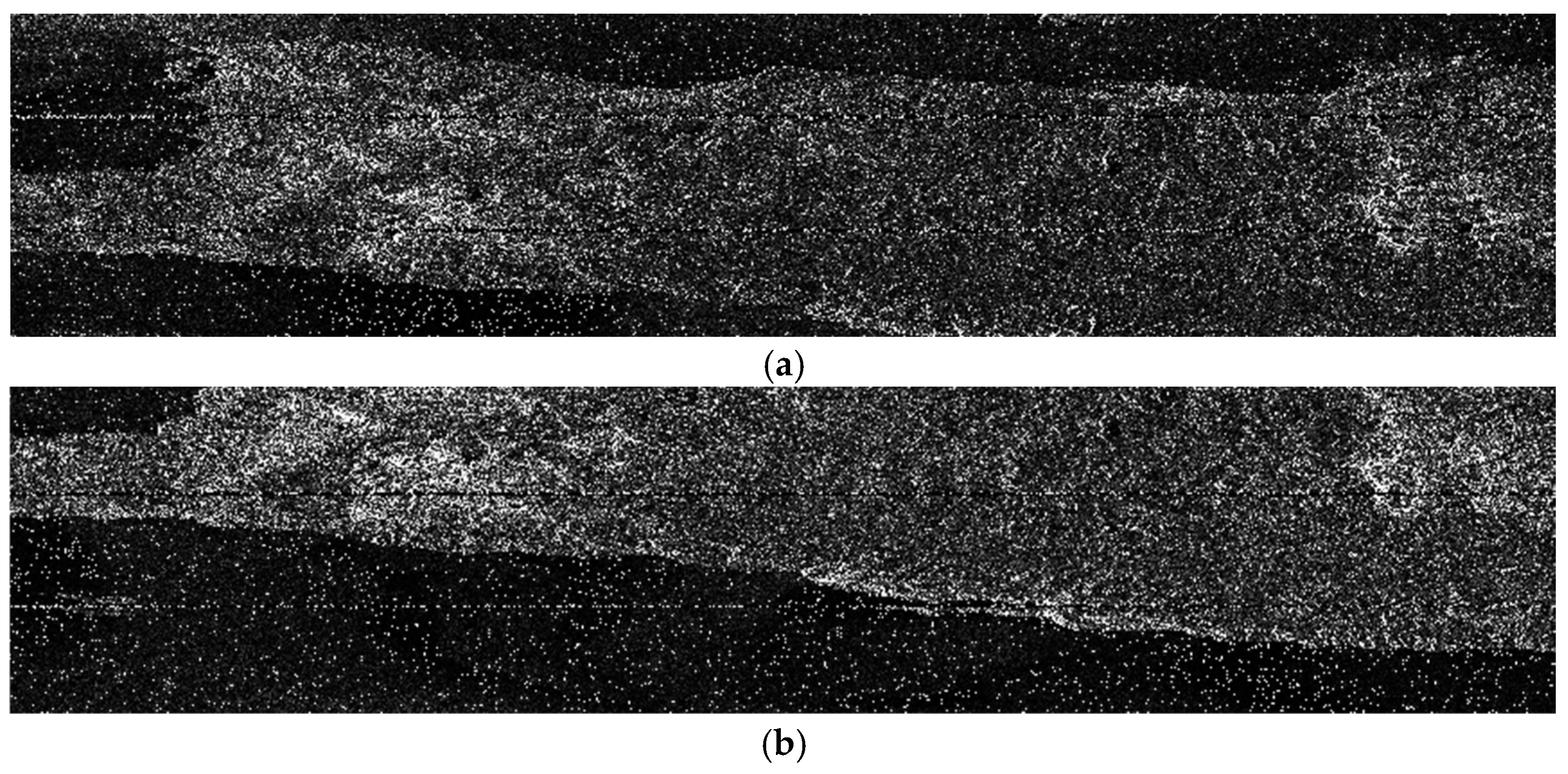
The SAR images were for five six-day intervals before the occurrence of the earthquake. The last image was recorded a couple of hours to four days before the earthquake, depending on the availability of images in the database. Figure 2 illustrates two indicative SAR images, taken on 24 August and 30 August, for the Mw 5.9 earthquake that occurred in Arkalochori, Crete, on the 18 September 2020. Horizontal lines are due to the bursts of the satellite SAR sensor, while the covered area is not exactly the same in the two images, since it depends on the satellite orbit on the acquisition date. Yet, in both SAR images, the epicenter of the earthquake is located on the middle vertical line of the image.

Figure 2. Intensity of reflected SAR radiation on (a) 24 August 2020 and (b) 30 August 2020, referring to Arkalochori, Crete earthquake.

InSAR was employed to generate four interferograms for each earthquake from the five SAR images, using the Sentinel Application Platform (SNAP) Sentinel Toolbox of the European Space Agency [43] and according to the instructions provided by the ESA [44]. Three bursts of the first sub-swath (IW1) of the Interferometric Wide (IW) swath mode, covering the earthquake epicenter and vertical–vertical (VV) polarization, were used. Except for cases involving unusual weather conditions, the average atmospheric delay effect is less than 20 mm [45]. Therefore, atmospheric artifacts were not explicitly corrected; yet their expected magnitude (<20 mm under typical conditions) is substantially lower than the deformation amplitude observed in the used dataset. The latter is acknowledged as a limitation, but it should be noted that it does not affect the objective of evaluating whether pre-seismic deformation contains discriminative information. Figure 3 illustrates the phase difference image resulting from the process above for the two SAR images in Figure 2.

Figure 3. Phase differences image generated from SAR images on 24 August and 30 August 2020, referring to Arkalochori, Crete earthquake. Colors encode wrapped phase (0–2π), where repeating color cycles indicate equal increments of ground displacement.

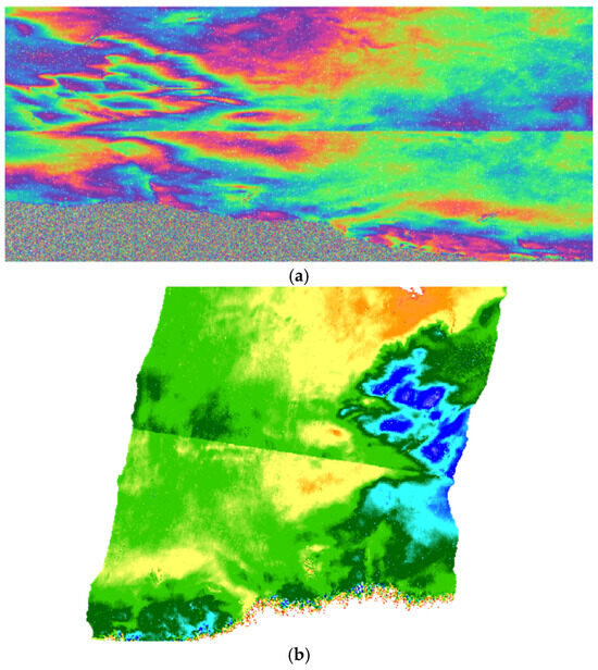
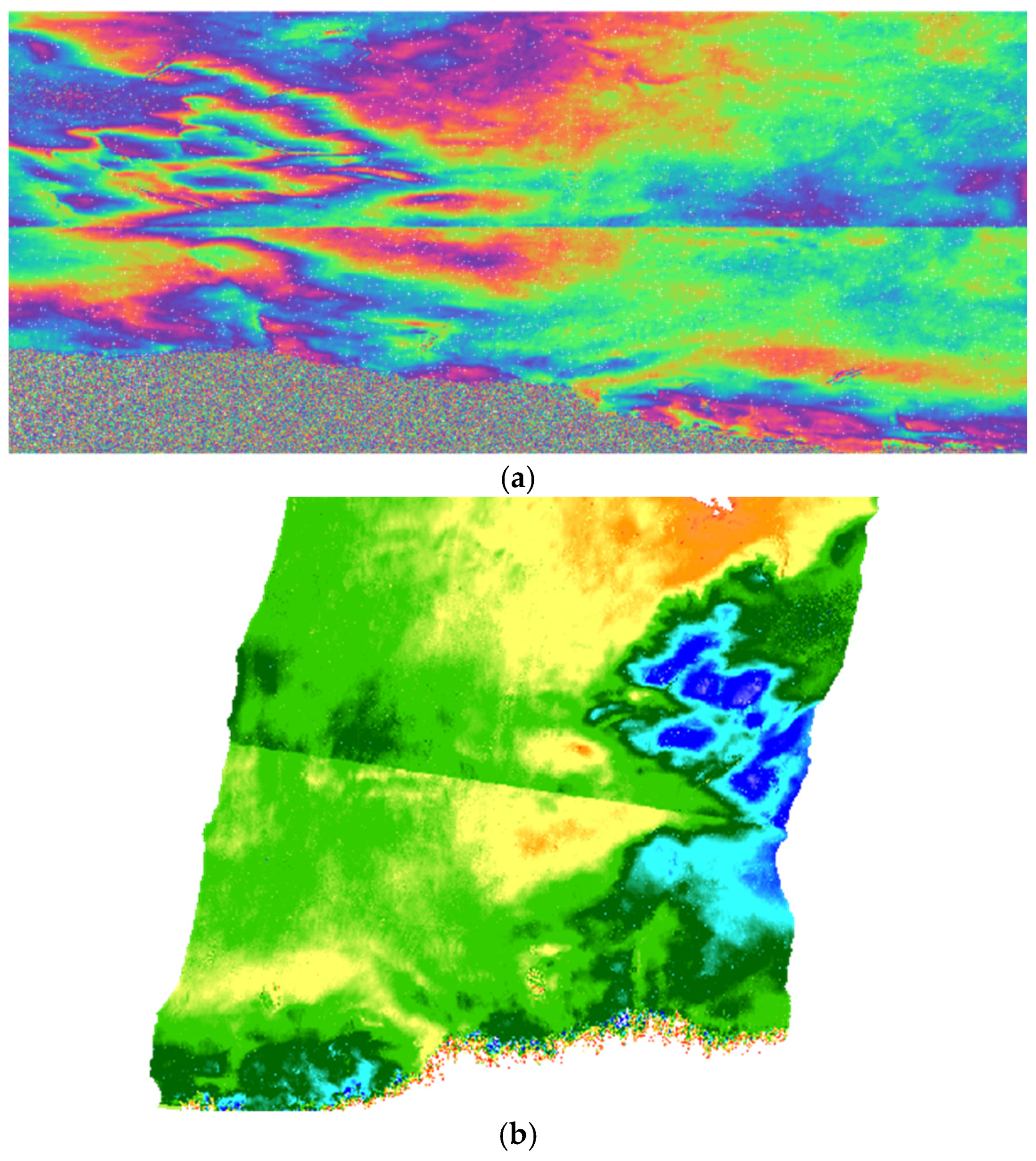
All dislocation images were cropped into 100 × 100-pixel-size rectangles with the epicenter of each earthquake in their center, as shown in Figure 4a. After phase unwrapping to resolve interferometric phase ambiguity, phase differences were converted into ground displacements in meters and were geographically corrected through terrain correction. Thus, a single color image, namely the original image, was generated for each earthquake, showing the total ground displacement during the 24–28-day period before the earthquake, as illustrated in Figure 4b.

Figure 4. (a) A ground dislocation cropped image containing the epicenter of the Arkalochori, Crete earthquake where colors denote wrapped phase (0–2π), with repeating color cycles marking displacement fringes, and (b) the resulting ground dislocation RGB image where the red, green, and blue channels represent the three wrapped-phase components.

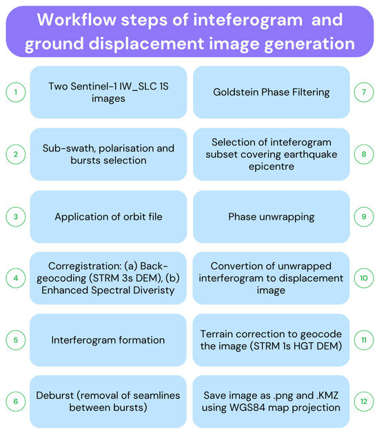
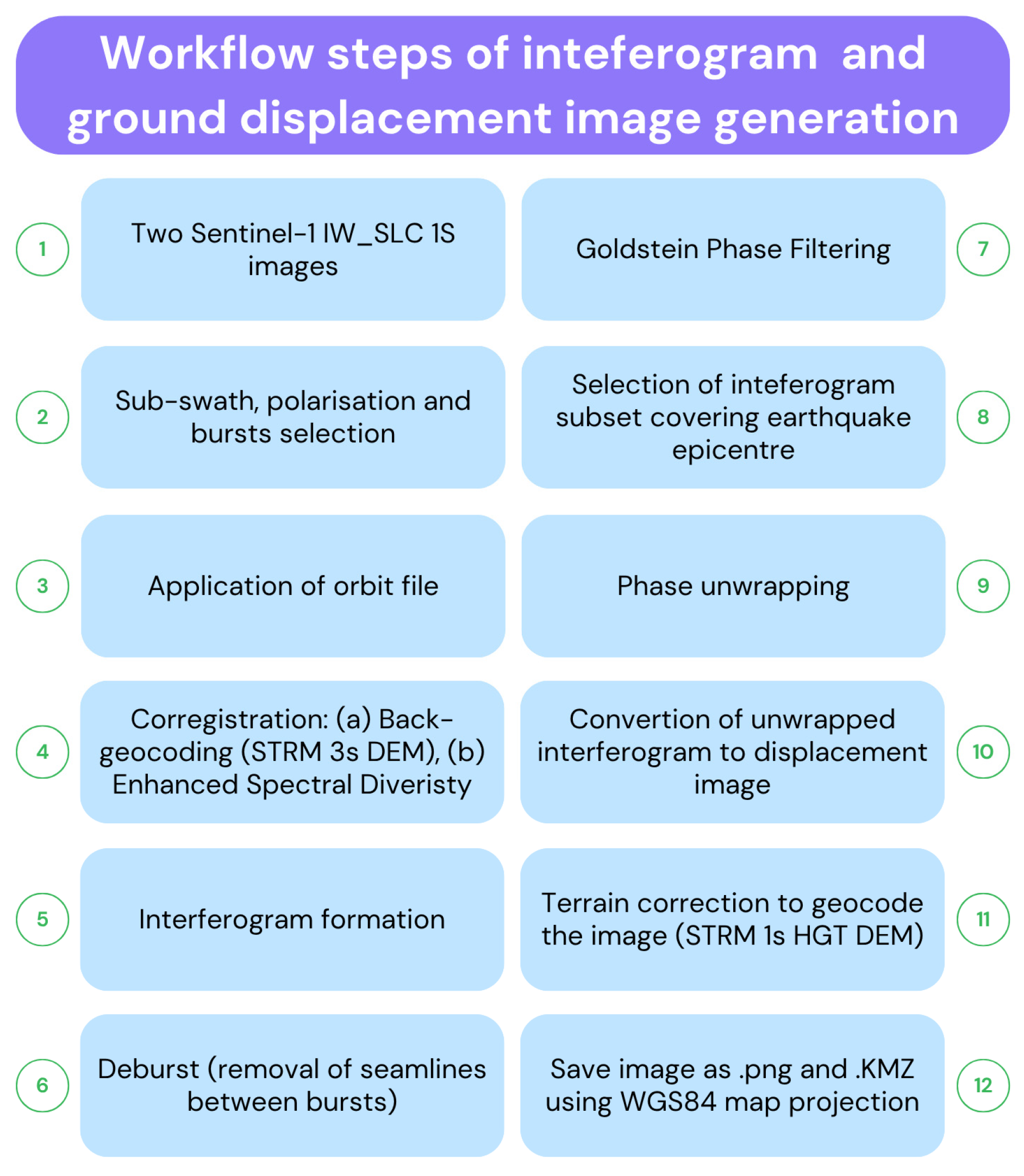
Ground displacement images, in .png and .kml format, were generated from the InSAR interferograms. The detailed workflow for the interferogram and ground displacement image generation methodology is provided in Figure 5.

Figure 5. Workflow for interferogram and ground dislocation image generation.

Fusion was performed by employing the wavelet fusion methodology or by simple addition of the four original dislocation cropped images as arrays, after scaling them to avoid overflow of the pixel values above 255. For the wavelet fusion, the original non-fused color images were first converted into 100 × 100 × 3 three-dimensional (3D) numpy arrays. For each of the four images of an earthquake, the array layer for the same color was converted into a waveform (wavelet transform). The four sets of wavelets for the same color, each one derived from one of the four original non-fused images, were added using the average of their amplitudes into a single layer that was then min-max-normalized. The three resulting fused normalized layers, one for each color, were then stacked into a 3D array for each earthquake.

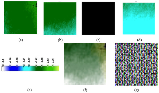
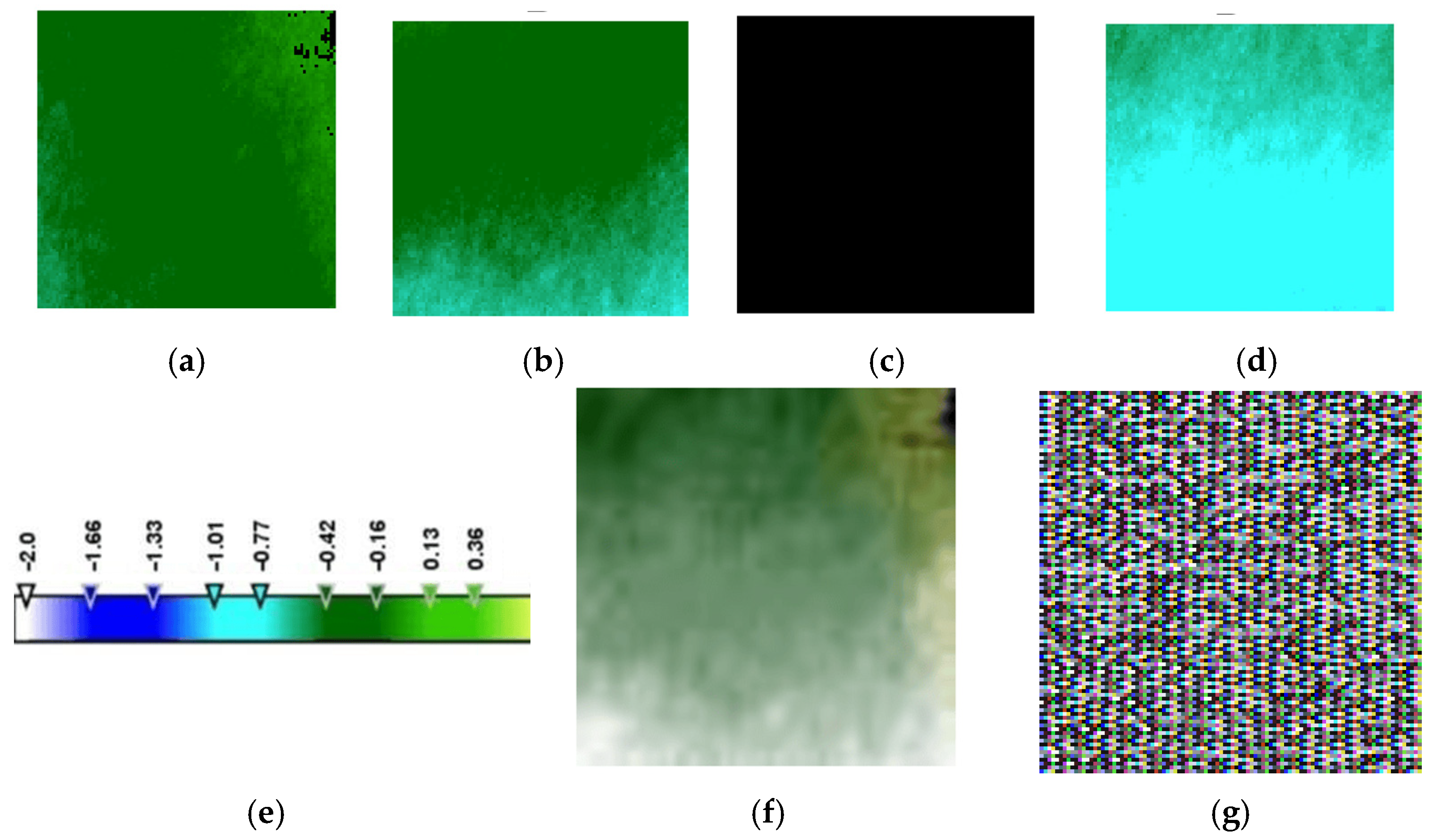
Fused images produced with the use of the wavelet method are referred to in the text as ‘wavelet-fused’ while the images produced by the simple addition of the array forms of the four separate ground dislocation images are referred to as ‘added’. An example of the ground dislocation images is given in Figure 6 for the earthquake of Mw 5.0. The extent of dislocation is shown by the appropriate color, according to the color scale included in the figure. A wavelet-fused image and an added fused image showing the total dislocation during a 24-day period before the earthquake are also provided. It must be emphasized that each dislocation is calculated from two satellite SAR images taken at the beginning and the end of each six-day period. Transient movement in between ground movements cannot be detected.

Figure 6. Ground dislocation images before the Mw 5.0 earthquake, cropped to 100 × 100 pixels around the earthquake epicenter during six-day time intervals, on (a) 24 to 30 July, (b) 30 July to 5 August, (c) 5 to 11 August (total black image indicates no net ground movement during that time period), and (d) 11 to 17 August. (e) The color scale to provide the extent of dislocation relative to the satellite position in meters. (f) Wavelet-fused image and (g) fused added image, referring to the total ground dislocation image for the entire 24-day time period from 24 July to 17 August, both derived from images (a–d). Negative values of ground dislocations represent earth uplifting or/and horizontal slipping towards the satellite position.

First and second-order time derivatives of the ground movement process were also produced. A recent work by Chariskou et al. [46] employed the derivatives of gravity and correlated them to earthquake magnitude, also motivating their adoption into the proposed methodology. In this approach, the four grayscale cropped dislocation images for each earthquake were used. For each pixel, its value derivatives were calculated from the earliest image to that closest to the day of the earthquake. First-order derivatives show the speed of ground dislocations around the earthquake epicenter over time. Second-order derivatives represent the acceleration of the dislocation, the rate at which this speed changes. Specifically, the four values for each pixel, corresponding to one value on each image, were used to calculate four derivatives, each one stored in one of the four layers of the third dimension of the 3D array. In other words, the 3D array had a size of four pixels in its third dimension, and each pixel stored the value of one of the four derivatives.

The cropped images were divided into two classes. One class comprised smaller earthquakes of magnitude 3.0 to 4.6 Mw, and the other contained larger earthquakes of 4.7 to 5.9 Mw. The latter threshold is the statistical median of the dataset, also referring to a magnitude area of 3 to 5 Mw, above which significant damage to structures can occur [47]. Magnitudes reported in scales other than Mw were converted to the Mw scale. In general, magnitude-scale conversions introduce inherent uncertainty, particularly for smaller events where empirical relationships are less stable. This issue is addressed by using the equations of Burton et al. [48] and Lolli et al. [49] and the accepted direct equivalence of the Mwr scale to Mww. Importantly, none of the converted values crossed the Mw = 4.6 threshold used to define the two magnitude classes. Therefore, although conversion uncertainty exists, it does not affect class membership for any of the 23 earthquakes and consequently does not influence the classification results.

The final number of data types used in this work are summarized in Table 2.

Table 2. Number of images of each data type, resulting from all 23 earthquakes.

SAR	InSAR	Dislocation	Fused	First-Order Derivatives	Second-Order Derivatives
115	92	92	23 × 2 (two fusion methods)	23	23

2.2. Epicenter Determination

Using the ruler tool of Google Earth Pro on the .kmz images transferred to it, it was calculated that images cropped to 100 × 100-pixel size correspond to a square geographic area of sides of approximately 8 km (8 × 8 km area), with the earthquake epicenter located at the meeting point of its diagonals. This image size corresponds to a geographic area of about 64 km² around the epicenter.

Two different dislocation groups were defined in each image: one with pixel values below the average (low-displacement group) in the image and the other containing pixels with values higher (high-displacement group) than the average. In most cases, these groups were not continuous, but each one of them consisted of a number of disconnected areas. The epicenter location was defined in relation to the middle of the line joining the centroids (‘centers of gravity’) of the two dislocation groups.

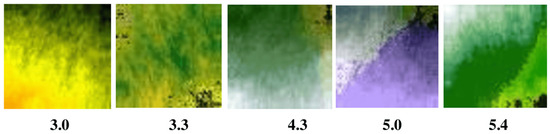
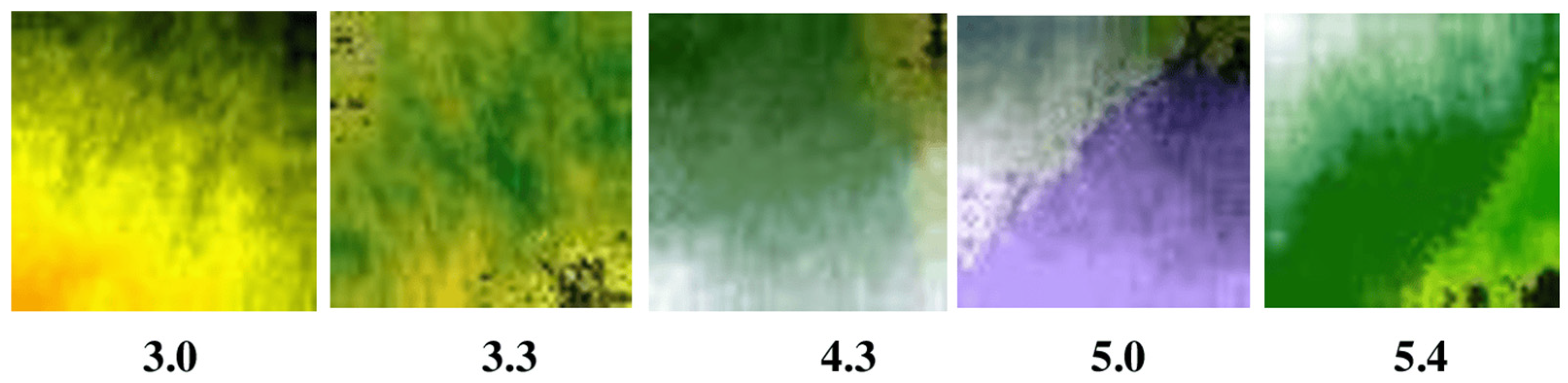
It should be noted here that through the examination of the wavelet-fused color images of pre-seismic ground dislocations, it was observed that the epicenter was located in a belt between two separate dislocation areas. This observation motivated the formulation of epicenter localization as a one-dimensional regression problem, aspiring to locate the epicenter relative to the two main dislocation groups. For this reason, only wavelet-fused images are considered for epicenter localization, since they consistently enhance the separation between the two deformation groups, making the centroid-based geometric representation more stable. Indicative wavelet-fused images are presented in Figure 7. The regression target was defined as the signed distance of the true epicenter from the midpoint of the centroid-to-centroid axis, measured in pixel units.

Figure 7. Wavelet-fused images of ground dislocations of selected earthquakes. Magnitudes are shown below each image. The images have been cropped in a way that the epicenter is located at the middle (intersection of diagonals) of the rectangular frame. It can be discerned that the epicenter is positioned between two major dislocation groups in most earthquakes, separated by the diagonal of the image. Colors encode the fused multiscale deformation components, with hue and brightness reflecting the relative amplitude and spatial structure of ground dislocation.

2.3. Machine Learning for Magnitude Class Prediction

Three different machine learning algorithms were used for predicting the earthquake magnitude, all implemented in Jupyter Notebook 7.5.1. environment: (1) an SVM involving a statistical ANOVA test step, (2) an RF with ANOVA, and (3) a CNN (MobileNetV2. The selection of these three models is based on their complementary strengths and aims to ensure a balanced methodological framework, considering the fact that SVM is a strong baseline effective for small datasets [50], such as in our case, RF with ANOVA combine ensemble robustness with dimensionality reduction for noisy geophysical features [51], and CNN provides a deep learning benchmark for exploiting spatial structure in InSAR images [16]. The ANOVA approach keeps the 100 features showing statistically significant differences between small and large seismic events. Thus, it keeps the features with the most predictive value instead of those with the most variance. Through this selection approach, this work is able to compare classical machine learning with deep learning approaches to test the robustness of the proposed approach across different feature representations, e.g., raw images, fused images, and derivatives, and to ensure that the experimental findings are not model-dependent, but could generalize, reflecting genuine pre-seismic patterns. Table 3 lists the main features of the three selected algorithms used in this work. To avoid data leakage for the case of the original image dataset, where there are four images per earthquake event, the Leave-One-Event-Out Cross-Validation (CV) strategy was used. Standard 3-fold CV was employed in all remaining cases of fused images and derivatives, since in these cases, one sample per event was available.

Table 3. A list of the main features of SVM, RF and CNN classification models used in this study.

Model Setup	SVM	RF	CNN
Preprocessing	RobustScaler, flattening.	RobustScaler, flattening.	Data resize to (150, 150, 3) and normalization to [0, 1].
Additional process	Statistical selection (SelectKBest, k = 100) using ANOVA F-value.	Statistical selection (SelectKBest, k = 100) using ANOVA F-value.	Training data augmentation dynamically on the fly per batch, generating new samples at each epoch.
Model parameters	Balanced class weights. Parameter optimization: GridSearchCV ‘C’: [0.1, 1, 10, 100], ‘gamma’: [0.0001, 0.001, 0.1, 1], ‘kernel’: [‘rbf’, ‘poly’]	Balanced class weights. Threshold scanning from 0.0 to 1.0 in 100 steps to maximize small-class F1.	MobileNetV2 base (frozen initially) + GAP + Dense (128, ReLU) + Dropout (0.5) + Dense (2, Softmax)
Optimization	-	Optimization Criterion: Highest F1 score for small earthquake class.	Optimizer: Adam, Loss: categorical_crossentropy Callbacks: Early Stopping including ReduceLROnPlateau.
Evaluation strategy	Leave-one-out for original images, 3-fold CV for a fused images and derivatives.	Leave-one-out for original images, 3-fold CV for a fused images and derivatives.	Leave-one-out for original images, 3-fold CV for a fused images and derivatives.
Evaluation metrics	Accuracy, precision, recall, F1-score, and confusion matrices.	Accuracy, precision, recall, F1-score, and confusion matrices.	Accuracy, precision, recall, F1-score, and confusion matrices.

Special adaptations were necessary in the case of the derivatives used as inputs to the prediction models. Specifically, in the case of SVM and RF, the derivatives were in the form of three-dimensional (3D) arrays with four temporal layers along the third dimension, each representing the temporal derivative of ground dislocation between consecutive images, thereby encoding the evolution of pre-seismic movements over time. SVM and RF operate directly on ANOVA-reduced derivative vectors. However, MobileNetV2 requires three input channels (arrays with only 3 layers). It was necessary, therefore, to remove the most distant time-wise layer, i.e., the earliest temporal layer, retaining the three layers containing the most relevant pre-seismic information of the derivatives closer to the time of the earthquake.

The same pre-trained MobileNetV2 was used for image and derivative array processing. Due to the limited size of the dataset, data augmentation was employed in this case to improve predictions. Training was performed for 70 epochs. Each epoch used one batch of 32 images or arrays, all dynamically on-the-fly augmented from the original training images or arrays by rotation, shifting, zooming and flipping. Each epoch generated a new augmented batch, thus ensuring that the model was exposed to a large variety of transformed samples. The added, wavelet-fused and derivative datasets used 16 images or arrays for training. Even though we used arrays in the case of the derivatives instead of images, these are treated as numerical grids, and the generator modified the numbers according to the grid transformations requested in the augmentation. Therefore, a final set of 70 × 32 = 2240 images or arrays were used for training the model, all of them augmented. In the case of the original images, there were 64 images for training. Ninety-six (96) augmented images were used in 3 batches of 32 for each of the 70 epochs of the code. Therefore, a total of 70 × 96 = 67,200 images were used for training.

Feature extraction to convert the interferometrically derived ground dislocations into physical variables was implemented. Specifically, the kinematics of pre-seismic dislocation were analyzed by using first and second-order derivatives, instead of static data. Temporal derivatives can capture the kinematics of pre-seismic deformation, e.g., rate and acceleration. Wavelet fusion was then used to spatially filter the raw data by isolating the earthquake-related dislocation patterns from noise. During wavelet fusion and general decomposition–recomposition of images or arrays, the images or arrays are decomposed into frequency sub-bands. Thus, wavelet fusion enhanced coherent deformation patterns by decomposing images into frequency sub-bands and recombining them. Finally, dimensionality reduction was employed by using ANOVA to produce a limited number of orthogonal components that capture and emphasize the most important image features related to the ground dislocations, as well as to remove noise uncorrelated to them.

2.4. Machine Learning for Epicenter Localization

Five different regression models, SVR, RF, CNN, MLR and PLS, were used to predict the distance of the earthquakes’ epicenters from the midpoint of the axis joining the centroids of the two ground dislocation groups in each image. The algorithms were used as inputs the 23 wavelet-fused RGB images showing the total ground displacement around the epicenter of each of the 23 earthquakes for the entire period of 24 days before the earthquake. Each image represented an earthquake of different magnitude. All algorithms included the same initial steps, consisting of converting the images to grayscale and resizing them to a 64 × 64-pixel size, dividing the image pixels into two groups of values above and under the average for each image pixel value, finding the centroid of each group, and calculating the true distance of the epicenter from the midpoint of the axis joining the two centroids. The features of the models used are summarized in Table 4. Data augmentation, generated on the fly during each batch formation, was used in the case of the CNN.

Table 4. A list of the main features of SVR, RF, CNN, MLR and PLS regression models used in this study.

Model Setup	SVR	RF	MLR	PLS	CNN
Preprocessing	Flatten the images and normalize the values.
Data split	3-fold cross validation
Additional process	Train the model using the best parameters. Fit the test set to predict distances of the epicenters from the axis midpoint.
Model parameters	Use Run Support Vector Regression to find the best paraments of the GridSearchCV parameter grid: C: [0.1, 1, 10] epsilon: [0.01, 0.1, 0.2] kernel: [‘linear’, ‘rbf’] Use 3-fold CV and neg_mean_squared_error.	Use RandomForestRegressor to define the best parameters of the GridSearchCV Param grid: n_estimators, max_depth, min_samples_split, min_samples_ 3-fold cross-validation Scoring: negative MSE.	Model: LinearRegression.	PLS regression with for GridSearchCV tuning, n_components (1–10). Scoring: neg MSE.	ResNet50V2 on the fly data augmentation per epoch: RandomFlip, Rotation, Zoom. Conv2D + MaxPooling Flatten + Dense layers Output: 1 neuron Loss: MSE Optimizer: Adam. 3-fold CV.
Evaluation metrics	MAE, RMSE, R2 score Ground dislocation images showing the epicenter location, the centroid positions and the axis joining them, and the predicted distance of the epicenter from the midpoint of the axis.

3. Results and Discussion

3.1. Magnitude Class Prediction

The accuracy results of the prediction of magnitude class for all three models and different image types are given in Table 5. Accuracy depends greatly on the type of prediction model and the data used. The best accuracies were obtained with the RF and first- and second-order derivatives.

Table 5. Performance metrics of earthquake magnitude classification for SVM, RF and CNN models. Highest performances were obtained with second derivatives of ground dislocations with RF model.

Magnitude Class:	≤4.6 mw (Small, 11 Events)			>4.6 mw (Large, 12 Events)
Data type:	Original
Model	Precision	Recall	F1-Score	Precision	Recall	F1-Score	Accuracy
SVM	0.000	0.000	0.000	0.520	1.000	0.684	0.520
RF	0.818	0.188	0.305	0.562	0.962	0.709	0.590
CNN	0.368	0.146	0.209	0.494	0.769	0.602	0.470
Data type:	Added
SVM	0.357	0.417	0.354	0.583	0.417	0.417	0.423
RF	0.557	0.917	0.687	0.889	0.333	0.457	0.607
CNN	0.500	1.000	0.665	0.333	0.083	0.133	0.518
Data type:	Wavelet fused
SVM	0.244	0.250	0.243	0.378	0.417	0.392	0.345
RF	0.500	1.000	0.665	0.333	0.083	0.133	0.518
CNN	0.083	0.083	0.083	0.440	0.750	0.548	0.440
Data type:	1st-order derivatives
SVM	0.583	0.611	0.583	0.617	0.583	0.583	0.607
RF	0.756	0.806	0.778	0.806	0.750	0.774	0.780
CNN	0.222	0.333	0.267	0.690	0.833	0.687	0.607
Data type:	2nd-order derivatives
SVM	0.743	0.917	0.811	0.667	0.583	0.619	0.750
RF	0.833	1.000	0.889	0.667	0.667	0.667	0.833
CNN	0.500	0.417	0.422	0.579	0.750	0.620	0.607

The second-order derivatives represent the acceleration of the ground dislocations. It can be assumed, therefore, that the acceleration of dislocations is related to earthquake magnitude. This outcome is anticipated, since speed is related to momentum and therefore to the tectonic plate percussion-related strain.

More analytically, the results of Table 5 overall demonstrate that raw pre-seismic displacement images contain limited discriminative information for magnitude classification, with all models performing poorly on the original data. Specifically, SVM reports zeros in all metrics for the small magnitude class. The latter can be attributed to the fact that original raw inputs contain insufficient discriminative information for separating the magnitude classes. The high dimensionality and low structural content of the displacement data prevent SVM from learning a meaningful decision boundary, causing the model to collapse in the small magnitude class while only predicting the large magnitude class. The latter limitation disappears when derivative-based representations are used, confirming that magnitude-related information is encoded in deformation dynamics rather than in statistical displacement values.

As can be observed, therefore, performance substantially improves when fused or derivative-based representations are used. Specifically, second-order derivatives reported the highest accuracies across most of the models, indicating that acceleration of pre-seismic deformation is more informative compared to absolute displacement values.

CNN benefits from fused images, while classical ML models such as SVM and RF rely on structured derivative features. Experimental findings suggest that magnitude-related information is encoded primarily in the temporal evaluation of pre-seismic deformation, rather than in static displacement fields.

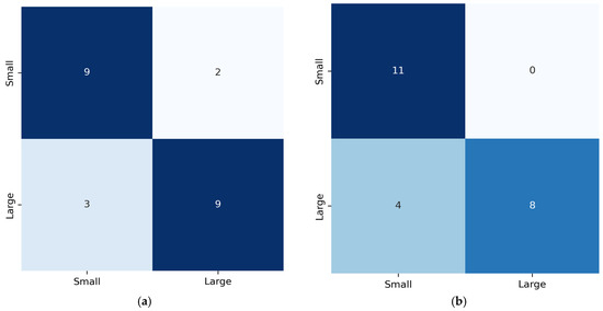
Confusion matrices for the best accuracies reported for the cases in Table 5 (RF with second-order derivatives and RF with first-order derivatives) are presented in Figure 8, aiming to offer class-level insights that accuracy alone cannot provide.

Figure 8. Confusion matrices of earthquake magnitude prediction from best-performing model, RF: (a) using first-order derivatives; (b) using second-order derivatives. Color intensity reflects the number of samples in each cell, with darker colors indicating higher counts.

More analytically, by using first-order derivatives, the model achieves well-balanced classification results, identifying nine small and nine large events. In contrast, second-order derivatives reported perfect recall for small magnitude classes (11 out of 11), indicating that acceleration patterns characterize weaker events. Yet a slight increase is observed in confusion for the large magnitude class, where four events are misclassified as small. Overall, both confusion matrices confirm that derivative-based representations are capable of capturing the most discriminative pre-seismic deformation features, with first-order derivatives offering balanced performance and second-order derivatives enhancing sensitivity to small events.

3.2. Epicenter Correlation to Surrounding Ground Dislocations

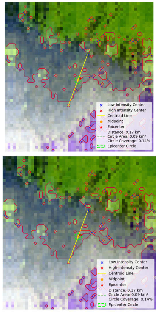
Table 6 includes the true distances of the earthquake epicenters from the middle point of the axis joining the centroids of the two major ground dislocation groups. An indicative example of the predicted location of the epicenter of the mb 4.6 earthquake event is shown in Figure 9.

Table 6. The true distances of the earthquake epicenter from the middle point of the axis joining the centroids of the two major ground dislocation groups. For the Mw 5.2 earthquake, no discrete ground dislocation groups could be identified.

Magnitude (Mw)	Distance (km)
3.0	0.13
3.2	0.10
3.3	0.10
3.6	0.96
4.0	0.67
4.1	0.20
4.2	0.49
4.3	0.14
4.4	0.04
4.5	0.33
4.6	0.10
4.7	0.09
4.8	0.61
4.9	0.06
5.0	0.21
5.1	0.11
5.2	1.78
5.3	1.78
5.4	0.25
5.5	0.08
5.6	0.12
5.7	0.09
5.9	0.27
Average distance:	0.378 km

Figure 9. An indicative example of the localization of the epicenter of an earthquake in relation to the middle point of the yellow line joining the centroids of two major ground dislocation groups. The two dislocation groups are defined by their border line (red line). The distance of the epicenter (red star label) from the middle point is given in km as shown in the legend, and in this case, it is 170 m. The periphery of the green circle shows the potential predicted points of epicenter localization. The side of the square image is about 8 km.

The complete regression results of the prediction of the epicenter distance from the centroid axis midpoint are summarized in Table 7. The “average predicted distance” included in Table 7 refers to the mean of the predicted distances of the epicenters from the midpoints of the axes joining the centroids of the two-pixel groups in each image. That is the average of 22 such predicted values (after removing Mw 5.2 earthquake), since the 3-fold validation ensured that all 22 images were included in the test set exactly once. Specifically, the Mw 5.2 event was removed before CV, and the remaining 22 events were then split into training and testing sets within each fold. Since a three-fold CV was applied to the dataset of 22 samples, the first two folds contained seven test images each, while the third fold contained eight, ensuring that all 22 events were used exactly once for testing. The experimental findings demonstrate that the spatial configuration of pre-seismic ground dislocation clusters probably contains meaningful information regarding epicenter location.

Table 7. Evaluation metrics of the prediction of the distance of the earthquake epicenter from the midpoint of the axis joining the centroid of the two ground dislocation groups using five ML regression models. The percentage of earthquakes with their predicted epicenter distance from the true epicenter location within 300 m and 500 m is also calculated.

Regression Method	Average Predicted Distance (km)	MAE	RMSE	R2 Score	Accuracy Within ± 500 m	Accuracy Within ± 300 m
Images with epicenter located at image center
SVR	0.355	0.261	0.415	0.876	84%	76%
RF	0.301	0.186	0.237	0.716	100%	73%
CNN	0.300	0.159	0.216	0.765	95%	82%
MLR	0.332	0.360	0.413	0.139	78%	47%
PLS	0.277	0.328	0.401	0.190	82%	52%
Images with epicenter at position 25% downward and leftward relative to image center
SVR	1.962	0.165	0.239	0.138	91%	82%
RF	1.921	0.136	0.218	0.286	91%	82%
CNN	2.040	0.235	0.312	−0.458	86%	69%
MLR	1.937	0.180	0.246	0.092	91%	82%
PLS	1.922	0.160	0.222	0.260	95%	82%

Moreover, Table 7 includes the percentage of earthquakes that predicted epicenter distance from the true epicenter location within a predefined distance (±300 m and ±500 m), based on the following formula:

$${Acc}_{distance}\left(\%\right)={\displaystyle \frac{1}{22}}{\displaystyle \sum _{i=1}^{22}}{D}_i\times 100$$

(1)

where $i$ refers to the number of events, and $D_i$ is an indicator function equal to 1 when the absolute difference between the actual ($e_i$) and predicted epicenter ($e_i^{\prime }$) location of the event $i$, i.e., the distance error $|{\mathrm{e}}_{\mathrm{i}}-{\mathrm{e}}_{\mathrm{i}}^{\prime }|$, is smaller or equal to the predefined distance, and 0 otherwise:

$$D_i=\left\{\begin{array}{l}1, \mathrm{if} |{\mathrm{e}}_{\mathrm{i}}-{\mathrm{e}}_{\mathrm{i}}^{\prime }|\le \mathrm{distance}\\ 0, \mathrm{otherwise}\end{array}\right.$$

(2)

In Table 7, the accuracy of predicted distance is calculated for distances of ≤300 m and ≤500 m, indicating the proportion of events for which the predicted epicenter lies within the specified radius of the true location.

When the epicenter is centrally positioned within the 100 × 100-pixel cropped area (~8 × 8 km), the RF and CNN models achieve the best overall performance. RF reports the highest accuracy within ±500 m (100%) and the lowest RMSE (0.237 km), while the CNN achieves the lowest MAE (0.159 km) and a competitive RMSE (0.216 km). Both models also report high R² scores, indicating that they can effectively exploit the spatial structure of wavelet-fused images and can extract fine-grained deformation patterns that correlate with epicenter location.

Considering as an example the RF results, the side of the square image is about 8 km, and therefore, the covered area is about 64 km². Notably, the RF algorithm estimates that 100% of the actual epicenters are expected to be located within a circle of 500 m radius around the estimated point. This is an area representing about 1.2% of the examined 64 km² square. The latter demonstrates a substantial improvement in spatial precision, since the model reduces the search area for the epicenter to less than 0.78 km². Practically, a smaller predicted area means better targeting for hazardous assessment and emergency planning in the case of destructive earthquakes. Instead of monitoring a broader area, the authorities could focus and concentrate their resources on a much smaller zone. The results confirm that the regression models can capture encoded localized geometric signatures of impeding rapture in pre-seismic deformation acceleration.

To assess the robustness of the proposed approach, a second experiment was conducted using images where the epicenter was shifted relative to the image center. This shift aims to disrupt the symmetry of the deformation field and test whether the learned relationships are dependent on image alignment. The experimental results in this case indicate SVR, RF and PLS as the best-performing models. The performance of the CNN decreases in this case, indicating that the CNN is more sensitive to spatial alignment, while classical regression models are more robust to geometric translation.

Using images where epicenters are not at their center produces some interesting results reflected in R² score values; a negative value is reported, indicating a lower correlation of ground dislocations to epicenter location. It is, therefore, concluded that ground dislocations around the epicenter are of a specific type, more related to the earthquake center than dislocations at more distant regions. This reinforces that the relationship between pre-seismic deformation and epicenter position is inherently nonlinear and requires ML models capable of capturing the complex underlying spatial and geometric patterns.

The employment of wavelet fusion and time derivatives enhances the signal-to-noise ratio. The latter also provides information on the stress-loading phase before the rupture. The proven relation of the epicenter to the dislocation patterns around it indicates that the crustal stress is producing localized measurable surface features. The lower RMSE and higher R² scores obtained when the epicenter is centrally located in the examined area indicate that the regression models can recognize signals correlated to the location of an impending earthquake.

According to the self-similarity model of crystal rapture, smaller earthquakes are confined within the seismogenic thickness zone and result in smaller surface dislocations, resulting in weaker and less coherent surface signals. Larger events are associated with larger ruptures expanding laterally within the crustal mass, involving a greater mass, causing higher stress release and more intense and more clustered surface dislocation patterns.

Finally, it is important to notice that the predicted epicenters are not located at a point of maximal ground dislocation, as someone would intuitively expect, but are found between two such elevation areas forming a ground folding. At this point, it should be emphasized that this work does not intend to predict the occurrence of an earthquake; it is an effort to predict its magnitude and its approximate epicenter location. Pilot experimental results provide evidence that ML models have the potential to make short-term predictions from ground dislocation data captured in a time interval of less than a month before the date of the earthquake.

Future work would include more magnitude classes, classification and regression models, and data. Yet it should be noted that dataset enhancement refers to a much larger interferogram set, which requires a great deal of resources to obtain in terms of human labor and computational resources.

4. Limitations and Implications

4.1. Limitations

A limitation of this pilot work is the restricted number of available earthquakes within 24 to 28-day pre-seismic InSAR time-series. Generation of pre-seismic InSAR time-series requires exhaustive processing per event, each involving multiple computationally intensive steps. Thus, producing a high-quality interferogram could require a great amount of time on standard hardware, while the lack of access to high-performance computing resources constrained the number of earthquakes that could be processed within the scope of this work. The small sample size inherently limits the statistical power of the models. Future work will focus on the construction of a larger dataset to ensure more extensive temporal coverage. Therefore, this approach should be interpreted as an explanatory demonstration of feasibility, rather than a generalizable predictive system.

Regarding epicenter prediction, two approaches were investigated, one with the centered epicenter in the image and the other with the epicenter deliberately shifted, aiming to avoid over-interpretation of centered image artifacts and assess the robustness of the proposed approach. The results indicate that the correlation between deformation geometry and epicenter location is not merely a product of image centering but rather reflects a spatial pattern in the pre-seismic dislocation field. These pilot findings indicate a pattern, suggesting that future work could focus on extending the proposed approach to non-centered and larger-area interferograms, enabling a more realistic and operational epicenter localization framework.

It should also be noted that the proposed approach does not explicitly consider tropospheric noise or other atmospheric artifacts included in InSAR images; several components of our methodology already mitigate their impact. Wavelet fusion enhances coherent deformation patterns and suppresses high-frequency noise, while temporal derivatives further reduce static atmospheric contributions, focusing on deformation evolution and not on absolute displacement. Yet the ability of the models to extract consistent predictive features despite this noise suggests that pre-seismic deformations may have a detectable spatial signature.

Finally, in this work, magnitude-scale conversion took place. In general, magnitude conversions introduce an additional source of uncertainty. Therefore, future work will incorporate magnitude-scale uncertainty analysis, especially when expanding the dataset to include more events and additional magnitude classes.

4.2. Implications for Infrastructure Resilience and Environmental Sustainability

The proposed work has direct implications for infrastructure resilience, since it promises to statistically infer the magnitude class of an earthquake and approximate epicenter area based on pre-event ground deformations. The latter can enable targeted deployment of structural monitoring of buildings within high-risk areas, especially when earthquakes of high magnitude are expected, prioritizing the inspection of critical structures such as hospitals, bridges, etc. Thus, the proposed approach could inform risk-informed maintenance planning, as well as emergency preparedness and resources, in areas where most structural hazards might be expected.

From the perspective of sustainability, the proposed approach aims to reduce in the long term the socio-economic impact of seismic disasters. More precise short-term predictions could reduce unnecessary large-scale area evacuations and emergency mobilization, minimizing resource waste and achieving sustainable hazard mitigation.

The high value of satellite images is highlighted; extracted ground deformations, even mixed with atmospheric noise, have the potential to enable ML models to extract valuable spatial patterns. However, as already mentioned, the current approach faces several limitations, therefore, it is not intended to replace operational early warning systems but rather to provide insights into the potential of ground deformation patterns to support data-driven decision-making when used alongside established geophysical analysis.

5. Conclusions

In this work, the predictive potential of pre-seismic ground dislocations derived from InSAR images is investigated in relation to earthquake magnitude classification and epicenter localization.

SVM and RF classifiers reported high classification accuracy by using as input data a set of second-order derivatives of ground dislocations. RF also reports efficient accuracy using first-order derivatives. Regarding epicenter localization, the CNN and RF regression models displayed better results in predicting the sites of the same percentage of epicenters (95% and 100%, respectively) within a small circular area of 500 m radius.

The experimental findings highlight the value of integrating InSAR-derived pre-seismic dislocation patterns with machine learning techniques, paving a promising pathway towards more reliable short-term seismic hazard assessment AI-based tools. While our findings provide encouraging evidence of the potential predictive value of the proposed approach, they also underline the need for a more generalized approach across larger datasets.

Outcomes of this work carry direct implications for both infrastructure resilience and environmental sustainability. The ability to estimate magnitude class and approximate epicenter area from pre-seismic deformation patterns can support targeted inspection and maintenance of critical structures, enhancing seismic awareness in high-risk zones. Moreover, more precise spatial prediction could reduce unnecessary large-scale evacuations and emergency mobilization, contributing towards more sustainable hazard mitigation, through the optimization of resource use and minimizing both socio-economic and environmental impact. Overall, the proposed approach could provide a useful supportive tool for seismic risk management when used alongside established geophysical analysis.

References

- World Health Organization Earthquake Statistics. Available online: https://www.who.int/health-topics/earthquakes#tab=tab_1 (accessed on 23 November 2025).
- Anbazhagu, U.V.; Sonia, R.; Grover, R.K.; Banu, E.A.; Jothikumar, C.; Sudhakar, M. AI and Machine Learning in Earthquake Prediction. In Modern SuperHyperSoft Computing Trends in Science and Technology; IGI Global: Hershey, PA, USA, 2024; pp. 1–32. [Google Scholar]
- Wan, X.Y.; Song, Y.; Lau, T.L. Advances in Deep Learning for Earthquake Monitoring and Forecasting: Techniques, Applications, and Future Directions. In Proceedings of the 2024 IEEE 15th International Conference on Software Engineering and Service Science (ICSESS), Changsha, China, 13 September 2024; IEEE: New York, NY, USA, 2024; pp. 69–73. [Google Scholar]
- Gokhberg, M.B. Earthquake Prediction; CRC Press: London, UK, 2024; ISBN 9781003539339. [Google Scholar]
- Bilic, S.; Külahcı, F.; Bilici, A. Predicting the Unpredictable: Advancements in Earthquake Forecasting Using Artificial Intelligence and LSTM Networks. Geomagn. Aeron. 2024, 64, 760–771. [Google Scholar] [CrossRef] [Scilit]
- Dieterich, J.H. Preseismic Fault Slip and Earthquake Prediction. J. Geophys. Res. Solid Earth 1978, 83, 3940–3948. [Google Scholar] [CrossRef] [Scilit]
- Lior, I.; Rivet, D.; Ampuero, J.-P.; Sladen, A.; Barrientos, S.; Sánchez-Olavarría, R.; Villarroel Opazo, G.A.; Bustamante Prado, J.A. Magnitude Estimation and Ground Motion Prediction to Harness Fiber Optic Distributed Acoustic Sensing for Earthquake Early Warning. Sci. Rep. 2023, 13, 424. [Google Scholar] [CrossRef] [Scilit] [PubMed]
- Meier, M. How “Good” Are Real-time Ground Motion Predictions from Earthquake Early Warning Systems? J. Geophys. Res. Solid Earth 2017, 122, 5561–5577. [Google Scholar] [CrossRef] [Scilit]
- Pairojn, P.; Wasinrat, S. The Prediction of Earthquake Ground Motions by Regression Model. In Earthquakes—Forecast, Prognosis and Earthquake Resistant Construction; InTech: Tokyo, Japan, 2018. [Google Scholar]
- Onyelowe, K.C.; Kontoni, D.-P.N.; Onyelowe, F.K.C.; Kamchoom, V.; Hanandeh, S.; Ebid, A.M.; Ulloa, N.; Moghal, A.A.B.; Vishnupriyan, M. Forecasting Earthquake-Induced Ground Movement under Seismic Activity Using Response Surface. Sustain. Intell. Infrastruct. 2025, 1, 4–18. [Google Scholar] [CrossRef] [Scilit]
- Pepe, A.; Calò, F. A Review of Interferometric Synthetic Aperture RADAR (InSAR) Multi-Track Approaches for the Retrieval of Earth’s Surface Displacements. Appl. Sci. 2017, 7, 1264. [Google Scholar] [CrossRef] [Scilit]
- Zhang, L.; Lu, Z. Advances in InSAR Imaging and Data Processing. Remote Sens. 2022, 14, 4307. [Google Scholar] [CrossRef] [Scilit]
- Alizadeh Zakaria, Z.; Ebadi, H.; Farnood Ahmadi, F. Investigation of the Application of Geospatial Artificial Intelligence for Integration of Earthquake Precursors Extracted from Remotely Sensed SAR and Thermal Images for Earthquake Prediction. Multimed. Tools Appl. 2023, 82, 22853–22870. [Google Scholar] [CrossRef] [Scilit]
- Sönmez, N.; Tokdemir, O.B.; Günaydın, H.M. Artificial Intelligence in Earthquake Disaster Risk Management: A Systematic Review of Applications, Challenges, and Research Gaps. In Intelligent and Fuzzy Systems; Springer: Berlin/Heidelberg, Germany, 2025; pp. 791–807. [Google Scholar]
- Ying, Z.; Congcong, W.; Didier, S.; Chengxiang, Z. Integrating Artificial Intelligence and Geophysical Insights for Earthquake Forecasting: A Cross-Disciplinary Review. arXiv 2025, arXiv:2502.12161. [Google Scholar]
- Liu, X.; Zhang, Y.; Shan, X.; Wang, Z.; Gong, W.; Zhang, G. Deep Learning for Automatic Detection of Volcanic and Earthquake-Related InSAR Deformation. Remote Sens. 2025, 17, 686. [Google Scholar] [CrossRef] [Scilit]
- Mirmazloumi, S.M.; Gambin, A.F.; Palamà, R.; Crosetto, M.; Wassie, Y.; Navarro, J.A.; Barra, A.; Monserrat, O. Supervised Machine Learning Algorithms for Ground Motion Time Series Classification from InSAR Data. Remote Sens. 2022, 14, 3821. [Google Scholar] [CrossRef] [Scilit]
- Delouis, B.; Nocquet, J.; Vallée, M. Slip Distribution of the February 27, 2010 Mw = 8.8 Maule Earthquake, Central Chile, from Static and High-rate GPS, InSAR, and Broadband Teleseismic Data. Geophys. Res. Lett. 2010, 37, L17305. [Google Scholar] [CrossRef] [Scilit]
- Vaka, D.S.; Rao, Y.S.; Bhattacharya, A. Time Series Analysis of the Pre-Seismic and Post-Seismic Surface Deformation of the 2017 Iran–Iraq Earthquake Derived from Sentinel-1 InSAR Data. J. Earth Syst. Sci. 2023, 132, 64. [Google Scholar] [CrossRef] [Scilit]
- Guo, N.; Wu, Y.; Zhang, Q. Coseismic and Pre-Seismic Deformation Characteristics of the 2022 MS 6.9 Menyuan Earthquake, China. Pure Appl. Geophys. 2022, 179, 3177–3190. [Google Scholar] [CrossRef] [Scilit]
- Suresh Krishnan, P.V.; Kim, D.; Jung, J. Subsidence in the Kathmandu Basin, before and after the 2015 Mw 7.8 Gorkha Earthquake, Nepal Revealed from Small Baseline Subset-DInSAR Analysis. GIScience Remote Sens. 2018, 55, 604–621. [Google Scholar] [CrossRef] [Scilit]
- Liu, G.X.; Ding, X.L.; Li, Z.L.; Li, Z.W.; Chen, Y.Q.; Yu, S.B. Pre- and Co-Seismic Ground Deformations of the 1999 Chi-Chi, Taiwan Earthquake, Measured with SAR Interferometry. Comput. Geosci. 2004, 30, 333–343. [Google Scholar] [CrossRef]
- Moro, M.; Saroli, M.; Stramondo, S.; Bignami, C.; Albano, M.; Falcucci, E.; Gori, S.; Doglioni, C.; Polcari, M.; Tallini, M.; et al. New Insights into Earthquake Precursors from InSAR. Sci. Rep. 2017, 7, 12035. [Google Scholar] [CrossRef] [Scilit] [PubMed]
- Nardò, S.; Ascione, A.; Mazzoli, S.; Terranova, C.; Vilardo, G. PS-InSAR Data Analysis: Pre-Seismic Ground Deformation in the 2009 l’aquila Earthquake Region. Boll. Geofis. Teor. Appl. 2020, 61, 41–56. [Google Scholar] [CrossRef] [Scilit]
- Melichar, R.; Baroň, I.; Rowberry, M.; Jelének, J.; Sokol, Ľ.; del Puy Papí Isaba, M.; Freudenthaler, C.; Hausmann, H.; Plan, L.; Grasemann, B.; et al. Unusual Fault Kinematic Behaviour and Near-Surface Crustal Stress Variations Before and During an Earthquake Series in the Vienna Basin (Austria) in Spring 2021. In Proceedings of the European Geosciences Union General Assembly 2024 (EGU24), Vienna, Austria, 14–19 April 2024. [Google Scholar]
- Sakkas, V. Ground Deformation Modelling of the 2020 Mw6.9 Samos Earthquake (Greece) Based on InSAR and GNSS Data. Remote Sens. 2021, 13, 1665. [Google Scholar] [CrossRef] [Scilit]
- Chlieh, M.; de Chabalier, J.B.; Ruegg, J.C.; Armijo, R.; Dmowska, R.; Campos, J.; Feigl, K.L. Crustal Deformation and Fault Slip during the Seismic Cycle in the North Chile Subduction Zone, from GPS and InSAR Observations. Geophys. J. Int. 2004, 158, 695–711. [Google Scholar] [CrossRef] [Scilit]
- Shokrzade, S.; Voosoghi, B.; Amighpey, M.; Rahmani, M. Investigation of Post-Seismic and Inter-Seismic Displacement Field Following 2003 Bam Earthquake in Iran Based on PS-InSAR Technique. J. Indian Soc. Remote Sens. 2017, 45, 541–552. [Google Scholar] [CrossRef] [Scilit]
- Wang, X.; Li, S.; Tao, T.; Qu, X.; Zhu, Y.; Li, Z.; Deng, Q. Interseismic Strain Accumulation across the Tuolaishan–Lenglongling Segment of the Qilian–Haiyuan Fault Zone Prior to the 2022 Mw 6.7 Menyuan Earthquake from Sentinel-1 InSAR Time Series. Acta Geophys. 2024, 73, 143–161. [Google Scholar] [CrossRef] [Scilit]
- Kim, J.; Jung, H.-S.; Lu, Z. Ground Surface Displacement Measurement from SAR Imagery Using Deep Learning. Remote Sens. Environ. 2025, 318, 114577. [Google Scholar] [CrossRef] [Scilit]
- Norisugi, R.; Kaneko, Y.; Rouet-Leduc, B. Machine Learning Predicts Earthquakes in the Continuum Model of a Rate-And-State Fault with Frictional Heterogeneities. Geophys. Res. Lett. 2024, 51, e2024GL108655. [Google Scholar] [CrossRef] [Scilit]
- Alkan, H.; Öztürk, S.; Bektaş, Ö.; Büyüksaraç, A. Statistical and Seismotectonic Analyses of the Marmara Region under Existing Stress Regime in the West of the NAFZ. Acta Geophys. 2024, 73, 1117–1136. [Google Scholar] [CrossRef] [Scilit]
- USGS Search Earthquake Catalog. Available online: https://earthquake.usgs.gov/earthquakes/search/ (accessed on 23 November 2025).
- Copernicus Copernicus Browser. Available online: https://browser.dataspace.copernicus.eu/ (accessed on 23 November 2025).
- Eyre, T.S.; Samsonov, S.; Feng, W.; Kao, H.; Eaton, D.W. InSAR Data Reveal That the Largest Hydraulic Fracturing-Induced Earthquake in Canada, to Date, Is a Slow-Slip Event. Sci. Rep. 2022, 12, 2043. [Google Scholar] [CrossRef] [Scilit] [PubMed]
- Xu, Q.; Zheng, Q.; Zhang, S.; Li, X. SAR Detection of Ocean Bottom Topography. In Advances in SAR Remote Sensing of Oceans; CRC Press: Boca Raton, FA, USA, 2018; pp. 147–176. [Google Scholar]
- Nur, A. Dilatancy, Pore Fluids, and Premonitory Variations of Ts/Tp Travel Times. Bull. Seismol. Soc. Am. 1972, 62, 1217–1222. [Google Scholar] [CrossRef] [Scilit]
- Scholz, C.H.; Sykes, L.R.; Aggarwal, Y.P. Earthquake Prediction: A Physical Basis. Science 1973, 181, 803–810. [Google Scholar] [CrossRef] [Scilit] [PubMed]
- Scholz, C.H. Scaling Laws for Large Earthquakes: Consequences for Physical Models. Bull. Seismol. Soc. Am. 1982, 72, 1–14. [Google Scholar]
- Yen, Y.-T.; Ma, K.-F. Source-Scaling Relationship for M 4.6-8.9 Earthquakes, Specifically for Earthquakes in the Collision Zone of Taiwan. Bull. Seismol. Soc. Am. 2011, 101, 464–481. [Google Scholar] [CrossRef] [Scilit]
- Pacheco, J.F.; Sykes, L.R.; Scholz, C.H. Nature of Seismic Coupling along Simple Plate Boundaries of the Subduction Type. J. Geophys. Res. Solid Earth 1993, 98, 14133–14159. [Google Scholar] [CrossRef] [Scilit]
- Scholz, C.H. The Mechanics of Earthquakes and Faulting; Cambridge University Press: Cambridge, UK, 2019; ISBN 9781316681473. [Google Scholar]
- ESA Science Toolbox Exploitation Platform: SNAP Toolboxes. Available online: https://step.esa.int/main/toolboxes/snap/ (accessed on 23 November 2025).
- Braun, A.; Veci, L. TOPS Interferometry Tutorial. Sentinel-1 Toolbox; SkyWatch Space Applications Inc.: Paris, France, 2021; Available online: https://step.esa.int/docs/tutorials/S1TBX%20TOPSAR%20Interferometry%20with%20Sentinel-1%20Tutorial_v2.pdf (accessed on 16 June 2026).
- Liang, H.; Zhang, L.; Lu, Z.; Li, X. Correction of Spatially Varying Stratified Atmospheric Delays in Multitemporal InSAR. Remote Sens. Environ. 2023, 285, 113382. [Google Scholar] [CrossRef] [Scilit]
- Chariskou, C.; Vrochidou, E.; Papakostas, G.A. A Correlation Between Earthquake Magnitude and Pre-Seismic Gravity Field Variations over Its Epicenter. Appl. Sci. 2025, 15, 11126. [Google Scholar] [CrossRef] [Scilit]
- Macedo, J.; Abrahamson, N. Magnitude Thresholds to Evaluate Damage Caused by Induced-Seismicity Earthquakes to Earth Dyke Structures. Front. Built Environ. 2026, 12, 1741990. [Google Scholar] [CrossRef] [Scilit]
- Burton, P.W.; Xu, Y.; Qin, C.; Tselentis, G.-A.; Sokos, E. A Catalogue of Seismicity in Greece and the Adjacent Areas for the Twentieth Century. Tectonophysics 2004, 390, 117–127. [Google Scholar] [CrossRef] [Scilit]
- Lolli, B.; Gasperini, P.; Vannucci, G. Empirical Conversion between Teleseismic Magnitudes (Mb and Ms) and Moment Magnitude (Mw) at the Global, Euro-Mediterranean and Italian Scale. Geophys. J. Int. 2014, 199, 805–828. [Google Scholar] [CrossRef] [Scilit]
- Riekert, M.; Riekert, M.; Klein, A. Simple Baseline Machine Learning Text Classifiers for Small Datasets. SN Comput. Sci. 2021, 2, 178. [Google Scholar] [CrossRef] [Scilit]
- Grünauer, A.; Vincze, M. Using Dimension Reduction to Improve the Classification of High-Dimensional Data. arXiv 2015, arXiv:1505.06907. [Google Scholar]
Disclaimer/Publisher’s Note: The statements, opinions and data contained in all publications are solely those of the individual author(s) and contributor(s) and not of MDPI and/or the editor(s). MDPI and/or the editor(s) disclaim responsibility for any injury to people or property resulting from any ideas, methods, instructions or products referred to in the content. |
© 2026 by the authors. Licensee MDPI, Basel, Switzerland. This article is an open access article distributed under the terms and conditions of the Creative Commons Attribution (CC BY) license.