


Abstract
Mixed ground conditions cause sudden fluctuations in the tunnel boring machine (TBM) advance rate (AR). Accurate forecasting is necessary for tunneling safety. Existing data-driven models, however, often treat the excavation process as an isolated event. They ignore the physical memory effect of rock–machine interactions. They also lack the ability to diagnose abnormal AR drops. To address these issues, an interpretable forecasting framework is proposed. First, a Selection–Processing (SP) system is established to standardize data handling and quantify geological heterogeneity. Second, a Time-Series Structure (TSS) network is developed to construct a one-ring-ahead input block using the current completed-ring state and CCF/PACF-guided historical windows. The framework is validated on the Shenzhen–Dayawan Intercity Line. The optimized GWO-LSTM model achieves high accuracy (R2 = 0.977, MAE = 2.15, RMSE = 3.07). Compared with the no-TSS reference scheme, the MAE and RMSE decrease from 2.7081 and 3.6045 to 2.1496 and 3.0724, respectively. Furthermore, Shapley Additive Explanations (SHAP) are applied for ring-by-ring anomaly diagnosis. Local SHAP analysis indicates that both current-state variables and selected lagged variables provide diagnostic information for AR fluctuations. The identified lags are interpreted as project-specific memory indicators rather than universal physical delay constants. This method provides model-based diagnostic clues for associating sudden AR drops with specific operational or geological factors. The proposed framework provides a transparent and practical tool for TBM performance prediction and field diagnosis.
1. Introduction
Urbanization has increased the demand for underground transportation systems, including subway and intercity railway tunnels [1,2]. Tunnel boring machines (TBMs) are widely used in modern tunnel construction because of their high excavation efficiency, stable construction quality, and relatively low environmental disturbance [3,4]. However, TBM tunneling in mixed ground still involves many uncertainties. Sudden changes in ground conditions may cause water inflow, face instability, cutterhead overload, or unexpected advance-rate reduction [5,6,7]. Accurate short-horizon prediction of TBM performance is therefore important for construction safety, schedule control, and operational decision-making.
Early TBM performance prediction mainly relied on theoretical cutter-force models, empirical equations, and rock-mass classification systems [8,9,10,11]. These methods provide useful engineering references, but their adaptability is often limited in heterogeneous ground where machine parameters and geological conditions vary rapidly [12,13]. With the accumulation of TBM operational data, machine learning and deep learning methods have been increasingly used for performance prediction [14,15]. Ensemble models such as random forest and XGBoost can capture nonlinear relationships in tabular TBM data [16,17]. LSTM-based models further improve sequence learning by using historical operational states [18,19]. Hybrid models, such as CNN-LSTM and attention-based LSTM, have also been developed to improve feature extraction and temporal dependency learning [20,21]. More recently, Transformer-type, Informer-based, and graph-based models have been introduced to capture long-range dependency and feature interaction in TBM data [22,23,24]. These studies have improved the prediction accuracy of TBM performance. However, high accuracy alone is not sufficient for field application. A practical prediction framework should also be reproducible, physically understandable, and able to diagnose abnormal advance-rate fluctuations. Three issues remain insufficiently resolved.
First, data processing is not fully standardized. Previous studies have used different parameter-selection rules, denoising methods, and geological indicators. These choices are often project-dependent, which makes model comparison and reproduction difficult. Second, the Time-Series Structure is often selected empirically. Although LSTM and other sequence models can learn temporal information, the specific lag steps are commonly determined by trial-and-error or model-performance comparison [19,25]. This weakens the physical meaning of the selected historical inputs. Third, model interpretation is still limited. Global feature importance or sensitivity analysis can identify influential variables, but it does not directly explain why the advance rate drops at a specific ring [16,26].
To address these gaps, this study does not aim to propose a completely new neural network architecture. Instead, it proposes a reproducible SP-TSS-SHAP engineering diagnostic framework for TBM advance-rate forecasting in mixed ground. In this framework, the Selection–Processing (SP) system standardizes data handling and geological feature construction; the Time-Series Structure (TSS) network uses CCF and PACF diagnostics to select statistically supported lagged inputs; and SHAP provides local diagnosis of abnormal advance-rate fluctuations. The research questions are formulated as follows:
- Can the SP system reduce the subjectivity of parameter selection, noise treatment, and geological representation in TBM performance prediction?
- Can a CCF- and PACF-guided TSS network reduce prediction errors compared with a model using only real-time inputs?
- Can local SHAP analysis provide ring-scale diagnostic information for abnormal advance-rate drops by highlighting influential current and lagged variables?
The main hypothesis of this study is that TBM advance-rate forecasting can be improved when project-specific memory information from rock–machine interaction is incorporated into the input structure. This hypothesis is tested by comparing models with and without the TSS network under the same GWO-LSTM backbone. SHAP is then used to examine whether the selected time-lagged variables have physically meaningful contributions to abnormal advance-rate fluctuations. The main contributions of this study are summarized as follows:
- A Selection–Processing (SP) system is established to standardize parameter screening, noise treatment, and geological feature construction, providing a reproducible data basis for TBM performance prediction.
- A Time-Series Structure (TSS) network is developed to represent project-specific memory information using statistically selected lagged inputs. Unlike trial-and-error lag selection, the proposed TSS is guided by CCF and PACF diagnostics.
- A SHAP-based diagnostic module is introduced to interpret the trained time-series model at the ring scale. This module links local prediction results with operational and geological factors, allowing sudden advance-rate drops to be diagnosed rather than only predicted.
The remainder of this paper is organized as follows. Section 2 reviews related studies and clarifies the research gap. Section 3 introduces the methodology. Section 4 describes the case study and data processing. Section 5 presents the time-series modeling scheme and experimental design. Section 6 discusses the prediction results and model interpretability. Section 7 summarizes the main conclusions.
2. Related Works
2.1. Machine Learning and Ensemble Models for TBM Performance Prediction
TBM performance prediction has long been studied using theoretical, empirical, and rock-mass classification-based methods [8,9,10]. These methods are useful for preliminary estimation, especially when geological and laboratory data are available. However, their prediction ability is limited in mixed ground because TBM performance is controlled by coupled effects of rock properties, ground condition, machine parameters, and operator adjustment [12,13].
Machine learning models have therefore been introduced to capture nonlinear relationships in TBM operational data. Support vector machines, artificial neural networks, random forest, and XGBoost have been used to predict penetration rate, advance rate, thrust, torque, and other operational parameters [17,27]. These models are efficient and suitable for tabular data. Random forest and XGBoost can also provide feature-importance information. However, many shallow or ensemble models treat each excavation ring as an independent sample. This assumption neglects the delayed response between machine adjustment and subsequent advance-rate change.
2.2. Data Processing and Geological Representation
Data quality strongly affects TBM performance prediction. Previous studies have used empty-value removal, variance filtering, wavelet denoising, moving average smoothing, correlation analysis, random forest-based feature selection, grey relation analysis, and sensitivity analysis [26,28,29]. Other studies further introduced 3σ filtering, mean filling, and weighted average methods to improve data reliability [19,30,31]. These methods are useful, but their selection criteria are not always consistent across projects. Table 1 summarizes parameter selection and data processing methods in previous TBM performance prediction studies.
Table 1.
Summary of parameter selection and data processing methods in previous TBM performance prediction studies.
Geological representation is also important because direct geological information is often incomplete during TBM excavation. Clustering methods can divide operational data into ground-related states [34,35,36]. Physical indices, such as the torque penetration index (TPI) and field penetration index (FPI), can indirectly describe rock–machine interaction and rock-mass boreability [37,38]. Compared with purely statistical labels, physical indices may better reflect continuous geological variation [39,40].
These studies show that data processing and geological representation are necessary before prediction modeling. However, a unified workflow is still lacking. This motivates the SP system in this study, which combines parameter screening, noise treatment, and geological feature construction into a standardized process.
2.3. LSTM, CNN-LSTM, and Attention-Based Time-Series Models
TBM operational data have clear temporal characteristics. LSTM models are therefore widely used for TBM time-series prediction because their gate structure can retain useful historical information [18,19]. Previous studies have shown that LSTM-based models can improve the prediction of advance rate, penetration rate, thrust, torque, and shield movement [25,33].
Hybrid deep learning models have also been developed. CNN-LSTM models combine local feature extraction with temporal learning [21]. Attention-based LSTM and Attention-ResNet-LSTM models further improve prediction by assigning different weights to important historical features or hidden states [20]. These models confirm that historical excavation states are important for TBM performance prediction.
However, the historical steps used in many time-series studies are still selected by empirical setting, trial-and-error enumeration, or model-performance comparison. This may improve prediction accuracy, but the selected lag length does not always have a clear physical or statistical basis. For engineering diagnosis, it is necessary to know not only whether historical data are useful, but also why a certain lag is meaningful.
2.4. Transformer, Informer, GNN, and Physics-Informed Models
Recent studies have introduced more complex deep learning architectures for TBM prediction. Transformer-based models use self-attention to capture long-range temporal dependency [23]. Informer-based models have also been applied to long-distance shield tunneling performance prediction [24]. Graph neural networks and graph-convolutional models represent TBM variables or time steps as graph structures and learn interactions among operational parameters [22,41].
These models improve sequence modeling and feature-interaction learning. However, increasing model complexity does not automatically solve the engineering problem of diagnosis. Field operators still need to understand how the prediction is produced and how abnormal advance-rate drops are related to specific variables.
Physics-informed or physics-guided learning provides another direction. By embedding physical constraints or mechanism-related variables into learning models, such methods can improve engineering interpretability and adaptability [42]. For TBM advance-rate prediction, this idea suggests that data-driven models should not only fit historical data, but also reflect the delayed rock–machine interaction.
2.5. Explainable Artificial Intelligence and Research Gap
Explainable artificial intelligence has been introduced to improve the transparency of TBM prediction models. SHAP, feature importance, attention visualization, and causal explanation can help identify influential variables and improve confidence in data-driven results [43,44]. However, many explanations remain global or model-level. They cannot always answer a local engineering question: why does the advance rate drop at a specific ring?
Based on the above review, three gaps remain. First, data preprocessing and input construction are not fully standardized. Second, lagged inputs are often selected empirically rather than through statistical diagnostics and physical reasoning. Third, model interpretation is often limited to global feature ranking, while ring-scale diagnosis of abnormal advance-rate drops is still insufficient.
To fill these gaps, this study proposes an SP-TSS-SHAP diagnostic framework. The framework does not compete with recent LSTM, Transformer, GNN, or physics-informed studies by claiming a more complex algorithm. Instead, it focuses on a reproducible engineering workflow: SP standardizes data processing, TSS constructs statistically justified lagged inputs, and SHAP diagnoses local advance-rate anomalies based on physically meaningful time-lagged variables.
Table 2 summarizes the position of the proposed framework compared with representative TBM prediction approaches.
Table 2.
Comparison of the proposed framework with state-of-the-art approaches.
3. Methodology
3.1. Machine Learning Algorithm and Optimization Algorithm
Long Short-Term Memory (LSTM) is a type of recurrent neural network (RNN) designed for processing sequential data. Traditional RNNs struggle to maintain information over long sequences. LSTM overcomes this limitation through a built-in gating mechanism. In the context of TBM tunneling, this structure provides a sequence-learning basis for retaining historical operational information related to rock–machine interaction. It selectively retains historical operational states across multiple excavation rings. The cell structure, illustrated in Figure 1, contains three functional gates: a forget gate, an input gate, and an output gate.
Figure 1.
Architecture of the Long Short-Term Memory (LSTM) cell.
The forget gate ft decides what past information is discarded from the cell state. The input gate it determines what new information is added to the state. The output gate ot controls what information is passed to the next time step. The expressions for these gated cells are shown in Equations (1)–(4).
where W and b are the weight matrices and bias vectors, respectively. σ is the sigmoid activation function. xt is the input data at the current step. ct−1 and ht−1 denote the cell state and output value of the previous time step. The current cell state ct and ht are updated as shown in Equations (5) and (6).
Gray Wolf Optimization (GWO) is a swarm intelligence algorithm based on the hunting behavior of gray wolves. It is applied in this study to automate the hyperparameter tuning of the LSTM network. Manual parameter selection often introduces human subjectivity and easily falls into local optima. GWO is used to reduce manual tuning and search for suitable hyperparameters within predefined ranges.
The algorithm divides the search agents into a strict social hierarchy. As shown in Figure 2, the wolf pack consists of four roles: α, β, δ, and ω. The α, β, and δ wolves act as leaders to guide the search direction. The ω wolves follow these leaders to update their positions. The optimization process relies on calculating the distance between the wolves and the target (prey), as detailed in Equations (7)–(10).
where i denotes the leader wolves (α, β, δ), and j takes the values 1, 2, and 3 accordingly. D is the distance between a specific gray wolf and the prey. X(t) is the current position of the wolf, and Xp is the position of the prey. A and C are coefficient vectors. The variable a decreases linearly from 2 to 0 during the iterations. r1 and r2 are random numbers between 0 and 1. The updated position of a gray wolf, guided by the leaders, is calculated using Equation (11).
Figure 2.
Schematic illustration of the Gray Wolf Optimization (GWO) algorithm.
To improve the reproducibility of the GWO-LSTM model, the main optimization and training hyperparameters are summarized in Table 3. GWO was used to optimize three LSTM hyperparameters: initial learning rate, number of hidden units, and L2 regularization coefficient. The fitness function was the 5-fold cross-validation RMSE calculated on the training set.
Table 3.
Main hyperparameter settings of the GWO-LSTM model.
3.2. Characterization of Multi-Source Heterogeneity in Geological Information
Geological conditions at the tunnel face are usually invisible during TBM excavation. Real-time geological data is often scarce. Traditional supervised classification is difficult to apply without continuous and accurate geological labels. Two methods are explored in this study to characterize geological heterogeneity.
The first method is unsupervised clustering. The k-means algorithm is used to group TBM operational data into distinct categories representing different ground conditions. Figure 3 illustrates the difference between supervised classification and k-means clustering. The algorithm aims to minimize the sum of squared errors (SSE). It allocates n sets of observation points to the k nearest cluster centers. The Euclidean distance (d) is used as the grouping criterion. Equations (12) and (13) show this calculation.
where Ci is the set of points in the i-th cluster, x is a data point belonging to Ci, and µi is the center of the i-th cluster.
Figure 3.
Comparison between supervised classification and k-means clustering.
K-means clustering outputs discrete categorical labels. These labels sometimes require subjective manual mapping based on experience. A direct physical index offers a more continuous alternative. Rock properties, such as uniaxial compressive strength (UCS), are hard to obtain dynamically. Instead, the torque penetration index (TPI) [37] and the field penetration index (FPI) [38] are utilized. These indices establish a physical link between TBM mechanical loads and ground conditions [39,40]. They provide a continuous, indirect measure of the geological state. Their formulas are given in Equations (14) and (15).
where Tc is the cutter torque, Ft is the total propulsive force and PR is the penetration rate. To capture the continuous variation of the actual geology, statistical features of these operational indices are computed over a moving window [30]. The mean and variance are extracted to formulate the geological feature set, as shown in Equation (16).
3.3. Correlation Analysis and Model Interpretability Methods
The Pearson correlation coefficient (PCC) is used to analyze the linear relationship between input parameters [16,32]. The coefficient value ranges from −1 to 1. A value closer to the extremes indicates a stronger correlation. Equation (17) shows the calculation method.
High correlation between inputs causes data redundancy. PCC is used in the ex ante data processing stage. It identifies and removes strongly correlated variables to simplify the model input.
Machine learning models are often viewed as “black boxes”. They output predictions but lack the ability to diagnose anomalous events. Shapley Additive Explanations (SHAP) is introduced to improve post hoc model interpretation [44]. In this framework, SHAP is used as a local diagnostic tool to estimate how current and lagged input variables contribute to individual AR predictions.
SHAP calculates the marginal contribution of each feature based on game theory. It offers local accuracy [45]. This allows the contribution of each time-lagged variable to be represented in the local additive explanation of a specific AR prediction. SHAP builds an additive explanatory model, as defined in Equation (18).
where g denotes the explanatory model, n is the number of input features, Φ0 is the constant term, and Φi is the feature attribution value of the i-th term. zi’ is the Boolean operator corresponding to Φi, as shown in Equation (19). This property helps keep the assigned SHAP value consistent with the feature contribution estimated by the trained model.
For an input parameter vector Xj = [xj1, xj2, …, xjn], the total SHAP value is derived from the sum of the individual SHAP values S(xjn) of each constituent element. This calculation is illustrated in Equation (20).
3.4. Evaluation Metrics for Clustering and Prediction
Machine learning models require appropriate evaluation metrics to assess their performance. In Section 3.2, the clustering algorithm groups operational data without true geological labels. Therefore, three internal evaluation metrics are used to measure the clustering quality. These metrics include the silhouette coefficient (SC), the Calinski–Harabasz index (CH), and the Davies–Bouldin index (DB). Their calculations are shown in Equations (21)–(23).
where i is the sample point. a is the average distance to other points in the same cluster (cohesion). b is the average distance to points in the nearest cluster (separation). n is the total number of samples. k is the number of clusters. Bk and Wk are the inter-class and intra-class scattering matrices, respectively. Tr denotes the matrix trace. σ is the standard deviation of the distance from sample points to their cluster center. d is the distance between two cluster centers. SC ranges from −1 to 1. A value closer to 1 indicates better clustering quality. A higher CH value means larger inter-cluster distances and smaller intra-cluster distances. A lower DB value indicates high internal similarity and low inter-cluster similarity. Both high CH and low DB denote effective clustering results.
For the prediction phase, three standard statistical metrics are used to evaluate the forecasting accuracy. These include the coefficient of determination (R2), mean absolute error (MAE), and root-mean-square error (RMSE). Their formulas are given in Equations (24)–(26).
where n is the number of samples, and are the measured and predicted values of the output variables, respectively. R2 measures the goodness of fit, ranging from 0 to 1. MAE and RMSE quantify the absolute prediction errors. Values closer to 0 for both MAE and RMSE indicate better predictive performance.
3.5. Overall Modeling Workflow
Figure 4 illustrates the overall workflow of the proposed forecasting framework. The process is divided into several interconnected modules. The initial step is the Selection–Processing (SP) system. It establishes a standardized pipeline for data filtering and variable selection. The curated data is then used to characterize the multi-source geological information via unsupervised clustering and physical indices.
Figure 4.
Overall workflow of the proposed physics-aware interpretable forecasting framework.
Following data preparation, the Time-Series Structure (TSS) is constructed using cross-correlation analysis. This critical step explicitly embeds the physical memory effect into the data sequence. The structured datasets are then fed into the machine learning models (e.g., GWO-LSTM) for training and comparison. The clustering quality and prediction accuracy are evaluated using their respective metrics discussed in Section 3.4.
Finally, SHAP is applied to the selected predictive model. This module extends the accuracy evaluation by providing post hoc, feature-level diagnostic information for sudden AR fluctuations. The SHAP results are interpreted together with engineering knowledge to examine possible delayed associations between operational variables and AR changes.
4. Case Study and Data Processing
4.1. Project Overview and Geological Conditions
The dataset used in this study was collected from the Shenzhen–Dayawan Intercity Railway project. The specific tunnel section runs from Bainikeng Station to the Baida No. 1 working shaft (chainage DK43 + 711.060 to DK46 + 811.790). The left line is 3082.858 m long, and the right line is 3076.733 m long. During the data collection period, the excavation progress of the left line was approximately 100 rings ahead of the right line. The section contains six cross passages. Two dual-mode Earth Pressure Balance (EPB)/TBM shields were used for the excavation. The cutterhead diameter is 9130 mm. The tunnel lining consists of reinforced concrete segments. Detailed equipment specifications are listed in Table 4.
Table 4.
Main specifications of the TBM equipment.
The distance between the two parallel tunnels varies from 11 to 32.5 m. The tunnel burial depth ranges from 11.5 to 91.2 m. The maximum longitudinal gradient is 26‰. Figure 5 shows the construction progress and the corresponding geological profile. The excavated section covers three main geological zones. The primary ground conditions include fully weathered quartz sandstone, pulverized clay, and slightly weathered quartz sandstone. Such multi-source mixed ground conditions frequently cause AR fluctuations, providing a suitable dataset to examine the proposed memory-aware diagnostic framework.
Figure 5.
Construction progress and geological distribution map.
4.2. Standard Parameter Selection via SP System
4.2.1. Prediction Target and Initial Parameter Screening
A Selection–Processing (SP) system is established to standardize parameter selection and data cleaning. The advance rate (AR) is selected as the prediction target. In this study, the model predicts the one-ring-ahead value (ARt+1) after ring t has been completed. Therefore, all inputs are constructed only from ring t and previous rings. Although penetration rate (PR) is calculated from the completed-ring advance and cutterhead revolutions per minute (RPM), the model only uses (PRt) and its historical values. Neither (PRt+1) nor (ARt+1) is included in the input vector. Thus, the use of PR does not cause target leakage. PR is retained because it reflects the per-revolution cutting response and is also needed to calculate the physical penetration indices in Section 4.3.
Initially, 16 mechanical parameters were extracted from the cutter, shield, propulsion, and screw conveyor systems. Data from the left line (rings 50–1349, yielding 1300 points) and the right line (rings 50–1249, yielding 1200 points) were collected. Figure 6 plots the raw data for the left line. The raw dataset contains constant values, low-variance segments, and parallel trends [31,32]. Filtering is required to remove redundant features and reduce computational load [28].
Figure 6.
Partial parameter raw data graph.
4.2.2. Variance–PCC Screening and Threshold Sensitivity
Constant values are removed first by direct observation. Next, low-variance parameters are filtered. The data are normalized, and their variances are calculated (Table 5). The variance threshold of 0.038 is used as a project-specific cutoff based on the normalized variance distribution and the 3σ-based screening concept [30]. This threshold removes nearly constant or weakly fluctuating variables while retaining variables with clear operational variations. In Table 5, SE has a normalized variance of 0.0380, which forms the lower boundary of the retained dynamic variables. After variance filtering, seven candidate input parameters remain. A Pearson Correlation Coefficient (PCC) analysis is then performed to diagnose linear redundancy, as shown in Figure 7. The PCC threshold of 0.6 is used as a moderate-to-high redundancy criterion. PCC is not used here as a complete feature-importance method, and it does not exclude the possible nonlinear information of removed variables. It is only used as an ex ante redundancy diagnosis before time-series modeling.
Table 5.
Normalized variances of the initial candidate variables.
Figure 7.
Parameter filtering PCC statistics.
Based on variance filtering, PCC diagnosis, and engineering interpretability, five final input parameters are selected: cutterhead torque (CT), upper left hinge displacement (DL), total thrust force (TF), penetration rate (PR), and screw earth pressure (SE). CT reflects cutterhead cutting resistance. DL represents shield posture and local machine-ground deformation. TF describes the propulsion demand. PR indicates per-revolution cutting efficiency. SE characterizes the chamber-screw pressure state and is related to muck transport and face stability.
A supplementary threshold sensitivity check was also conducted to avoid relying on a single empirical setting. The variance threshold was varied around 0.038, and the PCC threshold was varied around 0.6. The resulting variable subsets were evaluated using the same one-ring-ahead Time-Series Structure and fixed LSTM settings. This check was not used to re-select variables according to machine-learning performance, but only to examine the robustness of the SP-based selection, as shown in Table 6. The tested settings retained 4–7 variables. All settings produced comparable results, with test (R2) values higher than 0.960 and RMSE values ranging from approximately 3.23 to 3.49. Therefore, the current five-variable subset is retained as a compact and physically interpretable input set, rather than being claimed as the uniquely optimal threshold result.
Table 6.
Summary of the SP-threshold sensitivity check.
4.2.3. Zero-Value Removal, Wavelet Denoising, and Denoising Ablation
Outliers and measurement noise degrade model performance. Zero values are removed using the logical conditions in Equations (28) and (29). If the judgment function (P) equals zero, the corresponding ring data is deleted. After zero-value removal, wavelet denoising is applied to reduce high-frequency measurement fluctuations in the selected operational variables. Figure 8 shows the input data after this processing. In this study, one-dimensional wavelet denoising is implemented using the MATLAB R2021b wdenoise function. The Daubechies order-1 wavelet (db1) is used, and the decomposition level is set to 3. No additional wdenoise options are specified. Therefore, the default empirical Bayes method and posterior median threshold rule are used. The denoised signal is reconstructed by inverse wavelet reconstruction from the approximation coefficients and the thresholded detail coefficients. This setting follows the common use of wavelet transform for non-stationary engineering signals [46,47].
where y represents the output parameter (ARt+1), xi denotes all input parameters selected (CT, DL, TF, PR, SE).
Figure 8.
Final input parameter data after outlier removal.
In the original SP pipeline, wavelet denoising is applied only to the training set, while the test set retains its zero-value-removed field noise. This setting represents a practical deployment case in which historical data can be cleaned offline, whereas newly collected field data may still contain measurement fluctuations. To examine whether this asymmetric preprocessing affects model evaluation, a denoising ablation check was conducted, as shown in Table 7. Only the five current-ring operational variables (xi) were used to predict (ARt+1).
Table 7.
Ablation results for different wavelet-denoising strategies.
The three preprocessing strategies give close test-set accuracy. Compared with no denoising, train-only denoising slightly improves (R2) from 0.96687 to 0.96739 and reduces RMSE from 3.70073 to 3.67181. Applying the same denoising to both training and test sets gives the lowest error. These results indicate that wavelet denoising can reduce high-frequency measurement fluctuations, but the difference among the three strategies is limited. Therefore, the train-only denoising setting does not dominate the reported model performance. It is retained as a practical deployment-oriented setting rather than as a universally optimal preprocessing rule.
4.2.4. Normalization and Spatial Dataset Split
Finally, all data are scaled to a [0, 1] range using Min-Max normalization (see Equation (30)) to eliminate dimensional differences. The normalization parameters are fitted using the training set and then applied to the test set. The dataset is split spatially rather than randomly. The left line serves as the training set, while the parallel right line serves as the test set. This partitioning strategy simulates a practical engineering scenario in which a model trained on one tunnel drive is transferred to a subsequent parallel drive. Therefore, the split is used to evaluate spatial generalization rather than random-sample interpolation. A quantitative comparison between the left-line training set and right-line test set is further provided in Section 4.4 after the geological proxy indices are constructed.
where S denotes any of the X, Y, or Z data.
4.3. Processing of Geological Information Heterogeneity
Two methods are applied to process the geological information, as described in Section 3.2. The geological profile shown in Figure 5 serves as the physical reference. For this specific processing step, the input data only undergo zero-value removal. Wavelet denoising is intentionally skipped. Smoothing the data would eliminate the natural mechanical fluctuations caused by actual geological variations, thereby distorting the real geological conditions.
The k-means clustering results are shown in Figure 9a,b. The seven parameters identified in Figure 7 are used as inputs for clustering. A cluster number of k = 3 is selected. The detailed rationale for this selection is discussed in Section 6.1. K-means normally outputs discrete category labels. Directly using label numbers such as 1, 2, and 3 would introduce an artificial order that has no physical meaning. Therefore, a centroid-based numerical encoding is used to transform the clustering result into a model input.
Figure 9.
Geological feature construction using clustering and physical penetration indices.
Let ut denote the standardized operational vector of ring t, and uj denote the centroid of cluster j. The distance between the sample and the centroid is calculated as Equation (31):
A distance-based weight can then be defined as Equation (32):
where ε is a small constant used to avoid division by zero. The clustering-based feature is finally written as Equation (33):
where sj is the scalar score assigned to the j-th centroid. For hard-label encoding, the assigned cluster has a weight of 1 and the other clusters have weights of 0. It should be noted that Ztclu is an engineering numerical encoding derived from operational-data clustering. It is not a measured UCS value, rock-mass rating, or true continuous geological strength. Therefore, the clustering-based feature is only used as an auxiliary geological proxy and is further compared with the physically defined TPI/FPI indices in Section 6.2.
Alternatively, the physical penetration indices (TPI and FPI) are calculated [28]. Figure 9c,d display the results. A 15-ring trailing moving average, using only the current and previous rings, is applied to the raw TPI and FPI values to represent the local geological trend. For ring t, the moving average only uses records from max(1, t−14) to t. It is not a centered moving average and does not use future-ring information. The red dashed line in Figure 9c,d represents this causal moving average.
4.4. Statistical Analysis and Spatial Distribution Comparison
Table 8 and Figure 10 summarize the statistical comparison between the left-line training set and the right-line test set. Eight indicators are compared, including CT, DL, TF, PR, SE, AR, TPI_avg, and FPI_avg. The standardized mean difference (SMD), Kolmogorov–Smirnov statistic, and Wasserstein distance are used to quantify the train–test distribution shift. Figure 10a further visualizes the normalized distributions of the two tunnel lines, while Figure 10b shows the updated PCC matrix after the SP pipeline.
Table 8.
Statistical comparison between the left-line training set and right-line test set.
Figure 10.
Statistical analysis of the processed parameters. (a) distribution comparison between the left-line training set and right-line test set (All variables were Min–Max normalized only for visualization). (b) PCC matrix of the processed left-line data.
The comparison indicates that the two tunnel lines are geologically comparable but not statistically identical. The SMD values of TPI_avg and FPI_avg are 0.079 and 0.059, respectively, suggesting similar overall rock–machine interaction characteristics. In contrast, several operational variables show moderate distribution shifts, and DL shows the largest difference. This is reasonable because the two parallel drives were excavated at different times and may involve different local posture-control and machine–ground interaction states. Therefore, the right-line test set provides a stricter spatial generalization test than a random split within the same tunnel line.
Although the correlation among some retained variables slightly increases after processing, severe redundancy has already been reduced by the variance-PCC screening in Section 4.2.2. More importantly, the remaining variables retain clear engineering meanings and measurable correlations with AR. This supports their use as the basic input variables for subsequent time-series modeling.
5. Time Series Modeling and Experimental Design
5.1. TSS Network for Time Step Selection
TBM advance-rate forecasting in this study is formulated as a one-ring-ahead prediction task. After ring t is completed, the operational variables (Xi,t), the current advance rate (ARt), and the geological feature (ZG,t) are already available. The target is to predict the advance rate of the next ring, (ARt+1). Therefore, the Time-Series Structure (TSS) network is constructed by retaining the current completed-ring state as the basic input and then adding statistically screened historical windows.
Figure 11 shows the CCF/PACF-guided lag screening and the corresponding TSS input construction. For the operational variables, the Cross-Correlation Function (CCF) was calculated between each selected input variable (Xi) and AR over a lag range of 0–20 rings. Here, i = 1, …, 5, where X1, X2, X3, X4, and X5 denote cutterhead torque (CT), upper left hinge displacement (DL), total thrust force (TF), penetration rate (PR), and screw earth pressure (SE), respectively. In this study, lag 0 represents the current completed-ring input (Xi,t), while a positive lag (k) represents the historical input (Xi,t-k) used for predicting (ARt+1). The CCF results indicate that the five selected operational variables still have visible associations with AR within the early lag range. Therefore, two candidate historical operational-input windows are defined: a short window (Xm = {Xi,t−1, Xi,t−2}) and an extended window (Xn = {Xi,t−1, …,Xi,t−6}).
Figure 11.
TSS network for TBM performance prediction through PACF and CCF.
For the output variable, the Partial Autocorrelation Function (PACF) was used to identify the direct autocorrelation of AR after reducing the indirect influence of intermediate lags. Based on the PACF results, the historical AR lags are grouped into three candidate windows: Yb = {ARt−1,ARt−2}, Ya = {ARt−3,ARt−4}, and Yc = {ARt−5,ARt−6}. These grouped windows are used instead of a single isolated lag because field TBM data commonly contain noise, local fluctuations, and operation-induced continuity.
The selected lag windows were further checked against engineering observations from the ring-by-ring TBM operation records. In mixed ground, variables such as thrust, cutterhead torque, penetration rate, and screw earth pressure usually evolve continuously over several rings rather than acting as isolated one-ring impulses. After a parameter adjustment, face pressure, muck conditioning, screw discharge, and machine–ground contact may also require several rings to reach a new relatively stable state. Therefore, the lagged variables are interpreted as project-specific memory windows that provide additional information beyond the current completed-ring state, rather than as deterministic physical delay times.
The geological feature (ZG) is not unfolded into additional time lags because it is constructed using TPI/FPI-based causal trailing moving averages up to ring t. It therefore represents the local geological boundary condition available at the prediction time. Based on the project data, the mathematical definitions of CCF and PACF are presented in Equations (34)–(36).
where g denotes the mutual covariance function, y is the output data, x is the input data, std is the standard deviation, and cor is the correlation coefficient.
For the one-ring-ahead AR forecasting task, the TSS input–output relationship is written as Equation (37).
where Xi,t denotes the current completed-ring operational variables, Xi,t−k denotes the historical operational variables, ARt and ARt−s denote the current and historical advance rates, and ZG,t denotes the geological feature constructed using information up to ring t. No variable from ring t + 1 is included in the input vector. The candidate lag windows defined in this section are used to construct the T-series schemes in Section 5.2.
For a more general time-series prediction problem, this AR-specific expression can be extended to the generalized TSS architecture derived from Figure 11, as expressed in Equation (38).
In Equation (38), the left side denotes the target prediction, and the right side contains the operational variables, historical output values, and geological features. l is the number of selected X variables. p and q are the determined upper limits of the time lags for X and Y, respectively. ωx and ωy denote the implicit weights assigned to the historical data during network training. fz represents the processing function for the geological data Z. Both ‘X’ and ‘Y’ can be referred to as time-varying parameters. ‘Z’ represents all data that do not require temporal consideration, thus being termed as time-invariant parameters.
5.2. Construction of Deep Learning Test Schemes
A systematic experimental design is established to evaluate the proposed framework. The machine learning methodologies and evaluation metrics follow the definitions in Section 3.1 and Section 3.4. Two sets of test schemes are designed.
Table 9 presents Scheme G. This scheme compares two geological representation methods derived in Section 4.3: TPI/FPI-based physical penetration indices and k-means-based clustering features. To isolate the effect of geological representation, no additional historical unfolding of operational variables is introduced in this stage. The model uses the current completed-ring operational variables (Xi,t) and the corresponding geological feature (Zt) to predict (ARt+1). Therefore, this scheme is not a same-ring prediction task and does not use any information from ring t + 1.
Table 9.
Experimental schemes for comparing geological representations.
Table 10 presents Scheme T. This scheme tests whether the TSS input block can reduce prediction error compared with the no-TSS reference scheme. The optimal geological feature (ZG), selected from Scheme G, is used in all T-series schemes. In each T-series scheme, the current completed-ring predictors (Xi,t), (ARt), and (ZG,t) are retained as basic predictors. Different CCF/PACF-guided historical windows are then added to examine whether previous operational and AR states provide additional predictive information.
Table 10.
CCF/PACF-guided TSS scheme construction.
To examine whether the results were sensitive to stochastic initialization, repeated runs were conducted for all schemes in Table 9 and Table 10 using three random seeds: 2024, 2025, and 2026. The results are reported as mean ± standard deviation in Section 6.4. In addition, several commonly used baseline models were trained under the selected TSS input structure, including RF, LSBoost, SVR, vanilla LSTM, GRU, and BiLSTM. This comparison was used as a supplementary robustness check rather than an exhaustive algorithm-ranking experiment. No GWO was applied to these baseline models.
6. Result Analysis
6.1. Feasibility Analysis of Clustering Results
The number of clusters k for the k-means algorithm must be determined before processing the geological data. A dual-criterion approach based on statistical validity and physical consistency is applied.
Statistically, the SSE curve in Figure 12a shows an elbow tendency around k = 3. The internal validation metrics are listed in Table 11 and Figure 12b. After correcting the column order of CH and DB, k = 3 gives the highest SC (0.61583) and the lowest DB (1.1180). Although the CH reaches its maximum at k = 2, the CH value at k = 3 remains relatively high.
Figure 12.
K-means cluster result analysis.
Table 11.
Internal evaluation metrics for k-means clustering.
From the engineering perspective, k = 3 is generally consistent with the main geological profile shown in Figure 5. The tunnel section mainly passes through softer fully weathered quartz sandstone/pulverized clay, moderately weathered quartz sandstone, and harder slightly weathered quartz sandstone. This consistency should not be regarded as strict proof that the clustering labels are equivalent to real geological classes. Rather, it suggests that the operational-data clusters can capture several ground-state patterns related to the main geological transitions. Therefore, k = 3 was retained as a balanced setting supported by the elbow tendency, SC, DB, and the known geological profile. These specific values are extracted to serve as continuous numerical representations of the three primary ground types in the subsequent prediction models.
6.2. Comparison of Geological Processing Method Applied in Machine Learning
The two geological processing methods derived in Section 2.2 and Section 3.3 are evaluated using the GWO-LSTM model. The goal is to determine the optimal geological representation (ZG) before introducing the Time-Series Structure. The test schemes are denoted as G-I (TPI/FPI) and G-II (Clustering). Table 12 and Figure 13 present the evaluation metrics calculated using Equations (24)–(26). In this specific phase, only real-time operational data are used as inputs. The temporal delay effect is temporarily excluded to isolate and evaluate the impact of the geological parameters alone.
Table 12.
Representative-run prediction metrics for geological-representation schemes.
Figure 13.
Prediction performance of different geological-representation schemes: metric comparison, measured–predicted curves, and measured-versus-predicted scatter plots.
The values in Table 12 correspond to the representative trained models used for Figure 13. The statistical robustness of the geological representation schemes is further examined using repeated runs in Section 6.4.
Table 12 indicates that Scheme G-I yields higher prediction accuracy. For the test set, G-I achieves an R2 of 0.96886, with MAE and RMSE values of 2.7081 and 3.6045. Compared to Scheme G-II, the MAE and RMSE in G-I are reduced by 5.3% and 5.0%, respectively. This performance difference stems from the physical nature of the features. TPI and FPI are comprehensive physical indices derived from actual mechanical loads (CT, TF, PR). They provide engineering-consistent proxy information related to rock–machine interaction, such as changes in cutting resistance and boreability. Furthermore, the moving average applied to TPI and FPI captures the spatial continuity and gradual transition of the geological strata. In contrast, the clustering method relies on statistical distribution and discrete boundaries. It has weaker direct physical interpretability and may be less effective in representing gradual ground transitions in this dataset. Therefore, the TPI/FPI method is selected as the optimal geological parameter (ZG) for the subsequent time-series modeling.
An observation from Table 12 is that the test-set accuracy is slightly higher than the training-set accuracy. This result should be interpreted together with the train–test distribution shift quantified in Section 4.4. The left and right lines have comparable geological proxy indicators, but several operational variables show measurable differences. Therefore, the right-line test set is not an identical-distribution random subset, but a spatial generalization case under quantified distribution shift. A cautious interpretation is that the model trained on the left line maintained acceptable prediction accuracy when transferred to the right line. Further validation on other tunnel sections is still needed.
6.3. Comparison of Time-Series Structure Scheme Applied in Machine Learning
The role of the TSS network was evaluated as a testable prediction hypothesis. Scheme G-I was used as the no-TSS reference scheme because it uses the same GWO-LSTM backbone and the same geological feature (ZG), but only includes the current completed-ring operational inputs (Xi,t). In contrast, the T-series schemes include the complete TSS input block, consisting of the current completed-ring operational variables (Xi,t), the current advance rate (ARt), the geological feature (ZG,t), and the CCF/PACF-guided historical windows. Therefore, the hypothesis tested in this section is whether adding the complete TSS input block can reduce the out-of-sample prediction error for one-ring-ahead AR forecasting.
The evaluation metrics and computation times of T-I to T-VI are listed in Table 13 and visualized in Figure 14.
Table 13.
Representative-run prediction metrics for TSS schemes.
Figure 14.
Prediction performance of TSS schemes: metric comparison and representative measured-versus-predicted results.
The values in Table 13 correspond to the representative trained models used for Figure 14 and the subsequent SHAP analysis. Repeated-run results are reported in Section 6.4 to evaluate the influence of stochastic initialization.
The influence of historical information can be examined by comparing the different operational-input and AR-memory windows. For both the short and extended operational-input windows, the schemes using Yc = {ARt−5,ARt−6} give the lowest or near-lowest prediction errors. Under the same AR-memory group, the extended operational-input window Xn = {Xi,t−1,…,Xi,t−6} generally performs better than the short window Xm = {Xi,t−1,Xi,t−2}. These results suggest that selected historical operational and AR states provide additional predictive information beyond the current completed-ring state. This trend is consistent with the short-term continuity of TBM operation in mixed ground, but it should be interpreted as a project-specific delayed association rather than evidence of a fixed causal delay.
Although the TSS increases the input dimension by adding historical operational and AR windows, the main computational burden does not come from the TSS input construction itself. As shown in Table 13, the representative GWO-LSTM training times of the TSS schemes range from 11,316.79 s to 12,200.76 s. The experiments were conducted on a workstation with an Intel Core i5-12400F CPU, an NVIDIA GeForce RTX 3060 GPU, and 16 GB of RAM.
The long training time is mainly caused by the MATLAB-based GWO-LSTM optimization procedure. GWO repeatedly evaluates LSTM models through multiple search agents, iterative updates, and cross-validation-based fitness calculation. In contrast, the supplementary fixed-parameter LSTM, GRU, and BiLSTM models trained under the same selected TSS input structure require only seconds to tens of seconds. Therefore, the computational bottleneck mainly lies in the GWO procedure rather than in the TSS or online prediction.
For field deployment, offline calibration and online inference should be distinguished. GWO search does not need to be repeated during ring-by-ring prediction. Once the model structure and hyperparameters are fixed, online use only requires normalization of the completed-ring data, construction of the TSS input block, and one forward prediction of ARt+1. Therefore, the proposed framework should be regarded as an offline-calibrated and near-real-time ring-level decision-support tool, rather than a millisecond-level real-time control algorithm.
6.4. Statistical Robustness and Supplementary Baseline Verification
To evaluate the statistical robustness of the GWO-LSTM results, repeated runs were conducted for all schemes in Table 12 and Table 13 using three random seeds. The results are summarized in Table 14. These repeated runs are used as a robustness check and are not intended to replace the representative trained models used in Figure 13 and Figure 14.
Table 14.
Repeated-run robustness of GWO-LSTM schemes on the test set.
The repeated-run results support the main trends observed in Table 12 and Table 13. First, G-I shows lower errors and smaller variability than G-II, suggesting that the TPI/FPI-based geological representation is more reliable in this dataset. Second, all TSS-based schemes show lower MAE and RMSE than the no-TSS reference scheme, supporting the contribution of physical-memory information to one-ring-ahead AR forecasting. Third, the long-lag schemes, especially T-IV to T-VI, provide lower errors than the shorter-lag schemes. Among them, T-VI achieves the best mean test performance and is therefore retained as the representative scheme for the following SHAP interpretation.
To further examine model dependence, several baseline models were trained under the selected TSS input structure. The comparison is shown in Table 15. This test was designed as a supplementary check, not as an exhaustive ranking of all possible forecasting algorithms.
Table 15.
Supplementary baseline comparison under the selected TSS input structure.
The baseline results show that recurrent neural networks, including LSTM, GRU, and BiLSTM, form a high-accuracy group under the same TSS input structure. Their R2 values are all higher than 0.976, and their RMSE values are close to that of the representative GWO-LSTM model. RF and LSBoost also provide reasonable predictions, whereas SVR performs poorly under the current fixed setting. These results indicate that the effectiveness of the proposed TSS is not dependent on a single model. GWO-LSTM is retained as the representative forecasting engine because it is consistently used in the G and T schemes and is linked to the subsequent SHAP interpretation. The main contribution of this study is therefore the SP–TSS–SHAP framework, rather than the claim that GWO-LSTM is universally superior to all forecasting algorithms.
6.5. Model Interpretability Analysis and Discussion Based on SHAP
6.5.1. Global SHAP Interpretation
Shapley Additive Explanations (SHAP) were applied to the optimal TSS model, namely Scheme T-VI, to examine the relative contribution of each current and lagged input variable. The results are shown in Figure 15. The purpose of this analysis is not to prove deterministic causality, but to identify which parts of the TSS input block provide important information for ARt+1 prediction.
Figure 15.
SHAP interpretation of the selected TSS model.
The mean absolute SHAP plot shows that the current advance rate ARt (Yt) and the current penetration rate PRt (X4,t) dominate the prediction. The SHAP summary plot further indicates that high values of Yt and X4,t generally push the predicted AR upward, whereas low values of these variables tend to reduce the predicted AR. This is consistent with the one-ring-ahead forecasting setting, because ARt and PRt directly describe the most recent excavation efficiency.
The lagged AR variables, especially ARt−5 and ARt−6 (Yt−5, Yt−6), also show non-negligible SHAP contributions. Since ARt is already included in the input vector, the remaining contribution of ARt−5 and ARt−6 indicates that the previous excavation response still contains additional information beyond the current completed-ring state. This supports the view that TBM excavation in the studied mixed ground has short-term physical memory. However, the 5–6 ring memory window should be interpreted as a project-specific diagnostic window rather than a universal physical constant.
Among the lagged operational variables, PRt−3 (X4,t−3) and TFt−3 (X3,t−3) show visible contributions in the trained T-VI model. This suggests that the previous penetration and thrust states still provide useful diagnostic information after the current AR and PR have been considered. From an engineering perspective, this may be related to the fact that face pressure, muck conditioning, screw discharge, and machine–ground contact usually evolve over several adjacent rings rather than changing independently within a single ring. Therefore, these lagged terms are interpreted as delayed associations consistent with field operation, not as proof of deterministic causality.
Variables with lower average SHAP values, such as some cutterhead torque (X1,t), hinge displacement (X2,t), and screw earth pressure terms (X5,t), should not be regarded as redundant. Their contribution may be conditional and event-dependent. For example, screw earth pressure may become more informative when muck discharge is unstable or chamber pressure fluctuates, while cutterhead torque and hinge displacement may become more important during ground transitions or posture adjustments. Therefore, the retained variables provide a broader diagnostic input set, although their average global contributions differ.
Overall, the SHAP analysis supports the interpretability of the TSS model by showing that both the current completed-ring state and selected historical windows contribute to the prediction. The results are consistent with the engineering observation that TBM operation in mixed ground has short-term continuity. However, the identified lags should be interpreted as project-specific diagnostic indicators rather than universal physical delay constants.
6.5.2. SHAP-Informed Diagnosis of Representative Abnormal AR Events
To further examine abnormal-event diagnosis, three representative low-AR events were selected from the right-line test set. The selected cases correspond to the lowest measured AR, the largest short-term AR drop, and a low-AR event with relatively large prediction error. Because the saved T-VI result records the SP-TSS test sample index rather than the original ring number, the event location is reported using the right-line test sample index after SP-TSS construction. The measured and predicted AR values were extracted from the T-VI test results, while the diagnostic focus was interpreted together with the SHAP patterns in Figure 15. The results are summarized in Table 16.
Table 16.
Representative abnormal AR events and SHAP-informed diagnostic focus.
Table 16 complements the global SHAP results in Figure 15. Event E1 represents a severe low-efficiency excavation state. The model predicts a low AR and captures the abnormal tendency, although the predicted value is still slightly higher than the measured value. According to Figure 15, low current AR and low current PR are expected to reduce the predicted AR, while lagged AR terms and the geological proxy may indicate the persistence of an unfavorable rock–machine interaction state.
Event E2 represents a sudden local AR reduction that is closely predicted by the model. This case suggests that the current completed-ring state and the historical TSS inputs contain useful diagnostic information for sharp AR drops. Event E3 illustrates a limitation of the model. The measured AR is low, but the model clearly overestimates it, suggesting that some unfavorable field factors may not be fully represented by the available input variables, such as temporary chamber-pressure fluctuation, unstable muck discharge, operator intervention, or local geological disturbance not recorded in the model input.
These cases show how SHAP can provide post hoc diagnostic clues for representative abnormal events, but the interpretation still needs to be checked together with operation logs, geological records, and field observations.
7. Discussion
7.1. Engineering Implications and Deployment Feasibility
The proposed framework is intended to support ring-level TBM performance forecasting and abnormal-event diagnosis. Its engineering value lies not only in improving the prediction accuracy of ARt+1, but also in explaining why the predicted AR may decrease at a specific ring. The TSS allows the model to use both the current completed-ring state and selected historical windows, while SHAP converts the trained model output into feature-level diagnostic information.
From a deployment perspective, the framework is more suitable for offline calibration and near-real-time ring-level inference. After training, field use only requires updating the completed-ring variables, constructing the TSS input block, and generating one forward prediction for ARt+1. SHAP can then be applied when abnormal predictions or measured AR drops require post hoc diagnosis.
Therefore, the framework should not be described as a fully real-time control algorithm. A more realistic application is near-real-time decision support at the ring scale. The trained model can provide an early warning for the next-ring AR trend, while local SHAP results can help operators examine whether the abnormal prediction is mainly related to geological proxy indicators, penetration response, thrust history, screw pressure, or previous AR states. Final operational decisions should still be made together with field monitoring records, machine constraints, and engineering judgment.
7.2. Limitations and Future Directions
Several limitations should be acknowledged. First, the physical memory windows identified in this study are project-specific. The dataset was collected from one tunnel project dominated by fully weathered quartz sandstone, pulverized clay, and slightly weathered quartz sandstone. Therefore, the selected lag windows, such as the 5–6 ring AR memory and the delayed contribution of some operational variables, should not be regarded as universal constants for TBM tunneling. For projects involving clay-rich sticky soils, fractured hard rock, fault zones, or different TBM types, the memory length may be different. Future studies should validate the SP-TSS-SHAP framework on multiple tunnel projects and recalibrate the CCF/PACF-guided lag structure under different geological and operational conditions.
Second, the present TSS is determined using overall statistical diagnostics. In actual tunneling, the physical memory length may change with geological transition, face stability, muck conditioning, and operator intervention. Future work should develop adaptive lag-selection methods that update the historical window according to real-time geological proxy indicators and operation states.
Third, the current framework is based on supervised learning. Although AR labels are easier to obtain than detailed fault labels, supervised training still requires sufficient paired samples of input variables and future AR values. For abnormal-event diagnosis, labeled fault or abnormal-operation records are usually much scarcer. This limits label efficiency and may reduce the transferability of the model to new projects. Future work can introduce self-supervised and semi-supervised time-series learning. For example, unlabeled TBM operational streams can be used for masked reconstruction, temporal-contextual contrastive learning, next-window prediction, or representation pretraining. A small number of labeled abnormal events can then be used for semi-supervised fine-tuning or fault diagnosis. Recent self-supervised and semi-supervised fault-diagnosis studies provide useful methodological references for this direction, although their application domain is different from TBM tunneling [48,49]. Another useful extension is to combine operational time-series diagnosis with cutter-state information, because recent cutter-ring material and disc-cutter wear studies show that material properties, wear evolution, and rock-breaking performance can affect TBM efficiency under mixed or hard-soft ground [11,50].
Finally, SHAP is a post hoc interpretation method. It helps diagnose how the trained model uses different current and lagged variables, but it cannot independently prove physical causality. Future studies should combine SHAP with operation logs, geological records, field inspection reports, and physics-guided constraints to build more reliable mechanism-aware diagnostic models.
8. Conclusions
This study proposed a physics-aware, interpretable time-series forecasting framework for TBM advance rate in mixed ground. By integrating a Selection–Processing (SP) system, a Time-Series Structure (TSS) network, and SHAP diagnostics, the framework adds a post hoc diagnostic layer to conventional TBM performance prediction. The main conclusions are summarized as follows:
- (1)
- Standardized data processing: The SP system standardizes the extraction of TBM operational parameters. Compared with the clustering-based feature, the physical penetration indices (TPI and FPI) provide a more continuous and engineering-consistent representation of geological heterogeneity in this dataset, reducing the prediction RMSE by 5.0%.
- (2)
- Testable contribution of the TSS input block: The TSS network was evaluated as a testable prediction hypothesis. Compared with the no-TSS reference scheme, the complete TSS input block reduced the MAE from 2.7081 to 2.1496 and the RMSE from 3.6045 to 3.0724. This result indicates that current-state and historical-window inputs provide useful temporal information for one-ring-ahead AR forecasting.
- (3)
- Project-specific memory window: Among the tested TSS schemes, T-VI achieved the lowest test error. The results suggest that the Xn operational-input window and the Yc = {ARt−5,ARt−6} output-memory window provide useful information in this mixed-ground section. These lag windows should be interpreted as project-specific diagnostic indicators rather than universal physical delay constants.
- (4)
- SHAP-based diagnostic interpretation: SHAP analysis showed that ARt, PRt, FPI, and selected lagged variables contributed to the prediction of ARt+1. The contribution of lagged terms such as TFt−3 suggests that previous operational states may still contain additional information after the current completed-ring state is included. This provides an interpretable basis for ring-by-ring diagnosis, while avoiding a deterministic interpretation of fixed causal delay times.
Author Contributions
Conceptualization, J.P., J.W. and L.Z.; Methodology, J.P. and H.L.; Software, J.P. and H.L.; Validation, J.P.; Formal analysis, H.L.; Investigation, J.P. and J.W.; Resources, J.P. and H.L.; Data curation, H.L.; Writing—original draft, J.P., H.L. and J.W.; Writing—review and editing, J.P., H.L. and J.W.; Supervision, J.P. All authors have read and agreed to the published version of the manuscript.
Funding
This paper gets its funding from Projects (42277175, 52308385) supported by National Natural Science Foundation of China; Guizhou Provincial Major Scientific and Technological Program (2023-425); Hunan Provincial Natural Science Foundation (No. 2025JJ60341).
Institutional Review Board Statement
Not applicable.
Informed Consent Statement
Not applicable.
Data Availability Statement
The data used to support the findings of this study are available from the corresponding author upon request.
Acknowledgments
The authors express gratitude for the financial support extended by the organizations referenced in the Funding Section.
Conflicts of Interest
Author Liuqi Zeng was employed by the company China Railway No. 5 Bureau Group Electric Engineering Co., Ltd. The remaining authors declare that the research was conducted in the absence of any commercial or financial relationships that could be construed as a potential conflict of interest.
References
- Zhang, Y.L.; Zhou, J.; Qiu, Y.G.; Armaghani, D.J.; Xie, Q.M.; Yang, P.X.; Xu, C. A Visual Survey of Tunnel Boring Machine (TBM) Performance in Tunneling Excavation: Mainstream Direction, Brief Review and Future Prospects. Appl. Sci. 2024, 14, 4512. [Google Scholar] [CrossRef] [Scilit]
- Zhai, S.F.; Song, Y.J.; Tian, H. Development of Thrust, Torque, and Power Estimation Model, and Prediction Performance of Earth Pressure Balance Tunnel Boring Machine in Mixed-Face Strata. Appl. Sci. 2024, 14, 5887. [Google Scholar] [CrossRef] [Scilit]
- Huang, X.; Zhang, Q.T.; Liu, Q.S.; Liu, X.W.; Liu, B.; Wang, J.J.; Yin, X. A real-time prediction method for tunnel boring machine cutter-head torque using bidirectional long short-term memory networks optimized by multi-algorithm. J. Rock Mech. Geotech. Eng. 2022, 14, 798–812. [Google Scholar] [CrossRef] [Scilit]
- Koopialipoor, M.; Nikouei, S.S.; Marto, A.; Fahimifar, A.; Armaghani, D.J.; Mohamad, E.T. Predicting tunnel boring machine performance through a new model based on the group method of data handling. Bull. Eng. Geol. Environ. 2019, 78, 3799–3813. [Google Scholar] [CrossRef] [Scilit]
- Delisio, A.; Zhao, J.; Einstein, H.H. Analysis and prediction of TBM performance in blocky rock conditions at the Lotschberg Base Tunnel. Tunn. Undergr. Space Technol. 2013, 33, 131–142. [Google Scholar] [CrossRef] [Scilit]
- Karami, M.; Zare, S.; Rostami, J. Study of common wear prediction models for hard rock TBM disc cutters and comparison with field observation in Kerman water conveyance tunnel. Bull. Eng. Geol. Environ. 2021, 80, 1467–1476. [Google Scholar]
- Elbaz, K.; Shen, S.L.; Sun, W.J.; Yin, Z.Y.; Zhou, A.N. Prediction model of shield performance during tunneling via incorporating improved particle swarm optimization Into aNFIS. IEEE Access 2020, 8, 39659–39671. [Google Scholar] [CrossRef] [Scilit]
- Rostami, J. Development of a Force Estimation Model for Rock Fragmentation with Disc Cutters Through Theoretical Modeling and Physical Measurement of Crushed Zone Pressure. Ph.D. Thesis, Colorado School of Mines, Golden, CO, USA, 1997. [Google Scholar]
- Yagiz, S. Development of Rock Fracture and Brittleness Indices to Quantify the Effects of Rock Mass Features and Toughness in the CSM Model Basic Penetration for Hard Rock Tunneling Machines. Ph.D. Thesis, Colorado School of Mines, Golden, CO, USA, 2002. [Google Scholar]
- Bruland, A. Hard Rock Tunnel Boring. Ph.D. Thesis, Norwegian University of Science and Technology, Trondheim, Norway, 2000. [Google Scholar]
- Han, M.; Guo, J.; Liao, J.; Liu, J.; Liu, J.; Sun, Y. Process Optimization and Property of Novel Tunnel Boring Machine Cutter Ring Material to Prevent Fracture Failure. J. Mater. Eng. Perform. 2025, 34, 11370–11381. [Google Scholar]
- Sapigni, M.; Berti, M.; Bethaz, E.; Busillo, A.; Cardone, G. TBM performance estimation using rock mass classifications. Int. J. Rock Mech. Min. Sci. 2002, 39, 771–788. [Google Scholar] [CrossRef] [Scilit]
- Yagiz, S. Utilizing rock mass properties for predicting TBM performance in hard rock condition. Tunn. Undergr. Space Technol. 2008, 23, 326–339. [Google Scholar] [CrossRef] [Scilit]
- Li, J.H.; Li, P.X.; Guo, D.; Li, X.; Chen, Z.Y. Advanced prediction of tunnel boring machine performance based on big data. Geosci. Front. 2021, 12, 331–338. [Google Scholar] [CrossRef] [Scilit]
- Zhou, C.; Gao, Y.Y.; Chen, E.J.; Ding, L.Y.; Qin, W.B. Deep learning technologies for shield tunneling: Challenges and opportunities. Autom. Constr. 2023, 154, 104982. [Google Scholar] [CrossRef] [Scilit]
- Zhou, J.; Yang, P.X.; Yong, W.X.; Khandelwal, M.; Huang, S. A comparative analysis of hybrid RF models for efficient lithology prediction in hard rock tunneling using TBM working parameters. Acta Geophys. 2024, 72, 1847–1866. [Google Scholar] [CrossRef] [Scilit]
- Zhou, J.; Qiu, Y.G.; Zhu, S.L.; Armaghani, D.J.; Khandelwal, M.; Mohamad, E.T. Estimation of the TBM advance rate under hard rock conditions using XGBoost and Bayesian optimization. Undergr. Space 2021, 6, 506–515. [Google Scholar] [CrossRef] [Scilit]
- Wang, Q.; Xie, X.Y.; Shahrour, I. Deep learning model for shield tunneling advance rate prediction in mixed ground condition considering past operations. IEEE Access 2020, 8, 215310–215326. [Google Scholar] [CrossRef] [Scilit]
- Xu, Q.H.; Huang, X.; Zhang, B.G.; Zhang, Z.X.; Wang, J.H.; Wang, S.F. TBM performance prediction using LSTM-based hybrid neural network model: Case study of Baimang River tunnel project in Shenzhen, China. Undergr. Space 2023, 11, 130–152. [Google Scholar] [CrossRef] [Scilit]
- Yu, S.H.; Zhang, Z.X.; Wang, S.F.; Huang, X.; Lei, Q.H. A performance-based hybrid deep learning model for predicting TBM advance rate using Attention-ResNet-LSTM. J. Rock Mech. Geotech. Eng. 2024, 16, 65–80. [Google Scholar]
- Li, L.; Liu, Z.; Zhou, H.; Zhang, J.; Shen, W.; Shao, J. Prediction of TBM cutterhead speed and penetration rate for high-efficiency excavation of hard rock tunnel using CNN-LSTM model with construction big data. Arab. J. Geosci. 2022, 15, 280. [Google Scholar]
- Pan, Y.; Fu, X.L.; Zhang, L.M. Data-driven multi-output prediction for TBM performance during tunnel excavation: An attention-based graph convolutional network approach. Autom. Constr. 2022, 141, 104386. [Google Scholar]
- Zhang, M.G.; Ji, A.K.; Zhou, C.; Ding, Y.X.; Wang, L.Q. Real-time prediction of TBM penetration rates using a transformer-based ensemble deep learning model. Autom. Constr. 2024, 168, 105793. [Google Scholar] [CrossRef] [Scilit]
- Hu, M.; Cheng, P. Long-Distance Shield Tunnelling Performance Prediction Based on Informer. Appl. Sci. 2025, 15, 1674. [Google Scholar] [CrossRef] [Scilit]
- Pan, Y.; Wu, M.Z.; Zhang, L.M.; Chen, J.J. Time series clustering-enabled geological condition perception in tunnel boring machine excavation. Autom. Constr. 2023, 153, 104954. [Google Scholar] [CrossRef] [Scilit]
- Shan, F.; He, X.Z.; Armaghani, D.J.; Sheng, D.C. Effects of data smoothing and recurrent neural network (RNN) algorithms for real-time forecasting of tunnel boring machine (TBM) performance. J. Rock Mech. Geotech. Eng. 2024, 16, 1538–1551. [Google Scholar]
- Xu, C.; Liu, X.L.; Wang, E.Z.; Wang, S.J. Prediction of tunnel boring machine operating parameters using various machine learning algorithms. Tunn. Undergr. Space Technol. 2021, 109, 103699. [Google Scholar] [CrossRef] [Scilit]
- Zhang, Q.L.; Liu, Z.Y.; Tan, J.R. Prediction of geological conditions for a tunnel boring machine using big operational data. Autom. Constr. 2019, 100, 73–83. [Google Scholar] [CrossRef] [Scilit]
- Armaghani, D.J.; Mohamad, E.T.; Narayanasamy, M.S.; Narita, N.; Yagiz, S. Development of hybrid intelligent models for predicting TBM penetration rate in hard rock condition. Tunn. Undergr. Space Technol. 2017, 63, 29–43. [Google Scholar] [CrossRef] [Scilit]
- Li, X.J.; Zhao, S.C.; Shen, Y.; Li, G.; Zhu, H.H. Integrated parameter optimization approach: Just-in-time (JIT) operational control strategy for TBM tunnelling. Tunn. Undergr. Space Technol. 2023, 135, 105040. [Google Scholar]
- Li, J.H.; Guo, D.; Chen, Z.Y.; Li, X.; Li, Z.F. Transfer learning for collapse warning in TBM tunneling using databases in China. Comput. Geotech. 2024, 166, 105968. [Google Scholar]
- Mahmoodzadeh, A.; Nejati, H.R.; Mohammadi, M.; Ibrahim, H.H.; Rashidi, S.; Rashid, T.A. Forecasting tunnel boring machine penetration rate using LSTM deep neural network optimized by grey wolf optimization algorithm. Expert Syst. Appl. 2022, 209, 118303. [Google Scholar] [CrossRef] [Scilit]
- Lin, S.S.; Zhang, N.; Zhou, A.N.; Shen, S.L. Time-series prediction of shield movement performance during tunneling based on hybrid model. Tunn. Undergr. Space Technol. 2022, 119, 104245. [Google Scholar] [CrossRef] [Scilit]
- Shan, F.; He, X.Z.; Armaghani, D.J.; Zhang, P.; Sheng, D.C. Success and challenges in predicting TBM penetration rate using recurrent neural networks. Tunn. Undergr. Space Technol. 2022, 130, 104728. [Google Scholar] [CrossRef] [Scilit]
- Fu, X.L.; Zhang, L.M. Spatio-temporal feature fusion for real-time prediction of TBM operating parameters: A deep learning approach. Autom. Constr. 2021, 132, 103937. [Google Scholar]
- Fu, X.L.; Wu, M.Z.; Tiong, R.L.K.; Zhang, L.M. Data-driven real-time advanced geological prediction in tunnel construction using a hybrid deep learning approach. Autom. Constr. 2022, 146, 104672. [Google Scholar]
- Jing, L.J.; Li, J.B.; Yang, C.; Chen, S.; Zhang, N.; Peng, X.X. A case study of TBM performance prediction using field tunnelling tests in limestone strata. Tunn. Undergr. Space Technol. 2019, 83, 364–372. [Google Scholar] [CrossRef] [Scilit]
- Yagiz, S. New equations for predicting the field penetration index of tunnel boring machines in fractured rock mass. Arab. J. Geosci. 2017, 10, 13. [Google Scholar] [CrossRef] [Scilit]
- Adoko, A.C.; Yagiz, S. Fuzzy Inference System-Based for TBM Field Penetration Index Estimation in Rock Mass. Geotech. Geol. Eng. 2019, 37, 1533–1553. [Google Scholar]
- Wu, X.L.; Zhang, X.P.; Liu, Q.S.; Li, W.W.; Huang, J.M. Prediction and classification of rock mass boreability in TBM tunnel. Rock Soil Mech. 2020, 41, 1721–1729+1739. [Google Scholar]
- Li, H.B.; Zeng, Z.G.; Li, X.; Yao, M. Graph-convolutional neural networks for predicting tunnel boring machine performance. Autom. Constr. 2025, 180, 106436. [Google Scholar] [CrossRef] [Scilit]
- Wang, L.L.; Lin, P.H.; Li, Y.S.; Luo, H.; Zhang, L.M. Physics-informed online deep learning for advanced control of shield tail clearance in tunnel construction. Front. Eng. Manag. 2025, 12, 828–853. [Google Scholar] [CrossRef] [Scilit]
- Wang, K.Y.; Zhang, L.M.; Fu, X.L. Time series prediction of tunnel boring machine (TBM) performance during excavation using causal explainable artificial intelligence (CX-AI). Autom. Constr. 2023, 147, 104730. [Google Scholar] [CrossRef] [Scilit]
- Lundberg, S.; Lee, S.I. A Unified Approach to Interpreting Model Predictions. In Proceedings of the Advances in Neural Information Processing Systems 30: Annual Conference on Neural Information Processing Systems, Long Beach, CA, USA, 4–9 December 2017. [Google Scholar]
- Lipovetsky, S. Explanatory Model Analysis: Explore, Explain and Examine Predictive Models. Technometrics 2022, 64, 423–424. [Google Scholar] [CrossRef] [Scilit]
- Bernardini, L.; Bono, F.M.; Collina, A. Drive-by damage detection and localization exploiting continuous wavelet transform and multiple sparse autoencoders. Railw. Eng. Sci. 2025, 33, 721–745. [Google Scholar] [CrossRef] [Scilit]
- Pan, J.H.; Lin, H.; Wu, J.B.; Zeng, L.Q. An innovative GWO-BiLSTM model for predicting the advance rates of double-line subway shield tunneling with TBM. Arch. Civ. Mech. Eng. 2025, 25, 22. [Google Scholar]
- Wang, S. Class-aware temporal and contextual contrastive framework for semi-supervised automated fault detection and diagnosis in air handling units. Energy Build. 2026, 358, 117233. [Google Scholar] [CrossRef] [Scilit]
- Wang, S. Temporal-contextual self-supervised time-series learning for automated fault detection and diagnosis of air handling units in buildings. Build. Environ. 2026, 292, 114300. [Google Scholar]
- Lyu, X.; Chen, Y.L.; Liao, S.M.; Fernandez-Steeger, T.M. Wear Prediction and Mechanism Study of Tunnel Boring Machine Disc Cutter Breaking in Hard-Soft Rock Considering Thermal Effect. Appl. Sci. 2025, 15, 4183. [Google Scholar]
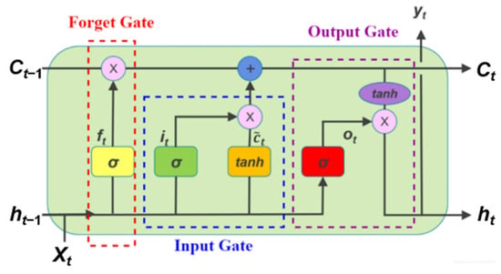
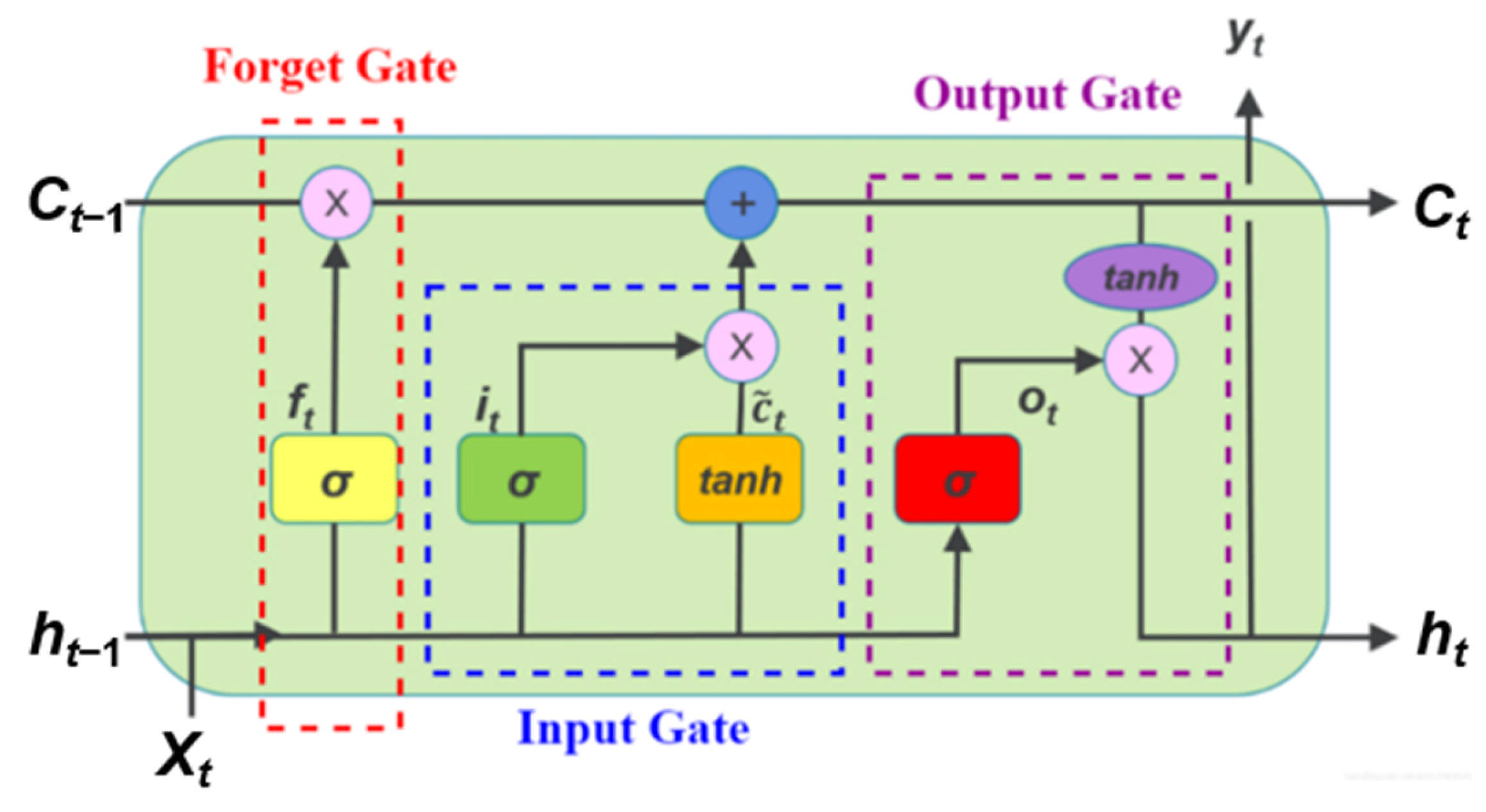
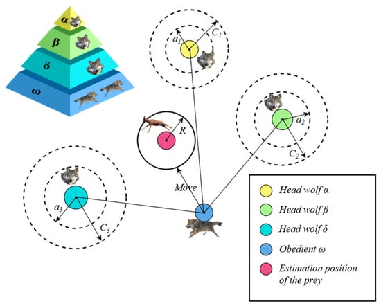
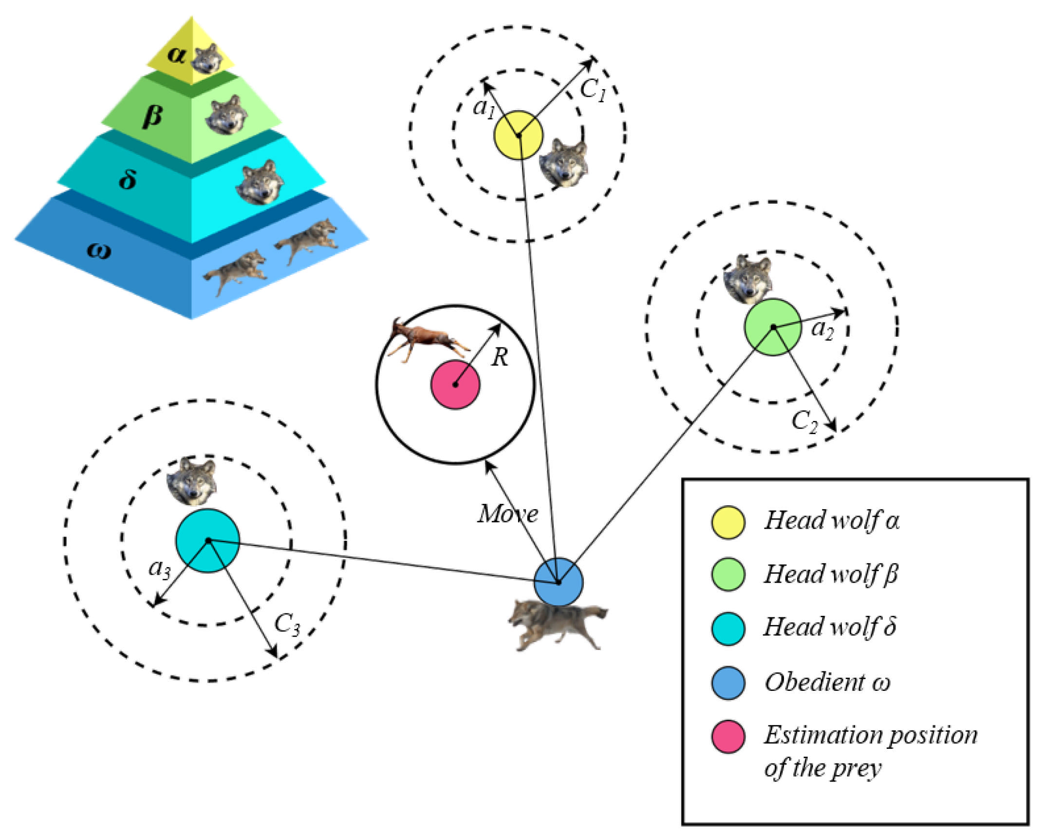
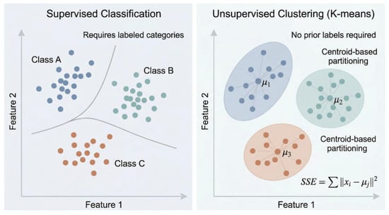
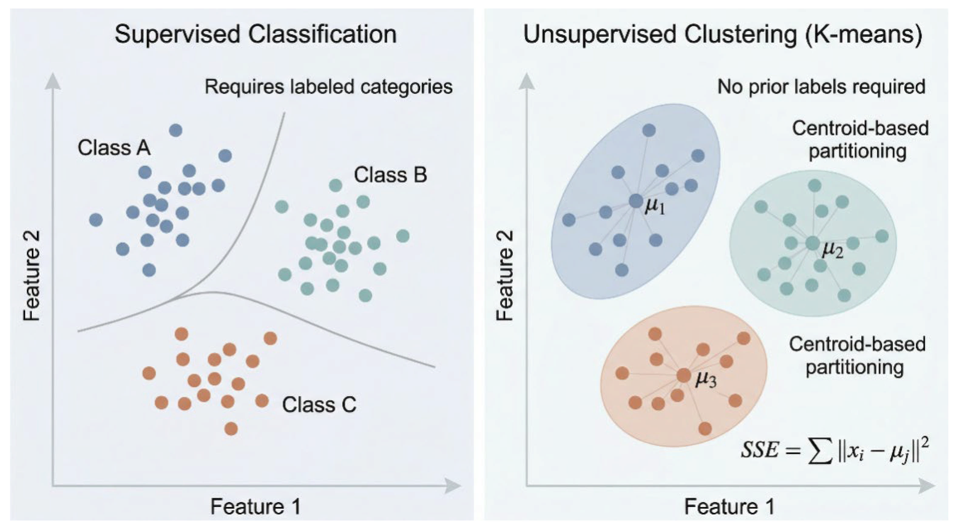
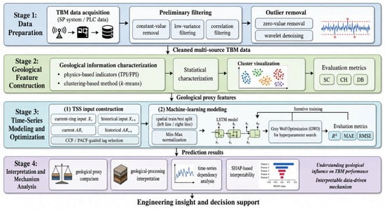
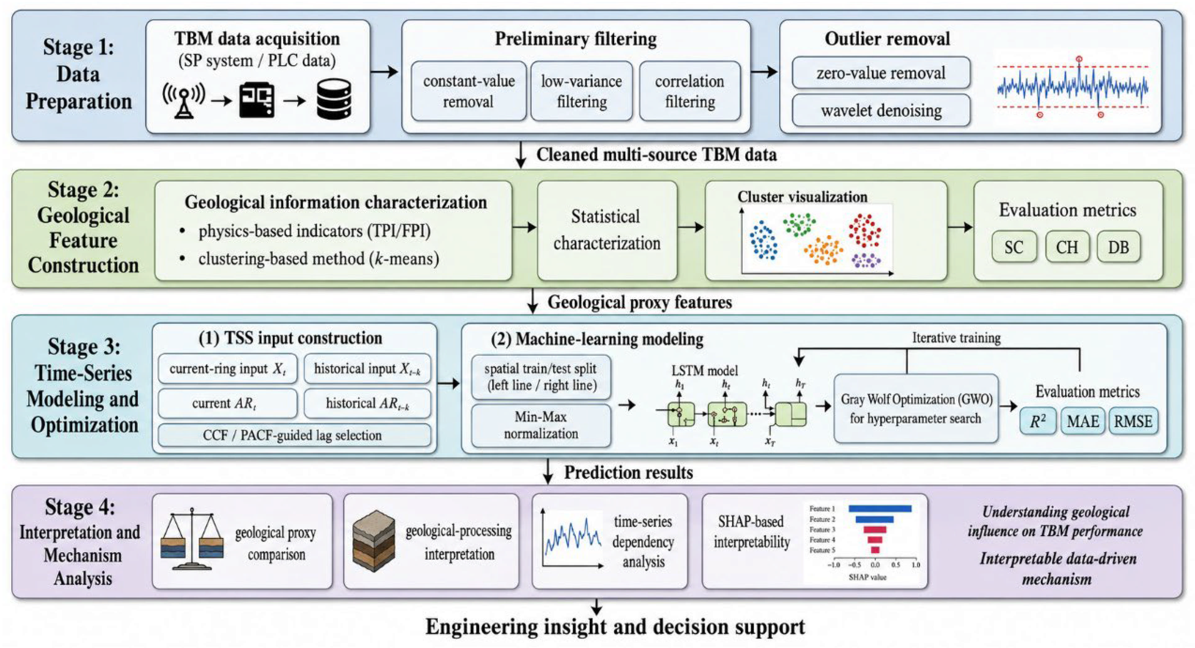
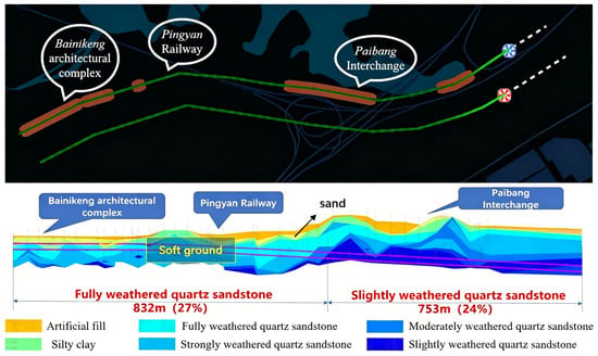
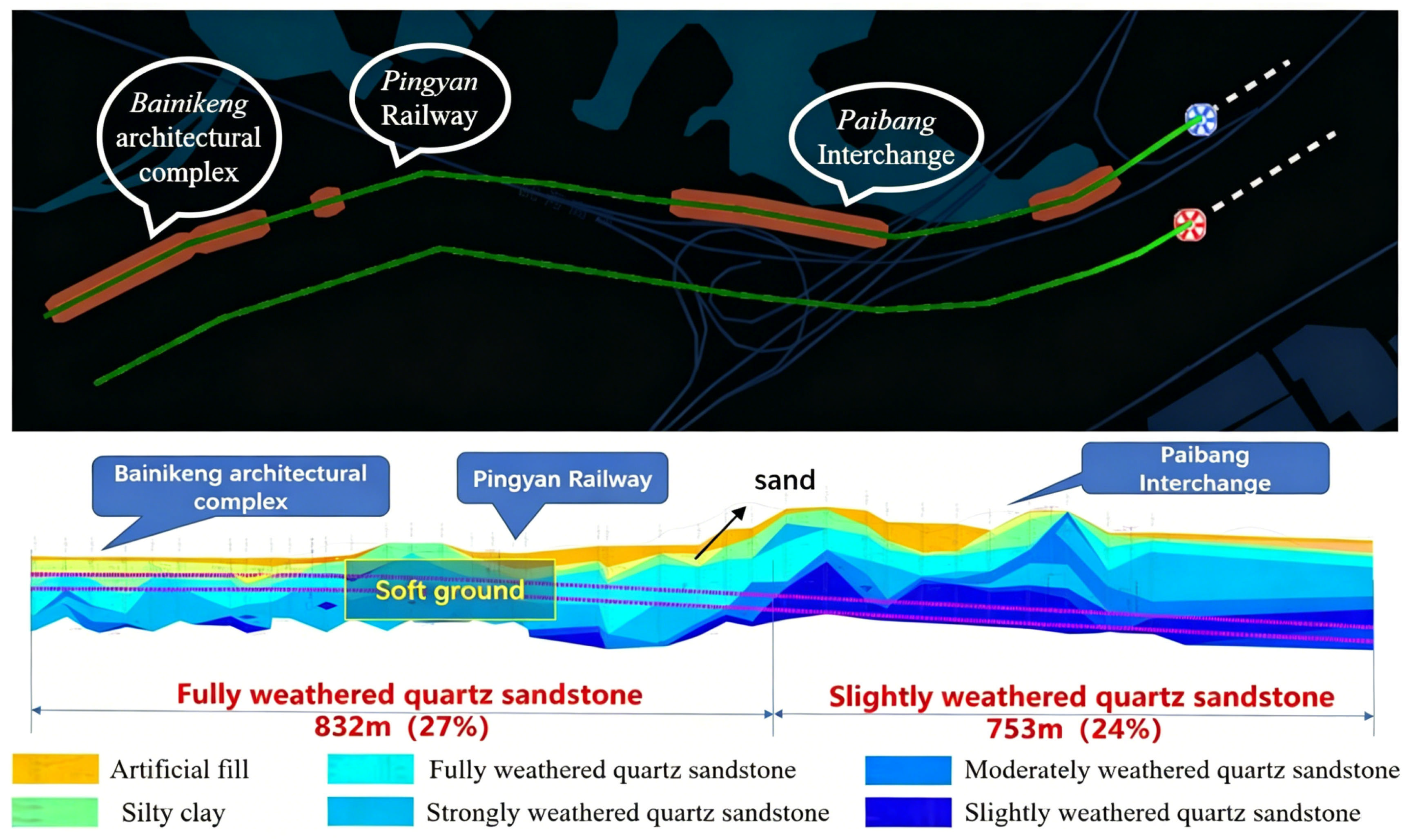
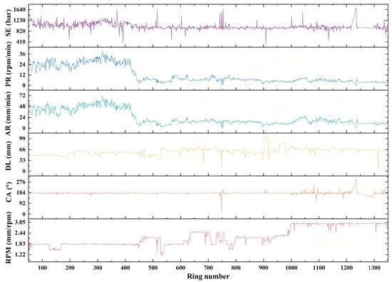
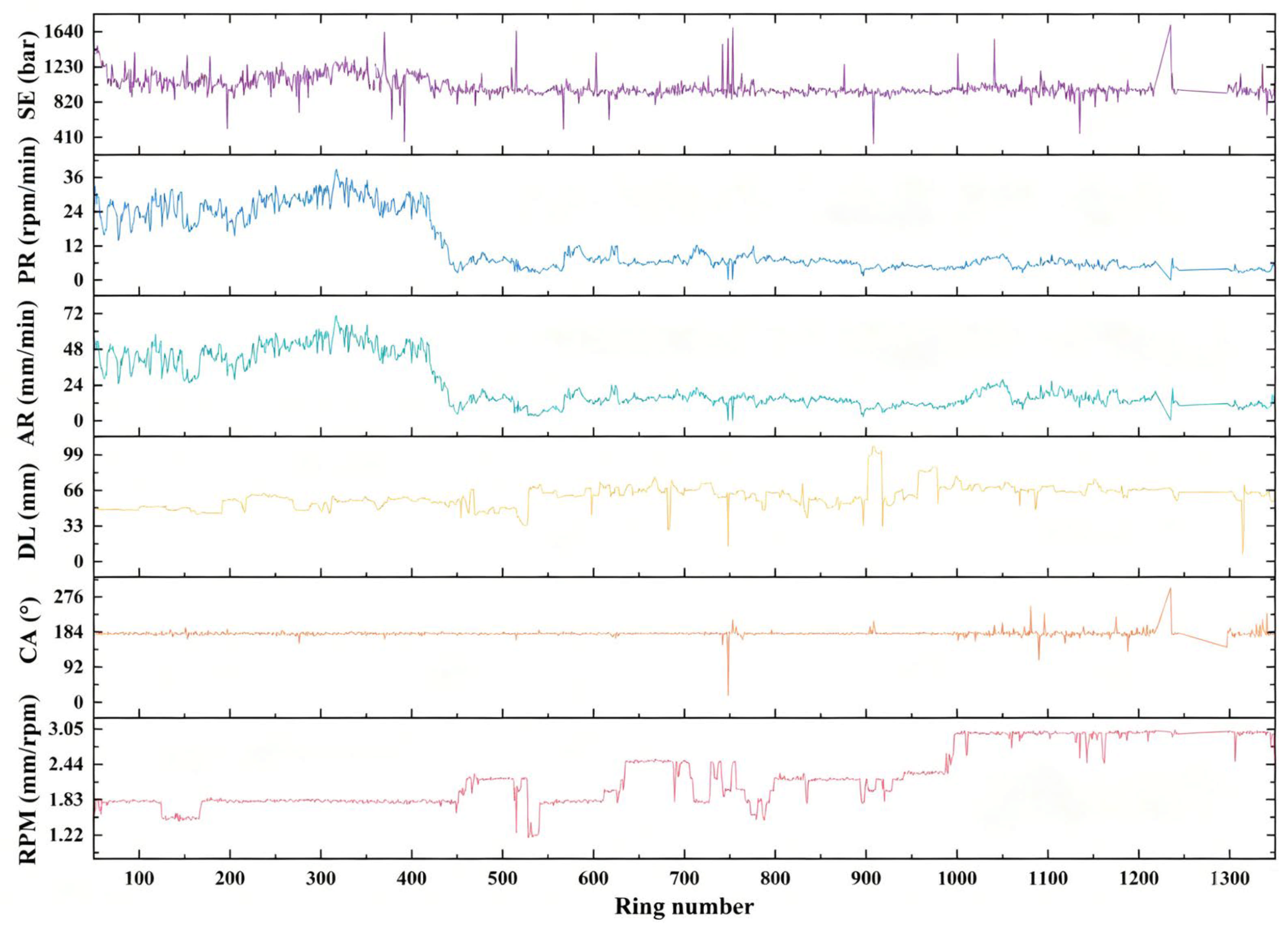
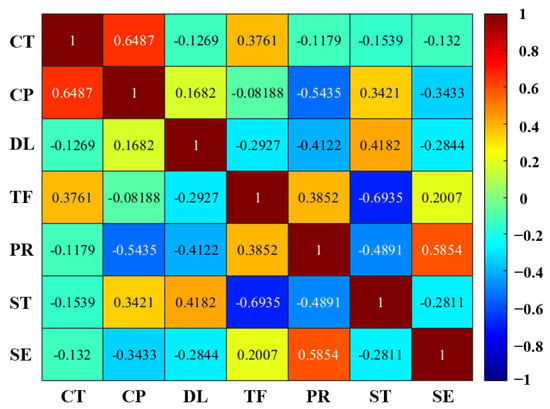
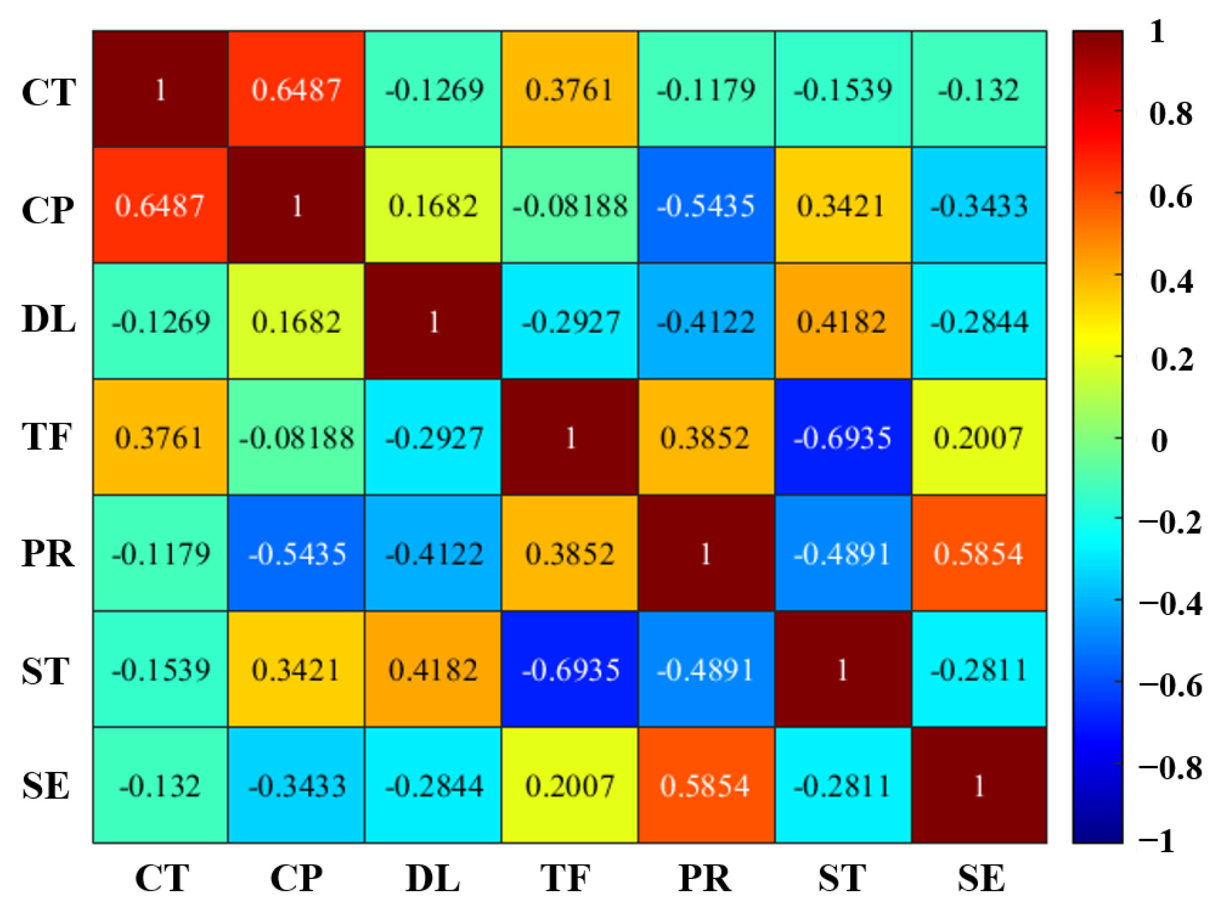
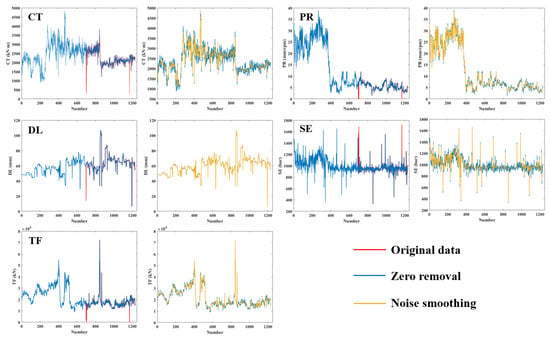
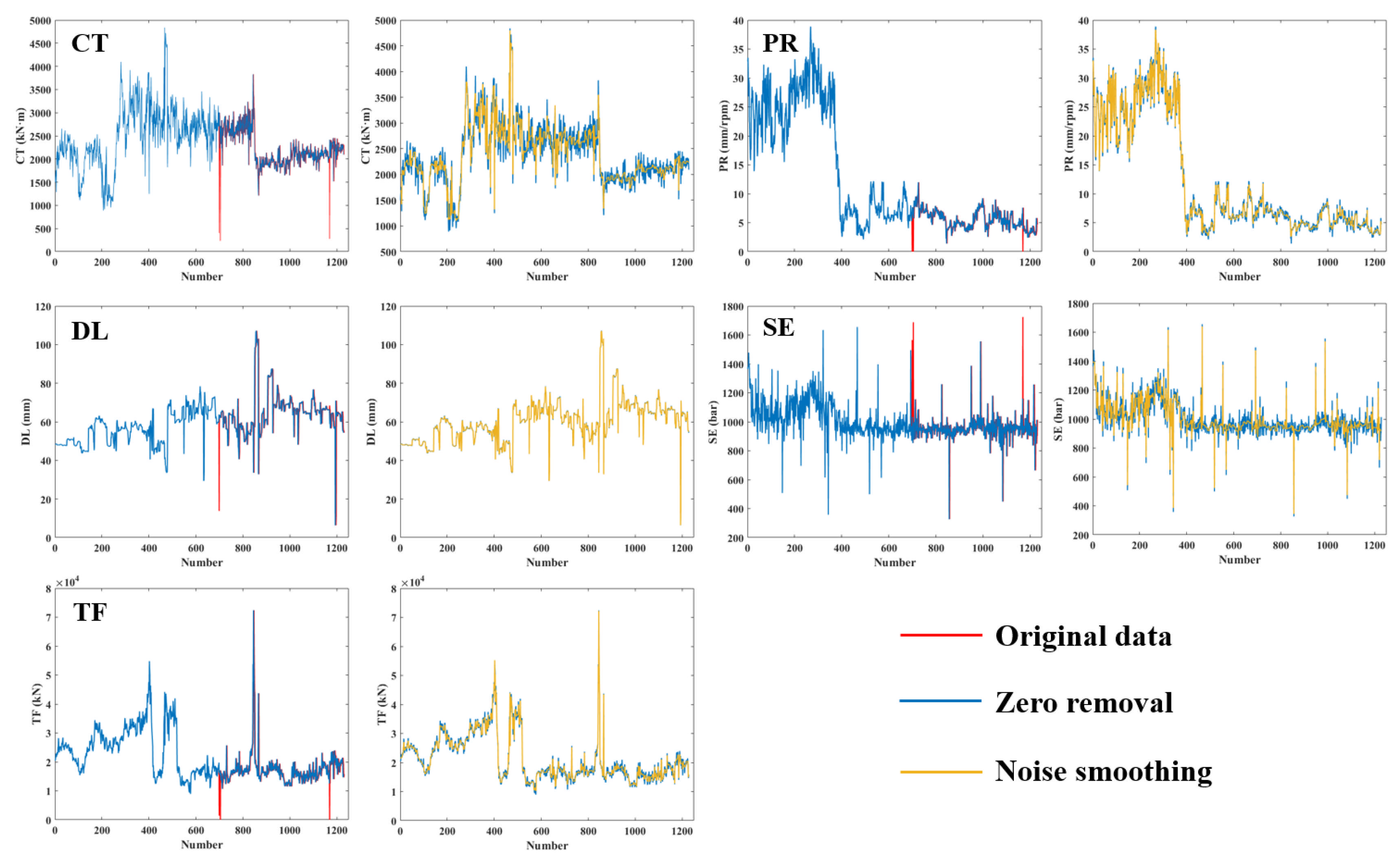
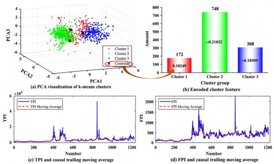
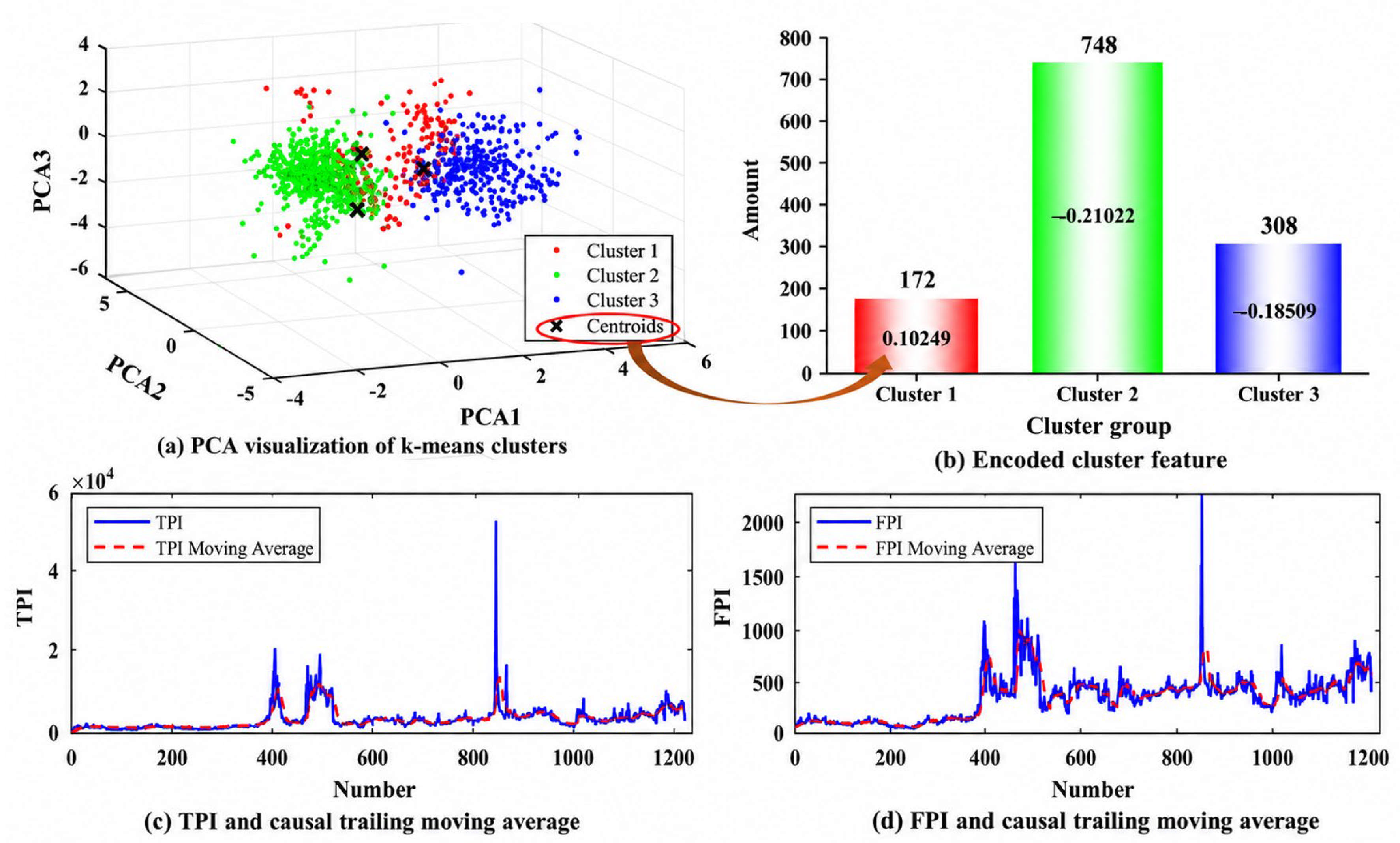
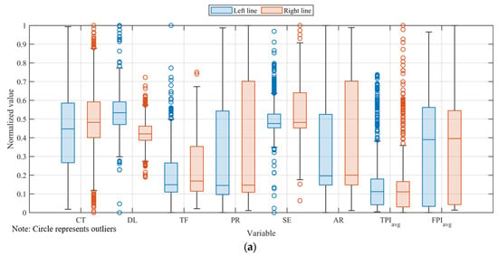
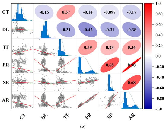
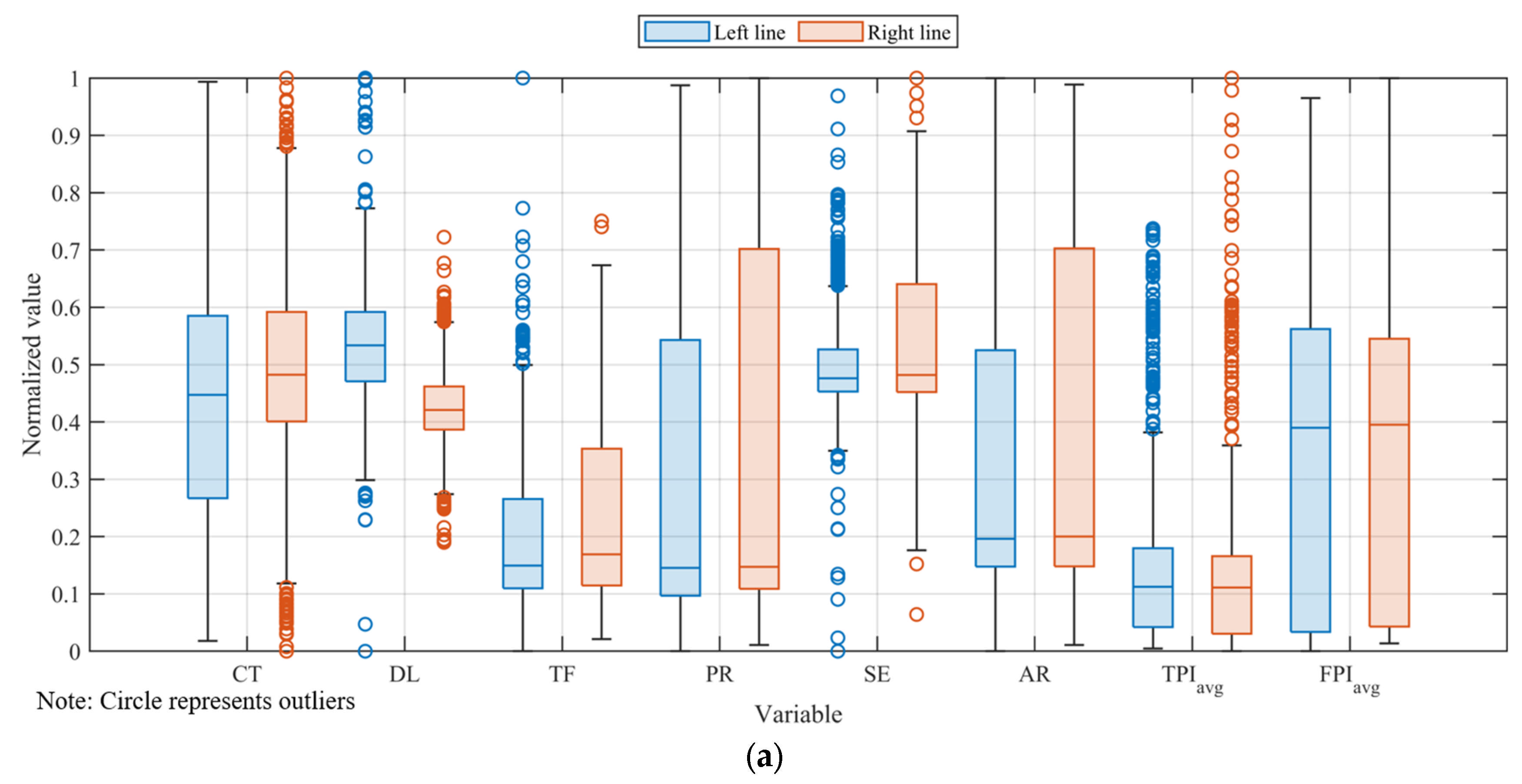
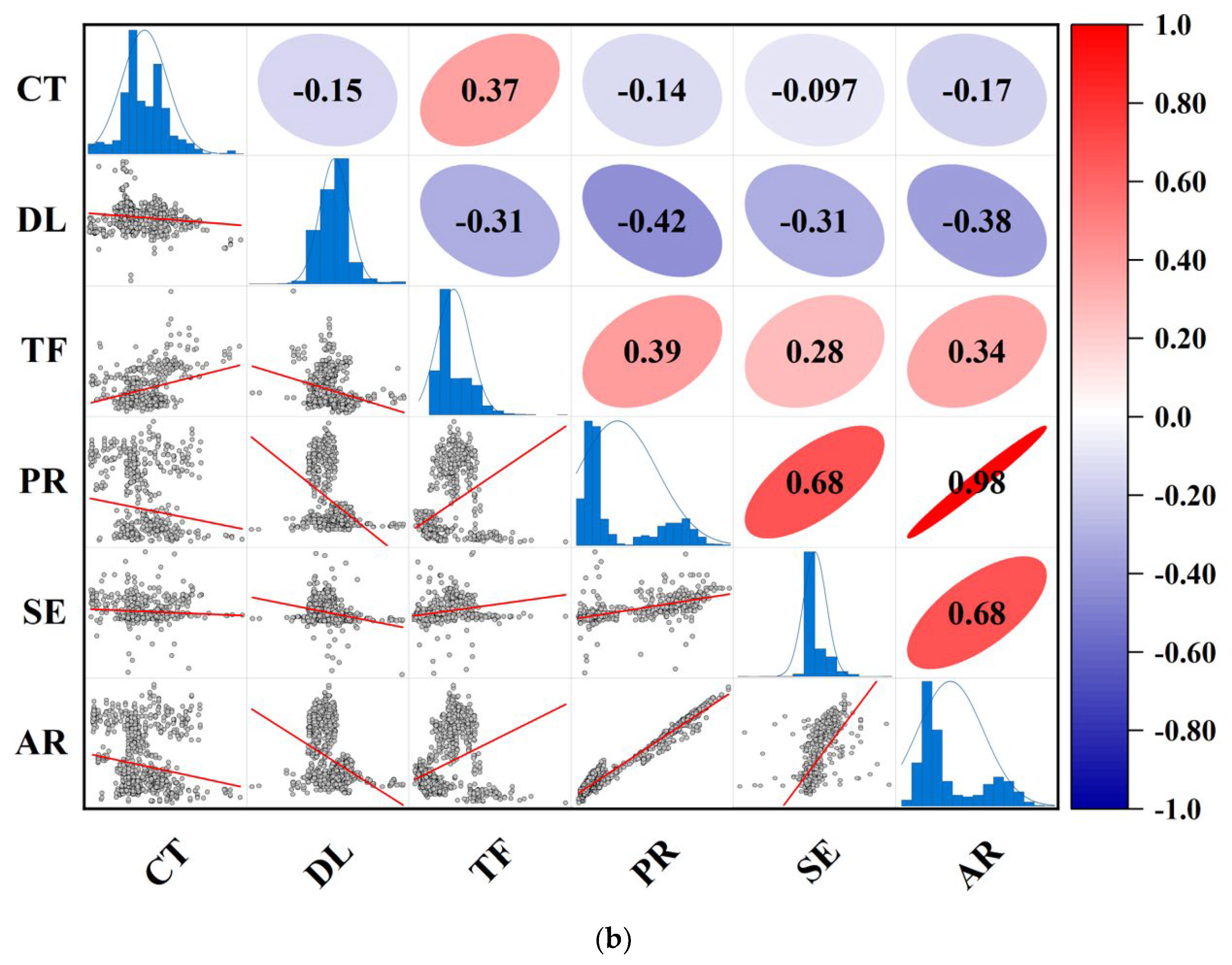
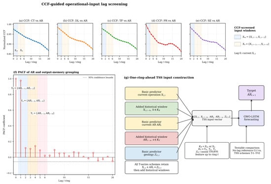
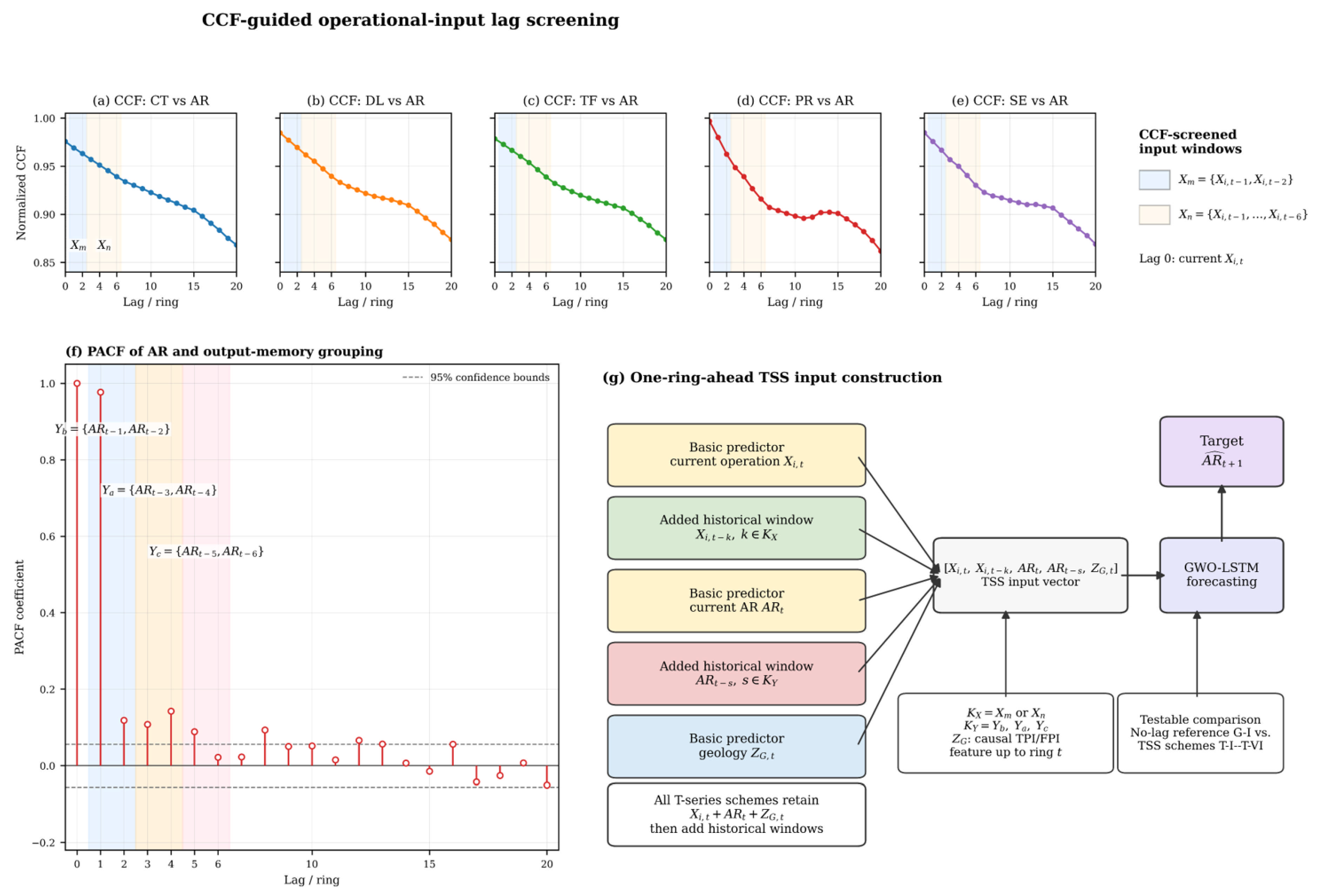
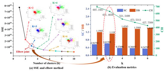
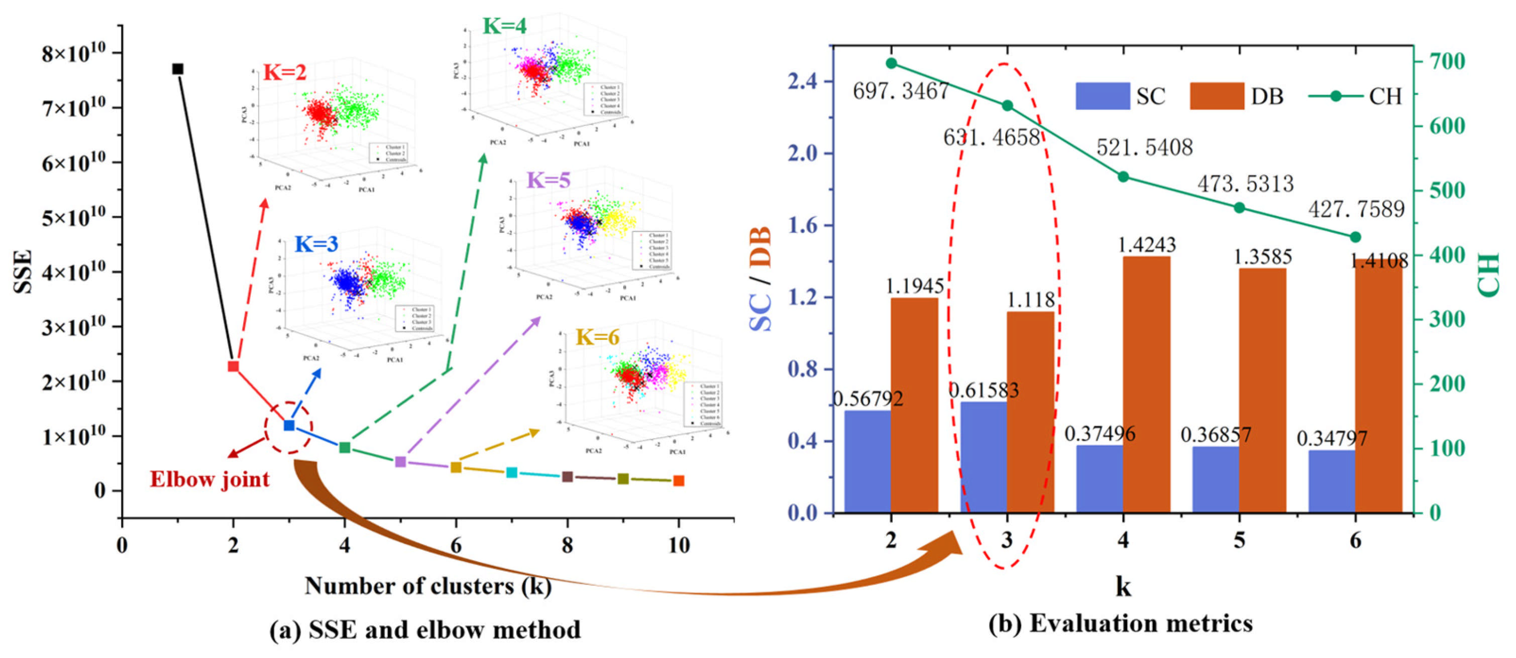
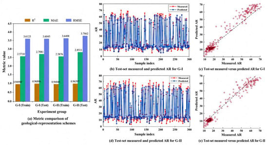
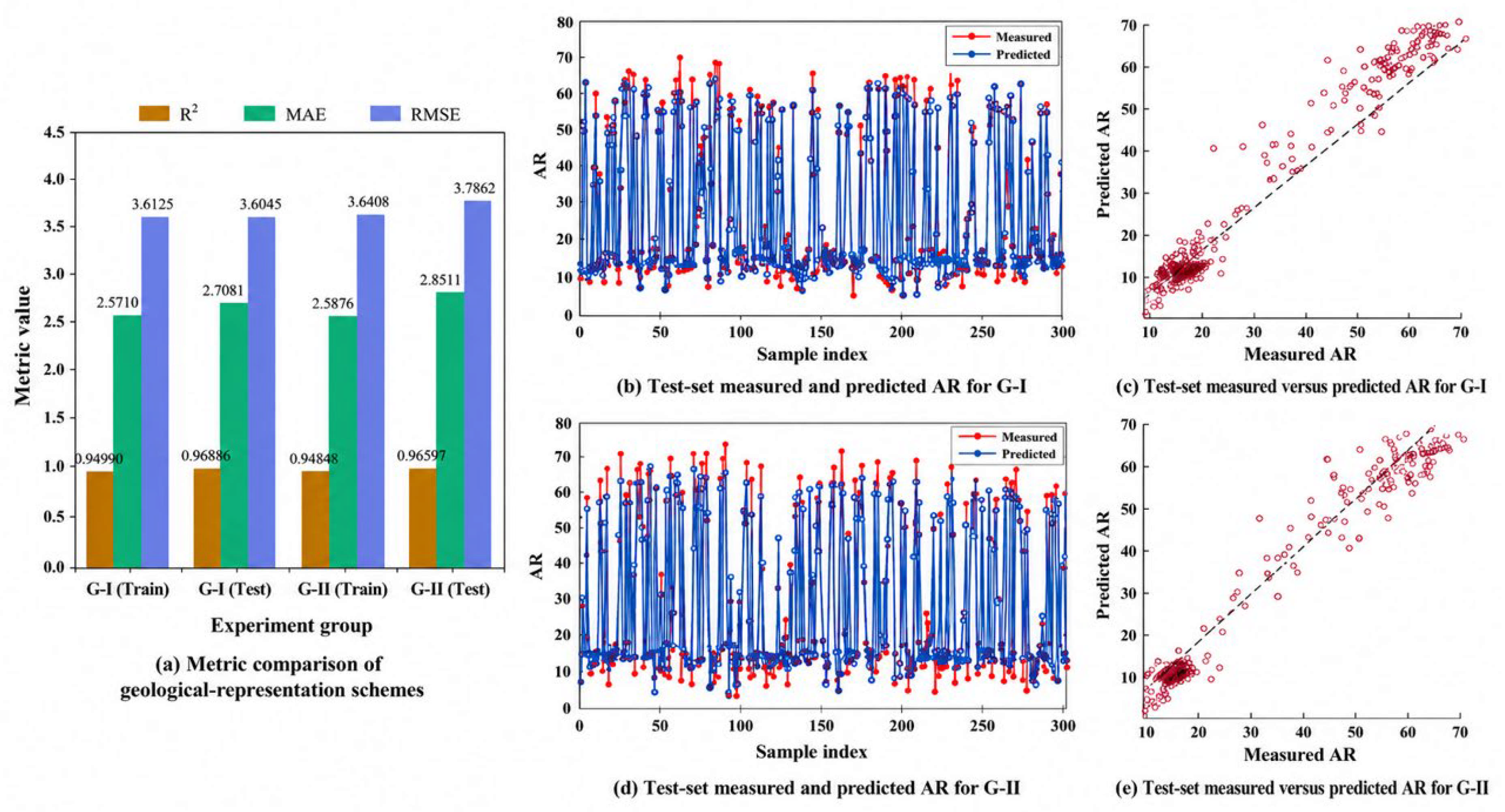
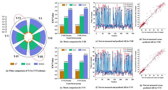
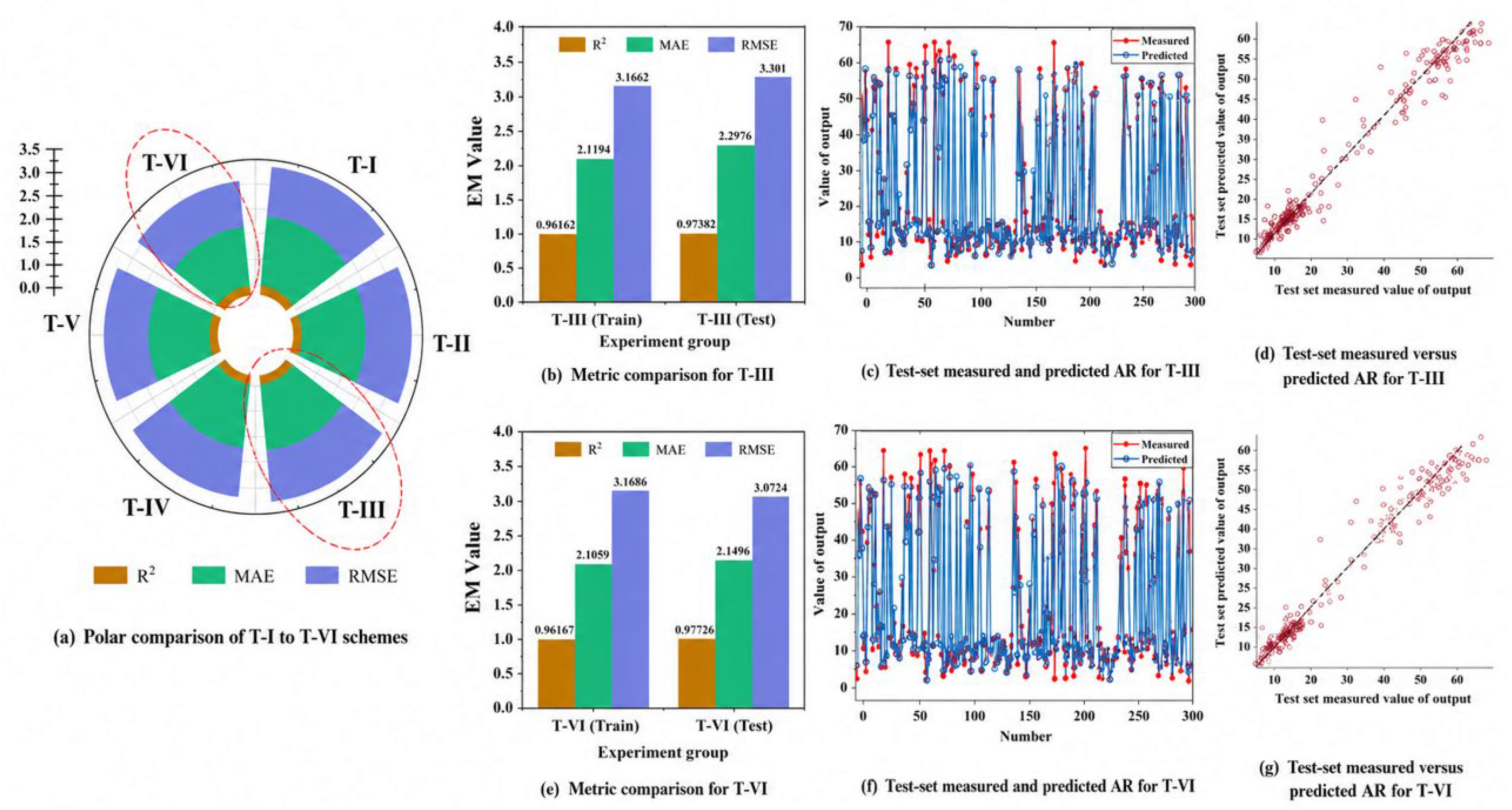
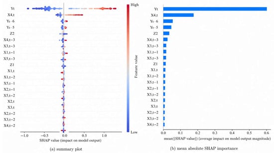
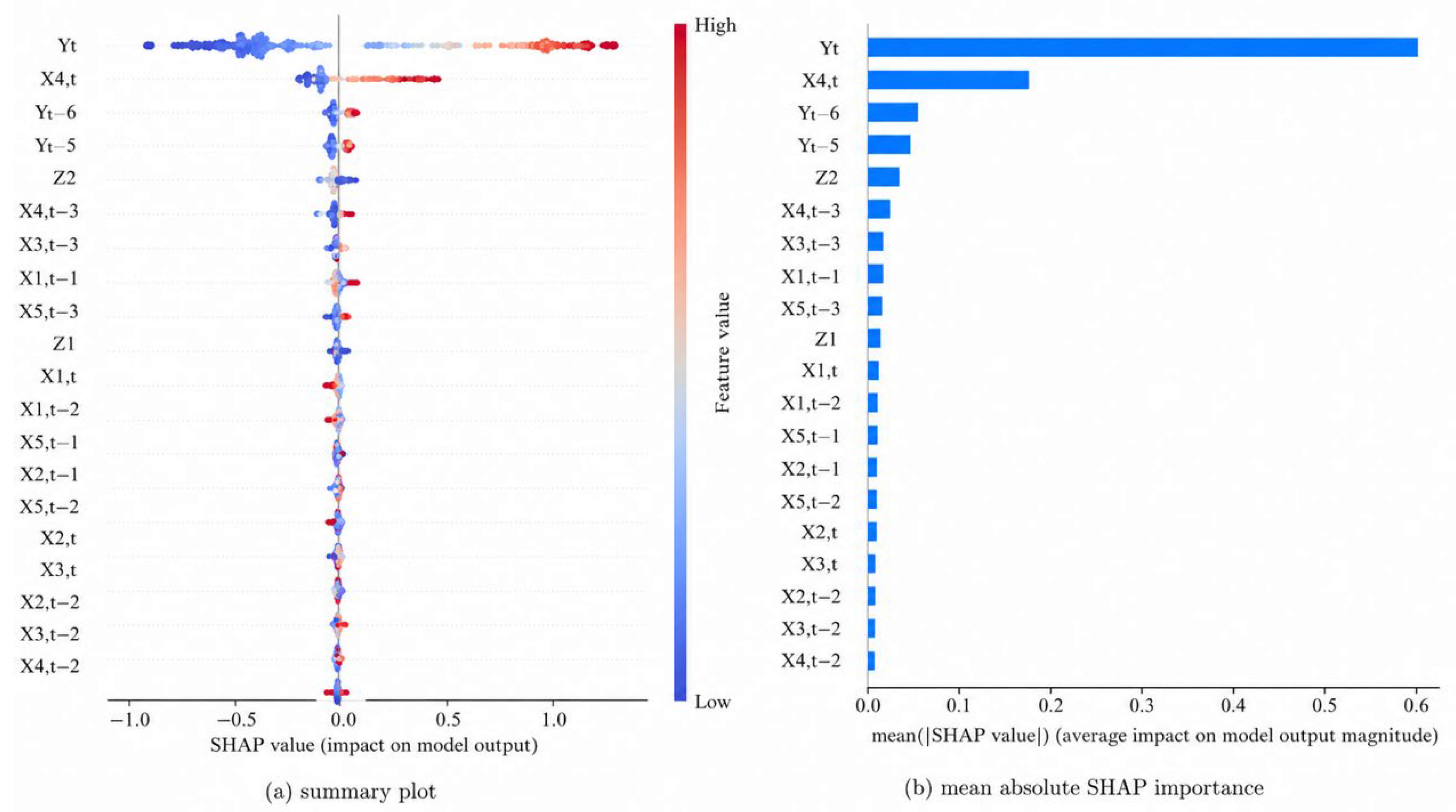

Disclaimer/Publisher’s Note: The statements, opinions and data contained in all publications are solely those of the individual author(s) and contributor(s) and not of MDPI and/or the editor(s). MDPI and/or the editor(s) disclaim responsibility for any injury to people or property resulting from any ideas, methods, instructions or products referred to in the content. |
© 2026 by the authors. Licensee MDPI, Basel, Switzerland. This article is an open access article distributed under the terms and conditions of the Creative Commons Attribution (CC BY) license.