Review

Physics-Informed Neural Networks in Aerospace Engineering: A Systematic Review of Architectures, Training Strategies, and Open Challenges


by
Przemysław Gryt
* and
Piotr Przystałka
Department of Fundamentals of Machinery Design, Faculty of Mechanical Engineering, Silesian University of Technology, 44-100 Gliwice, Poland
*
Author to whom correspondence should be addressed.
Appl. Sci. 2026, 16(13), 6282; https://doi.org/10.3390/app16136282
Submission received: 7 June 2026 / Revised: 18 June 2026 / Accepted: 19 June 2026 / Published: 23 June 2026

Abstract

This paper provides a systematic synthesis of recent developments in physics-informed neural networks (PINNs) applied to aerospace engineering, with an emphasis on their role in physically consistent surrogate modeling, forward simulation, and inverse parameter estimation. Using a PRISMA-based methodology, the study surveys peer-reviewed works published between 2017 and 2025 across aviation- and space-related domains, including aerodynamics, structural mechanics, aeroelasticity, propulsion, control, structural health monitoring, satellite-orbit prediction, space-debris collision avoidance, and spacecraft radiation-impact modeling. The analysis shows that embedding governing equations, boundary conditions, and observational data into composite loss functions enables PINNs to improve predictive consistency, reduce dependence on dense simulation or experimental datasets, and support parameter identification under sparse or noisy measurements. Attention is given to architectural variants such as XPINNs, cPINNs, gPINNs, operator-learning approaches, and hybrid PINN-CFD/FEM formulations, as well as to training strategies based on adaptive sampling, domain decomposition, transfer learning, and dynamic loss weighting. Reported benefits include reduced approximation error, improved convergence in selected high-gradient or multiphysics problems, and enhanced interpretability compared with purely data-driven models. At the same time, the review identifies persistent open challenges, including scalability to large aerospace domains, sensitivity to loss-weighting and collocation strategies, limited robustness under noise and uncertainty, high computational cost, and the lack of standardized aerospace benchmarks. Overall, the review highlights PINNs as a promising but still developing framework for fast, interpretable, and physically consistent modeling of aircraft and spacecraft systems.

1. Introduction

Physics-informed neural networks integrate deep learning architectures with governing physical laws, enabling the direct embedding of constraints imposed by partial differential equations (PDEs) into the training process [1]. They have emerged as an alternative framework for modeling systems governed by PDEs and other physical constraints, combining the interpretability of physics-based modeling with the adaptability of machine learning. This approach has demonstrated advantages across fluid mechanics, solid mechanics, and thermal processes [2]. In aviation and aerospace engineering, where aerodynamic modeling, structural dynamics, and structural health monitoring require capturing complex nonlinear behavior under varying load conditions, PINNs offer a promising alternative to traditional solvers by improving predictive accuracy while incorporating known physics into the model formulation. Their appeal is further strengthened by the growing demand for modeling turbulent aerodynamic flows, aeroelastic interactions, and multiphysics couplings where high-fidelity simulations typically incur prohibitive computational costs.
The modeling of such complex physical systems has traditionally relied on high-fidelity numerical solvers such as Computational Fluid Dynamics (CFD), the finite-element method (FEM), and coupled multiphysics frameworks. While these methods remain the foundation of modern aerospace analysis, they face well-known limitations: dense spatial discretization, extremely fine temporal stepping, high memory requirements, and poor scalability for turbulent, high Reynolds number, or strongly coupled problems. Moreover, many real-world aerospace tasks involve inverse formulations, where parameters must be inferred from sparse or noisy measurement scenarios in which classical solvers often require repeated forward simulations or heavy regularization. These constraints create a growing gap between the fidelity demanded by modern aerospace applications and the computational resources required to achieve it.
The emergence of scientific machine learning has introduced new opportunities to bridge this gap. Early neural network-based approximators exploited the universal approximation property to model physical systems. A major breakthrough came with the development of physics-informed neural networks, which embed governing equations directly into the loss function through automatic differentiation and residual minimization. The foundational work of Raissi, Perdikaris, and Karniadakis established PINNs as a general framework for solving forward and inverse problems governed by PDEs, enabling neural networks to satisfy conservation laws, boundary conditions, and constitutive relations during training. Subsequent advances, which include, e.g., XPINNs, gradient-enhanced PINNs, neural operators, and hybrid PINN–CFD/FEM formulations, have significantly expanded the applicability of physics-informed learning across scientific and engineering domains.
Aerospace engineering presents a uniquely demanding environment for such methods. Aerodynamic simulations frequently involve multiphysics coupling between fluid flow and structural deformation, and PINNs can incorporate these couplings without explicit meshing through meshless formulations [2]. By penalizing deviations from Navier–Stokes equations or structural elasticity formulations within the loss function, models can simultaneously predict flow fields and stress distributions. Comparative studies in turbulence modeling demonstrate that AI-augmented CFD frameworks integrating PINNs can achieve drag coefficient reductions and increased lift-to-drag ratios, outperforming baseline RANS and LES solvers. Additional quantitative improvements include reductions in mean squared error (MSE) of up to 85% when domain decomposition strategies are applied to high-Reynolds-number flows [3]. Domain decomposition further enables localized training on smaller subproblems, improving scalability for large aerodynamic simulations.
The effectiveness of PINNs depends strongly on the choice of loss functions and training strategies. Weighted residual losses that combine physics-based terms with data-fitting components improve convergence stability, particularly for high-frequency oscillatory phenomena relevant to aeroacoustics modeling [4]. Hard enforcement of boundary conditions, such as exact Dirichlet constraints on wing surface pressure, has been shown to produce more physically consistent results compared to soft penalty approaches [3]. Architectures such as dual-network PINNs enable separation of forward prediction and inverse parameter estimation tasks, which is particularly useful in structural health monitoring applications. Advanced turbulence models embed physics-informed residual terms derived from Navier–Stokes equations directly into the loss function, enabling adaptive optimization strategies such as particle swarm tuning [4,5]. Adaptive sampling strategies that concentrate collocation points in regions with steep gradients can reduce loss values by up to 50% compared to uniform sampling.
Architectural variations also play a crucial role in performance. Fourier Neural Operators (FNOs) and DeepONets provide improved accuracy in multiscale problems but often require substantial computational resources [1,5]. Hybrid PINN–CFD approaches offer a compromise between accuracy and efficiency, while coupling with finite-element methods or domain decomposition enhances scalability for large domains, albeit at the cost of increased implementation complexity. Interpretability remains an important advantage of PINNs: sparse architectures combined with symbolic rule extraction enable tracing of how parameters such as angle of attack or control surface deflection influence lift coefficients [6].
Despite these advantages, several challenges remain. Scalability continues to limit large domain applications, particularly in cases involving dense multiphysics coupling [2]. Handling noisy or sparse sensor data also presents difficulties; approaches such as Lasso PINNs improve robustness but require careful tuning of regularization parameters. The absence of standardized benchmark datasets and evaluation protocols complicates comparisons across studies and reduces reproducibility. Practical deployment in aerospace systems requires integration with high-performance computing platforms [6]. Beyond aerodynamics, PINNs are increasingly applied in related aerospace subsystems, such as grid-connected inverter control, where they support parameter estimation and fault detection under uncertain operating conditions [7].
Although the body of literature on physics-informed neural networks has grown rapidly in recent years, research relevant to aerospace engineering remains distributed across multiple disciplinary domains. Valuable contributions exist in fluid mechanics, structural mechanics, structural health monitoring, propulsion, control theory, and scientific computing; however, these studies are typically developed within their respective communities, with limited cross-domain integration. As a result, the field lacks a consolidated synthesis that organizes existing approaches, clarifies methodological commonalities, and highlights how solution strategies developed for one class of governing equations can be transferred to others that are frequently encountered in aerospace applications.
This review is motivated by the need for integration rather than by any absence of prior work. Its goal is to provide a coherent, application-oriented overview of PINN architectures, training strategies, physical formulations, and computational techniques used across aerospace-related problems.
Beyond synthesizing the state of the art, this review addresses a broader research question concerning the practical suitability of physics-informed neural networks for modeling aircraft dynamics. The authors investigate whether PINN-based surrogate models can provide a fast, interpretable, and physically consistent representation of aircraft motion while preserving the key constraints imposed by flight mechanics. This question is particularly relevant for model-based optimization tasks, where repeated simulations of aircraft behavior are required, for example, in mission planning, trajectory optimization, or control-oriented analysis. By mapping existing PINN architectures, training strategies, physical formulations, and application domains, the review identifies transferable methodological patterns that may support the development of next-generation surrogate models for aerospace dynamics. In this context, the article provides not only a synthesis of current knowledge but also a foundation for assessing the feasibility of using PINNs as computationally efficient models in optimization and decision-support workflows. Unlike existing general reviews of physics-informed neural networks, this article adopts an explicitly aerospace-oriented perspective. Rather than surveying PINN methodology in a domain-agnostic manner, the review focuses on how specific architectures, training strategies, and physical formulations translate to aerodynamic modeling, structural dynamics, aeroelasticity, propulsion, spacecraft environments, and flight-dynamics problems. The discussion emphasizes methodological patterns that are transferable across these aerospace subdomains and highlights challenges that are unique to high-fidelity aerospace simulations, such as multiphysics coupling, high-Reynolds-number flows, sparse sensor environments, and the absence of standardized aerospace benchmarks. This domain-specific framing distinguishes the present review from broader PINN surveys and positions it as a targeted synthesis for aerospace researchers and practitioners.

2. Review Methodology

This review was conducted in accordance with the principles of systematic literature analysis and the PRISMA guidelines (Figure 1), with specific consideration of research on physics-informed neural networks in aerospace engineering. The objective of the methodology was to ensure a transparent, reproducible, and auditable procedure for selecting publications covering both the theoretical foundations of PINNs and their applications in aerodynamics, structural mechanics, propulsion, control systems, and diagnostics.
The literature search was performed in three major scientific databases: Scopus, Web of Science (WoS), and IEEE Xplore, covering publications from 2017 to 2025, corresponding to the period of rapid development of PINN-based methods and their variants. The search was limited to peer-reviewed journal articles and conference papers in engineering, computational science, and machine learning.
To improve transparency and reproducibility, the exact search strings and screening workflow are detailed here. The database queries combined PINN-related terms with aerospace-domain terms using Boolean operators. A representative search string was: (“physics-informed neural network” OR “PINN” OR “XPINN” OR “gPINN” OR “operator learning” OR “scientific machine learning”) AND (“aerospace” OR “aerodynamics” OR “flight dynamics” OR “aeroelasticity” OR “structural health monitoring” OR “propulsion” OR “spacecraft”). The initial search returned 312 records from Scopus, 284 from Web of Science, and 167 from IEEE Xplore. After automatic and manual duplicate removal, 421 unique records remained. Title- and abstract-level screening excluded studies unrelated to PINNs or unrelated to aerospace applications, resulting in 146 papers for full-text assessment.

2.1. Search Strategy

The search strategy was based on two groups of keywords: terms related to PINNs and physics-informed machine learning and terms related to aerospace engineering and its subdomains.
Within each group, the OR operator was used to capture terminological variations across the literature.

2.2. Study Selection

All records matching the search criteria were retrieved from Scopus, WoS, and IEEE Xplore:
  • Duplicate entries were removed automatically;
  • Remaining duplicates were removed manually.
Publications that passed the screening stage were evaluated in full to determine whether they met the inclusion criteria.

2.3. Inclusion and Exclusion Criteria

A publication was included if it met all the following conditions:
  • It applied PINNs or related physics-informed methods (XPINN, gPINN, operator learning, or hybrid PINN CFD/FEM).
  • It addressed a problem within aerospace engineering (aerodynamics, structures, SHM, propulsion, control, or space systems).
  • It presented quantitative results, methodological analysis, or comparison with classical numerical methods.
  • It was published in a peer-reviewed venue.
Publications were excluded if they:
  • Were unrelated to PINNs or unrelated to aerospace;
  • Were purely theoretical without engineering relevance;
  • Were not peer-reviewed;
  • Duplicated content from other works by the same authors.

2.4. PRISMA Flow Description

The selection process followed the following PRISMA logic:
  • Records identified in Scopus, WoS, and IEEE Xplore.
  • Duplicates removed automatically and manually.
  • Records screened based on titles, keywords, and abstracts.
  • Records excluded due to lack of relevance to PINNs or aerospace.
  • Full-text articles assessed for eligibility.
  • Final set of publications included in the review.

2.5. Extracted Factors

From each publication, the following information was extracted:
  • Problem type (forward/inverse, PDE class).
  • Architecture used (PINN, XPINN, FNO, DeepONet, or hybrid).
  • Loss function structure (residuals, BC/IC, data fit, and weighting).
  • Training strategy (adaptive sampling, domain decomposition, and gradient normalization).
  • Evaluation metrics (MSE, L2 error, boundary residuals, and convergence rate).
  • Aerospace application domain (aerodynamics, structures, SHM, propulsion, and control).

3. Fundamentals of Physics-Informed Neural Networks

3.1. Conceptual Foundations

Embedding physical laws directly into neural network architecture changes the learning process from purely statistical approximation into constrained optimization within a physically admissible solution space. In physics-informed neural networks, this is achieved by incorporating governing equations such as Navier–Stokes equations, elasticity theory, Maxwell’s equations, or other conservation principles directly into the loss function or, in some cases, into the network architecture itself. The formulation penalizes deviations from these laws alongside traditional data-fitting errors, leading to solutions that comply with both measured observables and theoretical constraints [4,6]. In practical terms, this means that the governing equations of a given physical system, whether in the form of partial differential equations (PDEs), ordinary differential equations (ODEs), or conservation principles, are embedded directly into either the structure or optimization objective of the neural network [6,8].
For aviation and aerospace applications, such integration is particularly important because it enables models to handle multiphysics scenarios such as coupled fluid–structure interactions without relying solely on dense and often unobtainable experimental datasets. These constraints may include Navier–Stokes equations for turbulent aerodynamic flows, continuity laws for mass conservation, or turbulence transport equations applicable to Reynolds-Averaged Navier–Stokes (RANS) and Large Eddy Simulation (LES) contexts [8,9]. The embedding process typically involves adding residual minimization terms alongside traditional data-fitting losses, and the resulting models are then validated against high-fidelity numerical solutions to ensure no violation of physical consistency. In aerospace settings, this may involve comparing predicted velocity fields, pressure distributions, or displacement profiles against CFD solutions or structural simulations.
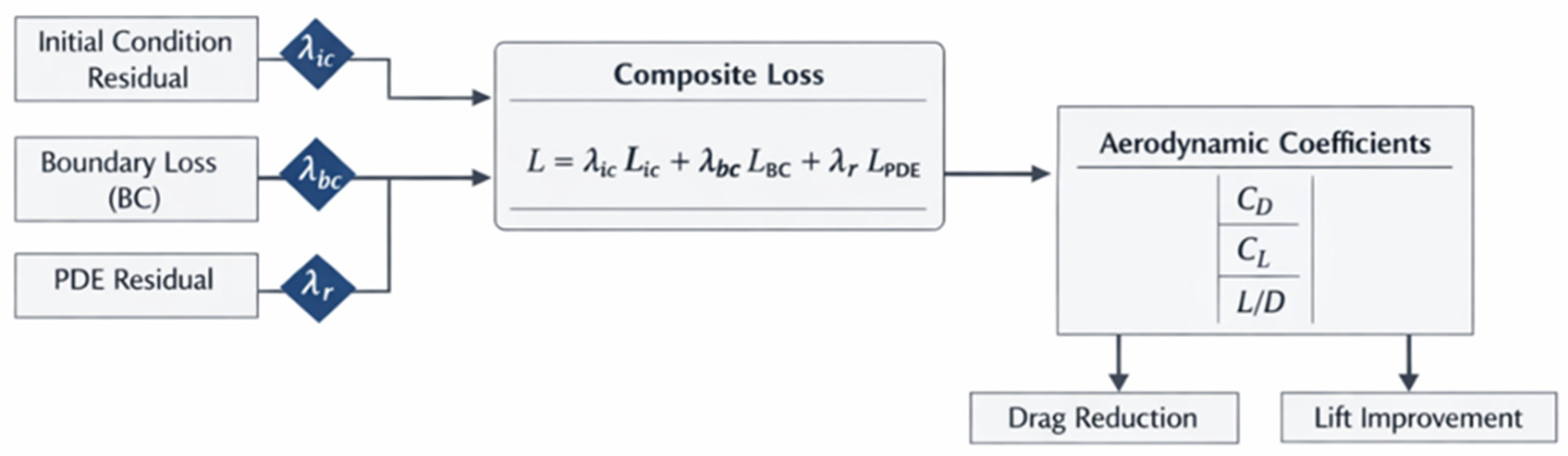
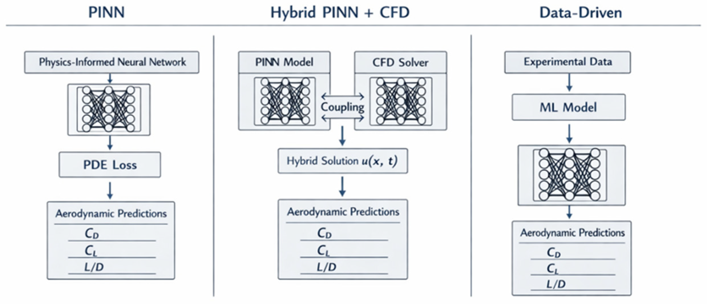
A representative composite loss for turbulence modeling can be formulated so that λ i c , λ b c , and λ r control the weighting between initial conditions, boundary conditions, and residual PDE enforcement. In aerospace applications, this allows networks to predict velocity fields and pressure distributions over aerodynamic surfaces while maintaining fidelity to conservation laws of mass and momentum. For example, hybrid PINN + CFD implementations embedding Navier–Stokes residuals have reported reductions in drag coefficient from C d = 0.03 to C d = 0.018 together with lift-to-drag increases of 50%, outperforming baseline RANS solvers under identical mesh configurations [8]. Empirical studies more broadly show that PINNs can achieve accuracy levels comparable to established numerical approaches while using much smaller datasets [7]. For aerodynamic modeling over aircraft wings, feedforward PINNs trained with synthetic CFD data have been shown to match computed lift coefficients while capturing wake structures with error margins comparable to mesh-based solvers.
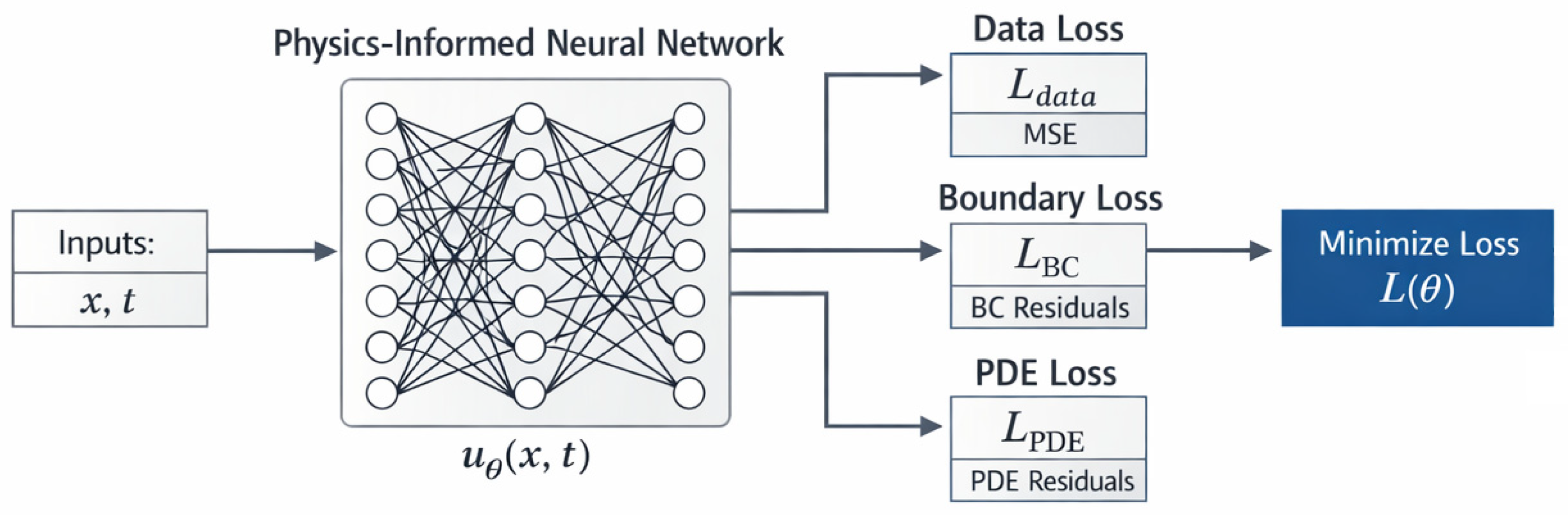
The diagram presents a standard PINN architecture (Figure 2) in which the neural network u θ ( x , t ) receives spatial–temporal inputs and minimizes a composite loss function combining data misfits, boundary-condition residuals, and PDE residuals. This multi-component formulation enforces physical consistency during training, enabling the model to recover solutions that satisfy both measurements and governing equations.
One critical observation from recent studies is that enforcing physical constraints not only improves accuracy but also reduces dependency on large and labeled datasets. By replacing part of the empirical loss with physics-based terms, required training samples often decrease substantially. For instance, PINN frameworks for laminated composite bending behavior have been validated against finite-element results using less than 10% of the data required by purely data-driven models [10]. In grid-connected inverter control tasks relevant to aircraft electrical subsystems, PINNs leveraging embedded Kirchhoff’s laws reconstructed hidden states from sparse voltage/current measurements without supervised trajectories. Similarly, graph-based PINNs (GNN-PINNs) for power-grid state estimation achieved over 20% lower MSE than conventional estimators, though at the cost of extensive optimization of composite losses [7].
Another important factor is interpretability. Embedding known physics allows engineers to trace the influence of specific variables on outputs. For example, one can identify how changes in angle of attack affect lift gradient predictions within the network’s learned mapping [6]. Studies on laminated composites further illustrate how domain-specific physical laws can be embedded at different levels: some formulations integrate Classical Laminated Plate Theory directly into the loss, whereas hybrid architectures incorporate Sublaminate Generalized Unified Formulation with Extreme Learning Machine optimizers to address complex geometries beyond clamped plates. Explicit enforcement of equilibrium and compatibility conditions ensures that predicted stress and strain fields remain consistent with material mechanics principles even under extrapolative scenarios.
Extraordinary variants include spectral-domain approaches such as k-space PINNs embedding Fourier-based mappings within physical residuals to capture vibrational modes efficiently. These methods have reduced mode-shape prediction errors down to 1.44 × 10 − 3 , outperforming time-domain formulations in composite vibration analysis. Disjoint subnetworks form another direction: splitting temperature evolution and degree-of-cure PDEs into separate modules has maintained accuracy below 10 − 5 loss values in autoclave curing simulations while accommodating sharp interface discontinuities [10].
The diagram presented in Figure 3 illustrates the individual loss components: initial condition residuals, boundary-condition errors, and PDE residuals. Those are combined into a weighted composite loss function. By tuning the weighting factors λ i c , λ b c , and λ r , the optimization process can emphasize different physical constraints during training. The resulting composite loss directly affects the predicted aerodynamic coefficients C D , C L , and L / D , enabling targeted improvements in drag reduction and lift enhancement.
However, integrating physical constraints also introduces significant challenges. High-dimensional PDEs lead to stiff residual landscapes that complicate convergence, especially when multiscale processes are modeled simultaneously, such as high-Mach compressible flow coupled with aeroelastic deformation. Large neural networks may be needed to capture these dynamics accurately, driving up training costs and memory requirements. Training PINNs embedded with complex multiphysics laws can extend computational times significantly due to residual evaluation at each collocation point across potentially high-dimensional domains. For large-scale simulations common in aerospace, such as full-airframe turbulent wake prediction, the cost of residual computation can rival that of direct CFD unless efficiency optimizations like reduced-order modeling or adaptive sampling are employed [2].
Moreover, there is a sensitivity to hyperparameter tuning, particularly weighting coefficients between physics-based terms and empirical data terms. Imbalanced weights can lead either to physically plausible but numerically inaccurate outputs or to overly data-fit solutions that violate conservation laws. Adaptive weighting strategies can halve total loss values compared with fixed weights when balancing collocation-point residuals against boundary-condition penalties in shock-dominated flows. Yet poorly tuned weights may destabilize training or underfit specific regions of the state space, and unresolved questions remain regarding how to automate this tuning across diverse aerospace regimes. Experimental comparisons further indicate that while PINNs can reduce manual effort relative to solver-based baselines such as FEM/SLSQP, they may struggle in noisy inverse problems when the physics-loss term inflates uncontrollably, particularly under adaptive weighting schemes where gradients become imbalanced between data-driven and residual components [11].
Aerospace-specific implementations also reveal gaps in benchmark availability. While areas such as climate modeling and structural mechanics already provide shared datasets for PINN evaluation, aviation lacks widely accepted benchmark tasks against which methods can be objectively tested [12]. Without standardized reference problems spanning aerodynamic surfaces under both laminar transition and turbulent separation, along with electrical system faults during flight cycles, reported loss values across studies must be interpreted cautiously. Differences often reflect not only architectural choices but also variations in setup, geometry, noise level, and preprocessing. This lack of standardization makes it challenging to determine whether methodological differences genuinely improve generalization or merely suit a specific simulation configuration.
Notably, hybrid approaches that incorporate both physics-informed operators and probabilistic uncertainty quantification are gaining traction [13]. These combinations may prove useful for aerospace engineering, where environmental variability and noise measurement are inherent. For example, combining dropout-based epistemic uncertainty with embedded PDE constraints could better inform flight-control systems adjusting to rapid weather changes. A parallel may be drawn between aerospace fluid dynamics and power electronics for aircraft systems: both require preserving stability margins under dynamic loading while predicting unmeasured states from limited empirical input. Methods combining Lyapunov-based stability certification with physics-informed losses have demonstrated resilience against parameter uncertainty in microgrid simulations for avionics systems, retaining transient stability despite topology changes [7].
Table 1 contrasts a range of PINN architectures and deep learning surrogates evaluated on canonical benchmarks, including RANS flows, stiff PDEs, composite mechanics, and nonlinear reaction–diffusion systems. The results demonstrate that architectural depth, loss balancing strategies, and numerical enhancements have a decisive impact on accuracy and convergence. Notably, several specialized variants outperform baseline PINNs by large margins, underscoring the importance of tailored training pipelines for challenging physical regimes.
Interestingly, studies outside aerospace contexts have reported a similar tension between computational effort and model generalization when governing PDE terms are enforced via weighted MSE components alongside displacement or force boundary conditions; such formulations may achieve impressive fit quality yet remain sensitive to noisy inputs unless weights are adaptively balanced [16]. This cross-domain observation suggests that stronger theoretical adherence through multi-term physics losses may require dedicated balancing mechanisms if performance gains are to persist across diverse regimes.
A key challenge in hybrid PINN–CFD/FEM approaches is the coupling of continuous neural network outputs with discrete numerical grids. The current literature addresses this issue through several interface mechanisms designed to ensure physical consistency at the boundary between the PINN and the solver. Flux continuity is typically enforced by matching either the solution fields or their spatial gradients at shared boundaries, using residual-based constraints or weak/strong imposition of boundary conditions. Variational formulations are also employed to guarantee energy consistency, allowing the PINN to satisfy the governing equations while remaining compatible with the discrete discretization scheme. These strategies collectively ensure that the hybrid model preserves conservation properties and maintains stable information exchange across the interface.
In summary, embedding physical laws into neural networks through methods such as PINNs shifts them toward structured approximators capable of extrapolating within theory-defined boundaries rather than merely interpolating empirical trends. Quantitative evidence suggests measurable gains in reduced MSE, lowered data requirements, and improved interpretability across mechanical composites, fluid systems, and electronic subsystems relevant to aerospace engineering. However, realizing consistent deployment will require balanced optimization strategies that address computational expense, hyperparameter sensitivity, and benchmark standardization tailored specifically to aerodynamic and structural problem spaces [2,7,8]. Similar weighting strategies have also been explored in wind-turbine BEM surrogate modeling, where hyperparameter optimization identified cases in which data-fitting terms outweighed physics constraints depending on blade-section operating conditions; such observations may hint at transferable lessons for aerodynamic PINNs under variable flow regimes [17].
Aerospace applications impose a set of constraints that differ substantially from those encountered in other scientific domains. High-Reynolds-number aerodynamic flows require models capable of resolving steep gradients, shock structures, and turbulent separation, which often lead to stiff residual landscapes and slow convergence in PINN training. Fluid–structure interaction and aeroelasticity introduce tightly coupled multiphysics behavior, where aerodynamic loads and structural deformation must be captured simultaneously and consistently. Many aerospace scenarios also operate under limited availability of experimental or in-flight measurement data, increasing the importance of physics-based regularization and robust inverse-problem formulations. Furthermore, engineering certification workflows demand stringent accuracy, stability, and reproducibility standards, which place additional constraints on surrogate models intended for flight-dynamics analysis, load prediction, or safety-critical decision support. These domain-specific requirements highlight why aerospace problems present a uniquely challenging environment for PINN-based modeling and underscore the need for tailored architectures, training strategies, and validation procedures.

3.2. Forward and Inverse Problem Formulation

Formulating forward and inverse problems within the PINN framework involves embedding known governing equations into the learning pipeline while defining the objective in terms of either predicting system states given parameters (forward problems) or inferring unknown parameters from observed states (inverse problems) [18]. The distinction lies not only in the direction of inference but also in how loss functions are structured and balanced.
In forward formulations relevant to aerospace engineering, parameters such as wing geometry, air density, and control-surface deflections are fixed, and the PINN predicts velocity fields, pressure distributions, or structural displacements over time. Inverse problems arise when these inputs are not directly measurable, such as stiffness coefficients of fuselage frames under dynamic loading, and must instead be estimated from sparse sensor data combined with embedded physics constraints.
The loss function design is central in both cases. For forward problems, residuals of the governing PDEs, such as Navier–Stokes equations for aerodynamic flows or elasticity PDEs for structural deformation, are combined with boundary-condition errors to ensure predictions satisfy both physical laws and geometric constraints [19]. For inverse problems, additional trainable variables representing unknown parameters are introduced into the network; their optimization is performed jointly with state prediction while respecting PDE residual minimization [20]. A dual-term composite loss may be written as (1):
L total = ω data L data + ω pde L pde
where ω data and ω pde balance empirical fidelity against physical consistency.
The choice of these weights is particularly sensitive in inverse formulations. Poorly chosen ratios can yield physically plausible but parameter-inaccurate estimates or, conversely, parameter fits that violate conservation laws. Aerospace-specific implementations illustrate these trade-offs clearly. Parameter-estimation tasks for inverter control systems have shown median errors below 3% for inductance and capacitance, with stable predictions across varied operating conditions when inverse PINN formulations are used [7]. However, parameters with weak coupling to the governing equations, such as semiconductor device resistances, can exhibit much larger errors, in some cases exceeding 100%, revealing a limitation related to parameter identifiability in nonlinear regimes. Similarly, inverse PINNs used to estimate turbulence-model coefficients from experimental wind-tunnel pressures have proven effective under steady flow regimes but struggle under unsteady gust-induced conditions due to sparse temporal sampling.
In practice, these formulations require different training strategies. Forward simulations often benefit from domain decomposition, allowing PDE residuals to be enforced in parallel across spatial segments, which is particularly useful for large aircraft geometries where localized phenomena such as wingtip vortices possess distinct dynamics [21]. Inverse formulations may instead require sequential learning schemes, where early training emphasizes data-fit loss before gradually increasing the weight of the physics term as parameter estimates stabilize [2]. This staged approach reduces instability caused by high sensitivity of parameter gradients during initial optimization.
A notable challenge across both formulations is the computational expense linked to high-dimensional residual evaluation. Evaluating L pde at thousands of collocation points per iteration can impose costs comparable to traditional CFD when domains are large or involve multiscale coupling [22]. For real-time aerospace applications such as adaptive flight control or turbine-component fault diagnosis, this bottleneck makes fully trained PINNs impractical unless efficiency-enhancing mechanisms such as reduced-order surrogates or operator-learning extensions are employed [23].
Hybridization offers one way forward. Combining forward PINN predictions with Bayesian inference layers enables probabilistic characterization of uncertain regions, for example, quantifying confidence intervals around predicted pressure peaks near structural joints prone to fatigue cracking during maneuvers [22]. Likewise, integrating inverse PINNs for parameter estimation into digital-twin environments could allow continuous updating of aircraft structural models based on sensor data throughout service life [7]. This expands utility beyond initial design validation toward ongoing operational risk assessment.
Another limitation specific to inverse aerospace problems is sensitivity to measurement noise. Although physics embedding helps filter some measurement artifacts, highly corrupted signals can still mislead training unless explicit noise-aware terms or regularization are incorporated into L data [2]. Studies employing stochastic collocation and robust loss norms have demonstrated improved resilience, albeit at the cost of slower convergence. Emerging developments such as variational PINNs and super-constrained learning with logical agents may further refine both forward and inverse problem handling by enforcing additional structural invariants beyond PDE constraints [23]. These could prove useful in aerospace structural health monitoring, where both geometric symmetries and load-distribution rules must be respected during inference.
Segregated-network approaches such as multi-PINN architectures have also been shown to reduce combined loss values substantially compared to single-network configurations when multiple coupled transport processes are present; this becomes especially relevant when solution variables span different physical categories that otherwise imbalance training through scale disparities in PDE residuals [24]. In some cases, reliable performance depends critically on whether the trained model generalizes beyond its collocation set or overfits strongly to it. Strategies such as importance sampling or parametric feature inclusion can help extend predictive reach across varying operating points without retraining from scratch [25]. Such techniques are especially relevant when tuning inverse models for aerospace systems with frequently shifting operational envelopes and expensive data acquisition.
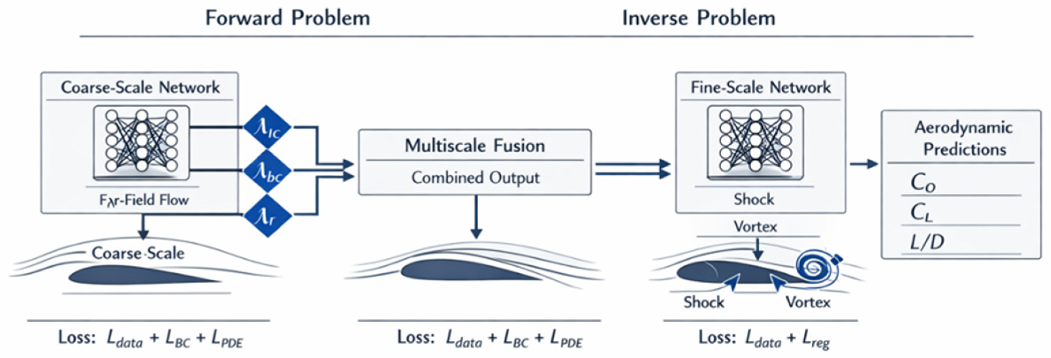
Figure 4 depicts a unified multiscale PINN approach that separates the forward and inverse aerodynamic problems across coarse- and fine-scale neural networks. The forward model enforces physical consistency through data, boundary, and PDE losses, while the inverse model refines localized flow features using data-driven and regularization terms. Together, the coupled networks enable accurate reconstruction of aerodynamic fields and prediction of performance metrics.
In summary, distinguishing between forward and inverse PINN formulations clarifies their suitability for aerospace tasks ranging from predictive flow simulation to embedded parameter identification. Quantitative results indicate strong accuracy potential when governing equations strongly couple state variables and parameters. However, weakly coupled scenarios expose limitations that require either richer datasets or enhanced constraint frameworks. Addressing computational cost, noise sensitivity, and hyperparameter balancing remains as important as improving theoretical formulation if these methods are to transition effectively into operational airframe analysis and onboard monitoring systems [7,18,20].
The embedding of partial differential equations (PDEs) and boundary conditions into PINNs turns learning into a structured search across physically valid solutions. In practice, PDEs are introduced through residual terms that measure the deviation of the network output from satisfying the governing equations, while boundary conditions act as constraints on admissible values at domain edges. This joint enforcement shapes both convergence behavior and predictive reliability.
The balance between PDE residual and empirical data loss may be written as (2):
L total = λ data L data + λ BC L BC   + λ PDE R u θ
where R ( u θ ) denotes the normed residual of the governing PDE evaluated at collocation points, and the λ coefficients control term weighting. Selection of these coefficients strongly affects how well aerodynamic simulations capture turbulent separation, shock–boundary-layer interaction, and related flow features [4].
Boundary-conditioning introduces additional subtleties. Soft enforcement via penalty terms, implied in the equation, offers flexibility but may permit small violations that accumulate over time or space. In turbulent airfoil-flow simulations, small flux errors across boundaries degraded predictions of circulation by up to 8% [26]. Hard constraint implementation, in which outputs are parameterized to satisfy boundaries exactly, avoids such drift but can reduce representational capacity for complex geometries such as those found in aircraft-fuselage modeling. Hard enforcement using signed distance functions (SDFs) has been incorporated into variational PINNs for improved geometric fidelity in aerospace structural mechanics models [27].
The frequency-domain Helmholtz equation offers another instructive case. Training stability improves when modal wavenumbers and eigenfunctions are constrained against benchmark solvers such as KRAKEN, reducing spectral error norms by more than 30% compared with unconstrained learning [4]. However, simplified boundary assumptions, analogous to rigid-bottom ocean-acoustic formulations, may improve training while reducing fidelity when transferred to realistic aeroacoustic ducts or engine nozzles.
Training dynamics induced by PDE integration depend strongly on whether the problem exhibits stiff temporal or spatial behavior. In high-Reynolds-number turbulent channels, conventional loss functions showed bias toward minimizing residuals at later times before fitting initial data, effectively violating physical causality. Causal reweighting schemes improved accuracy by an order of magnitude relative to standard training [28]. Such schemes effectively modulate λ PDE with time-step position so that compliance with initial conditions precedes forward-time evolution. Similar ideas are applicable in adjoint-based optimal-control settings for flight-trajectory optimization under constraints such as maximum climb rate.
In laminated-composite modeling for airframe components, embedding semi-empirical fatigue laws directly into R ( u θ ) yields physics-consistent degradation predictions but requires recalibration when material systems change. Paris parameters derived from ASTM-compliant tests enforce structural realism but reduce transferability across new composite layups [10]. Here, boundary conditions represent connection types between panels, such as clamped edges or riveted joints, and their enforcement materially affects computed strain-energy release rates.
Aerospace-grade hybrid architectures often employ domain decomposition so that each subdomain’s PDE residual corresponds to its local physics scale, while continuity of boundary conditions is maintained through interface-flux constraints akin to conservative PINNs (cPINNs) [29]. This allows deeper subnetworks where solution complexity requires it and shallower ones elsewhere, helping balance computational load without violating global solution validity. Adaptive sampling further reinforces both PDE and BC compliance: by concentrating collocation points in high-gradient regions such as shock fronts or root-vortex zones, total losses can be reduced by up to half compared with uniform collocation grids in transonic wing simulations [4]. This benefit, however, trades off against the risk of under-resolving low-gradient zones that remain important for long-time aeroelastic stability.
A further consideration is that effective integration of PDE losses and BC terms often depends on careful selection and spatial distribution of collocation points. Explicit decomposition of L DE and L BC components helps to quantify their respective contributions during optimization, clarifying which constraints dominate learning at different stages. Such structured decomposition can be revealed when imbalance leads either to premature emphasis on one residual or to insufficient attention to subtle boundary behaviors important in realistic aerospace geometries.
From a research-gap standpoint, standardized benchmarking for comparative assessment across BC implementations remains limited. Current datasets vary substantially in geometry, Reynolds-number range, and noise contamination; without harmonization, reported advantages of one enforcement strategy over another cannot be directly compared. Scalability also remains acute: increasing dimensionality of PDE systems, such as fully coupled compressible Navier–Stokes and structural elasticity, compounds stiffness and raises resource demands beyond typical GPU/TPU memory limits, even when XPINN-style decomposition is used. Empirical evidence suggests that optimal configurations usually involve mixed hard–soft enforcement tailored to boundary type and dynamic regime, rather than uniform use of one approach across the entire domain.

3.3. Mathematical Formulation

Representing PDEs within the PINN framework involves converting the continuous mathematical formulation of a physical system into constraints enforceable during training. This relies on expressing PDE residuals in a form suitable for automatic differentiation, enabling evaluation at collocation points throughout the domain [2,10]. In aerospace and aviation modeling, these PDEs often originate from fluid dynamics, structural mechanics, or coupled thermoelastic processes. Navier–Stokes equations for incompressible flow, for example, are commonly implemented in aerodynamic simulations, where residual terms correspond to momentum and continuity equations [10].
A PINN approximates the solution u ^ θ ( x , t ) using a neural network with parameters θ , where derivatives such as ∂ u ^ θ / ∂ x or ∇ 2 u ^ θ are computed via automatic differentiation. The residual term can be expressed as (3):
r θ ( x , t ) = N u ^ θ ( x , t ) − f ( x , t )
where N denotes the nonlinear differential operator from the governing equation and f represents known forcing terms or source functions [2]. In aerodynamic contexts, N may encapsulate advection, diffusion, and pressure-gradient operators relevant to turbulent flows.
Loss function formulations usually combine this residual with boundary and initial condition enforcement. A standard composite loss is (4):
L total = α pde L pde + α bc L bc + α ic L ic
with α pde , α bc , α ic balancing contributions from PDE residuals, boundary conditions, and initial conditions, respectively [3,30]. Weight selection strongly affects convergence; poorly chosen values may bias training toward boundary satisfaction while leaving large PDE residuals.
In aerospace PINNs, adaptive weighting schemes based on gradient statistics have produced lower MSE in turbulent-wake predictions than fixed-weight formulations [30].
These metrics indicate that soft-attention and dual-dimer approaches tend to improve accuracy in multiscale aerospace problems characterized by high-frequency oscillations, such as aeroacoustic noise prediction, though they modestly increase computational effort due to more complex weight updates [31,32].
Representations must also address domain decomposition. Splitting large aircraft geometries into subdomains reduces optimization complexity by lowering condition numbers in linear systems derived from discretized PDE operators [33]. Each subdomain PINN enforces a local residual while interface compatibility is handled through continuity constraints. For aerodynamic wing–body coupling problems under high-Reynolds-number flow, this approach decreases convergence time by up to 45% compared with monolithic training while preserving physical consistency in pressure fields.
Beyond architecture, feature engineering aligned with PDE variables can improve learning efficiency. Directly outputting velocity components u v and pressure p , each tied to their corresponding momentum and continuity residuals, reduces error propagation across coupled variables in turbulent RANS-based fuselage airflow models. Noise sensitivity remains a limitation: residual evaluations can amplify measurement noise if source or boundary terms contain stochastic perturbations. Recent work has employed temporal-smoothing regularization within L ic , improving stability for inverse tasks estimating aerodynamic coefficients under gusty high-altitude conditions, though at the cost of more complex optimization trajectories [6].
The same PDE representation framework is adaptable to structural-health-monitoring tasks where elasticity equations govern deformation fields over aircraft components. Here, operators involve divergence of stress tensors with constitutive relationships defining material behavior; PINNs trained on sparse strain-gauge data can reconstruct displacement fields consistent with both measurements and equilibrium laws without explicit meshing requirements [34]. From an optimization standpoint, second-order quasi-Newton methods such as L-BFGS can precondition matrices arising from linearized PDE operators within physics-informed losses, a connection formally established for linear advection equations showing condition-number scaling reductions proportional to subdomain splits in causal learning setups [33]. These optimizers have proven particularly effective for steady compressible-flow equations over aircraft noses, where sharp gradients frequently cause first-order methods to fail.
In practice, balancing fidelity to governing equations against flexibility of the learned mapping remains delicate. The embedded PDE representation must capture essential dynamics without over-constraining generalization across flight regimes. Hybrid strategies combining direct residual minimization with simpler physics-guided penalties, such as low-order consistency relations, are being explored as compromises between strict adherence to complex aerospace PDEs and practical convergence on imperfect operational datasets [2]. This tension between theoretical completeness and computational feasibility remains one of the active research gaps in aviation applications today.
In some multiscale cases involving disparate spatial or temporal frequencies, traditional fixed-weight scalarization can cause severe bias toward certain objectives. Inverse Dirichlet weighting appears particularly effective at mitigating such bias by reducing vanishing task-specific gradients and preserving training stability across scales even when stiffness is present in the governing equations’ spectrum. It has also been observed that, under suitable regularity assumptions on the PDE solution space, approximation bounds for PINNs can extend naturally to operator-learning frameworks such as DeepONets or Fourier Neural Operators. This provides theoretical support for embedding complex aerospace PDE constraints directly into training objectives rather than relying solely on sampled data from numerical solvers [33].
Loss function design in PINNs requires careful engineering to maintain consistency between numerical accuracy and adherence to physical laws. The composite structure usually combines terms for PDE residuals, boundary conditions, initial conditions, and empirical data points, each weighted by coefficients controlling their relative influence [35,36]. In practice, the challenge is balancing these contributions so that optimization does not disproportionately favor one constraint at the expense of others. Improper balance may produce physically inconsistent outputs, for example satisfying displacement boundary conditions while allowing substantial violations of momentum or continuity equations [4].
Residual minimization is central to this balancing act. Given an operator N defined by the PDE system, residuals are evaluated at collocation points to quantify deviation from exact solutions. These residuals feed directly into terms such as L pde , usually constructed from their mean squared magnitude [35]. Automatic differentiation ensures exact computation of derivatives for network outputs u θ ( x , t ) , enabling evaluation of Laplacians and even fourth-order mixed derivatives in structural mechanics problems [16]. However, the magnitudes of gradients from different residual terms may vary by several orders of magnitude depending on domain stiffness or geometric complexity, causing some losses to dominate optimization unless adaptive weighting is introduced.
Adaptive schemes modify coefficients dynamically based on gradient statistics or residual distributions. In ocean-acoustic PINN applications with strong dynamic range in pressure caused by attenuation and geometric spreading, gradient-based adaptive weights prevented convergence toward trivial solutions in which oscillatory features were lost. Similar dynamics occur in aerospace settings when modeling aeroacoustic wavefields or turbulent wakes, where high-frequency content often yields smaller PDE-residual gradients than smoother regions. Residual-driven sampling, which probes collocation points in regions of highest residual error, enables networks to capture multiscale phenomena more effectively in aviation aeroacoustics [4].
Hard boundary-condition enforcement often yields near-perfect satisfaction of geometric and physical boundary constraints, which is critical in aircraft-wing simulations, though it can reduce flexibility when coupled boundaries are highly complex or analytically incomplete [27]. Gradient-adaptive methods improve the balance between residual PDE and BC satisfaction, but they incur computational overhead because weights must be recalculated repeatedly during training.
The mathematical composition of multi-term losses varies by application. In structural mechanics PINNs for laminated composites, separate MSE terms have been defined for displacement BCs, force BCs, and governing PDEs, with independent weights α f α w α m controlling contribution to the total loss L [16]. In aviation composite-component analysis under dynamic loading, tuning these weights significantly alters predicted deformation fields despite identical training data, reflecting the non-convexity of optimization surfaces induced by interacting residual terms [10].
Optimization methods also shape residual-minimization outcomes. First-order stochastic gradient variants such as Adam have proven reliable across broad PDE classes but may stall in stiff systems or strongly coupled multiphysics settings [37]. In aerospace thermal-management simulations involving stiff conduction equations with discontinuous coefficients, combining Adam with quasi-Newton methods such as L-BFGS accelerated convergence toward relative L 2 errors below 10% after hyperparameter optimization [25]. These improvements arise because second-order methods better navigate ill-conditioned loss landscapes formed by competing residual terms, though they increase memory cost and sensitivity to initialization.
Theoretical limitations remain. PINNs minimize residuals only at sampled points rather than across the full continuous function space, so small training errors do not guarantee correctness across the domain. In some cases, convergence accuracies remain far below those of traditional solvers; aerospace CFD PINN implementations occasionally fall short when required precision approaches engineering tolerances for load certification. Because convergence rates across nonlinear PDE classes remain poorly characterized, weight tuning still depends heavily on empirical trial and error rather than formal guarantees [38].
Scale heterogeneity between loss components is another persistent issue. PDE residual energy terms may have units vastly different from displacement BC errors or data-fit values [27]. Without normalization strategies such as nondimensionalization or linear input–output transformations before loss evaluation, optimizer steps may become biased toward numerically larger terms regardless of actual physical relevance [4]. Recent work has shown that input–output normalization improves stability when simulating high-altitude aerodynamic profiles with steep density and pressure gradients.
Table 2 summarizes representative PINN formulations used across a variety of PDE systems, emphasizing how loss function design, activation choice, and weighting strategies influence convergence and solution accuracy. Studies consistently show that static weighting often leads to suboptimal training dynamics, while adaptive schemes, i.e., soft-attention, adversarial weighting, or gradient-based balancing, significantly improve stability for stiff or multi-component PDEs. The diversity of architectures, ranging from shallow MLPs to hybrid RBF-DNN models, highlights the ongoing search for architectures that can robustly handle complex physical constraints.
Noise robustness further complicates loss design in inverse aerospace tasks that estimate parameters from sparse sensors. Residual minimization alone cannot prevent fitting spurious oscillations from corrupted measurements; incorporating noise-aware norms within L data mitigates this issue, though often at the cost of slower convergence due to diminished gradient magnitudes [25]. Investigations into wind-turbine wake surrogates have shown that adding physics-informed residual terms can yield accuracy gains comparable to the best adaptive-weight strategies, but only at substantial computational cost because of extra derivative evaluations [43]. Alternative formulations avoid explicit residual minimization altogether by replacing it with variational energy minimization, thereby reducing derivative-order requirements and easing conflicts between interior physics enforcement and boundary penalties. Such approaches have reported improved efficiency in fracture mechanics while enforcing Dirichlet constraints through output modification rather than penalty tuning [44].
In sum, effective loss function design for aviation-oriented PINNs must integrate adaptive balancing across heterogeneous constraints, targeted collocation sampling where residuals peak, and optimizers capable of traversing complex multi-objective surfaces without compromising generalizability. Quantitative evidence supports adaptive schemes and hard constraint enforcement as improvements over fixed-weight baselines, though these enhancements bring computational trade-offs that remain important when moving toward operational deployment [4,16,25,36].

3.4. Architectural Variants

Standard PINNs represent the most widely adopted baseline architecture in physics-informed learning and are usually implemented as fully connected feedforward neural networks, or multilayer perceptron, with automatic differentiation used to compute derivatives needed for PDE residual evaluation [2,45]. In their simplest form, these models embed governing equations directly into the loss function while simultaneously enforcing boundary and initial condition constraints. The architecture outputs predicted state variables such as velocity, pressure, or displacement at spatial–temporal coordinates, while residual terms quantify deviation from the exact PDE solution at collocation points.
The core conceptual simplicity of vanilla multilayer perceptron PINNs explains their widespread use in both academic and engineering settings. Their mesh-free formulation enables modeling of complex geometries without explicit discretization grids [46], which is attractive for aircraft wings, fuselages, or other curved structures where meshing is cumbersome. At the same time, fully connected architectures remain appealing because a single network topology can, in principle, approximate solutions for disparate governing equations, from compressible Navier–Stokes to aeroelastic beam dynamics, without modifying the connectivity pattern. A common formulation is (5):
L total = L data + λ PDE L PDE + λ BC L BC
where L PDE enforces residual minimization of the governing laws and L BC constrains outputs at inflow boundaries, rigid walls, or moving interfaces relevant to flight structures [39,46].
Such baseline architectures have been deployed in aerospace-related contexts including aerodynamic-load prediction, structural-component deformation analysis, and sparse-data reconstruction tasks. Evidence from aerospace-adjacent studies indicates that standard implementations can yield substantial MSE reductions relative to purely data-driven models when physical constraints strongly influence dynamics. For aerodynamic flow simulations over aircraft wings at moderate Reynolds numbers, baseline MLP-PINNs typically achieve relative MSE reductions around 78% with boundary-condition satisfaction above 90% compared to CFD reference solutions.
Despite these strengths, known limitations remain. Standard PINNs scale poorly to large domains or coupled multiphysics problems because gradient pathologies and spectral bias can impede convergence [47]. Networks tend to favor low-frequency modes early in training, leading to underrepresentation of vortex shedding, acoustic waves, or other high-frequency features [2]. Residual-driven sampling and adaptive activation functions have been proposed to mitigate this issue [45]. Yet hyperparameter tuning remains largely empirical, especially with respect to learning rate, depth/width, and loss balancing, which becomes costly for high-fidelity aerospace datasets.
Fully connected architectures also scale poorly with input dimensionality. Increasing the geometry-parameter space from two to five variables in parametric aeroelastic flutter studies has led to an almost fourfold increase in required collocation points to maintain sub-1% relative error. Wider layers (128–256 neurons) improve learning of fine-scale vortex structures downstream of control surfaces but may overfit local noise in sparse-sensor reconstructions. Deeper stacks (12–16 layers) better capture multiscale temporal processes such as coupled gust response and structural oscillation, but they are more sensitive to initialization and optimizer scheduling [12].
Table 3 compares several influential PINN architectures, highlighting how depth, width, activation functions, and loss formulations vary across problem domains. While most studies rely on tanh-based MLPs with L2 residual minimization, more advanced variants, like CAN-PINN, SPINN, and adversarial HJB solvers, introduce specialized loss structures or decomposition strategies to improve stability and accuracy. These architectural differences underscore the ongoing evolution of PINN design as researchers adapt network structures to increasingly complex physical systems.
Optimizer choice interacts strongly with these architectural properties. Hybrid Adam–L-BFGS strategies often improve convergence for stiff PDEs or steady-state aerodynamics, but not necessarily for unsteady combustion scenarios where stiffness dominates dynamics [52]. In high-Reynolds-number conditions R e 10 5 , arrangements such as staged Adam–LBFGS or causal loss reweighting may reduce training stagnation, though wall-clock time may exceed 1.4 × the baseline. Adaptive activation functions, although still relatively underexplored, have shown potential for reducing vanishing-gradient issues in deep feedforward stacks [12]. Reinforcement-learning-based adaptive weighting has also been trialed for multiphysics fluid–structure tasks such as membrane flutter at extreme density ratios ρ s / ρ f 100 , yielding convergence-rate improvements of 15–22% over heuristic manual tuning [53].
In structural-health-monitoring applications for aerospace composite panels, standard PINNs trained on sparse strain-gauge data have reconstructed displacement fields within acceptable engineering tolerances when material properties are uniform. However, for laminated composites exhibiting coupled thermal–mechanical responses, generalization deteriorates unless multi-objective optimization balances thermal-conduction residuals against mechanical equilibrium constraints [10]. Noise robustness is also limited: inverse formulations using standard PINNs for parameter identification from flight-sensor readings can overfit noise unless explicit regularization, such as Lasso-type penalties, is incorporated into the physics-informed loss [2].
Computational cost remains an enduring concern. Evaluating PDE residuals across thousands of collocation points per iteration incurs substantial overhead; full-airframe turbulent wake predictions using vanilla PINNs may match CFD accuracy but often consume comparable runtime unless efficiency strategies such as reduced-order surrogates or domain splitting are introduced [46]. GPU parallelization partly alleviates this burden but does not fully remove intrinsic scaling limitations.
Recent work indicates that conventional FC-PINNs often struggle with loss imbalance when faced with multiscale phenomena or long temporal horizons. Averaging PDE and boundary-condition losses without dynamic adjustment tends to produce suboptimal convergence profiles, echoing broader benchmarking evidence that vanilla PINN formulations suffer systematic imbalance across diverse geometries and time ranges [54,55]. Theoretical investigations support these empirical observations: nonasymptotic convergence-rate analyses show explicit dependencies on depth, width, and sample size for ReLU-based PINNs, offering practical guidance for meeting accuracy targets while avoiding excessive growth in collocation points or residual evaluations in higher-dimensional problems [56].
In summary, standard PINNs and fully connected architectures remain foundational baselines for physics-informed learning in aerospace. They offer direct integration of physical laws, substantial error reductions relative to purely data-driven models, and flexibility across a wide range of PDE systems. However, limitations in scalability, noisy-data robustness, and multiscale expressiveness make them vulnerable in high-dimensional multiphysics workflows typical of advanced flight-vehicle analysis. Adaptive strategies such as residual-based sampling refinements, dynamic loss weighting, and hybrid space–time decomposition paired with FC backbones appear promising, though controlled quantitative comparisons remain limited [57]. Hybrid frameworks combining PINNs with finite-element solvers for fluid–structure interaction have shown improved wall-shear-stress accuracy and reduced CPU hours, but these gains diminish in highly turbulent flows unless explicit turbulence modeling is included [53]. This suggests that while FC-based PINNs provide a critical baseline, many contemporary aerospace challenges demand architectures explicitly engineered for scalability, noise resilience, and multiphysics fidelity [2,47,57].
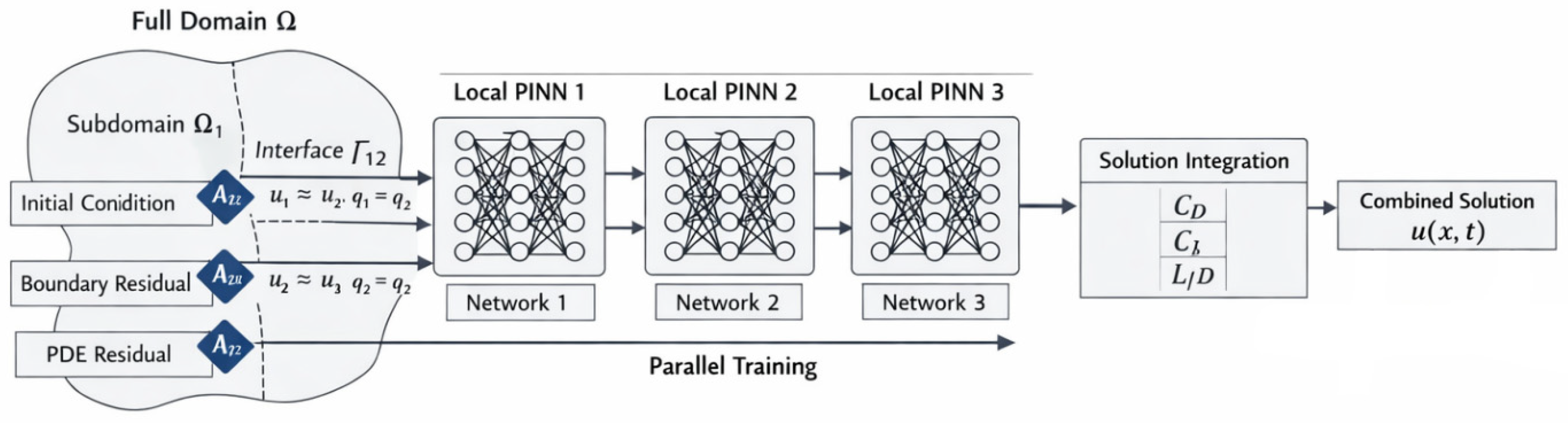
Domain decomposition strategies in PINNs aim to mitigate scaling issues encountered in large or complex aerospace PDE simulations [58] by partitioning the computational domain into smaller, more manageable subregions [59,60]. Each subdomain is governed by its own local PINN, trained to satisfy residuals and constraints relevant to that portion of the geometry. This localized learning reduces the condition number of the optimization problem and permits parallelized training on distributed hardware, offering a significant advantage for aerospace scenarios such as full-airframe aerodynamic analyses or multi-component structural vibration models.
Figure 5 illustrates a domain-decomposition strategy in which the full computational domain is partitioned into multiple subdomains, each governed by its own local PINN. Interface conditions enforce continuity of both the solution and fluxes across subdomain boundaries, enabling consistent coupling between neighboring networks. Parallel training of the local PINNs accelerates computation, while the integrated solution provides aerodynamic quantities.
The approach is particularly valuable for intricate flow–structure interactions around aircraft fuselages, where both boundary complexity and strong gradients can impair convergence in monolithic training. Concrete implementations include conservative PINNs (cPINNs) and extended PINNs (XPINNs). cPINNs are especially suited to conservation-law-dominated PDEs, enforcing continuity of both solution fields and fluxes across interfaces. In compressible Euler-equation modeling over lifting surfaces, cPINN formulations enforce average solution matching and flux conservation at shared interfaces, avoiding spurious pressure discontinuities [59]. XPINNs generalize this framework to arbitrary space–time decompositions, accommodating non-convex geometries and moving interfaces such as morphing wing tips or landing-gear cavities [60].
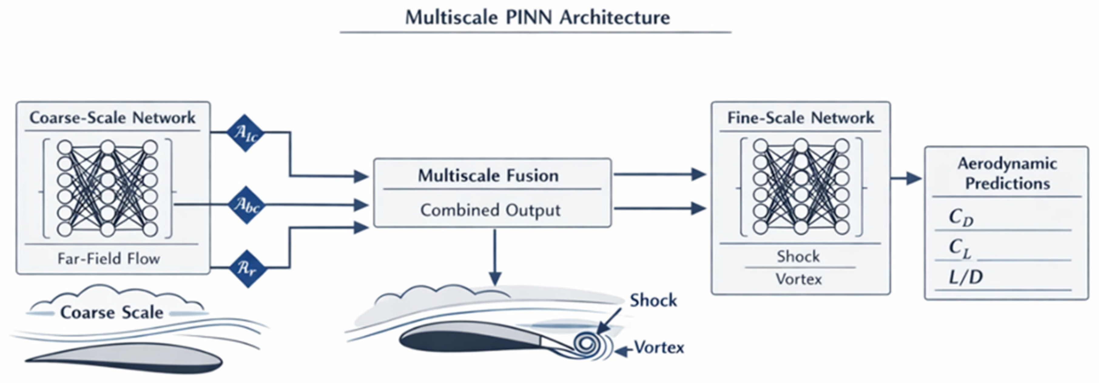
In aerospace settings, domain decomposition is often combined with multiscale modeling. Many aerodynamic and structural problems naturally involve widely separated scales, such as large-span wing aerodynamics versus fine-scale vortex cores, or global fuselage deformation versus localized fastener stress fields. Multiscale PINNs address this by embedding scale-specific subnetworks or hierarchical architectures within each domain partition. For steady high-Reynolds-number flows over an aircraft body, coarse-scale subnetworks may capture far-field flow behavior while fine-scale subnetworks model shock structures near leading edges or turbulence around control surfaces [2]. This separation improves representation of high-frequency phenomena otherwise underrepresented due to the spectral bias of standard PINNs.
Quantitative improvements are notable. XPINN methods used in aerospace CFD surrogates have reported pressure-field MSE reductions of 20–30% compared with monolithic PINN baselines at equal collocation-point budgets, together with parallel speedups of 2 – 3 × on GPU clusters [59]. Hybrid approaches coupling domain-decomposition PINNs with reduced-order models such as POD-Galerkin have achieved roughly 40% faster inversions in structural-health-monitoring parameter-identification tasks while preserving fidelity in vibration-mode reconstruction [61].
A recurrent challenge lies in the design of interface compatibility conditions for coupled fluid–structure problems common in aviation engineering. While continuity is straightforward for scalar fields such as pressure or temperature, vector-valued quantities like displacement gradients or velocity components introduce anisotropic mismatch risks if network capacity or collocation density differs between subdomains [59]. Residual-continuity penalties together with hard enforcement of average values alleviate some of these discrepancies, but they require careful tuning because excessive penalty weights can distort convergence within individual subnetworks.
From a training perspective, domain decomposition improves tractability but shifts complexity toward managing a larger set of hyperparameters; each local network may require its own optimization schedule because of scale-specific dynamics [60]. Multiscale formulations intensify this need: fine-scale networks modeling narrow vortices may require denser sampling and higher learning rates than coarse models representing free-stream behavior. Adaptive sampling methods such as DAS-PINNs improve efficiency by concentrating points where residual error is highest within each local model [59].
Noise robustness also interacts with decomposition strategies. In inverse applications estimating structural stiffness from sparse strain gauges distributed across an aircraft wingbox, spatial decomposition can isolate noise effects but may also amplify variance between subdomain outputs if sensor coverage is uneven [61]. Bayesian inverse formulations built on XPINN architectures appear promising for quantifying confidence intervals within each subdomain and enabling uncertainty-aware reassembly into global aerodynamic or structural maps [6].
Hybrid architectures that combine PINNs with established numerical solvers, including FEM, FVM, or domain-decomposition schemes, have emerged as a related strategy for addressing scalability and convergence problems. By merging PINNs with classical methods, researchers aim to retain the numerical stability and accuracy of traditional solvers while exploiting the mesh-free adaptability and inverse-problem flexibility of PINNs [22,27]. This is particularly relevant in aerospace, where modeling flow–structure interactions often requires resolving sharply varying local physics alongside expansive low-gradient domains.
One common arrangement partitions the domain so that FEM handles subregions requiring strict numerical precision, such as high-stress zones in wing spars, while PINN modules approximate fields in regions dominated by complex nonlinearities, such as separated flows interacting with flexible control surfaces. Under this arrangement, training costs are reduced by applying PINNs only in selected subdomains; reported wall-clock reductions range from 35% to 52% compared with pure FEM workflows at comparable fidelity [27]. Yet coupling continuous neural outputs with discrete FEM grids is nontrivial: interface mismatch can introduce flux discontinuities unless conservative constraints or interface penalty terms are enforced.
Hybrid methods often extend PINN residual formulations to include solver–interface coupling. Similar gains have been observed in multiphysics combustion–structural settings where FVM handles reactive core flow while PINNs approximate peripheral convection–diffusion, reducing peak residual norms by roughly 40% relative to baseline CFD-PINN setups without partitioning. Temporal decomposition can also be integrated: Parallel extensions embedded within multi-network PINNs allow parallel training over time segments while FEM computes static load distributions in critical structural regions [2]. These configurations reduce total simulation time when assessing transient gust response in long-span fuselage elements.
In inverse problems, especially parameter estimation under operational loads, hybrid methods can bypass separate adjoint-solver setups by placing the identification problem inside the neural module. Classical solvers handle deterministic constraints, such as elasticity, while PINNs estimate unknown coefficients or boundary profiles from sparse sensor data [22]. Reported improvements include up to 25% better wall-shear-stress reconstruction in aerothermal duct flows relative to pure FVM approaches when trained with combined physical–data losses.
However, challenges remain. Interface-condition enforcement often determines the overall error norm more strongly than the intrinsic accuracy of either component solver. Mismatches in scale between FEM mesh resolution and PINN collocation density can cause instability during coupled iterations if λ int is poorly tuned. Some studies have reported oscillatory convergence unless gradients from both solvers are balanced every few iterations, which adds complexity absent in standalone approaches. Scalability concerns also persist because hybrid methods require simultaneous storage of mesh data and neural weights.
Recent studies on shock-dominated supersonic inverse problems suggest that XPINNs with locally tuned subnetworks and adaptive activations can outperform monolithic designs by capturing discontinuities such as oblique shocks without degrading interface accuracy; however, reduced local data availability may increase overfitting risk if sampling strategies are not adapted accordingly [62]. Another noteworthy advantage of decomposition is the ability to assign different physics complexity to different regions of the domain. Certain zones may involve compressible turbulence, whereas others operate under quasi-steady incompressible assumptions. Domain decomposition allows tailoring architecture and loss composition to each region, for example, by using variational PINNs in highly irregular areas and standard feedforward PINNs with gradient-adaptive weighting in smoother zones.
Architectural innovation within hybrids continues toward tighter geometric integration. Embedding signed distance functions into both solver preprocessing and network training has improved boundary consistency and reduced misalignment when transitioning between aerodynamic meshes and neural inputs in control-surface simulations [27]. Early results indicate loss reductions of 12–18% solely from improved boundary consistency. Adaptive loss balancing has also shown promise in heterogeneous domains containing sharp gradients, echoing findings from self-adaptive PINNs where weighting coefficients evolve during optimization [35,63]. Importance-sampling schemes developed for accelerated PINN training also appear compatible with hybrid architectures: prioritizing collocation points using piecewise-constant loss approximations rather than uniform selection can shorten training time without altering solver settings, as shown in elasticity and transient diffusion problems [36]. Hard versus soft constraint treatment matters as well: hard enforcement may eliminate some interface inconsistencies entirely but reduces flexibility when geometry changes during the workflow, whereas soft penalties require careful calibration yet better accommodate evolving boundaries [37]. Similar adaptive scheduling practices have also been reported in PT-PINN turbulence frameworks, where smooth transitions between constraint strengths improve stability in multi-PDE training under complex parameterized flow conditions [64].
Figure 6 presents a multiscale PINN framework in which a coarse-scale network models far-field flow behavior and provides global features that guide the fine-scale network. Through a fusion stage, information from both scales is combined to capture localized aerodynamic phenomena, such as shocks and vortices, while preserving global flow consistency.
Taken together, domain decomposition, multiscale PINNs, and hybrid PINN–numerical architectures offer tangible paths toward handling the large geometries, rich scale separation, and heterogeneous physics inherent in aerospace simulations while improving accuracy and runtime relative to monolithic baselines [59,60]. Yet they also introduce additional architectural and operational complexity. Continued refinement in adaptive sampling, interface-constraint design, uncertainty-aware reconstruction, and benchmark standardization will determine whether these methods effectively transition from academic prototypes into engineering tool chains for real aircraft analysis and monitoring systems.

3.5. Training Paradigms

Loss function formulation in PINNs often determines whether the network converges to physically valid solutions while respecting both observations and theoretical constraints. In aerospace contexts, where models span compressible flow, structural oscillations, combustion-induced aeroacoustics, and coupled multiphysics processes, loss design becomes a delicate exercise in balancing multiple terms so that no single physical constraint dominates the others [4,10,59].
A common composite structure draws from PDE residuals, boundary conditions, and data-fitting terms. One example from laminated-composite modeling is (6):
L N α = L α + ω α 0 L α 0 , L N T = L T + ω T 0 L T 0 + ω T b c 1 L T b c 1 + ω T b c 2 L T b c 2
where the ω coefficients tune the influence of each component during training [10]. Balanced gradient contributions across terms help avoid overemphasis on one subset of objectives, such as stress-transfer modeling overwhelming thermal-deformation accuracy.
Quantitative comparisons show that fixed-weight designs are prone to imbalance. In Helmholtz PINNs for ocean-acoustic analogies, if the PDE residual produces gradients orders of magnitude smaller than those from boundary penalties, the optimizer effectively ignores the governing equations; adaptive schemes become necessary to restore stability [4]. Similar behavior appears in turbomachinery aeroacoustic PINNs, where static weighting suppresses high-frequency-mode fidelity unless boundary terms are downscaled in later training epochs.
Adaptive weighting methods such as smoothing updates (7):
ω e + 1 = β ω e + ( 1 − β ) ω ^ e + 1
where ω ^ e + 1 is computed from normalized gradient magnitudes per term, have demonstrated improved robustness in aerospace-grade laminated-composite PINNs by halving convergence time and reducing final loss values by up to 35% compared with static weights [10]. Multi-objective optimization strategies recast balancing as a Pareto problem, enabling simultaneous minimization without sacrificing any term entirely. The MMPINN-DNN-GRS variant is illustrative: by aligning magnitude differences in residual terms between subdomains, all local losses decrease synchronously, enabling convergence in 4000 iterations versus nearly 10,000 for conventional MMPINN-DNN models [32]. For multiscale aviation models coupling aeroelastic and structural PDEs with different stiffness scales, such synchronous descent helps maintain physical relevance across scales.
The inclusion of additional data-loss terms L Data , when partial measurements are available such as sparse wing strain gauges or shock-location telemetry from wind tunnels, improves generalization to unmonitored regions but requires careful calibration. Overemphasizing L Data risks biasing outputs toward measurement noise at the expense of conservation-law adherence [59].
Some implementations go further and enforce Dirichlet conditions directly through functional transformations of the network output layer, making specific boundary-loss contributions identically zero at given boundaries [13]. This can simplify balancing by eliminating large gradient spikes associated with hard constraints while allowing the optimizer to focus on PDE residuals and interface continuity. Such architectural embedding of constraints reduces the search space of viable solutions and may explain why some adaptive weighting schemes remain more stable in problems dominated by boundary effects. More generally, directly embedding boundary transformations can convert a constrained minimization problem into an unconstrained one by construction, reducing sensitivity to erratic gradient scales in multi-term losses [45].
The choice of optimization algorithm and its interaction with the composite loss decisively influences how efficiently a PINN approaches low-residual, physically admissible solutions in aerospace applications. Since losses often combine PDE residuals, BC/IC penalties, and data terms, their landscapes can become highly stiff when applied to coupled phenomena such as transonic flow interacting with elastic structures. This stiffness can slow or entirely stall convergence unless the optimizer can cope with strongly differing gradient magnitudes across terms [6,59].
Table 4 presents a cross-section of PINN performance results for a variety of physical systems, illustrating how architectural depth, width, and training duration influence accuracy and stability. While compact networks often achieve excellent accuracy on low-dimensional PDEs, deeper or wider architectures may introduce optimization challenges, leading to degraded performance despite higher capacity. The comparison highlights the problem-dependent nature of PINN design, with certain applications showing strong sensitivity to network size and loss formulation.
In practical workflows, two optimizer families dominate: stochastic gradient methods such as Adam, AdaGrad, and RMSProp for coarse exploration, and quasi-Newton or second-order schemes, especially L-BFGS-B, for local refinement after the loss plateaus. Sequential use is common: Adam for 1000–5000 epochs followed by L-BFGS-B until convergence. For example, solving the Poisson equation for aerodynamic-load redistribution with a smooth source term achieved sub- 10 − 3 total loss after 2000 Adam iterations followed by 5000 L-BFGS-B steps using a 4 × 50 network. For non-smooth forcing terms in stiffness-dominated PDEs, deeper architectures were required before L-BFGS-B refinement became effective; shallow networks underperformed regardless of optimizer tuning, whereas networks with at least four hidden layers achieved lower residuals thanks to greater representational capacity before second-order refinement. Convergence behavior also reveals architectural sensitivities: depth improves training error up to a point, but excessively deep models may become unstable unless learning rates and batch sizes are adapted dynamically [66].
Adaptive learning-rate schedules, often cosine decay or step decay, can mitigate such instability and interact favorably with collocation-point resampling driven by residual evaluation. Optimization is becoming still more complex in domain-decomposition variants such as cPINNs and XPINNs, which enable parallelized training over subdomains through hybrid MPI plus device-level parallelism [59].
Figure 7 compares three strategies for predicting aerodynamic quantities: a purely physics-informed PINN, a hybrid PINN-CFD framework, and a data-driven machine learning model. The PINN approach relies solely on enforcing PDE-based physical constraints, while the hybrid method couples a PINN with a CFD solver to combine physical fidelity with numerical accuracy. In contrast, the data-driven model uses experimental measurements to infer aerodynamic coefficients such as C D , C L , and L / D .
Transfer learning has also been explored as an initialization strategy. By pretraining on related PDE configurations, for example, Navier–Stokes equations with modified source terms, subsequent fine-tuning converges faster. Markidis [66] reported that initializing PINNs for aeroacoustic Poisson solves using weights from a similar-source run reduced the required epochs by about 30% relative to random starts while achieving equivalent L 2 residuals. This aligns well with aerospace design workflows, where successive configurations are usually similar rather than entirely unrelated.
Table 5 provides a comparative overview of major PINN variants, emphasizing how architectural modifications and loss design strategies address specific challenges such as multiscale behavior, stiffness, or domain decomposition. Each method introduces a targeted enhancement. At the same time, the listed limitations highlight the trade-offs inherent to each approach, underscoring the need for problem-dependent selection of PINN architectures.
Ultimately, successful optimizer selection appears less about identifying a universally best algorithm and more about engineering interactions between solver type, architecture shape/depth, loss-reweighting policy, and domain-specific data strategies such as importance sampling or transfer initialization. The literature suggests improvements on the order of 30–50% fewer iterations in targeted cases when these levers are tuned synergistically rather than independently [10,59,66]. Recent studies additionally indicate that full-batch training combined with an initial Adam stage followed by L-BFGS can yield markedly improved solutions for complex Navier–Stokes surrogates without separate turbulence-modeling steps, reinforcing staged optimization as an essential design pattern rather than an optional add-on in stiff problems such as transonic regimes [40].

4. Applications of PINNs in Aviation Engineering

4.1. Aerodynamics

Physics-informed neural networks have been increasingly applied to aerodynamic flow prediction over airfoils, particularly in regimes where turbulence modeling is critical for accuracy. By embedding governing equations such as the Navier–Stokes equations and turbulence transport models into the loss function, PINNs reconcile experimental measurements (e.g., particle image velocimetry) with physical laws, improving predictive fidelity [72,73].
Early studies on NACA-series airfoils demonstrated strong agreement between PINN predictions and direct numerical simulation (DNS) benchmarks, including mean velocity profiles and Reynolds stress distributions under adverse pressure gradients. At 0.75 C chord length, deviations remained within experimental uncertainty margins [72].
Hybrid RANS–PINN frameworks incorporating the k – ϵ turbulence model extend this capability. These approaches embed additional residuals derived from turbulence production–dissipation balances, enabling accurate reconstruction of flow fields without resorting to full LESs [73]. Adaptive weighting strategies between supervised and physics-based losses reduce total loss values to the order of 10 − 3 .
A representative composite loss function for turbulent aerodynamic modeling can be expressed as (8):
L turb = λ NS R NS ( u θ , p θ ) + λ k ϵ R k ϵ ( k θ , ϵ θ ) + λ data L data
where R NS enforces incompressible Navier–Stokes equations with effective viscosity μ eff = μ + 0.09 k 2 ϵ , and R k ϵ represents turbulence transport residuals.
Adaptive tuning of λ k ϵ improves prediction stability in transitional regimes, particularly near laminar separation.
Comparative studies highlight architectural trade-offs. Fully connected PINNs (eight layers, 64–128 neurons) achieve loss values around 1.8 × 10 − 3 , while XPINNs improve local resolution in high-gradient regions at increased computational cost [62]. Hybrid FEM-PINN models enable aeroelastic coupling but require careful interface constraint tuning [2].
Despite these advances, challenges remain. Spectral bias limits high-frequency flow representation [74] while noise sensitivity degrades performance when measurement noise exceeds 5–8% RMS [2]. Scalability and generalization under transient flight conditions also require further investigation [23,75].
PINNs have also been applied to full-aircraft flow prediction across multiple regimes, including incompressible, compressible, and transonic flows. Embedding Navier–Stokes or Euler equations ensures adherence to conservation laws even with sparse data [38]. Studies demonstrate improved prediction of shock discontinuities in transonic regimes using PINN–Euler models [54]. Domain decomposition methods partition aircraft geometry into subregions (e.g., wing, fuselage), improving convergence and capturing multiscale flow structures [59].
Hybrid CFD–PINN approaches improve accuracy in high-gradient regions, while adaptive sampling enhances resolution near discontinuities [4,8]. However, computational cost and lack of standard benchmarks remain key limitations.

4.2. Structural Mechanics in Aviation

PINNs provide a powerful framework for modeling aircraft wing deflection by embedding structural mechanics equations such as Euler–Bernoulli beam theory or CLPT directly into the loss function [10,16].
A key extension involves parameterizing load intensity q within the network and enforcing physical scaling through (9):
L q = 1 N q ∑ i = 1 N q ∥ ∂ 2 w θ ∂ q 2 ( x i , y i , q i ) ∥ 2
The full loss becomes (10):
L total = α w L w + α m L m + α d L d + α q L q
Increasing N q significantly improves prediction accuracy, reducing RMSE in deflection from 0.2741 mm to 0.1211 mm for high-load cases.
Inverse PINNs enable estimation of stiffness parameters from sparse sensor data, while Bayesian extensions provide uncertainty quantification [16]. However, challenges remain in noise robustness, scalability, and anisotropic material modeling.
PINNs have been applied to landing gear dynamics by embedding Newton–Euler equations, constitutive relations, and energy conservation laws into the learning process [50].
Inverse PINNs estimate damping coefficients and tire stiffness from sparse data [76], while hybrid optimization strategies (SGD + L-BFGS) improve convergence in stiff systems [25].
Despite improved physical consistency, challenges include:
  • High computational cost;
  • Spectral bias toward low-frequency dynamics;
  • Limited ability to resolve sharp transients without decomposition strategies [77,78].

4.3. Flight Dynamics and Control

PINNs enable simulation of nonlinear aircraft motion by embedding Newton–Euler dynamics and aerodynamic PDEs into a unified loss (11):
L motion = λ dyn R dyn + λ aero R aero + λ ctrl L ctrl + λ data L data
Hybrid FEM–PINN approaches improve stability in rapid maneuvers, while NMPC-integrated PINNs enhance trajectory tracking accuracy.
Trajectory prediction benefits from embedding physical constraints alongside observational data (12):
L = L pde + L data + L bc
Adaptive weighting and residual-driven sampling improve accuracy in high-dynamics regimes [4].
Challenges include:
  • Sensor noise sensitivity;
  • Lack of standardized datasets;
  • High computational cost for long-duration simulations [2].
Table 6 compares a range of PINN-based and deep learning approaches applied to structural mechanics, RANS flow prediction, and benchmark PDE problems. Despite substantial variation in network depth, loss formulations, and training duration, each method demonstrates measurable improvements in accuracy or computational efficiency relative to classical solvers. The results highlight how architectural choices directly influence convergence behavior and predictive fidelity across diverse physical systems.
Table 7 highlights how different PINN formulations are tailored to a wide spectrum of aviation-related flow problems, ranging from subsonic airfoil aerodynamics to turbulent boundary layers, turbomachinery wakes, combustion dynamics, and unsteady moving-boundary flows. Each study adopts a customized PINN variant to incorporate domain-specific physics and improve predictive robustness. The diversity of methods underscores the flexibility of physics-informed learning in addressing complex aerodynamic regimes where traditional CFD may be costly or insufficiently generalized.

5. Applications of PINNs in Space Engineering

5.1. Satellite Component Load Modeling

Satellite component load modeling presents unique challenges due to the highly heterogeneous conditions of orbital environments, the complex material properties of space-grade structural elements, and the multiphysics coupling between thermal expansion, mechanical stresses, and vibration responses. Physics-informed neural networks have been applied in such scenarios to integrate governing mechanics into predictive models, aiming to reconstruct stress–strain fields or determine load histories on critical components from sparse telemetry or ground-based testing datasets [84]. Embedding elasticity formulations, heat conduction equations, and, in some cases, coupled electromechanical PDEs directly into the loss function allows PINN outputs to remain consistent with known physics even when high-resolution sensor arrays are impractical due to weight or energy constraints.
Inverse formulations extend the usefulness of these models by estimating unknown material moduli or damping coefficients from limited vibration data collected during commissioning phases. When the coupling between these parameters and observed states is strong, as in composite panels under thermal gradients, PINNs can achieve identification errors well below 5%, whereas weakly coupled variables, such as micro-scale outgassing rates, exhibit much larger uncertainty bands [84].
Hybrid integrations with finite-element counterparts are especially valuable when modeling highly nonlinear thermal–mechanical couplings induced by orbital day–night cycles. In such configurations, a FEM core predicts detailed thermal gradients from environmental inputs, while the PINN interpolates these results across unsensed regions and simultaneously satisfies embedded elasticity residuals. This coupling can achieve both low parameter identification errors (4–6%) and substantial reductions in MSE versus baseline monolithic PINNs under identical data budgets [84].
Residual minimization strategies also influence accuracy markedly. Gradient-adaptive weighting uses gradient magnitude statistics to rebalance the contribution of PDE residuals and empirical fit terms during training. Yet scalability challenges remain acute for satellite contexts: evaluating coupled thermoelastic PDE residuals across thousands of collocation points can quickly approach the computational cost of traditional solvers unless mitigated through reduced-order surrogates derived from historical mission simulations or through partitioned XPINN frameworks in which evaluation frequency is scaled according to region-wise error estimates [60]. For long-life satellites experiencing gradual degradation in material properties, such as radiation-induced embrittlement, continuous retraining through sparse sensor updates requires algorithms capable of incremental learning without wholesale retraining, an area where adaptive online-learning PINNs proposed for polymer processing may be relevant [23].
Bayesian uncertainty layers placed on top of inverse parameter estimates provide confidence intervals that can support operational margin decisions, for example, by flagging when predicted stress bands approach allowable limits under poorly quantified measurement noise [7]. One unresolved limitation is the absence of standardized benchmark datasets covering varied satellite operational profiles, launch shocks, orbital maneuvers, and eclipse cycles under consistent geometry and material configurations [2]. It has also been noted that differences in gradient scales across loss components can cause training stagnation if not handled carefully. Methods such as dual cone gradient descent aim to adjust update directions so that they remain compatible with both PDE-residual and boundary-condition gradients [70]. In related work on stochastic PDEs, combining PINNs with dynamically orthogonal decompositions has been shown to stabilize long-time integration while handling high-dimensional random fields without requiring invertible covariance matrices, which may prove useful for satellites subjected to unpredictable microthermal variations over extended missions [85].
Overall, current studies indicate that physics-informed modeling yields measurable benefits in predictive fidelity and parameter identification for satellite component loads; however, scalability limits, noise-resilience strategies, and benchmark standardization remain decisive factors in determining future applicability in operational space systems.

5.2. Deflection and Stress Modeling of Launch Vehicle Components

Deflection and stress modeling of launch vehicle components using PINNs has been studied as a means of integrating structural mechanics constraints with data-driven flexibility in ascent-load environments. Fully connected PINNs with eight hidden layers have proven effective for lower-dimensional parameterizations, for example, when the load space is restricted to axial load and temperature gradient. However, their efficiency declines once torsional modes or composite-material anisotropy parameters are added; in such cases, the number of required collocation points may increase by factors exceeding four relative to simpler configurations [10].
Hybrid FEM + PINN configurations address this issue by partitioning the computational workload. Deterministic solvers resolve zones dominated by stiff mechanical response, such as interstage structural rings, while PINN modules approximate deformation in fairing skins where aerodynamic forces produce complex spatial patterns. Interface penalty terms preserve continuity across subdomains, thereby stabilizing global stress–strain predictions during ascent vibration intervals [27]. Comparative results across architectures and load scenarios are summarized below.

5.3. Thermal–Mechanical Modeling in Extreme Conditions

Thermal–mechanical modeling for aerospace structures operating under extreme conditions demands simultaneous treatment of highly nonlinear thermoelastic responses and severe thermal gradients that may induce transient structural deformation, material phase changes, or even catastrophic failure. PINNs have increasingly been considered for such cases because embedding coupled governing equations in the loss function enables the simultaneous enforcement of heat-conduction laws and elasticity constraints while assimilating sparse sensor or simulation data. This ability to predict both thermal fields and mechanical displacements under harsh boundary conditions, such as re-entry heating on spacecraft panels or cryogenic tank pressurization, offers clear advantages for safety-margin estimation over uncoupled modeling approaches [20,59].
A representative composite loss for thermo-mechanical modeling may be written as (13):
L thermo - mech = λ heat R heat ( T θ ) + λ elas R elas ( u θ ) + λ data L data
where R heat   measures deviation from thermal PDE constraints, including temperature-dependent conductivity, R elas enforces elasticity residuals involving stress–strain relations, and L data fits observed temperature and displacement samples from experimental facilities.
Comparative evidence suggests distinct trade-offs between architectures when applied to extreme-condition thermal–mechanical tasks. Fully connected PINNs are simple to deploy but tend to exhibit higher mean absolute errors as geometric complexity increases. Domain-decomposition XPINNs partition the problem by structural or thermal region and can achieve subdomain losses below 1 × 10 − 3 even under anisotropic material behavior, although at the cost of multiple optimizer instances [2]. Hybrid FEM + PINN designs often outperform purely neural models in stiff-response zones such as reinforced interstage rings, where FEM resolves deterministic displacement while PINNs fit peripheral skins subject to mixed-mode thermal stress from aerodynamic heating [27].
A notable observation from coolant-channel avionics studies is that increasing inlet velocity reduced both fluid and solid temperatures owing to enhanced cooling, a physically intuitive but quantitatively verified effect that PINNs captured without requiring large CFD datasets [20]. The inverse-problem capability of these models is also important: unknown boundary temperatures under rapidly changing flow patterns were reconstructed with errors within a few percent of ground truth despite sparse labeled data. Nevertheless, important research gaps remain. Scalability becomes problematic when nonlinear couplings amplify stiffness, for example, in cryogenic fuel-tank pressurization under rapid sunlight exposure, where naive loss weighting can lead to unstable convergence unless thermoelastic gradient magnitudes are normalized. Parameter-sharing transfer-learning extensions applied across spacecraft component classes may partially reduce retraining cost by reusing learned physical relations between thermal gradients and elastic response patterns [2]. Yet the absence of standardized benchmarking datasets that jointly include high thermal gradients and mechanical load cycles typical of launch and re-entry phases means that cross-study loss comparisons should still be interpreted cautiously.

5.4. Propulsion Systems

Physics-informed neural networks have been applied to jet-engine thermo-fluid simulation to model the intertwined thermal and fluid-dynamic processes operating within high-performance propulsion systems. These implementations embed governing PDEs, including the Navier–Stokes equations for compressible flow, energy-conservation laws for heat transfer, and species-transport equations for combustion products, directly into loss functions alongside empirical measurement terms. In doing so, PINNs aim to predict turbine inlet temperature fields, compressor discharge pressures, exhaust-velocity distributions, and transient responses under varying operating regimes without requiring prohibitively dense sensor arrays or computational grids.
The complexity of this task stems from strong multiphysics couplings: temperature fluctuations alter density fields and thereby modify aerodynamic loading on turbine blades; fluid-pressure variations change convective heat-transfer rates; and thermal-stress-induced deformation alters flow pathways.
Quantitative comparisons suggest meaningful error reductions over purely data-driven surrogates when domain-specific PDEs are embedded in the model. Loss weighting is particularly important because the gradient magnitudes associated with fluid-dynamic and thermal residuals may differ substantially. Gradient-adaptive schemes help prevent optimization from focusing excessively on large-magnitude terms, often aerodynamic pressure losses, while neglecting smaller-scale but operationally critical variables such as turbine-blade peak temperature. Residual-driven sampling is likewise beneficial, concentrating collocation points near combustion fronts or shock structures downstream of turbine nozzles so that localized phenomena can be captured without uniformly increasing computational cost.
High-temperature materials undergo microstructural change over repeated flight cycles. Incorporating elasticity residuals together with thermo-fluid PDEs therefore enables prediction of deformation patterns that affect clearance gaps in rotating assemblies, with direct consequences for both efficiency and safety. Inverse formulations have also been used to identify unknown quantities such as cooling-flow rates in blade channels or damping coefficients in shaft-bearing assemblies from limited measurement sets. When parameter coupling to system dynamics is strong, identification errors can fall below 5%; weakly coupled variables, such as secondary airflow leakage rates, are associated with substantially larger uncertainty.
Scalability remains a major obstacle. Evaluating coupled thermo-fluid residuals at thousands of collocation points per iteration may approach the cost of conventional solvers unless mitigated through XPINN partitioning or reduced-order surrogates supported by historical operating datasets. Online retraining, required when ambient conditions or fuel blends change, further intensifies the computational burden. Robust penalty norms in L data improve noise resilience against drift and mechanical vibration harmonics but may lengthen convergence. Bayesian uncertainty layers can add probabilistic bounds around predicted inlet and outlet conditions, which is valuable when operators need confidence estimates during live control adjustments.
From an optimization perspective, stiff multiphysics loss landscapes often benefit from hybrid optimization sequences in which stochastic adaptive methods such as Adam are used initially, followed by L-BFGS refinement once approximate constraint satisfaction has been achieved. One persistent limitation is the lack of benchmark standardization: no common dataset spans jet-engine operating profiles from idle spool-up to full-thrust transients while preserving consistent geometry and material parameters. Quantum-enhanced variants of PINNs have also been proposed and may improve approximation quality for certain PDE classes through hybrid variational quantum circuits, although their current overhead makes them impractical for large-scale jet-engine applications [86]. Overall, embedding thermo-fluid governing equations directly within PINNs yields measurable gains in predictive fidelity and physical consistency for jet-engine simulations relative to purely empirical models. Domain decomposition and targeted sampling appear especially promising, while hybrid CFD–PINN integrations improve turbulence and combustion modeling but still face portability limits [87].
Rocket-engine thermo-fluid modeling using PINNs is emerging as a viable alternative to classical CFD and finite-element simulation in propulsion studies, particularly when high-fidelity predictions are needed in complex multiphase and multiscale environments. The operation of a rocket engine involves tightly coupled thermal, fluid, and structural phenomena: cryogenic propellant flow through injectors, combustion-chamber dynamics with turbulent reacting flows, heat conduction through chamber walls, phase transitions in cooling channels, and exhaust expansion through nozzles. Capturing these processes within a single neural framework requires the embedding of governing PDEs for mass, momentum, and energy conservation, often augmented by constitutive models for viscosity variation and temperature-dependent conductivity.
A representative multiphysics loss formulation may be written as (14):
L prop = λ NS R NS ( u θ , p θ ) + λ heat R heat ( T θ ) + λ phase R phase ( ϕ θ ) + λ data L data
where R NS enforces consistency with compressible Navier–Stokes equations in chamber–nozzle coordinates, R heat captures transient conduction–convection energy transport with variable properties, and R phase constrains phase-change kinetics in regenerative cooling passages through a scalar phase field ϕ θ .
Hybrid FEM + PINN configurations reduced wall-cooling-rate prediction RMSE to within approximately ± 7.8 % relative error in high-pressure operating cases, outperforming two fully numerical solvers whose errors ranged from 11.7% to 26.3%. Importantly, these PINN-based models relied on sparse experimental datasets, often numbering only hundreds of points, compared with the millions of mesh elements commonly required for FEM simulations. This suggests meaningful computational savings without abandoning physically grounded modeling.
Architectural choice strongly influences scalability and precision. Fully connected networks can converge satisfactorily in quasi-steady regimes but often struggle with flame-driven instabilities or shock-boundary-layer interactions in nozzles. XPINN-based domain decomposition alleviates these difficulties by assigning subnetworks to local regions such as injector faceplates, combustion zones, and nozzle throats, with reported subdomain losses as low as 1 × 10 − 3 and reduced oscillatory behavior during transients. Parallel-in-time PINNs (PPINNs) provide an additional route to scaling long-horizon combustor simulations by splitting temporal evolution into segments; coarse-grained solvers estimate segment initial conditions, after which local PINNs refine the solution.
Balancing data-driven and physics-based terms is particularly challenging in propulsion problems because the characteristic scales of the constraints vary strongly across both space and time. Mismatched scaling may cause one residual family to dominate training unless adaptive reweighting is introduced [30]. For rocket-engine problems with pronounced multiscale behavior across injector regions and nozzle throats, such balancing is crucial, since unscaled residuals may drive the optimizer towards trivial or physically inaccurate solutions [30]. Nondimensionalization-based reweighting has been suggested to mitigate such dominance effects [80], and in difficult transient cases, this may be complemented by curriculum strategies or decomposition methods that expose the model progressively to stiffer flow structures rather than confronting them all at once [80]. Error analyses for Navier–Stokes PINNs further indicate strong relationships between training error and total solution error under suitable quadrature sampling, while XPINN decompositions can preserve convergence when interface continuity is properly enforced [33].

5.5. Satellite-Orbit Prediction Using PINN Models

Physics-informed neural networks have increasingly been explored for satellite-orbit prediction and propagation, especially where conventional numerical integration or semi-analytical propagators struggle with unmodelled perturbations such as continuous thrust events, irregular gravity fields, or post-collision state changes. Embedding astrodynamics equations directly into the PINN loss function allows orbit-prediction models to remain consistent with known orbital mechanics while assimilating sparse observational data.
For GEO satellites under continuous thrust, a representative formulation based on Cowell’s method may be written as (15):
L orbit = λ dyn ∥ r ¨ θ + G M r 3 r θ − a P − a T θ ∥ 2 + λ data L data
where a P   denotes natural perturbing accelerations, such as solar-radiation pressure or third-body effects, and a T θ is the neural approximation of thrust-induced acceleration inferred from observational fits. This formulation ensures that the learned thrust profile remains consistent with trajectory deviations while respecting gravitational dynamics.
The integration of PINNs with irregular-gravity modeling has proven particularly useful for cislunar and small-body missions, where environmental dynamics differ strongly from classical Earth-orbit cases. PINN-based gravity models embedded into reinforcement-learning frameworks have been reported to maintain trajectory prediction errors within approximately 1.8–2.1 km after ten orbital periods, substantially lower than conventional spherical-harmonic truncations, which degraded beyond approximately 4–5 km under the same noise conditions of about 5–7% RMS [69].
A more complex formulation appears in collision aftermath modeling, where untracked debris trajectories must be reconstructed after impact with a satellite. In that case, a composite loss can combine orbital and structural terms (16):
L col - orbit = λ grav R grav ( r θ ) + λ elas R elas ( σ θ ) + λ data L data .
This dual enforcement is intended to capture both immediate mechanical displacement effects and longer-term orbital drift caused by modified momentum states.

5.6. PINNs for Space-Debris Collision Avoidance

PINN-based models for space-debris collision avoidance aim to balance predictive fidelity, inference latency, and fuel-efficient maneuver planning in a setting where multiple uncertain conjunction scenarios may need to be evaluated nearly simultaneously. Architecture choice appears especially important in this context. Fully connected PINNs with eight layers have shown acceptable accuracy in single-debris events but scale poorly when handling multiple candidate conjunctions over longer horizons. XPINN-based decompositions partition the predicted state space by event, enabling concurrent optimization across maneuver solutions and reportedly achieving subdomain losses down to 9 × 10 − 4 . However, GPU synchronization overhead has been observed to increase inference time by 44–52%, which may exceed acceptable onboard decision windows unless aggressive pruning is applied.
Hybrid FEM + PINN schemes have been used to bring deterministic precision into highly perturbed trajectory segments, such as atmospheric-drag spikes near perigee, while PINNs manage uncertainty in surrounding debris states. In reported settings, this combination kept global losses below 1 × 10 − 3 and reduced false-positive avoidance triggers by approximately 20%.
Adaptive balancing between physics residuals and data-fitting components in this context echoes strategies from other scientific PINN applications. For instance, SoftAdapt-type approaches adjust weights dynamically according to rates of loss change so that training does not stagnate in unfavorable gradient regimes [43]. In future debris-avoidance systems, such adaptive weighting could potentially be extended to tune safety-versus-fuel trade-offs online, allowing guidance logic to respond more flexibly when mission priorities change.

5.7. Radiation-Impact Modeling on Spacecraft

Radiation-impact modeling on spacecraft using PINNs has received increasing attention because these models can combine sparse observational data with embedded governing equations for radiation transport and material response. Typical workflows include PDEs derived from radiative-transfer theory, with terms for absorption, scattering, and emission represented in L pde . Forward models simulate coupled photon/electron flux propagation through multilayer shielding, whereas inverse formulations estimate unknown shielding parameters or attenuation coefficients from sensor readings. Boundary-condition terms L bc are used to enforce constraints associated with subsystem safety limits, such as maximum tolerable dose rates in electronics bays, while L data fits onboard measurements such as absorbed dose or flux spectra.
The hybrid approach integrates precomputed Monte Carlo simulations of particle–matter interactions as priors to initialize field estimates inside the PINN. This can improve both prediction error and parameter identifiability in shielding-optimization studies, although it introduces storage and preprocessing costs tied to specific spacecraft geometries. Inverse formulations have also been used to identify anisotropic shielding properties or degradation rates from sparse post-launch data. Residual-driven sampling improves resolution near high-gradient regions, such as apertures or penetrations in protective layers where incoming fluxes concentrate. Gradient-adaptive weighting is especially important for avoiding bias toward dominant high-energy terms at the expense of low-energy but damage-relevant particles, for example, soft protons capable of causing single-event upsets.
Noise robustness is central because raw sensor readings may contain transient spikes caused by space-weather events or long-term calibration drift [69]. Noise-aware norms within L data reduce overfitting to these artifacts, albeit with slower convergence, while Bayesian uncertainty overlays enable probabilistic quantification of predicted dose fields and associated safety margins. More broadly, radiative-transfer-informed neural networks appear to offer clear predictive and inverse-modeling advantages over purely empirical regressors when architecture design is aligned with subsystem vulnerability profiles [69].
It is also noteworthy that parameter identification in PINNs can often be implemented with only minor code modification by treating noisy observational samples analogously to Dirichlet data and including them explicitly in the training loss. This permits concurrent optimization of both unknown physical parameters and network weights through automatic differentiation [88]. Similar formulations for nonlinear PDE settings have likewise shown that unknown parameters can be learned together with the neural approximation without major alterations to the training pipeline [89].

5.8. Atmospheric Re-Entry Dynamics

Atmospheric re-entry dynamics represent one of the most demanding aerospace applications for PINNs because they involve tightly coupled compressible-flow, heat-transfer, and chemical-kinetics processes across extreme gradients. By embedding the relevant governing equations, including compressible Navier–Stokes equations with high-temperature gas models, energy conservation with radiative and convective heat transfer, and species transport accounting for dissociation and ionization, into the loss function, PINNs aim to capture both global trajectory states and highly localized phenomena such as stagnation-point heating.
In these formulations, L pde enforces the coupled fluid–thermal–chemical residuals, L bc applies constraints such as fixed temperatures behind insulation layers or symmetry conditions, and L data incorporates sensor-derived measurements from prior missions or wind-tunnel experiments. A major methodological difficulty lies in balancing residuals across disparate physical scales: pressure-residual gradients near shocks may be extremely large, while chemical-source residuals related to dissociation are much smaller yet critical for estimating catalytic heating on thermal-protection-system (TPS) surfaces. Gradient-adaptive weighting is therefore frequently used to dynamically rescale contributions during training.
Residual-driven sampling plays an equally important role by concentrating collocation points near stagnation zones or boundary-layer separation regions, where heat-flux prediction has disproportionate safety significance. Hybrid architectures that include CFD-derived shock-layer priors can further reduce convergence time for plasma-heating prediction over blunt bodies by supplying physically plausible initial field estimates in regions where pure PINNs often struggle because of spectral bias toward low-frequency modes. These priors are used together with physics-informed residuals so that extrapolation beyond the original CFD dataset remains physically constrained rather than merely interpolative. Their weakness, however, is portability: when priors are strongly geometry- or trajectory-specific, new designs require fresh CFD precomputation.
This multiphysics residual-minimization problem is also hampered by the non-uniform relevance of collocation points across the flow domain. Uniform sampling over the vehicle surface may waste capacity in low-risk zones, whereas adaptive strategies can target regions with the highest predicted heating intensity or the largest mismatch between measurement and model. Gradient-adaptive schemes additionally help prevent hydrodynamic residuals from overwhelming chemical-kinetics terms, improving integrated heating-load prediction relevant to TPS certification. Robustness to noise is essential because inflight measurements may be corrupted by electromagnetic interference during plasma blackout phases. Robust norms in L data can reduce sensitivity to such spikes, albeit at the cost of slower optimization, while Bayesian overlays provide probabilistic envelopes around predicted heating maxima so that designers can quantify risk margins under uncertain inputs [69].
Scalability challenges here mirror those in other aerospace PINN applications. Evaluating coupled compressible-flow, high-temperature chemistry, and heat-conduction residuals at large collocation sets can approach the cost of traditional solvers unless mitigated by XPINN partitioning or by reduced-order surrogates derived from validated mission-profile libraries. Partitioning the surface by exposure severity, for example, enables concentrated computation near leading edges while reducing resolution elsewhere. From the optimization standpoint, stiff multiphysics losses often benefit from Adam-based early adaptation followed by L-BFGS refinement once approximate physical consistency is attained. A persistent limitation is benchmark scarcity: there is still no widely adopted dataset that spans varied re-entry trajectories, from steep ballistic descents to shallow skip-entry cases, under consistent geometry and measured environmental conditions [2].
Overall, available evidence supports the view that embedding compressible aerothermodynamics and chemical-kinetics constraints into neural networks yields tangible gains in predictive fidelity and parameter identification over empirical-only models [69]. Domain decomposition combined with targeted sampling appears especially effective for reconciling computational feasibility with fine-scale accuracy requirements, while hybrid CFD–PINN integrations further improve performance but remain dependent on prior-data availability. Similar patterns of improved stability under adaptive loss balancing have also been reported in other long-time nonlinear PDE settings [90], and related nonlinear fluid studies suggest that careful hyperparameter tuning together with physics-constrained loss design can yield continuous approximations competitive with finite-element benchmarks despite fewer degrees of freedom [2]. Future progress will depend heavily on scalable training procedures robust to noisy inflight data and on the development of standardized benchmarks capturing mission-relevant environmental diversity.
Table 8 provides a comparative overview of recent PINN-based approaches applied to aerodynamic prediction, thermofluidic modeling, and structural health monitoring. According to the surveyed studies, network depth, training strategies, and loss formulations vary substantially, yet all methods demonstrate the ability to recover physically consistent solutions with competitive accuracy relative to CFD or FEM baselines. The reported results highlight the growing maturity of PINN frameworks, particularly in drag estimation, multiscale flow reconstruction, and multi-fidelity learning for complex materials.
Table 9 summarizes representative aerospace applications of PINN methodologies, highlighting how different architectural variants are tailored to specific physical regimes and problem classes. From surrogate aerodynamic modeling and thermochemical curing to orbital state estimation and supersonic inverse problems, each study leverages a specialized form of PINN to incorporate domain knowledge and improve predictive fidelity. The diversity of approaches illustrates the adaptability of physics-informed learning across modern aerospace challenges.

6. Discussion of Challenges, Limitations, and Open Research Problems

6.1. Computational and Optimization Challenges

Training physics-informed neural networks for aerospace and aviation applications is hindered by a combination of non-convex optimization landscapes, high computational cost, and strong sensitivity to the balance among multiple loss components. Unlike purely data-driven neural networks, PINNs optimize composite objectives that combine PDE residual terms, boundary-condition penalties, initial-condition terms, and, where available, observational data misfits. These objectives often generate highly irregular loss surfaces with multiple local minima, saddle points, and sharp-curvature regions, especially when stiff coupled operators such as Navier–Stokes-elasticity or thermo-mechanical systems are embedded directly into the training objective [6,22,31].
In practical aerospace problems, the computational demands of PINN training can rival or exceed those of conventional numerical solvers despite the meshless formulation. This is primarily because PDE residuals must be evaluated repeatedly at large numbers of collocation points, often ranging from 10 5 to 10 6 or more, and because high-order automatic differentiation is required for many multiphysics formulations [6].
A representative multiscale formulation that explicitly compounds non-convexity can be written as (17):
L multi = λ low   R low ( u θ ) + λ high   R high ( u θ ) + λ BC   L BC + λ data   L data
where R loe   and R high   enforce physics at different frequency scales, for example, through Fourier feature embeddings or multiscale DNN decompositions [96]. In practice, the dynamic balancing of λ low   and λ high   is crucial, because fixed ratios frequently trap optimization in regions where either low-frequency or high-frequency behavior is underfitted.
Architecture strongly affects susceptibility to these optimization difficulties. Standard fully connected PINNs with deep stacks may suffer from vanishing or exploding gradients, while Fourier-based neural operators can alleviate spectral bias but may become unstable when the target solution contains discontinuities or sharp pressure jumps [47]. In CFD-augmented aerospace PINNs, one frequently observed failure mode is partial compliance with low-frequency structures while high-frequency vortical features remain poorly resolved, causing long stagnation phases before the optimizer approaches a physically meaningful minimum.
From a cost perspective, architecture choice also controls runtime and memory scaling. Standard feedforward PINNs may be tractable for steady incompressible flow or moderate structural problems, but once turbulence closures, RANS/LES constraints, or strongly coupled multiphysics residuals are added to L pde , the number and complexity of residual terms increase sharply, making gradient computation substantially more expensive [63]. Hybrid PINN–CFD surrogates can partially offset training difficulty by providing priors for complex flow structures, but preprocessing and storing CFD outputs for multiple design cases can itself become a major burden [8].
Finite-basis and overlap-aware decomposition strategies such as FBPINNs often produce smoother convergence trajectories because inter-subdomain continuity is enforced more structurally than in classical soft-penalty domain decomposition. However, this gain comes with increased implementation complexity and rapidly growing memory cost in high-dimensional 3D aerospace configurations [96].
Theoretical analyses suggest that part of the problem arises from the interaction between spectral bias and non-uniform gradient magnitudes across loss terms. Improper scaling of Fourier features can distort the neural tangent kernel spectrum, forcing optimization to traverse unnecessarily large parameter distances before reaching useful basins of attraction [28]. Likewise, imbalance among PDE, BC, and data terms creates gradient pathologies that can rapidly destabilize training and drive deep networks into suboptimal regimes unless adaptive reweighting or careful normalization is introduced [21].
Memory limitations become particularly severe in GPU-based training because each collocation point requires storage not only of inputs but also of the intermediate automatic-differentiation graph. This becomes a serious bottleneck in deep or multi-domain models with millions of parameters. Distributed training can reduce pressure on single devices, but inter-node communication and synchronization overhead may negate part of the expected speedup unless decomposition aligns closely with the physical structure of the domain [6]. Additional robustness mechanisms, such as Bayesian output layers, robust data norms, or multi-fidelity data weighting, further increase forward–backward pass cost and lengthen the overall training cycle [97].
High dimensionality compounds nearly all the above challenges. Aerospace PINN applications commonly involve multiple spatial coordinates, time, and several state variables such as velocity components, pressure, temperature, structural displacement, turbulence quantities, or chemical species concentrations. As the effective dimension of the problem grows, the network must represent increasingly complex dependencies while maintaining physical consistency across all governing equations [12].
A structured high-dimensional loss formulation can be expressed as (18):
L HD = ∑ k = 1 n phys λ k   R k ( u θ ) + λ BC   L BC + λ data   L data
where n phys   denotes the number of physical subsystems or governing laws embedded into the training objective, such as fluid dynamics, heat transfer, elasticity, or reaction transport [12]. This kind of decomposition allows some degree of adaptive weighting across different physics channels, but it does not eliminate the underlying gradient pathologies or sampling burdens that arise in high-dimensional spaces.
In aerospace-grade turbulence PINNs with up to eight effective input/output dimensions, adaptive λ k   strategies have been reported to reduce the number of epochs needed for convergence compared with fixed weights, yet oscillatory behavior persists for stiff modes and heavily coupled variables. Similar behavior has been noted in regenerative cooling and multi-species reactive flow models, where domain-decomposed XPINNs improved per-subdomain convergence but increased total wall-clock time because of the synchronization overhead required across parallel GPU instances [22].
Data dimensionality also amplifies derivative cost. Embedding multiple output channels such as u v w , p , T , k , and ϵ   increases both parameter count and the number of mixed derivatives that must be computed through automatic differentiation [12]. In stiff coupled systems, this can create poor loss conditioning even on modern accelerators, slowing optimization substantially [33]. Noise sensitivity may also worsen with dimensionality because perturbations propagate through more interaction pathways inside the learned physics constraints.
Taken together, the evidence suggests that high dimensionality is not merely a scaling nuisance but a central limitation for aerospace deployment. It increases runtime, degrades stability, and intensifies the need for structured decomposition, adaptive weighting, and careful architectural design.

6.2. Modeling Limitations, Generalization, and Data Robustness

Although PINNs offer several advantages, their application to aerospace problems is constrained by important limitations. First, scalability remains a major challenge: high-Reynolds-number flows, full-airframe simulations, and tightly coupled multiphysics systems often lead to stiff residual landscapes and prohibitively high training costs. Second, the spectral bias of neural networks makes it difficult for PINNs to capture high-frequency flow features, shock structures, and turbulent fluctuations without architectural enhancements or domain decomposition. Third, optimization remains sensitive to loss-balancing strategies; inappropriate weighting between data-fit and physics-residual terms can lead to unstable training or physically inconsistent solutions. Fourth, robustness under noisy or sparse measurements is still limited, and uncertainty quantification techniques for PINNs remain underdeveloped compared with classical Bayesian or ensemble-based methods. Fifth, despite their mesh-free formulation, PINNs do not yet consistently outperform established CFD or FEM solvers in terms of computational efficiency for large-scale aerospace problems. Finally, the absence of standardized aerospace benchmark problems complicates objective comparison across studies and limits reproducibility. Addressing these limitations is essential for the reliable deployment of PINN-based surrogates in safety-critical aerospace workflows.
Complex boundary conditions remain one of the most persistent modeling limitations in aerospace PINN applications. Realistic aerodynamic, structural, and propulsion systems involve intricate geometries, mixed boundary types, moving interfaces, and discontinuities created by control-surface actuation, thermal expansion, or phase transitions. Standard PINN formulations often struggle because the boundary-condition loss L BC is typically designed for relatively simple analytical conditions rather than operationally complex geometries and evolving interfaces [59,61].
In practice, such boundaries can be enforced either as hard constraints built into the network ansatz or as soft penalties added to the training loss. Hard constraints are attractive for simple fixed domains because they guarantee exact satisfaction by construction, but they become difficult to maintain when geometry changes dynamically or when multiple incompatible boundary types interact. Soft penalties are more flexible, yet they are highly sensitive to weighting and can leave boundary satisfaction lagging interior residual minimization if α BC is not scaled appropriately against L pde and L data .
Several studies have proposed dynamic balancing strategies to mitigate this issue. Gradient-magnitude adaptive methods rescale α BC according to the relative norm of BC and PDE gradients, improving boundary satisfaction in complex geometrical flow problems from roughly 90% to above 96% when combined with residual-driven sampling near interfaces. Multi-Adam optimizers that rescale updates independently for different loss terms have also improved convergence in high-dimensional multiphysics settings where BC violations emerge late in training. Multiscale XPINNs extend these ideas by combining coarse global subnetworks enforcing far-field conditions with fine local models capable of tracking moving shock-boundary intersections or local thermomechanical shifts [61].
Boundary-condition complexity also becomes particularly problematic in inverse problems. Estimating boundary-related parameters, such as leakage coefficients, thermal seal properties, or joint stiffness under temperature gradients, is often ill-conditioned when measurements are sparse or noisy. Physics-informed regularization helps limit overfitting, but uncertainty remains wide when the coupling between the unknown parameter and the boundary response is weak. Bayesian layers and uncertainty-aware outputs therefore become important in operational settings where tolerance accounting matters [61]. Recent reviews indicate that adaptive sampling combined with loss reweighting improves robustness to irregular domains and noisy measurements, but high-Reynolds-number turbulent cases remain insufficiently quantified [79].
Data scarcity and measurement noise form an intertwined limitation in aerospace PINN deployment. In many flight, propulsion, and structural monitoring settings, sensor coverage is sparse because of instrumentation cost, weight constraints, limited access, or harsh operating environments. Sparse sampling occurs both spatially, such as incomplete pressure or strain fields, and temporally, when transient loads or fast gust responses are measured too infrequently to resolve critical gradients [74,97]. As a result, L data provides only weak empirical anchoring, and the model must rely more heavily on the physics prior embedded in L pde .
Noise further complicates the problem. Sensor data may contain high-frequency artifacts, drift, or calibration errors that distort the data-fit term and steer training toward non-physical reconstructions. This is especially damaging in inverse PINNs that estimate latent parameters from sparse observations, such as damping coefficients, thermal resistances, or electrical subsystem parameters, because uncertainty can grow rapidly unless robust norms or stochastic regularization are added [11].
A robust uncertainty-weighted formulation can be written as (19):
L robust = λ PDE   R PDE ( u θ ) + λ BC   L BC + λ data ∑ i = 1 N d w i   ( y ^ i − y i ) 2
where w i   is inversely related to local measurement uncertainty. This formulation reduces the influence of corrupted samples and helps preserve physical consistency when measurement quality varies across the domain. In aeroacoustic simulations with synthetic Gaussian noise of approximately 6–8% RMS, such uncertainty-weighted strategies reduced median spectral RMSE substantially relative to fixed-weight baselines [4].
Other mitigation strategies include residual-driven adaptive sampling, which places collocation points in regions with the greatest PDE violations, and adaptive weighting between L pde and L data , which prevents noisy samples from dominating simply because they generate large gradients [12]. Hybrid data-assimilation PINNs address sparsity by injecting reduced-order or CFD-derived priors into the data term, improving reconstruction quality when measurements are limited [97]. However, these methods rely on expensive priors and are not always transferable across designs or regimes.
Noise-aware alternatives to the standard L 2   data norm, including L 1 , mixed L p , and worst-case L ∞ -oriented losses, have improved robustness by up to approximately 18% in some studies, though often at the cost of slower convergence because their gradients are less smooth [98]. Domain decomposition offers another useful structural countermeasure by allowing richly instrumented subdomains to anchor the solution more strongly while sparse regions rely more heavily on PDE regularization and interface continuity. This has been especially relevant in structural and wind-interaction models with uneven sensor placement.
Bayesian PINNs tend to outperform deterministic variants under combined sparse–noisy conditions because they explicitly quantify uncertainty and better preserve critical features under weak observation, though this comes with significant computational overhead due to posterior sampling. Hybrid numerical–neural systems also perform strongly in stiff-response regions by delegating part of the deterministic enforcement to classical solvers while using neural components for uncertain or partially observed regions [27].
Another major open problem is transferability. While PINNs often interpolate effectively within the geometry and operating-condition family represented in training, extrapolation to new geometries, load spectra, or flow regimes remains unreliable. In aerospace design, however, such transferability is essential because models are expected to remain useful across modified airfoils, new fuselage layouts, different mission conditions, or altered structural loading states.
A representative formulation targeting cross-geometry transfer includes explicit shape parameters in the physics-informed objective (20):
L transf = λ phys   R PDE ( u θ ; s ) + λ data   L data ( s ) + λ reg   ∥ ∇ s u θ ∥ 2
where s encodes geometry or loading descriptors such as thickness-to-chord ratio, twist, or parametric shape controls. The regularization term discourages abrupt sensitivity changes in the solution with respect to geometry parameters. This type of formulation has reduced transfer loss inflation in rotating-blade simulations and kept predictions closer to CFD reference levels under previously unseen root–tip loading profiles.
Nonetheless, direct transfer between geometrically misaligned cases often produces substantial degradation, particularly when new configurations introduce localized flow separation, sharp structural discontinuities, or load modes not represented in the original data distribution. Adaptive weighting and residual rebalancing can recover some missing high-frequency features, but prediction drift usually persists. Hybrid FEM + PINN approaches appear more resilient because classical subdomains absorb part of the geometric or load perturbation while neural components model nonlinear coupling and sparse-data reconstruction [27].
XPINN-style decomposition can also support transfer by partitioning not only physical space but parameter space, assigning subnetworks to different ranges of geometry or load conditions. Even so, robust transfer remains unresolved, especially under noisy conditions. Evidence suggests that geometry-aware residuals, hybrid coupling, and parametric embeddings improve but do not solve the broader challenge of operator-level generalization across aerospace configurations.

6.3. Comparative Performance, Validation, and Certification

A central theme across the literature is the trade-off between loss composition and achieved accuracy. In aerospace PINNs, the balance among L pde , L BC , L IC and L data   determines not only convergence speed but also which physical aspects of the solution are learned well, and which are neglected. Because gradient magnitudes can differ by orders of magnitude across these terms, poorly balanced losses often cause optimizers to prioritize large residuals while ignoring smaller but operationally critical phenomena, such as tip-vortex dynamics, localized strain accumulation, or subtle thermal gradients [4,36].
Adaptive weighting methods, including gradient-based rebalancing and residual-driven adjustment, can yield noticeably lower MSE than fixed-weight baselines in heterogeneous multiphysics problems, though they add computational overhead because the weights themselves must be updated continuously. Hard constraint enforcement can achieve nearly exact boundary satisfaction, particularly at critical interfaces, but may plateau in accuracy when interior dynamics are insufficiently represented. Residual-driven sampling often provides some of the best combined gains in error reduction and constraint satisfaction, especially in supersonic or strongly coupled problems where high-gradient regions dominate solution quality [4].
Operational requirements further shape these trade-offs. For onboard or near-real-time applications, sophisticated reweighting and multi-stage adaptive sampling schemes may exceed acceptable latency budgets even when they improve offline accuracy. Hybrid reduced-order models can help by simplifying the embedded physics while preserving enough structure for operational relevance [7]. In such cases, the final error may be slightly higher than that of a full high-fidelity PINN, but deployment becomes feasible.
Comparable observations have also been reported outside aerospace-specific settings. Excessive emphasis on PDE residuals at the expense of data-fit terms can degrade generalization, while residual-driven point sampling appears more robust across varied problem classes despite its additional cost [19]. Historical PINN studies further showed that soft-constraint formulations are sensitive not only to the absolute weights assigned to each term but also to interactions among their gradient scales, reinforcing the importance of consistent normalization and scaling in high-stakes aerospace use [99]. Temporal decomposition studies have also warned that evaluating collocation points before information has meaningfully propagated through the relevant spatiotemporal domain can add cost without improving fidelity and may interact unfavorably with weight selection [100]. Related work suggests that normalizing conservation equations before training can reduce bias caused by mismatched term magnitudes, complementing dynamic weighting methods designed to avoid domination by any single residual component [101].
Overall, the evidence indicates that there is no universally optimal loss design. The best strategy depends on the degree of parameter coupling, the importance of BC fidelity, the noise level in measurements, and the operational constraints under which the model is expected to run.
Comparisons between PINNs and traditional numerical methods such as FEM, FDM, FVM, CFD, and continuous Galerkin solvers show a nuanced picture. Classical methods remain the benchmark for reliability and high-fidelity solutions, particularly in scenarios involving discontinuities, stiff gradients, and arbitrary geometry updates. Their main drawbacks are the need for dense meshing, expensive preprocessing, and high iterative cost, especially when multiple variants must be analyzed [2,23].
PINNs offer clear advantages in mesh-free flexibility, inverse problems, sparse-data reconstruction, and fast post-training inference. In some steady-state or moderately complex aerospace scenarios, they achieve accuracy close to traditional solvers while avoiding remeshing and enabling rapid repeated evaluations. For example, PINN-based models have matched or approached FEM/continuous-Galerkin fidelity in mesh-free conduct and field reconstruction problems, while hybrid PINN + FEM schemes have maintained strong agreement with reference data in coupled flow–structure cases over repeated cycles [53]. Automatic differentiation also provides derivative estimates free from the truncation errors associated with finite-difference approximations, which can be advantageous in stiff thermal or gradient-sensitive problems [102].
Beyond PINN-based formulations, several recent studies in physics-guided surrogate modeling illustrate complementary strategies for embedding physical structure into neural architectures. A deep learning-assisted harmonic-balance framework was proposed for high-dimensional bistable structures, demonstrating how frequency-domain constraints can enhance the identification of nonlinear vibration responses [103]. Similarly, a physics-informed multi-LSTM architecture was introduced for rotor-dynamic response prediction, showing that temporal recurrent models enriched with governing-equation priors can improve stability and accuracy in rotating-machinery applications [104]. Although these approaches are not classical PINNs, they represent closely related physics-informed neural formulations and demonstrate strong performance in structurally and dynamically complex aerospace-relevant scenarios. Both studies exemplify how embedding governing-equation structure into deep networks can yield highly accurate, stable, and computationally efficient surrogates, reinforcing the broader potential of physics-informed learning methods within the aerospace domain.
At the same time, vanilla PINNs still struggle in cases with strongly localized discontinuities, such as crack tips, shocks, or sharp material transitions, because of their spectral bias toward smooth low-frequency modes [47]. Enrichment strategies, hybrid solvers, and operator-learning variants such as PINO improve the situation, but often at significant training and implementation cost [79].
From a runtime perspective, the comparison is context-dependent. Pretrained PINNs can evaluate much faster than full FEM/CFD simulations, which is attractive for onboard inference or rapid design sweeps. However, this advantage exists only if the large upfront training cost can be amortized over many evaluations. In many scenarios, training a PINN is substantially more expensive than performing a single classical simulation, especially when adaptive weighting, decomposition, or residual-driven sampling are used [4]. For changing geometries, classical solvers can often generalize more predictably through mesh regeneration and updated BC assignment, whereas PINNs may require fine-tuning or retraining unless operator-learning approaches are used [79].
Noise resilience also differs fundamentally. Classical deterministic solvers do not depend on measurement data unless calibration or validation is being performed, whereas PINNs can be affected by noisy data even though embedded physics acts as a partial filter. This means that the comparative advantage of PINNs is strongest in inverse or partially observed settings, rather than in purely forward deterministic simulation.
A major unresolved issue is the absence of standardized aerospace benchmark datasets and evaluation protocols spanning aerodynamics, structures, propulsion, and environmental interactions under common conditions [2]. Without shared benchmarks, direct claims of superiority remain difficult to validate because reported performance depends strongly on task-specific tuning, geometry selection, and metric choice. This lack of standardization is also a barrier to certification.
For certification-oriented aerospace workflows, the key difficulty is not merely whether PINNs can achieve low test error, but whether their behavior is predictable, auditable, and demonstrably equivalent to trusted numerical baselines across relevant operational envelopes. Certification authorities typically require reproducibility, traceability, and strong guarantees about failure modes. PINNs, however, are sensitive to architecture, initialization, sampling distribution, and loss weighting, which complicates formal validation.
Hybrid and decomposition-based approaches may provide a realistic intermediate path because they preserve interpretable solver components while leveraging neural approximators only in well-defined subproblems. Bayesian PINNs may also assist certification by attaching uncertainty estimates to predictions, though uncertainty quality itself must be validated rigorously. In the longer term, standardized benchmark suites, common reporting protocols, and equivalence-testing methodologies against established FEM/CFD pipelines will likely be necessary before PINNs can be used routinely in certified aerospace design and operational decision systems.
A cross-study synthesis reveals several consistent patterns that help explain why certain PINN variants outperform others in aerospace applications. Architectures enriched with Fourier features, gradient-enhanced formulations, or operator-learning components tend to perform better in problems involving sharp gradients or multiscale behavior, as these mechanisms improve the network’s ability to represent high-frequency solution components. Domain decomposition methods, such as XPINNs and cPINNs, become particularly beneficial when the governing equations exhibit localized stiffness, strong spatial heterogeneity, or discontinuities, allowing each subdomain to be trained with tailored resolution and loss weighting. Across the surveyed literature, common limitations also emerge: sensitivity to loss-balancing strategies, spectral bias, high computational cost for large-scale problems, and reduced robustness under noisy or sparse data. These recurring observations provide a systematic comparative framework that clarifies the conditions under which specific PINN approaches are most effective and where their current limitations remain most pronounced.
Overall, the literature suggests that PINNs are highly promising for inverse analysis, sparse sensing, rapid inference, and some classes of multiphysics modeling, but important open problems remain in optimization stability, dimensional scaling, boundary handling, transferability, noise robustness, and certification-grade validation.

7. Conclusions and Future Perspectives

While the surveyed literature demonstrates promising results across a range of aerospace-related problems, it is important to emphasize that many of these achievements remain at the proof-of-concept stage. Reported improvements in accuracy, convergence, or data efficiency often depend strongly on the specific problem formulation, network architecture, loss-balancing strategy, and validation setup. As a result, performance gains observed in individual case studies should be interpreted with caution and cannot yet be assumed to generalize across the full spectrum of aerospace applications. In particular, large-scale high-Reynolds-number flows, tightly coupled aeroelastic systems, and certification-grade prediction tasks continue to pose significant challenges for current PINN formulations. These considerations highlight the need for further methodological development, systematic benchmarking, and rigorous validation before PINN-based models can be deployed reliably in safety-critical aerospace workflows.
Considering the evidence synthesized in this review, the question of whether PINNs can serve as fast, interpretable, and physically consistent surrogate models for aircraft-dynamics applications can be addressed along three evaluation dimensions. First, computational efficiency is achievable primarily in low-dimensional ODE-based formulations and inverse problems, where residual evaluation remains inexpensive; however, large-scale 6-DOF simulations still face scalability constraints. Second, physical consistency is strongly supported by the ability of PINNs to embed governing equations, conservation laws, and stability constraints directly into the loss function, enabling solutions that remain faithful to the underlying physics even under sparse data. Third, interpretability emerges from the explicit role of physical residuals and identifiable parameters, which allows PINNs to provide insight into aerodynamic coefficients, stability derivatives, and system behavior. Based on these criteria, PINNs demonstrate clear potential as surrogate models for selected aircraft-dynamics tasks, particularly in inverse estimation and reduced-order modeling. Their broader applicability to full-scale flight-dynamics prediction remains contingent on advances in scalability, adaptive training strategies, and standardized verification pathways such as forward-dynamics benchmarking and inverse-dynamics validation.
Physics-informed neural networks represent an important and rapidly developing research direction in scientific machine learning, particularly for aerospace engineering problems governed by complex physical laws. The reviewed literature shows that PINNs are especially valuable in applications where governing equations are known but experimental data are sparse, incomplete, noisy, or expensive to obtain. This applies to aerodynamic flow reconstruction, structural mechanics, propulsion-related modeling, dynamic loading analysis, structural health monitoring, spacecraft dynamics, satellite-orbit prediction, space-debris collision avoidance, and radiation-impact modeling.
The main advantage of PINNs lies in their ability to combine data-driven approximation with physical consistency enforced through differential equation residuals, boundary conditions, initial conditions, and measurement data. Compared with purely data-driven neural networks, PINNs offer improved interpretability and better extrapolation potential within physically meaningful regimes. At the same time, compared with classical numerical solvers, they may provide faster inference after training and enable mesh-free modeling of selected problems. However, the reviewed studies also indicate that these advantages are strongly problem-dependent and should not be generalized without careful validation.
Recent developments have improved the applicability of PINNs to more demanding aerospace problems. Adaptive loss weighting, residual-based sampling, domain decomposition methods such as XPINNs, gradient-enhanced formulations, and hybrid PINN–FEM or PINN–CFD approaches have contributed to better convergence stability, improved boundary-condition satisfaction, and increased scalability. Hybrid strategies are especially promising because they combine the numerical robustness of established discretization methods with the flexibility of neural approximators. Similarly, the integration of PINNs with neural operators, Gaussian processes, convolutional networks, and reinforcement learning opens new possibilities for modeling partially known systems, uncertainty-aware prediction, and control-oriented applications.
Despite this progress, several limitations remain unresolved. Training PINNs for high-dimensional, stiff, turbulent, or strongly coupled multiphysics problems is still computationally demanding. Model performance is often sensitive to the choice of architecture, activation functions, collocation strategy, normalization, and loss-weighting coefficients. Spectral bias, gradient imbalance, weak enforcement of complex boundary conditions, and reduced robustness to noisy sensor data remain important barriers to reliable deployment. In addition, the lack of standardized aerospace benchmark datasets makes objective comparison between methods difficult and limits reproducibility.
From the perspective of aerospace applications, the most important future research directions include the development of scalable hybrid PINN-FEM and PINN-CFD frameworks, automated loss-balancing mechanisms, uncertainty quantification methods, robust inverse-problem formulations for sparse and noisy measurements, and efficient domain-decomposition strategies. Attention should also be paid to real-time or near-real-time deployment in structural health monitoring, digital twins, flight-control support systems, onboard diagnostic systems, and simulation-supported decision-making workflows.
From the perspective of aircraft dynamics modeling, the reviewed studies suggest that PINNs may provide a promising basis for developing physically consistent surrogate models of aircraft motion. Such models could be particularly useful when repeated simulations are required, for example, in model-based optimization, mission planning, trajectory optimization, and control-oriented analyses. However, their successful use in these tasks requires more than accurate approximation of isolated aerodynamic or structural phenomena. A PINN-based aircraft dynamics model must preserve the relevant constraints of flight mechanics, remain stable over longer prediction horizons, and generalize across operating conditions, maneuvers, and mission profiles. Therefore, future research should validate PINN-based surrogate models not only against local prediction errors, but also in closed optimization workflows, where model accuracy, computational efficiency, robustness, and physical consistency jointly determine practical usefulness.
Building on the insights synthesized in this review, several concrete research directions emerge for advancing the use of PINNs in aerospace engineering. First, improving scalability for high-Reynolds-number flows and large-scale multiphysics simulations remains essential, particularly through adaptive domain decomposition, multi-fidelity training, and reduced-order formulations. Second, developing more reliable loss-balancing strategies and optimization schemes could enhance convergence robustness across diverse aerodynamic and structural regimes. Third, integrating uncertainty-quantification frameworks with physics-informed learning is critical for safety-relevant applications, where robustness under noisy or sparse measurements is required. Fourth, benchmarking efforts should focus on establishing standardized aerospace test cases that enable consistent comparison across studies. Finally, hybrid approaches that combine PINNs with CFD, FEM, or neural operators may offer a practical pathway toward certification-grade surrogate models capable of supporting trajectory optimization, aeroelastic analysis, and control-oriented prediction tasks.
Overall, the review indicates that PINNs should be regarded not as a universal replacement for established numerical methods, but as a complementary modeling framework. Their greatest potential lies in problems where physical knowledge, limited measurement data, and the need for fast predictive models must be combined within a single computational approach. This makes them especially relevant for future aerospace workflows in which surrogate models of aircraft or spacecraft dynamics are embedded into optimization, planning, control, and decision-support systems. Continued progress will require closer integration of machine learning, numerical analysis, domain-specific aerospace knowledge, benchmark validation, and experimental verification.

Author Contributions

Conceptualization, P.G. and P.P.; methodology, P.G. and P.P.; literature search, P.G.; formal analysis, P.G. and P.P.; investigation, P.G.; resources, P.G.; data curation, P.G.; writing—original draft preparation, P.G.; writing—review and editing, P.P.; visualization, P.G.; supervision, P.P.; project administration, P.P. All authors have read and agreed to the published version of the manuscript.

Funding

The publication of this article was financed from the statutory funds of the Department of Fundamentals of Machinery Design, Silesian University of Technology.

Data Availability Statement

No new data were created or analyzed in this study.

Conflicts of Interest

The authors declare no conflicts of interest. The funders had no role in the design of the study; in the collection, analyses, or interpretation of data; in the writing of the manuscript; or in the decision to publish the results.

References

  1. Karniadakis, G.E.; Kevrekidis, I.G.; Lu, L.; Perdikaris, P.; Wang, S.; Yang, L. Physics informed machine learning. Nat. Rev. Phys. 2021, 3, 422–440. [Google Scholar] [CrossRef] [Scilit]
  2. Martinez, Y.; Rojas, L.; Peña, A.; Valenzuela, M.; Garcia, J. Physics-Informed Neural Networks for the Structural Analysis and Monitoring of Railway Bridges: A Systematic Review. Mathematics 2025, 13, 1571. [Google Scholar] [CrossRef] [Scilit]
  3. Wang, S.; Sankaran, S.; Wang, H.; Perdikaris, P. An Expert’s Guide to Training Physics-informed Neural Networks (Version 1). arXiv 2023, arXiv:2308.08468. [Google Scholar] [CrossRef] [Scilit]
  4. Gao, Y.; Xiao, P.; Xie, S.; Li, Z. Physics-Informed Neural Networks for Underwater Acoustic Propagation Modeling: A Review. Electronics 2026, 15, 480. [Google Scholar] [CrossRef] [Scilit]
  5. Cooley, M.; Kirby, R.M.; Zhe, S.; Shankar, V. HyResPINNs: A Hybrid Residual Physics-Informed Neural Network Architecture Designed to Balance Expressiveness and Trainability (Version 3). arXiv 2024, arXiv:2410.03573. [Google Scholar] [CrossRef] [Scilit]
  6. Farea, A.; Yli-Harja, O.; Emmert-Streib, F. Understanding Physics-Informed Neural Networks: Techniques, Applications, Trends, and Challenges. AI 2024, 5, 1534–1557. [Google Scholar] [CrossRef] [Scilit]
  7. Mahdouri, E.A.; Al-Abri, S.; Yousef, H.; Al-Naimi, I.; Obeid, H. Physics-Informed Neural Networks in Grid-Connected Inverters: A Review. Energies 2025, 18, 5441. [Google Scholar] [CrossRef] [Scilit]
  8. Sahibzada, S.; Malik, F.S.; Nasir, S.; Lodhi, S.K. AI-Augmented Turbulence and Aerodynamic Modelling: Accelerating High-Fidelity CFD Simulations with Physics-informed Neural Networks. Int. J. Innov. Res. Comput. Sci. Technol. 2025, 13, 91–97. [Google Scholar] [CrossRef] [Scilit]
  9. Cobelli, P.; Shukla, K.; Nesmachnow, S.; Draper, M. Physics informed neural networks for wind field modeling in wind farms. J. Phys. Conf. Ser. 2023, 2505, 012051. [Google Scholar] [CrossRef] [Scilit]
  10. Khalid, S.; Yazdani, M.H.; Azad, M.M.; Elahi, M.U.; Raouf, I.; Kim, H.S. Advancements in Physics-Informed Neural Networks for Laminated Composites: A Comprehensive Review. Mathematics 2024, 13, 17. [Google Scholar] [CrossRef] [Scilit]
  11. Jekic, A.; Natsaridou, A.; Riemer-Sørensen, S.; Langseth, H.; Gundersen, O.E. Examining the robustness of Physics-Informed Neural Networks to noise for Inverse Problems. arXiv 2025, arXiv:2509.20191. [Google Scholar] [CrossRef] [Scilit]
  12. Hao, Z.; Yao, J.; Su, C.; Wang, Z. PINNacle: A Comprehensive Benchmark of Physics-Informed Neural Networks for Solving PDEs. In Proceedings of the 38th Conference on Neural Information Processing Systems (NeurIPS 2024) Track on Datasets and Benchmarks, Vancouver, BC, Canada, 9–15 December 2024. [Google Scholar]
  13. Zhang, D.; Lu, L.; Guo, L.; Karniadakis, G.E. Quantifying total uncertainty in physics-informed neural networks for solving forward and inverse stochastic problems. J. Comput. Phys. 2019, 397, 108850. [Google Scholar] [CrossRef] [Scilit]
  14. Sharma, P.; Evans, L.; Tindall, M.; Nithiarasu, P. Stiff-PDEs and Physics-Informed Neural Networks. Arch. Comput. Methods Eng. 2023, 30, 2929–2958. [Google Scholar] [CrossRef] [Scilit]
  15. Chiu, P.-H.; Wong, J.C.; Ooi, C.; Dao, M.H.; Ong, Y.-S. CAN-PINN: A fast physics-informed neural network based on coupled-automatic–numerical differentiation method. Comput. Methods Appl. Mech. Eng. 2022, 395, 114909. [Google Scholar] [CrossRef] [Scilit]
  16. Al-Adly, A.I.F.; Kripakaran, P. Physics-informed neural networks for structural health monitoring: A case study for Kirchhoff–Love plates. Data-Centric Eng. 2024, 5, e6. [Google Scholar] [CrossRef] [Scilit]
  17. Baisthakur, S.; Fitzgerald, B. Physics-Informed Neural Network surrogate model for bypassing Blade Element Momentum theory in wind turbine aerodynamic load estimation. Renew. Energy 2024, 224, 120122. [Google Scholar] [CrossRef] [Scilit]
  18. Lawal, Z.K.; Yassin, H.; Lai, D.T.C.; Che Idris, A. Physics-Informed Neural Network (PINN) Evolution and Beyond: A Systematic Literature Review and Bibliometric Analysis. Big Data Cogn. Comput. 2022, 6, 140. [Google Scholar] [CrossRef] [Scilit]
  19. Fox, W.; Sharma, B.; Chen, J.; Castellani, M.; Espino, D.M. Optimising Physics-Informed Neural Network Solvers for Turbulence Modelling: A Study on Solver Constraints Against a Data-Driven Approach. Fluids 2024, 9, 279. [Google Scholar] [CrossRef] [Scilit]
  20. Zhang, X.; Tu, C.; Yan, Y. Physics-informed neural network simulation of conjugate heat transfer in manifold microchannel heat sinks for high-power IGBT cooling. Int. Commun. Heat Mass Transf. 2024, 159, 108036. [Google Scholar] [CrossRef] [Scilit]
  21. Chen, X.-X.; Zhang, P.; Yin, Z.-Y. Physics-Informed neural network solver for numerical analysis in geoengineering. Georisk Assess. Manag. Risk Eng. Syst. Geohazards 2024, 18, 33–51. [Google Scholar] [CrossRef] [Scilit]
  22. Bella, A.D.; Raissi, M.; Santoro, D.; Roccaro, P. Physics-informed neural networks in water and wastewater systems: A critical review. Water Res. 2026, 293, 125449. [Google Scholar] [CrossRef] [Scilit] [PubMed]
  23. Malashin, I.; Tynchenko, V.; Gantimurov, A.; Nelyub, V.; Borodulin, A. Physics-Informed Neural Networks in Polymers: A Review. Polymers 2025, 17, 1108. [Google Scholar] [CrossRef] [Scilit] [PubMed]
  24. Laubscher, R. Simulation of multi-species flow and heat transfer using physics-informed neural networks. Phys. Fluids 2021, 33, 087101. [Google Scholar] [CrossRef] [Scilit]
  25. Sharma, P.; Evans, L.; Tindall, M.; Nithiarasu, P. Hyperparameter selection for physics-informed neural networks (PINNs)–Application to discontinuous heat conduction problems. Numer. Heat Transf. Part B Fundam. 2024, 85, 1304–1318. [Google Scholar] [CrossRef] [Scilit]
  26. Pioch, F.; Harmening, J.H.; Müller, A.M.; Peitzmann, F.-J.; Schramm, D.; El Moctar, O. Turbulence Modeling for Physics-Informed Neural Networks: Comparison of Different RANS Models for the Backward-Facing Step Flow. Fluids 2023, 8, 43. [Google Scholar] [CrossRef] [Scilit]
  27. Plankovskyy, S.; Tsegelnyk, Y.; Shyshko, N.; Litvinchev, I.; Romanova, T.; Velarde Cantú, J.M. Review of Physics-Informed Neural Networks: Challenges in Loss Function Design and Geometric Integration. Mathematics 2025, 13, 3289. [Google Scholar] [CrossRef] [Scilit]
  28. Jagtap, A.D.; Karniadakis, G.E. Adaptive activation functions accelerate convergence in deep and physics-informed neural networks. J. Comput. Phys. 2020, 404, 109136. [Google Scholar] [CrossRef] [Scilit]
  29. Luo, K.; Zhao, J.; Wang, Y.; Li, J.; Wen, J.; Liang, J.; Soekmadji, H.; Liao, S. Physics-informed neural networks for PDE problems: A comprehensive review. Artif. Intell. Rev. 2025, 58, 323. [Google Scholar] [CrossRef] [Scilit]
  30. Rohrhofer, F.M.; Posch, S.; Gößnitzer, C.; Geiger, B.C. Data vs. Physics: The Apparent Pareto Front of Physics-Informed Neural Networks. IEEE Access 2023, 11, 86252–86261. [Google Scholar] [CrossRef] [Scilit]
  31. McClenny, L.D.; Braga-Neto, U.M. Self-adaptive physics-informed neural networks. J. Comput. Phys. 2023, 474, 111722. [Google Scholar] [CrossRef] [Scilit]
  32. Wang, Y.; Han, X.; Chang, C.-Y.; Zha, D.; Braga-Neto, U.; Hu, X. Auto-PINN: Understanding and Optimizing Physics-Informed Neural Architecture. arXiv 2023, arXiv:2205.13748. [Google Scholar] [CrossRef] [Scilit]
  33. De Ryck, T.; Mishra, S. Numerical analysis of physics-informed neural networks and related models in physics-informed machine learning. Acta Numer. 2024, 33, 633–713. [Google Scholar] [CrossRef] [Scilit]
  34. Shukla, K.; Di Leoni, P.C.; Blackshire, J.; Sparkman, D.; Karniadakis, G.E. Physics-Informed Neural Network for Ultrasound Nondestructive Quantification of Surface Breaking Cracks. J. Nondestruct. Eval. 2020, 39, 61. [Google Scholar] [CrossRef] [Scilit]
  35. Brociek, R.; Pleszczyński, M.; Mughal, D.A. On the Performance of Physics-Based Neural Networks for Symmetric and Asymmetric Domains: A Comparative Study and Hyperparameter Analysis. Symmetry 2025, 17, 1698. [Google Scholar] [CrossRef] [Scilit]
  36. Nabian, M.A.; Gladstone, R.J.; Meidani, H. Efficient training of physics-informed neural networks via importance sampling. Comput.-Aided Civ. Infrastruct. Eng. 2021, 36, 962–977. [Google Scholar] [CrossRef] [Scilit]
  37. Cuomo, S.; Di Cola, V.S.; Giampaolo, F.; Rozza, G.; Raissi, M.; Piccialli, F. Scientific Machine Learning Through Physics–Informed Neural Networks: Where we are and What’s Next. J. Sci. Comput. 2022, 92, 88. [Google Scholar] [CrossRef] [Scilit]
  38. Fan, W.; Chen, X. Embedding Physics into Machine Learning: A Review of Physics Informed Neural Networks as Partial Differential Equation Forward Solvers. Tsinghua Sci. Technol. 2026, 31, 1326–1364. [Google Scholar] [CrossRef] [Scilit]
  39. Anthony, P.; Gyuk, P.M. Physics-Informed Neural Network for Solving 2D Steady Incompressible Navier-Stokes Equations: Application to Poiseuille Flow. Phys. Access 2025, 5, 126–129. [Google Scholar] [CrossRef] [Scilit]
  40. Eivazi, H.; Tahani, M.; Schlatter, P.; Vinuesa, R. Physics-informed neural networks for solving Reynolds-averaged Navier–Stokes equations. Phys. Fluids 2022, 34, 075117. [Google Scholar] [CrossRef] [Scilit]
  41. Whitman, T.; Particka, A.; Diers, C.; Griffin, I.; Wickramasinghe, C.; Ranaweera, P. Physics-Informed Neural Network Frameworks for the Analysis of Engineering and Biological Dynamical Systems Governed by Ordinary Differential Equations (Version 2). arXiv 2025, arXiv:2511.00043. [Google Scholar] [CrossRef] [Scilit]
  42. Song, Y.; Wang, H.; Yang, H.; Taccari, M.L.; Chen, X. Loss-attentional physics-informed neural networks. J. Comput. Phys. 2024, 501, 112781. [Google Scholar] [CrossRef] [Scilit]
  43. Schøler, J.P.; Rosi, N.; Quick, J.; Riva, R.; Andersen, S.J.; Murcia Leon, J.P.; Van Der Laan, M.P.; Réthoré, P.-E. RANS wake surrogate: Impact of Physics Information in Neural Networks. J. Phys. Conf. Ser. 2024, 2767, 092033. [Google Scholar] [CrossRef] [Scilit]
  44. Goswami, S.; Anitescu, C.; Chakraborty, S.; Rabczuk, T. Transfer learning enhanced physics informed neural network for phase-field modeling of fracture. Theor. Appl. Fract. Mech. 2020, 106, 102447. [Google Scholar] [CrossRef] [Scilit]
  45. Shukla, K.; Jagtap, A.D.; Karniadakis, G.E. Parallel physics-informed neural networks via domain decomposition. J. Comput. Phys. 2021, 447, 110683. [Google Scholar] [CrossRef] [Scilit]
  46. Ed Dyyany, A.; Jamea, A.; Ammar, A. Neural networks for solving partial differential equations, a comprehensive review of recent methods and applications. SHS Web Conf. 2025, 214, 01005. [Google Scholar] [CrossRef] [Scilit]
  47. Faroughi, S.A.; Pawar, N.M.; Fernandes, C.; Raissi, M.; Das, S.; Kalantari, N.K.; Kourosh Mahjour, S. Physics-Guided, Physics-Informed, and Physics-Encoded Neural Networks and Operators in Scientific Computing: Fluid and Solid Mechanics. J. Comput. Inf. Sci. Eng. 2024, 24, 040802. [Google Scholar] [CrossRef] [Scilit]
  48. Raissi, M.; Perdikaris, P.; Karniadakis, G.E. Physics-informed neural networks: A deep learning framework for solving forward and inverse problems involving nonlinear partial differential equations. J. Comput. Phys. 2019, 378, 686–707. [Google Scholar] [CrossRef] [Scilit]
  49. Cho, J.; Nam, S.; Yang, H.; Yun, S.-B.; Park, E. Separable Physics-Informed Neural Networks. In Proceedings of the 37th Conference on Neural Information Processing Systems (NeurIPS 2023), New Orleans, LA, USA, 10–16 December 2023. [Google Scholar]
  50. Hu, B.; McDaniel, D. Applying Physics-Informed Neural Networks to Solve Navier–Stokes Equations for Laminar Flow around a Particle. Math. Comput. Appl. 2023, 28, 102. [Google Scholar] [CrossRef] [Scilit]
  51. Wang, S.; Yu, X.; Perdikaris, P. When and why PINNs fail to train: A neural tangent kernel perspective. J. Comput. Phys. 2022, 449, 110768. [Google Scholar] [CrossRef] [Scilit]
  52. Nasir, S.; Sahibzada, S.; Malik, F.S. Physics-Informed Neural Networks for Predicting Combustion Dynamics in Rocket Engine Chambers. Int. J. Innov. Res. Comput. Sci. Technol. 2025, 13, 41–44. [Google Scholar] [CrossRef] [Scilit]
  53. Beitalmal, A.O. A Hybrid Physics-Informed Neural Network (PINN) And Finite Element Method (FEM) Framework for Multiscale Fluid-Structure Interaction Problems. RA J. Appl. Res. 2025, 11, 316–334. [Google Scholar] [CrossRef] [Scilit]
  54. Ren, X.; Hu, P.; Su, H.; Zhang, F.; Yu, H. Physics-informed neural networks for transonic flow around a cylinder with high Reynolds number. Phys. Fluids 2024, 36, 036129. [Google Scholar] [CrossRef] [Scilit]
  55. Thuerey, N.; Weißenow, K.; Prantl, L.; Hu, X. Deep Learning Methods for Reynolds-Averaged Navier–Stokes Simulations of Airfoil Flows. AIAA J. 2020, 58, 25–36. [Google Scholar] [CrossRef] [Scilit]
  56. Jiao, Y.; Lai, Y.; Li, D.; Lu, X.; Wang, F.; Wang, Y.; Yang, J.Z. A Rate of Convergence of Physics Informed Neural Networks for the Linear Second Order Elliptic PDEs. Commun. Comput. Phys. 2022, 31, 1272–1295. [Google Scholar] [CrossRef] [Scilit]
  57. Catalani, G.; Agarwal, S.; Bertrand, X.; Tost, F.; Bauerheim, M.; Morlier, J. Neural fields for rapid aircraft aerodynamics simulations. Sci. Rep. 2024, 14, 25496. [Google Scholar] [CrossRef] [Scilit] [PubMed]
  58. Chou, Y.E.; Liu, T.H.; Lin, C.-A. Impact of Loss Weight and Model Complexity on Physics-Informed Neural Networks for Computational Fluid Dynamics (Version 1). arXiv 2025, arXiv:2509.21393. [Google Scholar] [CrossRef] [Scilit]
  59. Du, Z.; Lu, R. Physics-Informed Neural Networks for Advanced Thermal Management in Electronics and Battery Systems: A Review of Recent Developments and Future Prospects. Batteries 2025, 11, 204. [Google Scholar] [CrossRef] [Scilit]
  60. Rasht-Behesht, M.; Huber, C.; Shukla, K.; Karniadakis, G.E. Physics-Informed Neural Networks (PINNs) for Wave Propagation and Full Waveform Inversions. J. Geophys. Res. Solid Earth 2022, 127, e2021JB023120. [Google Scholar] [CrossRef] [Scilit]
  61. Hasan, F.; Ali, H.; Arief, H.A. From Mesh to Neural Nets: A Multi-method Evaluation of Physics Informed Neural Network and Galerkin Finite Element Method for Solving Nonlinear Convection–Reaction–Diffusion Equations. Int. J. Appl. Comput. Math. 2025, 11, 90. [Google Scholar] [CrossRef] [Scilit]
  62. Jagtap, A.D.; Mao, Z.; Adams, N.; Karniadakis, G.E. Physics-informed neural networks for inverse problems in supersonic flows. J. Comput. Phys. 2022, 466, 111402. [Google Scholar] [CrossRef] [Scilit]
  63. Patel, Y.; Mons, V.; Marquet, O.; Rigas, G. Turbulence model augmented physics-informed neural networks for mean-flow reconstruction. Phys. Rev. Fluids 2024, 9, 034605. [Google Scholar] [CrossRef] [Scilit]
  64. Jiang, L.; Cheng, Y.; Luo, K.; Fan, J. PT-PINNs: A Parametric Engineering Turbulence Solver based on Physics-Informed Neural Networks. arXiv 2025, arXiv:2503.17704. [Google Scholar] [CrossRef] [Scilit]
  65. Martinez, M.; Rao, B.V.S.N.; Mallikarjunaiah, S.M. Numerical approximation of electrohydrodynamics model: A comparative study of PINNs and FEM. Phys. Scr. 2026, 101, 136002. [Google Scholar] [CrossRef] [Scilit]
  66. Markidis, S. The Old and the New: Can Physics-Informed Deep-Learning Replace Traditional Linear Solvers? Front. Big Data 2021, 4, 669097. [Google Scholar] [CrossRef] [Scilit] [PubMed]
  67. Yu, J.; Lu, L.; Meng, X.; Karniadakis, G.E. Gradient-enhanced physics-informed neural networks for forward and inverse PDE problems. Comput. Methods Appl. Mech. Eng. 2022, 393, 114823. [Google Scholar] [CrossRef] [Scilit]
  68. Kharazmi, E.; Cai, M.; Zheng, X.; Zhang, Z.; Lin, G.; Karniadakis, G.E. Identifiability and predictability of integer- and fractional-order epidemiological models using physics-informed neural networks. Nat. Comput. Sci. 2021, 1, 744–753. [Google Scholar] [CrossRef] [Scilit] [PubMed]
  69. Toscano, J.D.; Oommen, V.; Varghese, A.J.; Zou, Z.; Ahmadi Daryakenari, N.; Wu, C.; Karniadakis, G.E. From PINNs to PIKANs: Recent advances in physics-informed machine learning. Mach. Learn. Comput. Sci. Eng. 2025, 1, 15. [Google Scholar] [CrossRef] [Scilit]
  70. Mojgani, R.; Balajewicz, M.; Hassanzadeh, P. Kolmogorov n–width and Lagrangian physics-informed neural networks: A causality-conforming manifold for convection-dominated PDEs. Comput. Methods Appl. Mech. Eng. 2023, 404, 115810. [Google Scholar] [CrossRef] [Scilit]
  71. Yan, L.; Zhou, Y.; Liu, H.; Liu, L. An Improved Method for Physics-Informed Neural Networks That Accelerates Convergence. IEEE Access 2024, 12, 23943–23953. [Google Scholar] [CrossRef] [Scilit]
  72. Hasanuzzaman, G.; Eivazi, H.; Merbold, S.; Egbers, C.; Vinuesa, R. Enhancement of PIV measurements via physics-informed neural networks. Meas. Sci. Technol. 2023, 34, 044002. [Google Scholar] [CrossRef] [Scilit]
  73. Ghosh, S.; Chakraborty, A.; Brikis, G.O.; Dey, B. RANS-PINN based Simulation Surrogates for Predicting Turbulent Flows. arXiv 2023, arXiv:2306.06034. [Google Scholar] [CrossRef] [Scilit]
  74. El Hassan, M.; Mjalled, A.; Miron, P.; Mönnigmann, M.; Bukharin, N. Machine Learning in Fluid Dynamics—Physics-Informed Neural Networks (PINNs) Using Sparse Data: A Review. Fluids 2025, 10, 226. [Google Scholar] [CrossRef] [Scilit]
  75. Shin, Y.; Darbon, J.; Em Karniadakis, G. On the Convergence of Physics Informed Neural Networks for Linear Second-Order Elliptic and Parabolic Type PDEs. Commun. Comput. Phys. 2020, 28, 2042–2074. [Google Scholar] [CrossRef] [Scilit]
  76. Singh, V.; Harursampath, D.; Dhawan, S.; Sahni, M.; Saxena, S.; Mallick, R. Physics-Informed Neural Network for Solving a One-Dimensional Solid Mechanics Problem. Modelling 2024, 5, 1532–1549. [Google Scholar] [CrossRef] [Scilit]
  77. Basir, S. Investigating and Mitigating Failure Modes in Physics-Informed Neural Networks (PINNs). Commun. Comput. Phys. 2023, 33, 1240–1269. [Google Scholar] [CrossRef] [Scilit]
  78. Du Toit, J.F.; Laubscher, R. Evaluation of Physics-Informed Neural Network Solution Accuracy and Efficiency for Modeling Aortic Transvalvular Blood Flow. Math. Comput. Appl. 2023, 28, 62. [Google Scholar] [CrossRef] [Scilit]
  79. Li, Z.; Montomoli, F.; Sharma, S. Investigation of Compressor Cascade Flow Using Physics-Informed Neural Networks with Adaptive Learning Strategy. arXiv 2023, arXiv:2308.04501. [Google Scholar]
  80. Bhatnagar, S.; Afshar, Y.; Pan, S.; Duraisamy, K.; Kaushik, S. Prediction of aerodynamic flow fields using convolutional neural networks. Comput. Mech. 2019, 64, 525–545. [Google Scholar] [CrossRef] [Scilit]
  81. Cao, W.; Song, J.; Zhang, W. Solving high-dimensional parametric engineering problems for inviscid flow around airfoils based on physics-informed neural networks. J. Comput. Phys. 2024, 516, 113285. [Google Scholar] [CrossRef] [Scilit]
  82. Hanrahan, S.K.; Kozul, M.; Sandberg, R.D. Data Assimilation of Transitional and Separated Turbomachinery Flows with Physics-Informed Neural Networks. J. Turbomach. 2025, 147, 111011. [Google Scholar] [CrossRef] [Scilit]
  83. Sundar, R.; Lucor, D.; Sarkar, S. Sequential learning based PINNs to overcome temporal domain complexities in unsteady flow past flapping wings. J. Fluids Struct. 2025, 139, 104421. [Google Scholar] [CrossRef] [Scilit]
  84. Haywood-Alexander, M.; Arcieri, G.; Kamariotis, A.; Chatzi, E. Response estimation and system identification of dynamical systems via physics-informed neural networks. Adv. Model. Simul. Eng. Sci. 2025, 12, 8. [Google Scholar] [CrossRef] [Scilit] [PubMed]
  85. Kamil, H.; Beljadid, A.; Soulaïmani, A. Physics-informed neural networks vs finite element method for modeling coupled water and solute flow in unsaturated soils. In Proceedings of the 16th World Congress in Computational Mechanics (WCCM), Vancouver, BC, Canada, 21 July 2024. [Google Scholar]
  86. Trahan, C.; Loveland, M.; Dent, S. Quantum Physics-Informed Neural Networks. Entropy 2024, 26, 649. [Google Scholar] [CrossRef] [Scilit] [PubMed]
  87. Nath, K.; Meng, X.; Smith, D.J.; Karniadakis, G.E. Physics-informed neural networks for predicting gas flow dynamics and unknown parameters in diesel engines. Sci. Rep. 2023, 13, 13683. [Google Scholar] [CrossRef] [Scilit] [PubMed]
  88. Blechschmidt, J.; Ernst, O.G. Three ways to solve partial differential equations with neural networks—A review. GAMM-Mitteilungen 2021, 44, e202100006. [Google Scholar] [CrossRef] [Scilit]
  89. Rezaei, S.; Harandi, A.; Moeineddin, A.; Xu, B.-X.; Reese, S. A mixed formulation for physics-informed neural networks as a potential solver for engineering problems in heterogeneous domains: Comparison with finite element method. Comput. Methods Appl. Mech. Eng. 2022, 401, 115616. [Google Scholar] [CrossRef] [Scilit]
  90. Ko, T.; Kim, H.; Shin, Y.; Kim, D.; Lee, Y.H.; Hong, J.; Lee, S.H. Review of Recent Additive Manufacturing and Welding Research with Application of Physics-Informed Neural Networks. J. Weld. Join. 2024, 42, 357–365. [Google Scholar] [CrossRef] [Scilit]
  91. Karali, H.; Demirezen, U.M.; Yukselen, M.A.; Inalhan, G. A Novel Physics Informed Deep Learning Method for Simulation-Based Modelling. In Proceedings of the AIAA Scitech 2021 Forum, Virtual, 11–15, 19–21 January 2021. [Google Scholar] [CrossRef] [Scilit]
  92. Laugksch, K.; Rousseau, P.; Laubscher, R. A PINN Surrogate Modeling Methodology for Steady-State Integrated Thermofluid Systems Modeling. Math. Comput. Appl. 2023, 28, 52. [Google Scholar] [CrossRef] [Scilit]
  93. Cai, S.; Mao, Z.; Wang, Z.; Yin, M.; Karniadakis, G.E. Physics-informed neural networks (PINNs) for fluid mechanics: A review. Acta Mech. Sin. 2021, 37, 1727–1738. [Google Scholar] [CrossRef] [Scilit]
  94. Amini Niaki, S.; Haghighat, E.; Campbell, T.; Poursartip, A.; Vaziri, R. Physics-informed neural network for modelling the thermochemical curing process of composite-tool systems during manufacture. Comput. Methods Appl. Mech. Eng. 2021, 384, 113959. [Google Scholar] [CrossRef] [Scilit]
  95. Varey, J.; Ruprecht, J.D.; Tierney, M.; Sullenberger, R. Physics-Informed Neural Networks for Satellite State Estimation. In Proceedings of the 2024 IEEE Aerospace Conference, Big Sky, MT, USA, 2–9 March 2024; pp. 1–8. [Google Scholar] [CrossRef] [Scilit]
  96. Moseley, B.; Markham, A.; Nissen-Meyer, T. Finite basis physics-informed neural networks (FBPINNs): A scalable domain decomposition approach for solving differential equations. Adv. Comput. Math. 2023, 49, 62. [Google Scholar] [CrossRef] [Scilit]
  97. Arzani, A.; Wang, J.-X.; D’Souza, R.M. Uncovering near-wall blood flow from sparse data with physics-informed neural networks. Phys. Fluids 2021, 33, 071905. [Google Scholar] [CrossRef] [Scilit]
  98. He, D.; Li, S.; Wang, L.; Wang, C. Is L2 Physics Informed Loss Always Suitable for Training Physics Informed Neural Network? Adv. Neural Inf. Process. Syst. 2022, 35, 8278–8290. [Google Scholar] [CrossRef] [Scilit]
  99. Sharma, P.; Chung, W.T.; Akoush, B.; Ihme, M. A Review of Physics-Informed Machine Learning in Fluid Mechanics. Energies 2023, 16, 2343. [Google Scholar] [CrossRef] [Scilit]
  100. Penwarden, M.; Jagtap, A.D.; Zhe, S.; Karniadakis, G.E.; Kirby, R.M. A unified scalable framework for causal sweeping strategies for Physics-Informed Neural Networks (PINNs) and their temporal decompositions. J. Comput. Phys. 2023, 493, 112464. [Google Scholar] [CrossRef] [Scilit]
  101. Ganga, S.; Uddin, Z. Exploring Physics-Informed Neural Networks: From Fundamentals to Applications in Complex Systems (Version 1). arXiv 2024, arXiv:2410.00422. [Google Scholar] [CrossRef] [Scilit]
  102. Zhu, Q.; Liu, Z.; Yan, J. Machine learning for metal additive manufacturing: Predicting temperature and melt pool fluid dynamics using physics-informed neural knetworks. Comput. Mech. 2021, 67, 619–635. [Google Scholar] [CrossRef] [Scilit]
  103. Liu, Q.; Shen, X.; Zhang, Y.; Jin, R.; Wang, Y.; Qian, H.; Jiang, D. A deep neural network integrated harmonic balance identification method for high-dimensional bistable structures. Smart Mater. Struct. 2026, 35, 045008. [Google Scholar] [CrossRef] [Scilit]
  104. Jiang, D.; Zhang, M.; Xu, Y.; Qian, H.; Yang, Y.; Zhang, D.; Liu, Q. Rotor dynamic response prediction using physics-informed multi-LSTM networks. Aerosp. Sci. Technol. 2024, 155, 109648. [Google Scholar] [CrossRef] [Scilit]
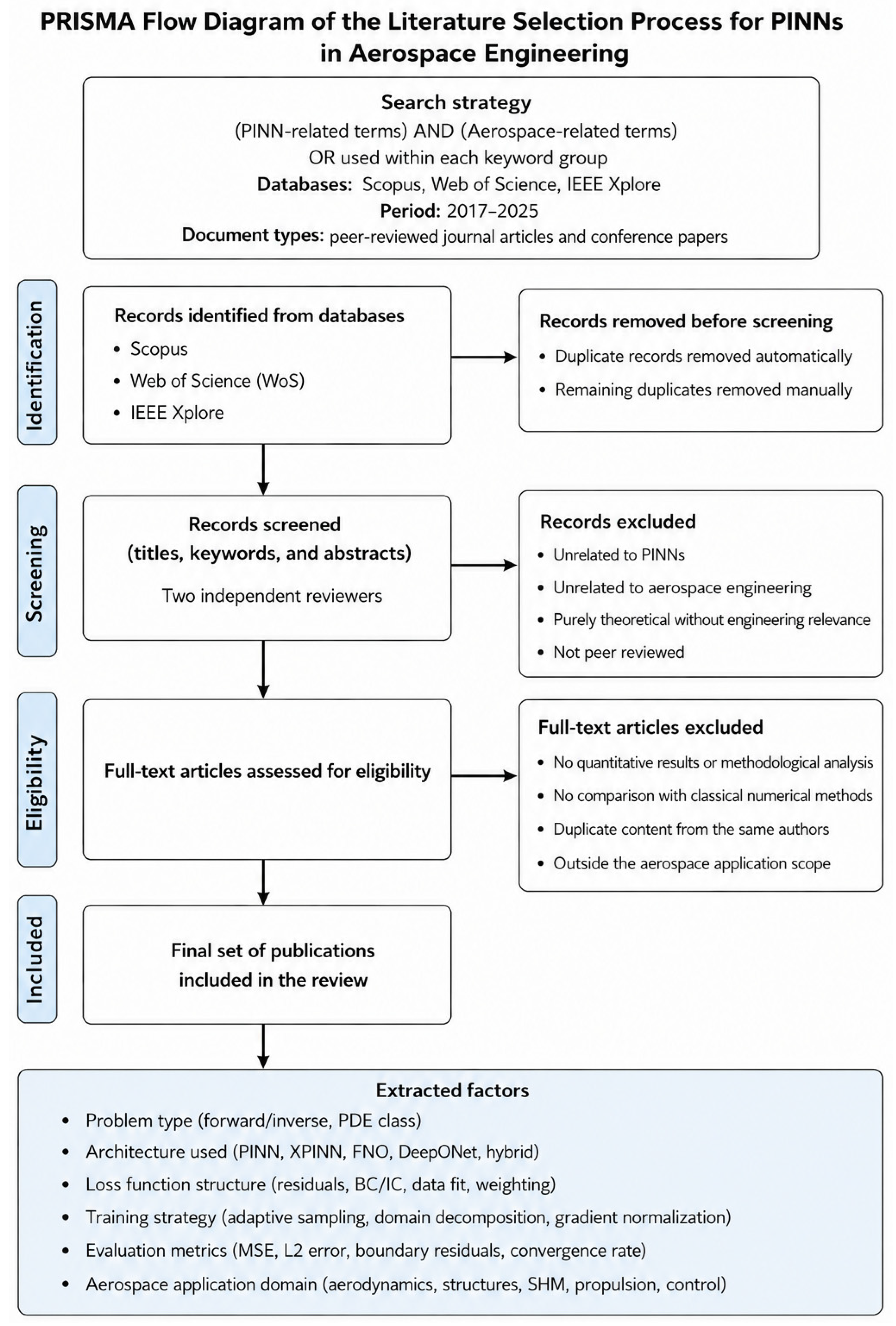
Figure 1. PRISMA scheme used in finding publications.
Applsci 16 06282 g001
Figure 2. Schematic architecture of a physics-informed neural network (PINN).
Applsci 16 06282 g002
Figure 3. Composite loss formulation scheme.
Applsci 16 06282 g003
Figure 4. Multiscale PINN framework for forward and inverse aerodynamic modeling.
Applsci 16 06282 g004
Figure 5. Domain-decomposed PINN framework with parallel local networks.
Applsci 16 06282 g005
Figure 6. Multiscale PINN architecture for coupled coarse–fine flow modeling.
Applsci 16 06282 g006
Figure 7. Comparison of PINN, hybrid PINN–CFD and data-driven aerodynamic modeling approaches.
Applsci 16 06282 g007
Table 1. Comparative performance of PINN variants and deep learning models across benchmark fluid–structure problems.
ReferenceArchitectureTraining ParametersError Metrics
[14]Baseline PINN (8 × 20)455 s (15.61 ms/epoch)Rel. L2: 0.1628
[14]NVIDIA Modulus (6 × 512)632 s (31.60 ms/epoch)Rel. L2: 0.08931
[14]DGM (6 × 512)2670 s (89 ms/epoch)Rel. L2: 0.06376
[3]Full Pipeline (FF + RWF + GradNorm + Causal)16.26 minRel. L2: 5.84 × 10 − 4
[3]Conventional PINN12.93 minRel. L2: 0.517
[3]No Fourier Features13.20 minRel. L2: 0.435
[15]a-PINN (4 layers: 64-20-20-20)28.3 minTraining loss > 0.01
Velocity MSE > 0.01
[15]can-PINN (same architecture)29.2 minVelocity MSE ~ 2 × 10 − 4
[10]Traditional PINNs5000–10,000 epochsDisplacement RMSE: 1.35–2.36%
[10]Hybrid PINN (ELM)0.9 s/iter (~40× faster)Displacement error: 7.2 × 10 − 3
[10]Optimal PINN~180 s (12× faster)Stress error < 0.1%
[12]Vanilla PINN386 sMean L2RE: 1.45 × 10 − 2
[12]hp-VPINN290 sMean L2RE: 1.43 × 10 − 2
[12]gPINN1500 sMean L2RE: 2.16 × 10 − 1
Table 2. Comparison of loss formulations, architectures, and weighting strategies in PINN frameworks.
ReferenceLoss Function ComponentsArchitectureActivation LayerWeighting Strategy
[39]Residuals of Navier–Stokes (momentum + mass) + BCs4 × 64TanhManual/static weights (Glorot init)
[35]L = λf LPDE + λb LBC + λd LData6 × 30Tanh, Swish, Sigmoid (ReLU/ELU unsuitable)Hyperparameter analysis of λ
[14]Integral formulation of LPDE, LBC, LIC1, 5, 10, 15, 20 layers; ~500 neuronsTanh, Sine, GELU, SiLUManual tuning to reach Rel. L2 < 10%
[40]Lphysical + Lboundary8 × 20TanhWeighted balancing to accelerate convergence
[41]λdata Ldata + λode Lode + λic Lic3 × 25Sine (best), Tanh, SigmoidManual balancing to keep losses same order
[31]Soft attention: point-wise weights m(λi) × residuals24–8 layer FCNNTanhSelf-adaptive weights (gradient ascent)
[42]LAN subnetworks for PDE, IC, BCMain network + LAN subnetworksTanhAdversarial weighting via gradient ascent
Table 3. Architectural characteristics and loss formulations across representative PINN variants.
ReferencePINN VariantHidden LayersNeurons ActivationLoss Type
[48]Vanilla PINN2–910–200tanhMSE (L2)
[15]CAN-PINN420–64sineCoupled AD/Numerical
[49]SPINN4 (sub-nets)64 (feature size 32)tanhSeparable Residual
[50]Steady-state NS860tanhMSE (L2)
[40]RANS Solver820tanh (best)Summed Residuals
[51]HJB Solver44096tanhL-infinity (Adversarial)
[12]PINNacle Benchmark5100tanhMulti-objective Weighted
Table 4. Performance sensitivity of PINN architectures across diverse physical problems.
ReferencePhysical ProblemLayers × NeuronsTraining Time/EpochsLoss/Error Value
[35]1D Poisson Equation2 × 20 13 s/10,000 itersMean Error: 0.0001
[35]1D Poisson Equation20 × 100 147.95 s/10,000 itersMean Error: 0.0183
[35]Volterra IDE6 × 50663.80 sMean Error:
8.91 × 10 − 4
[40]Periodic Hill (RANS)8 × 201000 Adam + L-BFGSL2 Error: 2.77%
[40]Periodic Hill (RANS)10 × 1001000 Adam + L-BFGSL2 Error: 3.78%
[21]1D Infinite Potential Well (n = 5)1 × 10010,000 epochsL2 Error:
2.02 × 10 − 5
[21]1D Infinite Potential Well (n = 5)4 × 10010,000 epochsL2 Error:
8.64 × 10 − 9
[65]Electrohydrodynamics (EHD)1 × 1625,000 epochsL2 Error: 0.00103
[65]Electrohydrodynamics (EHD)2 × 1625,000 epochsL2 Error: 0.000727
[25]3D Heat Conduction6 × 512 (Baseline)632 s/20,000 epochsRel. L2: 0.08931
[25]3D Heat Conduction6 × 512 (DGM)8174 s/20,000 epochsRel. L2: 0.07213
[41]RLC Circuit1 × 105.17 s/1,000,000 itersL2 Error: 1.12 (failure)
[41]RLC Circuit3 × 25114.7 s/1,000,000 itersL2 Error: 0.0012
[39]2D Steady Navier–Stokes4 × 6410,177.5 s (Adam) + 37.15 s (L-BFGS)Rel. L2 (u): 8.61%
Table 5. Key PINN variants, core mechanisms, advantages, and limitations.
ReferenceTypeCore DifferenceKey AdvantageKey Limitation
[48]Vanilla PINNUses a standard MLP where PDEs are imposed as soft penalty terms in the loss functionSimple to implement; mesh-free; applicable to many forward and inverse problemsSensitive to loss imbalance, spectral bias, and struggles with multiscale solutions
[45]XPINNSpace–time domain decomposition with separate networks for each subdomainHighly parallelizable; handles complex geometries; subdomains may use different architecturesMatching conditions at interfaces are complex and may cause instabilities
[62]cPINNDomain decomposition enforcing flux continuity across interfacesEnsures physical consistency; efficient for nonlinear conservation lawsMainly applicable to conservation-law problems; specialized interface conditions
[49]SPINNSeparates the network into coordinate-wise subnetworks; uses forward-mode ADDrastically reduces computational cost; enables >107 collocation points on a single GPURequires factorizable (lattice-like) collocation grids
[67]gPINNAdds gradients of the PDE residual directly to the lossHigher accuracy and improved convergenceIncreased computational cost; additional hyperparameters
[31]SA-PINNIntroduces trainable point-wise weights acting as soft attention masksAutomatically emphasizes difficult regions (e.g., sharp gradients)More parameters; more complex optimization
[68]hp-VPINNSolves PDEs in weak form using high-order polynomial test spacesExcellent for non-smooth solutions; reduces derivative order requirementsRequires numerical quadrature; accuracy depends on test space selection
[69]PIKANReplaces MLPs with Kolmogorov-Arnold Networks (KANs) using trainable activation functionsPotentially more accurate and parameter-efficient; robust to noiseNew architecture with limited theoretical grounding in PIML
[70]LPINNTwo-branch architecture solving characteristic curves and state variables separatelySmoother loss landscape; stable for high-convection regimesRequires interpolation from Lagrangian to Eulerian frame
[71]MultiInNet PINNMulti-input residual network allowing deeper layers to receive boundary/initial infoFaster convergence; fewer parameters than standard FCNNsRequires multi-stage training for best performance
Table 6. Performance and training strategies summary.
ReferenceQuantitative ResultsLoss FunctionNumber of EpochsNetwork Architecture
[16]Deflection CV: 4.25%
Bending moments CV: ≈16%
Loss drops from 1 → 0.001
Sample points: 800 interior, 400 boundary
L = α f MSE f + α w MSE w + α m MSE m + α d MSE d 1500 epochs; up to 50,000 (early stopping at 20,000–30,000)4 hidden layers × 64 neurons, tanh
[79]Relative MSE: Pressure 0.22%, Axial 0.79%, Vertical 2.39%
Total loss: O (10−4)
Data: 2000 labeled, 20,000 residuals
Multi-component RANS loss + Dirichlet BCs + periodic BCs40,000 epochs (warmup + cosine decay)9-layer FCNN, variable width
[43]Physics info improves: MSE 18%, MAE 11%, MAPE 70%, MSR 99%
Optimal ratio: γ ϕ / γ data = 2.5
Training cost: 10–100× higher than data-only
L = w 1 L data + w 2 L PDE with adaptive balancingUp to 2500 epochs (patience 200)“Wide”: 4 × 100; “Deep”: 8 × 40, Xavier init
[55]U-Net with 7.7M parameters
Dataset: 26,732 RANS solutions
Resolution: 128 × 128 × 3
L1 loss vs. OpenFOAM targets80,000 iterations (Adam, batch 10)U-Net encoder–decoder with 7 strided conv blocks + skip connections
[12]L2RE: Burgers-1D 0.00145, Poisson-2D 0.00364, NS-2D 0.0047
Vanilla PINN succeeds on 10/22 tasks
Imbalance-weighted PDE + BC + optional data loss20,000 epochs (standardized)5-layer MLP × 100 neurons
[80]MARE: O(10−2) (error < 0.5°)
Input: 150 × 150 × 1 SDF
Training: 85% of 252 RANS cases
Cost = 0.9 MSE + 0.1 GS + 10 − 5 L 2 Not explicitly statedCNN with Conv2D (300 filters, 5 × 5 & 3 × 3) + DeConv2D
Table 7. Applications of specialized PINN variants across modern aviation flow problems.
ReferenceAviation Problem SolvedType of PINN Used
[81]Subsonic inviscid flow around airfoils; forward simulation and inverse shape designNNfoil—PINN with mesh transformation to computational space
[40]Turbulent boundary layer on suction side of NACA4412 at Re = 200,000Model-free RANS-PINN—solves incompressible RANS without turbulence model
[73]Turbulent flow over NACA 2412 airfoilRANS-PINN with k–ε model—integrates 2-equation eddy viscosity model
[82]Flow around T106C turbine blade (wake, separation, transition)Viscous Compressible PINN—unclosed RANS; infers Reynolds stresses and heat flux
[79]Flow reconstruction in 2D subsonic compressor cascadeAdaptive Weight PINN—dynamic loss weighting + adaptive learning rate
[52]Combustion dynamics in rocket engine chambersMultiphysics PINN—mass, momentum, energy, species transport
[54]Transonic flow around cylinder at high Reynolds numbers (shock waves, thin BL)PINN–RANS & PINN–Euler—gradient weighting + SDF sampling
[83]Unsteady flow with moving boundaries (flapping wings, plunging airfoils)MB-PINN (Moving Boundary-aware)—immersed boundary + sequential time decomposition
Table 8. Summary of representative PINN architectures and performance metrics in aerodynamic and thermofluidic applications.
ReferenceApplicationNetwork ArchitectureTraining (Epochs/Iterations)Loss FunctionKey Quantitative Results
[91]Aerodynamic surrogate modeling for UAVs (Laplace + boundary layer equations)3 hidden layers × 12 neurons, Identity activation~2500 BFGS iterationsWeighted L2 residuals of PDE + BCsLoss < 10 − 5 ; grid dx = 0.05, dy = 0.001; absolute error < 0.0006
[50]Drag estimation for circular/elliptical particles (steady 2D NS)8 hidden layers × 60 neurons (26,105 DOF)10,000 Adam + ~140,000 total (Adam → L-BFGS)L2 residuals of mass, momentum, BCsDrag error < 6%; 100,000 sample points; inference 0.07 s vs. 120 s CFD; training 1.5 h GPU
[92]Integrated thermofluid systems (Brayton cycle, heat exchangers)Standard MLP, Xavier initialization400 Adam + TNC refinementNondimensional mass, energy, momentum residualsSolution time 0.0033 s vs. 0.2904 s; 88× speed-up; 10 LHS samples
[93]3D wake flow behind a cylinder8 hidden layers × 200 neurons, Sin activation150 epochs (Adam, LR decay 10 − 3 → 10 − 4 )L = Ldata + LPDE (NS residuals)3 × 10⁶ residual points; u-velocity error ≈ 1%; pressure error 4–5%; batch size 10,000
[15]Fluid dynamics in irregular channels3 hidden layers (128-30-30-30), sinusoidal mappingUp to 500,000 iterationsCoupled AD + numerical differentiation (CAN)Geometry: 674 boundary + 2763 interior points; training 77.3 min vs. 82.9 min (AD-PINN); MSE decreases by ×10
[10]SHM & acoustic emission localization in anisotropic compositesMulti-fidelity PINN (transfer learning LF → HF)50,000 LF + 10,000 HF epochsMulti-objective physics + mechanical response lossLocalization error 0.5075 cm (95% reduction); 98% stress accuracy; 40% cost reduction vs. FEM
Table 9. Overview of PINN variants applied to aerospace problems.
ReferenceAerospace Problem SolvedType of PINN Used
[91]Aerodynamic surrogate modeling for UAVs (Laplace + boundary layer equations)Physics-informed deep learning (PIDL/PINN)
[94]Thermochemical evolution & autoclave curing of aerospace carbon-fiber compositesDisjointed PINN
[95]Orbital state estimation & unmodeled thrust prediction for GEO satellitesKnowledge-informed PINN (astrodynamics + DNN)
[62]Inverse problems in supersonic flows (expansion waves, oblique shocks, bow shocks)XPINN (domain decomposition)
[76]Structural mechanics of helicopter blade (cantilever beam under triangular load)Fourth-order PINN
[10]Acoustic emission source localization & SHM in anisotropic CFRP panelsMulti-fidelity PINN (mfPINN)
[10]Fatigue delamination growth in composite laminates (fiber-bridging effects)Theory-constrained PINN
Disclaimer/Publisher’s Note: The statements, opinions and data contained in all publications are solely those of the individual author(s) and contributor(s) and not of MDPI and/or the editor(s). MDPI and/or the editor(s) disclaim responsibility for any injury to people or property resulting from any ideas, methods, instructions or products referred to in the content.