


Abstract
In this paper, the dynamic modeling of the anisotropic non-ideal weakly gyroscopic rotor system is considered. Equations of nonstationary transitions are derived from motion differential equations; then, the control equation, stationary frequency dependencies, and force and energy relations are obtained. When the rigidity of the elastic support is anisotropic in orthogonal directions, two critical velocities and, accordingly, two resonance regions are found. Because of the strong interaction of the rotor system with a non-ideal DC motor, slopes of the resonance curves are observed in the regions of critical speeds even in the absence of a nonlinear component of the reference stiffness, and loops are also recorded. It is proven that, compared with linear damping, the cubic nonlinearity of damping strongly suppresses the resonant amplitudes of the rotor, reduces the size of the loops even more, and strongly attenuates the Sommerfeld effects until they are completely eliminated. It is shown that an increase in the magnitude of the cubic nonlinearity of damping greatly facilitates the passage of the resonance region and expands the range of operating speeds. This proves that the amplification of linear damping with cubic nonlinearity is an effective method for controlling resonant passages and an effective damping model.
1. Introduction
Any real drive can only deliver a limited amount of power [1]. If the power of the energy source (electric motor) is not enough to overcome the resonance, the rotor speed can hang in various regions of structural resonance. Continuous operation while the system is in resonance can lead to alarmingly high levels of vibration and damage to the rotor bearings or, in extreme cases, to a general failure of the system [2,3,4,5,6]. This is known as velocity capture or resonance capture. However, when the power supply is increased to a certain limit, the captured speed almost instantly jumps to a much higher value. The speed jump is also accompanied by a corresponding drop in vibration amplitudes. This “jump” implies a sudden exit from resonance. In the literature, this phenomenon, with all its manifestations, is recognized as the Sommerfeld effect, which arises due to the internal energy coupling between the drive and the driven system, and is an important design consideration in the development of various rotating machines with flexible supports (bearings) [2,3,4,7]. An extended overview of the appearance of the Sommerfeld effect and saturation phenomenon in non-ideal vibrating systems (NISs) in macro-scales and MEMS scales is given in [8].
As a result of analyzing the dynamics of rotor systems supported by fluid film bearings (idealized as anisotropic flexible bearings), it was found that assuming rigid bearings for such systems can lead to a huge inaccuracy in the calculations of critical speeds [9]. On the other hand, some other notable work has shown that the use of flexible supports (instead of rigid supports) can actually improve the stability characteristics of rotor systems [10,11,12,13].
Most industrial rotor systems operate in the supercritical speed range. Consequently, the ability to safely traverse resonance regions constitutes one of the key requirements for reliable rotor operation. Under such conditions, the interaction between the rotor dynamics and a limited-power energy source becomes critically important. Unlike ideal drives, non-ideal energy sources actively interact with the mechanical system, giving rise to resonance capture, speed saturation, energy redistribution, and the well-known Sommerfeld effect.
Early investigations focused primarily on the classical Sommerfeld effect associated with resonance capture at critical rotor speeds. In this context, Bharti et al. [14] demonstrated that, in rigid rotor systems supported by anisotropic bearings, resonance capture may occur not only at the forward critical speed but also at the backward critical speed. The study revealed that the severity of the Sommerfeld effect depends strongly on the degree of support anisotropy and on the separation between forward and backward critical speeds. When the two critical speeds are sufficiently separated, resonance capture at the backward critical speed is relatively weak. However, as the critical speeds approach each other, both resonance zones become equally significant, and escape from one resonance may lead directly to capture at another resonance.
A more detailed characterization of this phenomenon was subsequently provided by Bisoi et al. [15], who quantified the influence of support anisotropy on the duration and extent of resonance capture. Their results demonstrated that anisotropic support properties fundamentally alter the energy exchange between the motor and the rotor system, thereby affecting the conditions under which the Sommerfeld effect occurs.
As research progressed, attention shifted from rigid isotropic systems toward more realistic rotor models incorporating structural nonlinearities, gyroscopic effects, and material anisotropy. Kafi and Hosseini [16] investigated the transient dynamics of nonlinear composite rotating shafts excited by a non-ideal energy source. Using Hamilton’s principle and the method of multiple scales, they demonstrated that eccentricity, external damping, fiber orientation, nonlinear coupling, and anisotropic material properties significantly affect both the onset of resonance capture and the resulting vibration amplitudes. Their work highlighted the importance of considering coupled bending–torsional–rotational dynamics when analyzing non-ideal rotor systems.
Further developments revealed that resonance capture is not limited to classical critical speed resonances. Bharti et al. [17] demonstrated that non-ideal rotor systems with anisotropic supports and asymmetric shaft stiffness may experience capture within regions of parametric instability. This phenomenon was termed the Sommerfeld effect of the second kind. In contrast to the classical Sommerfeld effect, which is associated with critical speed resonances, the second-kind Sommerfeld effect arises from whirl instabilities and parametric excitation mechanisms. In both cases, the excess motor power is consumed primarily by increasing vibration amplitudes rather than accelerating the rotor.
The distinction between these mechanisms was subsequently formalized by Samantaray [18], who proposed a comprehensive classification consisting of three types of the Sommerfeld effect in rotor dynamics. According to this framework, resonance capture may occur at critical speeds, within regions of parametric instability, or through combined interactions involving multiple nonlinear dynamic mechanisms. This classification provides a unified interpretation of a wide range of nonlinear phenomena observed in rotor systems driven by limited-power sources.
Another important direction of research concerns the influence of drivetrain flexibility and torsional oscillations on resonance capture. Bharti and Samantaray [19] demonstrated that torsional vibrations in a double Cardan joint driveline can substantially modify the energy-transfer process between the motor and the rotor. As a consequence, additional resonance capture regimes may arise, limiting the ability of the rotor to pass safely through critical speeds.
The growing understanding of the Sommerfeld effect has naturally led to the development of mitigation strategies aimed at ensuring safe resonance passage. Jha and Dasgupta [20] investigated the attenuation of the Sommerfeld effect in an internally damped shaft–disk system using active magnetic bearings. Their analysis showed that increasing the magnetic bias current reduces vibration amplitudes and progressively weakens resonance capture. Under certain operating conditions, the Sommerfeld effect can be eliminated entirely, enabling smooth acceleration through resonance.
A complementary control-oriented approach was proposed by Dasgupta [21], who examined non-ideal rotor systems incorporating time-delayed feedback. Through bifurcation analysis, it was shown that appropriately designed feedback control can significantly reduce instability regions, suppress vibration amplitudes, and mitigate resonance capture. These results demonstrated the feasibility of actively controlling the interaction between the motor and the rotor system.
More recently, Sinha and Samantaray [22] extended the analysis to geared rotor driveline systems. Their study demonstrated that the drivetrain configuration and transmission parameters strongly influence both the initiation and termination of resonance capture. The authors further showed that properly selected system parameters can facilitate escape from parametric-instability regions and enable successful transition to supercritical operating conditions.
The most recent developments have emphasized the crucial role of damping mechanisms in determining the occurrence and severity of the Sommerfeld effect. Movahedi et al. [23] investigated a rotating shaft modeled using Timoshenko beam theory and incorporating both internal and external damping. Their results demonstrated that damping not only affects vibration amplitudes but also significantly alters the conditions for resonance capture and resonance escape. In contrast to classical Euler–Bernoulli models, the inclusion of shear deformation and rotary inertia provided a more realistic representation of high-speed rotor dynamics and highlighted the importance of accurately modeling energy-dissipation processes.
Overall, the evolution of research on rotor systems driven by non-ideal energy sources demonstrates a gradual progression from relatively simple isotropic rotor models exhibiting the classical Sommerfeld effect toward increasingly complex systems involving anisotropic supports, gyroscopic effects, nonlinear coupling, parametric instabilities, drivetrain flexibility, and sophisticated damping mechanisms. Despite significant advances, the combined influence of anisotropic stiffness, linear damping, nonlinear damping, and non-ideal energy sources on safe resonance passage remains insufficiently understood. In particular, reliable methodologies for identifying damping mechanisms and predicting resonance transitions in anisotropic rotor systems continue to represent an important open problem in modern rotor dynamics.
In recent years, growing attention has been devoted to the application of nonlinear approaches in the design of vibration-isolation and vibration-control systems. Studies [24,25,26,27] have demonstrated that cubic nonlinear damping can not only reduce vibration amplitudes in the resonance region but also improve the vibration-isolation performance of a system in the super-resonant operating range. Furthermore, it has been established that the introduction of nonlinear damping may significantly attenuate the manifestations of the Sommerfeld effect, including the associated jump phenomena, and can even lead to the complete elimination of resonance capture. These findings indicate the high potential of nonlinear energy-dissipation mechanisms as an effective means of controlling the dynamic behavior of rotor systems driven by non-ideal energy sources.
Recent studies have shown that nonlinear damping is an intrinsic property of many viscoelastic materials and structural components operating under large-amplitude vibrations. Balasubramanian et al. [28] experimentally investigated the viscoelastic response and nonlinear damping of rubber plates and demonstrated that energy dissipation strongly depends on vibration amplitude. Amabili [29] established that nonlinear damping may significantly exceed linear damping in large-amplitude vibration regimes and proposed a physically based derivation of nonlinear damping from viscoelastic constitutive laws. Further developments by Amabili et al. [30] extended these concepts to fractional viscoelastic structures and demonstrated the important role of nonlinear damping in determining the dynamic response of flexible systems. A comprehensive review of nonlinear damping identification methods was subsequently presented by Al-Hababi et al. [31], who summarized the current State of the Art, existing challenges, and future research directions in nonlinear parameter identification. These studies demonstrate that accurate identification of nonlinear damping and stiffness characteristics is a prerequisite for the practical implementation of advanced vibration-control strategies and safe resonance-passage techniques.
However, the practical implementation of such approaches requires reliable identification of the nonlinear stiffness and damping parameters characterizing real supporting structures and materials. Consequently, in recent years, considerable research efforts have been focused on the development of methods for identifying nonlinear parameters of mechanical systems that are non-ideal factors [32]. Of particular interest has been the independent determination of nonlinear stiffness coefficients, linear viscous damping coefficients, and nonlinear damping coefficients from experimental amplitude–frequency and time-domain responses. The evolution of identification techniques has followed a consistent progression: from the estimation of nonlinear stiffness parameters alone to the simultaneous identification of stiffness and damping characteristics, and subsequently to the determination of nonlinear and asymmetric energy-dissipation properties.
One of the simplest classes of identification problems concerns the estimation of nonlinear stiffness parameters. Lu et al. [33] proposed a method for identifying nonlinear stiffness and damping parameters based on the jump frequencies and jump amplitudes observed in nonlinear frequency-response curves. The authors demonstrated that the incorporation of both jump frequencies and the corresponding jump amplitudes significantly improves the accuracy of nonlinear parameter estimation.
Further developments in identification methodologies have focused on the simultaneous estimation of nonlinear stiffness and linear damping. Civera et al. [34] proposed a generalized power-law formulation for stiffness and damping nonlinearities, enabling the description of a broad class of nonlinear systems through parameters directly identified from experimental data. Compared with conventional polynomial models, this approach substantially enhances the flexibility and applicability of nonlinear dynamic modeling.
Significant progress has been achieved in the identification of nonlinear stiffness, linear damping, and cubic nonlinear damping. Le Guisquet and Amabili [35] developed an identification procedure for geometric nonlinear stiffness and cubic nonlinear damping based on the harmonic balance method combined with genetic algorithms. The methodology is applicable to both hardening and softening nonlinear systems and has been successfully validated using experimental data.
A separate line of research is devoted to the identification of asymmetric nonlinear damping characteristics. Chatterjee and Chintha [36] proposed an identification and parameter-estimation methodology for asymmetric damping nonlinearities based on higher-order frequency response functions and Volterra series representations. The method enables the separation and quantification of quadratic and cubic-damping contributions and allows for the simultaneous estimation of both linear and nonlinear damping parameters from experimentally measured dynamic responses. The proposed approach demonstrated good accuracy in identifying asymmetric energy-dissipation mechanisms in nonlinear vibrating systems.
A direct identification methodology for nonlinear damping was introduced by Lisitano and Bonisoli [37]. Unlike equivalent-linearization approaches, the resulting nonlinear model remains valid over a wide operating range and allows for accurate prediction of the system response under various excitation levels.
Another important research direction concerns the identification of asymmetric nonlinear damping characteristics. Chatterjee and Chintha [38] developed an identification algorithm for asymmetric nonlinear damping represented by polynomial functions containing quadratic and cubic nonlinear terms. The proposed method is based on higher-order frequency-response functions derived from Volterra series and enables the simultaneous estimation of both linear and nonlinear damping parameters.
A comparative analysis of existing nonlinear parameter-identification techniques was performed by Wang et al. [39]. The authors demonstrated that separating the effects of nonlinear stiffness and damping remains one of the most challenging problems in nonlinear system identification, particularly in systems exhibiting asymmetric characteristics.
Recent research has increasingly focused on advanced signal-processing techniques and artificial intelligence-based approaches. Safari et al. [40] proposed a data-driven structural identification framework for nonlinear systems exhibiting asymmetric stiffness and damping nonlinearities. Furthermore, Das et al. [41] developed a frequency-domain identification method for fractional-order Duffing systems, enabling the estimation of mass, linear damping, linear stiffness, and nonlinear stiffness parameters from experimentally measured frequency-response functions. The proposed methodology provides an efficient framework for identifying nonlinear dynamic systems with memory-dependent behavior and fractional-order characteristics.
Additional advances have been achieved in the experimental identification of nonlinear damping through restoring-force reconstruction techniques. Additional progress in nonlinear system identification has been achieved through restoring-force-based methodologies. Rogers and Friis [42] proposed a latent restoring force approach that combines Bayesian filtering, Gaussian process modeling, and state-space representations. Unlike conventional Restoring Force Surface techniques, the method treats the nonlinear restoring force as a latent variable and estimates it directly from measured dynamic responses. The approach enables simultaneous reconstruction of system states and nonlinear forces while accounting for measurement uncertainty and was successfully validated using both numerical and experimental benchmark systems. Diala et al. [26] demonstrated that cubic nonlinear damping has a significant influence on the dynamic behavior of nonlinear systems in the vicinity of resonance and therefore must be considered when developing identification models.
Overall, the reviewed studies demonstrate a clear evolution from the identification of nonlinear stiffness alone toward the independent determination of nonlinear stiffness, linear damping, cubic nonlinear damping, and asymmetric nonlinear characteristics. Nevertheless, studies devoted to the independent identification of these parameters in the anisotropic viscoelastic supports of rotor systems remain relatively scarce. In particular, reliable methodologies capable of independently determining nonlinear stiffness coefficients, linear viscous damping coefficients, and pure cubic nonlinear damping coefficients from experimentally measured frequency-response characteristics are still largely unavailable. Therefore, the development of such identification methods represents a scientifically significant and practically relevant research direction.
The analytical–numerical methodology proposed in this study contributes to this field by enabling the independent determination of nonlinear stiffness coefficients, linear viscous damping coefficients, and pure cubic nonlinear damping coefficients of support materials employed in weakly gyroscopic rigid rotor systems [43]. The proposed identification procedure is based on stationary vibration amplitudes obtained from harmonically excited rotor systems and provides a physically meaningful framework for parameter estimation in anisotropic viscoelastic supports.
2. Materials and Methods
2.1. Equations of Motion
A non-ideal weakly gyroscopic rotor–DC motor system is considered (Figure 1). The rotor consists of a disk, a shaft, and a support device. The disk has the mass, ; moment of inertia about its polar axis, ; and moment of inertia about its diametrical axis, , and it is fixed without skewness at the free end of the rigid shaft. The shaft without mass with the length is installed vertically with the help of the lower hinge and the upper elastic support spaced from it at the distance . With such a location of the disk on the shaft relative to the supports and at a sufficiently high speed of shaft rotation (), the system can be considered as a gyroscopic rotor. In a fixed coordinate system, , the position of the geometric center of the disk, , determines the coordinates , and the spatial position of the shaft determines the angles, and , and the angle of rotation, . We take the coordinate as equal to and exclude it from consideration. Next, we denote the coordinates of the center of mass, , of the disk through and . We also assume that the linear eccentricity, , is directed along the N axis of the ONKZ coordinate system. In the case of small deviations of the rotor axis, .
Figure 1.
Rotor geometry.
Considering the foregoing information, the projections of the angular velocity on the coordinate axes of the ONKZ system can be written as
The relationship between the coordinates and , and and is expressed by the following relations:
Thus, the position of the rigid shaft and the rotor as a whole in space is determined by the angles , and .
It is convenient to represent the equations of motion of the rotor in the form of the Lagrange equations of the second kind. To do this, we first compose an expression for the kinetic energy of the disk in accordance with Koenig’s theorem [44]:
Assuming that and using (1) and the relationship (2) between the coordinates and , and and , the expression for the kinetic energy of the rotor is presented in the final form of
The projections of the moment of gravitational force have the form
where is the disk weight.
As is known, the resonant properties of nonlinear oscillatory systems depend very much on the properties of the energy source [1]. In [44,45], it was assumed that the torque of an engine used in a non-ideal oscillatory system is proportional to the rotational speed of its shaft.
The dynamic moment of the motor, in accordance with [1,46], has the following expression in general form:
where is the motor torque (motor characteristic), and is the moment of resistance force to the rotation of the motor rotor.
In [47,48], the possibility and expediency of using static characteristics of energy sources in the equations of motion, as well as the acceptability of restrictions and assumptions used in the analysis of these equations, were experimentally confirmed. Then, in accordance with [47,48], substituting the found value, , into (5), we obtain an expression for the dynamic moment of an electric motor with a permanent magnet in the form
where is the magnetic flux of one pole; is the angular velocity of rotation of the armature; is the voltage applied to the electrical circuit of the motor; is the resistance of the entire power circuit; the electrical constant, , and mechanical constant, , are equal to each other; and is the coefficient of resistance to rotation of the motor rotor.
The upper bearing support of the gyroscopic rotor can be made of nonlinear viscoelastic materials such as natural rubber, rubber, and other polymers widely used as vibration dampers. As is known, rubber shock absorbers, in addition to linear viscoelastic properties, have both nonlinearity of damping and nonlinear stiffness [49,50].
There are various nonlinear damping models. The phenomenological model of nonlinear damping is added to the equations of motion in the studies [24,25,26,27,51,52,53] and others. It considers two types of n-th damping terms: the first type is represented by the velocity multiplied by the (n − 1)-th power of the displacement, and the second type is proportional to the n-th degree of velocity [24,25,26,49]. The mechanism of nonlinearity of damping was modeled by the scattering of thermally excited vibrational modes from the assumed eigenmode in [54].
In accordance with the second damping type, the moments of the dissipative forces with linear and cubic nonlinear components acting in the flexible support can be described by the Rayleigh function, in its more general form:
where are coefficients of linear viscous damping, and are coefficients of cubic nonlinearity of damping in mutually perpendicular directions. These coefficients have different dimensions and may differ in values.
The studies in [55,56] are very informative. Experiments showed a strong increase in damping with oscillation amplitude for nonlinear oscillations of beams, plates, and shells. Nonlinear damping was determined in this research by viscoelasticity using a single-degree-of-freedom model derived from a standard linear solid material that includes geometric nonlinearity. The developed damping model is represented by the product of the velocity and the square of the displacement, and its parameters were determined experimentally. The results of the study of forced vibration responses measured for a rectangular plate with a free edge are interesting in that they represent a case where energy does not pass through the boundary.
If we take into account that the rotor shaft is rigid, only its upper support has anisotropic elasticity, and the elastic forces in mutually perpendicular coordinate directions are, respectively, equal to and , then the potential energy of the system can be represented as
where are coefficients of linear rigidity, and are coefficients of nonlinear rigidity of the support in mutually perpendicular directions.
We represent the Lagrange equations of the second kind for the rotor system as follows:
Here, the generalized coordinates are represented by the angular coordinates , and the generalized forces are represented by projections of the moment of gravity () and dynamic torque of the motor (), defined by Formulas (4) and (6).
We substitute Expressions (3), (4), and (6)–(8) into (9), and we discard the perturbations containing (since, in the region close to the resonant velocity, << ), perturbations with the parameter (since, in what follows, we assume that << ), quantities of the second and higher orders of smallness with respect to the angular coordinates ( and ), their derivatives, and their combinations. We thus obtain the equations of motion of the rotor:
On the right part of the obtained equation system in (10), the components of the projections of the moment of gravity are also neglected, since >> for a fast-rotating rotor.
The theoretical justification of the accepted assumptions, as well as an assessment of the legality of neglecting individual terms in the derivation of the system of equations of motion (10), is given in Appendix A.
Below are the natural frequencies (critical speeds) of the dampened rotor system (10):
where
In this case, >> :, .
For numerical calculations using Formulas (11) and (12), some geometric and dynamic parameters of the weakly gyroscopic rotor system are borrowed from the experimental setup used in [25]: l1 = 0.46 m, l2 = 0.33 m, m = 2 kg, k11 = 2 104 Nm−1, k12 = 2.4 104 Nm−1, JD = 0.090 kgm2, JP = 0.011 kgm2, and er = 0.00193 m.
Now, we can calculate the natural frequencies (critical speeds) of the gyroscopic rotor system (10): ω1 = 64.94 Hz and ω2 = 71.24 Hz.
The angular velocity of rotation of the shaft, ω1, in the interval [64.95 Hz, 64.48 Hz] can be approximately considered constant and equal to ω1 = 65 Hz. This makes it possible to use ω1 in the process of bringing the parameters into a dimensionless form.
We introduce the following dimensionless parameters:
With the use of (13), the equations of motion (10) can be represented in a dimensionless form:
where
is the dimensionless natural frequency of the rotor system in (14) at , and
is the dimensionless natural frequency of the rotor system in (14) at , where >> is accepted.
In the third equation of System (14),
is the dimensionless dynamic torque of the motor. Here, is the dimensionless normalized motor voltage (control parameter), which depends on the voltage of the motor; and is a parameter depending on the type of energy source [14,57].
Here, the prime denotes the derivative with respect to the dimensionless time, .
We are interested in the effect of the cubic nonlinearity of damping on the dynamics of a weakly nonlinear rotor system, taking into account the anisotropy of the support rigidity and the change in voltage of the motor with a characteristic taken as a straight line [14,57].
To use the Bogolyubov method [1,25,58,59,60], the following restrictions are accepted for the analytical solution of the equations of motion. The projections of the moments of linear and nonlinear damping forces, and , as well as the moment of the nonlinear elastic force, ; moments of the inertia forces, ; and passive gyroscopic moments, , are assumed to be small compared to other moments of forces acting in the system. Due to the fact that we confine ourselves to considering regimes close to stationary motions, the acceleration, , is small. We also confine ourselves to considering motion in resonance regions, where the frequencies of the free oscillations, , are close to the frequency of forced oscillations, ; that is, the values of the so-called frequency detuning () are small. In order to reflect the smallness of the detuning Δ1 and Δ2 in an explicit form, we further represent them using a dimensionless small positive parameter, ε, in the form of the relations and , where and have the same dimension as Δ1 or Δ2.
After the introduction of the small parameter, ε, in accordance with the accepted constraints of the problem and the new notation for values,
the equations in (14) will look as follows:
The equations in (19) are a system of nonlinear ordinary differential equations of the second order with respect to , and , with the small parameter, ε, for a non-ideal anisotropic gyroscopic rotor system.
2.2. Solutions of Equations of Motion
At small angular deviations of the shaft, and , harmonic oscillations at the frequency of the driving moment predominate in the solutions of System (19). Due to the anisotropy of the support rigidity in orthogonal directions, oscillations in these directions occur in different ways: with different amplitudes and different phases. Then, we define the solutions of System (19) in the following form:
Here, are the oscillation amplitudes in mutually perpendicular directions, and are the phase shift angles between the angular coordinates, and , and the disturbing moment, respectively. They represent the most essential parameters of motion and are slowly varying functions of time, .
Following the method of Bogolyubov’s theory of small perturbations [1,25,58,59,60], and taking into account (20) and (21), we obtain a system of vorticity equations equivalent to System (14), approximate solutions of which can be found in the form
where are small periodic functions of time, .
After averaging and excluding the small parameter, ε, in accordance with the formulas for converting parameter values (18), the equations for nonstationary vorticity follow from the obtained averaged equations of the first approximation [25,49] with respect to the oscillatory parameters, , of the first harmonic, depending on the dimensionless motor voltage, :
Under the conditions of the existence of stationary modes of motion,
We obtain from (23) the control equation (frequency equation) and the equations of stationary joint amplitude– and phase–frequency characteristics:
From (24) and the first and third equations of System (25), and assuming that the relations and are possible in the resonance region, we obtain the so-called control equation [25,49] in the following form:
Equation (26) is valid within the resonance region of the oscillatory system. As is known, the width of the resonance curve, Δω, determined at the level of amplitudes that are times lower than the maximum resonance amplitude, is characterized by the ratio of the dissipated power, , to the energy, , stored in the oscillatory system. According to the energy approach, the quantity ΔΩ is directly proportional to the dissipated energy and inversely proportional to the energy accumulated by the oscillatory system, and it is defined by the expression
Consequently, Equation (26) is used to derive the formulas for and .
Thus, Equation (26) characterizes the dynamic relationship between the source of limited excitation and the oscillatory system in the resonance region. It describes the process of energy redistribution between the rotational motion of the rotor and the oscillatory motion of the system. Consequently, the rotational speed is determined by not only the mechanical characteristic of the motor but also the parameters of the vibrational response of the system.
Having jointly solved the equations of System (25) numerically, we find the amplitudes, and ; initial phases, and ; and stationary oscillations. Equations (25) and (26), when the conditions ωn1 = ωn2 = ωn, μ11 = μ12 = μ1, μ31 = μ32 = μ3, and a = b are satisfied, are converted into expressions for the case of a rotor with an elastic support with isotropic reducing and damping properties [25,49].
The dependence of the oscillation frequency, , on time, , taking into account the higher harmonics, is defined as
The results of the research show that the higher harmonics of the oscillations practically do not affect the amplitudes, phases (22), and oscillograms of the deviation angles, α and β; their oscillations are practically harmonic [1,25].
2.3. Ratio of Moments and Ratios of Power and Energy
In the case of a non-ideal rotor system, the parameter should be determined as the roots of Equation (26), which correspond to the values of the amplitudes, and ; phases, and ; and oscillations in orthogonal directions, calculated according to (25). If we take into account that the characteristic of the motor is pre-selected as a straight line, then, considering Equation (26), the corresponding required dynamic moment of the motor is
Then, Equation (26) can be assumed to be an equilibrium equation for the moment of the moving forces of the energy source and the moments of vibration damping forces in the steady state. From (26), by multiplication term by term with , one can obtain the power equation:
where
is the dynamic power of the energy source (DC motor), and
is the power expended on damping the oscillatory motion.
Now, using (30), we find the energy released during a period by the electric motor:
Similarly, the energy spent over a period on damping the oscillatory motion can be represented on the basis of (31) in the form
Expression of moments (26), as an expression of powers (28), is easy to obtain from the first integrals of the equations of motion (26) according to the method described in [1,25].
3. Results and Their Analysis
3.1. Impact of Damping on Rotor Dynamics
The following values of dimensionless parameters were used for calculation operations: ; ; and . The results of numerical calculations using Formulas (25) and (26) are shown in Figure 2, Figure 3, Figure 4, Figure 5, Figure 6 and Figure 7.
Figure 2.
Shaft rotation speed depending on the dimensionless normalized motor voltage: (a) linear damping coefficient and (b) various values of linear damping coefficient.
Figure 3.
Shaft rotation speed depending on the dimensionless normalized motor voltage: (a) cubic nonlinearity of damping and (b) various values of cubic nonlinearity of damping.
Figure 4.
Stationary oscillation amplitudes of an anisotropic rotor depending on the dimensionless normalized supply voltage at various values of the coefficients: (a) linear damping and (b) cubic nonlinearity of damping.
Figure 5.
Stationary oscillation amplitudes of a rotor depending on the speed of shaft rotation at various values of the coefficients: (a) linear damping and (b) cubic nonlinearity of damping.
Figure 6.
Stationary oscillation amplitudes, a (a) and b (b), for various values of the linear damping coefficient.
Figure 7.
Stationary amplitudes, a (a) and b (b), of oscillations at various values of the coefficient of cubic nonlinearity of damping.
During rotor speedup (speed increase), the steady rotor speed follows the trajectory →a→b→g→c→d→e→, containing frequency capture at a lower threshold of stability on the paths a→b and c→d, as well as the two hopping effects b→g and d→e (Figure 2a).
During rotor slowdown (speed reduction), the steady rotor speed follows the trajectory →e→f→f→c*→g→h→a*→, containing frequency capture at lower threshold of stability in the directions c*→c and a→a*, as well as the two hopping effects, f→c* and h→a* (Figure 2a). In two perpendicular directions, the support stiffness has different values, and therefore, two different jumping effects are observed at two input voltages [60]. The hop sizes in the second critical speed region are comparatively higher than those in the first critical speed region [15]. The resonance response curve contains two unstable segments, namely the branch between points h and b and the branch between points f and d, corresponding to the shaft-speed intervals hg and fe, respectively. It should be noted that the shaft-speed values located on the h–b and f–d branches, which correspond to voltage ranges of 1.266–1.290 V and 1.400–1.468 V, respectively, are physically unattainable because these segments are dynamically unstable [43,61,62]. As a result, corresponding to the two stable branches, there are only two possible speed values near the resonance region; one of them can be accessed during speedup operation and the other during slowdown operation.
As the linear damping value increases from 0.01 to 0.02, points b and d shift to the left, and points a* and c* shift to the right. Consequently, the size of Ω hops significantly, decreases from 1 ÷ 1.036 to 1 ÷ 1.019 in the first critical speed region and from 1.1 ÷ 1.179 to 1.1 ÷ 1.141 in the second critical speed region, and the size of unstable branches also becomes smaller; the Sommerfeld effects are significantly attenuated (Figure 2b) and further increase in linear damping to the value of 0.04, completely removing the above effects (Figure 2b) [3,61].
The addition of a linear damping of the magnitude 0.01 with a cubic nonlinearity of damping of the magnitude 0.01 (Figure 3a) ensures the disappearance of the unstable branch in the region of the first critical speed, a significant reduction in the size of the jump in Ω from 1.1 ÷ 1.179 to 1.1 ÷ 1.127, and, consequently, a reduction in the unstable branch in the region of the second critical speed. When the cubic nonlinearity of the damping component is further increased to 0.02 (or to 0.04), it virtually removes the Sommerfeld effect in the second resonance region (Figure 3b).
In the structure of the resonant region, as the drive voltage increases and the critical speed approaches, the angular velocity of the shaft does not increase, and the driven energy is spent on excitation of the rotor vibration. When the driven power reaches a critical value, the vibration amplitudes sharply decrease with a simultaneous increase in the speed of rotation of the shaft. Figure 4 shows graphs of vibration amplitudes in orthogonal directions versus drive voltage for different values of the linear damping coefficient (Figure 4a) and coefficient of cubic nonlinearity of damping in the presence of a constant value of linear damping () (Figure 4b). It is easy to see from them that both sets of values, and , dampen the maximum resonant amplitudes, but there is an effect of linear damping combined with cubic nonlinearity of damping.
Gyroscopic interaction affects the stability and shape of the resonance characteristic [26]. As the value of linear damping () increases from 0.01 to 0.04 (Figure 4a), the dimensions of the loop of the resonance curve for the amplitude a in the second resonant region, and for the amplitude b in the first resonant region, decrease. Complementing linear damping of a value of 0.01 with cubic nonlinearity of damping of values of 0.01, 0.02, and 0.04 reduces the size of these loops so much that they become the peak points of the amplitude rises (Figure 4b).
For comparison, Figure 5a,b show the stationary amplitude–frequency characteristics of an ideal anisotropic gyroscopic rotor system [62]. In them, instead of the loops observed in the previous figures, there are amplitude elevations, the maximum values of which decrease as the damping value increases. So, due to the strong interaction of the rotor with a non-ideal energy source—a DC motor—the resonance curves of both directions incline toward the drive voltage axis, accompanied by Sommerfeld effects with jumps, and loops appear in them [14].
Figure 6 show three-dimensional plots of drive voltage; shaft angular velocity; and oscillation amplitudes, a and b, for different values of the linear damping coefficients. Under the influence of damping, the hook formed instead of the loop is straightened. However, in a similar graph in Figure 7a, there is a loop in the resonance curve formed by the intersection of the amplitude values, which decreases in size as the magnitude of the cubic nonlinearity of damping increases. Branched loop-curves for various values of nonlinearity of damping merge into one line as the voltage and rotation speed.
In Figure 7b, the amplitude elevation of the first resonant region under the influence of nonlinearity of damping is so suppressed that it hardly differs from the main resonant curve. Thus, the graphs in Figure 6 and Figure 7 show the overall picture of the non-ideal dynamics and the effect of linear damping and cubic nonlinearity of damping on them in the stationary mode.
Let us consider a special case when the rotor consistently gets stuck at both critical speeds. At the values and in velocity characteristics, a sequential double resonant capture with jumps is apparent; at and , effects at the boundary of the zones of two resonant captures are apparent; and at and , the Sommerfeld effect in the region of the first critical velocity is eliminated.
Figure 8 shows the calculation results according to Formulas (25) and (26) as diagrams of the rotor vortex velocity, Ω, depending on the dimensionless voltage of the engine, u1, at various damping values. According to Figure 8a, two distinct jumps are observed (one for one direction at , and the other for another direction perpendicular to the first one at ).
Figure 8.
The speed characteristic of the rotor at different values of the linear damping coefficient: (a) μ11 = μ12 = 0.004; (b) μ11 = μ12 = 0.006.
These two jumps are quite close to each other, which leads to resonance capture. The dotted lines in Figure 8a show the state of “no imbalance”. In the mode of increasing the engine voltage, the first jump occurs at point “b” (i.e., u1 = 1.280). This jump corresponds to the passage through the first resonance and should ideally position the rotational velocity at point “g*”, lying on the dotted line. However, the velocity actually jumps from “b” and subsequently stops at point “g”, since the system encounters the second resonance zone much earlier, which prevents the transition to point “g”. As soon as this happens, the rotor rotational velocity stops at the second critical velocity prior to point “d” [6], corresponding to u1 = 1.550 (i.e., the position in which the second jump occurs). After the second jump from “d” to “e”, the dependence of velocity on voltage almost follows the linear trend indicated in equation . If the resonant zones were not located one after the other, then the first jump would be quite simple (i.e., from “b” directly to “g*”). Instead, because of the back-to-back jump segments, the velocity trajectory traces from “b” to “g”, then from “d” to “e”, and finally from “e” onward.
When the linear damping value increases from 0.004 to 0.006 (see Figure 8b), the size of the jumps along Ω significantly decrease (from 1 ÷ 1.014 to 1 ÷ 1.011 in the first resonant region, and from 1.020 ÷ 1.245 to 1.020 ÷ 1.174 in the second resonant region), but the phenomenon of sequential double resonant capture remains.
A linear damping value of 0.004 enhanced with a cubic nonlinearity of damping value of 0.002 (see Figure 9a) leads to the intersection point of the nonlinear jump line with the line of dependence of shaft rotation speed on motor voltage being displaced to the boundary of regions of two resonant captures, reduction in the sizes of unstable branches in resonant curves, and significant reduction in the jump size of Ω from the range of 1–1.014 to 1–1.010 in the first resonant region, and from the range of 1.020–1.245 to 1.020–1.086 in the second resonant region.
Figure 9.
The speed characteristic of the rotor at different values of the coefficient of cubic nonlinearity of damping; (a) μ11 = μ12 = 0.004, μ31 = μ32 = 0.002; (b) μ11 = μ12 = 0.004, μ31 = μ32 = 0.002, 0.004, 0.006.
A comparison with the case of linear damping with a value of 0.006 also proves the predominant effect of nonlinearity of damping on reducing the values of unstable branches and, accordingly, the jump intervals. A further increase in the magnitude of the cubic nonlinearity of damping can eliminate the Sommerfeld effect with a jump, starting from the first resonant zone (Figure 9b).
As a result of the strong interaction of the rotor system with a non-ideal energy source, loops appear in the resonant curves (Figure 10a) in areas bounded by jump lines, i.e., in bistability zones that do not exist in the ideal system (instead, there are elevations in the resonant curves). In the case of linear damping values of 0.004 and 0.006, the vertical size of the loop for the amplitude resonance curve, a = a(u1), is significantly larger than the value of the maximum resonant amplitude. The second loop is located on the back of the amplitude resonance curve. Under the influence of a cubic nonlinearity of damping magnitude of 0.002 with a constant linear damping magnitude of 0.004, the dimensions of the loops in all directions significantly decrease compared with the change in the magnitude of the maximum resonant amplitude (Figure 10b). The strong interaction of the system with the energy source affects the amplitude characteristics like the positive nonlinear cubic stiffness of an elastic support, although it does not exist, bending the resonant curve and its loop to the right side. Under the influence of damping, the effect of the interaction of the excitation source with the rotor system is suppressed, and the amplitude characteristic is straightened, decreasing in maximum dimensions.
Figure 10.
The amplitude characteristic of the rotor at different damping values: (a) μ11 = μ12 = 0.006; (b) μ11 = μ12 = 0.004, μ31 = μ32 = 0.002.
Now, let us consider the case of the presence of a nonlinear cubic component of the stiffness of an elastic support. It is known that the nonlinear stiffness of the support not only preserves vibration isolation in the resonant region, but also transfers it to an area beyond the critical velocity [44]. As a result, the shaft rotation speed will not get stuck near the critical speed, but will increase with increasing voltage (the steeper the slope is, the greater the value of nonlinear stiffness is) [49], thereby reducing the likelihood of the Sommerfeld effect. The angular velocity of the shaft reaching point b or d (Figure 2) jumps to a higher value. The curves of the amplitude characteristic stretch from the end, and the greater the slope on the stress axis is, the greater the nonlinear stiffness is. With an increase in the damping value, the sizes of jumps and unstable branches are reduced [49]; in the case of cubic nonlinearity of damping, this is more significant.
3.2. Energy Resonant Passage and Damping Effects
In the dynamics of a non-ideal anisotropic gyroscopic rigid rotor, the aim is to determine the control conditions for smooth and fast resonance escape using energies, linear damping, and cubic nonlinearity of damping. To this end, following the methodology of the works [1,14,63], graphs of dissipated energy (), as a function of shaft speed (), are first plotted according to Formula (33) at different values of linear damping ( and ) (Figure 11a) and cubic nonlinearity of damping ( and ) at constant linear damping () (Figure 11b). Near them, plots of motor energy () as a function of shaft angular speed () at different values of driven voltage () are plotted using Formula (32). The straight lines, , pass through the critical speeds, and ; through the peaks of the energy resonance curves —which correspond to the driven voltage values, and (Figure 2a and Figure 3a), at different values of linear damping and cubic nonlinearity of damping (Figure 2b and Figure 3b); and through points above the maxima of the curves, . It should be mentioned that in [61], the approach was carried out using the total power and the power dissipated in the damping.
Figure 11.
Energy depending on the speed of rotation of the shaft at different damping values: (a) μ11 = μ12 = 0.01, 0.02, 0.04; (b) μ11 = μ12 = 0.01, μ31 = μ32 = 0.01, 0.02, 0.04.
In Figure 11a, in the first critical speed region, the source energy lines, for = 1.245 and for = 1.269, intersect the dissipation energy line, , with , and these values of motor energy () are insufficient to overcome the first resonance region. Therefore, rotor speed capture occurs; that is, it is trapped in resonance for an indefinite time in both conditions. However, the straight line, , at = 1.269 for the case of is a boundary line. The energy, , at = 1.290 for the line with is limiting, but for , it becomes sufficient for a smooth transition to the resonance region. The source energy, , for = 1.312 sufficiently provides smooth crossing of the first resonance region in the case of , and it is a decent margin for passing the resonance region in other cases of Equivalently, in the case of , the energy, , with = 1.515 is sufficient for smooth passage through the region of the second resonance, while in the case of , the energy () with = 1.468 is even less.
Hence, the larger the damping value is, the smaller the energy requirements of the force to smoothly pass the resonance curve region are. In the case of , there is no Sommerfeld effect with nonlinear hops in the response of the dynamics (Figure 3). This supports the claim [2] that high damping often suppresses the Sommerfeld effect.
With a linear damping value of 0.01 supplemented with a cubic-damping nonlinearity of 0.01, the Sommerfeld effect will only occur in the region of the second resonance, while it will be absent in the region of the first resonance (Figure 11b). The energy, , at = 1.370 and = 1.405 will not be sufficient to pass the second resonance region, and that at = 1.410 is the limiting energy beyond which a smooth resonance passage can be achieved, for example, at for = 1.430.
Comparing the boundary energy of the smooth second resonance passage of the cubic nonlinearity of damping case of at (Figure 11b) with the same energy of the linear damping case at (Figure 11a), we can see that the first value of at = 1.410 is less than the second value of at = 1.421, even without considering the unobstructed energy passage through the first resonance region in the nonlinearity of damping case.
Similarly to that in the linear damping case (Figure 11a), the energy, , at = 1.405 for the curve with is a threshold, and that at = 1.410 for the curve with is a threshold, but for the case of , it is sufficient for free resonant passage.
It can therefore be argued that in the resonant regions, the larger the damping effect is, the less energy of the resonant oscillations goes to dissipation. Therefore, predominantly amplifying the cubic nonlinearity of damping is an effective model of optimal damping and an effective resonant amplitude control method for smooth passages.
3.3. Transient Response and Damping Effects
The transient differential equations in (23) were numerically integrated in the MATLAB R2025a software environment using the ode23. function. This solver implements the explicit one-step Runge–Kutta–Bogacki–Shampine method of the order 2 (or 3) with automatic selection of the integration step. The method is intended for solving non-stiff systems of ordinary differential equations. Integration was performed using the time interval . To control the accuracy of the numerical solution, the absolute and relative errors were specified: . In each integration step, MATLAB estimates the local error of the solution. The step is considered admissible if the condition . is satisfied for each component of the solution.
The results of solving the system of equations in (23) and direct modeling of the equations of motion of the rotor (14) are almost the same. The rate of change in the drive voltage over time is 0.00025. The transient response during acceleration at various values of linear damping and nonlinearity of damping is shown in Figure 12 and Figure 13.
Figure 12.
Transient response during acceleration at (a) and (b) .
Figure 13.
Transient response during run-out at and .
In the first resonant region, the angular shaft speed, Ω, equal to 1, practically remains unchanged (Figure 12a) or changes slightly (Figure 12b and Figure 13), while the oscillation amplitudes increase steeply; when the rotation speed jumps to a higher value, the oscillation amplitudes fall sharply to rather low values (first jump). Further, the angular velocity of the shaft remains unchanged (Figure 12a) or slightly changed (Figure 12b and Figure 13) until the value Ω = 1.1 is reached, and at the next jump in the shaft rotation speed to a higher value, the oscillation amplitude falls to significantly low values (second jump). With an increase in the linear damping value from 0.01 to 0.02, the maximum amplitudes of the resonant regions significantly decrease, and the right boundary of the jump effect of Ω also decreases in time: 250 to 221 in the first resonant region, and 971 to 794 in the second resonant region. If we compare the results of damping the maximum resonant amplitudes at (Figure 12b), , and (Figure 13), then the combined damping option is advantageous.
The maximum resonant amplitudes in the combined scenario are lower in magnitude than those in the case of linear damping. The right boundary of the jump effect in time in the first resonant region corresponds to 177 against 221. This means that when choosing operating speeds beyond critical values, the increase in linear damping with cubic nonlinearity of damping significantly expands the range of operating speeds toward lower values.
It should be noted that when the rotor velocity is fixed at the stability threshold, the steady-state amplitude of the swirl is not constant due to the mixing of steady-state synchronous and asynchronous swirls occurring at two different frequencies [60].
The concepts of stability of stationary modes of motion, the dependency of steady states on the energy source properties, and hops in oscillations on the boundary of stability regions, identified through the analysis of the equations in (23), are qualitatively suitable for characterizing stationary resonance processes. This makes it possible not to engage in a detailed analysis of stability criteria and only to consider the specifics of the rotor system [1]. Proceeding from this, using the stability criterion used in the article [60] and the designations of the maximum power (30), ; power for damping oscillations (31), ; and corresponding energy, we obtain the following:
where and are defined by Formulas (32) and (33). The concept of the derivative sign (34) may be obtained by considering the mutual arrangement of the graphs and [1,44]. As shown in Figure 14, this derivative is negative at the points of sections ba•, gh, dc•, and ef. Condition (34) is fulfilled at the points of sections bh and df, but the condition of relative stability with respect to the variable Ω [1] is not fulfilled, and their product becomes positive. Therefore, the stability criterion (32) is realized at points of curves ba, gh, dc, and ef. The points b and h, and d and f in Figure 14 may match the similar points in Figure 4a at μ11 = μ12 = 0.01.
Figure 14.
Dependence diagrams of and for rotor system at .
Increasing the linear damping value from to reduces the size of the instable branch that corresponds to the instable mode of stationary oscillations by from 1.266 ÷ 1.290 to 1.267 ÷ 1.269 (by from 1.017 ÷ 1.036 to 1.018 ÷ 1.019) in the first resonance zone, and by from 1.399 ÷ 1.468 to 1.407 ÷ 1.421 (by from 1.124 ÷ 1.179 to 1.130 ÷ 1.141) in the second resonance zone. Combining linear damping () with cubic nonlinearity of damping () reduces the size of the instable branch in the second resonance zone by to 1.406 ÷ 1.410 (by to 1.129 ÷ 1.133), which is significantly less than in the case of the linear damping value of .
With a small polar moment of inertia of the rotor, in order to reduce the acceleration of the transient process, we propose slowing down the variation in the angular velocity of shaft rotation by the damping method with a slow change in the driven angular velocity of the motor. Figure 15 shows that the angular velocity of the shaft fluctuates around its average value, equal to the value of the driven motor speed, with a fairly significant amplitude. By increasing the damping value from 0.01 to 0.02, one can significantly suppress the amplitude of shaft rotation speed oscillations. It is possible to enhance the effect of damping by complementing linear damping with cubic nonlinearity of damping. Figure 16 shows that linear damping amplification with cubic nonlinearity of damping is much more effective in suppressing the amplitude of shaft angular velocity oscillations than increasing linear damping by an amount equal to the value of nonlinearity of damping.
Figure 15.
Angular speed of rotation of the shaft as a function of time at various values of linear damping for (a) and (b) .
Figure 16.
Angular speed of rotation of the shaft as a function of time at various values of damping for (a) and (b) .
4. Experimental Studies of the Dynamics of a Non-Ideal Anisotropic Gyroscopic Rotor of a Centrifuge
Experimental studies of the dynamics of a gyroscopic rotor system with a viscoelastic support, with anisotropic restoration and damping characteristics, were carried out on an experimental centrifuge setup, the general appearance of which is shown in Figure 17. The layout of the elastic damping sheet inserts is shown in Figure 18.
Figure 17.
General view of the experimental centrifuge: 1—rotor cup; 2—ZET 701 probes; 3—viscoelastic support; 4—housing; 5—electric motor with shroud; 6—control stand; 7—platform; 8—ZET 7140-S eddy-current displacement sensor; 9—ZET 7001-P measuring-line connector; 10—ZET 7174 interface converter; 11—UNI-T UT372 tachometer; and 12—laptop.
Figure 18.
Design of the viscoelastic support: (a) Based on a hexagon: 1—rubber sheets (OaGRR or HTAAR brands); 2—coupling; 3—rotor shaft; and 4—bearing. (b) Based on a quadrilateral: 5—viscoelastic sheet inserts, HIPS brand; and 6—viscoelastic sheet inserts, BFLEX brand.
The rotor is in the form of a cylindrical cup in order to satisfy the condition that the moment of inertia about a diametral axis exceeds the moment of inertia about the polar axis. The cup is mounted at the upper end of a shaft connected to the motor rotor shaft through coupling with a bearing, supported by elastic damping inserts. The viscoelastic material sheets are tightly fitted in the grooves of the sides of a regular hexagon (Figure 18a), and provision is made for replacing them with other elastic-damping properties. Anisotropy of the elastic-damping properties of a support in orthogonal directions can be created by placing a viscoelastic material with certain properties in the corner grooves of the diagonal of the supporting quadrilateral, as well as in the corner grooves of a perpendicular diagonal of a similar material with other properties (Figure 18b). The lower end of the motor rotor shaft, rigidly mounted inside the cylindrical casing, is supported by a cardan support. An encoder is attached to the lower part of the motor to provide feedback to the control stand. Overall, the installation housing is fastened to the lower platform.
The main elements of the setup have the following parameters. The rotor cup has a mass of m = 1.053 kg, weight of G = 10.33 N, polar moment of inertia of , diametral moment of inertia of , and eccentricity of er = 1.1·10−3 m. The bearing span is l2 = 0.260 m, and the distance from the lower support to the cup center is l1 = 0.360 m. The support stiffness coefficients are as follows: for OaGRR-brand rubber (oil- and gasoline-resistant rubber), during rotor run-up and during rotor run-down; for HTAARR-brand rubber (temperature-, acid-, and alkali-resistant rubber), during rotor run-up and during rotor run-down; for BFLEX-grade viscoelastic material, ; and for HIPS (high-impact polystyrene)-grade viscoelastic material, .
To measure the transverse displacement of the shaft, a ZET 701 probe is installed at the top of the housing; it is connected to the ZET 7140-s eddy-current displacement sensor, which in turn is connected to the ZET 7001-R measuring-line connector and then to the ZET 7174 interface converter. The interface converter is connected to a computer. A UNI-T UT372 tachometer is used to measure the rotational speed. The amplitude–time (and amplitude–frequency) characteristic is determined by the envelope of the oscillogram of the transverse movement of the shaft, recorded and shown on the computer display [64]. The video [64] demonstrates the corresponding oscillogram of the transverse movement of the shaft, obtained during the acceleration of the rotor in the case of using a support material made of OaGRR rubber.
During the measurement procedures, the ZETLAB [65] eddy-current sensor software (version is 26.02.2026 md5 f307e6d410b3efc83d358f1eb3f58064; www.zetlab.com, accessed on 6 June 2026) and the UT372 tachometer software (version is 2.01; https://ut372-interface-program.software.informer.com/, accessed on 6 June 2026) were used. The results of the experimental work were recorded in the ZETLAB [65] program, and the measured data were processed in MATLAB R2025a. The experimental setup during operation is shown in Figure 19 and the video [64].
Figure 19.
Test stand during operation.
The experimental nonstationary amplitude characteristics of a gyroscopic rotor with an elastic hexagonal support, obtained with a limited-excitation motor and shown in Figure 20 and Figure 21, are very similar to the corresponding characteristics reported in [66] for an ideal-excitation motor. The results presented in [49] indicate that, for the high-support-stiffness characteristic typical of many systems, the resonant vibration amplitudes at different damping values and with a non-ideal energy source slightly exceed the corresponding values obtained for a system with an ideal energy source. In the case of an ideal energy source, the amplitude–time–frequency characteristic of the rotor run-up with a support made using HTAARR rubber has a zigzag change in amplitude after resonance ([66], Figure 12, curve X2). This effect is due to the superposition of the natural and forced oscillations of the rotor [43,60,66]. Under non-ideal excitation conditions, the experimental amplitude–time–frequency characteristic of the rotor acquires a form corresponding to a stationary oscillatory mode (Figure 20, curve X2). This indicates that with a slow increase in the excitation frequency, the system exhibits behavior that is increasingly close to a stationary amplitude–frequency characteristic.
Figure 20.
Experimental amplitude–time–frequency curves of gyroscopic rotor run-up for different support materials: X1—for OaGRR-brand rubber; and X2—for HTAARR-brand rubber.
Figure 21.
Experimental amplitude–time–frequency curves of gyroscopic rotor run-down for different support materials: X1—for O&GLR-brand rubber; and X2—for HTAAR-brand rubber.
In the hexagonal supports, the insert plates were cut from OaGRR- and HTAARR-brand rubber. The critical speed of accelerated rotor whirl is 102.2 rad/s for OaGRR-brand rubber and 124.4 rad/s for HTAARR-brand rubber (Figure 20), while that of decelerated rotor whirl is 290.9 rad/s for OaGRR-brand rubber and 277.3 rad/s for HTAARR-brand rubber (Figure 21). These experimental critical speed values practically coincide with the analytically determined values obtained from Formula (33) [25,41]:
The difference in the rotor critical speed values during run-up and run-down is explained, as in Bharti et al. [14], by asymmetry in the support stiffness and shaft flexibility.
When the grade of the viscoelastic support plate is changed, the stronger damping effect of the HTAARR brand compared with that of the OaGRR brand is readily observed. The maximum amplitude corresponding to the critical run-up speed decreases from 1.249 mm to 1.169 mm. During run-down, the resonant amplitude decreases from 1.233 mm to 1.146 mm, and in the inter-resonance zone, the vibration amplitude decreases from 1.140 mm to 1.090 mm. The vibration amplitudes at the critical speeds during run-down are lower than those during run-up [14]. In the resonance zone during run-down, jump phenomena are observed, indicating the existence of a nonlinear hardening stiffness characteristic of the support. Comparison of the resonance curves in Figure 20 and Figure 21 confirms stiffness asymmetry in opposite directions.
To numerically describe the damping effect of the material, the values of the linear damping coefficient and the cubic-damping nonlinearity were approximately determined from the intersection points of the experimentally and analytically obtained run-up amplitude characteristics of the rotor. In the resonance regions, the values of the linear damping coefficient and the cubic-damping nonlinearity are approximately μd1 = 9.03 Nms and μd3 = 36.71 Nms3 for the OaGRR-brand rubber and μd1 = 9.75 Nms and μd3 = 48.83 Nms3 for the HTAARR-brand rubber. A comparison of the damping coefficients for the two rubber grades shows that suppression of vibration amplitude in the resonance regions occurs mainly under the influence of the cubic-damping nonlinearity. The same effect is observed in the post-resonance shaft-speed range.
Thus, taking into account the results reported in [25,60,63,67], it can be concluded that if, in the pre-resonance region, amplitude suppression is a consequence of linear damping, and in the resonance region, it results from the combined effect of linear damping and cubic-damping nonlinearity, then in the post-resonance regions, it is due solely to the effect of the cubic-damping nonlinearity.
Under support-material stiffness asymmetry, the rotor’s nonstationary speed characteristics were constructed from the solutions of the differential equations describing nonstationary transient processes:
To solve System (34), the initial conditions must be known: the shaft angular velocity, ω; the amplitude, a; the initial phase, χ; and the motor voltage, U. These are determined from the steady-state oscillation equations, i.e., from the steady-state amplitude–frequency and phase–frequency characteristics and the control equation:
These were matched to the experimental data in Figure 20. For the O&GLR brand at t = 0, ω = ω0 = 102.2 s−1, cE = cM = 0.0347 NmA−1, R = 0.106 Om, ΦM = 1 Wb, qm = 0.0341 Nms, and U = 12 V; and for the HTAARR brand at t = 0, ω = ω0 = 124.4 s−1, cE = cM = 0.0347 NmA−1, R = 0.106 Om, ΦM = 1 Wb, qm = 0.0230 Nms, and U = 12 V. The values of a and χ were found from the solutions of the system of the equations in (37).
Figure 22 shows the speed characteristics for accelerated rotor whirl with supports made of O&GLR-brand rubber (1) and HTAAR-brand rubber (2).
Figure 22.
Capture of the shaft angular velocity during rotor run-up with supports: 1—BMS-brand rubber; 2—HTAAR-brand rubber.
At the critical values, the rotor-shaft angular velocity exhibits an oscillatory process over time about these nearly constant values. The rotor system remains in this state until the supplied power becomes sufficient to pass through it (the Sommerfeld effect). The magnitude of the variation in rotor whirl speed depends on the motor voltage, U. When the motor voltage varies slowly according to U = U0 + νt, where ν << 1, at the initial time, the voltage (U) and the variation in the angular velocity (ω) remain unchanged (Figure 22).
At a constant motor voltage of U = U0, the theoretical and experimental average values of the rotor swirl velocity variation lie near the lines determined by the critical values. The oscillation amplitudes of the angular velocity, ω, at the critical speeds are fairly large, comparable to the mean critical speed values, thus confirming that the oscillogram—i.e., measurement of ω variation—was taken precisely at the critical speed values. Satisfactory agreement between the analytical and experimental results can be observed (Figure 22).
A significant difference in the equivalent stiffness coefficients of elastic supports may be caused by anisotropy of the viscoelastic properties of the rubber material, nonlinearity of its deformation, frequency dependence of dynamic stiffness, hysteresis effects, and structural asymmetry of the support system. In rotor systems, this leads to splitting of the natural frequencies and the occurrence of two critical speeds corresponding to different resonance branches during rotor run-up and coast-down.
Stiffness and damping anisotropy in mutually perpendicular directions was created by placing high-impact polystyrene (HIPS) in the corner cells along one diagonal of the quadrilateral (octagonal) support, and flexible soft material (BFLEX) in the corner cells along the other diagonal. The experimental amplitude–time–frequency characteristics of the rotor for the vibration directions x(α) and y(β) are shown in Figure 23. The first critical speed is ~31.8 rad/s for one direction, and the second critical speed is ~318.2 rad/s for the other direction, perpendicular to the first. These experimental critical speeds coincide with the values found analytically in accordance with Expression (11) using the following formula:
Figure 23.
Resonance amplitude–time characteristics during gyroscopic rotor run-up under anisotropy of the support material’s elastic-damping properties in mutually perpendicular directions: X(α) and Y(β).
Direction x(α) is the principal direction for the lower critical speed, whereas direction y(β) is that for the higher critical speed. Consequently, the vibration amplitude in direction x(α) at the lower critical speed is greater than the corresponding amplitude at the higher critical speed, while the vibration amplitude in direction y(β) at the lower speed is smaller than the corresponding value at the higher speed. The difference between the resonant vibration amplitudes for a given direction is explained by the influence of the projections of the passive gyroscopic moment and by the difference in support stiffness in orthogonal directions. Instead of the slopes of the main resonance curves and the loops or humps of the secondary vibration amplitudes present in the analytically constructed amplitude–time characteristics for these directions, the presence of experimental jump lines proves the nonlinearity inherent in the complex nature of the support’s orthogonal stiffness anisotropy. In experiments, jump transitions are usually observed instead of bistable segments of resonance curves [24]. In the first resonance region, jumps occur from a large amplitude and lower rotational speed to a smaller amplitude and higher rotational speed, whereas in the second resonance region, the jump transitions proceed from a smaller amplitude and rotational speed to a larger amplitude and higher shaft speed. This confirms anisotropy of the nonlinear stiffness of the elastic support material: if, in direction x(α), the support’s nonlinear elasticity exhibits a hardening characteristic, then in direction y(β), it exhibits a softening characteristic. The manifestation of damping anisotropy, including geometrically nonlinear damping, in the region beyond the critical rotational speeds is somewhat more pronounced than in the region between the critical shaft speeds.
Resonance transitions through the regions of the first and second critical speeds, represented as amplitude–frequency and amplitude–time characteristics of oscillations in orthogonal directions (Figure 23), are considered with allowance for the mechanical characteristic of the electric motor. For this purpose, based on the nominal operating torque line of the speed–torque curve specified in the manufacturer’s datasheet for the ATO 100 W BLDC motor [68] used in the experimental centrifuge setup (element 5 in Figure 17), the dependence of the motor torque on the angular rotational speed of the rotor, M = M(ω), was constructed and is presented in Figure 24. The obtained piecewise linear characteristic includes two main segments: in the interval 53.3 ≤ ω ≤ 157.0 rad/s, the torque remains constant and is M(ω) = 0.420 N·m; and in the interval 157.0 ≤ ω ≤ 314.0 rad/s, the dependence is described by the expression M = 0.5157 − 0.000628ω. Since the second segment, in terms of both the rotational speed range and the magnitude of the developed torque, covers the region of passage through the second resonance peak (Figure 23), in this region, the nominal motor torque Mn = 0.316 N·m is comparable with the torque due to dissipative forces (Md) and, in taking into account the non-ideal nature of the energy source, may slightly exceed it.
Figure 24.
Piecewise torque–speed characteristic, M = M(ω).
To ensure coverage of the entire second resonance region, as well as the subsequent range of rotational speed variation, the descending segment of the dependence, M(ω), was linearly extrapolated to the value M = 0. In the region of the first critical speed, the resonance segment is completely covered by the horizontal dependence M(ω) = 0.42 N·m, for which the condition M > Md is satisfied. Thus, for both critical regions, the characteristic conditions of resonance passage corresponding to the relationships M > Md and M = Md are realized.
In Section 2, a theoretical model of the mechanical characteristic of the motor was adopted, as represented by Expressions (5) and (6). To achieve qualitative agreement between the theoretical model and the speed–torque characteristic specified in the manufacturer’s datasheet, the dependence M = 0.5157 − 0.000628ω was linearly extrapolated over the interval 53.3–157.0 rad/s to the value M = 0.48 N·m (Figure 24). This value lies within the short-time operating range of the motor, slightly above its lower boundary, differing from the nominal torque by only 0.06 N·m. At the same time, it is approximately two times lower than the maximum instantaneous motor torque. The duration of passage through the region of the first critical speed is about 3 s, which corresponds to approximately 7% of the total passage time through both critical regions, equal to 40 s. This circumstance indicates the possibility of operating the loaded motor according to the law M = 0.5157 − 0.000628ω, without exceeding the permissible operating modes. Consequently, under load, the motor is capable of stable operation in the rotational speed range of 53.3–314.0 rad/s, with the torque varying within 0.42–0.32 N·m while maintaining an almost-linear dependence. These regularities are similar to the theoretical energy regularities (Figure 11) divided by 2π.
To ensure qualitative and quantitative agreement between the results of theoretical and experimental investigations of the dependence M(ω), it is necessary to construct the dependence Md(ω) and compare it with the characteristic M(ω), obtained on the basis of the motor datasheet. According to Expression (28), the torque due to damping forces, Md is determined not only by the rotational speed of the motor shaft, the oscillation amplitudes, and the values of the critical speeds, ω1 and ω2, but also by the linear damping coefficients, μd11 and μd12, and the cubic-damping nonlinearity coefficients, μd31 and μd32, in the orthogonal directions of the support structure.
One of the main unresolved problems at present remains the identification of system parameters and the development of reliable methods for determining their values, including the identification of nonlinear stiffness, linear damping, and cubic-damping nonlinearity.
The review [32,33,34,35,36,37,38,39,40,41,42,43] conducted in the Introduction section indicates that the issues of identification of nonlinear stiffness and damping parameters for systems with asymmetric and orthogonally oriented characteristics remain insufficiently studied. In this regard, this area seems promising and is one of the key objectives of the authors’ future research.
Equation (6) for the dynamic torque of the permanent-magnet electric motor is rewritten in the form
Thus, i.e., the dependence of the dynamic motor torque on the motor voltage and on the rotational speed of its shaft, is a dimensional analog of Formula (28).
The equation of the gray dashed line in Figure 24, a linear interpolation of Section 2 (parallel to the extrapolation), has the form
M = 0.5183 − 0.000626ω.
This equation is indeed almost parallel to the orange line M = 0.5157 − 0.000628ω, since their slopes differ by less than 0.3%.
From Formula (39), the dependence qm = qm(ω) is found in the form
Using the motor datasheet data in Table 1, the values of qm, corresponding to the specified parameter values at the characteristic points of the speed–torque curve of the ATO 100 W BLDC motor [68], are determined, assuming .
Table 1.
Motor torque and coefficient of resisting torque acting on the motor rotor.
The following principal dependences were obtained (Figure 25):
Figure 25.
Interpolation of qm = qm(ω).
52.36 ≤ ω ≤ 157.08 rad/s: qm = 0.07798 − 0.0004266ω,
157.08 ≤ ω ≤ 209.44 rad/s: qm = 0.02715 − 0.0001030ω,
209.44 ≤ ω ≤ 314.16 rad/s: qm = 0.01650 − 0.0000521ω.
The general quadratic approximation (Figure 25) is as follows:
qm = 1.1919⋅10−6ω2 − 6.4473⋅10−4ω + 0.08559, R2 ≈ 0.992.
It is most appropriate to use piecewise linear interpolation, since it preserves the physical meaning of the variation in qm over the individual segments of the motor characteristic.
Thus, the coefficient qm varies according to different linear laws in different segments of the speed–torque curve, while over the entire curve, it varies according to a quadratic law.
The dependence of the angular rotational speed of the motor shaft on the applied voltage in the acceleration and braking modes is presented in Figure 26. In the experimental investigations, the values of the magnetic flux, Φ = 0.4233 Wb, and the mechanical loss coefficient, qm = 0.00245 Nms/rad, were adopted, whereas the remaining motor parameters corresponded to the datasheet data and the previously adopted model values.
Figure 26.
Dependence of the angular rotational speed of the shaft on the applied voltage during motor acceleration and braking.
During processing of the experimental data, individual outlying points and segments caused by short-term transient processes, measurement fluctuations, and local instabilities of the motion mode were excluded from consideration. As a result, only physically consistent and monotonic data sequences that adequately reflect the regularities of variation in the angular rotational speed depending on the applied voltage were used for subsequent analysis.
The obtained dependence, , indicates an almost-linear increase in motor losses as the power developed by the motor increases. At the same time, deviations from this regularity observed during rotor acceleration in the angular speed ranges and , as well as during braking in the ranges and , indicate the occurrence of additional power-consumption processes in the oscillatory system. This circumstance explains the substantial increase in vibration amplitudes in the specified angular speed ranges, corresponding to the resonance regions near the first and second critical speeds (Figure 26). During the experiment, nonlinear jump transitions between stable oscillation modes during rotor acceleration and braking are clearly manifested. In addition, a hardening nonlinear stiffness characteristic is observed in the region of the first critical speed, whereas a softening nonlinear characteristic is realized in the region of the second critical speed. Jump transitions occur along the lateral branches of the hysteresis loop. In the first bistability region, they are observed during acceleration in the range of approximately (32–48) rad/s and during braking in the range of (32–36) rad/s. In the second bistability region, jump transitions occur during rotor acceleration in the range of (300–320) rad/s and during rotor deceleration in the range of (300–312) rad/s. It should be noted that, in the experiment under consideration, the jump effects are predominantly caused by the nonlinearity of the elastic characteristics of the system. In contrast, in Section 3 (Figure 4, Figure 6 and Figure 7), it is shown that similar phenomena resulted from the intense interaction of the oscillatory system with a non-ideal energy source, accompanied by changes in the effective stiffness and damping values as the oscillation amplitude increased.
Summarizing the experimental studies, it can be stated that the results of the experimental investigations provide a good explanation for the effects presented in Section 3. In particular, they explain the splitting of the critical speed into two closely spaced resonance regions caused by stiffness anisotropy of the support structure; the influence of damping on the level of vibration amplitudes; the occurrence of jump transitions between stable motion modes; the manifestation of the Sommerfeld effect; the features of resonant dynamic (energy) passage through critical regions; and a number of other nonlinear dynamic effects characteristic of rotor systems with a non-ideal energy source and anisotropic viscoelastic supports.
5. Conclusions
Nonlinear dynamic responses of an anisotropic weakly gyroscopic rotor with linear damping and cubic nonlinearity of damping, driven by a non-ideal motor with dynamic torque proportional to the shaft speed, were investigated in this study.
As solutions to the differential equations of rotor motion, the equations of nonstationary transitions were obtained; then, we obtained the control equation with reduced voltage in connection with the stationary frequency transient characteristics, and from the control equation, we obtained the ratio of moments and that of powers and energies. A significant advantage of the proposed method in small disturbance theory is its ability to provide various solutions to a wide range of problems.
Combining linear damping with the amplification of the nonlinear cubic component can cause the unstable branch in the first resonance region to disappear and a significant reduction in the size of the jump in the shaft rotation speed in the second resonant region. Further increases in this damping component may virtually destroy the Sommerfeld effect.
The results of the intense interaction between the system and motor are reflected in the slope of the resonance curves in the absence of a nonlinear component of the support rigidity and the manifestation of loops in the critical speed regions. As a result of the effect of cubic nonlinearity of damping—compared with linear damping—the maximum resonant amplitudes are suppressed more strongly, and the loops decrease in size and turn into amplitude elevations of the resonant curves.
It is proven that a greater damping effect leads to lower energy (power) requirements for the drive to move smoothly through the critical speed regions, as well as to a wider operating speed range. Linear damping combined with cubic nonlinearity of damping is an effective model of optimal damping and a viable resonant amplitude control method for smooth passages.
6. Patents
Based on the theoretical studies presented in [25,43,62,66] and in the present research, a three-dimensional model [69] was developed in the SolidWorks 2022 environment, and a laboratory centrifuge setup (Figure 17 and Figure 19, [64]) based on a vertical gyroscopic rotor was built. This setup was patented as an invention [70] at the Eurasian Patent Office and introduced into research practice. Experimental studies were performed on the dynamics of a rigid gyroscopic rotor with anisotropic stiffness in the elastic support, characterized by viscous linear damping and cubic nonlinear damping [66], including under interaction of the system with the non-ideal energy source considered in this paper.
Compared with the previously proposed centrifuge model [25,71], the improved viscoelastic support design replaces the rigidly fixed corrugated rubber support [25,71] with rubber plates in the form of a rectangular parallelepiped. These elements are installed in six (or eight) slots of the support structure and bear against the coupling. The rotor shaft rotates freely in a bearing mounted in the coupling.
The proposed design is distinguished by its simplicity, the ability to rapidly replace the viscoelastic elements with analogous materials with different elastic and damping characteristics, and the ability to vary the number and spatial arrangement of the rubber plates. Additional design features include replacing electromagnetic displacement and rotational-speed sensors with more accurate laser sensors, as well as using a computer-based system to control and record the measured parameters.
As shown in Figure 27a, the centrifuge comprises a platform (1), a housing (2), a cylindrical container (3), and a drive electric motor (4) rigidly mounted inside a cylindrical casing (5). The cylindrical casing is connected to the platform by a cardan joint (6). The shaft (7) of the electric motor is connected to the housing through a bearing (not shown in Figure 27a) and a system of elastic damping inserts (8).
Figure 27.
Schematics of the centrifuge gyroscopic rotor (a) and its viscoelastic support (b).
The elastic damping inserts are made of a special grade of rubber or elastomer and are installed at the vertices of a regular hexagon (Figure 27b) or an octagon. An encoder (9) is installed at the lower part of the electric motor to provide feedback to the control unit (10). To monitor the rotor motion characteristics, a vibration sensor (11) is mounted on the housing, and a laser rotational-speed sensor (12) is used to measure the rotational speed of the shaft.
The developed device can operate both in the subcritical rotational-speed range (low-speed mode) and in the supercritical range (high-speed mode). The rotor speed is controlled by varying the supply voltage. In this case, the parameters of the rubber inserts are selected so that the damping properties of the specially manufactured rubber or elastomer material prevent the occurrence of a jump phenomenon on the resonance curve caused by the nonlinear component of the elastic restoring force. This, in turn, makes it possible for the rotor to pass smoothly through the resonance region when selecting an operating rotational speed above the critical frequency.
Author Contributions
Conceptualization, Z.I.; methodology, Z.I.; software, A.K.; validation, Z.I., A.J. and A.K.; formal analysis, Z.I. and A.K.; investigation, Z.I., A.J. and A.K.; resources, Z.I., A.J. and A.K.; data curation, Z.I. and A.K.; writing—original draft preparation, Z.I.; writing—review and editing, Z.I. and A.J.; visualization, Z.I.; supervision, Z.I.; project administration, Z.I.; funding acquisition, Z.I. All authors have read and agreed to the published version of the manuscript.
Funding
This work was supported by the Science Committee of the Ministry of Science and Higher Education of the Republic of Kazakhstan (Grant Nos. BR31715767 and BR20280990).
Institutional Review Board Statement
Not applicable.
Informed Consent Statement
Not applicable.
Data Availability Statement
The data presented in this study are openly available in Mendeley Data, video—available online: https://data.mendeley.com/datasets/5dx77dyz38/1 (accessed on 13 March 2026); 3D Models—available online: https://data.mendeley.com/datasets/7xnd7y5w33/1 (accessed on 13 March 2026).
Conflicts of Interest
The authors declare no conflicts of interest.
Appendix A
The equations of motion of the rotor system are derived using Lagrange’s method from the expressions for the kinetic and potential energies, the Rayleigh function, torques due to gravity, the inertial force caused by mass imbalance, and the dynamic torque of the motor:
From the right-hand sides of the first and second equations of System (A1), we discard the disturbances containing (since, in the region close to the resonance speed, ), as well as the disturbances containing the parameter (since the mathematical model assumes that ; the rotor system is weakly gyroscopic). Additionally, we neglect the quantities of the second and higher orders of smallness with respect to the angular coordinates, and ; their derivatives; and their combinations, as well as the components of the projections of the gravitational torque, since for a high-speed rotor. The equations of motion of the rotor are obtained:
A dimensionless order-of-magnitude analysis is performed to demonstrate the relative magnitude of the neglected terms on the right-hand sides of the first and second equations of System (A1) compared with the retained terms in the system of equations in (A2), revealing whether the model remains applicable under conditions involving high eccentricity or strongly nonlinear supports.
For this analysis, the parameters of the weakly gyroscopic rotor system given in Section 2 are used.
To justify the adopted weakly gyroscopic approximation, a dimensionless assessment is first carried out for the relative contribution of the terms containing the gyroscopic torque and appearing on the right-hand sides of the first and second equations of System (A1), compared with the principal terms of the equations of motion.
For a quantitative assessment, the characteristic moment of inertia of the system about the support point is introduced:
For the specified system parameters, JΣ = 0.5132 kg·m2. Then, the relative contribution of the gyroscopic terms of the order compared with the principal inertial term is estimated as
Consequently, the contribution of these terms is approximately
This confirms that the system can be regarded as weakly gyroscopic. However, the corresponding gyroscopic terms on the right-hand sides of the first and second equations of System (A1) contain quantities of the second and higher orders of smallness with respect to the angular coordinates ( and ), their derivatives, and their combinations; therefore, these terms cannot have a significant effect in resonance modes.
The relative magnitude of the eccentricity is defined as
i.e., approximately
The components of the gravitational torque, compared with the inertial forces caused by imbalance, are of the order of
In the region of the first and second natural frequencies of the system (ω1 = 65 rad/s and ω2 = 71.2 rad/s), the following is obtained:
Thus, the contribution of the gravitational components is approximately 0.42–0.50%, which confirms the correctness of their exclusion for a high-speed rotor in the resonance region.
Therefore, the relative orders of the neglected terms can be represented as follows:
This shows that the discarded terms are of a lower order compared with the retained inertial, elastic, dissipative, and excitation components of System (A1). Therefore, the transition to the simplified system of equations is justified within the framework of small angular displacements, small eccentricity, and the weakly gyroscopic approximation.
At the same time, the applicability of the model is limited. In the case of large eccentricity, when the condition << 1 is not satisfied, the terms associated with mass imbalance may become comparable with the principal terms of the equations of motion. In this case, the simplified system of (A1) no longer provides sufficient accuracy, and the complete system of the equations in (A1) must be used.
Similarly, in the presence of strongly nonlinear supports, when the restoring force deviates significantly from the linear law—for example, when it contains pronounced quadratic or cubic components—neglecting terms of the second and higher orders of smallness becomes incorrect. Under such conditions, Model (A2) can be applied only as a local linearized model in the vicinity of a small deviation, whereas the analysis of large amplitudes, amplitude jumps, hysteresis, and nonlinear resonance branches requires the use of a more complete nonlinear model. The contribution of the gyroscopic terms located on the right-hand sides of the first and second equations of System (A2) is now estimated.
Even for a relatively small value of JP, gyroscopic terms of the form cannot be excluded from the model, since they depend not only on the magnitude of the polar moment of inertia, but also on the product of the rotor rotational speed and the angular velocities of the precessional oscillations, . Quantitatively, the relative contribution of the gyroscopic term can be estimated with respect to the inertial term:
Consequently, at , the contribution of the gyroscopic terms is of the order of 2.14% of the principal inertial effect. This is already a physically measurable quantity, especially in the resonance region, where small additional couplings between coordinates can noticeably change the amplitude–frequency response. Thus, in Figure 4, the influence of the gyroscopic coupling between the equations of motion in orthogonal directions is manifested as more pronounced loops and elevations of the amplitude dependence, a = a(u1), in the region of the second critical speed, as well as less pronounced local protrusions (“humps”) on the backbone of the amplitude curve b = b(u1) near the first critical speed. The effect of gyroscopic coupling is also observed in other graphical dependences, in particular, a = a(Ω, u1) and b = b(Ω, u1) (Figure 6 and Figure 7), as well as in the non-stationary amplitude–time dependences, a = a() and b = b() (Figure 12 and Figure 13).
When two successive resonance capture events occur, the influence of gyroscopic coupling becomes more noticeable and leads to an enhancement of the nonlinear features of the dynamic response of the system (Figure 10).
Thus, the rotor system under consideration can be classified as a weakly gyroscopic system. However, even with a relatively small value of the polar moment of inertia, gyroscopic effects remain fundamentally significant for describing the coupling of oscillations in orthogonal directions, the splitting of critical speeds, and the formation of resonance motion modes.
In the experimental investigation, the contribution of the gyroscopic terms was even greater (amounting to approximately 23.1%), which indicates their substantial influence on the dynamic response of the rotor system. The manifestation of this effect is observed in Figure 23 as a pronounced peak in the oscillation amplitude in the X direction in the region of the second critical speed, as well as a significant increase in the oscillation amplitude in the Y direction near the first critical speed. This indicates a noticeable gyroscopic coupling of oscillations in orthogonal directions and confirms the fundamental significance of gyroscopic effects in the formation of resonance motion modes of the system.
References
- Kononenko, V.O. Vibrating Systems with Limited Excitation, 2nd ed.; Naukova Dumka: Kiev, Ukraine, 1980; pp. 36–48, 59–62, 80–200. [Google Scholar]
- Dimentberg, M.F.; McGovern, L.; Norton, R.L.; Chapdelaine, J.; Harrison, R. Dynamics of an unbalanced shaft interacting with a limited power supply. Nonlinear Dyn. 1997, 13, 171–187. [Google Scholar] [CrossRef] [Scilit]
- Samantaray, A.K.; Dasgupta, S.S.; Bhattacharyya, R. Sommerfeld effect in rotationally symmetric planar dynamical systems. Int. J. Eng. Sci. 2010, 48, 21–36. [Google Scholar] [CrossRef] [Scilit]
- Ryzhik, A.T.; Amer, H.; Duckstein, H.; Sperling, L. Zum Sommerfeld Effect beim Selbsttätigen Auswuchten in einer Ebene. Tech. Mech. 2001, 21, 297–312. [Google Scholar]
- Quinn, D.D. Resonant dynamics in a rotodynamic system with nonlinear inertial coupling and shaft anisotropy. Nonlinear Dyn. 2009, 57, 623–633. [Google Scholar] [CrossRef] [Scilit]
- Blekhman, I.I. Vibrational Mechanics: Nonlinear Dynamic Effects, General Approach, Applications; World Scientific: Singapore, 2000; pp. 99–194. [Google Scholar]
- Goncalves, P.J.P.; Silvera, M.; Pontes, B.R. Numerical and experimental investigation of a vibration system with non-ideal vibration source. In Proceedings of the IX International Conference on Structural Dynamics, Porto, Portugal, 30 June–2 July 2014; pp. 2113–2117. [Google Scholar]
- Balthazar, J.M.; Tusset, A.M.; Brasil, R.M.L.R.F.; Felix, J.L.P.; Rocha, R.T.; Janzen, F.C.; Nabarre, A.; Oliveira, C. An overview on the appearance of the Sommerfeld effect and saturation phenomenon in non-ideal vibrating systems (NIS) in macro and MEMS scales. Nonlinear Dyn. 2018, 93, 19–40. [Google Scholar] [CrossRef] [Scilit]
- Vazquez, J.A.; Barrett, L.E.; Flak, R.D. Flexible bearing supports, using experimental data. J. Eng. Gas Turbines Power 2002, 124, 369–374. [Google Scholar] [CrossRef] [Scilit]
- Gunter, E.J., Jr. The influence of internal friction on the stability of high-speed rotors. J. Eng. Ind. 1967, 89, 683–688. [Google Scholar] [CrossRef] [Scilit]
- Tondl, A. Some Problems of Rotor Dynamics; Chapman and Hall: London, UK, 1965; pp. 540–544. [Google Scholar]
- Dimentberg, M.F. Flexural Vibrations of Rotating Shafts; Butterworths: London, UK, 1961; pp. 150–162. [Google Scholar]
- Lund, J.W. The stability of an elastic rotor in journal bearings with flexible, damped supports. J. Appl. Mech. 1965, 32, 911–920. [Google Scholar] [CrossRef] [Scilit]
- Bharti, S.K.; Bisoi, A.; Sinha, A.; Samantaray, A.K. Sommerfeld Effect at Forward and Backward Critical Speeds in a Rigid Rotor Shaft System with Anisotropic Supports. J. Sound Vib. 2019, 442, 330–349. [Google Scholar] [CrossRef] [Scilit]
- Bisoi, A.; Bharti, S.K.; Samantaray, A.K.; Bhattacharyya, R. Sommerfeld Effect Characterization in Anisotropic Non-Ideal Rotor System. In Advances in Rotor Dynamics, Control, and Structural Health Monitoring; Lecture Notes in Mechanical Engineering; Springer: Singapore, 2020; pp. 51–61. [Google Scholar] [CrossRef] [Scilit]
- Kafi, H.R.; Hosseini, S.A.A. Dynamic Analysis of Nonlinear Rotating Composite Shafts Excited by Non-Ideal Energy Source. Z. Angew. Math. Mech. 2019, 99, e201800279. [Google Scholar] [CrossRef] [Scilit]
- Bharti, S.K.; Sinha, A.; Samantaray, A.K.; Bhattacharyya, R. The Sommerfeld Effect of Second Kind: Passage Through Parametric Instability in a Rotor with Non-Circular Shaft and Anisotropic Flexible Supports. Nonlinear Dyn. 2020, 100, 3171–3197. [Google Scholar] [CrossRef] [Scilit]
- Samantaray, A.K. Three Kinds of Sommerfeld Effect in Rotor Dynamics. In Nonlinear Vibrations Excited by Limited Power Sources; Mechanisms and Machine Science; Springer: Cham, Switzerland, 2022; Volume 116, pp. 85–125. [Google Scholar] [CrossRef] [Scilit]
- Bharti, S.K.; Samantaray, A.K. Resonant Capture and Sommerfeld Effect Due to Torsional Vibrations in a Double Cardan Joint Driveline. Commun. Nonlinear Sci. Numer. Simul. 2021, 97, 105728. [Google Scholar] [CrossRef] [Scilit]
- Jha, A.K.; Dasgupta, S.S. Attenuation of Sommerfeld Effect in an Internally Damped Eccentric Shaft–Disk System via Active Magnetic Bearings. Meccanica 2019, 54, 311–320. [Google Scholar] [CrossRef] [Scilit]
- Dasgupta, S.S. Instability Attenuation and Bifurcation Studies of a Non-Ideal Rotor Involving Time-Delayed Feedback. Nonlinear Dyn. 2022, 108, 3105–3121. [Google Scholar] [CrossRef] [Scilit]
- Sinha, A.; Samantaray, A.K. Escape Through Parametric Instabilities in a Non-Ideal Motor-Driven Geared Rotor Shaft Driveline. Mech. Mach. Theory 2023, 180, 105166. [Google Scholar] [CrossRef] [Scilit]
- Movahedi, H.; Taghipour Birgani, P.; Mirshekari, E. Investigating the Sommerfeld Effect in the Rotating Shaft with Internal and External Damping Using the Timoshenko Beam Theory. J. Vib. Control 2024, 30, 5589–5602. [Google Scholar] [CrossRef] [Scilit]
- Iskakov, Z. Resonant Oscillations of a Vertical Unbalanced Gyroscopic Rotor with Nonlinear Characteristics. In Proceedings of the 14th IFToMM World Congress, Taipei, Taiwan, 25–30 October 2015; Volume 3, pp. 505–513. [Google Scholar] [CrossRef]
- Iskakov, Z.; Bissembayev, K.; Jamalov, N. Resonance Vibrations of a Gyroscopic Rotor with Linear and Nonlinear damping and Nonlinear stiffness of the Elastic support in interaction with a Non-ideal Energy source. Mech. Syst. Signal Process. 2022, 170, 108773. [Google Scholar] [CrossRef] [Scilit]
- Diala, U.; Zhu, Y.; Gunawardena, R. Investigative Study of the Effect of Damping and Stiffness Nonlinearities on an Electromagnetic Energy Harvester at Low-Frequency Excitations. Machines 2024, 12, 30. [Google Scholar] [CrossRef] [Scilit]
- Iskakov, Z.; Jamalov, N.; Abduraimov, A. Non-stationary Resonance Transition of the Gyroscopic Rigid Rotor with Nonlinear Damping and Non-ideal Energy Source. In Mechanisms and Machine Science, Proceedings of IFToMM Italy: Advances in Italian Mechanism Science, Naples, Italy, 7–9 September 2022, 2nd ed.; Gasparetto, A., Quaglia, G., Carbone, G., Eds.; Springer Nature: Cham, Switzerland, 2022; Volume 3, pp. 114–122. [Google Scholar] [CrossRef] [Scilit]
- Balasubramanian, P.; Ferrari, G.; Amabili, M. Identification of the Viscoelastic Response and Nonlinear Damping of a Rubber Plate in Nonlinear Vibration Regime. Mech. Syst. Signal Process. 2018, 111, 376–398. [Google Scholar] [CrossRef] [Scilit]
- Amabili, M.; Balasubramanian, P.; Ferrari, G. Nonlinear Vibrations and Damping of Fractional Viscoelastic Rectangular Plates. Nonlinear Dyn. 2021, 103, 3581–3609. [Google Scholar] [CrossRef] [Scilit]
- Amabili, M. Nonlinear Damping in Large-Amplitude Vibrations: Modelling and Experiments. Nonlinear Dyn. 2018, 93, 5–18. [Google Scholar] [CrossRef] [Scilit]
- Al-Hababi, T.; Cao, M.S.; Saleh, B.; Alkayem, N.F.; Xu, H. A Critical Review of Nonlinear Damping Identification in Structural Dynamics: Methods, Applications, and Challenges. Sensors 2020, 20, 7303. [Google Scholar] [CrossRef] [Scilit] [PubMed]
- Fu, C.; Sinou, J.-J.; Zhu, W.; Lu, K.; Yang, Y. A State-of-the-Art Review on Uncertainty Analysis of Rotor Systems. Mech. Syst. Signal Process. 2023, 183, 109619. [Google Scholar] [CrossRef] [Scilit]
- Lu, Z.Q.; Hu, G.S.; Ding, H.; Chen, L.Q. Jump-Based Estimation for Nonlinear Stiffness and Damping Parameters. J. Vib. Control 2019, 25, 325–335. [Google Scholar] [CrossRef] [Scilit]
- Civera, M.; Grivet-Talocia, S.; Surace, C.; Fragonara, L.Z. A Generalised Power-Law Formulation for the Modelling of Damping and Stiffness Nonlinearities. Mech. Syst. Signal Process. 2021, 153, 107531. [Google Scholar] [CrossRef] [Scilit]
- Le Guisquet, S.; Amabili, M. Identification by Means of a Genetic Algorithm of Nonlinear Damping and Stiffness of Continuous Structures Subjected to Large-Amplitude Vibrations. Part I: Single-Degree-of-Freedom Responses. Mech. Syst. Signal Process. 2021, 153, 107470. [Google Scholar] [CrossRef] [Scilit]
- Chatterjee, A.; Chintha, H.P. Identification and Parameter Estimation of Cubic Nonlinear Damping Using Harmonic Probing and Volterra Series. Int. J. Non-Linear Mech. 2020, 125, 103518. [Google Scholar] [CrossRef] [Scilit]
- Lisitano, D.; Bonisoli, E. Direct Identification of Nonlinear Damping: Application to a Magnetic Damped System. Mech. Syst. Signal Process. 2021, 146, 107038. [Google Scholar] [CrossRef] [Scilit]
- Chatterjee, A.; Chintha, H.P. Identification and Parameter Estimation of Asymmetric Nonlinear Damping in a Single-Degree-of-Freedom System Using Volterra Series. J. Vib. Eng. Technol. 2021, 9, 817–831. [Google Scholar] [CrossRef] [Scilit]
- Wang, S.; Tang, B. Comparative Analysis of Parameter Identification Methods for Asymmetric Nonlinear Systems with Quadratic and Cubic Stiffness. Sensors 2022, 22, 5854. [Google Scholar] [CrossRef] [Scilit] [PubMed]
- Safari, S.; Monsalve, J.M.L. Data-Driven Structural Identification of Nonlinear Assemblies with Asymmetric Stiffness and Damping Nonlinearities. Mech. Syst. Signal Process. 2025, 222, 111745. [Google Scholar] [CrossRef] [Scilit]
- Das, D.; Taralova, I.; Loiseau, J.J.; Slavov, T.; Pandey, M. Frequency Domain Identification of a 1-DoF and 3-DoF Fractional-Order Duffing System Using Grünwald–Letnikov Characterization. Fractal Fract. 2025, 9, 581. [Google Scholar] [CrossRef] [Scilit]
- Rogers, T.J.; Friis, T. A Latent Restoring Force Approach to Nonlinear System Identification. Mech. Syst. Signal Process. 2022, 180, 109426. [Google Scholar] [CrossRef] [Scilit]
- Iskakov, Z.; Bissembayev, K.; Jamalov, N.; Abduraimov, A. Modeling the Dynamics of a Gyroscopic Rigid Rotor with Linear and Nonlinear Damping and Nonlinear Stiffness of the Elastic Support. Machines 2021, 9, 276. [Google Scholar] [CrossRef] [Scilit]
- Grobov, V.A. Asymptotic Methods for Calculating Bending Vibrations of Turbomachine Shafts; Publishing House of the Academy of Science of the USSR: Moscow, Russia, 1961; pp. 29–30. [Google Scholar]
- Rocard, Y. Dynamique Générale des Vibrations; Masson: Paris, France, 1949; pp. 230–245. [Google Scholar]
- Blekhman, I.I. Self-Synchronization of Vibrators of Some Vibrating Machines. Eng. Collect. 1953, 16, 50–55. [Google Scholar]
- Vishnevsky, S.N. Characteristics of Motors in an Electric Drive; Energy: Moscow, Russia, 1977; pp. 35–45. [Google Scholar]
- Kononenko, V.O.; Korablev, S.S. Experimental Investigation of Resonance Phenomena under Centrifugal Excitation of Variable Forces. Proc. Mosc. Text. Inst. Light Ind. (MTILP) 1959, 14, 154–196. (In Russian) [Google Scholar]
- Iskakov, Z.; Bissembayev, K.; Jamalov, N.; Kamal, A. Dynamic modeling of a non-ideal gyroscopic rotor system with nonlinear damping and nonlinear rigidity of an elastic support. Adv. Mech. Eng. 2022, 14, 168781322211086. [Google Scholar] [CrossRef] [Scilit]
- Richards, C.M.; Singh, R. Experimental characterization of non-linear rubber isolators in a multi-degree-of-freedom system configuration. J. Acoust. S. Am. 1999, 106, 21–78. [Google Scholar] [CrossRef] [Scilit]
- Ravindra, B.; Mallik, A.K. Role of nonlinear dissipation in soft Duffing oscillators. Phys. Rev. E 1994, 49, 4950–4953. [Google Scholar] [CrossRef] [Scilit] [PubMed]
- Trueba, J.L.; Rams, J.; Sanjuan, M.A.F. Analytical estimates of the effect of nonlinear damping in some nonlinear oscillators. Int. J. Bifurc. Chaos 2000, 10, 2257–2267. [Google Scholar] [CrossRef] [Scilit]
- Zaitsev, S.; Shtempluck, O.; Buks, E.; Gottlieb, O. Nonlinear damping in a micromechanical oscillator. Nonlinear Dyn. 2012, 67, 859–883. [Google Scholar] [CrossRef] [Scilit]
- Elliot, S.J.; Ghandchi Tehrani, M.; Langley, R.S. Nonlinear damping and quasi-linear modelling. Phil. Trans. R. Soc. A 2015, 373, 20140402. [Google Scholar] [CrossRef] [Scilit] [PubMed]
- Amabili, M. Derivation of nonlinear damping from viscoelasticity in case of nonlinear vibrations. Nonlinear Dyn. 2019, 97, 1785–1797. [Google Scholar] [CrossRef] [Scilit]
- Amabili, M. Nonlinear damping in nonlinear vibrations of rectangular plates: Derivation from viscoelasticity and experimental validation. J. Mech. Phys. Solids 2018, 118, 275–292. [Google Scholar] [CrossRef] [Scilit]
- Warminski, J. Regular and chaotic vibrations of Van der-Mathieu oscillator with non-ideal energy source. J. Theor. Appl. Mech. 2002, 2, 415–433. [Google Scholar]
- Awrejcewicz, J.; Krysko, V.A. Introduction to Asymptotic Methods; Chapman and Hall/CRC Press: Boca Raton, FL, USA, 2006; pp. 47–65, 66–80. [Google Scholar]
- Cveticanin, L.; Zukovic, M.; Cveticanin, D. Two degree-of-freedom oscillator coupled to a non-ideal source. Int. J. Non-Linear Mech. 2017, 94, 125–133. [Google Scholar] [CrossRef] [Scilit]
- Karthikeyan, M.; Bisoi, A.; Samantaray, A.K.; Bhattacharyya, R. Sommerfeld effect characterization in rotors with non-ideal drive from ideal drive response and power balance. Mech. Mach. Theory 2015, 91, 269–288. [Google Scholar] [CrossRef] [Scilit]
- Bisoi, A.; Samantaray, A.K.; Bhattacharyya, R. Sommerfeld Effect in a Gyroscopic Overhung Rotor-disk System. Nonlinear Dyn. 2018, 88, 1565–1585. [Google Scholar] [CrossRef] [Scilit]
- Iskakov, Z.; Abduraimov, A.; Kamal, A. Dynamic Simulation of Gyroscopic Rigid Rotor with Anisotropy of Elastic Support Restoring and Damping Characteristics. In Mechanisms and Machine Science, Proceedings of The Sixth Conference on Mechanisms, Transmissions and Applications—MeTrApp 2023, Futuroscope-Poitiers, France, 24–26 May 2023; Laribi, M.A., Nelson, C.A., Ceccarelli, M., Zeghloul, S., Eds.; Springer Nature: Cham, Switzerland, 2023; Volume 124, pp. 339–348. [Google Scholar] [CrossRef] [Scilit]
- Iskakov, Z.; Kamal, A.; Abduraimov, A.; Makhmutov, B. The Sommerfeld Effect in a Non-ideal Anisotropic Gyroscopic Rotor System and the Effect of Nonlinear Damping. In Mechanisms and Machine Science, Proceedings of the 16th IFToMM World Congress (WC2023)—Volume 1: Advances in Mechanism and Machine Science, Tokyo, Japan, 6–9 November 2023; Okada, M., Ed.; Springer Nature: Cham, Switzerland, 2023; Volume 147, pp. 846–856. [Google Scholar] [CrossRef] [Scilit]
- Iskakov, Z.; Kamal, A. Experimental Setup of a Centrifuge Based on An Anisotropic Gyroscopic Rotor in Operation, Mendeley Data, V1. 2026. Available online: https://data.mendeley.com/datasets/5dx77dyz38/1 (accessed on 13 March 2026).
- ZETLAB Company. Available online: https://www.zetlab.com (accessed on 22 June 2025).
- Abduraimov, A.; Iskakov, Z.; Kamal, A.; Kalybayeva, A. Gyroscopic rotor dynamics simulation with anisotropy of elastic and damping characteristics of the support. Adv. Mech. Eng. 2024, 16, 16878132241272189. [Google Scholar] [CrossRef] [Scilit]
- Ravindra, B.; Mallik, A.K. Performance of non-linear vibration isolators under harmonic excitation. J. Sound Vib. 1994, 170, 325–337. [Google Scholar] [CrossRef] [Scilit]
- ATO. Brushless DC Motor, 12 V, 100 W, 3000 rpm. Available online: https://www.ato.com/ (accessed on 6 June 2026).
- Iskakov, Z.; Kamal, A. Three-Dimensional Models of a Centrifuge Based on a Gyroscopic Rotor and Support Structure, Mendeley Data, V1. 2026. Available online: https://data.mendeley.com/datasets/7xnd7y5w33/1 (accessed on 13 March 2026).
- Iskakov, Z.; Tuleshov, A.; Jamalov, N.; Kamal, A.; Abduraimov, A. Centrifuge Based on a Gyroscopic Rotor. Eurasian Patent 041048 B1, 31 August 2022. Available online: https://www.eapo.org/ru/publications/publicat/viewbull.php?bull=2022-08&id=041048&kind=B1 (accessed on 31 August 2022).
- Iskakov, Z.; Kunelbayev, M. Centrifuge Based on Gyro Rotor. Patent of the Republic of Kazakhstan KZ 32666 B, 19 February 2018. Bulletin No. 7, pp. 42–43. Available online: https://iict.kz/wp-content/uploads/2020/11/Patent-%E2%84%9632666.pdf (accessed on 22 January 2018).
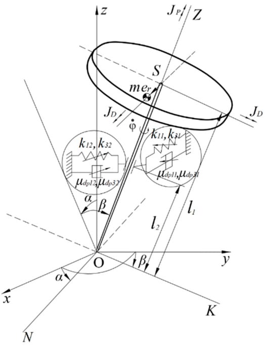
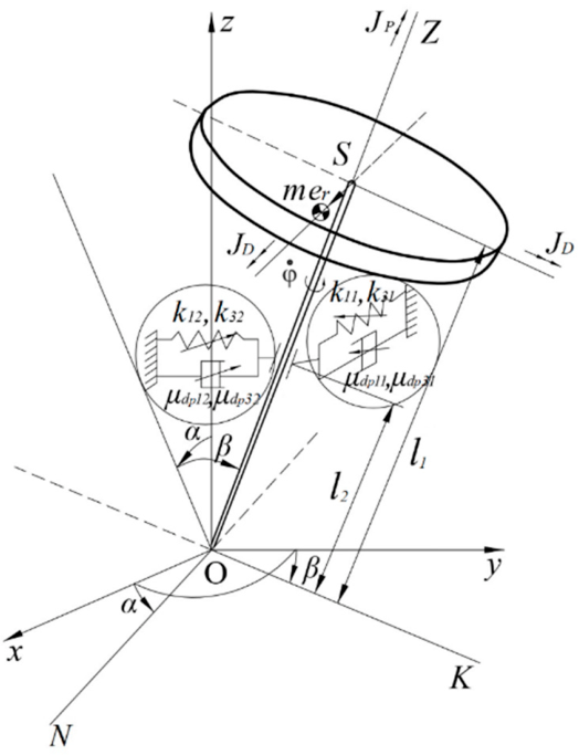
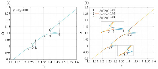
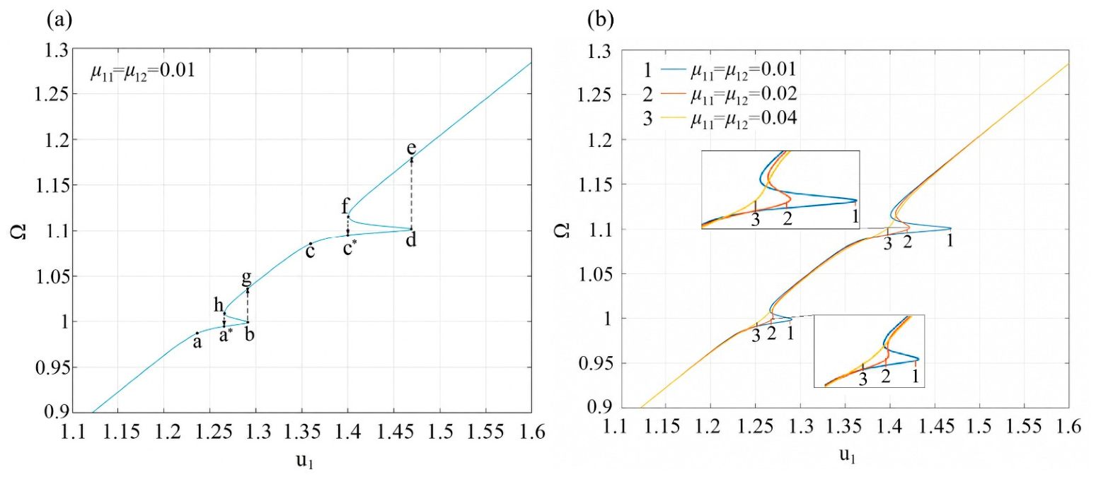
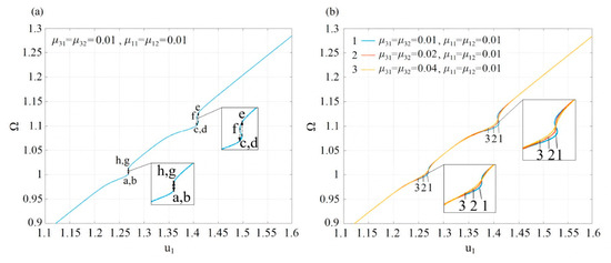
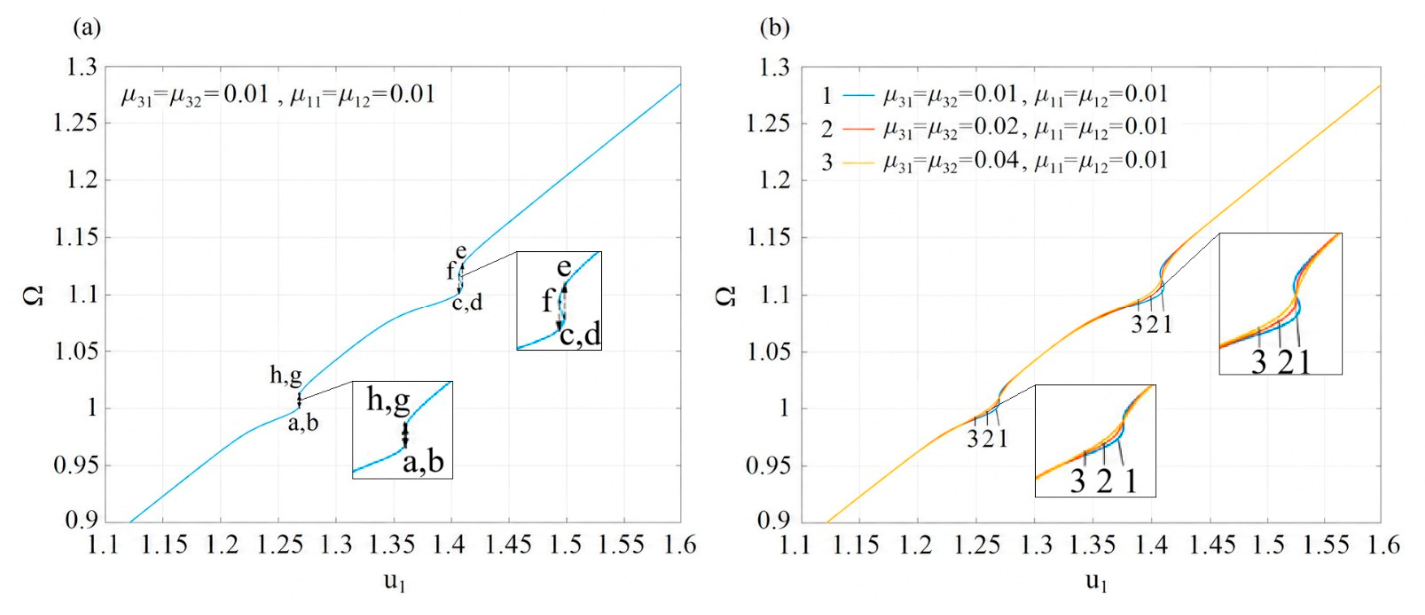
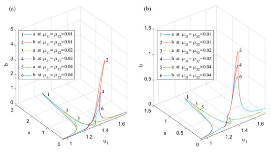
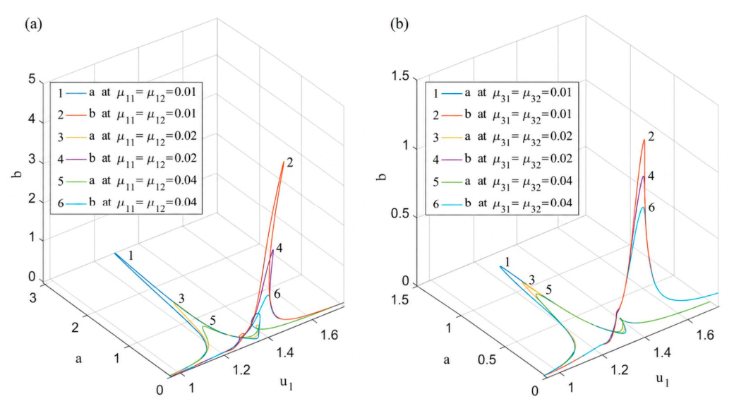
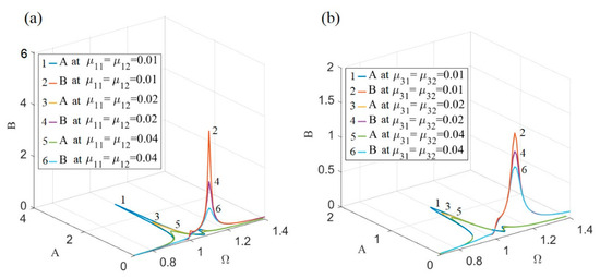
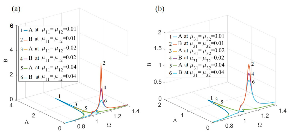
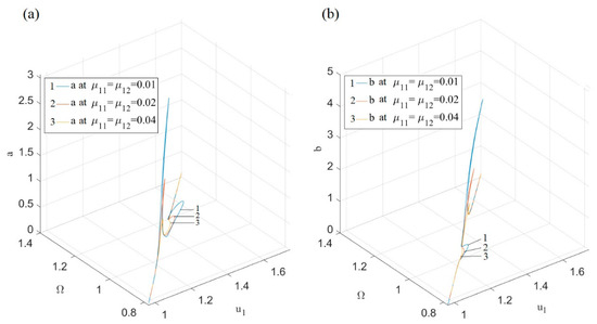
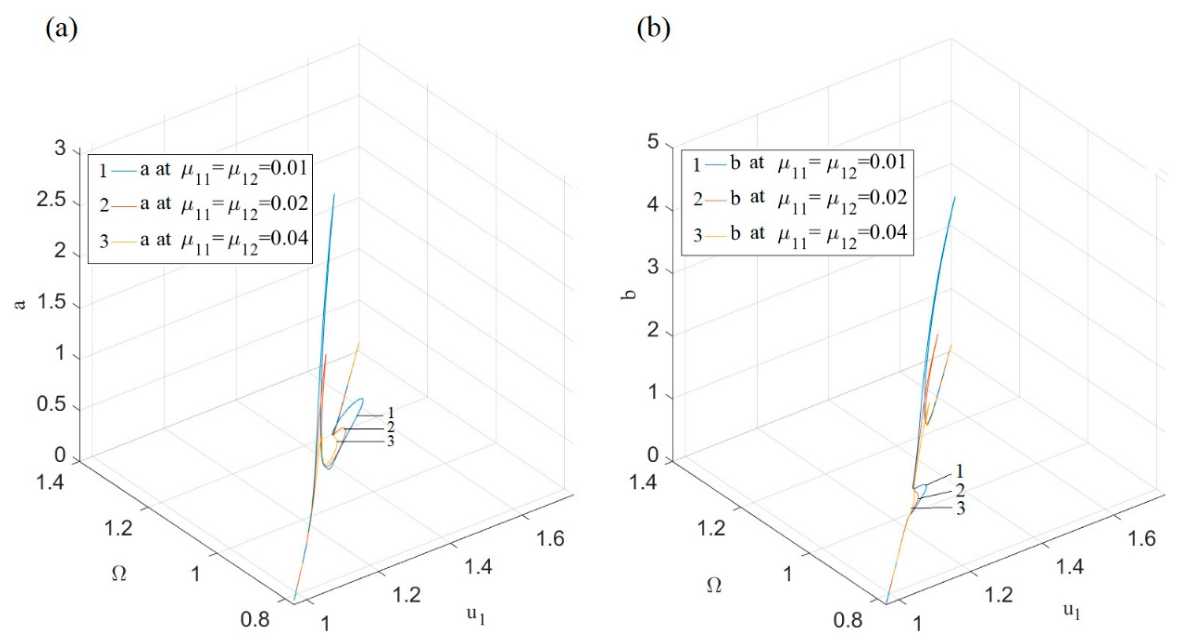
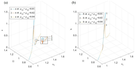
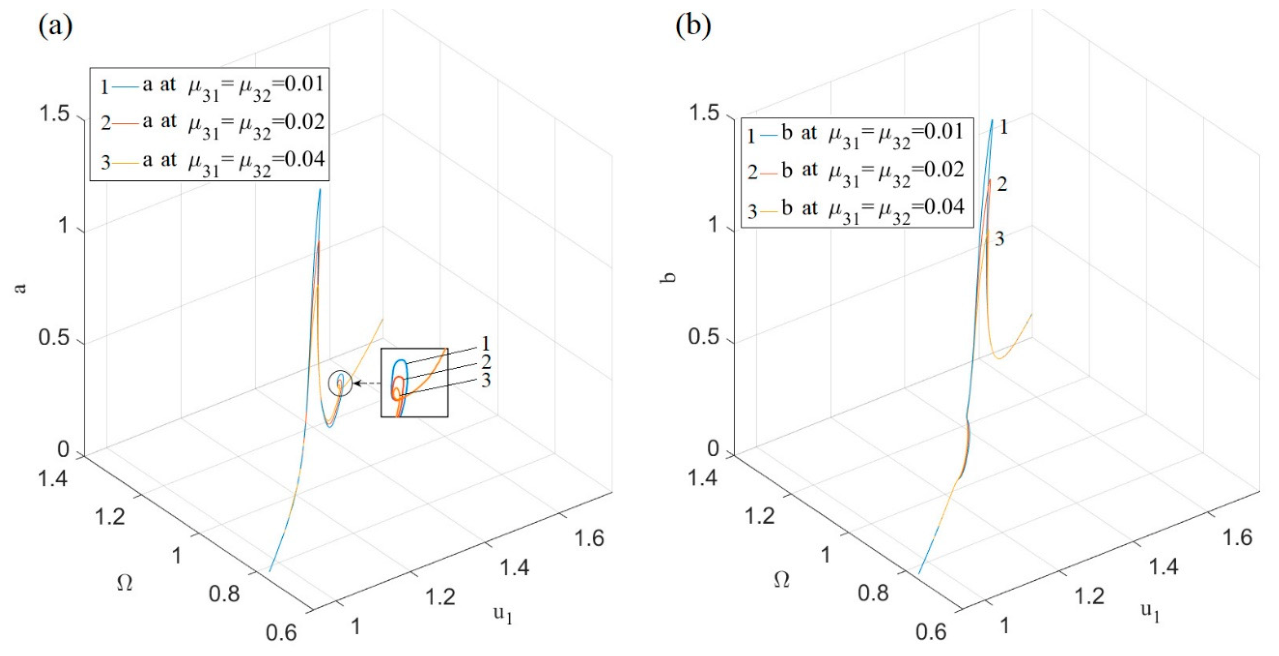
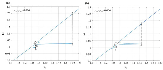
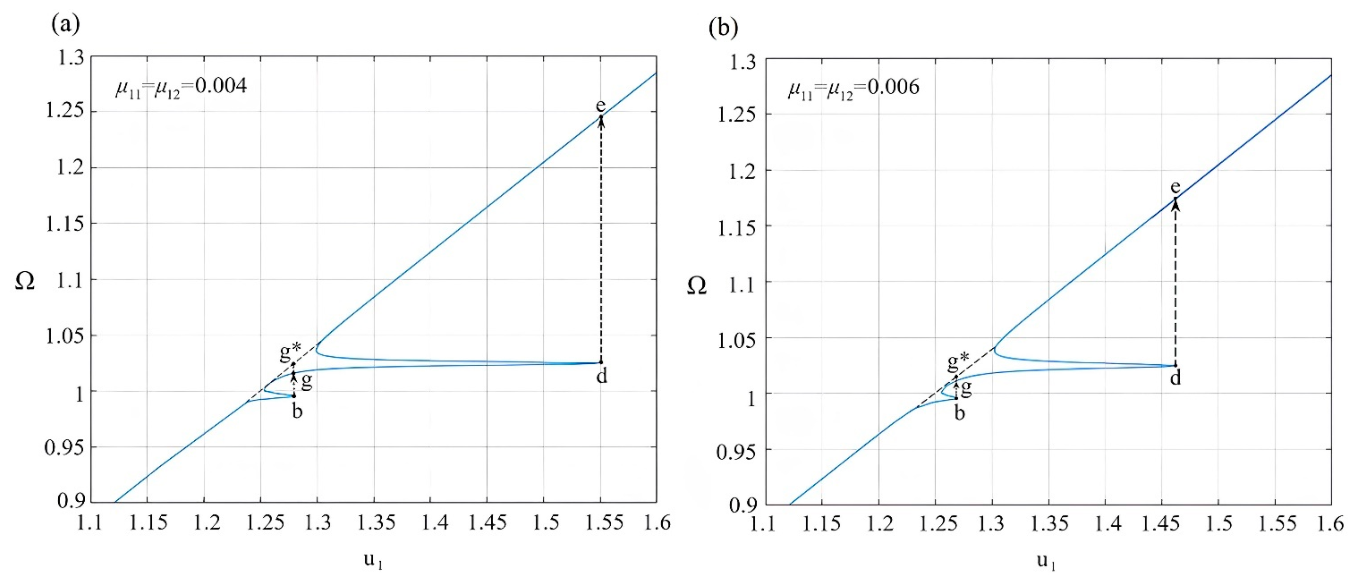
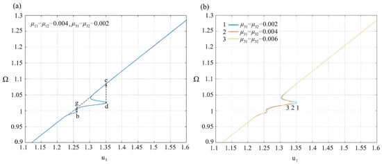
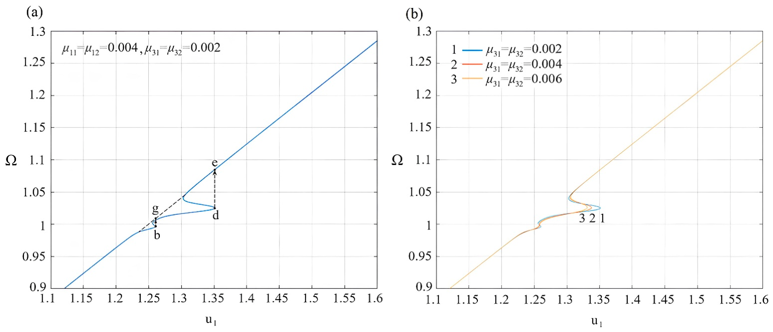
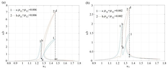
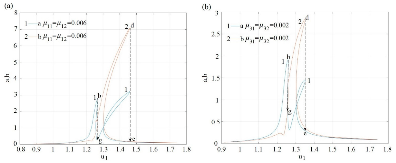
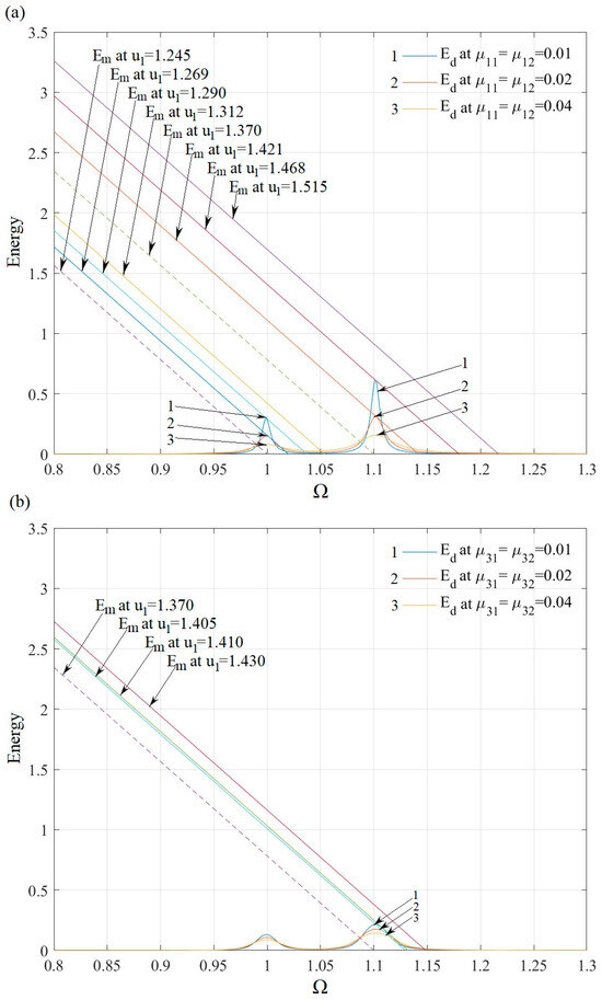
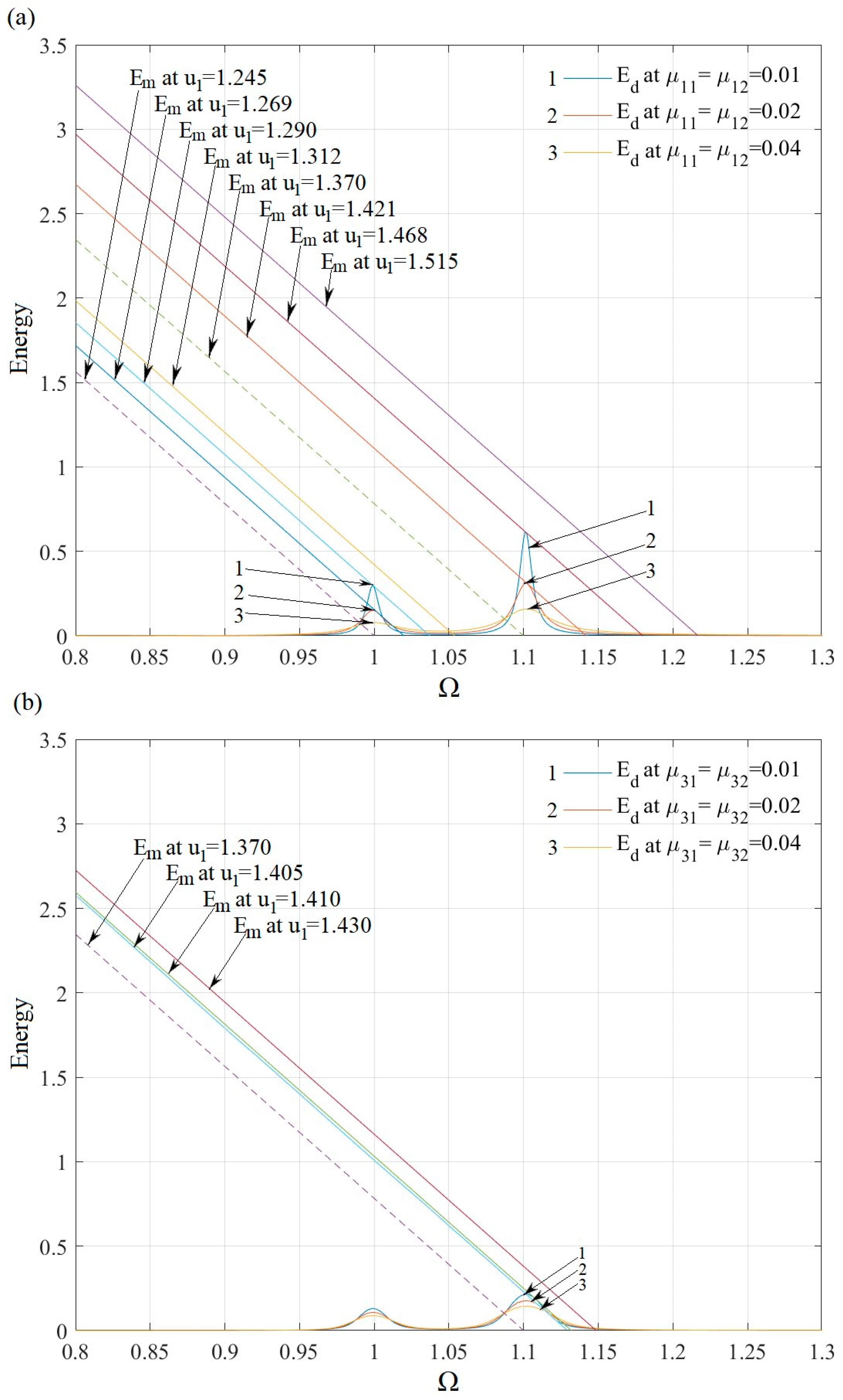
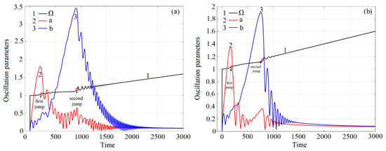
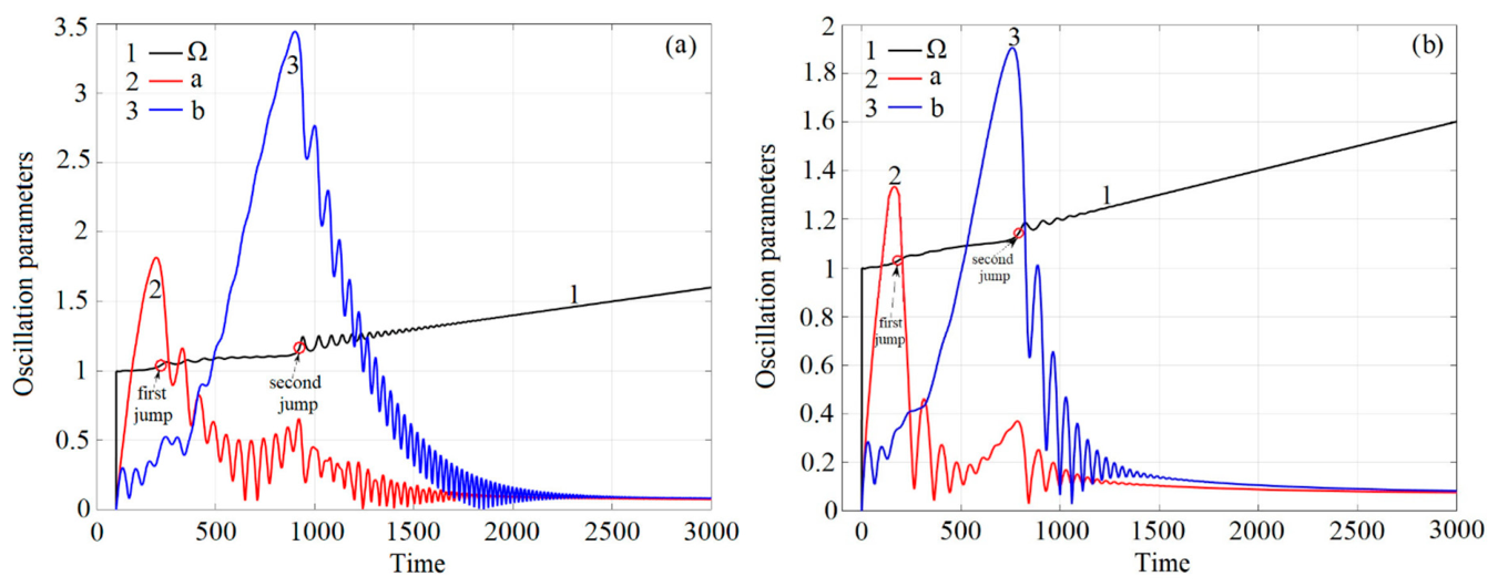
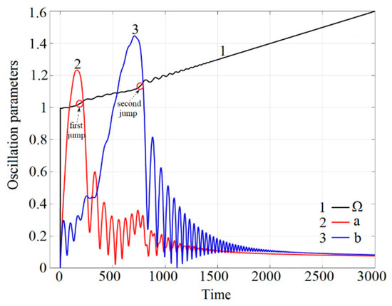
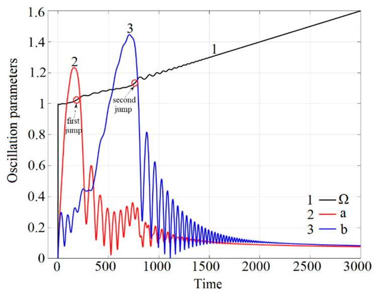
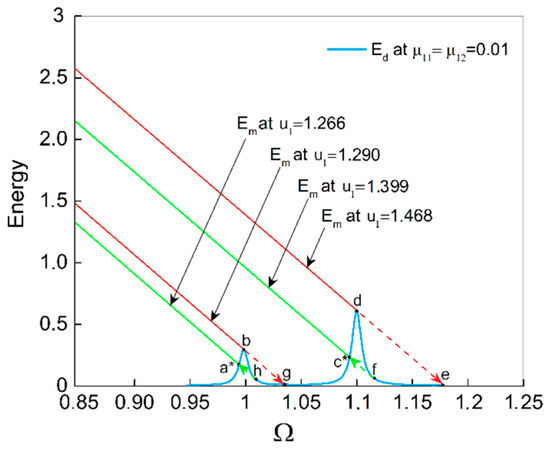
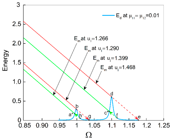
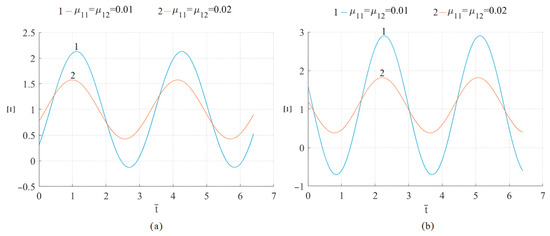
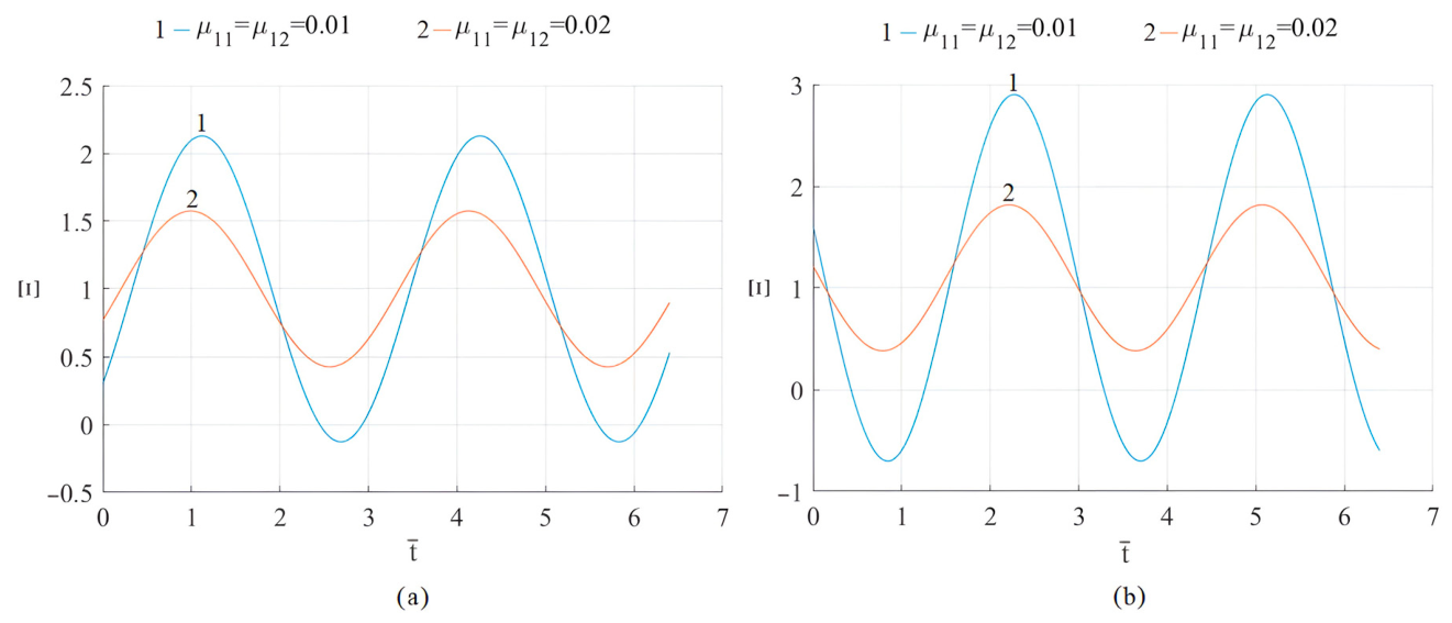
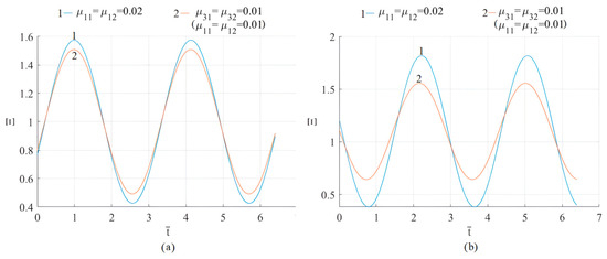
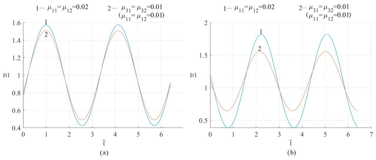
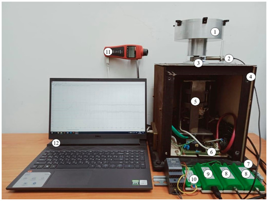
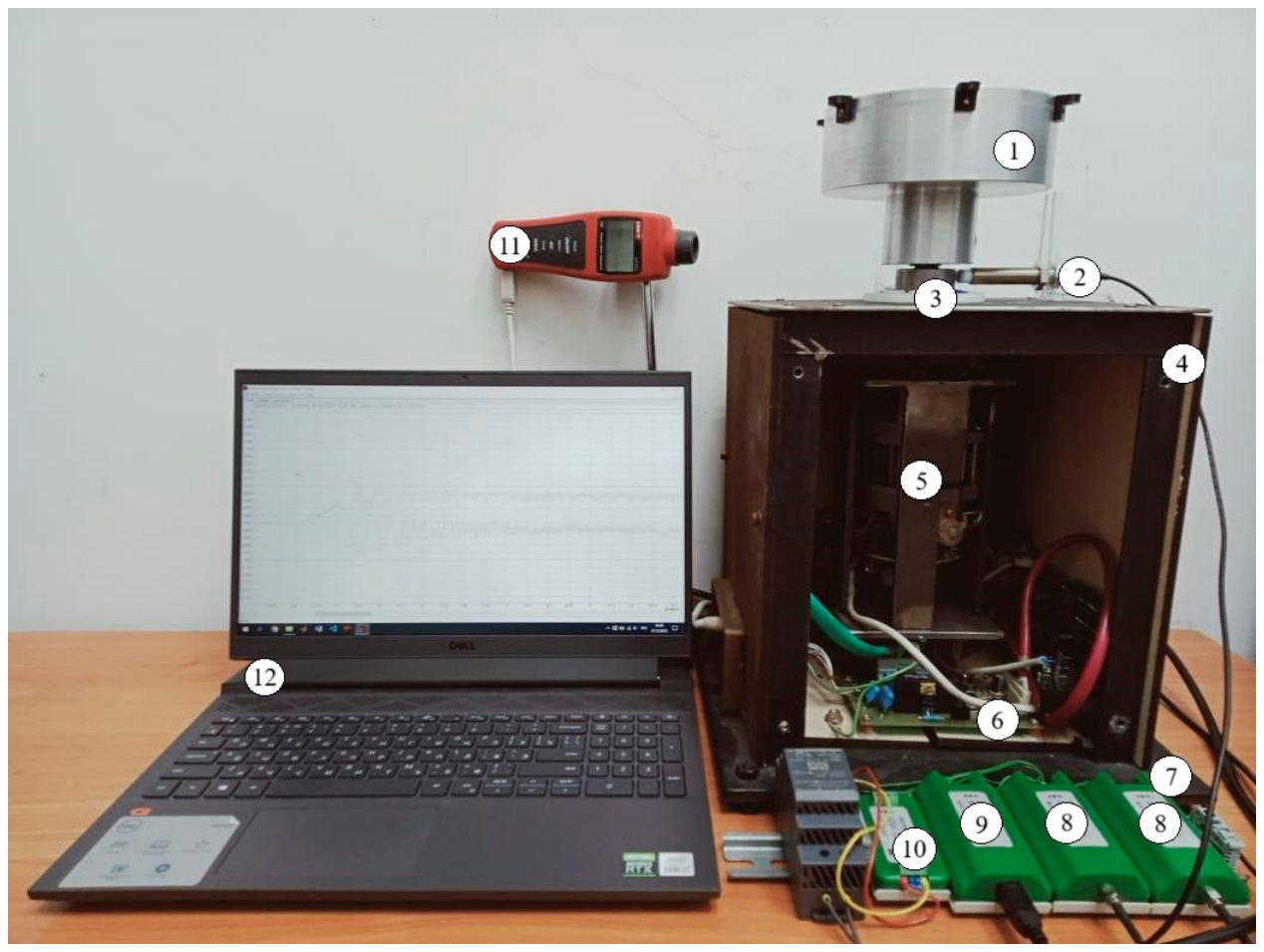
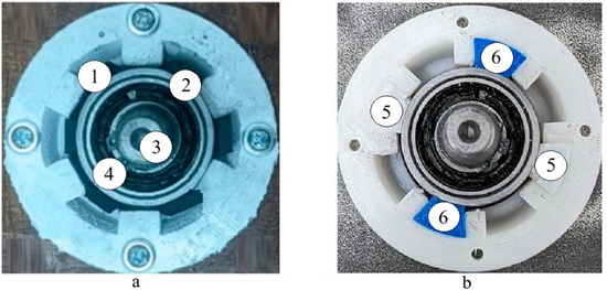
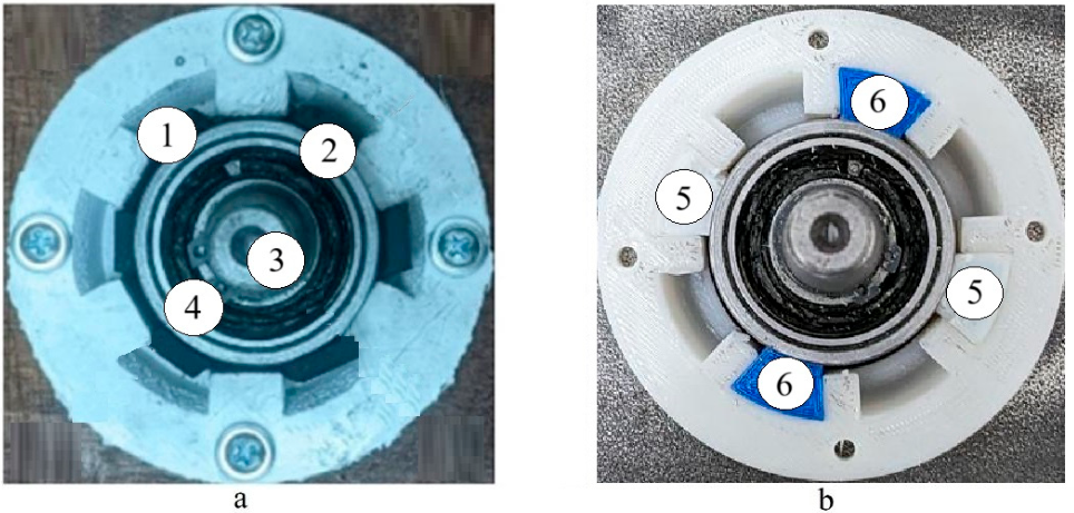
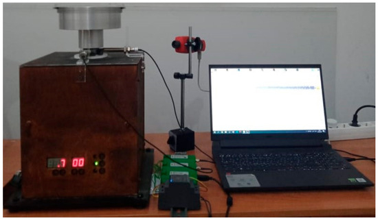
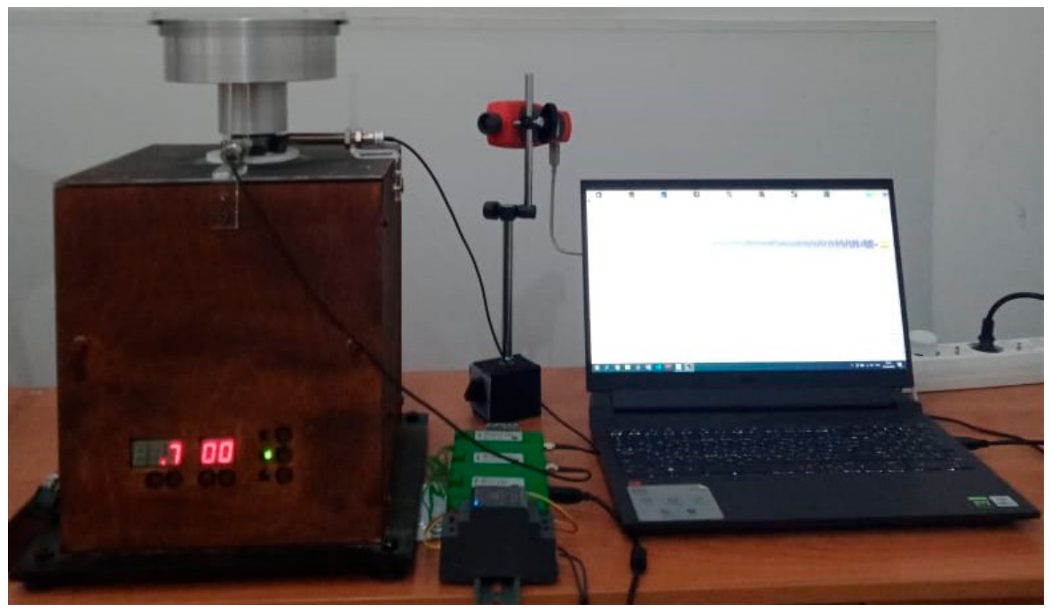
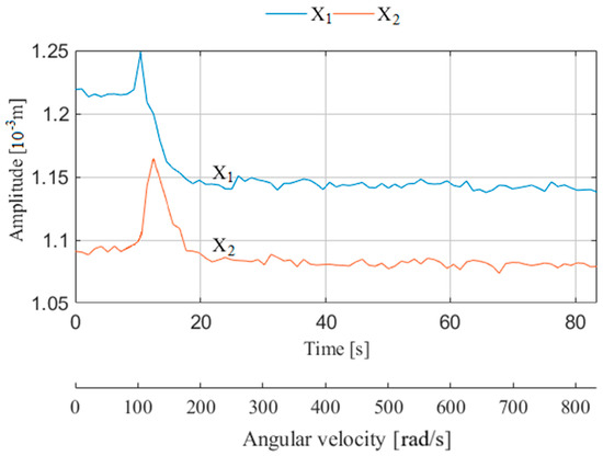
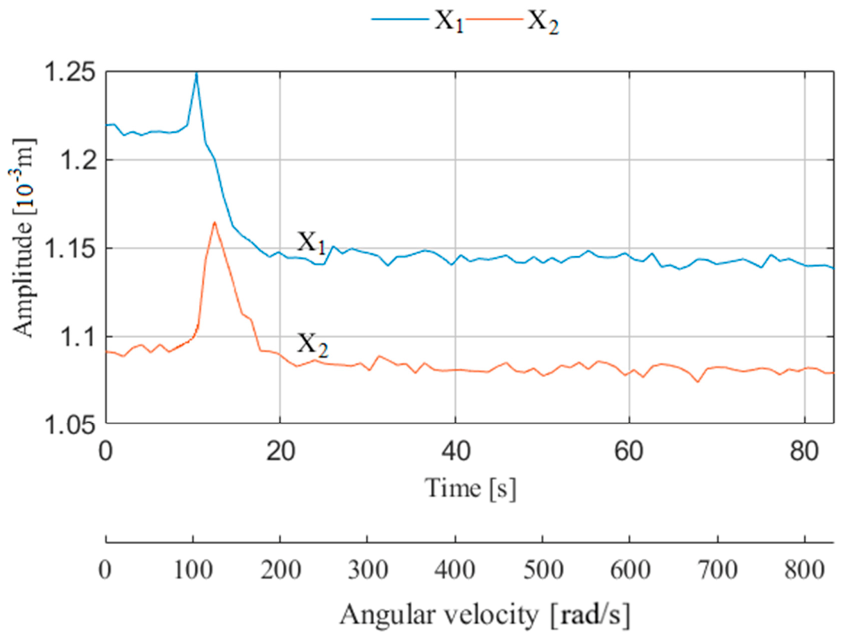
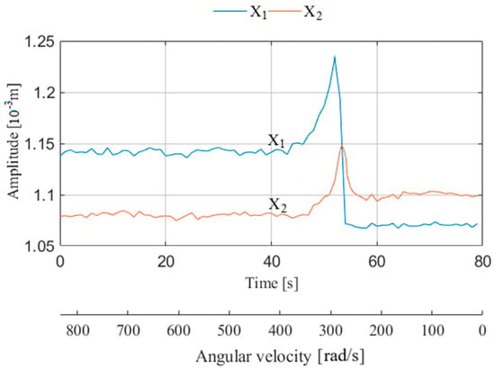
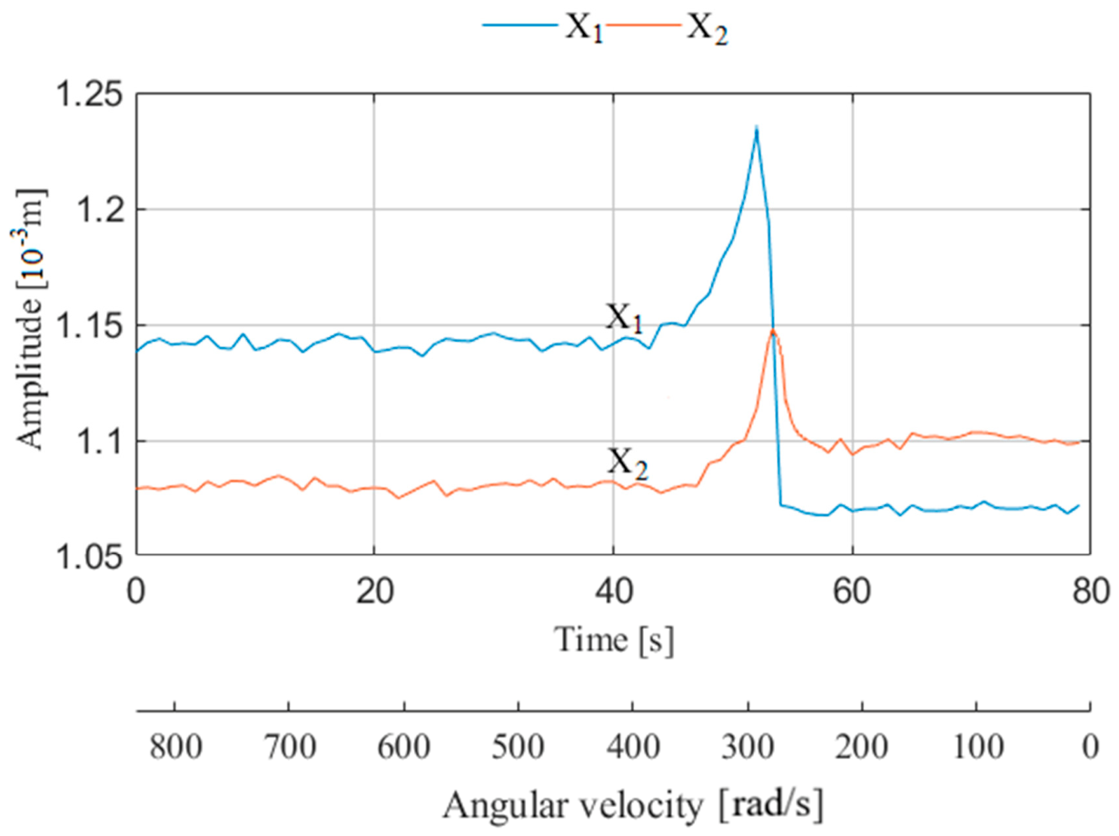
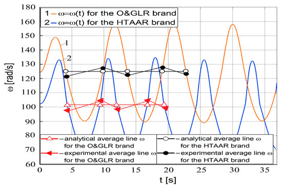
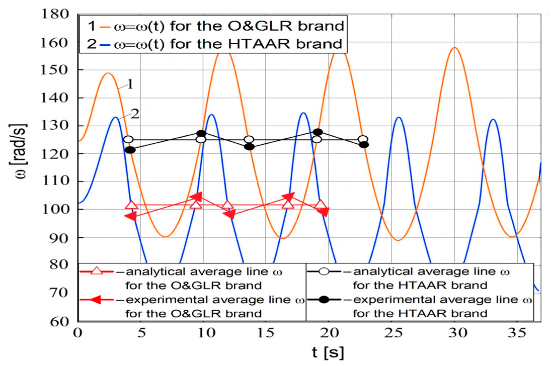
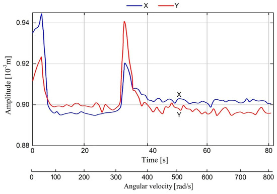
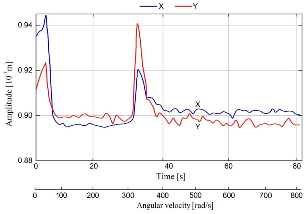
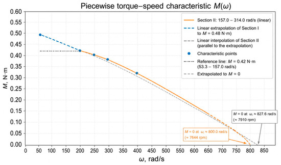
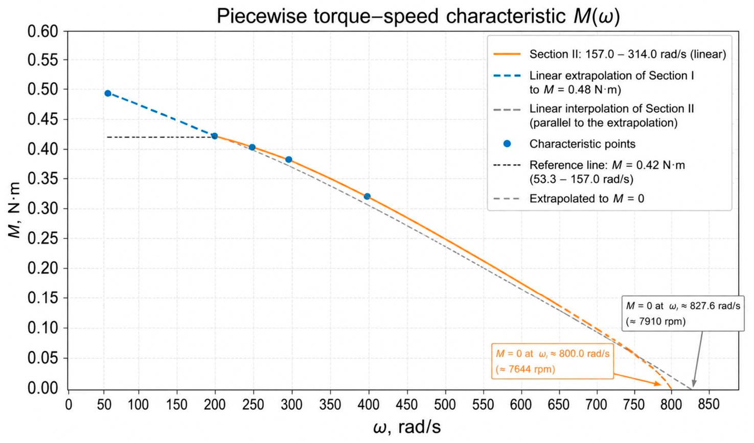
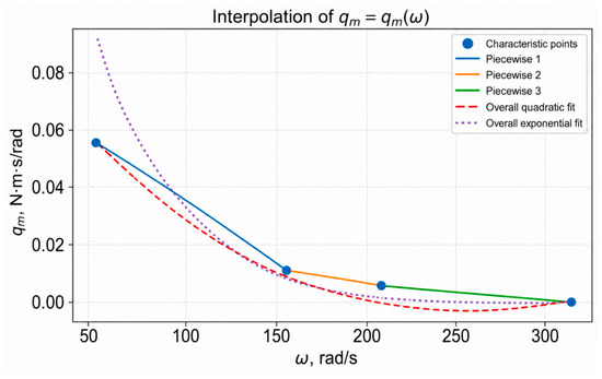
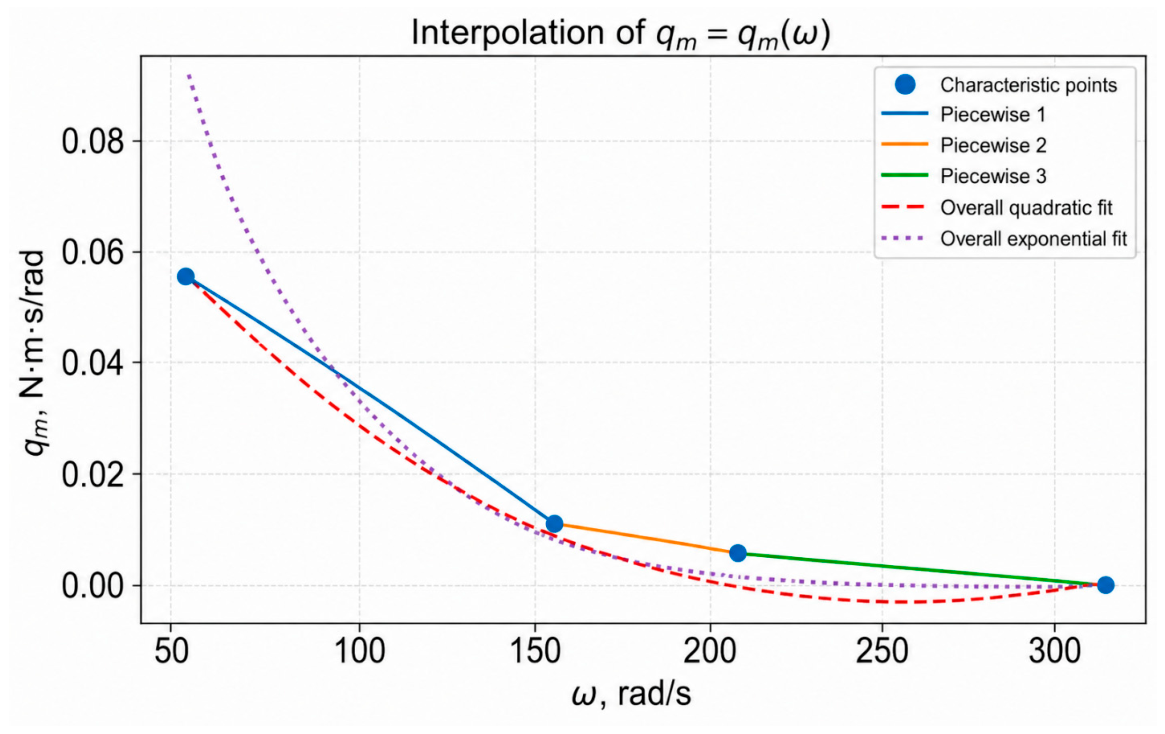
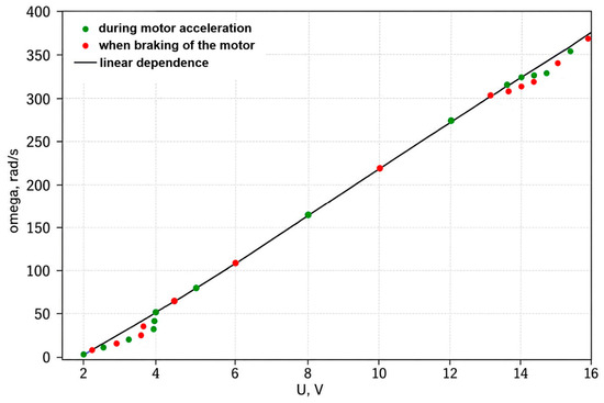
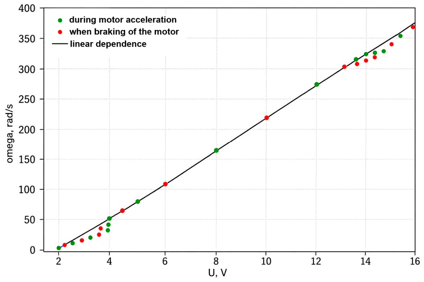
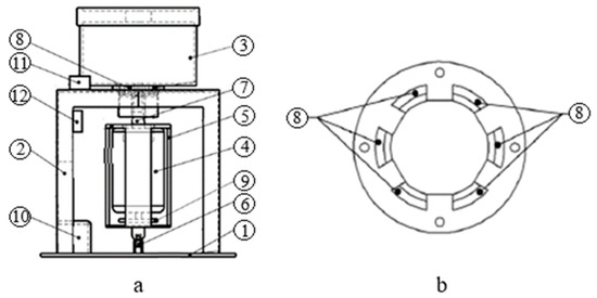
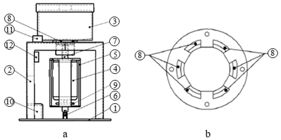

Disclaimer/Publisher’s Note: The statements, opinions and data contained in all publications are solely those of the individual author(s) and contributor(s) and not of MDPI and/or the editor(s). MDPI and/or the editor(s) disclaim responsibility for any injury to people or property resulting from any ideas, methods, instructions or products referred to in the content. |
© 2026 by the authors. Licensee MDPI, Basel, Switzerland. This article is an open access article distributed under the terms and conditions of the Creative Commons Attribution (CC BY) license.