


Abstract
Phishing susceptibility reflects both stable psychological traits and transient user states, but confirmed victim cases remain rare in survey studies. This study evaluated BioHARP, a feasibility framework that pairs an outcome-independent psychometric prior with a prospective bio-adaptive fusion design. Using anonymized respondents (12 strict victims), we constructed 69 pre-incident predictors after excluding administrative metadata, exposure indicators, and post-incident response items. A cost-sensitive TabTransformer was trained without synthetic minority generation and benchmarked against six conventional tabular baselines and FT-Transformer under identical splits, unified preprocessing, and model-appropriate cost-sensitive imbalance handling. Out-of-sample performance was primarily assessed with a 60-seed repeated stratified hold-out protocol with fixed four-positive/thirty-negative test composition. Across the sixty splits, TabTransformer yielded a mean AUC of , whereas CatBoost yielded . On fixed Seed 100, TabTransformer reached AUC and CatBoost AUC ; for the single-init TabTransformer, this was the best-observed split and was therefore interpreted as an optimistic upper-end point estimate. Threshold-dependent metrics were reported separately as an exploratory analysis with explicit leakage labeling. The physiological fusion layer was evaluated as an outcome-informed oracle upper bound, reaching AUC on Seed 100 and , range [0.73, 0.98], across 70 alternative scenario RNG seeds. This result was interpreted strictly as theoretical headroom rather than deployment-calibrated performance. Overall, BioHARP was framed as a feasibility framework with a clearly bounded physiological-fusion design and explicit calibration and sensor requirements for future deployment-ready bio-adaptive detectors.
1. Introduction
Phishing remains a persistent sociotechnical threat because such attacks exploit attention, emotion, and decision-making processes. Although technical controls are indispensable, recent studies increasingly emphasize human-centric, multilayer strategies that account for psychological vulnerabilities [1]. Cognitive evidence further indicates that susceptibility depends on how users allocate attention and apply heuristics under uncertainty, with systematic differences between expert and non-expert behavior [2,3], consistent with heuristic–systematic accounts of victimization [4]. Collectively, these findings suggest that the same user may be cautious in one moment and vulnerable in another, supporting a dynamic view of susceptibility rather than a fixed trait [5,6].
Accordingly, we move beyond static trait-based scoring toward a bio-adaptive evidence layer that captures transient cognitive and affective states. Neurocognitive work indicates that acute stress and specific emotions can temporarily weaken executive control and critical analysis [7,8], creating vulnerability windows that static profiling alone cannot explain. Interdisciplinary decision research likewise suggests that emotional engagement is part of valuation and sense-making, rather than merely noise layered on rational choice [9]. More recent findings show that anger and fear have distinct carryover effects under uncertainty, that self-distancing can attenuate these effects [10], and that mood and confidence shape exploration–exploitation flexibility [11]. At a broader psychophysiological level, stress can speed urgent responding while impairing consequence evaluation when careful deliberation is required [12]. Together, these findings motivate treating fear, anger, anxiety, stress, and broader mood states as operationally relevant inputs to phishing risk.
To ground BioHARP risk estimation in measurable human factors, we first characterize a survey-based psychometric instrument using exploratory and confirmatory factor analysis on anonymized responses, with explicit attention to the limits of same-sample confirmatory evidence. We then construct an outcome-independent predictive feature set of 69 pre-incident predictors (4 demographic variables, 63 Likert-scale psychometric items, and 2 binary pre-incident protective items). Under the strict victim definition, confirmed harm outcomes remain rare (), making conventional empirical risk minimization sensitive to majority-class bias. A cost-sensitive TabTransformer trained with class-weighted binary cross-entropy is therefore used, preserving all original respondent records while increasing the loss contribution of minority-class errors.
In parallel, BioHARP introduces a physiological fusion layer designed to update the static susceptibility prior under transient stress and affective evidence. In the present study, we evaluate this layer through scenario-based physiological evidence rather than through prospectively collected sensor measurements. The fusion analysis is therefore interpreted as a prospective design analysis and, for the outcome-informed oracle upper bound, as theoretical headroom.
Our contributions are as follows:
- We construct an outcome-independent phishing-susceptibility feature set from anonymized survey responses, retaining all respondents while excluding administrative metadata, direct exposure indicators, outcome-defining variables, and post-incident response items from model inputs.
- We report a psychometrically characterized susceptibility profile based on 69 pre-incident predictors, with a three-factor core supported by a pruned same-sample CFA (full six-factor confirmatory validation is not claimed; see Section 3.3), preserving the distinction between pre-incident trait-like factors and outcome-derived labels.
- We implement a cost-sensitive TabTransformer baseline using class-weighted binary cross-entropy to address extreme class imbalance without synthetic minority generation.
- We evaluate the outcome-independent rare-event setting using a fixed Seed 100 hold-out split and a 60-seed robustness sweep, explicitly reporting both recall-oriented performance and split sensitivity.
- We formalize a Bayesian-inspired logit-space risk-amplification rule that adjusts a static susceptibility prior using scenario-based HRV and facial-affect evidence.
- We report an outcome-informed oracle upper-bound fusion analysis to estimate theoretical headroom, while clearly distinguishing it from deployment-calibrated performance.
- We provide differential scenario case studies based on three anonymized profile cases, with User B derived from an anonymized real hold-out survey profile, illustrating how scenario-based physiological evidence can leave low-risk users below a nominal warning threshold, move borderline users above it, and further elevate already high-risk profiles.
2. Related Work
Phishing research is inherently interdisciplinary, spanning social engineering theory, psychometrics, and applied machine learning. A practical challenge is that laboratory-style phishing simulations are susceptible to observation effects (e.g., participants behaving more cautiously when they know they are being tested). Four strands are therefore reviewed in this section, identifying the gap that a bio-adaptive approach addresses.
2.1. Social Engineering Techniques and Structural Vulnerability Modeling
Social engineering attacks do not rely solely on technical exploitation; rather, they operationalize persuasion strategies such as authority, urgency, scarcity, reciprocity, and fear appeals. In structured susceptibility models, persuasive content is often represented as an enticing offer or context, a threat that amplifies perceived consequences, and an enforcement cue that pressures immediate compliance. These formulations translate qualitative manipulation tactics into computable features, but most prior models still treat susceptibility as a fixed trait and do not incorporate temporally varying human states.
In line with human-centric prevention principles, multilayer parametric models have been proposed to operationalize psychological factors as measurable inputs, shifting emphasis from purely reactive technical filtering toward assessing vulnerability drivers that may exist before an attack is encountered [1].
2.2. Psychometric Susceptibility Profiling
A large body of work estimates phishing susceptibility from relatively stable individual differences and demographics (e.g., digital literacy, risk tendency, trust propensity, age, and organizational role). Recent large-scale simulations, such as the two-year longitudinal study by Oner et al. [13], involving more than 8000 employees, empirically show that static demographic and organizational factors strongly correlate with susceptibility and incident-reporting behavior. While this profiling provides a crucial and defensible baseline for organizational risk, it fundamentally captures a static state. It does not explain why the same individual may be cautious in one moment and highly vulnerable in another [14], motivating our approach of augmenting static priors with transient user-state information.
2.3. Machine Learning for Tabular User-Risk Estimation Under Imbalance
Survey-driven susceptibility prediction is a tabular, rare-event learning problem with mixed psychological and behavioral indicators. Transformer-style tabular models can capture interactions among discrete survey responses, but when confirmed victim cases are extremely rare, standard training objectives may favor the majority class. Rather than modifying the empirical survey distribution through synthetic minority generation, the present study adopts a cost-sensitive learning strategy. In preliminary experiments, we evaluated synthetic oversampling (SMOTE) and a diffusion-based tabular generator (TabDDPM); on this rare-event dataset, both approaches either degraded honest held-out performance or, when synthetic physiological evidence was generated conditionally on the outcome label, introduced leakage that inflated apparent results without reflecting genuine signal. Cost-sensitive learning is therefore adopted, which preserves all original respondent records and the empirical survey distribution while adjusting the penalty assigned to minority-class errors through a class-weighted loss function.
Building on our prior work evaluating the performance impact of social engineering vectors and proposing multidimensional measurement constructs [15], we treat the survey-driven classifier as a baseline susceptibility estimate that is necessary but not sufficient for operational defense, especially when susceptibility is better explained through dynamic cognitive processing models [2,3,4,5,6]. Although our setting is tabular and human-centric rather than signal-processing, the additive log-odds structure of our fusion rule (Section 3.5) belongs to a broader tradition of additive multimodal feature fusion. In that tradition, independent evidence streams are combined into a single decision score. Analogous multimodal-fusion designs appear in adjacent detection and signal-processing domains, including Fourier-information fusion for image restoration [16] and cross-attention-based spatial–frequency–optical–flow fusion for AI-generated video detection [17]. We adopt the same additive-evidence design in the human-factors setting that is the focus of the present paper.
2.4. Physiological and Affective Computing Signals for Security
In parallel, affective computing and psychophysiology studies show that stress and emotion are reflected in signals such as HRV and facial affect. However, these signals are often evaluated with laboratory-grade sensors or in settings disconnected from cybersecurity decision points. Bridging this gap requires a mechanism that can update risk estimates online while remaining interpretable to practitioners.
This perspective is consistent with evidence that affective states bias judgment and risk processing (e.g., fear and anger in risk appraisal) [7,8]. More recent decision-making research suggests that these effects are emotion-specific rather than a generic arousal effect: under uncertainty, incidental anger can slow avoidance of disadvantageous risky options relative to fear when decision-makers remain self-immersed in the eliciting event [10]. Mood and confidence also appear to influence how flexibly individuals switch between exploration and exploitation, thereby shaping learning and performance in uncertain environments [11]. Review evidence on stress and glucocorticoids further suggests a dual pattern in which stress can facilitate speeded responses in urgent conditions but degrade consequence evaluation and increase risky choice in more complex settings [12]. Neural evidence additionally indicates that discrete emotions such as happiness, fear, and sadness can differentially modulate decision-related cross-frequency brain networks, reinforcing the idea that affective state is a structured input to choice rather than a single undifferentiated arousal signal [18]. This line of evidence aligns with emerging cybersecurity work that treats physiological signals as correlates of susceptibility and stress responses at decision time [19], and with broader theories that conceptualize prolonged “unsafe” states as shaping perception and health-relevant behavior [20].
Recent conceptual frameworks, such as the mitigation model proposed by Abroshan et al. [21], emphasize that behavior and emotion (e.g., during crisis periods) strongly influence phishing success, thereby supporting dynamic risk scoring. Building on this perspective, our framework operationalizes affective vulnerability through a computable Bayesian-inspired fusion rule designed to support future physiological channels such as HRV and facial affect.
Taken together, these strands motivate our design: (1) a psychometrically characterized static prior, (2) a cost-sensitive tabular estimator for prior risk evaluated under a transparent repeated hold-out protocol that exposes split sensitivity rather than masking it, and (3) an explainable bio-adaptive logit-space risk-amplification rule designed for physiological evidence integration.
3. Materials and Methods
3.1. Dataset and Outcome-Independent Feature Construction
The raw survey dataset contains anonymized respondent records. We performed data cleaning column-wise rather than row-wise; no respondents were removed. To construct an outcome-independent predictive feature set, we excluded administrative metadata, direct exposure indicators, outcome-defining variables, and post-incident response or mitigation items before model training. The final predictive input consisted of 69 pre-incident predictors (4 demographic variables, 63 Likert-scale psychometric items, and 2 binary pre-incident protective items), all encoded on their original ordinal or binary response scales. The strict victim label was derived separately from a confirmed harm outcome and was not included among the predictive features. The end-to-end framework is summarized in Figure 1.
Figure 1.
BioHARP workflow: Outcome-independent feature construction from survey responses, psychometric validation, cost-sensitive TabTransformer prior estimation, and scenario-based physiological fusion for adjusted risk scores.
3.2. Strict Victim Label Definition
Strict victims were defined as respondents reporting a confirmed harm outcome after a phishing incident. This definition yielded 12 positive cases and 124 non-victim cases. Because the outcome-defining item was used only for label construction and removed from model inputs, the classifier was trained solely on pre-incident or trait-like psychometric susceptibility indicators.
3.3. Psychometric Instrument and Validation
To ground the static prior in measurable human factors, we collected survey responses from participants with diverse digital proficiency. The psychometric layer was used to characterize the internal structure of the susceptibility instrument and to support interpretation, with explicit attention to the limits of same-sample confirmatory evidence (Section 3.3). Construct-level scores were used for psychometric validation and descriptive analysis; the downstream TabTransformer classifier used item-level encoded survey responses rather than the construct-level aggregate scores.
3.3.1. Participants and Demographics
Participants were recruited from a real-world university/workforce context rather than a single homogeneous student cohort. The sample covered ages 18–50 (mean 28.4, SD 4.2) and included mixed educational backgrounds (60% undergraduate, 25% graduate, 15% high school).
3.3.2. Measurement Instrument
The inventory operationalizes multiple latent constructs commonly implicated in phishing susceptibility. Items were presented as short statements and rated on a Likert-type response scale. The instrument includes items spanning constructs commonly associated with phishing susceptibility (e.g., digital literacy, risk perception, and trust/suspicion), along with related behavioral dispositions.
Although these domains provide an intuitive design-time grouping, the exploratory factor analysis reported below suggests a six-factor latent grouping of the item pool; this grouping is treated as descriptive rather than confirmatory at the present sample size, for the reasons set out in the validation subsection. Items were coded so that higher scores consistently indicate higher susceptibility-relevant levels for the corresponding construct (with reverse-coding where applicable). For psychometric analyses, construct scores were computed by averaging item responses within each scale; for predictive modeling, the classifier consumed the encoded item-level responses directly.
3.3.3. Factor-Analytic Validation
We evaluated factorability and construct validity using standard EFA/CFA diagnostics. The overall Kaiser–Meyer–Olkin (KMO) measure of sampling adequacy is on the 63-item Likert pool (and on the full 69-feature set), and Bartlett’s test of sphericity is significant (, ). The overall KMO falls in the Kaiser’s “mediocre to middling” band; we report this honestly rather than only describing it as “acceptable.”
Per-item KMO values reveal additional fragility that an overall summary alone would hide. Among the 63 Likert items, 1 item falls in the meritorious band (), 19 in the middling band (–), 25 in the mediocre band (–), 11 in the miserable band (–), and 7 items fall below the conventional 0.50 cut-off. The seven sub-threshold items concentrate at the periphery of the six-factor solution rather than at its three-factor core. The full sorted per-item KMO vector for all 63 Likert items is reproduced in Appendix A; we treat these item-level diagnostics, together with the full-pool CFA fit reported below, as the primary evidence on which the six-factor structure should be evaluated.
For CFA, we report fit indices across pruned high-loading subsets and across the full item pool in Table 1. The pruned 3-factor/9-item configuration (top-3 items per factor) shows adequate fit by conventional thresholds (, ), the 4-factor/12-item configuration shows acceptable fit, and the 5-factor/15-item configuration shows marginal fit. A 6-factor pruned configuration is not estimable because the sixth factor recovers fewer than three items with sufficiently high loadings. The full 63-item/6-factor CFA fit on the same sample (N = 136) is materially weaker (CFI , RMSEA ), indicating that the instrument has a robust 3-factor core and an additional latent structure that does not survive a strict full-pool 6-factor CFA at the present sample size. Internal-consistency estimates (Cronbach’s ) were computed at the scale level during instrument development but are not used as evidence for confirmatory factor validity in the present manuscript, and are not reported here because the present paper concerns predictive feasibility rather than scale construction.
Table 1.
Confirmatory factor analysis fit indices across pruned high-loading subsets and the full item pool (N = 136). Pruned variants take the top-3 items per factor by absolute EFA loading. The full-pool 6-factor fit is included for transparency; the value corresponds to the pruned 3-factor/9-item configuration.
Three honest conclusions follow. First, the instrument is best characterized as having a three-factor core supported by a pruned same-sample CFA (CFI , RMSEA ), rather than as a confirmed measurement model on an independent sample. We make this distinction because a same-sample EFA followed by a top-loading-pruned CFA is by construction descriptive of the present 136 respondents, not a cross-validated confirmatory test. Second, the six-factor solution should be treated as descriptive and exploratory rather than confirmatory, especially in view of relative to a 63-item pool (ratio approximately respondents per item, well below the rule-of-thumb minimum of 5–10 for stable confirmatory factor recovery) and in view of the per-item KMO distribution above. Third, the predictive layer described in Section 3.4 does not depend on the latent structure being recovered exactly at six factors, because it consumes item-level encoded responses rather than construct-level aggregate scores. The relationship between the characterized psychometric structure and the predictive model is detailed in Section 3.3.4 and Section 4.5, and the construct-versus-item ablation reported there quantifies the predictive cost of moving from item-level inputs to construct-level aggregates. We make no claim of confirmatory six-factor validity on the present sample.
3.3.4. From Psychometric Structure to Predictive Features
The factor-analytic results above serve two complementary purposes that should be distinguished. First, the exploratory and confirmatory analyses are used to characterize the latent structure of the survey instrument and to support its interpretability, and the items with the highest standardized loadings on each factor are identified. Second, the predictive classifier in Section 3.4 consumes the item-level encoded responses rather than construct-level aggregate scores. We adopt item-level inputs for three reasons that are specifically relevant to the present rare-event regime. First, with only twelve strict victim cases, aggregating items into a construct means discarding within-construct variance that the classifier could otherwise exploit. Second, transformer-style embeddings learn item-specific contextualization; thus, collapsing items to a mean defeats the architectural feature that motivated the model choice. Third, construct-level scores can still be reported alongside the predictive output as a post hoc interpretability layer rather than as a model input. An explicit construct-level versus item-level ablation that quantifies this design choice across six baseline classifiers is presented in Section 4.5.
3.4. Cost-Sensitive TabTransformer Baseline
The static susceptibility prior is estimated using a TabTransformer classifier [22], an attention-based architecture for tabular data. Prior work has shown that TabTransformer remains competitive with classical baselines under careful regularization, although gradient-boosting methods often dominate on small datasets [23]. The model receives the 69 encoded predictors as categorical inputs (4 demographic items, 63 Likert-scale psychometric items, and 2 binary pre-incident protective items). Learned embeddings of dimension 32 are used to represent item responses, and the contextualized representations are passed through a Transformer encoder with 4 layers and 4 attention heads before binary classification. Because all predictors are discrete survey responses, estimation relies on contextualized categorical embeddings rather than a mixed numeric/categorical pipeline.
To address extreme class imbalance without fabricating additional behavioral profiles, we use a cost-sensitive training objective. The final multilayer perceptron produces a single logit and is optimized using class-weighted binary cross-entropy in logit form:
where z is the predicted logit, is the strict victim label, and is the positive-class weight computed from the class distribution of the training split. This weighting increases the penalty for misclassified victim cases while preserving the original respondent records and empirical survey distribution. In implementation, this corresponds to BCEWithLogitsLoss (pos_weight = pos_weight), where pos_weight is computed dynamically from the training labels as . The training configuration is summarized in Table 2. Optimization uses AdamW with decoupled weight decay, a fixed number of epochs (full-batch over the training fold), and fixed random seeds. We do not apply synthetic minority generation. Threshold-dependent metrics are reported in two clearly separated blocks (Section 4.2): the operating point, which was selected on the fixed Seed 100 hold-out split, is therefore retained only as exploratory test-tuned analysis and explicitly labeled as such throughout; leak-free operating points are selected by F1-maximization on the out-of-fold predictions of a 5-fold stratified cross-validation of the training fold only, with the model then retrained on the full training fold and evaluated once on the held-out test set. Both blocks are labeled, with the leakage status of each metric summarized by evaluation type in Section 4.2.
Table 2.
TabTransformer training configuration used throughout this study. The Seed 100 hold-out and 60-seed sweep both follow this configuration; threshold selection is described in Section 4.2.
Notation Dictionary
- z: Predicted logit produced by the cost-sensitive TabTransformer.
- y: Strict victim label used for supervised learning.
- : Positive-class loss weight.
- : Static susceptibility probability from TabTransformer.
- : Event-wise updated posterior risk score.
- : Dynamic risk multiplier at decision event t.
- : Stress and emotion components of .
- : Decision threshold used to map probabilities to class labels.
3.5. Bio-Adaptive Physiological Fusion Engine
The fusion layer is designed as a prospective physiological update mechanism, but the present study evaluates it using scenario-based physiological evidence rather than prospectively collected sensor measurements. The static classifier output is treated as , and the fusion layer produces an adjusted risk score in logit space:
We refer to as an adjusted risk score rather than as a calibrated Bayesian posterior, because the multiplier is a structured composite of literature-motivated heuristic evidence terms rather than an empirically estimated likelihood ratio. The fusion layer is a Bayesian-inspired logit-space risk-amplification rule rather than a fully calibrated probabilistic sensor model. Because the constituent terms and are non-negative by construction, the rule is one-sided: values of raise the static susceptibility prior under stress and affect evidence, while the present formulation is not intended to model protective physiological states. A bidirectional update with signed evidence terms would require prospective sensor calibration and is discussed in the Limitations. This logit form is numerically stable and interpretable. Risk changes can be traced directly to explicit stress and affect terms, which is consistent with emerging affective-computing directions in cybersecurity that treat physiological signals as measurable correlates of susceptibility shifts [19].
3.5.1. Risk Multiplier Design and Stability
To avoid notation ambiguity, we use t in this fusion subsection as a discrete phishing-decision event index (). The risk multiplier aggregates two evidence streams: physiological stress () and emotional affect ().
To guarantee bounded behavior and transparent attribution, we define the domains as follows: , , , , with fixed literature-motivated heuristic coefficients .
The physiological stress term uses a bounded relative drop function :
Thus, the components are tightly bounded: , , and . The final logit-space update, given earlier as the defining fusion rule, ensures . Because the logit transform is undefined at , all prior probabilities are clipped to the open interval with before applying the fusion rule. This convention is applied uniformly to every baseline backbone in the all-prior oracle analysis of Section 4.7, including the tree-based models that can otherwise return exact 0 or 1 probabilities on a finite ensemble. A deployable implementation would additionally require an explicit probability-calibration step on the prior before fusion, because class-weighted training distorts the raw probability scale; the clipping convention above keeps the rule numerically well defined but does not by itself produce calibrated posteriors.
This model is an event-wise update rule rather than a recursive filter. Classical asymptotic convergence limits therefore do not apply, because risk is recomputed independently at each event using current evidence. As a result, accumulation effects are avoided and outputs remain bounded in by construction. The parameter domains, defaults, and functional rationales for , , , , and the operating threshold are summarized in Table 3.
Table 3.
Parameter domains, defaults, and functional rationale.
The default coefficients (, , ) are literature-motivated heuristic defaults rather than parameters fit to the present dataset or derived as numerical constants from any single citation. They were chosen to respect two qualitative constraints that the affective-state and stress–decision-making literature establishes, while leaving the specific numerical magnitudes open for prospective recalibration. The first qualitative constraint is the ordering : fear is documented to engage prefrontal-cortex stress signaling and impair executive control more strongly than incidental anger in acute-threat appraisal [7], and behavioral decision-making work shows that fear shifts risk appraisal more strongly than anger under uncertainty [8,10]. The second qualitative constraint is a bounded operating range for that keeps the multiplicative correction in the same order of magnitude as the static prior. Under the chosen triple, and the additive logit term is bounded as , which is the same order of magnitude as a typical static-prior logit and therefore avoids overwhelming the prior with a single fusion update. Effect-size summaries in the stress and glucocorticoid decision-making literature [7,12] are consistent with this bounded range. We do not claim that the specific numerical triple is derived quantitatively from these citations; the citations motivate the ordering and the bounded range, while the magnitudes are chosen heuristically, subject to those constraints and remain open for prospective recalibration. A sensitivity analysis across alternative coefficient values is reported in Section 4.9 (representative posterior shifts under varying in the opening paragraph, and an oracle-AUC sweep across joint and one-at-a-time low/default/high perturbations of , , ), where the qualitative behavior of the rule is shown to be robust to perturbations of each coefficient. Across datasets, sensor stacks, or model families, the weights should be recalibrated against the deploying population’s matched physiological data; in the absence of such matched data, for the reasons set out in Section 5.7, the present values are reported as literature-motivated starting defaults rather than as a final calibration.
3.5.2. Missing-Sensor Handling (Modular Fusion)
In operational settings, one or more sensor streams may be unavailable (e.g., camera disabled, watch not worn). Because the fusion engine is modular, unavailable evidence terms are set to zero:
- Full sensing: .
- HRV-only: .
- Face-only: .
- No sensors: (static prior only).
3.6. Scenario-Based Physiological Evidence
In the present evaluation, HRV and facial-affect values are treated as scenario-level physiological evidence rather than as prospectively recorded biometric measurements. The HRV terms and are millisecond-valued scalar HRV proxy inputs used to demonstrate the fusion rule; they are not derived from a live wearable preprocessing pipeline. Similarly, and are scenario-level affect probabilities rather than calibrated outputs of a deployed camera model. A prospective implementation would need to specify the HRV summary statistic, aggregation window, artifact filtering, face-analysis model, temporal smoothing, and calibration procedure.
3.6.1. HRV Scenario Channel
Heart rate variability (HRV) is used as a proxy for acute stress [24,25]. For scenario evaluation, we define a baseline (default scenario scalar 50 ms) and compute a non-linear stress activation score from the scenario value . Although population-level HRV ranges are well established, resting HRV varies substantially across individuals; a deployable system would therefore set per user from an initial calibration window rather than from a single population default, so that the stress term reflects each user’s own deviation from baseline. The exponent in introduces mild nonlinearity: small day-to-day fluctuations are down-weighted, whereas acute HRV suppression events are emphasized.
3.6.2. Facial-Affect Scenario Channel
Fear and anger probabilities are treated as scenario-level affect inputs throughout the present evaluation. In a prospective implementation, these terms would be supplied by an established facial-affect recognition model. One example is the DeepFace framework [26], which exposes a categorical facial-expression analysis module that includes fear and anger among its output categories. In a prospective implementation, the specific model version, training corpus, benchmark performance, and per-deployment calibration procedure would need to be documented before the returned probabilities are consumed as and , together with appropriate temporal smoothing. The role of the fusion layer is not to re-derive affect recognition, which is an established capability, but to formalize how a detected affective state, such as fear or anger, mathematically raises the susceptibility score through the penalty term . In the present manuscript, these probabilities are used as scenario inputs to evaluate the behavior of that penalty mechanism.
3.7. Evaluation Protocol
The primary measure of out-of-sample performance is a 60-seed repeated stratified hold-out evaluation. The protocol is a Monte Carlo cross-validation style repeated hold-out: each seed in the range produces an independently sampled random split with exactly four positive and thirty negative test cases, and the model is retrained from scratch on the remaining 102 records. This generates 60 stratified hold-out estimates of out-of-sample performance per model. Because the test sets share the same underlying 136-respondent pool, the 60 estimates are not statistically independent in the sense of new-respondent replications; they characterize variance across random splits of a fixed sample.
This design was selected in preference to a single stratified k-fold cross-validation for two reasons that are specific to the present rare-event regime. The first reason is the positive count. Only 12 confirmed victim cases are available; a stratified k-fold with places 4 positive cases per fold, places 3 per fold, and places 2 or 3 per fold (since is not an integer). For , in general, folds contain only one to three positives, and for many choices of k, the per-fold positive counts are uneven. Either way, fold-level AUC and PR-AUC would be highly unstable at such low positive counts. A four-positive-test fold was chosen to reduce the per-split instability that would result from folds with only two or three positive cases, while keeping the test prevalence fixed across seeds for comparability of AUC and PR-AUC. The second reason is the number of variance estimates. A k-fold protocol with produces four out-of-sample estimates per model; the Monte Carlo design used here produces sixty, which gives a substantially tighter characterization of split sensitivity. The two designs use the same total train/test size but not the same held-out prevalence: the present Monte Carlo protocol fixes a four-positive/thirty-negative test set, whereas the stratified 4-fold check reported in Appendix B uses three-positive/thirty-one-negative folds. They are also not equivalent in dependence structure: a stratified k-fold partitions the sample into disjoint test folds within a single run, whereas the present Monte Carlo design samples many overlapping held-out sets from the same 136 respondents. The Monte Carlo design, therefore, provides a substantially richer empirical description of split sensitivity at the cost of dependence between the per-seed estimates. We accept that trade-off because variance characterization is the dominant concern in this regime. As a complementary disjoint-fold reference, Appendix B additionally reports a stratified 4-fold cross-validation sensitivity check on the eight non-FT models from the baseline panel (FT-Transformer was not re-run under the 4-fold protocol because its rtdl-revisiting-models implementation introduced an additional pipeline dependency outside the eight-model unified setup; the FT-Transformer 60-seed Monte Carlo result is already reported in the baseline comparison of Section 4.4).
A fixed Seed 100 hold-out split is also reported throughout, as an illustrative point estimate from the same family. The robustness analysis (Section 4.3) shows that, under the fixed four-positive split protocol, Seed 100 is the best-observed of the sixty splits. The Seed 100 result is therefore framed as the optimistic upper end of the split distribution rather than as a typical operating point, and the sweep mean is treated as the primary headline.
AUC and PR-AUC are reported as the primary threshold-independent metrics; together with the Brier score, they form the basis for cross-model comparison in Section 4.4. The Brier score is computed on the raw model probabilities returned by each classifier (predict_proba for sklearn-family baselines; sigmoid of the cost-sensitive logit for the transformer architectures) without an additional Platt or isotonic calibration step; class weighting can distort raw probability calibration, so the Brier values reported here are interpreted as a comparative metric rather than as deployment-calibrated reliability estimates. Accuracy, precision, recall, F1-score, and the confusion matrix are reported as exploratory thresholded analysis at the operating threshold , which was selected on the fixed hold-out split itself and is therefore not interpreted as deployment-calibrated. Threshold-tuned metrics under a strict leak-free protocol (5-fold stratified out-of-fold F1-maximization on the training fold only, retrained on the full training fold, and evaluated once on the held-out test set) are reported separately for both Seed 100 and the 60-seed sweep, and the leakage status of every metric is summarized by evaluation type, in Section 4.2. The physiological fusion analysis is reported separately as an outcome-informed oracle upper bound that estimates theoretical headroom under maximally favorable scenario alignment, and is not interpreted as a like-for-like deployment-calibrated comparison with the static baseline.
4. Results
4.1. Outcome-Independent Dataset Summary
Table 4 summarizes the final dataset construction used throughout the revised analysis. The key design choice is that all 136 respondents are retained while only the predictive columns are filtered to preserve an outcome-independent feature space.
Table 4.
Outcome-independent dataset construction.
4.2. Cost-Sensitive TabTransformer Baseline: Seed 100 Performance
Table 5 reports the primary outcome-independent baseline on the fixed Seed 100 split. The hold-out set contains 34 respondents, including four strict victim cases. We separate threshold-free from threshold-dependent results because the operating point was selected on the held-out test set itself, and we therefore report it only as an exploratory thresholded analysis rather than as a deployment-calibrated operating point. We report the threshold-free metrics (AUC and PR-AUC) as the primary headline results, alongside an explicit table of evaluation regimes (Table 6).
Table 5.
Cost-sensitive TabTransformer performance on the fixed Seed 100 hold-out split. AUC and PR-AUC are threshold-free and are the primary metrics. Threshold-dependent metrics at are reported only as exploratory thresholded analysis; the operating point was selected on the test set itself and is therefore not interpreted as deployment-calibrated.
Table 6.
Evaluation regime for every metric reported in this manuscript. Leakage status refers to whether the held-out test set is consulted during the computation of the metric.
Why the Threshold Is Treated as Exploratory
Because the operating threshold was selected on the same hold-out split used for testing, the resulting accuracy, precision, recall, F1-score, and confusion matrix entries should not be interpreted as deployment-calibrated decision metrics. AUC and PR-AUC, which are threshold-free, remain the primary headline summaries on this split. A deployable operating point should be calibrated on data not used for evaluation. To provide a deployment-realistic comparator alongside the exploratory block, we additionally report the same Seed 100 metrics under a strict no-leakage protocol (Table 7): the operating threshold is selected by F1-maximization on the out-of-fold predictions of a 5-fold stratified cross-validation of the training fold only, after which the model is retrained on the full training fold and evaluated once on the held-out test set. The same protocol is applied to all nine models reported in Table 7 (six non-transformer baselines plus the three transformer architectures) so that the threshold-dependent metrics in this table are directly comparable.
Table 7.
Seed 100 metrics under the leak-free val-tuned threshold protocol (5-fold stratified CV on the training fold; F1-max on the out-of-fold predictions; model retrained on the full fold; single test evaluation). AUC and PR-AUC are unchanged from the baseline comparison of Section 4.4 because they are threshold-free. Under this single unified configuration, the leak-free threshold for the single-init TabTransformer () reproduces the original exploratory operating point of Table 5 (full recall, low precision); the 5-init ensemble and FT-Transformer, by contrast, expose a calibration gap (high AUC but zero recall at their leak-free operating points).
The val-tuned protocol gives a deployment-realistic operating point that the test-tuned value could not. Under the unified configuration, it yields two findings that should be distinguished. The first finding concerns the single-init TabTransformer. Its leak-free out-of-fold threshold () lands at essentially the same near-zero value as the original test-tuned threshold () and reproduces the same Seed 100 operating point (recall = 1.00, precision = 0.29, F1 = 0.44, confusion matrix TN/FP/FN/TP = 20/10/0/4; see Table 5). This is important for the leakage concern. The original recall-oriented operating point is not an artifact of test-set threshold tuning, because a strictly leak-free procedure independently recovers it. Its cost is low precision, with ten false positives among thirty negatives, which is consistent with a high-recall triage use rather than a precise autonomous decision. The second finding concerns the 5-init ensemble and the FT-Transformer. Both expose a genuine calibration gap. The ensemble attains a high threshold-free AUC of 0.79 on this split, but its leak-free operating point yields zero recall (TN/FP/FN/TP = 30/0/4/0), and the FT-Transformer behaves likewise. Averaging or the alternative attention backbone smooths the probability surface so that the F1-optimal out-of-fold threshold sits just above the test victims’ scores. The gradient-boosting baselines give the most balanced leak-free operating points. Gradient boosting reaches F1 = 0.44 (two of four victims recovered, precision 0.40) and CatBoost reaches F1 = 0.33 (one victim, precision 0.50). This is a practical reason to prefer a gradient-boosting backbone for a calibrated deployable operating point, while the single-init TabTransformer remains usable as a high-recall triage ranker. For the 60-seed sweep means (Table 8), we now report all nine models, including the three transformer architectures, so the leak-free comparison is symmetric across the baseline comparison rather than restricted to non-transformer rows. The sweep confirms and quantifies, on a sixty-split basis, what the single Seed 100 split first suggested: the transformer architectures operate at near-degenerate leak-free thresholds (mean between and versus – for the non-transformer baselines), reach the lowest mean F1 ( for FT-Transformer, ≈0.15 for both TabTransformer variants), and fail to recover any victim at a substantial fraction of splits (zero-recall fraction for the single-init TabTransformer, for the 5-init ensemble, and for the FT-Transformer). The gradient-boosting baselines record the highest mean F1 ( for both CatBoost and gradient boosting) and the lowest zero-recall fraction (), so the calibration-gap finding is now a sixty-seed sweep statistic rather than a single-seed anecdote and confirms gradient boosting as the better-calibrated choice for a deployable operating point. We document these protocols here and in the operational discussion (Section 5.4) rather than relabel the original operating point post hoc.
Table 8.
Sixty-seed sweep means (with SD) under the val-tuned threshold protocol of Table 7, for every model in the baseline comparison. The zero-recall fraction column reports the proportion of the 60 seeds at which the model’s leak-free operating point recovers no victim (lower is better); it quantifies the calibration gap across the full split distribution rather than at a single seed. Compared with the exploratory block in Table 5, F1, precision, and recall are no longer driven by a test-tuned operating point.
4.3. Multi-Seed Robustness Analysis
To assess split sensitivity under extreme class rarity, we repeated the outcome-independent evaluation across 60 seeds. The cost-sensitive TabTransformer yields a sweep-mean AUC of with a maximum-observed AUC of on Seed 100 (the corresponding TabTransformer row in Table 9 reports the same statistics alongside the eight other baselines for direct comparison). The 60-seed sweep reveals substantial split sensitivity, which is expected under extreme positive-class scarcity (Figure 2). Under the unified fixed four-positive split protocol, the best-observed split across all sixty seeds is in fact Seed 100 itself; the fixed Seed 100 result should therefore be read as the optimistic upper end of the split distribution rather than as a typical or deployable operating point.
Table 9.
Baseline comparison across the 60-seed sweep and the fixed Seed 100 split. All models use a single unified feature matrix (69 categorical-ordinal predictors, with age encoded as a five-level bucket) and identical preprocessing, splits, and cost-sensitive weighting where supported; model-specific training-budget settings (epochs for the neural models, fixed estimator, and iteration counts for the tree-based and boosting baselines) are held fixed across seeds. AUC and PR-AUC are threshold-free and are therefore unaffected by any operating-threshold choice. The single-init TabTransformer Seed 100 AUC of 0.82 is the headline value also reported in Section 4.2; because it is threshold-free, it is identical whether the operating threshold is selected on the test set (exploratory) or by the leak-free protocol of Table 7.
Figure 2.
Distribution of AUC values across 60 random seeds for the outcome-independent cost-sensitive baseline. The histogram and KDE summarize split variability, while the dashed red and solid green lines mark the mean AUC (0.534) and the fixed Seed 100 AUC (0.817), respectively.
4.4. Baseline Comparison
To assess whether the choice of a transformer-based backbone is justified in this small-sample rare-event regime, the cost-sensitive TabTransformer is benchmarked against six conventional tabular classifiers under identical preprocessing, identical Seed 100 hold-out split, identical 60-seed sweep, and model-appropriate cost-sensitive imbalance handling (class_weight = balanced for sklearn linear and tree models; scale_pos_weight for boosting; replicated samples for the MLP; BCEWithLogitsLoss(pos_weight = ) for the TabTransformer). The threshold-free AUC and PR-AUC are the primary comparison points; thresholded metrics are reported with the same exploratory caveat as in Table 6.
Three observations follow from Table 9. The first observation is that the gradient-boosting family (gradient boosting, XGBoost, CatBoost) is stronger than the transformer architectures on the 60-seed sweep mean, with CatBoost the highest at about 0.74 AUC. This ordering is consistent with the well-documented finding that tree-based models still outperform deep learning on small-to-medium tabular datasets [27,28]. In a regime of 136 respondents and twelve positive cases, the inductive biases of gradient boosting are better matched to the data scale than those of attention-based architectures. A modern tabular transformer designed specifically for tabular regimes (FT-Transformer [29]) sits at a sweep mean of , comparable to the single-init TabTransformer () and below the gradient-boosting baselines. This indicates that the architectural ranking is not specific to TabTransformer in particular, but reflects a broader behavior of tabular transformer architectures under extreme rare-event constraints.
The second observation is that the single-init TabTransformer’s sweep-mean AUC of 0.53 has a relatively high standard deviation of 0.16. This is attributed to the well-known sensitivity of single-batch transformer training to the floating-point ordering of training samples under a small-data regime. The issue does not affect the gradient-boosting baselines to the same degree. Five-init ensembling lifts the sweep mean from 0.53 to 0.58 but does not reduce the standard deviation, which remains close to 0.16. Ensembling, therefore, does not close the gap to CatBoost.
The third observation is that the picture is reversed on the fixed Seed 100 split. There, the single-init TabTransformer reaches AUC 0.82, and the 5-init ensemble reaches 0.79, both matching or exceeding CatBoost at 0.78. The robustness analysis in Section 4.3 shows, however, that Seed 100 is the best-observed split of the sixty. The Seed 100 result should therefore be read as evidence that the architecture is competitive on favorable splits when training stabilizes, not as a typical operating point. The high sweep-level variance is the dominant factor for deployment.
The TabTransformer is retained in the BioHARP framework as its reference instantiation for a forward-looking reason rather than a present-performance one. It provides a clean architectural pathway from item-level psychometric inputs to the additive logit-space fusion engine in Section 3.5, and the same literature that documents the current tree-based advantage also suggests that the deep-learning gap may narrow as dataset scale grows [23,27]. Future larger cohorts can therefore extend the same architecture instead of swapping it. The interpretability analyses reported below, namely, the construct-level versus item-level ablation (Section 4.5) and the permutation-importance analysis (Section 4.6), are model-agnostic and were in fact computed on the gradient-boosting baselines, not on transformer attention. Attention maps are therefore not invoked as a justification for the architecture. A pragmatic deployment within the current data regime would also consider a gradient-boosting backbone, and this trade-off is recorded explicitly in Section 5.4.
4.5. Construct-Level Versus Item-Level Ablation
The classifier in Section 3.4 consumes item-level encoded responses, but the psychometric layer in Section 3.3.4 reports a six-factor latent structure. To quantify the predictive cost of aggregating items into constructs, we retrained all six non-transformer baselines on a 12-feature construct-level representation (the four demographics, the six factor means obtained by averaging the encoded items assigned to each factor by the EFA, and the two binary pre-incident protective items) and compared sweep-mean AUC against the item-level variant from Table 9; the resulting comparison is summarized in Table 10.
Table 10.
Construct-level (12 features) versus item-level (69 features) ablation, 60-seed sweep. All values are sweep-mean AUC.
All six classifiers lose between 7 and 19 AUC points when construct-level means replace item-level inputs; the gradient-boosting family loses the most. To check that this drop is not driven by a subset of seeds, we computed paired per-seed deltas across the same 60 splits. The sign of is negative on the large majority of seeds for every model (CatBoost 57/60, XGBoost 51/60, gradient boosting 47/60, random forest 50/60, MLP 45/60, logistic regression 41/60), and the paired per-seed standard deviation is between 0.12 and 0.16 in all cases; the drop is therefore stable in direction even though its magnitude varies seed-by-seed. This ablation supports the design choice of using item-level features in the predictive layer while keeping construct-level scores as an interpretability layer rather than a predictive input.
4.6. Item-Level Importance and the Characterized Factor Structure
To make the link between the characterized psychometric factors and the predictive ranking explicit, we computed permutation importance over the trained CatBoost classifier on the Seed 100 hold-out (100 random permutations per feature, scored by AUC). For interpretive convenience, Table 11 lists each EFA factor together with its two highest-loading items, so that the factor-level discussion below can be read against concrete construct content.
Table 11.
EFA factors with their two highest-loading items (informal factor names are inferred from item content for ease of reading; the predictive layer does not use these names).
The strongest single feature is the online-anxiety item from factor (“I feel tense and uneasy about online threats”); permuting this item alone reduces test AUC by approximately . Rolling up importance by assigned factor, (sleep, fatigue, and online vigilance) accounts for the bulk of the discriminative signal in the classifier (factor-summed importance ), with the remaining factors contributing ≤0.005 each. This trait-like online-anxiety item is conceptually compatible with the affective-state motivation behind BioHARP, in the sense that a static dispositional sensitivity to online threats is the kind of construct that a future physiological channel would be expected to interact with at the event level. It should not, however, be read as direct evidence that transient physiological evidence (HRV suppression, momentary facial affect) adds deployable information on top of the static prior. The present manuscript separates a stable psychometric predictor from event-level transient physiology by construction, and confirming that link requires prospective biometric data of the kind discussed in Section 5.8 rather than within-sample item-level importance. The two binary pre-incident protective items and the four demographics contribute near-zero permutation importance, indicating that the predictive signal is concentrated in the psychometric Likert items rather than in the supplementary inputs. The sixth EFA factor (, sensation-seeking), which contains only two high-loading items and could not be fit by a three-item/six-factor CFA (Table 1), also received near-zero permutation importance. Because the permutation importance is computed on the 34-respondent Seed 100 hold-out (four positive cases), these rankings should be read as illustrative feature attributions for this particular split rather than as stable, distribution-level importance estimates; their stability across the 60-seed sweep was not separately quantified.
4.7. Outcome-Informed Oracle Upper Bound
The physiological fusion layer is evaluated under an outcome-informed oracle upper bound: scenario assignment for HRV, fear, and anger is drawn from a label-conditioned distribution (victim cases more likely to be drawn into the Severe scenario; non-victim cases more likely to be drawn into the Mild scenario). This regime is designed to estimate the theoretical headroom of adaptive risk updating under maximally favorable scenario alignment. It is explicitly not a deployment-calibrated comparison with the static baseline, because (i) the scenario assignment is outcome-informed by construction and (ii) the physiological inputs are scenario-level scalars rather than live sensor measurements (Table 6).
On the Seed 100 hold-out, applying the fusion rule on top of the cost-sensitive TabTransformer prior (AUC = 0.8167) reaches AUC = 0.944 under the outcome-informed oracle upper bound. To assess the sensitivity of this number to the RNG seed that controls scenario sampling, we additionally swept the scenario RNG over seventy alternative seeds while keeping the prior, the rule, and the population-level scenario probabilities fixed. The resulting distribution of oracle AUC values is (mean ± SD), with a 70-seed range of [0.73, 0.98]. The originally reported 0.944 thus corresponds to a specific scenario RNG seed within the upper tail of this distribution; the headroom finding is robust to the RNG choice in the sense that the sweep mean remains well above the static baseline AUC of 0.8167. Table 12 summarizes the evaluation regime, the static-prior baseline, and the oracle sweep statistics; Figure 3 additionally shows the Seed 100 ROC of the cost-sensitive baseline together with the oracle upper-bound ROC under the same scenario protocol.
Table 12.
Outcome-informed oracle upper bound for physiological fusion. The fusion rule is applied to the Seed 100 TabTransformer prior; scenario assignment is label-conditioned. Distributional values are computed over seventy alternative scenario RNG seeds with the rule and prior held fixed.
Figure 3.
ROC of the cost-sensitive TabTransformer baseline on the fixed Seed 100 hold-out, shown together with the outcome-informed oracle upper bound under scenario-based physiological evidence. The oracle curve uses ground-truth-conditioned scenario assignment and represents theoretical headroom only; it is not a deployable classifier and should not be interpreted as a like-for-like operational comparison with the static baseline.
To test whether the oracle headroom is a property of the fusion rule or of the underlying prior, we applied the identical outcome-informed fusion procedure on top of every baseline prior across the 60-seed sweep, not only the TabTransformer. Table 13 reports the resulting sweep-mean prior AUC, the post-fusion AUC, and their difference for each backbone, and Figure 4 visualizes the same pattern as a scatter of prior AUC against fusion gain. The pattern is a clear inverse relationship: the gain from oracle fusion is largest for the weakest priors and almost vanishes for the strongest. The transformer backbones, which have the lowest prior AUC (0.53–0.58), gain to AUC under the oracle, whereas the gradient-boosting family, which has the strongest priors (0.72–0.74), gains only to . Among the tree-based and transformer backbones, the post-fusion AUC falls within a roughly common band of about 0.74 to 0.81 regardless of the starting prior, suggesting that the oracle ceiling is largely prior-independent across these architectures. The two exceptions are logistic regression and the multilayer perceptron, whose post-fusion AUCs (0.66 and 0.62, respectively) remain below this band; they appear to be limited by the discriminative ranking quality of their priors rather than by the oracle. Within the seven architectures that do reach the band, the fusion headroom is therefore dominated by how far below the ceiling each prior begins.
Table 13.
Outcome-informed oracle fusion applied to every baseline prior (60-seed sweep means). The fusion gain is inversely related to prior quality: weak priors gain the most, strong priors almost nothing, while the post-fusion AUC converges to a similar band. This indicates that the large oracle headroom observed on the TabTransformer prior is primarily a consequence of its weak prior rather than evidence of unique deployable value added by fusion.
Figure 4.
Oracle fusion gain is inversely related to prior quality. Each marker is the 60-seed sweep mean for one backbone, plotted as starting prior AUC (x-axis) versus oracle-fusion gain (y-axis). The transformer backbones (red) start from the weakest priors and gain the most under the outcome-informed oracle; the gradient-boosting family (green) starts from the strongest priors and gains the least. Among the tree-based and transformer backbones, the post-fusion AUCs cluster in a roughly common band of about 0.74 to 0.81; logistic regression and the multilayer perceptron remain below this band, so the largest gains accrue to backbones with strong enough priors to reach this near-prior-independent ceiling but starting farther below it.
This inverse relationship is methodologically important for interpreting the headline oracle number. The large Seed 100 jump from 0.8167 to 0.944 on the TabTransformer prior should not be read as evidence that the fusion layer adds nearly AUC of deployable value. A weak prior simply leaves more room beneath a roughly prior-independent oracle ceiling. A strong prior, such as CatBoost, shows that even under maximally favorable, outcome-informed scenario alignment, the same fusion rule adds only about AUC. The oracle result is therefore treated strictly as a bounded feasibility signal. It confirms that the additive log-odds rule can move risk scores in the intended direction and magnitude, but the fusion gain on the weak TabTransformer prior is not interpreted as a like-for-like operational improvement.
4.8. Differential Scenario Case Studies
For interpretive clarity, the following examples refer to a nominal warning threshold of solely to show how the fusion rule behaves across different baseline vulnerabilities; this threshold is not a deployment-calibrated operating point. Three anonymized profiles are used as scenario cases representing low-, borderline-, and high-risk baseline conditions. User B corresponds to an anonymized real hold-out survey profile; User A and User C are constructed scenario profiles that bracket the lower and higher ends of the risk range:
- User A (low risk): With a strong protective baseline (), applying mild scenario-based stress increases the risk marginally to , demonstrating that the illustrative scenario does not cross the nominal warning threshold for a low-risk profile.
- User B (borderline risk): With a baseline just below the threshold (), applying acute stress and high fear () dynamically shifts the risk to , illustrating how the fusion rule can move a borderline profile above a nominal warning threshold under scenario-based stress and affective evidence.
- User C (high risk): For a user already exhibiting susceptible traits (), additional scenario-based stress further elevates the posterior risk to , keeping the profile above the nominal warning threshold in this illustrative scenario.
These examples are scenario-based demonstrations of the fusion rule and are not results from a live biometric experiment. Table 14 summarizes the numerical , , and values for the three profiles, and Figure 5 visualizes the corresponding prior-to-posterior risk shifts.
Table 14.
Differential scenario case studies across three anonymized profile cases.
Figure 5.
Grouped-bar comparison of static prior and scenario-based posterior risk for three anonymized scenario profiles representing low-, borderline-, and high-risk baseline conditions. The dashed horizontal line denotes a nominal warning threshold of 0.50, used here only for interpretive illustration rather than deployment calibration.
4.9. Sensitivity and Operational Interpretation
Because increases monotonically with , the fusion rule offers a transparent interpretation of how scenario-based physiological evidence changes risk. For a standardized profile with , the posterior shifts smoothly with : a baseline of leaves unchanged; a mild perturbation () gives ; a moderate affective load () gives ; and a combined high-risk state with elevated stress and fear-dominant evidence () gives . The update is therefore well behaved and never crosses a hypothetical threshold by itself from a prior under reasonable values.
To make the dependence on the heuristic coefficients , , explicit, we additionally repeated the Seed 100 oracle fusion under joint (low/default/high) and one-at-a-time perturbations of each coefficient and report the resulting Seed 100 oracle AUC and the 70-RNG scenario sweep distribution. The results, summarized in Table 15, show that the qualitative behavior of the fusion rule is robust to coefficient perturbations within the operational range we consider: the 70-seed mean oracle AUC stays in the band – across all nine configurations, well above the static prior AUC of , while the standard deviation grows modestly with . We emphasize that this is sensitivity around the default coefficients, not external calibration of the coefficients themselves; the latter requires matched live biometric data of the kind discussed in Section 5.8.
Table 15.
Coefficient sensitivity of the outcome-informed oracle fusion on the Seed 100 hold-out. Each row varies one or more of the literature-motivated heuristic coefficients , , while keeping the prior and the scenario-distribution parameters fixed. † Single-seed AUC uses the Seed 100 TabTransformer prior with scenario RNG seed 1 throughout, and is therefore not the same scenario seed as the originally reported result in Table 12, which corresponds to a different scenario RNG seed within the upper tail of the 70-RNG distribution; the 70-RNG column uses scenario RNG seeds 1–70.
5. Discussion
Two conclusions emerge from the evaluation. First, outcome-independent psychometric predictors can support recall-oriented victim screening when coupled with cost-sensitive learning. Second, the scenario-based fusion layer shows how transient physiological evidence could alter posterior risk across low-, borderline-, and high-risk baselines, but this result should be interpreted as theoretical headroom rather than operational performance.
5.1. Outcome-Independent Feature Construction
A central methodological contribution is the construction of an outcome-independent psychometric feature set. By excluding administrative metadata, exposure indicators, outcome-defining variables, and post-incident response items from model inputs, the classifier is constrained to use pre-incident susceptibility indicators rather than direct outcome proxies.
5.2. Cost-Sensitive Learning Under Extreme Rarity
Cost-sensitive learning provides a conservative imbalance-handling strategy for this setting because it does not fabricate additional behavioral profiles. Instead, it preserves the empirical survey distribution and changes only the loss contribution of minority-class errors. This is particularly appropriate when the minority class is extremely small and represents psychologically complex outcomes.
5.3. Split Sensitivity in Rare-Event Psychometrics
The 60-seed robustness sweep shows that performance is highly sensitive to the placement of a few positive cases across train and test splits. This finding should not be viewed as a failure of the framework, but as an empirical property of rare-event psychometric modeling with only 12 strict positives.
5.4. Operational Positioning and Architectural Choice
A model with the present split-sensitivity (sweep mean versus fixed-Seed-100 ) should not be deployed as an autonomous binary classifier. The contribution of the cost-sensitive psychometric prior is therefore framed in three more restricted ways. First, the natural use of the prior is risk triage: ordering users by predicted susceptibility and escalating the top-K for additional review (supplementary phishing-awareness training, additional friction at link-opening time, or step-up authentication). Top-K ranking is governed by the threshold-free AUC and PR-AUC values rather than by threshold-dependent confusion-matrix metrics; in a prospective deployment, the additive form of the fusion rule additionally allows alerts to summarize the dominant evidence (e.g., “elevated stress with fear-dominant affect”) rather than issuing generic warnings. Second, the prior is best embedded in a workflow that always includes a human decision-maker; the rare-event regime makes the human-in-the-loop framing stronger than in more data-rich regimes. Third, any production use of the prior would require per-organization recalibration on the deploying organization’s own data; both the operating threshold and the architectural defaults should be re-estimated under each organization’s prevalence of confirmed harm outcomes. The methodological transparency we provide is intended to make that recalibration possible rather than to position the present numbers as a deployable baseline.
The specific predictive backbone used for the prior is a secondary design choice, and we treat it as an open engineering trade-off rather than a closed verdict. On the present data, the gradient-boosting family is stronger than the transformer architectures (Section 4.4): CatBoost reaches sweep-mean AUC , gradient boosting and XGBoost follow closely, and the single-init TabTransformer is at . The leak-free operating-point analysis reinforces the same picture (gradient boosting and CatBoost share the lowest zero-recall fraction of and the highest mean F1 of ; transformer architectures sit at 37–52% zero-recall with mean F1 of –). For a deployment in the present rare-event regime, a gradient-boosting backbone is therefore recommended. Under the outcome-informed oracle (Section 4.7), seven of the nine backbones reach a roughly common post-fusion ceiling band of –; the largest fusion gains accrue to the weakest priors not because the fusion rule adds unique value on top of them, but because they start farther below the ceiling. We therefore present these numbers to characterize the geometry of the fusion rule rather than as a deployment ranking.
The TabTransformer is nevertheless retained as the reference instantiation of BioHARP for two openly conjectural reasons. First, the literature that documents the current tree-based advantage also reports that the deep-learning gap may narrow as dataset scale grows [23,27], and a stated goal of the BioHARP program is to scale to larger prospective cohorts where this comparison should be re-evaluated. Demonstrating the framework with a deep-learning backbone now, while recommending a gradient-boosting backbone for deployment now, future-proofs the architectural pathway from item-level psychometric inputs to the additive logit-space fusion engine in Section 3.5. Second, the framework is backbone-agnostic: the logit-space update is well defined for any score in , so the fusion rule applies on top of any classifier whose output is a probability-like risk score. We note that interpreting as a calibrated posterior (rather than a monotonic risk score) would require an explicit probability-calibration step on the prior before fusion, because class-weighted training distorts raw probability calibration; the fusion contribution does not depend on the choice of TabTransformer over CatBoost, but a deployable threshold interpretation does. The architectural choice is therefore presented as an open trade-off: gradient boosting wins on present data and on calibration, transformer-based backbones are positioned for the larger-data regime that the literature predicts, and the fusion engine is the contribution the paper asks the reader to evaluate.
5.5. Comparison with Related Work
To position the contribution of BioHARP, we provide a qualitative comparison with recent phishing-susceptibility models. Direct comparison of raw accuracy across different datasets is often methodologically misleading because data distributions and attack settings differ. Architectural capabilities are therefore compared against established paradigms in Table 16.
Table 16.
Qualitative comparison of architectural capabilities against recent literature.
As shown in Table 16, large empirical studies such as Oner et al. [13] characterize static organizational risk, whereas conceptual models such as Abroshan et al. [21] emphasize affective states during crisis periods. However, neither line of work offers a computable physiological-evidence update mechanism under an outcome-independent psychometric baseline. BioHARP addresses this gap by combining cost-sensitive static learning with an explicit Bayesian-inspired logit-space risk-amplification rule evaluated through scenario-based physiological evidence. Our prior work on social engineering impact [15] provides complementary context for the attack surface considered here.
5.6. Considerations for Live Physiological Measurement
The fusion analysis in this work uses scenario-level HRV and facial-affect inputs rather than continuously streamed sensor data. Translating the same fusion rule into a live deployment introduces measurement and inference challenges that materially constrain how the rule should be calibrated and how its outputs should be interpreted.
A deployable HRV channel must address motion artifacts from typing, posture changes, and ambient vibration; sensor-specific sampling-rate limits (e.g., 50–250 Hz for wrist optical sensors versus 1000 Hz for clinical ECG); and ectopic-beat correction. Each of these can shift short-window HRV summaries by tens of milliseconds, which is the same order of magnitude as the difference between and the moderate-stress default used in the present scenario analysis. A deployable implementation should therefore specify which HRV summary statistic is computed (e.g., RMSSD over a sliding five-minute window), which artifact-rejection pipeline is applied before that statistic is computed, and which per-user baseline is used in place of the population-level default.
Camera-based fear and anger estimates depend on lighting, head pose, occlusion (eyewear, masks), and viewpoint angle. They also exhibit demographic and cultural biases that have been documented for several widely used face-analysis models. A practical fusion pipeline should declare which face-analysis model is used, what temporal smoothing is applied to its frame-level outputs, and how the resulting probabilities are calibrated against an external affect-elicitation protocol before being admitted as and .
Phishing decisions in real systems are often made in tens of seconds, which constrains the achievable window length for HRV aggregation, the frame rate of the affect estimator, and the on-device versus off-device split for inference. A live system must also handle the situation in which one or both physiological channels are unavailable; because the fusion rule is additive in log-odds, a missing channel is handled by setting the corresponding term in to zero, and in the extreme case where both terms are zero, the model reduces to the static psychometric prior. This degrades gracefully but also means that operational performance under sparse sensing will resemble the static-only baseline rather than the outcome-informed oracle upper bound reported in Section 4.7.
Beyond signal-level concerns, a live bio-adaptive deployment also raises data-transport considerations. In enterprise scenarios where wearable HRV monitors and webcam-based affect estimators feed a central risk-aggregation service, the biometric stream traverses a multi-device path that is structurally similar to a wireless sensor network. Energy-efficient aggregation protocols developed in the sensor-network literature, such as recent machine-learning-enhanced PEGASIS variants that combine K-nearest-neighbor classification with chain-based routing [30], illustrate the design considerations a deployable BioHARP stack would inherit at the transport layer in such a setting. Security-layer concerns include authentication of the sensing devices, integrity of the aggregation chain against tampering, and replay protection on streamed biometric values. These concerns form a separate engineering layer that must be addressed before the streamed inputs , , and can be trusted by the fusion rule. We treat secure biometric data transport as a prerequisite for any production deployment, and out of scope for the present inference-layer feasibility framework.
Per-user calibration introduces an additional cold-start period in which , individual affect baselines, and the coefficients , , are re-estimated. The literature-motivated heuristic defaults reported in Section 3.5 are appropriate for a population-level scenario analysis but should be treated as starting values, not as substitutes, for a per-user calibration phase. We record these considerations not as deployment claims but as a list of measurement and calibration requirements that any prospective study should explicitly address.
5.7. Disentangling Psychometric and Biometric Measurement
A natural question is why the same cohort that completed the susceptibility survey was not also instrumented during phishing exposure. This is not only a budget issue. It is a methodological one, and the layered design of BioHARP reflects that constraint explicitly.
Real phishing attacks are private and asynchronous. They occur on personal devices, in uncontrolled environments, and without warning. To capture biometric signals from a previously surveyed individual at the exact moment of a real attack, that individual would need to be continuously monitored over a long observation window. Continuous physiological monitoring of a known cohort raises serious ethical and practical concerns and is not feasible at the population scale.
The controlled-laboratory alternative is not free of these problems either. In a setting where surveyed participants are later exposed to a simulated phishing attempt while wearing sensors, three contaminations arise at once. First, participants who know they are being studied tend to give socially desirable answers to the survey, which biases the prior. Second, knowing what the survey was about, they tend to perform their stated traits during the simulated attack rather than behave naturally, which biases the behavioral outcome. Third, the awareness of being measured itself shifts physiological responses such as heart-rate variability, which biases the biometric channel. The fusion rule assumes some level of independence between the prior and the biometric evidence; under simultaneous lab measurement, that independence is precisely what is broken.
The only experimental design that escapes both constraints is a large, multi-site, longitudinal cohort study in which participants do not know they are being observed and have effectively forgotten the initial survey by the time of an ecologically valid attack. Such a design requires a much larger budget, a longer time horizon, and an additional layer of ethics-board approval for the deception that it depends on. It is program-scale research, not single-paper scale.
For these reasons, BioHARP is constructed in two separable layers. The psychometric prior is estimated from anonymized survey responses, where exposure and outcome variables are excluded from the input feature set and where anonymity bounds the social-desirability bias. The fusion engine is presented as an architectural framework whose inputs are scenario-level physiological values, with the explicit understanding that those inputs will be replaced by real per-user biometric measurements once a future program-scale study resolves the matched-data problem. This separation is what allows the present analysis to be honest about which claims are empirical and which are structural.
5.8. Future Directions
The present study deliberately bounds its contribution to a feasibility framework with scenario-level physiological evidence; the follow-up program it implies has four concrete directions. First, a larger and prospectively collected cohort, ideally across multiple organizations and time windows, would tighten the 60-seed sweep distribution, allow stratified analyses by industry, role, and prior incident history, and make it possible to evaluate the fusion rule on the same population whose biometric signals are also collected. This is the direct path to closing the feasibility-to-deployment gap that motivates the present oracle framing. Second, a larger cohort is also needed to re-evaluate the full six-factor structure at confirmatory standards without high-loading pruning, with items currently discarded from the pruned CFA either retained on their own factor or removed by redesign. Whether such refinement also improves predictive performance remains an empirical question, since the construct-versus-item ablation in Table 10 shows that construct-level aggregates underperform item-level inputs by 7–19 AUC points on this sample. Third, under ethically approved, ecologically realistic phishing-simulation protocols, prospectively streamed sensor data would replace the scenario evidence with calibrated, per-user, potentially signed physiological terms, at which point the fusion rule can be evaluated against an honest, non-oracle baseline. Fourth, with a cohort an order of magnitude larger, the transformer-versus-gradient-boosting comparison should be re-run on the same unified protocol used here; consistent with the tabular deep-learning literature at scale [23,27], the relative advantage may narrow as the cohort grows, so the present recommendation in favor of gradient boosting is treated as data-scale-dependent rather than architecture-final. Collectively, these directions form the basis of a follow-up study intended to deliver the deployment-grade evaluation that the present small-sample regime cannot.
5.9. Limitations
Several limitations should be considered. First, the strict victim class contains only 12 positive cases, making performance sensitive to random splitting. Second, the cost-sensitive baseline prioritizes victim recall and therefore increases false positives at the selected operating threshold. Third, the physiological fusion component is evaluated using scenario-based evidence rather than prospectively collected sensor measurements. Because the physiological evidence terms are scenario-based and non-negative, the current fusion rule should be interpreted as a one-sided risk-amplification mechanism. The outcome-informed oracle upper bound should therefore be interpreted as theoretical headroom, not deployment-calibrated performance. Finally, ms is used as a scenario-level default scalar; a prospective implementation would require a defined HRV summary statistic, preprocessing, affect-probability calibration, and user-specific calibration over an initial observation period. Future prospective sensor studies should estimate calibrated, potentially signed evidence terms that can both increase and decrease risk relative to the static prior.
5.10. Ethical Considerations
Because biometric signals can be sensitive, any deployment should follow data-minimization principles (collect only what is necessary), provide transparent user consent, and support opt-out mechanisms. Where feasible, on-device processing and ephemeral storage can reduce privacy risk.
6. Conclusions
This study presents BioHARP, a feasibility-oriented framework for phishing-risk profiling under extreme class rarity. The central methodological contribution is the bio-adaptive fusion design, an additive logit-space rule that combines an outcome-independent psychometric prior with prospective physiological evidence; the predictive backbone is treated as an open engineering choice that depends on data scale and operational requirements. Using anonymized survey responses, an outcome-independent feature set of 69 pre-incident predictors is constructed and the framework is benchmarked across nine models under one unified configuration.
On the present data, the gradient-boosting family is stronger than the transformer architectures on the 60-seed sweep (CatBoost versus single-init TabTransformer ), and a gradient-boosting backbone is recommended for deployment in this regime; item-level inputs outperform construct-level aggregates by 7–19 AUC points across all six non-transformer baselines, supporting the item-level design choice. The physiological fusion layer is evaluated only as an outcome-informed oracle upper bound, with post-fusion AUC clustering in a roughly common ceiling band of – for seven of the nine backbones and the largest gains accruing to the weakest priors rather than reflecting unique deployable value added by fusion.
Overall, BioHARP is positioned as a prospective bio-adaptive design whose contribution is the fusion engine rather than a fixed backbone. The calibration, sensor, and data requirements that a deployment-ready bio-adaptive detector would still need to satisfy are recorded explicitly (Section 5.6), and concrete follow-up directions, including a larger prospective cohort and a re-validated full-six-factor psychometric instrument, are laid out in Section 5.8.
Supplementary Materials
The following supporting information can be downloaded at: https://www.mdpi.com/article/10.3390/app16115665/s1: File S1: per-item Kaiser–Meyer–Olkin (KMO) values for the 63 Likert items, provided in CSV and XLSX formats, corresponding to Appendix A; File S2: coefficient-grid sensitivity sweep across the nine configurations (CSV), corresponding to Table 15; File S3: per-fold AUC and PR-AUC values for the stratified 4-fold cross-validation (CSV), corresponding to Appendix B.
Author Contributions
Conceptualization, S.A.D. and I.S.; methodology, S.A.D., R.H. and I.S.; software, S.A.D.; validation, S.A.D., R.H. and I.S.; formal analysis, S.A.D.; investigation, S.A.D. and R.H.; resources, S.A.D., R.H. and I.S.; data curation, S.A.D.; writing—original draft preparation, S.A.D.; writing—review and editing, S.A.D., R.H. and I.S.; visualization, S.A.D.; supervision, I.S.; project administration, S.A.D. and I.S.; funding acquisition, S.A.D. and I.S. All authors have read and agreed to the published version of the manuscript.
Funding
This research was funded by the Scientific and Technological Research Council of Türkiye (TÜBİTAK), 1002-A Rapid Support Program, grant number 124E789.
Institutional Review Board Statement
The study was conducted in accordance with the Declaration of Helsinki and approved by the Human Research Ethics Committee of Gebze Technical University (Session No. 2026/08-03; official letter No. E-43633178-199-250660; approval date: 30 April 2026). The physiological component reported in this manuscript was evaluated through scenario-based validation only; no live interventional biometric experiment involving human participants was conducted.
Informed Consent Statement
Informed consent for participation was obtained from all subjects involved in the study. Before completing the questionnaire, participants were informed about the purpose of the research, the voluntary nature of participation, the anonymous handling of responses, and the use of the collected data solely for academic research purposes.
Data Availability Statement
The data presented in this study comprise consented survey responses and derived susceptibility labels collected for academic research use only. Due to privacy, confidentiality, and institutional ethics restrictions, the data are not publicly available.
Acknowledgments
The authors thank the study participants for their time and contributions. The authors also thank Atahan Duman for technical assistance and research support during the project.
Conflicts of Interest
The authors declare no conflicts of interest. The funder had no role in the design of the study; in the collection, analyses, or interpretation of data; in the writing of the manuscript; or in the decision to publish the results.
Appendix A. Per-Item KMO Values for the 63 Likert Items
Table A1 reports the per-item Kaiser–Meyer–Olkin (KMO) measure of sampling adequacy for each of the 63 Likert items in the susceptibility instrument, sorted from highest to lowest and grouped by the Kaiser–Rice interpretation bands used in the main text (Section 3.3). The overall KMO on the 63-item Likert pool is and on the full 69-feature set is . Summary statistics across the 63 items are: minimum , maximum , median , mean . Item indices follow the column order in the 63-item Likert matrix used for EFA/CFA.
Table A1.
Per-item KMO measures of sampling adequacy across the 63 Likert items, grouped by Kaiser–Rice interpretation band and sorted within band. Item indices (italicized in parentheses) follow the column order in the 63-item Likert matrix used for EFA/CFA.
The seven sub-threshold items (KMO ) are summarized with their assigned EFA factor and absolute loading in Table A2. The three-factor core supported by the pruned same-sample CFA (CFI , RMSEA ; Table 1) is anchored on factors –. Of the seven sub-threshold items, only two are nominally assigned to a core factor (, items 14 and 15), and both attach with low absolute loadings ( and ), placing them at the periphery of that factor rather than near its high-loading items. The remaining five sub-threshold items are assigned to non-core factors (, , ), and item 32 (, sensation-seeking) is the only sub-threshold item with a substantial absolute loading; also contains only two high-loading items overall and could not be fit by a 3-item/6-factor pruned CFA (Section 3.3). The distribution therefore supports the main-text claim that the sub-threshold items concentrate at the periphery of the six-factor solution rather than at its three-factor core.
Table A2.
The seven sub-threshold () Likert items with their assigned EFA factor and absolute loading on that factor. Item indices follow the column order used in Table A1.
Appendix B. Stratified k-Fold Sensitivity Check
The primary evaluation in this study uses a 60-seed repeated stratified hold-out protocol (Section 3.7), which provides 60 overlapping test sets of fixed four-positive composition. As a sensitivity check against the design choice between Monte Carlo hold-out and disjoint-fold cross-validation, we additionally evaluated the eight non-FT models from Table 9 under a stratified 4-fold cross-validation with shuffled folds (the FT-Transformer was not re-run under the 4-fold protocol because its rtdl-revisiting-models implementation introduced an additional pipeline dependency outside the eight-model unified setup; the FT-Transformer 60-seed Monte Carlo result is already reported in Table 9). The choice of partitions the 12 positive cases into four disjoint test folds of three positives each, which is the most balanced disjoint partition compatible with twelve confirmed victim cases; for , folds would contain only one to three positives, with the per-fold counts becoming uneven for many choices of k, and either way the very low number of positives per fold makes fold-level AUC and PR-AUC highly unstable. The full per-fold AUC and PR-AUC values are provided as a supplementary CSV (supplementary/31_kfold_sensitivity.csv) in Supplementary Materials; the fold-aggregated values are reported in Table A3.
Table A3.
Stratified 4-fold cross-validation sensitivity check. Each fold contains exactly three positive cases; values are AUC and PR-AUC means and standard deviations across the four folds. Compared against the 60-seed Monte Carlo sweep in Table 9, the boosting and bagging tree-based models (CatBoost, XGBoost, random forest) remain the strongest group; the standalone gradient-boosting row is weaker under the disjoint-fold protocol, so the exact backbone ordering is not preserved.
Two observations are worth recording. First, the disjoint-fold cross-validation does not invalidate the headline picture from Table 9, but it does not preserve the exact backbone ordering either. Under the 4-fold protocol, the tree-based models CatBoost (AUC 0.804), XGBoost (0.823) and random forest (0.812) form the strongest group; the standalone gradient-boosting row is weaker (0.616), and the 5-init TabTransformer ensemble is the weakest backbone (0.538). The conclusion supported by both protocols is therefore the broader claim that boosting-and-bagging tree-based models are the strongest backbone group on this dataset, rather than a specific within-group ranking. The TabTransformer architectures remain below the boosting baselines on the 60-seed mean and on the 4-fold mean, which is the qualitative finding the appendix is intended to corroborate. Second, the absolute AUC level is generally higher under the 4-fold disjoint protocol than under the 60-seed Monte Carlo protocol; both protocols use 102 training records per evaluation, but they do not use the same training-set class composition either. The 4-fold training folds contain nine positives and ninety-three negatives, whereas the four-positive Monte Carlo hold-outs train on eight positives and ninety-four negatives, and the held-out test composition also differs (three positives in the 4-fold protocol versus four positives in the Monte Carlo protocol). The AUC differences between the two protocols are therefore attributable to fold construction, per-fold positive-count composition on both the training and the test side, and the dependence structure between repeated estimates rather than to training-set size. We retain the 60-seed Monte Carlo design as the primary protocol for the reasons given in Section 3.7, and treat this 4-fold check as a supplementary disjoint-fold reference rather than a competing headline.
References
- Duman, S.A.; Duman, A.; Hayran, R.; Soğukpinar, I. A multi-layer model of psychological factors and parametric approaches for human-centric phishing prevention. In 2025 13th International Symposium on Digital Forensics and Security (ISDFS); IEEE: Piscataway, NJ, USA, 2025; pp. 1–5. [Google Scholar] [CrossRef] [Scilit]
- Wash, R. How experts detect phishing scam emails. Proc. ACM Hum.-Comput. Interact. 2020, 4, 160. [Google Scholar] [CrossRef] [Scilit]
- Wash, R.; Nthala, N.; Rader, E. Knowledge and capabilities that non-expert users bring to phishing detection. In Proceedings of the Seventeenth Symposium on Usable Privacy and Security (SOUPS 2021); USENIX Association: Berkeley, CA, USA, 2021; pp. 377–396. [Google Scholar]
- Luo, X.R.; Zhang, W.; Burd, S.; Seazzu, A. Investigating phishing victimization with the heuristic–systematic model: A theoretical framework and an exploration. Comput. Secur. 2013, 38, 28–38. [Google Scholar] [CrossRef] [Scilit]
- Wright, R.T.; Johnson, S.L.; Kitchens, B. Phishing susceptibility in context: A multilevel information processing perspective on deception detection. MIS Q. 2023, 47, 803–832. [Google Scholar] [CrossRef] [Scilit]
- Shonman, M.; Shi, X.; Kang, M.; Wang, Z.; Li, X.; Dahbura, A. Using a computational cognitive model to understand phishing classification decisions of email users. Interact. Comput. 2024, 36, 113–125. [Google Scholar] [CrossRef] [Scilit]
- Arnsten, A.F.T. Stress signalling pathways that impair prefrontal cortex structure and function. Nat. Rev. Neurosci. 2009, 10, 410–422. [Google Scholar] [CrossRef] [Scilit] [PubMed]
- Lerner, J.S.; Keltner, D. Fear, anger, and risk. J. Personal. Soc. Psychol. 2001, 81, 146–159. [Google Scholar] [CrossRef] [PubMed]
- Şengöz, M. The effect of emotional engagements on decision-making behavior. PressAcad. Procedia 2024, 19, 36–43. [Google Scholar] [CrossRef] [Scilit]
- Mayiwar, L.; Hærem, T.; Løhre, E.L. Self-distancing regulates the effect of incidental anger (vs. fear) on affective decision-making under uncertainty. J. Behav. Decis. Mak. 2024, 37, e2378. [Google Scholar] [CrossRef] [Scilit]
- Lavín, C.; García, R.; Fuentes, M. Navigating uncertainty: The role of mood and confidence in decision-making flexibility and performance. Behav. Sci. 2024, 14, 1144. [Google Scholar] [CrossRef] [Scilit]
- Reynoso-Arellano, E.; Liranzo-Soto, P.; Marte-Santana, H. Current evidence on the effects of stress and glucocorticoids on decision-making: A systematic review. J. Appl. Cogn. Neurosci. 2025, 6, 1–22. [Google Scholar] [CrossRef] [Scilit]
- Oner, U.; Cetin, O.; Savas, E. Human factors in phishing: Understanding susceptibility and resilience. Comput. Stand. Interfaces 2025, 94, 104014. [Google Scholar] [CrossRef] [Scilit]
- Workman, M. Wisdom of the ages in new-age crimes: A study of phishing and credulity. J. Am. Soc. Inf. Sci. Technol. 2008, 59, 274–283. [Google Scholar] [CrossRef] [Scilit]
- Duman, S.A.; Hayran, R.; Sogukpinar, I. Impact analysis and performance model of social engineering techniques. In 2023 11th International Symposium on Digital Forensics and Security (ISDFS); IEEE: Piscataway, NJ, USA, 2023; pp. 1–6. [Google Scholar] [CrossRef] [Scilit]
- Ju, Y.; Xiao, J.; Zhang, C.; Xie, H.; Luo, A.; Zhou, H.; Dong, J.; Kot, A.C. Towards marine snow removal with fusing Fourier information. Inf. Fusion 2025, 117, 102810. [Google Scholar] [CrossRef] [Scilit]
- Hong, S.; Wang, X.; Zhang, C.; Wang, J.; Duan, P.; Wang, Y. AIGC video detection based on the fusion of spatial-frequency-optical flow multimodal features. J. Syst. Eng. Electron. 2026; in press. [CrossRef] [Scilit]
- Zhao, Y.; Wang, D.; Wang, X.; Jin, Q.; Gao, X. Differential effects of specific emotions on spatial decision-making: Evidence from cross-frequency functionally independent brain networks. Cereb. Cortex 2024, 34, bhad541. [Google Scholar] [CrossRef] [Scilit] [PubMed]
- Tian, C.; Jensen, M.L.; Botta, G.; Luo, X.R. The influence of affective processing on phishing susceptibility. Eur. J. Inf. Syst. 2025, 34, 460–474. [Google Scholar] [CrossRef] [Scilit]
- Brosschot, J.F.; Thayer, J.F.; Kop, W.J. Generalized unsafety theory of stress. Int. J. Environ. Res. Public Health 2018, 15, 464. [Google Scholar] [CrossRef] [Scilit]
- Abroshan, H.; Devos, J.; Poels, G.; Laermans, E. A phishing mitigation solution using human behaviour and emotions that influence the success of phishing attacks. In Adjunct Proceedings of the 29th ACM Conference on User Modeling, Adaptation and Personalization (UMAP ’21 Adjunct); ACM: New York, NY, USA, 2021; pp. 345–350. [Google Scholar] [CrossRef] [Scilit]
- Huang, X.; Khetan, A.; Cvitkovic, M.; Karnin, Z. TabTransformer: Tabular data modeling using contextual embeddings. arXiv 2020, arXiv:2012.06678. [Google Scholar] [CrossRef] [Scilit]
- Borisov, V.; Leemann, T.; Seßler, K.; Haug, J.; Pawelczyk, M.; Kasneci, G. Deep neural networks and tabular data: A survey. IEEE Trans. Neural Netw. Learn. Syst. 2024, 35, 7499–7519. [Google Scholar] [CrossRef] [Scilit]
- Kim, H.-G.; Cheon, E.-J.; Bai, D.-S.; Lee, Y.H.; Koo, B.-H. Stress and heart rate variability: A meta-analysis and review of the literature. Psychiatry Investig. 2018, 15, 235–245. [Google Scholar] [CrossRef] [Scilit]
- Shaffer, F.; Ginsberg, J.P. An overview of heart rate variability metrics and norms. Front. Public Health 2017, 5, 258. [Google Scholar] [CrossRef] [Scilit]
- Serengil, S.I.; Ozpinar, A. HyperExtended LightFace: A facial attribute analysis framework. In 2021 International Conference on Engineering and Emerging Technologies (ICEET); IEEE: Piscataway, NJ, USA, 2021; pp. 1–4. [Google Scholar] [CrossRef] [Scilit]
- Grinsztajn, L.; Oyallon, E.; Varoquaux, G. Why do tree-based models still outperform deep learning on typical tabular data? In Advances in Neural Information Processing Systems 35; Datasets and Benchmarks Track; NeurIPS: San Diego, CA, USA, 2022; pp. 507–520. [Google Scholar] [CrossRef] [Scilit]
- Shwartz-Ziv, R.; Armon, A. Tabular data: Deep learning is not all you need. Inf. Fusion 2022, 81, 84–90. [Google Scholar] [CrossRef] [Scilit]
- Gorishniy, Y.; Rubachev, I.; Khrulkov, V.; Babenko, A. Revisiting deep learning models for tabular data. arXiv 2021, arXiv:2106.11959. [Google Scholar] [CrossRef] [Scilit]
- Juwaied, A. EMO-PEGASIS: A dual-phase machine learning protocol for energy delay optimisation in WSNs. Sensors 2026, 26, 611. [Google Scholar] [CrossRef] [Scilit]
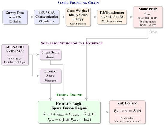
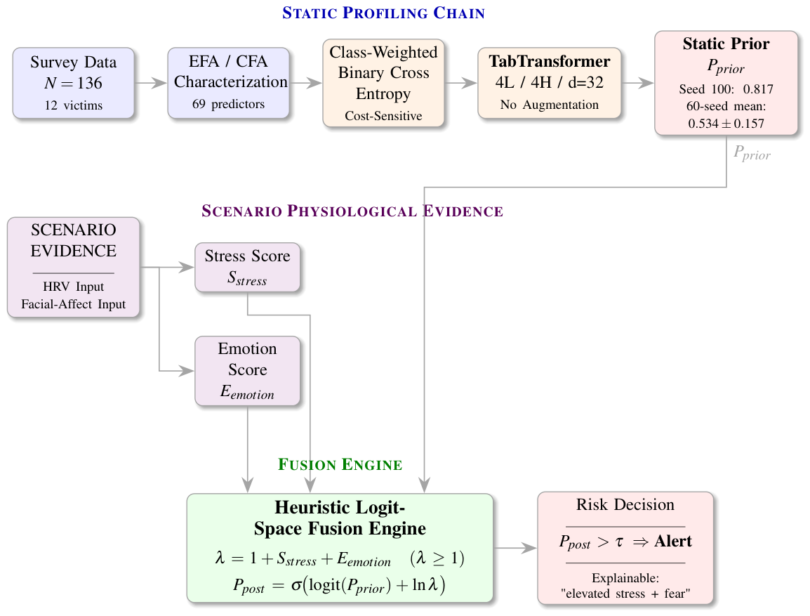
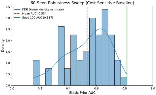
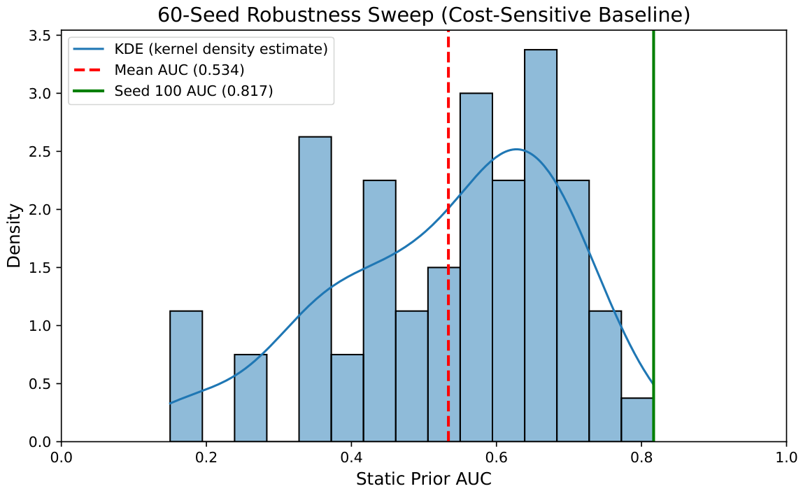
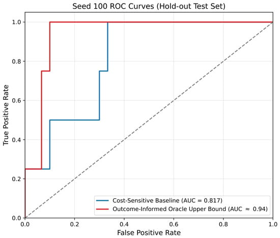
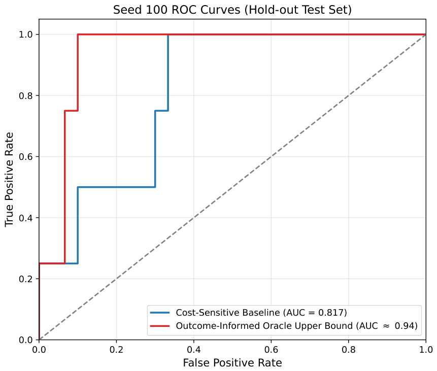
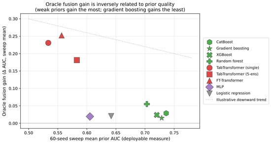
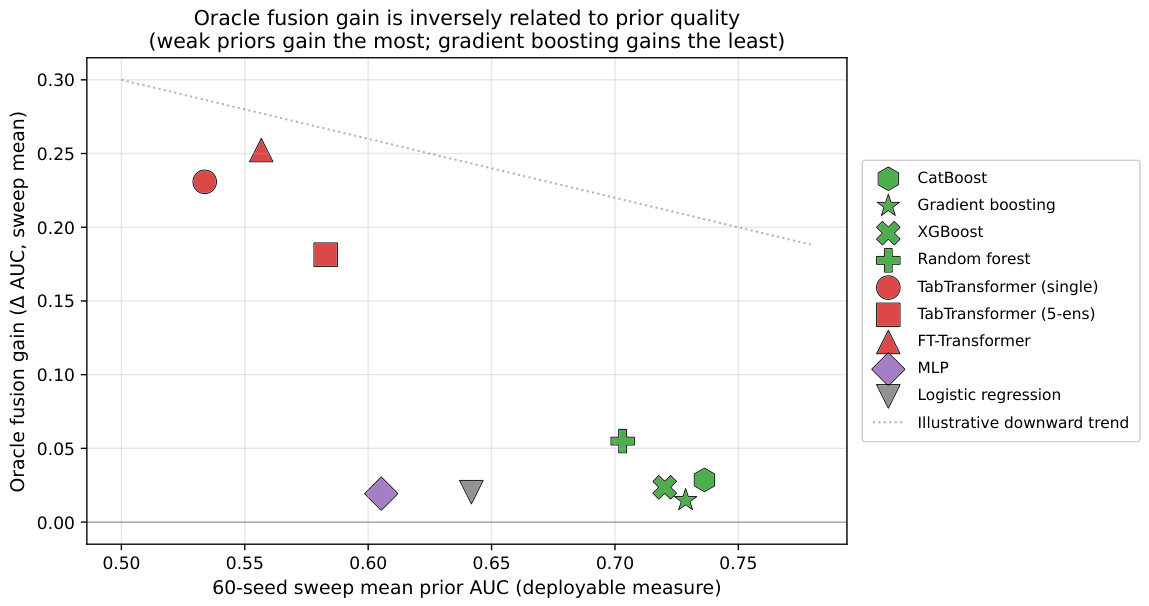
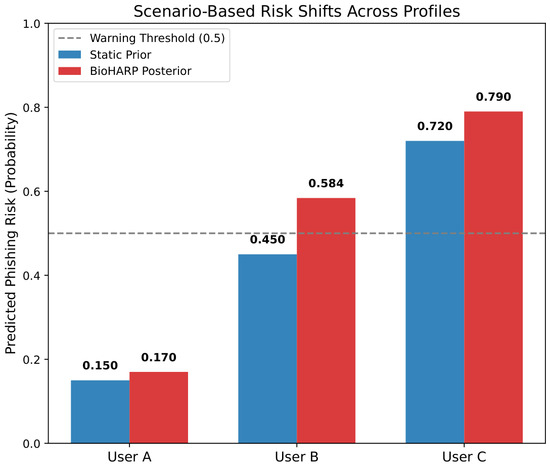
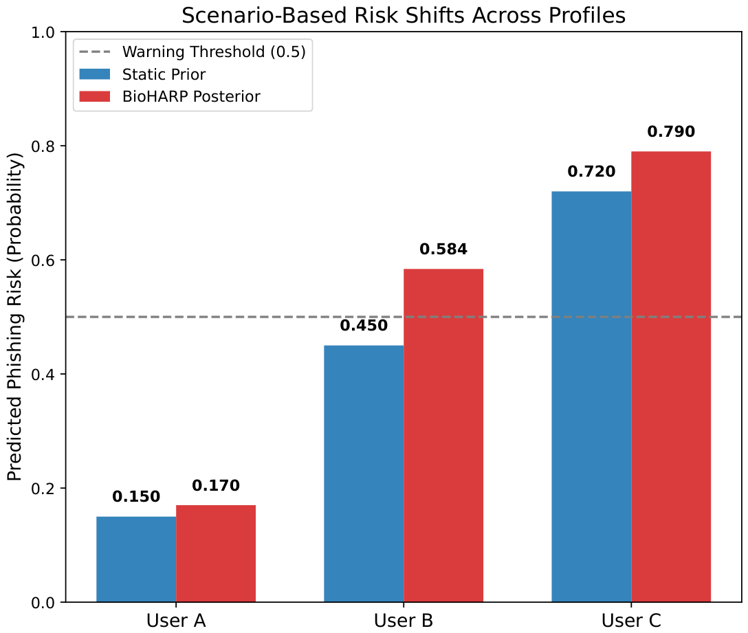

Disclaimer/Publisher’s Note: The statements, opinions and data contained in all publications are solely those of the individual author(s) and contributor(s) and not of MDPI and/or the editor(s). MDPI and/or the editor(s) disclaim responsibility for any injury to people or property resulting from any ideas, methods, instructions or products referred to in the content. |
© 2026 by the authors. Licensee MDPI, Basel, Switzerland. This article is an open access article distributed under the terms and conditions of the Creative Commons Attribution (CC BY) license.