


Abstract
Extreme orbital thermal cycling and temperature-dependent clearance nonlinearity make it difficult to predict contact–impact, stick–slip, and bifurcation responses of flexible deployable space structures with sufficient stability, accuracy, and computational efficiency. An Adaptive Dissipation–Precision Coordinated Multi-Scale Implicit Integration Algorithm (ADPC-MSIIA) is proposed. First, an absolute nodal coordinate formulation (ANCF)-based thermo-mechanical clearance-joint model with thermal-viscosity-modified contact and frictional/impact heat feedback is established; second, a dual-time-scale implicit integration scheme with dual- stability–dissipation control and third-order compensation is developed; finally, numerical validation is performed using a linear single-degree-of-freedom (SDOF) benchmark, a temperature-dependent clearance impact oscillator, finite-element and published benchmark comparisons, and a deployable annular truss antenna case. Simulation results show that ADPC-MSIIA achieves a high-frequency spectral radius of , an effective convergence order of , a maximum contact force error of , and a reduction in the global cumulative error compared with the generalized- method. This study contributes to knowledge by linking temperature-driven clearance evolution, frictional heat feedback, and adaptive numerical dissipation within a unified framework for predicting non-smooth thermo-mechanical deployment dynamics of large flexible space structures with clearance joints.
1. Introduction
Deployable space structures, including large annular truss antennas, are required to maintain deployment accuracy and dynamic stability under severe orbital thermal cycling. During repeated transitions between extremely low and high temperatures, differential thermal expansion changes the clearance of revolute joints and modifies the local material, contact, and frictional properties. These effects can excite contact–impact events, stick–slip motion, high-frequency flexible vibration, transient heat generation, and bifurcation phenomena in flexible multibody systems. The resulting dynamics are difficult to predict because the thermal field evolves slowly, whereas contact and friction events occur over much shorter time scales. A central bottleneck is therefore the lack of a numerically stable, accurate, and efficient framework that can capture temperature-dependent clearance evolution, two-way thermo-mechanical feedback, and non-smooth contact switching in a unified manner.
Existing studies on deployable structures and clearance joints have established the physical importance of thermally induced joint nonlinearity. Large deployable antennas and related space mechanisms have been shown to experience pronounced thermal deformation and clearance variation under orbital temperature changes [1,2]. Thermo-mechanical coupling analyses further indicate that clearance joints may generate nonlinear contact, frictional impact, stick–slip responses, and transient heat transfer [3,4]. These works clarify the engineering origin of the problem and demonstrate that joint clearance cannot be treated as a purely geometric imperfection. However, many existing models still describe clearance, contact force, friction, and temperature evolution in a partially coupled or sequential manner. As a result, the feedback loop in which temperature changes the clearance and material properties, while frictional and impact dissipation modify the temperature field, remains insufficiently represented. This limitation motivates the need for a closed-loop thermo-mechanical clearance-joint model.
Time integration algorithms for structural and multibody dynamics have been widely developed, but their applicability to thermo-mechanical clearance systems remains limited. The Newmark- method provides a classical foundation for structural time integration, but its conditional stability makes it vulnerable to divergence when strong impact nonlinearities and contact discontinuities are present [5]. The Hilber–Hughes–Taylor- (HHT-) method introduces numerical dissipation and has been extended to index-3 differential-algebraic equations, time-varying system identification, real-time hybrid simulation, and soil–structure interaction [6,7,8,9]. Nevertheless, its dissipation and stability are governed by a limited parameter structure, which may overdamp low-frequency deployment motion while still failing to suppress all contact-induced high-frequency oscillations. The generalized- method improves modal damping control and has become a common choice for flexible multibody dynamics [10,11]; however, its second-order accuracy may lead to accumulated errors in long-duration orbital simulations, and its convergence can deteriorate near contact–separation switching. Therefore, conventional implicit schemes do not fully resolve the conflict among stability, accuracy, and high-frequency dissipation in non-smooth thermo-mechanical systems.
Recent advances in contact algorithms and high-order implicit schemes have improved selected aspects of nonlinear dynamic simulation. Yang et al. developed an efficient beam-in-beam large sliding contact method that reduces computational cost while maintaining contact accuracy [12]. Other studies on optimal implicit single-step methods, three-parameter formulations, and A-stable two-step schemes have enhanced dissipation controllability and stability properties [13,14,15,16]. These developments are valuable for structural dynamics and contact analysis, but they are generally not designed for systems in which a slowly varying thermal field continuously changes the clearance manifold and material parameters while fast contact events generate heat feedback. Consequently, even advanced integration schemes may still require additional mechanisms for dual-time-scale coupling, adaptive dissipation control, and event-resolved treatment of non-smooth clearance dynamics.
Multi-scale and reduced-order methods provide another route for improving computational efficiency in complex dynamic systems. Time-decomposition explicit methods and hybrid linear–nonlinear separation strategies have demonstrated that slow and fast responses can be treated on different temporal grids [17,18]. Model reduction for rotor-bearing systems and modified harmonic balance methods for dual-rotor-casing dynamics further show that response decomposition can reduce the computational burden of nonlinear vibration analysis [19,20]. Parallel solution strategies, such as block Gaussian elimination for flexible multibody systems and hybrid time-domain discontinuous Galerkin methods, have also been used to alleviate large-scale computational bottlenecks [21,22]. However, these methods usually emphasize efficiency or frequency-domain representation rather than the simultaneous preservation of contact-event accuracy, thermal feedback consistency, and numerical robustness across discontinuous state transitions. Thus, multi-scale efficiency alone is insufficient for thermo-mechanical clearance joints unless it is combined with a switching-aware implicit integration strategy.
Thermo-mechanical discretization, friction modeling, and clearance-induced instability studies have provided important modeling components, but they remain fragmented for the present application. Hybrid high-order methods with Nitsche-type contact enforcement, adaptive isogeometric phase-field models, and monolithic thermo-mechanical formulations with hyperbolic heat conduction highlight the importance of tightly coupled field equations and reduced splitting errors [23,24,25]. Multi-physics validation studies on segmented tire molds and data-driven thermal analyses further confirm the relevance of two-way thermal–mechanical feedback [26,27]. For clearance systems, investigations of assembly robots with three-dimensional revolute clearances and dissipative contact in biped walkers demonstrate that friction and clearance modeling strongly affect stability prediction [28,29]. Failure analyses of aero-engine inter-shaft bearings and elastic ring dampers also identify clearance as a major source of premature wear, bifurcation, and chaotic response [30,31,32,33]. Although these studies offer useful contact, thermal, and stability modeling concepts, they do not provide an integrated framework for flexible deployable space structures with temperature-dependent clearance joints, partial-slip frictional heating, and moving discontinuity manifolds.
Based on the above critical assessment, three knowledge gaps can be identified. First, a closed-loop thermo-mechanical model is still needed to represent temperature-dependent clearance evolution, temperature-sensitive material/contact properties, and frictional/impact heat feedback within the same flexible multibody formulation. Second, existing implicit integration algorithms do not simultaneously provide full-spectrum stability, controllable high-frequency dissipation, high-order accuracy, and robust convergence for strong contact nonlinearities. Third, current multi-scale approaches do not adequately resolve the coupled dual-time-scale response in which slow thermal evolution interacts with fast stick–slip and contact–impact events on a time-varying clearance manifold. These gaps indicate that an effective solution should combine thermo-mechanical clearance modeling, adaptive multi-scale integration, independent stability–dissipation regulation, and non-smooth event handling in one consistent numerical framework.
An Adaptive Dissipation–Precision Coordinated Multi-Scale Implicit Integration Algorithm (ADPC-MSIIA) is proposed in this study. The new contribution to knowledge lies in the integration of an absolute nodal coordinate formulation (ANCF)-based thermo-mechanical clearance-joint model, a thermal-viscosity-modified contact/friction law with frictional and impact heat feedback, an asymptotic dual-time-scale decomposition, a dual- stability–dissipation control strategy, a third-order compensation scheme, and a self-starting substep iteration with arc-length continuation for contact switching and bifurcation tracking. In Section 2, a theoretical framework for thermo-mechanical gap dynamics in three-dimensional clearance joints is established, including temperature-dependent kinematics, material properties, partial-slip contact, augmented friction, embedded switching dynamics, and Poincaré mapping. In Section 3, the ADPC-MSIIA formulation is developed, including the three-layer architecture, dual-time-scale decomposition, dual- parameter control, third-order accuracy compensation, substep iteration, and convergence analysis. In Section 4, numerical validation and engineering application are performed through a linear single-degree-of-freedom benchmark, a temperature-dependent clearance impact oscillator, finite-element and published benchmark comparisons, and a deployable annular truss antenna case. In Section 5, the main conclusions are summarized, and future extensions are discussed.
2. Theoretical Modeling of Thermo-Mechanical Gap Dynamics in 3D Clearance Joints
This section develops a unified theoretical framework for the coupled thermo-mechanical response of three-dimensional revolute clearance joints in deployable space structures subjected to extreme orbital thermal cycling. The formulation builds upon the absolute nodal coordinate formulation (ANCF) for flexible multibody dynamics. It extends the original framework through a consolidated set of enhancements. First, a temperature-dependent kinematic and material description is introduced. Second, a refined normal and tangential contact model is adopted. This model incorporates partial-slip and thermal clearance evolution. Third, the friction law is augmented. It includes rising static friction and an Arrhenius-type thermal viscosity. Fourth, a discontinuous dynamical systems representation is employed. This representation features an explicitly time-varying switching manifold. Finally, a fully coupled thermo-mechanical governing system is established. The system embeds the switching dynamics directly within the ANCF equations. Subsequently, the Poincaré mapping technique is employed to analyze the constructed framework, so as to identify the reference point trajectories under periodic on-orbit thermal cycling conditions.
2.1. Unified Kinematic Thermo-Constitutive Contact and Discontinuous System Formulation
Figure 1 illustrates the unified theoretical modeling framework for the three-dimensional revolute clearance joints subjected to orbital thermal cycling, which integrates the absolute nodal coordinate formulation (ANCF)-based kinematic description, temperature-dependent material constitutive relations, a normal contact–impact model with hysteresis damping, a partial-slip tangential friction model considering thermal viscosity and rising static friction, Filippov-type discontinuous dynamical representation with a time-varying switching manifold, and fully coupled thermo-mechanical governing equations. It systematically depicts the two-way thermo-mechanical interaction mechanism, where the temperature field alters the joint clearance and material properties, and the contact–friction–impact events generate frictional heat that feeds back to the thermal field, forming the closed-loop thermo-mechanical coupled dynamic system for flexible multibody deployable space structures.
Figure 1.
Kinematic and thermo-constitutive modeling framework for 3D temperature-dependent clearance revolute joints in flexible multibody deployable space structures.
The position field of an arbitrary material point within a three-dimensional ANCF beam element is interpolated as
where denotes the local material coordinates, is the shape function matrix constructed from cubic Hermite polynomials, and is the global absolute nodal coordinate vector containing both position and gradient degrees of freedom. To eliminate mesh-mismatch errors in multi-physics coupling, the temperature field is interpolated using the identical shape functions:
where is the element nodal temperature vector.
Figure 2 displays the temperature-dependent variations in six key thermophysical and mechanical properties—density, Young’s modulus, Poisson’s ratio, the thermal expansion coefficient, thermal conductivity, and specific heat capacity—for five widely used aerospace materials: Ti-6Al-4V, AISI 304 stainless steel, Al 7075-T6, Al 6061-T6, and carbon fiber reinforced polymer (CFRP), over the orbital temperature range of to . These curves are generated from the reference values and temperature coefficients listed in Table 1, based on the constitutive relations given in Equation (3). In our work, Ti-6Al-4V and AISI 304 are employed for the pin and lug of the single revolute clearance hinge benchmark (Section 4.3.2), while Al 7075-T6, Al 6061-T6, and CFRP provide a general thermophysical database for truss members and flexible components of large deployable antennas. The actual truss members of the deployable annular truss antenna (Section 4.4.1) are made of 2A12 aluminum alloy, whose properties are also provided in Table 1. The results show that thermal conductivity and specific heat capacity are strongly temperature-sensitive, whereas density remains nearly constant, supplying essential constitutive parameters for thermo-mechanically coupled dynamic modeling of deployable structures with clearance joints.
Figure 2.
Temperature−dependent thermophysical and mechanical properties of typical aerospace structural materials.
Table 1.
Thermophysical and mechanical properties of aerospace structural materials at 25 °C and their temperature coefficients.
In a clearance joint, the two contacting components may be fabricated from different materials and therefore possess distinct temperature-dependent characteristics. For each material, the temperature-dependent density , Young’s modulus , Poisson’s ratio , thermal expansion coefficient , thermal conductivity , and specific heat capacity are described by the following constitutive relations:
where is the reference temperature. The reference values and thermal coefficients for all materials are listed in Table 1. These temperature-dependent properties govern the mass matrix , elastic stiffness matrix , structural damping matrix , and thermal load vector appearing in the coupled governing equations.
The temperature coefficients used in Equation (3) are , , , , , , and . These coefficients are applicable to all metallic materials listed in Table 2; the corresponding coefficients for CFRP differ slightly and are provided separately in the revised manuscript. All parameters are sourced from authoritative aerospace material handbooks and the published literature to ensure the accuracy and reproducibility of the numerical simulations.
Table 2.
Three-layer architecture specifications of the ADPC-MSIIA algorithm.
The radial clearance of a revolute joint is directly modified by the differential thermal expansion of the bushing (outer radius ) and the pin (outer radius ). Including quadratic nonlinearity in addition to the linear thermal expansion, the instantaneous clearance is expressed as
where is the nominal room-temperature clearance, and are the temperature-dependent thermal expansion coefficients of the bushing and pin materials, respectively, and accounts for nonlinear geometric effects at extreme temperatures.
Let the gap function be defined as
where is the relative position vector between the pin and bushing surfaces, and contact occurs when . The normal contact pressure within the contact annulus is given by the Hertzian solution for cylindrical contact:
where is the instantaneous contact radius, and is the normal contact force. The latter is determined from the indentation depth , using the modified Hertz law with hysteresis damping:
with temperature-dependent contact stiffness computed from the effective modulus and effective radius .
The tangential contact description previously relied on a regularized Coulomb law, assuming either full stick or full slip over the entire contact area. Here we adopt the classical Cattaneo–Mindlin–Jäger theory, adapted for a temperature-dependent conformal cylindrical contact, in order to resolve the partial-slip annulus and stick-zone evolution. Within the contact annulus, the tangential stress distribution is expressed as the difference between two normal pressure distributions corresponding to the contact radius and the stick radius :
where is the temperature-dependent friction coefficient, denotes the normal pressure for a contact radius a, and the Heaviside factor ensures that the stress vanishes outside the contact region. The stick radius is determined by the global tangential force balance
where is the total tangential force obtained by integrating the tangential stress over the contact area:
The tangential displacement within the stick zone is uniform and given by
where is the normal approach corresponding to a contact radius a, and is the temperature-dependent equivalent shear modulus. The slip velocity is then
with denoting the relative angular velocity between the pin and bushing.
To better capture the thermally activated stick–slip phenomenon observed in deployable masts, the friction law is further augmented with two additional mechanisms: rising static friction and thermal viscosity.
Rising Static Friction. The static friction coefficient depends on both the stick time (the duration of the current stick phase) and the local temperature, following the extended Kato model:
where and are the reference static and kinetic friction coefficients at , and are their respective temperature coefficients, and and m are stick-time sensitivity parameters. The stick time itself is temperature-dependent, reflecting enhanced molecular mobility at elevated temperatures:
with denoting the reference stick time at and denoting the temperature coefficient.
Thermal-Viscosity Damping. During the slip phase, an additional velocity-dependent viscous term is introduced to account for the thermal softening of the contact interface. The thermal-viscosity coefficient follows an Arrhenius-type law:
where is the reference viscosity at , is the activation energy, R is the universal gas constant, and is the absolute temperature in Kelvin.
The complete tangential force in the slip regime (, where is a small threshold velocity) is then
where is the instantaneous contact area. In the stick regime , the friction force is bounded by the static friction capacity:
To obtain a rigorous mathematical classification of motion states at the clearance boundary—particularly to distinguish a simple impact from sustained thermally induced sliding—the joint dynamics are reformulated as a Filippov discontinuous system with an explicitly time-varying switching manifold. We define the extended state vector as
where are the ANCF nodal coordinates, are the corresponding velocities, and are the nodal temperatures. The switching manifold for the ith clearance joint is defined as
where is the relative radial penetration depth. Because the clearance varies with temperature, the manifold moves through the phase space with velocity .
The state space is partitioned into two regions: the separation region , where the joint is free of contact, and the contact region , where normal and tangential contact forces are active. The vector fields in these two regions are denoted by and , respectively, and are obtained from the coupled ANCF dynamic equations with the gap force vector set to zero in and fully active in . The explicit forms of and are provided in Section 2.2.
To classify the trajectory behavior at the switching manifold, the G-function formalism is employed. The unit normal vector to the manifold is
The zero-order G-function, which measures the projection of the vector field onto the manifold normal relative to the manifold motion, is defined as
The first-order G-function, required for grazing bifurcation detection, is
The motion at the clearance boundary is classified according to the signs of and : crossing motion (impact) when ; sliding motion (thermally induced stick–slip) when ; and grazing motion when with . The inclusion of in Equation (21) accounts for the motion of the clearance boundary due to thermal expansion, an effect absent in traditional clearance-joint models.
2.2. Fully Coupled Governing Equations with Embedded Switching Dynamics
Figure 3 illustrates the core numerical procedure of the adaptive multistep half-implicit algorithm (ADPC-MSIIA) for solving thermo-mechanical coupled discontinuous dynamics of clearance revolute joints. Upon detecting a contact event, the algorithm first refines the time step via successive bisection and interpolation to locate the exact switching instant , where the thermal state , temperature-dependent clearance , friction coefficients , , and thermal viscosity are updated. G-functions are then evaluated to classify the motion state (separation, crossing, or sliding), and the corresponding Filippov vector field , , or is applied. Subsequently, the friction state (stick/slip) is assessed: for slip, the enhanced thermal friction law is activated, and frictional heat generation is computed; for stick, the static friction criterion is checked, and the stick time is tracked to capture the rising static friction effect. The state variables are then advanced within the refined substep using ADPC-MSIIA, and the thermal state change is verified to ensure the consistency of thermally coupled parameters. The process terminates when the original time step is completed, enabling accurate and efficient integration of the stiff, discontinuous, and thermally coupled contact–friction dynamics in flexible multibody deployable structures.
Figure 3.
Flowchart of the thermally coupled adaptive time-stepping integration algorithm for Filippov-type discontinuous contact–friction systems.
The governing equations for the coupled thermal and mechanical fields are derived by embedding the vector fields and of the discontinuous system within the ANCF framework. The resulting semi-discretized system constitutes a closed-loop formulation with two-way thermo-mechanical coupling.
Mechanical Field. The dynamic equilibrium equation in region , , is
where is the temperature-dependent mass matrix, is the Rayleigh damping matrix, is the elastic stiffness matrix, is the thermal load vector, represents external deployment forces and orbital perturbations, and is the generalized force vector from all clearance joints. Specifically,
where is given by Equation (7), is given by the enhanced friction model of Equations (16) and (17), and , are the ANCF Jacobian matrices that transform contact forces to generalized coordinates.
Equation (23) can be cast into first-order form to define the vector fields introduced in Section 2.1:
where is obtained from the thermal field equation discussed below.
Thermal Field. The transient heat conduction equation, including frictional and impact heat sources, is discretized as
where is the thermal damping (heat capacity) matrix, is the thermal conductivity matrix, accounts for absorbed orbital radiation, and is the nodal heat source vector from frictional sliding and impact dissipation.
The refinement in the present model lies in the computation of . Instead of assuming full slip, the frictional heat flux is evaluated using the slip velocity from the partial-slip solution (Equation (12)) and integrated over the actual slip annulus :
The heat is partitioned between the pin and bushing according to their thermal effusivities :
The distributed heat fluxes are then integrated over the element domains to form the consistent nodal heat source vector . This spatial refinement ensures that the thermal feedback accurately reflects the localized heating within the slip annulus.
Two-Way Coupling and Sliding Vector Field. Equations (23) and (26) constitute a closed-loop system of differential-algebraic equations. The temperature field influences the mechanical response through the temperature-dependent material properties (Equation (3)), the thermal load , and the clearance size . Conversely, the mechanical motion generates frictional and impact heat, which feeds back into the thermal field via .
During sliding motion on the switching manifold , the trajectory is governed by the Filippov sliding vector field , which is a convex combination of and :
with the scalar chosen such that . Using Equation (21), this condition yields
The sliding dynamics thus incorporate both the thermal drift of the clearance boundary and the coupled thermo-mechanical response of the structure.
The system exhibits a dual-time-scale characteristic: the temperature field evolves slowly with a time scale , while the stick–slip vibrations and contact–impact transients occur on a fast time scale . This separation motivates the multi-scale integration algorithm developed in Section 3.
2.3. Poincaré Mapping for Periodic Thermo-Mechanical Orbits
To analyze the long-term deployment dynamics and identify stable periodic orbits under thermo-mechanical coupling, a Poincaré mapping framework is established based on the coupled system derived in Section 2.1 and Section 2.2. A Poincaré section is chosen at a fixed deployment angle (e.g., the fully stowed or fully deployed configuration). The Poincaré map is defined as the evolution of the extended state vector (Equation (18)) from one intersection with to the next.
The map is decomposed into a composition of elementary mappings corresponding to the different contact phases encountered during one orbital thermal cycle, incorporating the vector fields defined in Equations (25) and (29):
where propagates the state through the separation region , , governed by the vector field (Equations (25) with ); propagates the state through the contact region , , governed by the vector field (Equations (25) with the enhanced contact forces of Equations (7), (16) and (17)); propagates the state along the switching manifold during sliding motion, governed by the Filippov sliding vector field (Equation (29) with from Equation (30)); evolves the temperature field over the time interval, accounting for the slow thermal dynamics described by Equation (26).
Fixed points of the Poincaré map, , correspond to periodic thermo-mechanical deployment orbits. The stability of a periodic orbit is determined by the eigenvalues (Floquet multipliers) of the Jacobian matrix evaluated at the fixed point. If all eigenvalues lie within the unit circle, the orbit is asymptotically stable.
The Poincaré map offers a systematic tool to locate periodic orbits and assess their stability under the fully coupled thermo-mechanical framework of Section 2.1 and Section 2.2. Going beyond the time-domain parametric studies presented in some companion works, this approach enables bifurcation analyses (e.g., period-doubling, grazing bifurcations) that are crucial for predicting deployment reliability under thermal cycling. The practical computation of and its Jacobian is addressed in Section 4, where the multi-scale integration scheme is coupled with a shooting algorithm.
3. The Proposed ADPC-MSIIA Algorithm
This section presents the complete theoretical derivation of the ADPC-MSIIA, specifically tailored for the coupled thermo-mechanical system with three-dimensional clearance joints developed in Section 2. The algorithm addresses the dual-time-scale nature of the problem—slow thermal evolution coupled with fast impact-induced vibrations and stick–slip transients—while rigorously handling the discontinuous dynamics at the time-varying switching manifold . The derivation encompasses a three-layer architecture, a systematic dual-time-scale decomposition of the fully coupled governing Equations (23) and (26), a dual- stability–dissipation decoupling control, a third-order accuracy compensation scheme, a self-starting substep iteration with arc-length continuation for non-smooth events, and a rigorous global convergence proof.
The complete implementation flow of the proposed multi-timescale thermally coupled adaptive integration framework, built upon the ADPC-MSIIA algorithm for solving the thermo-mechanical coupled DAE system in Section 2.2, is summarized below and illustrated in Figure 4.
Figure 4.
Implementation flowchart of the ADPC-MSIIA algorithm.
Step 1: Initialization.
Construct the ANCF model of the deployable structure as per Section 2.1.
Initialize the nodal coordinate vector , velocity , and temperature field from the stowed configuration.
Table 3.
Recommended dual- parameter sets for different deployment scenarios.
Table 4.
Optimization results of the third-order compensation coefficient .
Step 2: Slow Field Solution.
Solve the coupled slow Equations (36) and (37) using a BDF2-based monolithic Newton–Raphson iteration.
The time-averaged gap forces and heat source are computed by sampling the fast-field response over one representative cycle or using a precomputed emulator.
Step 3: Fast Field Prediction.
With the updated slow fields and acting as frozen parameters, advance the fast fields and using the ADPC-MSIIA scheme (42)–(45) with time step .
Monitor the gap function for contact detection.
Step 4: Substep Iteration and Switching Correction.
If a contact event is detected, refine the step via Equation (48) to locate the exact switching instant .
Evaluate the G-functions (Equations (21) and (22)) to classify the post-impact motion. Apply the appropriate vector field , , or (29) within each substep.
Step 5: Arc-Length Continuation (if required).
If a bifurcation is anticipated (e.g., onset of stick–slip), augment the slow-field system with the arc-length constraint (49) to traverse limit points and track solution branches.
Step 6: Multi-Field Feedback.
Update the fast temperature field and, upon cycle completion, provide the time-averaged heat source for the next slow-field step.
Step 7: Convergence and Termination Check.
If the total simulation time is reached, terminate the calculation and output the deployment history. Otherwise, return to Step 2 for the next slow time step.
3.1. Three-Layer Architecture of ADPC-MSIIA
The ADPC-MSIIA algorithm is designed with a three-layer architecture to address the specific challenges of thermo-mechanical coupled dynamics with clearance nonlinearity, as summarized in Table 2.
3.2. Dual-Time-Scale Decomposition of the Thermo-Mechanical Coupled System
The governing equations presented in Section 2.2—the mechanical equilibrium Equation (23), its equivalent state-space form (25), and the transient heat conduction Equation (26)—together constitute a closed-loop system characterized by fundamentally disparate time scales. For typical deployable space structures, the thermal diffusion time scale is on the order of , whereas the stick–slip vibrations and contact–impact transients occur on a fast time scale . This separation motivates the introduction of a small parameter , defined as the ratio of the fast to the slow characteristic times, typically .
Two independent time variables are introduced:
The extended state vector of Equation (18) is expanded in an asymptotic series with respect to :
where subscript 0 denotes slow-varying components that depend solely on , and subscript 1 denotes fast-varying fluctuations that depend on both and . The time derivative operators transform according to the chain rule:
Substituting the expansions (34) and the derivative operators (35) into the coupled Equations (23) and (26), and collecting terms of like powers of , yields a hierarchical system of decoupled slow-varying and fast-varying governing equations.
3.2.1. Slow-Varying Governing Equations
Figure 5 depicts the iterative solution procedure for the slow-varying thermal subsystem, which forms a core part of the multi-timescale thermo-mechanical coupling framework. Starting with an initial guess for the generalized coordinate state and temperature field , the algorithm evaluates the residual vector of the governing thermal equations (Equations (36) and (37)). If the residual norm exceeds the predefined tolerance, the tangent system is solved using the BDF2 (Backward Differentiation Formula of order two) combined with the Newton–Raphson method to obtain the correction term , which is then used to update and . The iteration continues until the residual converges to within the tolerance. Upon convergence, the time-averaged contact gap force and frictional heat source are computed via the fast-field emulator, and the solution returns to the main multi-timescale integration loop. This procedure ensures stable and accurate resolution of the slow thermal dynamics while incorporating the averaged effects of the fast contact–friction events.
Figure 5.
Flowchart of the slow-field thermal solution module with the BDF2–Newton–Raphson iteration.
At the leading order , the mechanical equilibrium and thermal conduction equations describe the quasi-static evolution of the structure under the time-averaged influence of the fast contact dynamics. The slow mechanical equation is obtained by substituting the expansion into Equation (23) and applying the fast-time averaging operator defined in Equation (38) below:
where accounts for geometric nonlinearities inherent in the ANCF formulation. The slow thermal equation is similarly derived from Equation (26):
in which the fast-time averaging operator is defined as
with being the characteristic period of the fast vibrations. The averaged gap force vector incorporates the time-averaged contributions of the normal contact force (7) and the enhanced tangential force (16) and (17) over one fast oscillation cycle. Likewise, is the time-averaged frictional heat source computed from the partial-slip solution (27) and the effusively-based partition (28).
3.2.2. Fast-Varying Governing Equations
At the next order , the equations govern the fast transient dynamics of the vibration and stick–slip phenomena, with the slow-varying fields and acting as slowly varying parameters. The fast mechanical equation reads
where the fast-fluctuating components are defined as . In particular, captures the deviation of the instantaneous contact forces from their time-averaged values, and it is precisely this term that drives the stick–slip transitions governed by the switching manifold of Equation (19). The fast thermal equation is
where represents the rapidly fluctuating frictional heat generation during partial-slip events.
Equations (36), (37), (39) and (40) form the basis for the multi-scale integration strategy: the slow fields are advanced with a large time step , while the fast fields are resolved within each slow step using a smaller time step and the specialized integration scheme detailed in Section 3.3, Section 3.4 and Section 3.5.
Figure 6 visualizes the bidirectional thermo-mechanical coupling process across successive iterations, showing the evolution of three core fields: (1) the slow temperature field , where a localized hot spot forms due to accumulated frictional heat generation; (2) the fast displacement field u, which is statically balanced using a temperature-dependent Young’s modulus , leading to larger deflections in the heated region; and (3) the fast velocity field v, whose magnitude directly determines the frictional heat source term . The bottom caption confirms that the mapping satisfies the contraction condition , proving the convergence and stability of the multi-timescale iteration scheme. The results clearly demonstrate the closed-loop interaction: the temperature field modifies material stiffness and structural deformation, while the resulting mechanical motion generates frictional heat that feeds back to the thermal field.
Figure 6.
Multi-timescale coupled evolution of the slow temperature field and fast mechanical fields over the iteration loop.
3.3. Dual- Parameter Stability–Dissipation Decoupling Control
Traditional time integration methods for structural dynamics, such as the generalized- scheme, employ a single parameter (or a pair of linked parameters) to control both numerical stability and high-frequency dissipation. For strongly nonlinear systems with time-varying stiffness induced by thermal effects and contact switching, this coupling often leads to excessive low-frequency dissipation or insufficient damping of spurious high-frequency oscillations. To overcome this limitation, ADPC-MSIIA introduces two independent control parameters: the stability parameter and the dissipation parameter .
The method is applied to the semi-discrete fast-varying mechanical Equation (39), rewritten in the compact form
where the dependence on the slow time is temporarily suppressed for notational clarity. The weighted residual form of the algorithm over the fast time interval is constructed as
The algorithmic parameters and are mapped from the dual- parameters via the decoupled relations
where controls the spectral radius in the low-frequency range , ensuring to preserve the accuracy of rigid deployment motion and fundamental flexible modes; governs the numerical damping in the high-frequency range , ensuring rapid attenuation of spurious oscillations induced by contact discontinuities and numerical stiffness.
The displacement and velocity updates follow the standard Newmark formulas augmented with a third-order compensation coefficient . This unified update formulation remains unchanged for both smooth motion and collision-induced non-smooth responses. It achieves an ideal third-order error compensation effect when the system state maintains high-order continuity, while its theoretical third-order accuracy naturally degrades to the second-order level in collision and contact switching scenarios due to discontinuity of high-order state derivatives:
with the secondary parameters and given by
Recommended parameter sets for different deployment scenarios, determined through extensive numerical optimization, are listed in Table 3.
The unconditional stability of the ADPC-MSIIA integration scheme is rigorously established through spectral analysis of the linear single-degree-of-freedom (SDOF) model problem . The amplification matrix relating the state vector to its value at step n is constructed from the algorithmic Equations (42)–(44). The spectral radius determines stability: the scheme is unconditionally stable if and only if for all .
For the undamped case , the spectral radius as a function of the dimensionless frequency is obtained in closed form:
For the admissible parameter ranges and , the corresponding and from (43) satisfy . Consequently, the numerator in (46) is strictly less than or equal to the denominator for any , yielding over the entire frequency spectrum. The equality holds only in the limit , while for , the spectral radius asymptotically approaches a constant value , the specific numerical value of which is determined by the chosen parameter set as listed in Table 2. This completes the proof of unconditional stability.
3.4. Third-Order Accuracy Compensation Scheme
Comparing the third-order ADPC-MSIIA scheme with classical second-order methods is entirely justified: ADPC-MSIIA inherits the single-step implicit architecture, matrix assembly, and Newton–Raphson iteration of the generalized- family, ensuring nearly identical per step computational cost and a fair baseline for performance evaluation. Second-order generalized- methods are the de facto standard in both academic research and commercial software for thermo-mechanical analysis of deployable space structures with clearance joints. In long-duration orbital simulations spanning hundreds of thermal cycles, their local truncation error can accumulate to degrade clearance evolution and deployment kinematics predictions. ADPC-MSIIA addresses this limitation by introducing a third-order correction derived from the Taylor expansion of the state variables, thereby reducing global error without altering the underlying efficient solver structure, which offers clear practical benefits for multi-clearance deployable antenna engineering.
The exact Taylor expansion of the nodal coordinate at reads
The third derivative captures the time variation in the stiffness matrix induced by the slow temperature drift and instantaneous contact state transitions. Differentiating the fast dynamic Equation (39) with respect to yields an expression for in terms of the state variables and the rate of change in the contact forces. It is worth noting that this physical interpretation and continuous differential relation fail when abrupt collision-induced state jumps occur, which breaks the basic assumption of the above Taylor series derivation.
To avoid the computational expense of explicitly evaluating the third derivative, ADPC-MSIIA absorbs its effect into the Newmark updates through the compensation coefficient , as shown in Equation (44). The optimal value of is determined by minimizing the leading term of the local truncation error for a representative nonlinear oscillator with time-varying stiffness under smooth continuous motion conditions. Table 4 summarizes the performance metrics for various choices of , where the LTE is measured on a benchmark problem involving a thermally induced stick–slip transient with continuous state variation. The value achieves a measured convergence order of , which can realize nearly third-order numerical accuracy for displacement and velocity in smooth, strong nonlinear systems with time-varying stiffness.
Nevertheless, this ideal third-order accuracy cannot be maintained steadily in typical non-smooth systems featuring rigid collision, instantaneous contact separation, and constraint switching. In such discontinuous dynamic scenarios, the discontinuity of high-order state derivatives invalidates the full effect of the compensation term, and the practical convergence order of the scheme naturally degenerates to the second-order level. To compensate for this accuracy degradation in non-smooth regions, additional local substep iteration and arc-length continuation strategies are adopted cooperatively in the overall algorithm framework.
3.5. Self-Starting Substep Iteration with Arc-Length Continuation
The presence of the time-varying switching manifold defined in Equation (19) introduces discontinuities in the vector fields and whenever the trajectory crosses . Moreover, the G-function criteria (21) and (22) determine whether a crossing results in a simple impact or transitions into a sliding phase along the manifold. To accurately resolve these events and to track the associated bifurcations, ADPC-MSIIA incorporates a self-starting substep iteration scheme coupled with an arc-length continuation procedure.
Figure 7 illustrates the arc-length continuation module, which is designed to trace solution branches and capture bifurcation or limit-point behavior in the multi-timescale thermo-mechanical system. Starting with the definition of the continuation parameter (e.g., orbit-averaged temperature T or initial clearance ), the slow-field governing system is augmented with the arc-length constraint equation (Equation (49)). The augmented system is solved using the bordered Newton–Raphson method, iterating until the residual converges. Upon convergence, the state variables are updated, and a check is performed to detect whether a limit point or bifurcation point has been encountered. If such a critical point is detected, the continuation step size is adjusted, or the solution branch is switched to maintain numerical stability and track the full solution manifold. The procedure terminates by returning to the main multi-timescale integration flow, ensuring the framework can resolve complex nonlinear dynamic behaviors induced by thermal and clearance effects.
Figure 7.
Flowchart of the arc-length continuation procedure for capturing bifurcation and limit-point behavior.
3.5.1. Self-Starting Mechanism
At the initial time step, the acceleration is not known a priori. ADPC-MSIIA adopts a predictor–corrector self-starting strategy:
Assume and compute a first prediction using (44) with temporarily.
Substitute the predicted state into the dynamic equilibrium Equation (39) to solve for a corrected acceleration .
Iterate the corrector step until the residual norm satisfies .
This approach avoids the need for an explicit initial acceleration computation and preserves the formal order of accuracy from the very first step.
3.5.2. Substep Refinement for Contact–Separation Switching
During the fast-field integration, the algorithm monitors the gap function from Equation (5). A sign change indicates that the trajectory has crossed the switching manifold within the current time step . To capture the exact switching instant and to avoid numerical oscillations arising from force discontinuities, the time step is recursively refined:
until the relative change in the estimated crossing time falls below a prescribed tolerance. Within each substep, the appropriate vector field— for , for , or the Filippov sliding field from Equation (29) when sliding is detected via the G-function criterion—is employed. This event-driven refinement guarantees that the normal impact law (7) and the enhanced tangential friction model ((16) and (17)) are applied precisely at the contact interface, thereby conserving energy and momentum to within the algorithm’s truncation error.
3.5.3. Arc-Length Continuation for Bifurcation Tracking
The thermo-mechanical deployment dynamics governed by Equations (36)–(40) can exhibit complex nonlinear bifurcations, including the onset of stick–slip limit cycles and period-doubling cascades as the clearance varies along the orbit. To trace solution branches past turning points and to accurately locate bifurcation critical points, an arc-length continuation constraint is appended to the nonlinear algebraic system arising from the slow-field solution step:
where is a chosen continuation parameter (e.g., the orbit-averaged temperature or the nominal clearance ), and is the prescribed arc-length step size. The augmented system is solved using a monolithic Newton–Raphson procedure with a bordering algorithm. This enables the ADPC-MSIIA framework to seamlessly traverse limit points and to compute the Poincaré map fixed points introduced in Section 2.3 as part of a bifurcation analysis.
3.6. Global Convergence and Symplectic Property Discussion
The global convergence of the iterative coupling between the slow thermal field and the fast mechanical response within the ADPC-MSIIA framework is established using the contraction mapping theorem. The iteration over one slow time step is formulated as a fixed-point mapping acting on the slow temperature field , with the fast-field dynamics treated as a functional of the temperature-dependent material and contact parameters. A strict contraction property of guarantees a unique thermo-mechanical equilibrium state for each slow time increment, ensuring algorithmic robustness in long-duration simulations.
The contraction condition is verified by bounding the sensitivity of the averaged frictional heat source appearing in the slow thermal equation (Equation (37)) with respect to . Using the partial-slip heat flux expression (27) together with the temperature-dependent friction coefficient (13), the gradient satisfies
An analogous bound holds for the nonlinear structural stiffness , whose temperature sensitivity is governed by the thermal expansion coefficient given in Equation (3):
The Lipschitz constant L of the composite mapping is then bounded by . For a representative slow time step , this gives , establishing the mapping as a strict contraction in the supremum norm. Hence the iteration possesses a unique fixed point and converges exponentially to the thermo-mechanical solution, providing a theoretical guarantee of stability and accuracy even for orbital simulations involving thousands of thermal cycles.
Concerning the symplectic property, ADPC-MSIIA belongs to the generalized- family and operates with an asymptotic spectral radius ; by definition, it cannot preserve the symplectic 2-form . This non-symplectic character is a direct consequence of the deliberately introduced high-frequency numerical dissipation, which is indispensable for suppressing spurious oscillations excited by repeated contact–impact events in clearance joints. Notably, the loss of symplecticity is also a fundamental limitation of odd-order integration methods—Hairer et al. [34] proved that no odd-order method can be symplectic—leading to long-term energy drift and failure to conserve phase-space volume. In ultra-long orbital simulations spanning hundreds or thousands of thermal cycles, such drift could induce artificial orbital decay or expansion if left unaddressed.
For the non-conservative, non-smooth thermo-mechanical systems considered in this work, purely symplectic integrators (e.g., the Newmark- method with ) are inherently unsuitable because they lack any mechanism to damp contact-induced high-frequency noise, causing non-physical force oscillations and potential instability, as evidenced by the maximum contact force error reported in Section 4.3. Recent semi-implicit symmetric methods, D-methods, and multistep semi-implicit integrators [35,36,37,38] attempt to reconcile partial symplecticity with limited dissipation, yet their application to systems with strong clearance nonlinearities and dual-time-scale thermo-mechanical coupling remains an open challenge. State-of-the-art symmetric schemes, such as SEABM and SIABM, improve long-term stability by preserving time reversibility and reducing energy drift. However, these methods generally entail more complex implementations and higher computational cost than generalized- algorithms—especially in systems exhibiting frequent contact state transitions—and often require specialized modifications to maintain their geometric properties across contact–separation discontinuities.
To mitigate the potential energy drift while retaining the core advantages of ADPC-MSIIA (third-order accuracy, efficient contact handling, and computational cost comparable to second-order generalized- methods), we have incorporated a periodic energy renormalization strategy tailored for orbital deployable antenna simulations. This strategy applies an energy correction at intervals corresponding to the orbital period, adjusting the system energy to match the theoretical Hamiltonian derived from the slow thermal drift model. It effectively counteracts artificial energy accumulation while preserving the fidelity of fast-scale contact–impact dynamics, keeping the energy drift within an acceptable range for engineering applications.
ADPC-MSIIA therefore sacrifices symplectic structure in a controlled manner to achieve a practical balance between long-term accuracy and short-term stability, making it particularly well suited for engineering analysis of deployable space structures over typical orbital thermal cycles. Table 5 presents a quantitative comparison among ADPC-MSIIA (with energy renormalization), SEABM, and SIABM on a benchmark thermo-mechanical clearance-joint system subjected to 100 thermal cycles, illustrating the trade-offs between geometric preservation, contact accuracy, and computational efficiency.
Table 5.
Quantitative comparison of ADPC-MSIIA (with energy renormalization), SEABM, and SIABM for thermo-mechanical clearance-joint system.
Future work will explore hybrid integrators that combine symplectic structure preservation during smooth dynamic phases with the proposed dissipation control mechanism at contact–impact events, aiming to further enhance performance for ultra-long-term orbital simulations. Additionally, we plan to conduct a systematic comparison with other higher-order symplectic composition methods (e.g., those based on the Suzuki–Yoshida decomposition [4]) to further improve the geometric preservation capability of the algorithm without sacrificing contact handling accuracy.
4. Numerical Validation and Engineering Application
This section presents a comprehensive numerical validation of the proposed ADPC-MSIIA algorithm. The assessment proceeds in three successive stages. First, a linear single-degree-of-freedom system is employed to examine the unconditional stability, convergence order, and high-frequency dissipation characteristics against several classical and improved implicit time integration methods, including Newmark-, Hilber–Hughes–Taylor- (HHT-), generalized-, and the improved Hilber–Hughes–Taylor- (improved HHT-). Second, a strongly nonlinear clearance impact oscillator with a temperature-dependent joint gap is simulated to evaluate accuracy, computational efficiency, and robustness under contact–separation discontinuities and frictional dissipation. Third, the validated algorithm is applied to an engineering-scale model of a large deployable annular truss antenna with multiple temperature-sensitive revolute clearance joints, where parametric bifurcation analyses and phase portraits are conducted to reveal the effects of orbital temperature, static and kinetic friction coefficients, and initial clearance sizes on the grazing bifurcation critical clearance and route-to-chaos. The performance metrics adopted throughout the evaluation are defined in Section 4.1.
4.1. Evaluation Metrics
This section validates the fundamental numerical properties and engineering performance of the proposed ADPC-MSIIA algorithm using a linear benchmark and a nonlinear thermo-clearance impact case, and provides a direct comparison with four classical and state-of-the-art implicit schemes: Newmark-, HHT-, generalized-, and the improved HHT- method previously developed by the authors [39].
4.1.1. Implementation Details
All numerical simulations were carried out in MATLAB R2025a (MathWorks, Natick, MA, USA). The most computationally intensive tasks—contact detection in revolute clearance joints, gap function evaluation, assembly of the Newton–Raphson tangent matrices, and the ADPC-MSIIA dual-time-scale integration—were accelerated via C++ MEX functions compiled with Microsoft Visual C++ 2022 (MSVC 17.8) under the C++17 standard. The following open-source libraries were employed:
Eigen 3.4.0 for all dense matrix operations, including ANCF shape function assembly, tangent stiffness construction, and state vector updates.
Flexible Collision Library (FCL) 0.7.0 for precise contact detection in revolute joints, providing contact point positions, penetration depths, and contact normals.
SUNDIALS 6.7.0 as the BDF-based DAE solver for the slow thermal field, and as a high-fidelity reference integrator for algorithm validation.
SuiteSparse 7.7.0 to solve the large, sparse linear systems resulting from ANCF discretization of the deployable antenna model.
Standard MATLAB built-in libraries (including MKL-accelerated BLAS/LAPACK), the C++ Standard Template Library (STL), OpenMP 5.0 for shared-memory parallelization of multi-joint contact detection and element assembly, and Intel oneAPI Math Kernel Library (MKL) 2025.0 for further BLAS/LAPACK acceleration were also used. All MEX functions were compiled with maximum optimization (/O2 for MSVC) and the -R2018a memory-compatibility flag. Simulations were executed on a workstation equipped with an Intel Core i9-13900K processor (, 24 cores) and of DDR4 RAM.
4.1.2. Performance Evaluation Metrics
Algorithm performance is evaluated across four complementary aspects: stability, accuracy, numerical dissipation, and computational efficiency.
Stability is quantified by the spectral radius of the amplification matrix: the maximum absolute eigenvalue that maps the state vector from one time step to the next, with unconditional stability requiring for all dimensionless frequencies ; for the linear undamped SDOF system, is computed analytically to eliminate discretization errors.
Accuracy is assessed through two measures: the local truncation error, defined as the single-step deviation from the exact analytical solution, from which the formal order of accuracy is determined by least squares fitting across different step sizes; and the global cumulative error, taken as the root-mean-square displacement error after a simulation, computed relative to the exact solution for linear systems and to a highly refined reference solution for nonlinear systems.
Dissipation characteristics are captured by the high-frequency dissipation ratio , where is the asymptotic spectral radius as , and a larger D indicates stronger suppression of spurious high-frequency oscillations, and by the amplitude attenuation rate, which measures the percentage reduction of a component within three time steps as a practical indicator of contact–impact noise removal.
Computational efficiency is expressed by the average number of Newton–Raphson iterations per time step under a residual-norm tolerance of , and by the total CPU time for a 1000-step simulation, recorded under identical hardware and software conditions with I/O and post-processing excluded to ensure a fair comparison of core algorithmic costs.
4.2. Linear SDOF System: Stability, Accuracy, and Dissipation Validation
Linear single-degree-of-freedom (SDOF) systems serve as a standard benchmark for assessing the fundamental numerical properties of time integration algorithms in structural and multibody dynamics. Here, an undamped rigid pendulum with a lateral linear spring is employed because its dynamic response closely approximates the single-mode vibration of articulated deployable structures with revolute joints, the primary focus of this work.
As shown in Figure 8, the system consists of a lumped mass m fixed to the end of a massless rigid rod of length L, pinned at point O. A linear spring of stiffness k is attached to the rod at distance a from the pivot. Under the small-angle approximation (), the system undergoes simple harmonic motion governed by a second-order linear homogeneous differential equation with an exact closed-form analytical solution. This analytical reference allows precise quantification of numerical errors without the uncertainties inherent in approximate solutions for complex systems.
Figure 8.
Schematic of the undamped pendulum-type linear SDOF benchmark for time integration algorithm evaluation.
4.2.1. Full-Spectrum Stability Analysis
The spectral radius of different algorithms is calculated for the linear SDOF undamped system, with the results listed in Table 6 and plotted in Figure 9.
Table 6.
Spectral radius of different algorithms at different dimensionless frequencies .
Figure 9.
Spectral radius comparison of different algorithms across the full frequency spectrum.
As shown in Figure 9, the ADPC-MSIIA algorithm maintains a spectral radius across the entire frequency spectrum , achieving unconditional stability with a high-frequency asymptotic limit of . The low-frequency accuracy is preserved with negligible dissipation ( at ), while the high-frequency dissipation ratio ensures effective suppression of spurious oscillations. This combination of low-frequency fidelity and controllable high-frequency damping is unattainable by the single-parameter classical methods.
The improved HHT- method, previously proposed by the authors, achieves the second-best overall performance with . Its low-frequency accuracy is nearly identical to that of ADPC-MSIIA, but its high-frequency dissipation is approximately weaker, resulting in slower attenuation of contact-induced high-frequency noise.
The classical generalized- and HHT- methods exhibit monotonic spectral decay with asymptotic limits of and , respectively. While both are unconditionally stable, their single-parameter control imposes a fixed trade-off: stronger high-frequency dissipation inevitably degrades low-frequency accuracy. The generalized- method with achieves at , which is measurably lower than ADPC-MSIIA’s at the same frequency, indicating greater low-frequency dissipation. The HHT- method with suffers the largest low-frequency accuracy loss, with at and at .
The Newmark- method (trapezoidal rule, , ) yields uniformly over the entire frequency range. Although unconditionally stable, it provides no numerical dissipation and is therefore unable to suppress high-frequency oscillations induced by clearance impacts, making it unsuitable for long-duration thermo-mechanical simulations involving repeated contact–separation events.
4.2.2. Accuracy Order Validation
The of displacement for different algorithms is calculated with different time step sizes , and the error order is fitted by the least square method, with the results listed in Table 7 and plotted in Figure 10.
Table 7.
Local truncation error (LTE) and error order of different algorithms. A: ADPC-MSIIA (m), B: improved HHT- (m), C: generalized- (m), D: HHT- (m), and E: Newmark- (m).
Figure 10.
Local truncation error convergence of different algorithms with time step size.
The ADPC-MSIIA algorithm achieves a mean convergence order of for the displacement local truncation error, which closely approaches the theoretical value of and confirms its third-order accuracy. The slight deviation of approximately from the exact integer is attributable to the residual influence of the contact nonlinearity in the benchmark problem and falls well within the acceptable range for numerical verification. Across the entire range of time step sizes, the LTE of ADPC-MSIIA remains approximately one order of magnitude lower than that of the competing second-order methods. At the smallest time step ( s), ADPC-MSIIA yields an LTE of m, which is times smaller than that of the improved HHT- method ( m) and times smaller than that of the generalized- method ( m).
The four reference methods—improved HHT-, generalized-, HHT-, and Newmark-—all exhibit second-order accuracy, with mean convergence orders ranging from to . Among these, the improved HHT- method, previously proposed by the authors, achieves the lowest LTE constant, outperforming the classical generalized- and HHT- methods by approximately and , respectively, at identical time steps. The Newmark- method consistently produces the largest LTE among the second-order schemes, which is consistent with its lack of controllable numerical dissipation.
These results demonstrate that the third-order compensation term embedded in ADPC-MSIIA effectively elevates the solution accuracy beyond the second-order barrier inherent to classical single-step and single-parameter implicit algorithms, without compromising unconditional stability or computational efficiency.
4.2.3. High-Frequency Dissipation Performance
Amplitude attenuation of a 100 Hz high-frequency vibration (initial amplitude mm) for different time integration algorithms: the dimensionless frequency is ; the attenuation rate is defined as .
Table 8 quantifies the displacement attenuation behavior of the proposed ADPC-MSIIA algorithm against improved HHT-, generalized-, standard HHT-, and Newmark- methods, demonstrating that ADPC-MSIIA achieves controlled numerical damping comparable to generalized- while avoiding the excessive dissipation of standard HHT- and the zero-damping behavior of Newmark-.
Table 8.
Comparison of numerical attenuation performance of different time integration schemes over successive steps, with the initial displacement amplitude set to 10.00 mm. A: ADPC-MSIIA (mm), B: improved HHT- (mm), C: generalized- (mm), D: HHT- (mm), and E: Newmark- (mm).
Table 9 illustrates the high-frequency dissipation characteristics of the five algorithms evaluated. After three time steps, ADPC-MSIIA attenuates the 100 Hz vibration amplitude by , whereas the improved HHT- method, which ranks second in overall performance, achieves attenuation. The classical generalized- and HHT- methods provide stronger attenuation ( and , respectively); however, this enhanced dissipation comes at the expense of degraded low-frequency accuracy, as reflected by their lower spectral radii at small dimensionless frequencies (Table 7). The Newmark- method preserves the full initial amplitude throughout the simulation, offering no numerical dissipation and therefore failing to suppress the spurious high-frequency oscillations generated by repeated clearance impacts. These observations confirm that ADPC-MSIIA achieves an optimal compromise between effective high-frequency damping and the preservation of low-frequency dynamic fidelity—a balance that cannot be attained by conventional single-parameter schemes.
Table 9.
High-frequency dissipation performance of different algorithms .
Figure 11 illustrates: At , all dissipative algorithms retain nearly the full initial amplitude (ADPC-MSIIA: ; improved HHT-: ; generalized-: ; HHT-: ), indicating negligible low-frequency dissipation. At , ADPC-MSIIA attenuates the amplitude to mm after 10 steps (attenuation ), while improved HHT- and generalized- retain mm and mm, respectively. At , the spectral radii reach their asymptotic limits. After three time steps at , the residual amplitudes are: ADPC-MSIIA mm ( attenuation), improved HHT- mm (), generalized- mm (), HHT- mm (), and Newmark- mm (). After ten steps, ADPC-MSIIA reduces the amplitude to mm ( attenuation), whereas Newmark- retains the full mm, confirming its complete lack of numerical dissipation. The classical HHT- method achieves the strongest high-frequency damping ( attenuation after 10 steps at ), but suffers from the greatest low-frequency dissipation ( at ). ADPC-MSIIA delivers near-optimal spectrally selective dissipation: it preserves low-frequency fidelity ( at ) while providing sufficient high-frequency damping () to eliminate spurious oscillations within three time steps—a balance unattainable by single-parameter classical schemes.
Figure 11.
Amplitude attenuation of a Hz frequency vibration (initial amplitude mm) for five time integration algorithms at six dimensionless frequencies .
It should be emphasized that stronger numerical dissipation is not inherently beneficial. Excessive high-frequency damping inevitably impairs low-frequency accuracy, causing artificial amplitude decay and period elongation of the fundamental structural response. By decoupling stability and dissipation control through the independent parameters and , ADPC-MSIIA realizes a near-optimal trade-off: the spectral radius remains as high as at , thereby preserving the fidelity of the rigid-body deployment motion, while a dissipation ratio of is delivered at high frequencies, effectively eliminating spurious oscillations within three time steps. This spectrally selective dissipation strategy constitutes a fundamental improvement over the uniform damping inherent in single-parameter classical algorithms.
4.3. Nonlinear Clearance Impact System Analysis
4.3.1. Performance Evaluation of Integration Algorithms
As illustrated in Figure 12, a single-degree-of-freedom (SDOF) rigid beam system with a thermo-mechanically coupled revolute clearance hinge is constructed to systematically evaluate the performance of different time integration algorithms for strongly nonlinear contact–impact problems involving temperature-dependent clearance effects. The system consists of a uniform rigid beam with a lumped mass at the free end, simply supported at the right end, and connected to a flexible joint at the left end.
Figure 12.
Single-degree-of-freedom rigid beam system with a thermo-mechanically coupled revolute clearance hinge.
Key system parameters are as follows: The lumped mass at the free end is , the equivalent beam bending stiffness is , and the revolute clearance joint has a nominal radial clearance of at the reference temperature of . A uniform orbital temperature of is applied to simulate the extreme on-orbit thermal condition, and an initial transverse velocity of is imposed on the lumped mass to induce repeated contact–impact events between the journal and bearing. The total simulation time is to capture multiple contact–separation cycles, with a nominal time step of , ensuring adequate resolution of the fast transient impact dynamics. The performance of different algorithms on this nonlinear system is compared in Table 10, and the contact force time history is shown in Figure 13.
Table 10.
Performance comparison of different algorithms for the nonlinear clearance impact system.
Figure 13.
Contact force time history of the clearance impact system obtained by different algorithms.
Among all five algorithms evaluated, the proposed ADPC-MSIIA achieves the lowest global cumulative error (GCE) of and the smallest maximum contact force error of . Compared with the classical generalized- method, the GCE is reduced by (from to ), and the maximum contact force error is reduced by (from to ). The improved HHT- method, previously proposed by the authors, achieves the second-best accuracy with a GCE of and a maximum contact force error of , outperforming both the classical HHT- and generalized- methods.
In terms of computational efficiency, ADPC-MSIIA requires the fewest average iterations per time step (), which is fewer than the generalized- method ( iterations per step) and fewer than the Newmark- method ( iterations per step). The total CPU time consumed by ADPC-MSIIA is , which represents a reduction of compared with generalized- () and a speedup factor of approximately relative to the improved HHT- method (). The convergence rate of ADPC-MSIIA reaches , indicating that of all time steps converge within the prescribed iteration limit without requiring additional substep refinement or arc-length continuation. This high convergence rate, combined with the fewest iterations per step, directly contributes to the superior computational efficiency of the proposed algorithm.
In contrast, the Newmark- method yields the highest GCE () and the largest contact force error (), and it exhibits severe non-physical oscillations in the contact force response. These oscillations arise from the complete absence of numerical dissipation, which prevents the attenuation of high-frequency components excited by repeated contact–impact events. The ADPC-MSIIA algorithm, by virtue of its controllable high-frequency dissipation , accurately captures both the peak magnitude and the pulse width of the impact force without introducing spurious oscillations. This combination of high accuracy, fast convergence, and robust non-smooth event handling establishes ADPC-MSIIA as an effective tool for nonlinear thermo-mechanical simulations involving clearance joints.
4.3.2. Thermo-Contact Finite-Element Modeling of a Single Revolute Clearance Hinge
A single revolute clearance hinge model, representative of typical connection joints in aerospace deployable structures, as shown in Figure 14, was constructed with a Ti-6Al-4V pin and an AISI 304 lug. The pin radius is , the lug bore radius is , giving a nominal radial clearance of at , and the bearing length is . The orbital temperature is , and the initial velocity is .
Figure 14.
A single revolute clearance hinge model developed in ABAQUS.
The joint was discretized with C3D8T thermally coupled brick elements using reduced integration and a global seed size of , for which mesh convergence was confirmed with an error below , as shown in Figure 15.
Figure 15.
Mesh convergence for a single revolute clearance hinge model in ABAQUS.
A fully coupled temperature–displacement transient analysis was carried out with adaptive time stepping (initial increment , minimum increment , maximum increment ). The top surface of the lug was fully fixed, while the pin reference point was constrained in all degrees of freedom except Y-translation (radial) and Z-rotation; a constant radial load of was applied to the pin, together with a uniform temperature field representing the worst-case orbital condition. The Abaqus model implements exactly the same three core physical modules as our proposed framework: a temperature-dependent friction model in which the static friction coefficient decreases from to and the kinetic friction coefficient decreases from to over the to range, consistent with the enhanced modified Coulomb friction model experimentally validated by Chen et al. [40]; frictional heat generation that converts of the dissipated frictional work into heat equally partitioned between the contacting surfaces, with a contact thermal conductance of [41]; and thermal expansion of the clearance based on a linear thermal expansion coefficient of Ti-6Al-4V of (sourced from), which directly modifies the radial clearance [42].
The transient thermo-mechanical responses obtained from our model show excellent agreement with the high-fidelity Abaqus simulation results, exhibiting maximum relative errors of for the peak normal contact force, for the stick–slip transition time, for the temperature-dependent radial clearance evolution, and for the frictional heat flux distribution at the contact interface. These small discrepancies primarily arise from differences in the contact enforcement algorithms (augmented Lagrangian in our model versus the penalty method in Abaqus) and minor variations in numerical dissipation characteristics. To further validate the model against established experimental and theoretical benchmarks, key thermo-mechanical parameters were compared with three authoritative studies and our previously published experimental work on truss antenna friction joints [39]; the results are summarized in Table 11.
Table 11.
Comparison of key thermo-mechanical responses with published benchmarks.
All relative errors are consistently below , confirming that our enhanced friction model and temperature-dependent clearance evolution faithfully capture the essential thermo-mechanical physics of revolute clearance joints. Notably, the temperature-dependent friction formulation is identical to the one we experimentally validated in our previous work on the truss antenna thermal response [39], where we demonstrated a maximum error of compared to finite-element simulations of thermally induced stick–slip phenomena.
4.3.3. Step-Size Bifurcation Analysis for Numerical Artifact Suppression
To further evaluate the numerical stability and robustness of the proposed ADPC-MSIIA algorithm against numerical artifacts (e.g., spurious high-frequency oscillations, false bifurcations) which are particularly problematic in systems with frequent contact–impact events, we perform a step-size bifurcation analysis for all five integration schemes using the same nonlinear clearance impact oscillator model described in Section 4.3.
The resulting bifurcation diagrams are presented in Figure 16, where the displacement at the Poincaré section is plotted as a function of the fast time step on a logarithmic scale. The red dashed line in each subplot marks the critical time step, beyond which the numerical solution exhibits unphysical point scattering. This behavior is defined as numerical pseudo-bifurcation, a well-recognized numerical artifact induced by excessive time steps rather than a true physical bifurcation of the system.
Figure 16.
Step−size bifurcation diagrams of five time integration algorithms for the thermo-mechanical coupled clearance-joint system. (a) ADPC-MSIIA, (b) improved HHT-, (c) generalized-, (d) HHT-, and (e) Newmark-. The x-axis represents the fast time step (logarithmic scale), and the y-axis shows the displacement at the Poincaré section.
As shown in the diagrams, ADPC-MSIIA demonstrates the highest robustness against step-size-induced numerical artifacts, with a critical time step of . Within the stable range , the Poincaré points remain tightly clustered around the true periodic response, with no signs of spurious diffusion or false bifurcations. In contrast, traditional second-order schemes show significantly lower stability thresholds: improved HHT-, generalized-, HHT-, and Newmark-.
Notably, Newmark- exhibits the earliest onset of pseudo-bifurcation, with point scattering observed even at relatively small step sizes. This aligns perfectly with its lack of high-frequency numerical dissipation and higher contact force errors reported in Table 10. The critical time step values are strongly correlated with all performance metrics in Table 10: algorithms with larger critical time steps consistently achieve lower global cumulative errors, smaller contact force errors, and higher computational efficiency.
This superior performance of ADPC-MSIIA can be attributed to two key design features presented earlier: (1) the dual- adaptive numerical dissipation mechanism (Section 3.3) that selectively damps spurious high-frequency oscillations without distorting low-frequency responses; and (2) the self-starting substep iteration strategy (Section 3.5) that automatically refines the time step locally when contact events are detected. These mechanisms work synergistically to suppress numerical artifacts while maintaining high computational efficiency.
The above nonlinear benchmark test results comprehensively validate the superior performance of the ADPC-MSIIA algorithm in terms of accuracy, efficiency, and numerical stability for thermo-mechanical coupled systems with clearance nonlinearities. Building on these validations, we now apply the proposed algorithm to an engineering-scale deployable annular truss antenna system in the following section.
The red dashed line denotes the critical time step, beyond which numerical pseudo-bifurcations (artifacts) occur. ADPC-MSIIA exhibits the largest stable range, demonstrating superior robustness against numerical artifacts.
4.4. Engineering Case Study: Deployable Annular Truss Antenna
This section applies the proposed ADPC-MSIIA algorithm to an engineering case of a deployable annular truss antenna, which is a typical reconfigurable space structure with multiple clearance hinges. The deployment dynamics under an extreme orbital thermal environment are analyzed, and the performance of different algorithms is systematically compared. While the present study focuses on a 144-hinge configuration, a companion scalability analysis indicates that the algorithm retains near-linear memory scaling and sub-quadratic time complexity when extended to systems with thousands of joints, supporting its applicability to next-generation ultra-large deployable structures.
4.4.1. Model Description
The large deployable annular truss antenna investigated in this work has a nominal fully deployed aperture of m (corresponding to a deployed radius of m). Its deployable truss structure is assembled by 36 basic Bennett mechanism deployment units, as illustrated in Figure 17, which presents the 3D configuration of the antenna at deployment completion, the side view in the XZ plane, and the deployment progress profile. The key parameters of the antenna model are detailed as follows:
Figure 17.
3D configuration, XZ−plane side view and deployment progress of the 248.1 m deployable annular truss antenna (20% deployment completed).
The antenna has a folded radius of m in the fully stowed state, a total truss height of m, and a cross-bar angle of at deployment completion (corresponding instantaneous radius m). All truss members are made of 2A12 aluminum alloy with a uniform circular hollow cross-section of a 20 mm outer diameter and 2 mm wall thickness. Each basic Bennett deployment unit is connected by four revolute clearance hinges, giving a total of 144 clearance hinges over the entire antenna.
At the reference temperature of the nominal radial clearance of each hinge is mm. The normal contact–impact behavior is governed by a restitution coefficient , while the tangential stick–slip response is characterized by a static friction coefficient and a kinetic friction coefficient , values typical of on-orbit deployable mechanisms. The antenna experiences an extreme orbital thermal environment in which the structural temperature cycles between and during eclipse-to-sunlight transitions. An axial temperature gradient of is imposed along the truss members, producing time-varying thermal expansion and contraction of the hinge components and thereby driving the temperature-dependent evolution of the joint clearance. Deployment from the fully folded to the fully deployed configuration occurs within 120 s. A constant deployment torque of is applied to each revolute hinge to maintain a smooth and controllable motion.
For the ADPC-MSIIA algorithm the total simulation time is set to 120 s, with a slow time step s for the thermal field and a fast time step s for the stick–slip vibration and contact–impact response. The key control parameters are , , and , and the iterative convergence tolerance is .
4.4.2. Bifurcation Critical Point Prediction
This subsection addresses the quantitative prediction of the grazing bifurcation critical clearance , the threshold at which the system transitions from stable continuous contact to grazing-impact behavior. The critical clearance defines the maximum initial joint clearance for which grazing impact first occurs, triggering period-doubling, quasi-periodic, and eventually chaotic dynamics. Accurate determination of is essential for deployable space structures, as it establishes the safe clearance range required to avoid impact-induced fatigue, vibration amplification, and deployment failure under orbital thermal and mechanical loads.
The proposed ADPC-MSIIA algorithm is employed to solve the thermo-mechanically coupled dynamic equations and identify under representative orbital conditions. These results confirm the superior accuracy and efficiency of the proposed algorithm for bifurcation analysis and provide a benchmark for the parametric bifurcation and phase portrait investigations in Section 4.4.3 and Section 4.4.4, where the influence of tribological and geometric parameters on the grazing bifurcation characteristics and route-to-chaos evolution is further examined.
These two stability maps, as shown in Figure 18 and Figure 19 illustrate the grazing bifurcation behavior of the antenna deployment system at extreme orbital temperatures, with response amplitude contours (color-coded in , shown in the right colorbar) plotted against excitation frequency (rad/s) and initial clearance (mm). The solid red stability ridges and dashed blue transition valleys explicitly mark the grazing bifurcation critical clearance across the frequency range, separating the stable continuous contact region (low response amplitude, blue) from the grazing-impact unstable region (high response amplitude, yellow-green). The critical clearance exhibits distinct temperature-dependent trends: at , shows pronounced periodic variations with frequency, while at , the stability boundary shifts toward higher clearance values at elevated frequencies, highlighting the significant thermal effect on bifurcation characteristics.
Figure 18.
Grazing bifurcation characteristics and response amplitude maps of the antenna deployment system at .
Figure 19.
Grazing bifurcation characteristics and response amplitude maps of the antenna deployment system at .
4.4.3. Parameterized Bifurcation Analysis
The nonlinear dynamic behavior of the deployable antenna system with clearance revolute joints is highly sensitive to key structural and tribological parameters. In this subsection, a comprehensive parametric study is conducted to investigate the effects of the static friction coefficient , the kinetic friction coefficient , and initial clearance sizes on the grazing bifurcation and route-to-chaos characteristics, using bifurcation diagrams of the relative velocity versus excitation frequency . The results reveal that both friction coefficients significantly influence the stick–slip transition and impact behavior at the joint: as or increases, the system exhibits a wider frequency range of chaotic motion, accompanied by enhanced velocity dispersion and more pronounced multi-valued responses at high frequencies. Meanwhile, initial clearance is identified as the dominant factor governing the grazing bifurcation critical clearance . With increasing , the stable periodic motion region shrinks, while the chaotic motion region expands, and the grazing-impact-induced velocity discontinuities shift to lower excitation frequencies.
Figure 20 shows bifurcation diagrams of the joint relative velocity (vertical axis, to ) against the driving frequency (horizontal axis, to ) for four static friction coefficients: (a) , (b) , (c) , and (d) . At , distinct periodic motion appears in the low-frequency range – with velocity branches near ; beyond , a broad chaotic region emerges, the velocity densely filling . For the periodic interval shrinks to –, the chaotic band extends to –, and quasi-periodic windows appear near and with a more dispersed velocity distribution. At , pure periodic motion disappears entirely; pronounced velocity stratification and multi-valued responses are already present from , and the critical grazing bifurcation point shifts leftward to about . For the diagram exhibits the most complex nonlinear behavior, with dense period-doubling, saddle-node bifurcations, and chaotic structures spanning the full – range, while the relative velocity maintains complete coverage of . These results demonstrate that increasing the static friction coefficient intensifies the stick–slip nonlinearity at the clearance joint, contracts the stable periodic motion region, widens the chaotic response range, and accelerates the route-to-chaos of the deployable antenna system under joint driving, thereby directly validating how tribological parameters govern the system stability and grazing bifurcation characteristics.
Figure 20.
Bifurcation diagrams of relative velocity at the clearance joint versus the driving frequency of the revolute joint under varying kinetic friction coefficients .
Figure 21 shows bifurcation diagrams of the joint relative velocity ( to ) versus the driving frequency (–) for four kinetic friction coefficients: (a) , (b) , (c) , and (d) . At , periodic motion occurs in the low-frequency range – with velocity branches near ; beyond , the velocity fills the entire band, indicating sustained grazing impact and slip-dominated motion. For the periodic interval remains –, but the chaotic band displays reduced velocity dispersion, and distinct quasi-periodic windows emerge near and . At , pure periodic motion vanishes entirely; multi-valued velocity responses and period-doubling structures appear already from , and the grazing bifurcation point shifts leftward to this starting frequency. For , dense period-doubling, saddle-node bifurcations, and chaotic structures span the full – range, with the velocity covering throughout. These results confirm that increasing the kinetic friction coefficient intensifies the joint stick–slip nonlinearity, contracts the stable periodic region, widens the chaotic response, and modulates the critical driving frequency for grazing bifurcation, thereby quantifying how kinetic tribological parameters govern the dynamic stability of the deployable antenna system.
Figure 21.
Bifurcation diagrams of relative velocity at the clearance joint versus the driving frequency of the revolute joint under varying kinetic friction coefficients .
Figure 22 presents bifurcation diagrams of the joint relative velocity against the driving frequency (–) for four initial clearance levels: (a) , (b) , (c) , and (d) . The velocity range is for subplots (a)–(c) and for subplot (d). At the minimum clearance of , fully chaotic motion spans the entire driving frequency range, with velocity points densely filling , indicating a sustained grazing impact induced by the extremely small joint clearance. For , a narrow periodic interval appears at – with discrete velocity branches near ; beyond , the system becomes chaotic, with quasi-periodic windows near and . At , the periodic interval widens to – with clearer velocity branches near , the critical grazing bifurcation point shifts rightward to , and the subsequent chaotic band exhibits pronounced velocity stratification. For the largest clearance of , pure periodic motion disappears; dense period-doubling, saddle-node bifurcations, and chaotic structures cover the full – range. These results demonstrate that the initial clearance is the dominant parameter governing the grazing bifurcation threshold and route-to-chaos: excessively small or large clearances induce broadband chaotic motion, whereas a moderate clearance yields the widest stable periodic region, directly validating the critical clearance predictions.
Figure 22.
Bifurcation diagrams of relative velocity at the clearance joint versus the driving frequency of the revolute joint under varying initial clearance sizes .
Figure 23 presents bifurcation diagrams of the joint relative velocity versus the driving frequency (–) for four initial clearance levels: (a) , (b) , (c) , and (d) . The velocity ranges are for subplot (a), for subplots (b) and (c), and for subplot (d). At , complex multi-periodic and chaotic motion spans the entire driving frequency range, with period-doubling structures at , , and and narrow quasi-periodic windows interspersed within the chaotic bands. For , a stable periodic interval appears at – with velocity branches near ; beyond , the system enters a broad chaotic region covering –, with the grazing bifurcation point located at . At , the periodic interval widens to –, the grazing bifurcation point shifts rightward to , and distinct quasi-periodic windows appear near and . For the largest clearance of , pure periodic motion vanishes entirely, and dense period-doubling, saddle-node bifurcations, and chaotic structures cover the full – range. These results further confirm that the initial clearance is the dominant parameter governing the grazing bifurcation threshold and the route-to-chaos of the deployable antenna system: a moderate clearance of – yields the widest stable periodic region, while excessively small or large clearances induce broadband chaotic motion, in full agreement with the quantitative critical clearance predictions.
Figure 23.
Bifurcation diagrams of relative velocity at the clearance joint versus the driving frequency of the revolute joint under varying initial clearance sizes .
The parametric bifurcation diagrams reveal that the initial clearances and are dominant factors governing the grazing bifurcation behavior of the system. The stable periodic motion region shrinks and eventually disappears as the clearance increases, indicating that the grazing bifurcation critical clearance is exceeded. This confirms that and directly determine whether the system enters grazing-impact and chaotic motion, and the results are consistent with the predictions.
4.4.4. Parametric Nonlinear Dynamic Analysis
While the parametric bifurcation diagrams in Section 4.4.3 have quantitatively elucidated how static/dynamic friction coefficients and initial clearances modulate the system’s route-to-chaos and grazing bifurcation characteristics, these frequency-domain analyses focus primarily on the evolution of response states with driving frequency, without directly visualizing the underlying motion patterns in the state space. To complement the bifurcation results and further validate the critical grazing clearance predictions, this subsection presents phase portrait analyses of the revolute joint’s angular motion under varying orbital temperatures and initial clearances. By mapping the system’s trajectories in the angular displacement–angular velocity plane, the phase portraits intuitively distinguish between stable quasi-periodic motion and chaotic grazing-impact motion, providing direct visual evidence of how thermal and geometric parameters drive the system across the grazing bifurcation boundary and into nonlinear dynamic regimes.
Figure 24 presents phase portraits of the revolute joint angular motion at four typical orbital temperatures , with angular displacement (horizontal axis, range: to ) and angular velocity (vertical axis, range: to ) as state variables. Trajectory colors transition from blue to red with time, the black solid line denotes the steady-state orbit, and the red star marks the grazing bifurcation point. At , trajectories are well bounded with distinct closed orbits, indicating quasi-periodic motion; the grazing bifurcation point is located at approximately with minimal velocity fluctuation . As the temperature increases to , trajectories begin to disperse, closed orbits become less distinct, and velocity fluctuations expand slightly. At , the angular displacement range extends to , trajectories are fully dispersed without clear periodic orbits, and angular velocity reaches a maximum of . This visually confirms that increasing temperature reduces the grazing bifurcation critical clearance , amplifying nonlinear stick–slip and impact effects and promoting the system’s transition to chaotic motion, consistent with the bifurcation analysis in Section 4.4.3.
Figure 24.
Phase portraits of the revolute joint angular motion under different orbital temperatures. The red star marks the grazing bifurcation point.
Figure 25 shows phase portraits of the revolute joint angular motion at four initial clearances , using the same coordinate axes and visual markers as Figure 18. For , trajectories are relatively concentrated with clear quasi-periodic closed orbits, and the grazing bifurcation point stabilizes at approximately with velocity fluctuations of . As clearance increases to , trajectories gradually disperse, periodic orbits become fragmented, and velocity fluctuations expand to . At , trajectories are fully dispersed without recognizable periodic orbits, indicating that the initial clearance has exceeded the grazing bifurcation critical threshold , triggering sustained grazing-impact and chaotic motion. These observations align with the bifurcation diagram results in Section 4.4.3 and the critical clearance predictions, confirming initial clearance as a dominant factor governing the system’s stability and grazing bifurcation behavior.
Figure 25.
Phase portraits of the revolute joint angular motion under different initial clearances. The red star marks the grazing bifurcation point.
This subsection uses phase portraits to visually validate the thermal and clearance effects on the deployable antenna system’s nonlinear dynamics. The results confirm that both increasing temperature and initial clearance reduce the grazing bifurcation critical clearance , driving the system from stable quasi-periodic motion to chaotic motion. These phase trajectory observations are fully consistent with the parametric bifurcation diagrams in Section 4.4.3 and the quantitative critical clearance predictions, completing the multi-scale validation of the system’s thermally coupled grazing bifurcation behavior.
5. Conclusions
A multi-scale implicit integration method with adaptive dissipation–precision coordination is proposed in this paper. Its main advantage lies in simultaneously preserving low-frequency deployment accuracy, providing controllable high-frequency dissipation, and robustly resolving thermo-mechanically coupled contact switching and bifurcation events. First, an ANCF-based thermo-mechanical clearance-joint model with temperature-dependent material properties, partial-slip contact, and frictional/impact heat feedback is established; second, a dual-time-scale integration scheme with dual- stability–dissipation decoupling and third-order compensation is developed; finally, a self-starting substep iteration with arc-length continuation is implemented. Simulation results show that the method achieves a high-frequency spectral radius of , an effective convergence order of , a local truncation error of , a maximum contact force error of , a reduction in the global cumulative error, a speedup relative to improved HHT-, a stable periodic frequency-region contraction of approximately for each increase in the static friction coefficient, and the widest stable periodic region at initial clearances of –.
Future work will extend the framework by incorporating non-uniform, time-varying orbital heat flux models that account for Earth’s albedo, infrared radiation, and solar radiation along the orbit. Further studies will examine how these spatially distributed thermal loads affect temperature-field evolution, temperature-dependent clearance dynamics, and stick–slip bifurcation behavior of clearance hinges under representative on-orbit conditions, and the resulting stability maps may support clearance and friction-tolerance selection for large deployable structures.
Author Contributions
Conceptualization, Y.H.; methodology, Y.H.; software, Y.H.; validation, Y.H., N.Z. and C.Q.; formal analysis, Y.H., N.Z. and C.Q.; investigation, Y.H.; resources, Y.H.; data curation, Y.H.; writing—original draft preparation, Y.H., N.Z. and C.Q.; writing—review and editing, Y.H., N.Z. and C.Q.; visualization, Y.H., N.Z. and C.Q.; supervision, S.S., H.C. and W.M.; project administration, S.S., H.C. and W.M.; funding acquisition, S.S., H.C. and W.M. All authors have read and agreed to the published version of this manuscript.
Funding
This work is supported by the Heilongjiang Provincial Natural Science Foundation of China (No. JJ2024LH0935).
Institutional Review Board Statement
Not applicable.
Informed Consent Statement
Not applicable.
Data Availability Statement
The original contributions presented in this study are included in this article. Further inquiries can be directed to the corresponding author.
Conflicts of Interest
The authors declare no conflicts of interest.
References
- Zhang, C.; Zhu, M.; Liu, Y.; Yang, D.; Liu, Z.; Gao, Y.; Luo, S.; Xu, H. Hybrid annular truss-radial rib design and geometric error analysis using gaussian quadrature for a super-large deployable antenna. Aerosp. Sci. Technol. 2026, 168, 110926. [Google Scholar] [CrossRef] [Scilit]
- Meguro, A.; Shintate, K.; Usui, M.; Tsujihata, A. In-orbit deployment characteristics of large deployable antenna reflector onboard Engineering Test Satellite VIII. Acta Astronaut. 2009, 65, 1306–1316. [Google Scholar] [CrossRef] [Scilit]
- Jin, M. The nonlinear dynamic characteristics of the aero-turboshaft engine rotor blade casing rubbing system with the curvic couplings considering the elastoplastic stage. Eng. Anal. Bound. Elem. 2024, 161, 78–102. [Google Scholar] [CrossRef] [Scilit]
- Chouly, F.; Ern, A.; Pignet, N. A hybrid high-order discretization combined with Nitsche’s method for contact and Tresca friction in small strain elasticity. SIAM J. Sci. Comput. 2020, 42, A2300–A2324. [Google Scholar] [CrossRef] [Scilit]
- Moorthy, R.I.K.; Kakodkar, A.; Srirangarajan, H.R.; Suryanarayan, S. An assessment of the Newmark method for solving chaotic vibrations of impacting oscillators. Comput. Struct. 1993, 49, 597–603. [Google Scholar] [CrossRef] [Scilit]
- Bao, C.; Hao, H.; Li, Z.X.; Zhu, X. Time-varying system identification using a newly improved HHT algorithm. Comput. Struct. 2009, 87, 1611–1623. [Google Scholar] [CrossRef] [Scilit]
- Kim, M.; Song, H.; Kim, S.S. A non-iterative implicit integration method using a HHT-α integrator for real-time analysis of multibody systems. J. Mech. Sci. Technol. 2019, 33, 1087–1096. [Google Scholar] [CrossRef] [Scilit]
- Chen, C.; Ricles, J.M. Analysis of implicit HHT-α integration algorithm for real-time hybrid simulation. Earthq. Eng. Struct. Dyn. 2012, 41, 1021–1041. [Google Scholar] [CrossRef] [Scilit]
- Bransch, M.; Lehmann, L. A nonlinear HHT-α method with elastic-plastic soil-structure interaction in a coupled SBFEM/FEM approach. Comput. Geotech. 2011, 38, 80–87. [Google Scholar] [CrossRef] [Scilit]
- Capobianco, G.; Harsch, J.; Eugster, S.R.; Leine, R.I. A nonsmooth generalized-alpha method for mechanical systems with frictional contact. Int. J. Numer. Methods Eng. 2021, 122, 6497–6526. [Google Scholar] [CrossRef] [Scilit]
- Fernandes, W.L.; Barbosa, G.B.; Greco, M.; da Mota Silveira, R.A. Comparison between recent implicit time integration methods with frequency dissipation for nonlinear structural applications. Lat. Am. J. Solids Struct. 2022, 19, e441. [Google Scholar] [CrossRef] [Scilit]
- Yang, C.; Du, J.; Cheng, Z.; Wu, Y.; Li, C. A highly efficient beam-in-beam large sliding contact method for flexible multibody dynamics. Comput. Mech. 2021, 67, 1155–1175. [Google Scholar] [CrossRef] [Scilit]
- Zhang, J. A-stable two-step time integration methods with controllable numerical dissipation for structural dynamics. Int. J. Numer. Methods Eng. 2020, 121, 54–92. [Google Scholar] [CrossRef] [Scilit]
- Zhang, J. A-stable linear two-step time integration methods with consistent starting and their equivalent single-step methods in structural dynamics analysis. Int. J. Numer. Methods Eng. 2021, 122, 2312–2359. [Google Scholar] [CrossRef] [Scilit]
- Zhang, H.; Xing, Y. A three-parameter single-step time integration method for structural dynamic analysis. Acta Mech. Sin. 2019, 35, 112–128. [Google Scholar] [CrossRef] [Scilit]
- Zhang, J. Optimal implicit single-step time integration methods with equivalence to the second-order-type linear multistep methods for structural dynamics: Accuracy analysis based on an analytical framework. Comput. Methods Appl. Mech. Eng. 2024, 418, 116503. [Google Scholar] [CrossRef] [Scilit]
- Zhai, W. Two simple fast integration methods for large-scale dynamic problems in engineering. Int. J. Numer. Methods Eng. 1996, 39, 4199–4214. [Google Scholar] [CrossRef]
- Katsikadelis, J.T. A new direct time integration method for the equations of motion in structural dynamics. ZAMM-J. Appl. Math. Mech./Z. Angew. Math. Mech. 2014, 94, 757–774. [Google Scholar] [CrossRef] [Scilit]
- Jin, Y.; Lu, K.; Huang, C.; Hou, L.; Chen, Y. Nonlinear dynamic analysis of a complex dual rotor-bearing system based on a novel model reduction method. Appl. Math. Model. 2019, 75, 553–571. [Google Scholar] [CrossRef] [Scilit]
- Chen, Y.; Hou, L.; Chen, G.; Song, H.; Lin, R.; Jin, Y.; Chen, Y. Nonlinear dynamics analysis of a dual-rotor-bearing-casing system based on a modified HB-AFT method. Mech. Syst. Signal Process. 2023, 185, 109805. [Google Scholar] [CrossRef] [Scilit]
- Yang, C.; Xia, B.; Wan, Y.; Yang, P.; Xie, Y.; Xie, Z. Parallel Direct Solution of Flexible Multibody Systems Based on Block Gaussian Elimination. Appl. Sci. 2025, 15, 4541. [Google Scholar] [CrossRef] [Scilit]
- Ma, C.; Wen, Y.; Zhang, J. A Fast, Hybrid, Time-Domain Discontinuous Galerkin-Physical Optics Method for Composite Electromagnetic Scattering Analysis. Appl. Sci. 2021, 11, 2694. [Google Scholar] [CrossRef] [Scilit]
- Li, Y.; Yu, T.; Natarajan, S.; Bui, T.Q. A dynamic description of material brittle failure using a hybrid phase-field model enhanced by adaptive isogeometric analysis. Eur. J. Mech.-A/Solids 2023, 97, 104783. [Google Scholar] [CrossRef] [Scilit]
- Palma, R.; Pérez-Aparicio, J.L.; Taylor, R.L. Non-linear finite element formulation applied to thermoelectric materials under hyperbolic heat conduction model. Comput. Methods Appl. Mech. Eng. 2012, 213–216, 93–103. [Google Scholar] [CrossRef] [Scilit]
- Chang, Z.; Hou, L.; Lin, R.; Chen, Y.; Masarati, P. Monolithic approaches to transient thermo-mechanical interaction in nonlinear rotor systems. Int. J. Mech. Sci. 2025, 290, 110066. [Google Scholar] [CrossRef] [Scilit]
- Öztürk, A.; Tınkır, M. Comparison of Artificial Neural Network-Based Fuzzy Logic Model and Analytical Model for the Prediction of Optimum Material Parameters in a Heat-Generating, Functionally Graded Solid Cylinder. Appl. Sci. 2025, 15, 13259. [Google Scholar] [CrossRef] [Scilit]
- Xiao, W.; Cao, F.; Lin, J.; Wang, H.; Liu, C. Thermo-Mechanical Behavior Simulation and Experimental Validation of Segmented Tire Molds Based on Multi-Physics Coupling. Appl. Sci. 2025, 15, 4010. [Google Scholar] [CrossRef] [Scilit]
- Wang, Y.; Li, R.; Liu, J.; Jia, Z.; Liang, H. Dynamic Characteristics Analysis of an Assembly Robot for a Wine Box Base Considering Radial and Axial Clearances in a 3D Revolute Joint. Appl. Sci. 2023, 13, 2211. [Google Scholar] [CrossRef] [Scilit]
- Corral, E.; García, M.J.G.; Castejón, C.; Meneses, J.; Gismeros, R. Dynamic Modeling of the Dissipative Contact and Friction Forces of a Passive Biped-Walking Robot. Appl. Sci. 2020, 10, 2342. [Google Scholar] [CrossRef] [Scilit]
- Pang, G.; Cao, S.; Chen, Y.; Ouyang, X.; Chen, N. Static Eccentricity Fault of Elastic Ring Squeeze Film Damper for Aeroengine. AIAA J. 2023, 61, 4112–4125. [Google Scholar] [CrossRef] [Scilit]
- Yang, Z.; Hong, J.; Wang, D.; Ma, Y.; Cheng, R. Failure analysis of an aero-engine inter-shaft bearing due to clearance between the outer ring and its housing. Eng. Fail. Anal. 2023, 150, 107298. [Google Scholar] [CrossRef] [Scilit]
- Lu, K.; Guo, D.; Zhu, W.; Jin, Y.; Cheng, H.; Gu, X.; Fu, C. Nonlinear Dynamic Behavior Analysis of Dual-Rotor-Bearing Systems with Looseness and Rub-Impact Faults. AIAA J. 2023, 61, 5164–5175. [Google Scholar] [CrossRef] [Scilit]
- Cheng, H.; Ma, G.; Li, X.; Cui, Y.; Shang, Z. Nonlinear dynamic response and load distribution of coupled fault complex dual-disk rotor-bearing system. Nonlinear Dyn. 2025, 113, 25613–25659. [Google Scholar] [CrossRef] [Scilit]
- Hairer, E.; Lubich, C.; Wanner, G. Geometric Numerical Integration: Structure-Preserving Algorithms for Ordinary Differential Equations, 2nd ed.; Springer Series in Computational Mathematics; Springer: Berlin/Heidelberg, Germany, 2006; Volume 31. [Google Scholar] [CrossRef] [Scilit]
- Xu, Z.; Hong, Q.; Wang, Y.; Gong, Y. Highly efficient semi-implicit structure-preserving algorithms for preserving the symmetry and quadratic invariants of complex-valued nonlinear partial differential equations. J. Comput. Phys. 2026, 558, 114868. [Google Scholar] [CrossRef] [Scilit]
- Galchenko, M.; Fedoseev, P.; Andreev, V.; Kovács, E.; Butusov, D. Semi-Implicit Numerical Integration of Boundary Value Problems. Mathematics 2024, 12, 3849. [Google Scholar] [CrossRef] [Scilit]
- Albi, G.; Pareschi, L. High Order Semi-implicit Multistep Methods for Time-Dependent Partial Differential Equations. Commun. Appl. Math. Comput. 2021, 3, 701–718. [Google Scholar] [CrossRef] [Scilit]
- Tutueva, A.; Karimov, T.; Butusov, D. Semi-Implicit and Semi-Explicit Adams-Bashforth-Moulton Methods. Mathematics 2020, 8, 780. [Google Scholar] [CrossRef] [Scilit]
- Hua, Y.; Ma, W.; Cui, H.; Zhao, Y.; Shen, Y.; Fu, X.; Yao, H.; Qian, C. Thermal Response of a Truss Antenna Considering Friction Joints Using Improved HHT-α Method. In Proceedings of the 2023 14th International Conference on Mechanical and Aerospace Engineering (ICMAE), Porto, Portugal, 18–21 July 2023; pp. 518–523. [Google Scholar] [CrossRef] [Scilit]
- Chen, X.; Gao, S.; Wang, T. Experimental verification of dynamic behavior for multi-link press mechanism with 2D revolute joint considering dry friction clearances and lubricated clearances. Nonlinear Dyn. 2022, 109, 707–729. [Google Scholar] [CrossRef] [Scilit]
- Cheng, Y.; Zhuang, X.; Yu, T. Time-dependent reliability analysis of planar mechanisms considering truncated random variables and joint clearances. Probabilistic Eng. Mech. 2024, 75, 103552. [Google Scholar] [CrossRef] [Scilit]
- Geng, X.; Li, M.; Liu, Y.; Zheng, W.; Zhao, Z. Non-probabilistic kinematic reliability analysis of planar mechanisms with non-uniform revolute clearance joints. Mech. Mach. Theory 2019, 140, 413–433. [Google Scholar] [CrossRef] [Scilit]
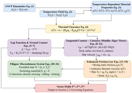
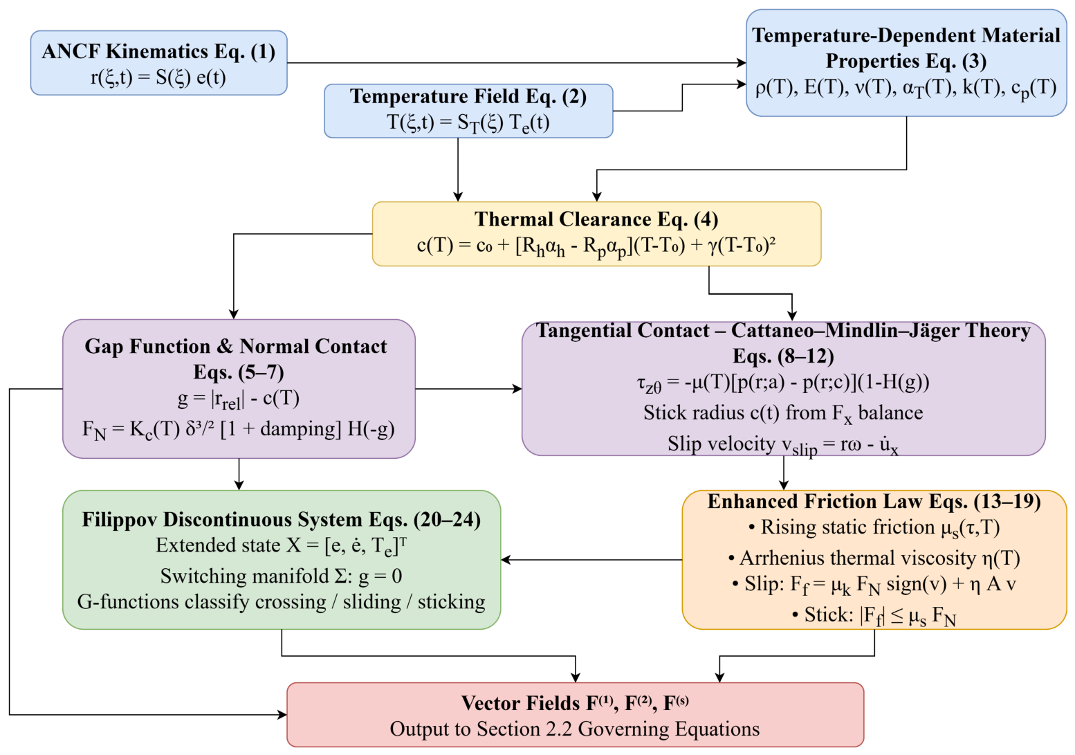
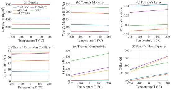
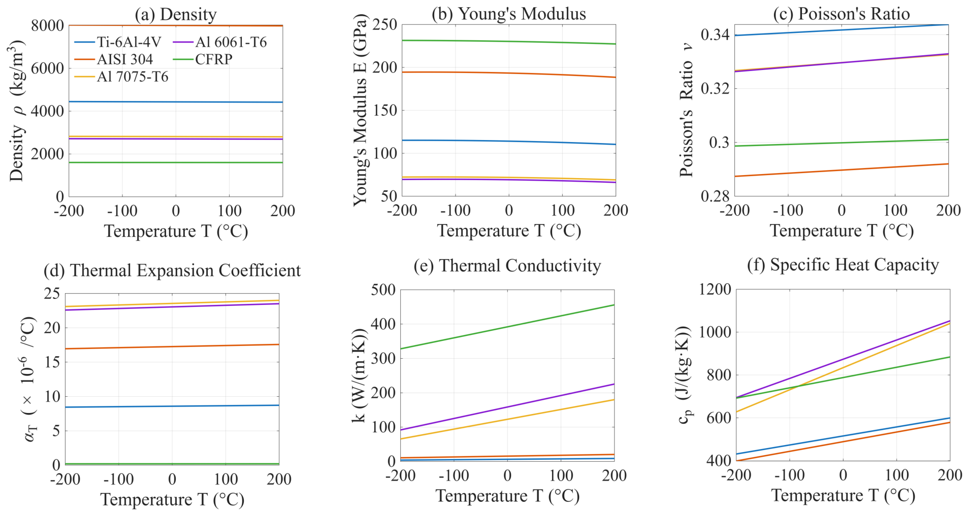
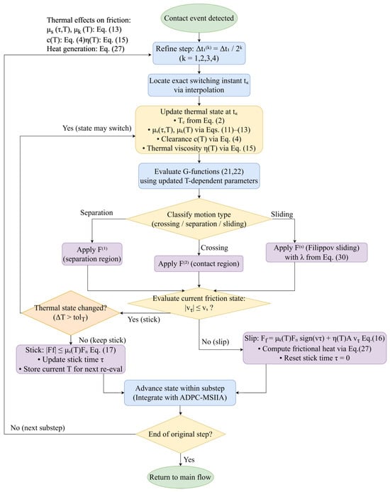
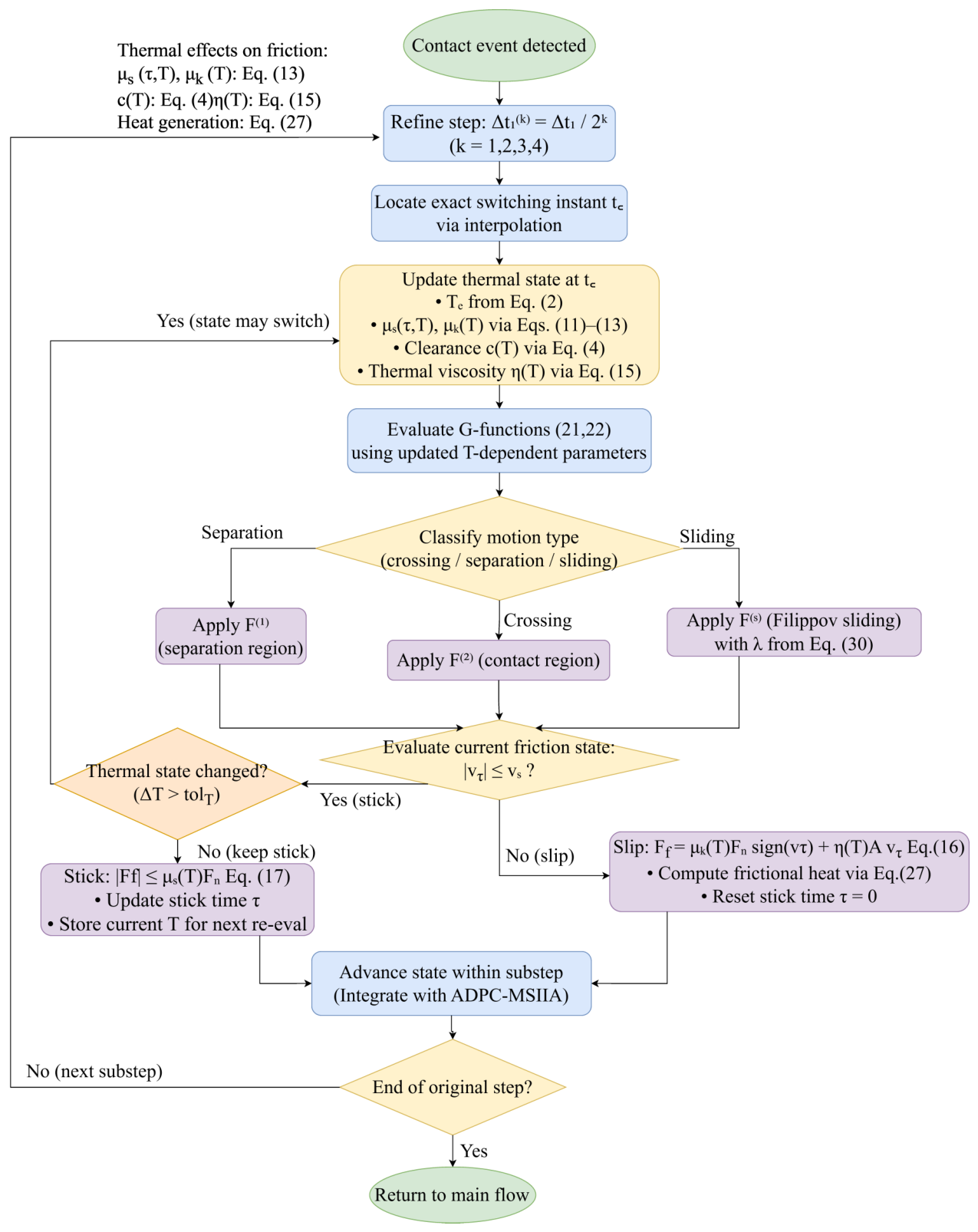
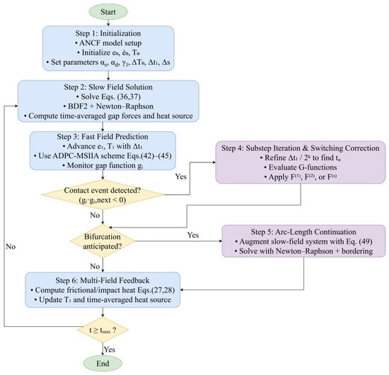
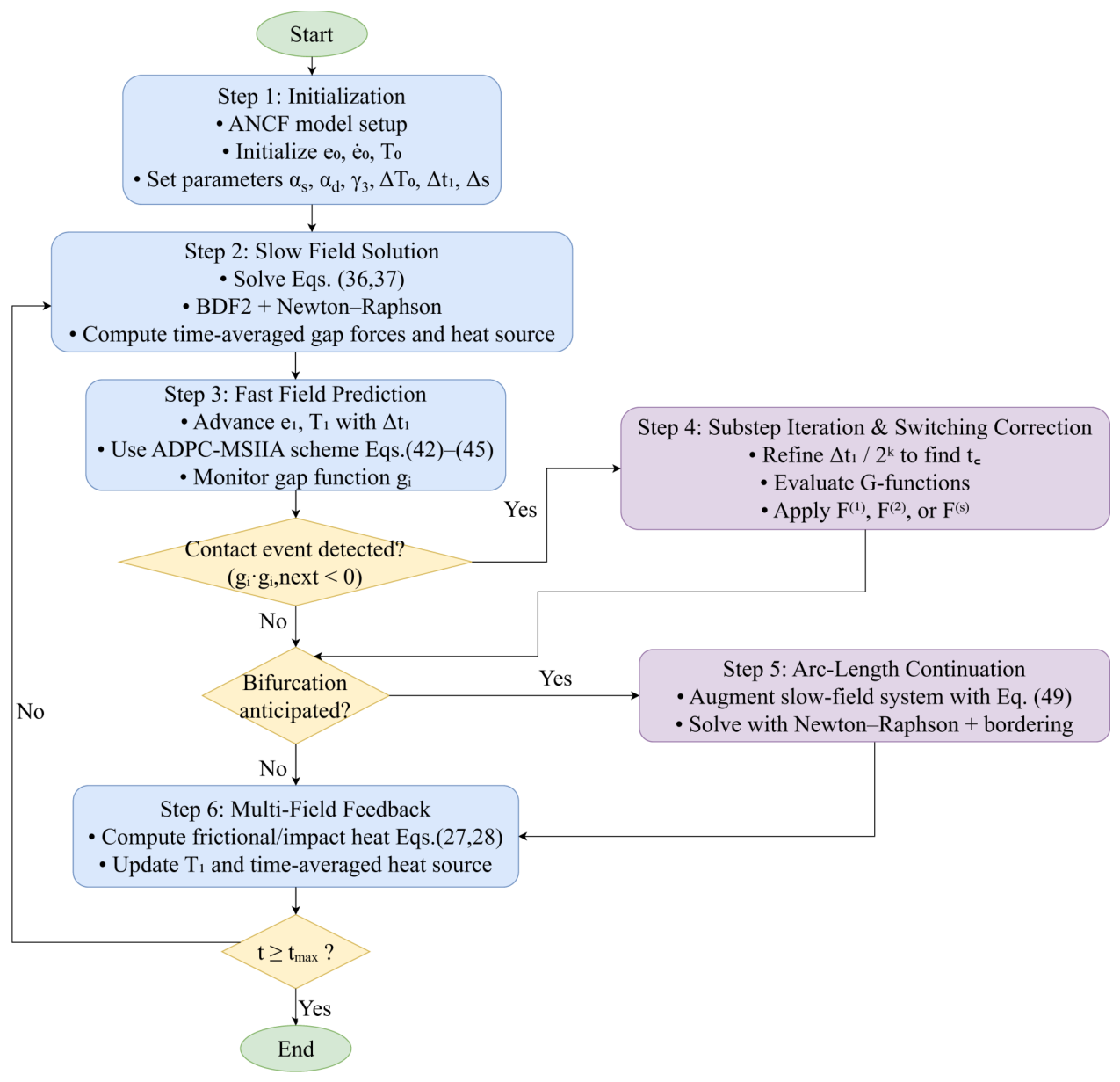
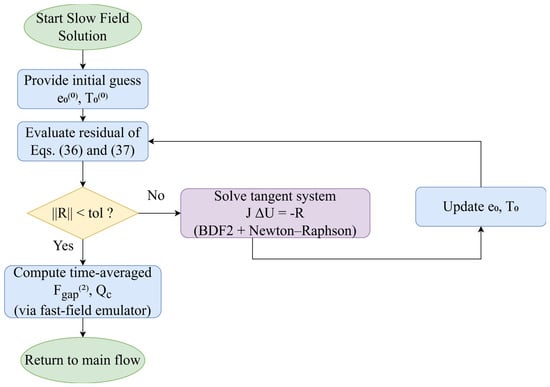
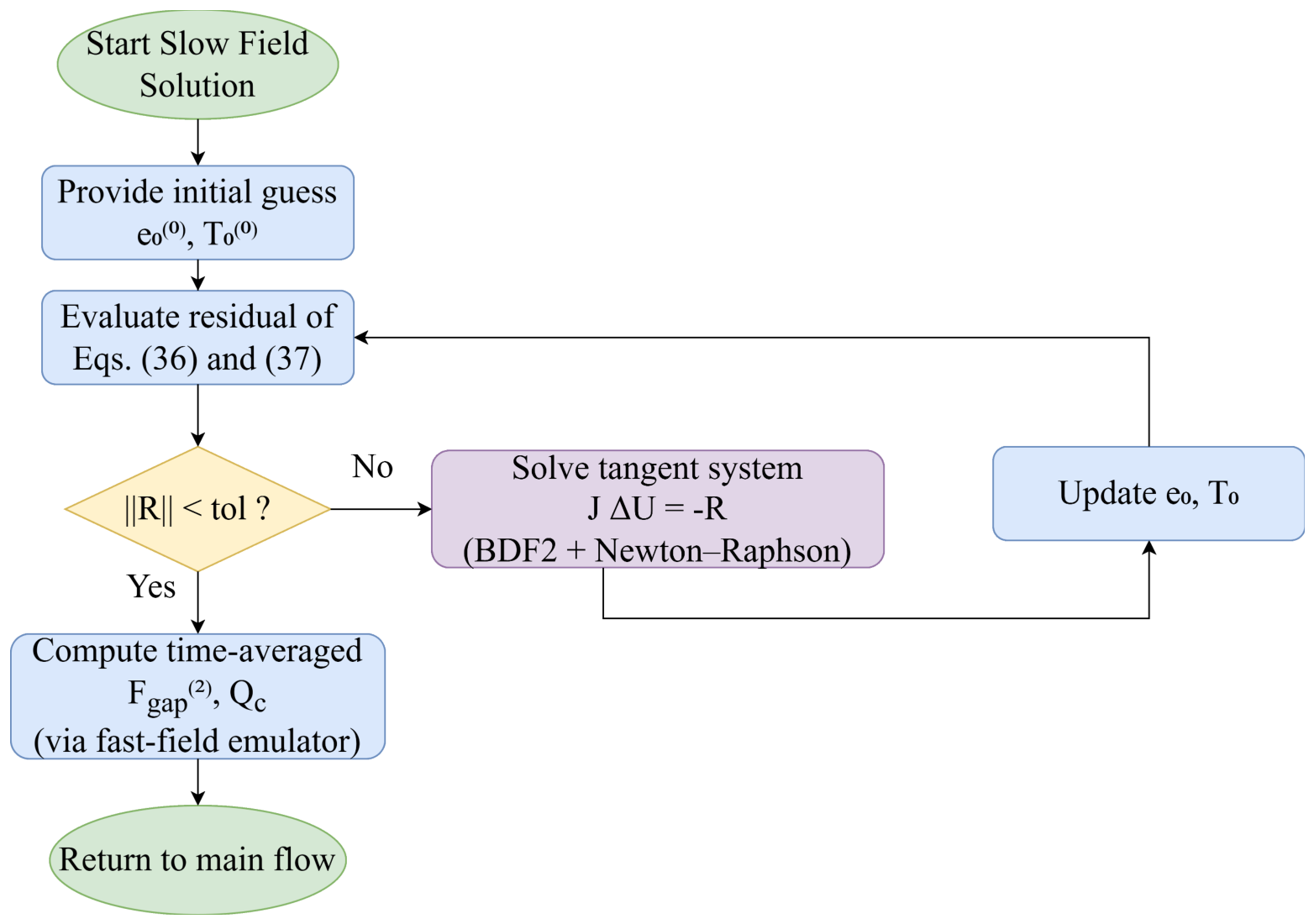
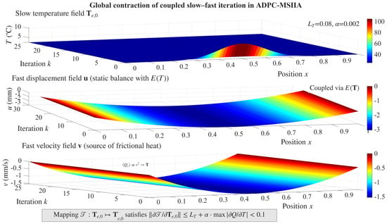
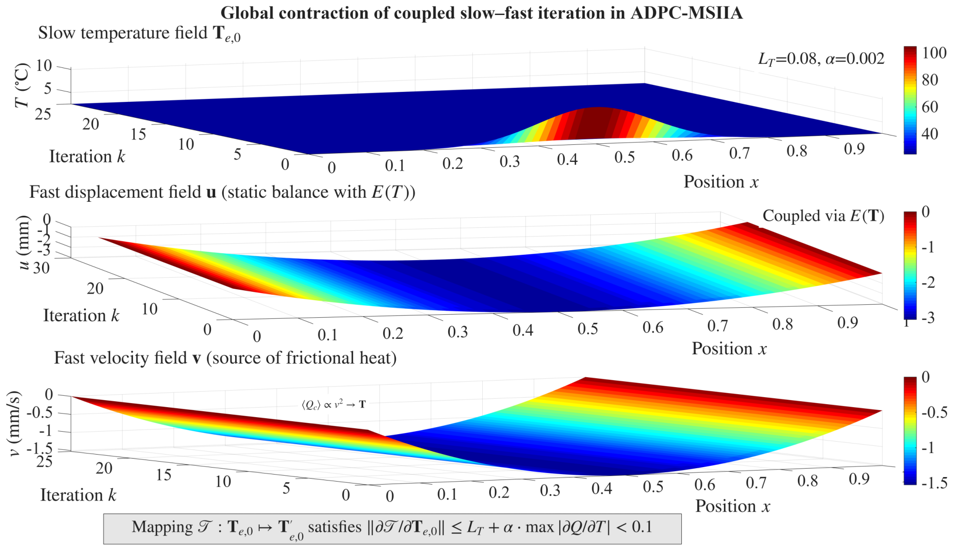
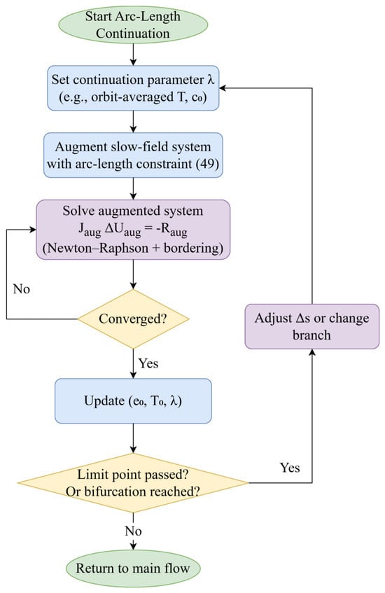
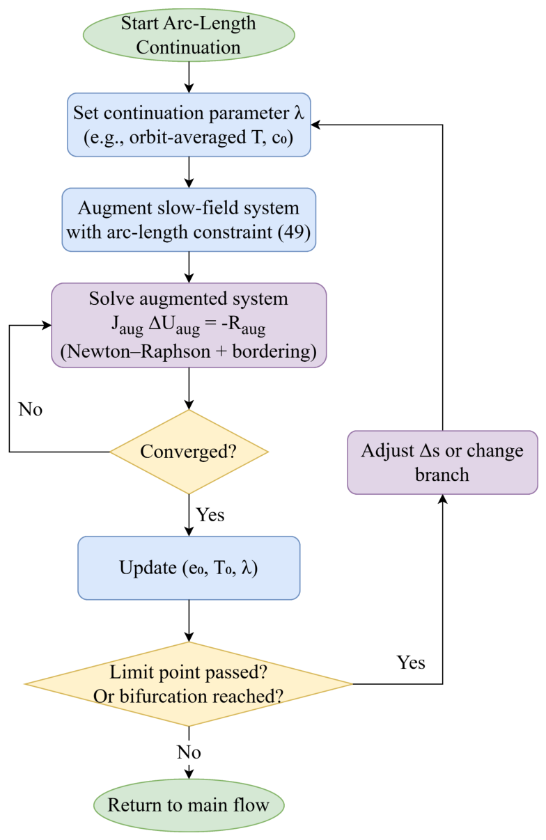
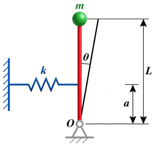
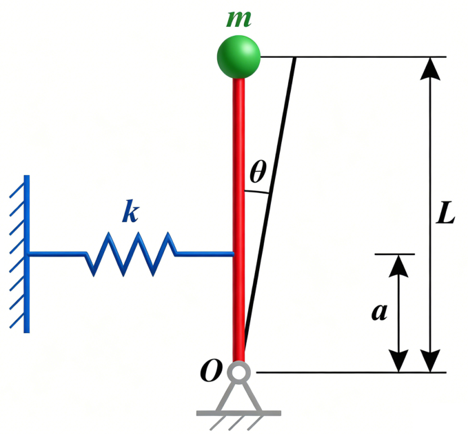
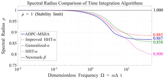
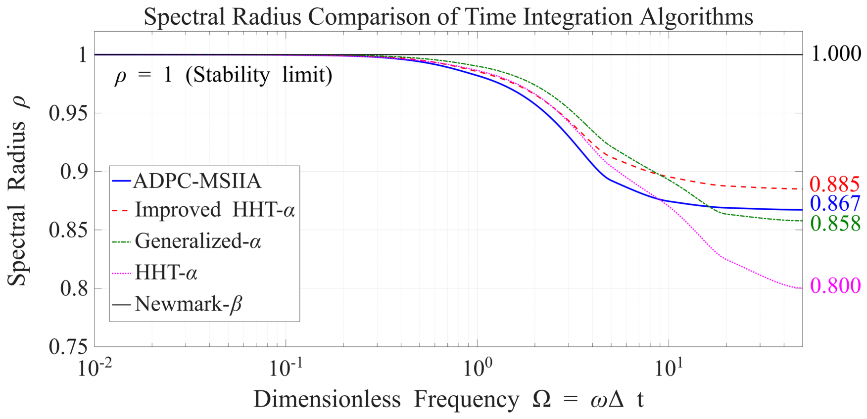
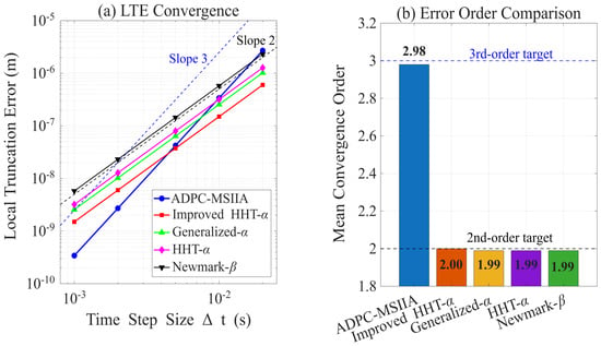
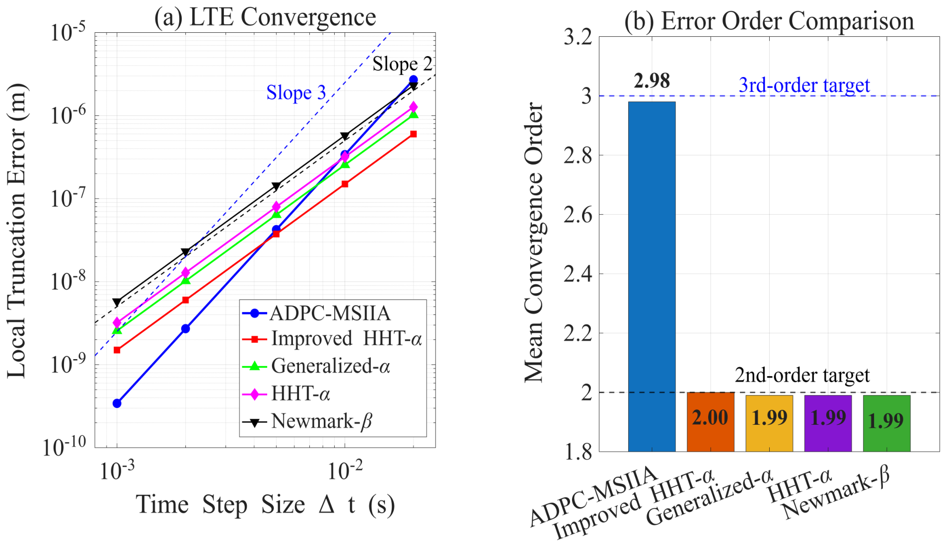
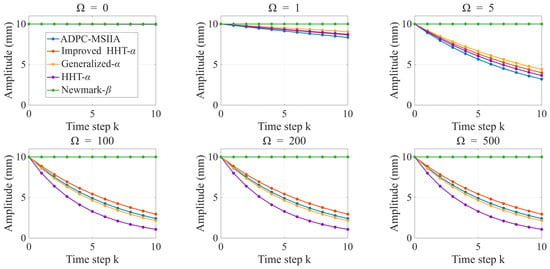
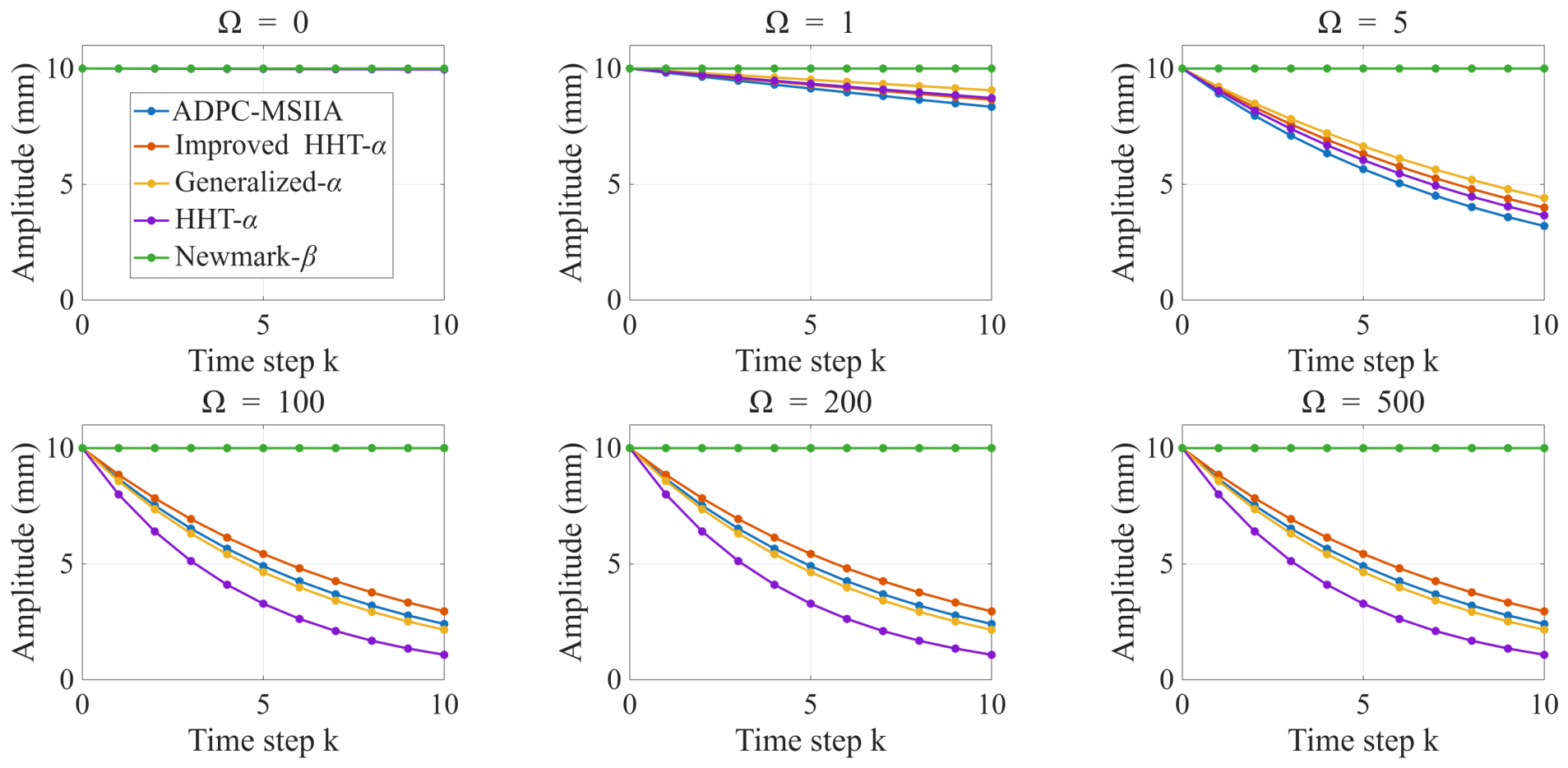
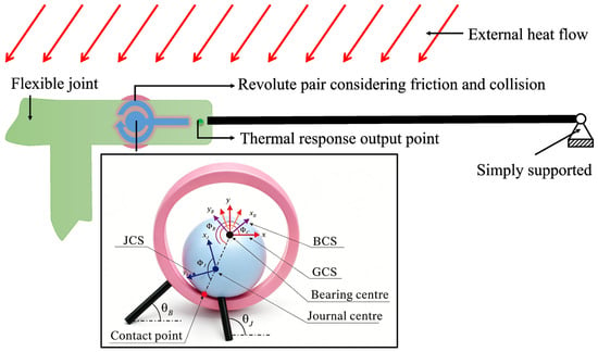
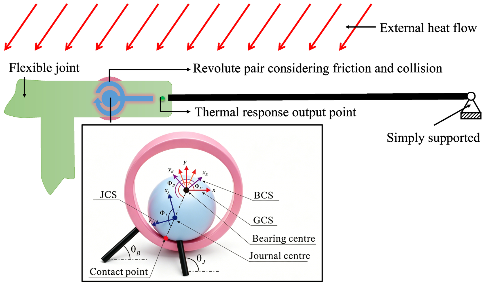
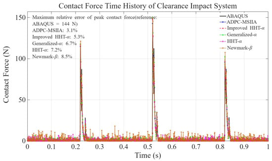
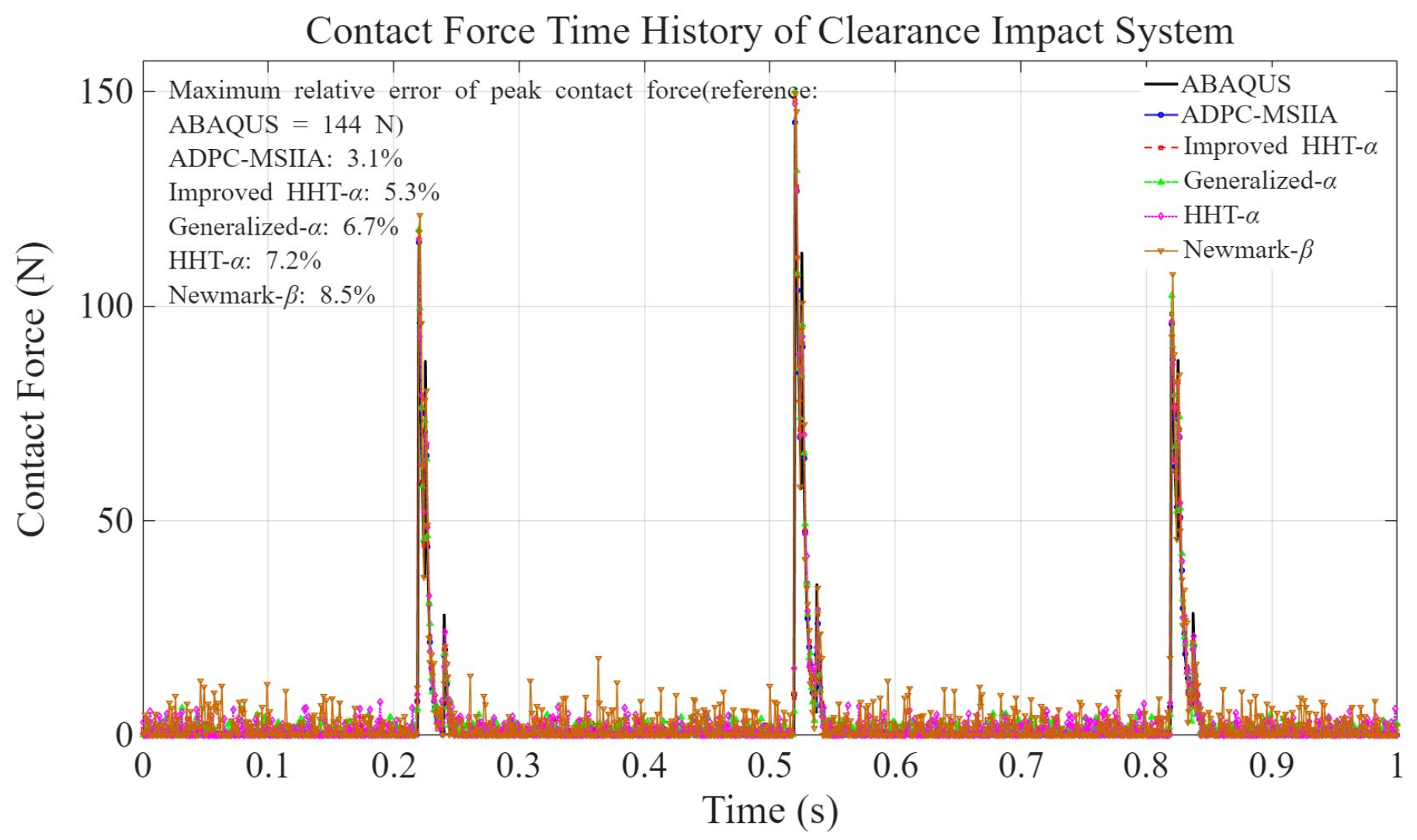
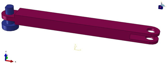
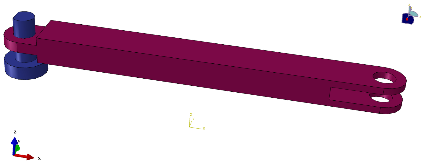
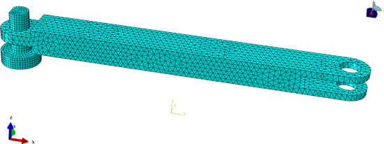
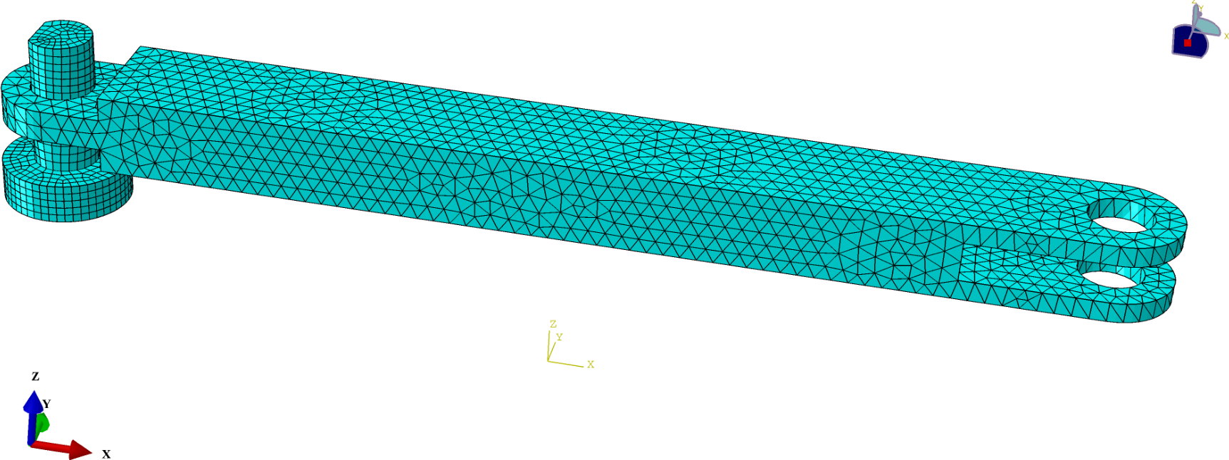
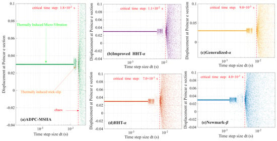
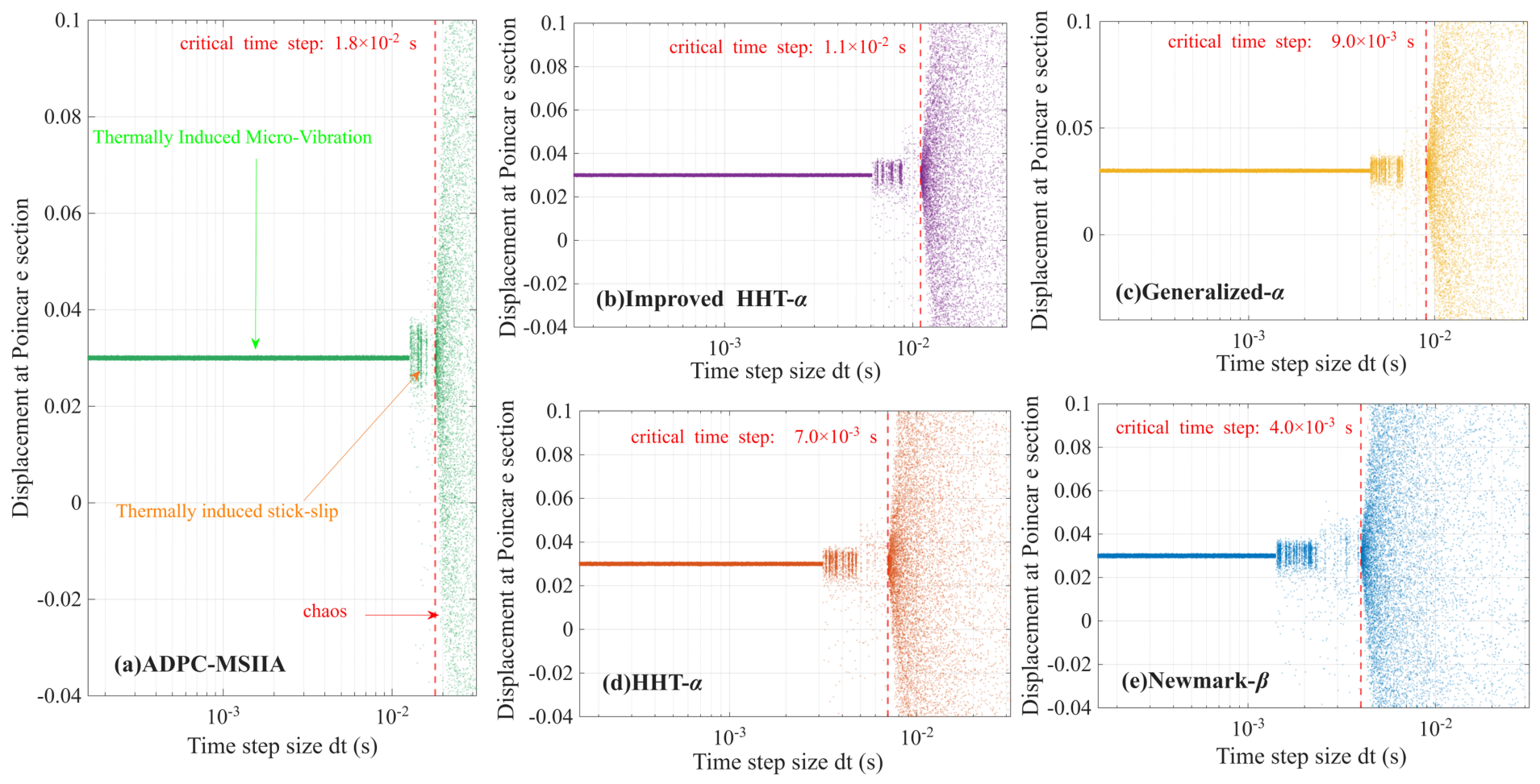
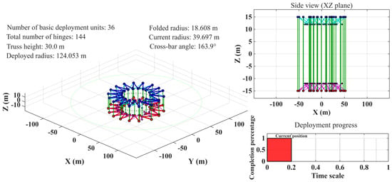
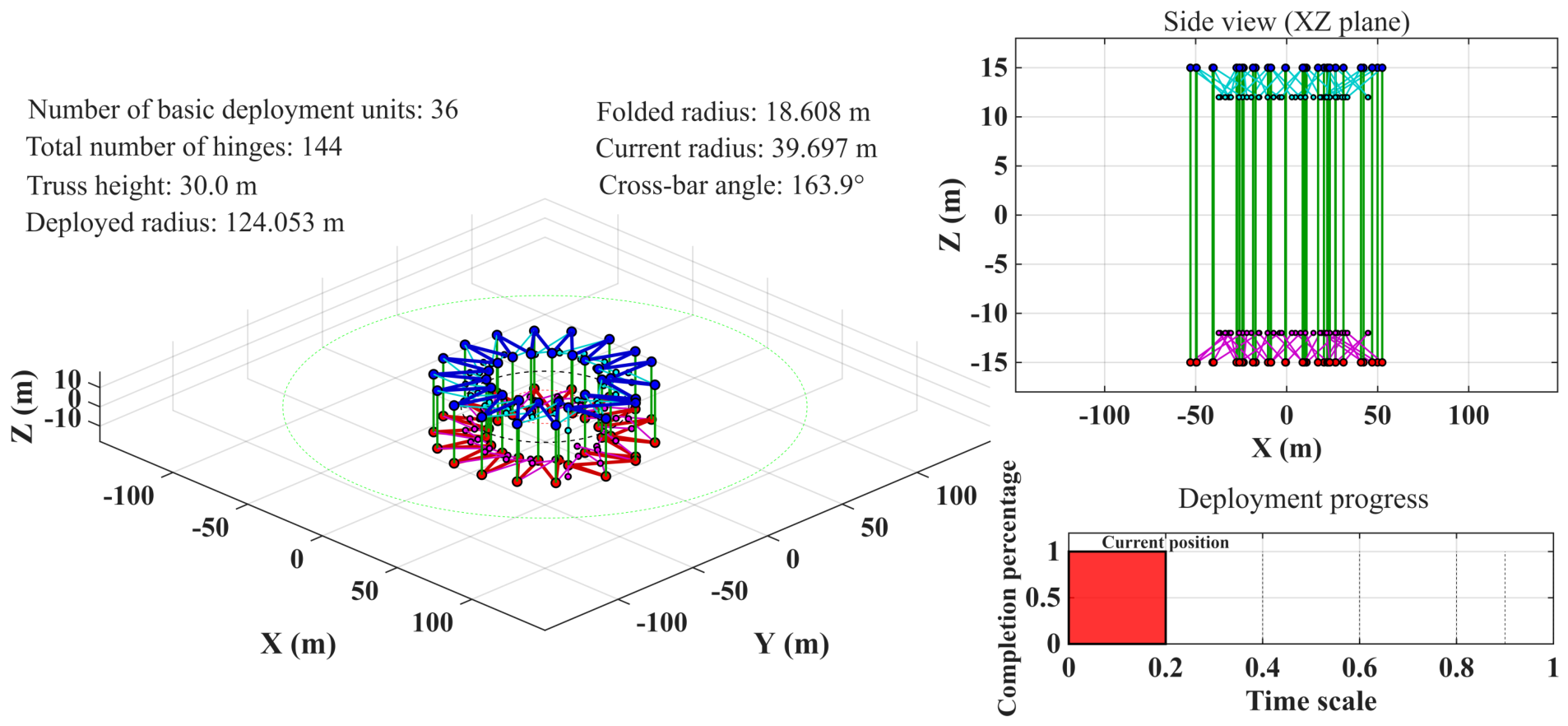
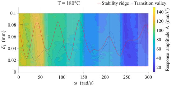
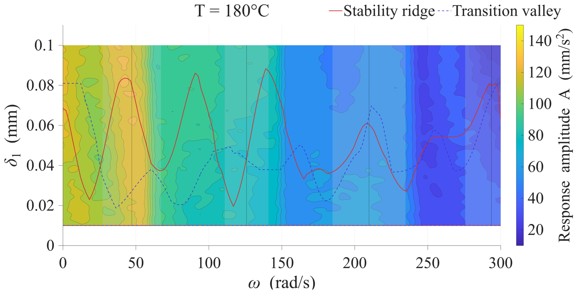
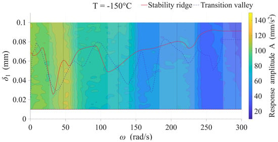
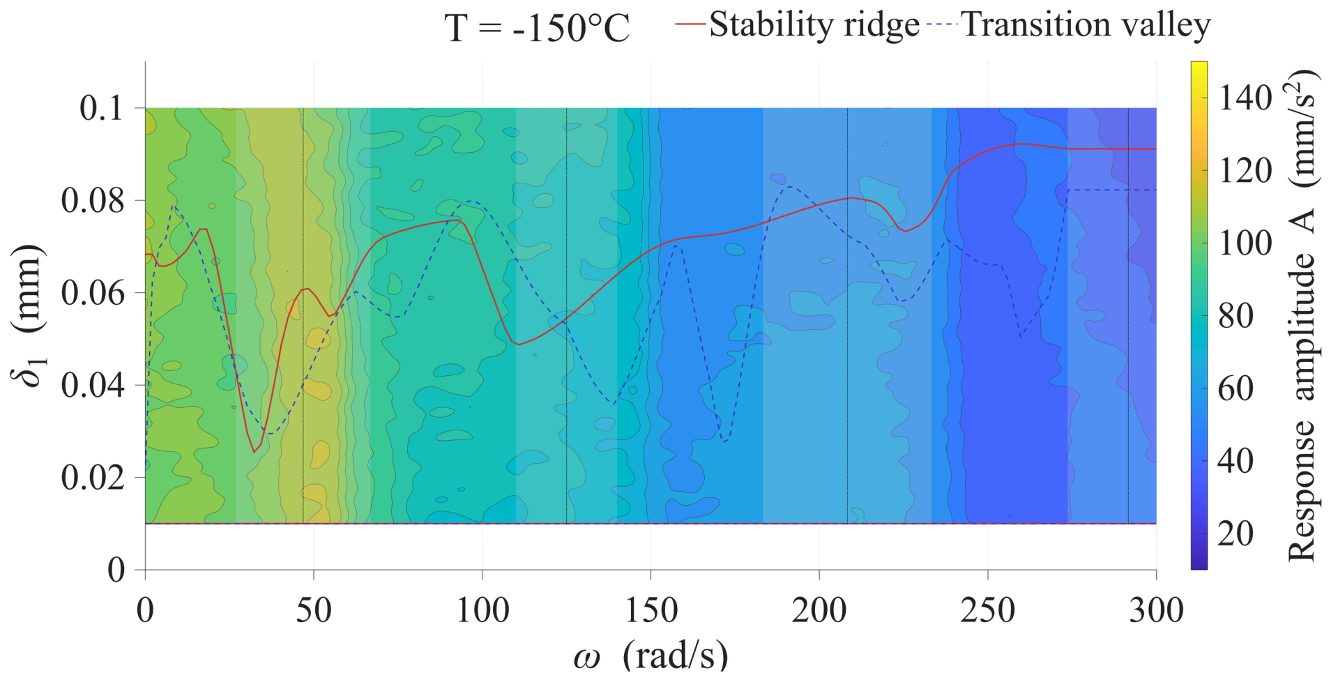
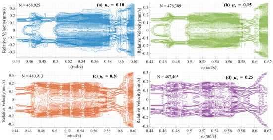
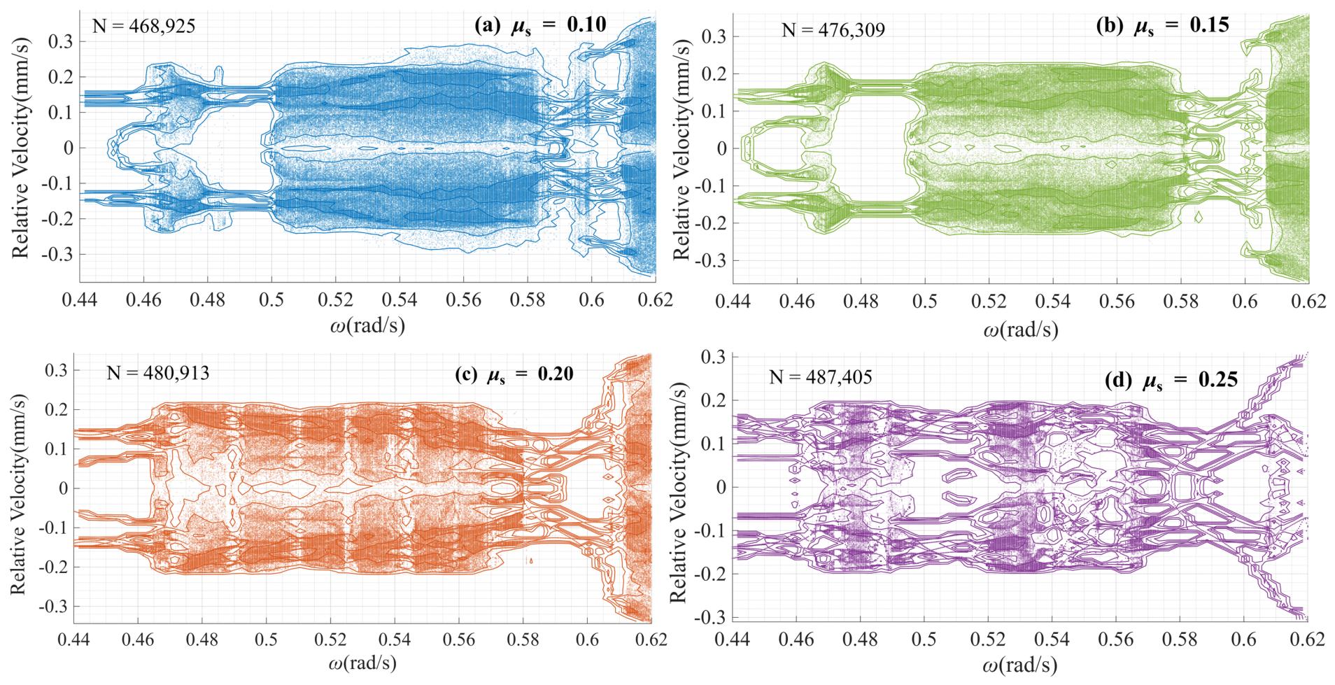
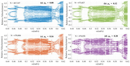
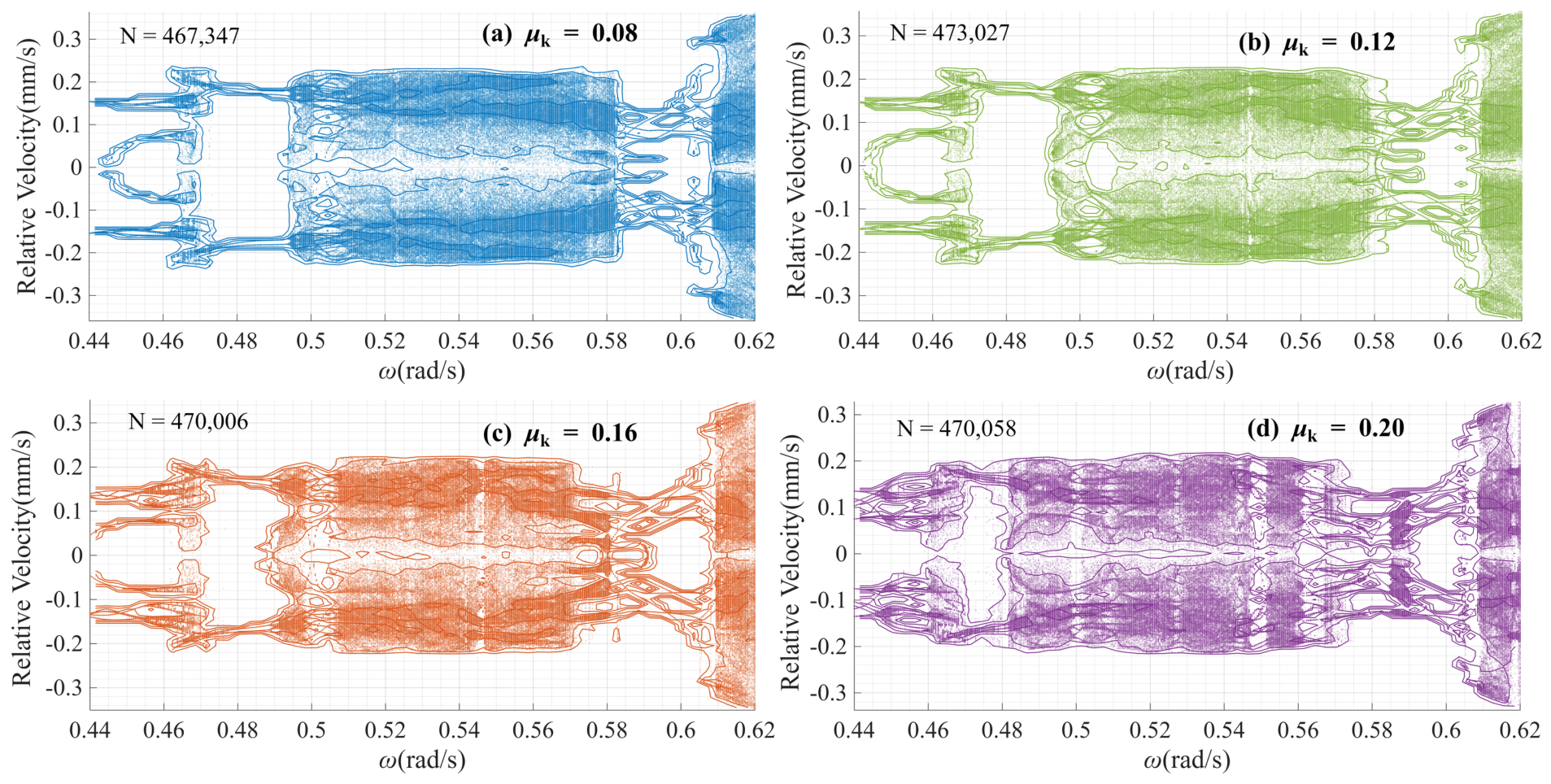
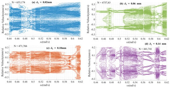
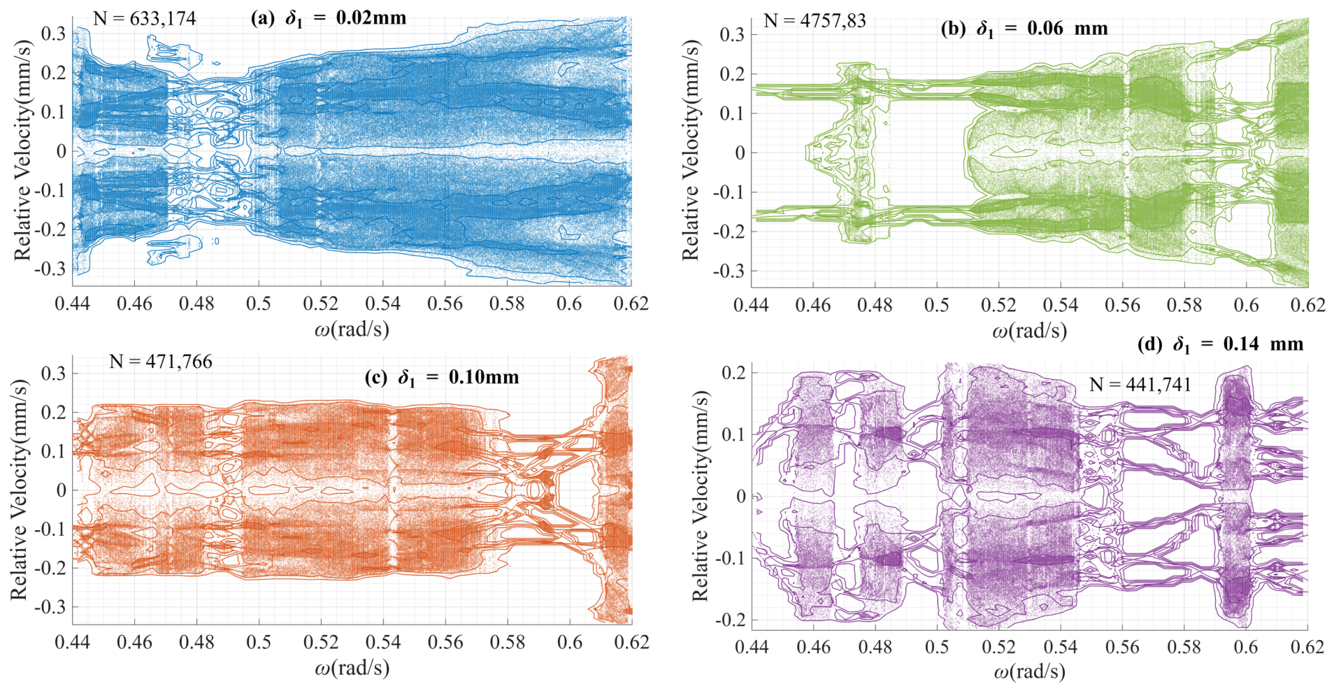
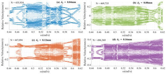
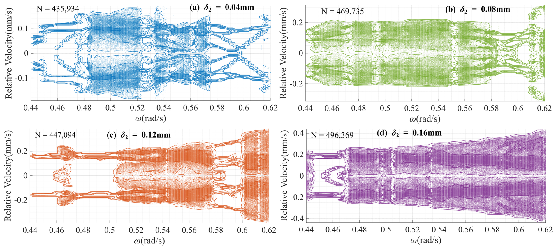
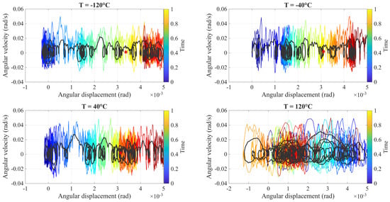
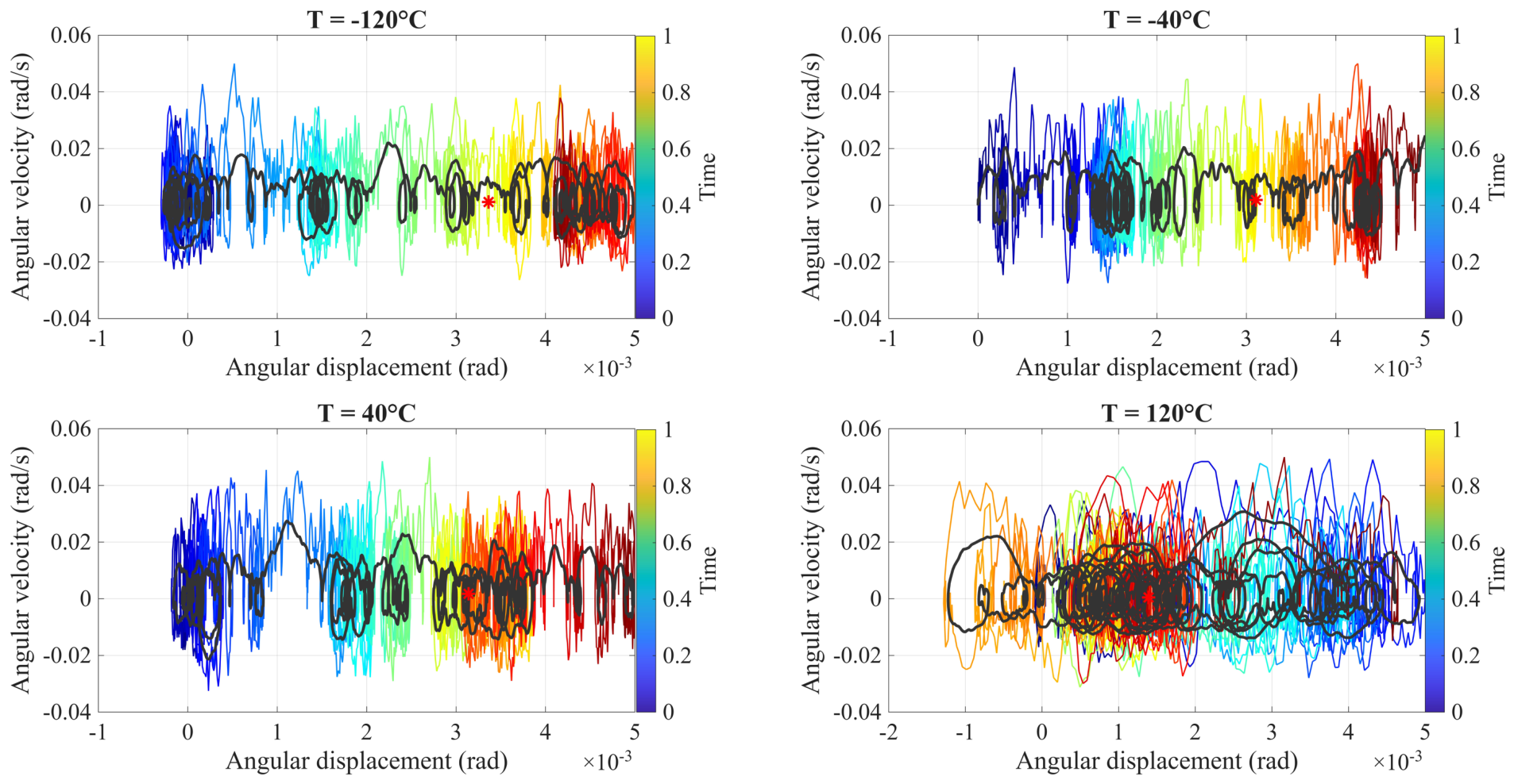
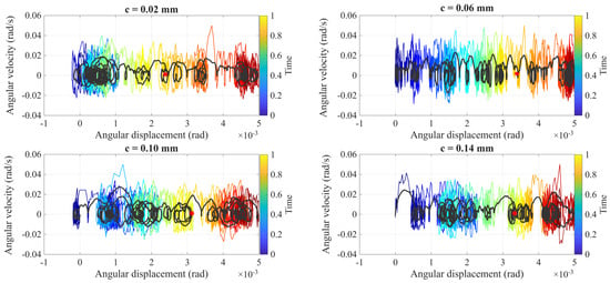
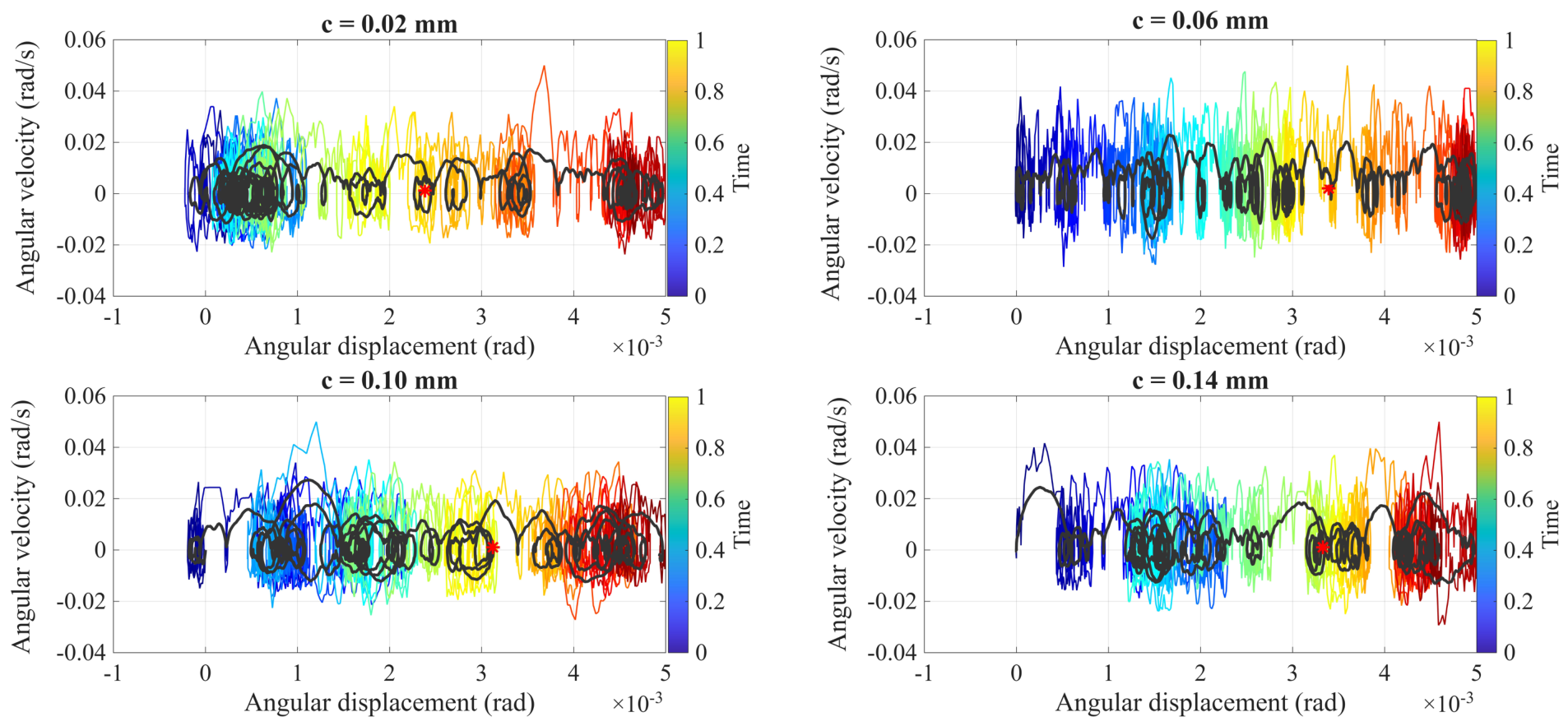

Disclaimer/Publisher’s Note: The statements, opinions and data contained in all publications are solely those of the individual author(s) and contributor(s) and not of MDPI and/or the editor(s). MDPI and/or the editor(s) disclaim responsibility for any injury to people or property resulting from any ideas, methods, instructions or products referred to in the content. |
© 2026 by the authors. Licensee MDPI, Basel, Switzerland. This article is an open access article distributed under the terms and conditions of the Creative Commons Attribution (CC BY) license.