


Abstract
This study aims to accurately estimate vertical tire forces on racing tires of specific stiffness using acceleration, pressure, and speed data measurements from a test rig. A hybrid model, termed Random Forest Assisted Deep Neural Network (RFADNN), is introduced, combining a novel deep learning framework with the Random Forest Algorithm to enhance estimation accuracy. By leveraging the Temporal Convolutional Network (TCN), Minimal Gated Unit (MGU), Long Short-Term Memory (LSTM), and Attention mechanisms, the deep learning framework excels in extracting complex features, which the Random Forest Model subsequently analyzes to improve the accuracy of estimating vertical tire forces. Validated with test data, this approach outperforms standard models, achieving an MAE of 0.773 kgf, demonstrating the advantage of the RFADNN method in required vertical force estimation tasks for race tires. This comparison emphasizes the significant benefits of incorporating advanced deep learning with traditional machine learning to provide a comprehensive and interpretable solution for complex estimation challenges in automotive engineering.
1. Introduction
The estimation of vertical tire forces exerted on racing tires is an important cornerstone in vehicle dynamics and motorsport engineering. This aspect is fundamental, as the enhanced grip significantly influences a racing vehicle’s speed, safety, and cornering abilities, which are essential under the high-speed and often variable conditions encountered in competitive racing.
Real-time monitoring of vertical tire forces is fundamental for ensuring driving safety and handling stability. Several studies propose algorithms to combine intelligent tire technology with neural network theory to estimate vertical forces effectively, such as Gu et al. [1]. The importance of accurately predicting vertical forces for advanced vehicle control systems is a popular technology.
Engineers tailor suspension configurations by accurately assessing vertical loads that offer the optimum balance between responsiveness and stability. This balance is crucial to maintaining high speeds while driving on the complex dynamics of a racetrack. The research by Ding et al. [2] underscores the importance of accurately estimating vertical forces as part of a broader vehicle stability framework. Furthermore, Li et al. [3] explore various vertical load estimation methods. Their findings reveal that accurate vertical load estimation is critical for optimizing tire utilization and enhancing vehicle handling and stability.
According to the internal reports of the Cyber Tire Team of Pirelli Factory, who are the official tire manufacturer for the Formula 1 competition, analyzing vertical forces that act on racing tires allows for teams to better understand and predict tire wear and suspension component durability, aiding in strategic decisions about pit stops and car setups, and ensuring that the vehicle maintains peak performance throughout the race.
The road-holding and braking performance of road vehicles is largely determined by the forces and moments acting on them. Accurately measuring or estimating these tire forces and moments is crucial for analyzing and controlling vehicle behavior [4]. Typically, traditional vehicle control systems estimate vertical tire forces using observer- based methods based on data from onboard sensors. However, these methods often rely on simplified vehicle models to estimate tire-related variables, especially in longitudinal and lateral dynamics. This reliance can lead to unreliable estimates under challenging conditions, such as sudden wheel load fluctuations, and can cause significant uncertainties primarily due to the use of these simplified models. Secondly, certain parameters within these tire models vary as the tire wears, leading to inaccuracies in the tire model. This requires periodic calibration of tire characteristic tests [1].
Despite the importance of vertical force estimation, there are significant problems in the literature. In the literature, parameters that are irrelevant, excessive, or insufficient in relation to those directly affecting vertical force have often been used. This has negatively impacted the accuracy of analyses. Most studies have relied on measurements taken from outside the tire. However, this approach has allowed for external vehicle data to interfere, leading to distorted estimations. Additionally, the datasets commonly used in the literature often fail to include the correct parameters, and the absence of sensors capable of measuring from within the tire has further hindered the ability to achieve accurate results.
In this study, acceleration, speed, and internal pressure were used to achieve better MAE values, which directly affect the vertical force. This study focuses on the parameters that directly affect the vertical force and aimed to address a significant gap in the literature by avoiding common problems such as using the wrong parameters. In this study, a novel hybrid approach called Random Forest-Assisted Deep Neural Network (RFADNN) is proposed to estimate vertical force, and this approach combines the strengths of other models. This approach integrates the feature extraction capability of deep learning methods with the nonlinear relationship processing capability of the Random Forest Algorithm.
The proposed hybrid method uses a mixture of various neural network layers to extract complex features from raw data. These features are then fed into a Random Forest model for tire force estimation. The necessary training and test data were obtained using a test rig equipped with a ‘drive-hard’ (DHF) racing tire rated as Shore A hardness 71 according to ASTM D2240 measurement standards in the established experimental environment.
The contributions of the proposed study to the literature are as follows:
- A novel combination of the strengths of deep neural networks and Random Forests has been used to estimate vertical tire forces better than existing related studies.
- A highly reliable dataset of racing tires with a specific hardness level has been obtained. The tests were performed using an original test rig setup in a racing tire manufacturer’s factory to simulate the original behavior of the racing tire.
- One of the important contributions is the use of inputs directly related to the vertical force for more realistic estimation. Acceleration, speed, and tire internal pressure values were used instead of irrelevant values used in the literature.
- The labeling of analog data representing the acceleration acting on the tire was automated using deep learning to reduce labeling effort and enhance reliability.
The rest of the paper is organized as follows: Section 2 reviews related works. Section 3 outlines the design steps of the proposed method. Section 4 introduces the data acquisition setup, data preprocessing stage, corresponding datasets, and data labeling. In Section 5, performance metrics are exclusively used to compare the proposed estimation method with others, and the comparative results are presented in a table. Additionally, estimation graphs illustrating the method’s performance are included. Finally, Section 6 offers concluding remarks.
2. Related Works
The realm of tire force estimation in vehicle dynamics is a well-explored area characterized by a rich history of evolving methodologies and technologies. This section delves into the significant body of related work, providing context and background to the advancements made in this field. The literature review is split into two distinct subsections to offer a comprehensive overview. The first subsection focuses on traditional estimation and estimation studies, specifically those utilizing observer and filter-based methods. These methods have laid the groundwork for understanding and predicting vertical tire force. The second subsection shifts attention to recent developments, exploring studies employing neural networks and deep learning-based approaches. These innovative methods represent a paradigm shift in tire force estimation, leveraging the power of machine learning and data-driven analysis.
2.1. Observer and Filter-Based Estimation of Vertical Force
This subsection focuses on previous notable contributions in the field of observer and filter-based estimation techniques, particularly in the context of vertical tire force estimation.
The research of [5] employs estimation modules to calculate/estimate tire forces using nonlinear observers. These observers utilize measured longitudinal acceleration, measured lateral acceleration, and measured vertical acceleration to estimate the vertical force. Additionally, an observer block is developed to compute the vertical tire forces based on the acceleration of the vehicle’s sprung mass in longitudinal, lateral, and vertical directions, as well as rotation around the roll and pitch axes.In this study, the vertical force estimation model relies on several vehicle geometric parameters, including the height of the center of gravity (), the height of the roll center (), the longitudinal distances to the front and rear axles (, ), and the front and rear axle widths (, ). The model assumes constant vehicle mass and a fixed center of gravity height (), which may not reflect dynamic loading conditions or changes in weight distribution. Its accuracy depends on precise measurements or estimates of these parameters, as any deviation directly affects the force distribution calculations. The model requires roll () and pitch () angle estimations, which rely on additional sensor data and filtering processes.
The study of [6] establishes an intelligent tire prototype based on microelectromechanical system accelerometers. The research proposes a theoretical rolling kinematics model to elucidate the mechanisms of acceleration fields resulting from the coupling effect of rigid body motion and elastic deformation. Additionally, the study formulates an analytical model for real-time estimation of vertical force.The vertical force is formulated as a function of the contact patch length and fitting coefficients, where the contact patch length is estimated using radial acceleration data. The model’s fitting coefficients are derived from experimental data under specific conditions, necessitating recalibration for different scenarios.
In the study by [2], the longitudinal, lateral, and vertical tire forces are individually estimated utilizing a strong tracking unscented Kalman filter and a conventional Kalman filter. These estimations utilize input parameters including yaw acceleration and lateral and longitudinal forces, while the filters make use of vehicle dynamic models.The vertical force estimation model relies on roll dynamics, requiring parameters such as roll angle () and roll acceleration (), which make the model dependent on the accuracy of the roll dynamic model. Suspension dynamics, including spring compression () and compression rate (), are incorporated, necessitating precise measurements from suspension height sensors. The model involves nonlinear equations that depend on parameters such as spring stiffness () and damping coefficient (), which require accurate calibration. Additionally, the model assumes small roll angles () to apply linear approximations (, ), potentially limiting its accuracy under conditions involving larger roll angles. The effects of unsprung mass dynamics are not explicitly included, which may influence predictions in scenarios with significant dynamic load variations.
The research by [5] introduces a Tire Vertical Force Observer (TVFOB) to estimate the vertical forces acting on tires by using suspension deformation and acceleration data from both the sprung and unsprung masses. The method leverages a quarter-car model, which simplifies the suspension system dynamics for analysis and observer design. The state-space model incorporates suspension deformation, sprung mass acceleration, and tire deformation as states, assuming the derivative of tire deformation and road surface vertical position changes follow white Gaussian noise. The proposed observer relies on measurable quantities, such as suspension deformation (distance between sprung and unsprung masses) and sprung mass acceleration.
The authors of [7] design an estimation system for vertical tire forces in a four-axle truck used for vehicle dynamic control based on an adaptive treble-extend Kalman filter.The vertical force estimation method relies on a four-axle truck model, which introduces challenges due to the over-constrained nature of the system and the variability in center of gravity positions caused by uneven load distributions. The method also depends on roll dynamics, requiring accurate measurements of roll angle, roll acceleration, and rotational inertia, which can vary significantly in heavy vehicles with irregular load placements. Additionally, the model involves complex parameterization, including suspension stiffness, damping coefficients, and rotational inertia, necessitating precise calibration and updates for different operating conditions. While the approach aims to minimize sensor usage, it still relies on critical sensor data, such as roll rate measurements, which are essential for accurate dynamic updates and can impact the overall reliability of the model.
Wilson et al. in [8] present a parameterization procedure for tire vertical stiffness, focusing on measured tire geometry and air pressure, particularly for applications where high-fidelity tire models are deemed unnecessary. Vertical forces are computed through an air volume optimization approach. They compare this approach, known as the “Energy method”, developed by Harth et al. introduced in [9], for force estimation based on tire shape, with a proposed contact area-based approach (Area method) and an approach by Rotta (Rotta method). These methods are employed for estimating vertical forces acting on a tire on flat ground with various deflections, with the Energy method outperforming the others.The vertical force estimation method in the paper relies heavily on the geometric properties of the tire, including free radius, sidewall length, and rim diameter. The method requires accurate measurements of these parameters to calculate the contact patch length, which directly influences the predicted vertical force. The reliance on specific tire geometries and contact patch characteristics makes the model sensitive to parameter variations and limits its generalizability to other tire types or dynamic scenarios. Moreover, the use of fitting coefficients derived from experimental data introduces a dependency on specific conditions, necessitating recalibration for diverse applications. The sensitivity of the model to parameter variations is demonstrated in the tables within the paper, where a 5% change in parameters, such as free radius or sidewall length, results in significant deviations in force estimation. This highlights the importance of precise geometric measurements and calibration. Additionally, the requirement for sensor data, such as radial acceleration, adds complexity to the implementation, as sensor noise and environmental factors may further affect prediction accuracy. These limitations underscore the method’s reliance on accurate parameterization and robust calibration.
The authors of [10] propose an estimator based on an unscented Kalman filter (UKF) for estimating the roll angle and lateral acceleration using the UKF algorithm for a Three-Degree-of-Freedom (3-DOF) model. Subsequently, the research employs lateral load transfer and longitudinal load transfer models to estimate the vertical load force on each tire.The proposed vertical force estimation method relies on a 3-DOF vehicle model and a lateral–longitudinal load transfer model, both of which require a range of dynamic parameters. The 3-DOF model incorporates roll dynamics and necessitates precise measurements of roll angle (), roll rate (), and lateral forces (), as well as suspension stiffness and damping coefficients. Similarly, the lateral–longitudinal load transfer model depends on parameters such as wheel radius (R), vehicle width (B), and the height of the center of gravity (H), alongside lateral acceleration (). While these models enhance the method’s ability to capture dynamic effects, their reliance on detailed parameterization and accurate sensor measurements increases complexity.
The study by [11] proposes an algorithm to estimate the dynamic components of vertical tire contact forces by measuring vehicle body acceleration and angular velocity at selected locations on a standard vehicle. This involves employing a Kalman filter with augmented tire forces in the system state vector.The vertical force estimation method employs simplified vehicle models, such as the half-car model, which are computationally efficient, but do not fully capture complex real-world dynamics, including suspension system interactions and detailed tire-road behavior. The method shows error rates under varying road roughness and vehicle speed conditions, which can limit its applicability across diverse scenarios. The use of body-mounted sensors restricts the precision of tire force estimation, as alternative sensing technologies, such as tire-mounted sensors, are not included. Additionally, the method adopts a random walk model for tire force evolution, which simplifies the estimation process, but does not incorporate physical relationships between time steps. The computational feasibility and real-time performance of the approach are not discussed in the study. Finally, the robustness of the Kalman filter to sensor noise and modeling errors is constrained by the method’s design, potentially affecting its performance in practical applications.
The research by [12] introduces new vehicle dynamics models for estimating vertical, longitudinal, and lateral tire forces. Nonlinear observers are utilized to predict tire forces.The proposed vehicle model for vertical force estimation captures suspension pitch and roll dynamics, offering a novel approach to link suspension motion with tire forces. However, it has certain limitations. The model simplifies real-world vehicle dynamics, which may reduce accuracy during extreme maneuvers or on highly variable road surfaces. Its reliance on ADAS map data, such as road slope and friction coefficients, makes it susceptible to inaccuracies or outdated information in these maps. Additionally, the model’s performance is sensitive to sensor noise and requires precise parameter tuning, as small inaccuracies in input data or parameter settings can significantly affect the estimated forces.
The authors of [13] put forward a method for estimating individual tire vertical forces using a steady-state weight transfer approach that takes into consideration the roll stiffness distribution. In this approach, unsprung masses and suspension dynamics are disregarded, and the front and rear roll center heights are assumed to be at ground level. Additionally, the road is assumed to be completely flat, and dynamic loads resulting from road irregularities are not considered. Lateral weight transfer is presumed to be dependent on the roll stiffness at each axle.The proposed method aims to reduce tuning efforts by avoiding the complexities of traditional tire models and instead relies on a steady-state weight transfer approach combined with roll stiffness distribution for vertical force estimation. However, this simplification introduces certain limitations. The neglect of suspension dynamics and transient effects restricts the model’s accuracy under dynamic driving scenarios such as uneven road surfaces. Additionally, while the reliance on roll stiffness distribution reduces the need for extensive parameter tuning, inaccuracies in these parameters can still significantly impact the estimation performance.
In [14], the contact angle between the tire and the road surface is calculated using an intelligent tire and is subsequently employed for tire load estimation.The vertical force estimation method described in this study demonstrates certain limitations that could affect its effectiveness in real-world applications. The simplified vehicle model used does not account for factors like air resistance or road surface irregularities, which could restrict its applicability in more complex environments. While dynamic load estimation has been validated against a vehicle dynamics model, further verification using direct measurements with wheel force transducers would strengthen its reliability. Additionally, reliance on geometric assumptions may reduce its accuracy on inclined or uneven road surfaces.
Research by [15] proposes a method for estimating vertical load by deriving peak radial displacement from the radial acceleration signal. While effective within the tested conditions, this approach exhibits certain limitations. The integration process for the acceleration signal can introduce errors, including drift, which necessitates mitigation through high-pass filtering. Furthermore, the method assumes a linear relationship between peak radial displacement and load, but this assumption holds only within specific pressure and load ranges, potentially restricting its applicability to broader or more variable operating conditions.
M. Doumiatia et al. [16] propose an innovative observer for estimating one-sided lateral load transfer employing a linear Kalman filter. The estimated lateral load transfer, along with longitudinal acceleration measurements, is utilized for estimating vertical forces.The vertical force estimation method utilizes suspension deflection measurements to calculate the roll angle, which serves as a key component in determining the tire load distribution. While effective in controlled scenarios, the method presents some practical challenges. Suspension deflection measurements require precise sensors on each wheel, which can increase the complexity and cost of the system. Additionally, the accuracy of the estimations may be affected by sensor calibration issues or drift over time. The approach assumes linear roll dynamics and a fixed roll center position, which might not fully capture the complexities of real-world conditions, such as high-speed maneuvers or uneven road surfaces. Furthermore, factors like road surface variations, tire wear, and temperature changes are not explicitly accounted for, which could impact the model’s performance in diverse environments.
In [17], an empirical model is developed and comprises a basic shape function for acceleration and relationships that connect the parameters of this function to tire conditions. Furthermore, a model-based estimator is designed for vertical force using this model, which consists of a peak synchronization algorithm and an extended Kalman filter.
An increase in the complexity of vehicle or tire models does not necessarily translate to proportional improvements in prediction accuracy, and there are certain errors and uncertainties in the prediction of the tire force based on the signals collected by on-board sensors [1]. While increasing model complexity aims to capture the intricate dynamics of tire forces, it also introduces significant challenges in terms of parameter tunability and practical implementation. Complex models require highly accurate parameter estimation, which is often impractical due to variations in vehicle dynamics, road conditions, and tire wear. Additionally, the reliance on a larger number of sensors to improve model accuracy further escalates system costs and increases the likelihood of sensor malfunctions or failures.
These limitations highlight the inherent trade-offs in traditional model-based approaches, where greater complexity does not necessarily lead to better performance, but instead adds layers of calibration difficulties and operational risks. In this context, data-driven methodologies, supported by deep neural networks, enable the extraction of complex features from raw acceleration data, overcoming the limitations of traditional parametric models and enhancing prediction accuracy. By embedding accelerometers directly into the tire structure, high-fidelity data can be collected without the need for extensive external sensor arrays. This not only reduces system complexity, but also minimizes maintenance costs and failure risks associated with multiple sensors.
2.2. Hybrid and Pure Neural Network Approaches in Vertical Tire Force Estimation
The studies in this category use the robustness and sensitivity of the extended Kalman filter (EKF) as well as the adaptability and learning capabilities of neural networks in handling nonlinear systems. By integrating these two approaches, the aim is to alleviate the limitations of each method and provide a more accurate and comprehensive solution for estimating tire forces. The reviewed literature ranges from early applications of EKF in tire force estimation to more recent developments involving neural network architectures. This section will focus on how these hybrid methods improve estimation accuracy and provide a detailed discussion of their role in advancing tire force estimation technologies.
Tianli Gu et al. [1] use the Genetic Algorithm to optimize a Backpropagation (BP) neural network to predict vertical tire forces. This method takes advantage of the robust global search capability of the Genetic Algorithm to address the tendency of the BP neural network to get stuck in local minima. The input parameters for their algorithm include inflation pressure, speed, longitudinal data, contact patch length, radial displacement peak, and wear amount.The calculation of radial displacement relies on double integration of acceleration signals obtained from a accelerometer embedded in the tire. While this approach effectively derives displacement from acceleration, it is inherently sensitive to noise and drift in the raw acceleration data, which can significantly impact the accuracy of the displacement estimation. Moreover, the double integration process amplifies low-frequency noise, necessitating the application of filtering techniques that may inadvertently remove critical signal components.
In [18], a comparative analysis is performed on neural networks using the Resilient Backpropagation (Rprop) algorithm, Recurrent Neural Networks (RNN), and Random Forests (RFs) [19]. The method relies on indirectly identifying the tire contact patch using acceleration signals, which introduces potential limitations in accuracy. Variations in tire types and hardness may impact the reliability of the contact patch estimation.
Ref. [20] propose a method to describe radial loads on tire-tired vehicles using a one-dimensional Convolutional Neural Network (1D CNN) and a Bidirectional Gated Recurrent Unit (BiGRU). However, the method relies on onboard sensors mounted on the vehicle body and axles to measure physical quantities such as vertical and angular acceleration. While these sensors provide valuable data for estimating vertical force, their placement on the vehicle rather than directly within the tire structure introduces limitations. Onboard sensors are susceptible to noise, vibrations, and interference from the vehicle chassis and suspension system, which can degrade the accuracy of the force estimation. The vertical acceleration of the vehicle body, the vertical acceleration of the axles, pitch angular acceleration, rolling angular acceleration, and rolling angular acceleration are used as input variables. Then, the vertical forces at each wheel are used as outputs.
Sung Jin Im et al. [21] conducted a study on the normal forces exerted by tires on automotive vehicles using an LSTM model. The input data for LSTM models include pitch ratio, vertical velocity of the sprung mass, acceleration, rolling acceleration, and pitch acceleration.The vertical force estimation method proposed in the study, which employs an LSTM model, has limitations related to its data-driven structure and training process. The model is trained using simulation data generated using CarSim, which may not fully represent the variability in operational environments. Robustness analysis, as conducted within the study, indicates that the model is sensitive to parametric uncertainties, such as changes in vehicle mass and tire stiffness, and to sensor noise. While the model maintains accuracy under moderate levels of Gaussian noise, its performance decreases with higher levels of data contamination. These findings suggest that the LSTM model’s performance is influenced by the quality and diversity of the training data and its ability to handle deviations from the training parameters.
Guiyang Wang et al. [22] estimate tire forces using a neural network. The study successfully reduces the computational complexity and storage requirements of the system by using an improved Levenberg-Marquardt (LM) learning algorithm and self-organizing neurons. They also increase the estimation accuracy by incorporating EKF and Moving Average (MA). Input parameters used to estimate vertical force include front wheel angle, yaw rate, longitudinal velocity, longitudinal acceleration, lateral acceleration, wheel angular velocity, and road adhesion coefficient.However, the reliance on onboard sensors, such as IMUs and wheel speed sensors, introduces limitations due to the indirect nature of the measurements. These sensors are affected by noise and vibrations from the vehicle chassis, which can reduce the accuracy of tire force estimation.
Marco Viehweger et al. [23] introduce observer-based models for estimating vertical force. These models encompass an extended Kalman filter (EKF) scheme employing a linear tire model with stochastically adapted cornering stiffness, an EKF scheme employing a neural network (NN)-based linear tire model, a tire model-less Suboptimal-Second Order Sliding Mode (S-SOSM) scheme, and a Kinematic Model (KM) scheme integrated within an EKF.The analyzed methods, as presented in the study, exhibit various limitations that affect their performance and applicability. The extended Kalman filter (EKF) with a linear tire model struggles with capturing tire–road interactions under nonlinear conditions and suffers from observability issues during low dynamic scenarios. The EKF with a neural network-based tire model is highly dependent on the quality and diversity of the training data, limiting its generalization to unseen conditions. The Suboptimal Second-Order Sliding Mode (S-SOSM) method relies heavily on accurate parameter estimation and requires significant tuning, particularly for the EKF stage, while its assumption of a flat road reduces its robustness under varying road inclinations. Lastly, the kinematic model integrated with EKF fails to account for dynamic effects, depends on precise IMU placement, and is sensitive to observability issues during straight-line motion, leading to reduced accuracy. These limitations, as demonstrated in the analyses conducted within the study, underscore the challenges in achieving robust and adaptable estimation techniques.
2.3. Analysis of Methodological Constraints in Related Works
2.3.1. Peak Radial Displacement-Based Approaches
In [2,15], peak radial displacement () is calculated as the radial displacement derived from the double integration of radial acceleration () over the contact patch traversal time (). The formula is expressed as follows:
where:
- : radial acceleration signal measured during tire–ground interactions;
- : the time required for the tire to traverse the contact patch, which serves as the integration limit.
The contact patch traversal time () is calculated as the time difference between the local extremum pointsin the radial acceleration signal, corresponding to the leading and trailing edges of the contact patch. However, the identification of these extremum points is sensitive to noise in the acceleration signal, which can distort or obscure the actual extrema, leading to errors in the estimation of . While filtering or smoothing techniques can be used to reduce noise, they may inadvertently remove meaningful portions of the signal, further affecting the accuracy of the calculations. In addition, in real-time applications such as motorsport, double integration introduces additional computational load during preprocessing. Additionally, the calculation of the integration results in an area that can be affected by vehicle and road conditions. While these conditions may not necessarily impact the amplitude of the vertical force, they can influence the time, leading to an increase or decrease in the area.
In [15], is related to the vertical load () using the following polynomial equation:
where:
- : vertical load;
- P: tire inflation pressure;
- : experimentally derived coefficients.
The accurate tuning of these coefficients () is essential for the model’s performance. They must be calibrated carefully using experimental data to account for differences in tire materials, inflation pressures, and other operating conditions. Poorly tuned coefficients can significantly reduce the precision of load estimations.
A notable strength of this approach is its independence from tire geometry. Unlike methods that rely on parameters such as contact patch length or tire radius, this model is unaffected by tire wear or dimensional changes, ensuring consistent performance as tire characteristics evolve over time. However, the need for precise coefficient tuning and the sensitivity to noise in calculations highlight the challenges that must be addressed to further improve its accuracy.
2.3.2. Contact Patch Length-Based Methods
In [6,8], vertical load estimation is achieved by utilizing the geometric relationship between the tire’s deformation and the contact patch length (L). The contact patch length is expressed as follows:
where:
- R: the free radius of the tire;
- t: the time required for the tire to complete one full rotation;
- : the time required for the tire to traverse the contact patch.
This method relies on the direct relationship between the vertical load and the contact patch length, where L increases as the load increases. The time is determined as the difference between the local extremum points in the acceleration signal, similar to the approach described in Section 2.3.1. Factors affecting , such as noise in the acceleration signal, are also applicable here.
Unlike displacement-based methods, contact patch length-based approaches are sensitive to variations in tire geometry, such as changes in the free radius (R) caused by tire wear or pressure fluctuations.
Despite these limitations, contact patch length-based methods are computationally efficient and provide an intuitive framework for understanding tire–ground interactions. Their simplicity makes them suitable for controlled environments where external variations are minimal, but their dependency on precise geometric parameters necessitates careful calibration and monitoring to ensure accuracy.
2.3.3. Vehicle Model-Based Estimation Approaches
In [5], the vehicle model-based vertical force estimation method utilizes longitudinal and lateral accelerations along with geometric parameters of the vehicle. The center of gravity height () is assumed to be constant in this method. However, under dynamic conditions, such as fuel consumption, pit stop refueling, vehicle modifications, and changes in the vehicle model, both the vehicle mass (m) and can vary. Fuel level changes during a race affect the total mass and the effective position of the center of gravity, introducing challenges for accurate force estimation.
Unlike the center of gravity height, the vehicle mass (m) is not treated as constant and is estimated in real time using the Recursive Least Squares (RLS) method. The estimation process is described as follows:
where the measured signals Y, unknown parameters , and known variables are defined as follows:
Here, and are the longitudinal and lateral accelerations, is the steering angle, L is the wheelbase, is the distance from the center of gravity to the rear axle, is the moment of inertia, Q is the aerodynamic drag coefficient, A is the frontal area of the vehicle, and is the longitudinal velocity.
The vertical force acting on a single wheel, incorporating the vehicle mass (m) and center of gravity height (), is given as follows:
In Equation (9), is the vertical force on the front-right wheel, is the front track width, is the roll center height, and are the lateral and vertical accelerations, and is the roll angle.
While the real-time estimation of vehicle mass improves adaptability to changing conditions, it introduces additional computational load, which can be a limiting factor in high-speed applications such as motorsport. Furthermore, the assumption of a constant under dynamic conditions, including load redistribution and suspension movement, restricts the accuracy of vertical force estimation.
In [2], the vertical force estimation method is based on the Strong Tracking Unscented Kalman Filter (STUKF), which utilizes measurements of suspension compression and compression velocity . These measurements are obtained from suspension height sensors.
The suspension parameters, such as the spring stiffness and damping coefficient , are assumed to remain constant throughout the estimation process. This assumption does not consider the effects of temperature changes, tire wear, or varying external loads, which can alter these parameters over time. Additionally, the method relies on accurate suspension height measurements, making it sensitive to sensor noise, vibrations, or calibration errors.
The effects of unsprung mass are simplified, as its dynamics are not directly accounted for in the estimation model.
The vertical force acting on a single wheel is estimated using the following equation:
where:
- : vertical force acting on the wheel;
- : suspension spring stiffness;
- : suspension damping coefficient;
- : suspension compression;
- : suspension compression velocity;
- : force due to camber effects;
- : unsprung mass;
- g: gravitational acceleration.
The accuracy of the method depends on the assumption of constant suspension parameters, the precision of suspension measurements, and the simplification of unsprung mass dynamics.
The research by [24] estimates the vertical forces acting on tires based on suspension deformation and acceleration data. The vertical force is determined through the relationship between suspension stiffness, damping, and tire deformation, as represented by the dynamic equations:
Here:
- : sprung and unsprung masses;
- : suspension stiffness and damping coefficients;
- : tire stiffness and damping coefficients;
- : vertical displacements of the sprung and unsprung masses;
- : velocities of the sprung and unsprung masses;
- : actuator force (if active suspension is used);
- : vertical displacement and velocity of the road surface.
The accuracy of the method heavily depends on precise measurements of suspension deformation and sprung mass acceleration, which can be influenced by sensor noise or calibration errors.
The research by [7] estimates vertical tire forces in multi-axle trucks by combining static forces with dynamic components, where the dynamic contributions account for lateral accelerations, roll angle, and suspension characteristics. The formulation relies on accurate measurements of suspension deflections. The method assumes that static vertical forces are pre-calculated and combined with dynamic forces, while neglecting small second-order effects. Recalibration is required under varying operating conditions, such as fuel consumption, refueling, pilot weight changes, and suspension movements, which cause shifts in the vehicle’s center of gravity position and rotational inertia, introducing challenges for force estimation accuracy.
In [10], the approach assumes that suspension dynamics remain linear and neglects higher-order effects. Additionally, the accuracy of force estimation depends on reliable measurements of accelerations and roll dynamics, as well as precise parameterization of roll stiffness, roll damping, and geometric vehicle properties.
In [11], the vertical tire forces are estimated using a half-car model, where the vertical tire forces are included as states in the system state vector. The method calculates the forces based on the relationship between tire stiffness and the relative displacement between the tire mass and the ground, expressed as follows:
Here:
- : vertical forces on the front and rear tires;
- : tire stiffness for front and rear tires;
- : vertical displacements of the front and rear tires;
- : road surface roughness at the front and rear tires;
- : road deflections due to vehicle-bridge interaction (if applicable).
The method uses vehicle body vertical acceleration and angular velocity as measurable inputs. The system relies on accurate parameterization of the half-car model, particularly the tire stiffness, suspension parameters, and vehicle geometry. The approach assumes that the vehicle dynamics are adequately represented by a linear half-car model, and higher-order effects such as nonlinear suspension behaviour are neglected. Additionally, the accuracy of the force estimation depends heavily on precise sensor measurements and the proper calibration of vehicle parameters such as tire stiffness and suspension damping.
In [12], the vertical force estimation method is modeled based on the roll and pitch motions of the suspension system. The vertical force is expressed as a combination of the static load distribution and the contributions of roll torque () and pitch torque () as follows:
The applicability of this method is subject to several constraints. First, the accuracy of the roll and pitch angles, along with their derivatives, heavily depends on sensor measurements. Noise and inaccuracies in these measurements can significantly affect the calculation of torques, thereby reducing the precision of the estimated vertical forces. Since torques cannot be directly measured in practice, they are derived from motion data using suspension parameters, such as stiffness and damping coefficients. These factors collectively introduce limitations to the method, particularly in terms of sensor reliability, parameter accuracy, and dependency on dynamic conditions.
In [13], the vertical force estimation is modeled based on weight transfer, considering vehicle accelerations and the position of the center of gravity. The vertical force acting on the tires is expressed as follows:
Here, represents the static load distribution, and are the longitudinal and lateral accelerations, h is the height of the center of gravity, is the wheelbase, and denotes the roll stiffness. While the model offers a simplified and computationally efficient solution, it is subject to several limitations.
The omission of suspension dynamics and unsprung mass effects limits the accuracy, particularly during high-frequency oscillations and sudden load changes. Furthermore, as previously noted, factors such as fuel consumption and refueling, vehicle modifications, and changes in driver weight—particularly in motorsport applications—can cause variations in the position of the center of gravity. However, these dynamic changes are not accounted for in the model. Consequently, while the method provides rapid estimations with low computational cost, the neglect of dynamic effects and parameter variations restricts its accuracy on estimation.
In [16], the vertical forces acting on the tires are modeled based on the effects of longitudinal and lateral accelerations, as well as the static load distribution. The general equation for the vertical load is given as follows:
where is the vehicle mass, and l represent the rear and total axle distances, h is the height of the center of gravity, and denote the longitudinal and lateral accelerations, e is the track width, and g is the gravitational acceleration.
This equation captures the dynamic weight transfer caused by both longitudinal and lateral accelerations while incorporating the static load distribution. However, the model assumes a constant center of gravity height and does not account for suspension dynamics or unsprung mass effects. As previously noted, such assumptions limit the model’s accuracy under conditions where factors like fuel consumption, vehicle modifications, and driver weight changes—especially in motorsport applications—significantly alter the center of gravity.
2.3.4. Tire Model-Based Estimation Approaches
In [14], the vertical force acting on the tire is estimated based on the tire contact angle () and internal tire pressure. The vertical load is expressed as a function of the contact angle through the following equation:
where R is the tire radius, is the internal tire pressure, b is the tire width, and and represent the tire stiffness coefficients. The contact angle () is determined using intelligent tire sensors, which utilize dynamic tire data to calculate the force acting on the tire–road interface. This approach aims to model the dynamic load transfer effects by accurately capturing variations in the contact angle and tire pressure.
However, the method is subject to certain limitations. The tire stiffness coefficients are assumed to be constant, whereas, in practice, these values can vary under different operating conditions. This simplification can lead to inaccuracies in force estimation, particularly during highly dynamic scenarios. Additionally, minor sensor errors in measuring the contact angle can result in significant deviations in the estimated vertical force. The model further neglects suspension dynamics and unsprung mass effects, which limits its accuracy on rough or inclined road surfaces where additional dynamic interactions occur.
2.3.5. Data Driven Estimation Approaches
Data-driven approaches are independent of parameters such as variable vehicle mass, center of gravity, center of gravity height, contact patch length, or wear, eliminating the need for measuring or estimating these factors. This independence allows for greater prediction generalizability across varying conditions compared to vehicle and tire model-based approaches. Furthermore, they can effectively model the unmodeled or partially modeled nonlinear dynamics of the system.
In [18], noise filtering and the limitations of the Random Forest technique present significant constraints in vertical force estimation. Relying primarily on the deformation frequency for noise filtering assumes static operating conditions and fails to account for variations in speed and tire pressure, which directly impact deformation characteristics. Lower speeds reduce the deformation frequency [25], altering the dynamic behavior of the tire and potentially leading to inaccurate noise filtering. If noise filtering is inaccurate, the boundaries of the contact patch may also be incorrectly identified. Even if the contact patch boundaries are correctly determined, the performance of data-driven models in force estimation may still degrade due to the loss of critical information during the filtering process. On the other hand, the RF technique, while effective for feature-based regression, struggles with time series data due to its inability to capture temporal dependencies inherent in sequential signals like those generated during tire deformation. The lack of a mechanism to model dynamic relationships limits its performance in such contexts, further highlighting the constraints of addressing both noise and temporal complexity within a single framework.
In the research by [20], the method for vertical force estimation considers the use of indirect measurements and noise filtering techniques. The approach relies on onboard sensors to record vertical accelerations and angular dynamics of the vehicle’s body and axles, rather than directly obtaining signals from the tire. Indirect measurements may include signals influenced by noise or external factors, which could contribute to variability in the estimation process. When applied to racing tires, where forces can change rapidly under dynamic conditions, the ability to accurately capture these variations using indirect measurements may be influenced by the resolution and responsiveness of the sensors. The noise filtering technique utilizes the five-point cubic smoothing method, which aims to reduce high-frequency random noise. It can also smooth over localized variations and abrupt changes in the signal that could carry relevant information. The fixed window size used in this method presents a trade-off: smaller windows might leave some noise unfiltered, whereas larger windows could overly smooth the signal, potentially obscuring important trends.
Additionally, low-frequency noise might remain present in the filtered signal, as this type of noise is less likely to be removed by the smoothing process. Max pooling, employed in feature extraction, further shapes the data by selecting the maximum value within a defined window. While this approach simplifies the data, it might exclude other potentially relevant values within the same region, which could affect the level of detail available for further learning process.
In the studies [21,22], the vertical force estimation method utilizes onboard sensors to capture signals such as vertical accelerations and angular dynamics of the vehicle body and axles. Similar to the approach described in [20], this reliance on onboard sensors introduces a dependency on indirect measurements, which do not directly capture the vertical forces at the tire. As a result, the estimation process must infer tire forces from data that may be influenced by external disturbances, noise, and the inherent limitations of the sensors themselves.
3. Random Forest Assisted Deep Neural Network Model
This section introduces the proposed Random Forest-Assisted Deep Learning Model, specifically designed to enhance the regression performance of Random Forest by addressing its limitations in handling sequential data and complex nonlinear relationships.In general, traditional vertical force estimation methods in the literature, particularly those relying on vehicle and tire models, suffer from parametric uncertainties and inadequacies in modeling nonlinear behaviors. These approaches often depend on onboard sensors which are susceptible to noise and vibrations from the vehicle chassis, limiting their accuracy. Our study addresses these shortcomings by employing a hybrid method based on deep neural networks (DNN), which utilizes commonly available vehicle sensors, such as linear velocity and inner tire pressure sensors, as well as a single-channel vertical acceleration sensor embedded in the tire. Unlike [1], which uses acceleration data to calculate peak radial displacement as an intermediate step, our method directly maps vertical acceleration data to vertical force, eliminating the need for additional calculations and reducing complexity. The method integrates Random Forest with deep learning components, including LSTM, MGU, 1D CNN, and Multihead Attention, to achieve improved prediction accuracy for vertical tire force estimation. Utilizing notations to represent the vertical force exerted on the tire at any moment t, and to denote the internal pressure within the tire, we define the tire’s rotational velocity as . Consequently, the ensemble of potential states attainable by the tire at any given instance is articulated as follows:
Table 1 presents the indices i, j, and k used in Equation (19), along with their physical meanings and the measured values from the experimental setup. Measurements were limited to 32 specific cases out of the 60 possible combinations.
Table 1.
Detailed representation of indices , their components, and their physical meanings with measured values.
Herein, i spans from 1 to 10, j encompasses values from 1 to 2, and k extends from 1 to 3. The triad represents the tire’s condition within the scope of this study. It is evident that this set comprises 60 distinct elements. Throughout the data acquisition phase for both the experimental and training datasets, we collated data emblematic of a subset of S, denominated as , which embodies 32 distinct states/elements. Consequently, we gathered 32 subsets symbolizing different states and combined them to formulate the dataset. The dataset’s unprocessed data was partitioned into segments comprising 251 data points, each subsequently annotated with a label correlating to a feasible tire state . These labels, such as , , and so forth, signify the actual vertical force imposed on the tire in kgf, the tire’s rotational speed in km/h, and the internal pressure of the tire in kPa, respectively. From the raw data procured from the test apparatus, a total of 10859 labeled data segments were produced. In total, of this dataset was allocated for training, for validation, and the other is for testing process.
3.1. Conventional Random Forest Approach
The aim of this study is to estimate vertical tire force, which can indeed be approached using the Random Forest (RF) method. However, it is crucial to acknowledge the specific limitations associated with RF in this context. Random inputs and features yield effective results in classification tasks, yet exhibit less efficacy in regression scenarios [19]. As a result, one of the main challenges in overcoming this performance limitation is the reliance on manual feature engineering. This means that the success of the model depends heavily on how well the features are selected and designed from the dataset. This is especially important for time series data such as acceleration signals, where recognizing time-dependent features such as sequential signal patterns and moving averages is crucial [26].
Another limitation of Random Forest (RF) is its tendency toward static modeling. It struggles to effectively capture the dynamics of systems that evolve over time. In such a case, it becomes problematic when dealing with systems that exhibit temporal changes and long-term dependencies, such as forces derived from acceleration data. Moreover, RF can encounter serious performance issues when handling high-dimensional data. The training and estimation processes can become resource-intensive and time-consuming, especially with larger datasets. This challenge is further compounded by the need for a more comprehensive feature space and the complexity of feature engineering.
In the context of this study, Random Forest encounters several notable challenges:
- Sequential dependencies: RF treats each data point independently, failing to capture the sequential dependencies inherent in the 251-point voltage signal. These dependencies, both short term and long term, are crucial for accurately estimating the target force value.
- Aggregate effects of sequential data: The target force value reflects the cumulative effect of all 251 voltage points. RF processes each point in isolation and cannot account for this aggregate relationship.
- Low variance in the target variable: All 251 points are labeled with the same force value, which reduces the variance in the target variable. This hinders RF’s ability to optimize its decision trees effectively and limits its generalization capability.
- Complex nonlinear relationships: The voltage signal exhibits nonlinear patterns and trends that RF struggles to model with its decision tree structure, leading to suboptimal regression performance.
- Identifying critical patterns: Some regions within the sequential data are more influential on the target force value. However, RF fails to prioritize these critical patterns, treating all data points equally.
- Lack of contextual information: Constant parameters such as pressure and rotational speed significantly influence the voltage signal. RF cannot directly incorporate these contextual factors without explicit feature engineering, which may introduce errors or biases.
- Time series challenges in RF: While RF can be effective in time series tasks using lag features or sliding windows, such techniques are limited to capturing short-term dependencies. In our problem, the voltage signal requires modeling long-term dependencies and cumulative effects across the entire sequence, which RF is unable to achieve effectively.
Therefore, when considering the estimation of vertical tire force, where the data are characterized by time-sensitive dynamics and the relationships within them are complex, the limitations of RF become apparent. These challenges highlight the need for methodologies that can better manage dynamic systems, temporal changes, and complex dependencies found in time series data.
To address the limitations of Random Forest (RF) in vertical force estimation using sequential data, the proposed methodology integrates advanced techniques to enhance RF’s ability to handle sequential data and complex relationships effectively. The key enhancements are as follows:
- Incorporation of sequential dependencies: Long-term and short-term dependencies within the 251-point voltage signal are modeled using LSTM and MGU. These components capture the temporal structure of the data and provide RF with enriched features that reflect sequential patterns and dependencies.
- Optimization with MGU for training and inference speed: Instead of relying solely on LSTM layers, MGU is utilized to optimize training and inference speed. MGU reduces computational complexity while maintaining the ability to model sequential dependencies effectively, making the system more efficient for real-time applications.
- Extraction of nonlinear relationships: A 1D CNN is employed to extract local patterns and nonlinear relationships from the voltage signal. These patterns, often inaccessible to RF, are passed as high-quality features to improve its regression performance.
- Prioritization of critical patterns: Multihead Attention highlights the most influential regions within the sequential data, enabling RF to focus on the key segments that are more predictive of the target force value.
- Mitigation of low target variance: The enriched features derived from deep learning components introduce additional context and variability, allowing for RF to perform better even when the target variable exhibits low variance.
- Integration of contextual information: The effects of constant parameters such as pressure and rotational speed are implicitly captured by the deep learning layers. These parameters are then incorporated into RF’s feature space, reducing the need for explicit feature engineering.
- Enhancing interpretability through feature integration: By combining the outputs of CNN, LSTM, MGU, and Multihead Attention, the method produces a comprehensive feature set that bridges the gap between raw sequential data and RF’s decision-making process.
- Improved efficiency in feature engineering: The reliance on manual feature extraction is significantly reduced by leveraging automated feature generation from deep learning architectures, thus streamlining the process and minimizing errors.
3.2. The Architecture of the Proposed Hybrid RFADNN Model
To mitigate the disadvantages previously outlined for RF and to address the need for modeling long-term dependencies and complex patterns, a hybrid model is proposed that combines the feature extraction ability of deep learning with the high-accuracy estimation capabilities of RF from extracted features, as illustrated in Figure 1. This model introduces the acceleration signal, representing vertical force, as input-to-feature extraction modules derived from time series data. Information regarding tire pressure and rotational speed is integrated with the features extracted from these modules and then fed into the RF module. Utilizing both the extracted features and the pressure and speed information, the RF module outputs the estimated information for vertical force. This approach aims to leverage the strengths of both methodologies to achieve a more accurate and robust estimation model for vertical force estimation.
Figure 1.
Load estimation generation using RFADNN.
3.3. Deep Neural Network Model of the Proposed Method
The DNN part of the proposed method consists of TCN, MGU, LSTM, Multihead Attention, and FCNN layers. The Temporal Convolutional Network (TCN) is used to model long-range dependencies, while the Minimal Gated Unit (MGU) serves as a more efficient replacement for traditional gated units. Long Short-Term Memory (LSTM) layers handle long-term dependencies, and Multihead Attention mechanisms focus on the most relevant input features. Fully Connected Neural Networks (FCNNs) perform feature mapping and regression. In this architecture, both the Minimal Gated Unit (MGU) and Long Short-Term Memory (LSTM) layers are utilized to leverage their complementary strengths. MGU is designed for efficiency, providing faster computation with fewer parameters. LSTM excels at capturing more complex long-term dependencies. By integrating both units, the model achieves a balance between computational efficiency and the ability to retain intricate patterns over time. This allows for the DNN to adapt to varying levels of temporal complexity in the data, ensuring both speed and depth in sequence modeling tasks.
The proposed deep neural network is shown in Figure 2. Initially, the two-dimensional acceleration data is preprocessed and converted into a three-dimensional tensor and then fed into the Temporal Convolutional Network (TCN) module. The TCN module consists of three blocks, each with three layers. Through a trial-and-error process, the kernel size in the first and second TCN blocks is set to 20, while it is set to 10 in the third block. The number of filters in the blocks is selected as 64, 36, and 16, respectively. The following equation is used to determine the minimum kernel size required in a TCN:
where:
Figure 2.
Proposed deep neural network model () in RFADNN.
- Receptive field RF is the maximum length of input data that the model can consider at once.
- kernel_size is the size of the kernel (filter) used in each convolutional layer.
- dilation_ratei is the dilation rate at the layer, which exponentially increases with the layer level.
- n is the total number of layers.
The dilation rate for each layer is determined by .
The acceleration data, represented by a tensor of dimensions (None, 251, 16), undergoes initial processing in the TCN module before entering the Minimal Gated Unit (MGU) [27] module, as depicted in Figure 2. Structured into three layers with hidden units of 251, 64, and 32 respectively, the MGU module outputs a tensor (None, 251, 32) that encapsulates the dynamics among acceleration data points. This output is then conveyed to the LSTM [28] module for enhanced analysis. The term “None” signifies an undefined or unspecified dimension size in the tensor’s shape. The dimension expressed by “None” entirely stems from the usage procedure of the libraries used for implementation.
These equations in Table 2 describe the different gates and state updates in an LSTM cell. The forget gate () controls which information to discard from the cell state, while the input gate () decides how much new information to add. The output gate () determines how much of the updated cell state is used to compute the hidden state (). The cell state () is updated using a combination of the old state and the new candidate state ().
Table 2.
LSTM Equations.
In the equations, , , , and represent weight matrices that are learned during training. These matrices are used to combine the input vector and the previous hidden state for each gate. Each weight matrix corresponds to a specific gate:
- : forget gate weight matrix.
- : input gate weight matrix.
- : output gate weight matrix.
- : cell state candidate weight matrix.
The functions used in MGU equations are as follows:
Similarly, in the MGU equations, and are weight matrices:
- : forget gate weight matrix in MGU.
- : weight matrix for the hidden state candidate update.
These weights are also learned during training and are used to transform both the input and the hidden states for computing the forget gate and hidden state updates.
MGU reduces the computational cost by combining the functions of LSTM’s three gate mechanisms into a single forget gate. This leads to a model that is computationally more efficient and resource-saving, particularly advantageous when working with large datasets. Below are explanations of the functions used in LSTM and MGU, Table 2 and Table 3, respectively:
Table 3.
MGU Equations.
- Sigmoid function (): The sigmoid function outputs values between 0 and 1, which determine how much information to pass through the gate.
- Tanh function (tanh): Used for cell state candidates and hidden states, outputs values between −1 and 1.
- Element-wise multiplication (⊙): Used for controlling which parts of the cell state are updated.
Comprising two layers with 32 and 251 hidden units, respectively, the LSTM module generates an output tensor (None, 251, 251), which is subsequently analyzed by the multi-head attention module. With an attention mechanism configured to 12 heads and a key dimension of 251, this setup aims to highlight critical segments within the LSTM’s feature tensor, thereby enriching the temporal feature capture from acceleration data. Velocity and pressure data, once integrated in parallel and reshaped to dimensions of (None, 251, 16) and (None, 251, 80), respectively, are then merged with the acceleration data’s feature tensor. This combination results in a unified one-dimensional feature vector with dimensions of (None, 87097). This vector is forwarded to the Fully Connected Neural Network (FCNN) for intermediary estimation processing.
The FCNN, structured in four layers with hidden units numbered at 128, 32, 16, and 4, facilitates a nuanced reduction and abstraction of feature data. Once the neural network has completed its training, the output of the FCNN, a feature vector with dimensions (None, 4), is used to further refine the training and feature extraction processes. This refinement uses the FCNN’s output to train the RF module, integrating the extracted features from the FCNN. As a result, the dual-part model, combining both DL and RF components, becomes the final model. The FCNN is responsible for intermediate estimations, while the RF module uses the refined feature set for final estimations. The proposed model demonstrates the effective combination of deep learning’s ability to process abstract features and the estimation power of the RF module, forming a solid foundation for improved estimation accuracy.
Loss function: To improve estimation accuracy, the loss function is composed of three key components: the weighted loss (), the outlier loss (), and the MSE penalty (). The weighted loss () is particularly designed to adjust the model’s focus on errors based on their magnitude, thereby ensuring a balanced learning approach across both small and large discrepancies.
The weighted loss is defined as follows:
where the dynamic weights are computed based on the magnitude of the error, expressed as follows:
In this formulation, represents the dynamic weights assigned to each error based on its magnitude. The term is included to ensure numerical stability, preventing division by zero or extremely small values. The parameter controls the sensitivity of the weighting, allowing for the model to balance the focus on larger errors without over-penalizing smaller ones.
The log-cosh function is used in the outlier loss () to reduce the influence of outliers. For small errors, this function behaves similarly to the Mean Squared Error (MSE), but as the error increases, it gradually transitions to a behavior similar to the Mean Absolute Error (MAE). This ensures that the model does not disproportionately react to large deviations, maintaining a balanced response to all errors.
In this formula, is a scaling factor, and the log-cosh function [29] effectively smooths the loss for larger errors, preventing the model from overfitting to these extreme values.
Moreover, the MSE penalty introduces an additional punitive measure for instances where the model’s mean squared error exceeds a predefined threshold, encouraging the model to prioritize the reduction of large errors more aggressively:
After detailing the components, the combined loss function, denoted as , is given by the following:
The parameters for these components are determined through trial and error, with the chosen values being for modulating the outlier loss, as the threshold for invoking the MSE penalty, and for defining the severity and growth rate of the penalty, respectively, and a penalty weight of . Setting a relatively low MSE threshold and a comparatively high weight for the MSE penalty in the total loss facilitated a rapid decrease and convergence to near-zero values in the training MSE. However, experiments conducted indicated that this configuration made it challenging to reduce the discrepancy between the MSE of the validation data and the training MSE below a certain level. Consequently, the penalty weight parameter was selected to be relatively small. Similarly, choosing a relatively low value for the parameter, which adjusts the weight of the log-cosh loss in the total loss, hindered the narrowing of the gap between the training and validation datasets.
It is noteworthy that a minimal disparity between the MSE values of the training and validation sets can serve as an indicator of reduced overfitting effects. This observation underscores the importance of carefully calibrating the MSE penalty and its weight within the overall loss function to maintain a balance between learning efficiency and the generalization capability of the model.
For optimization, the Adam optimizer is employed with and . The learning process is initiated with a learning rate of , but if a reduction in the validation loss is not observed over every five learning steps, the learning rate is reduced to a quarter of its value. The minimum possible learning rate was set to . Moreover, a condition is established to terminate the neural network training if no improvement in validation loss is achieved over 600 steps. Additionally, the maximum number of epochs set for training is 20,000, providing an extensive opportunity for the model to learn and converge.
3.4. Implementation Details of the Proposed Method
Before training the model, all data were normalized to fall within the [0, 1] range, to accelerate the training process. The proposed method was implemented in the Python 3.8, utilizing the TensorFlow 2.4 library. While the training of the model’s deep neural network portion took between 50–55 h on a Quadro T2000 GPU, the training of the Random Forest component was completed in just a few minutes. The operational schema of the method, including a workflow diagram, is depicted in Figure 3. In the dual-model structure, the neural network component is trained for feature extraction over the pre-determined maximum number of epochs. If no improvement in loss, as calculated by the loss function described in the previous section, is observed during this specified epoch count, the training is halted. Subsequently, feature extractions are conducted using the most optimally weighted model up to that point, and these features are then forwarded to the Random Forest component, which possesses 10,000 estimator units, for its training phase. If the Random Forest training yields a Mean Absolute Error (MAE) lower than 1.0 kgf, then the training and its estimations are considered valid. Otherwise, the training process restarts from the initial step, specifically from the neural network segment. The details of this flow and the mechanism in Figure 3 are explained below.
Figure 3.
Flowchart of the proposed load estimation mechanism with the RFADNN model.
- The flow starts with training the model, , using the training dataset. The training process continues either until the maximum number of epochs is reached or the loss function shows no significant decrease over a certain number of epochs.
- After completing one iteration of training, an intermediate model is created by extracting the final layer of the Fully Connected Neural Network, which is the last layer of .
- Using this intermediate model, features (intermediate vertical force predictions) are collected from the training dataset, which includes acceleration, pressure, and speed data.
- These features, along with their corresponding labels, are used to train the Random Forest Regressor.
- During inference and testing, the intermediate model is again used to collect features from the test dataset (acceleration, pressure, and speed). The Random Forest Regressor then predicts the final vertical force based solely on these collected features.
- If the Mean Absolute Error (MAE) of the predictions on the test dataset exceeds 1.0 kgf, another iteration of training begins for both and the Random Forest Regressor.
- The iterative training process continues until the MAE falls below 1. Once this criterion is met, the training process is considered complete, and the final predictions are utilized.
In the initial stages of model development, the decision was deliberately made not to incorporate the dropout mechanism. This decision was informed by preliminary observations indicating that the inclusion of dropouts adversely influenced the learning process, hindering the achievement of the desired performance metrics. A particularly concerning issue was the model’s tendency to overfit, as evidenced by the Mean Squared Error (MSE) values for the training set approaching near zero while remaining significantly higher for the validation set as the number of training epochs increased. This discrepancy underscored the failure to narrow the gap between the training and validation of MSE values as anticipated.
In light of these challenges, the architecture of the model underwent a comprehensive strategic rework. The first remedy was the removal of three LSTM (Long Short-Term Memory) layers from the architectural design and their replacement with MGU (Minimal Gated Unit) layers. This change was introduced to reduce the complexity of the model’s structure, with the assumption that it would help in minimizing overfitting, as outlined in this paper. The MGU layers, being simpler than LSTMs, indeed showed less overfitting. However, even after these adjustments, the problem persisted; a plateau began to emerge in the loss estimated by MSE and the validation loss.
In our experiments, we identified the cause of this stagnation, which was primarily the fact that all layers were MGU. To overcome this bottleneck in training, a hybrid configuration was proposed, extending the model with two more LSTM layers alongside the existing MGU layers. Since the hypothesized complementary strengths of LSTM and MGU layers could potentially assist with overfitting without diminishing the model’s capacity, a third strategy combined aspects from each tabular data set approach. The LSTMs were integrated to capture long-term dependencies, thus enhancing the estimation power of our model without reverting to the complexities that initially caused overfitting.
This hybrid architecture was a milestone that fundamentally changed how models would be developed going forward. The combination of MGU and LSTM layers not only helped to reduce overfitting, but also achieved the desired MSE and validation loss metrics. The careful balance of adding some complexity to improve performance through optimized execution paths underscored how well this new approach resolved the issues that initially arose.
4. Dataset Construction
This section explains the construction of the dataset for the proposed method. Firstly, the experimental data acquisition system and the test machine, both located at Pirelli’s automotive tire factory in İzmit, were set up and tested. Then, the dataset was constructed and labeled using different approaches.
4.1. Experimental Data Acquisition Setup
To acquire the acceleration signals used for training and testing the proposed DNN and the overall hybrid model, a P ZERO racing tire of size 325/680-18 with a hardness rating of 71 Shore A according to the ASTM D2240 measurement standard was utilized. As depicted in Figure 4, the tire was mounted on a B1008 HST model high-speed testing machine produced by Tianjin Jiurong, facilitating the collection of necessary data. During all experimental data collection operations, the camber and slip angles were set to zero, and the test cabin temperature was maintained between 22 and 25 °C.
Figure 4.
Acceleration sensor and test racing tire utilized for data collection.
The test machine is equipped with measurement systems that can assess vertical load, rotational speed, tire internal pressure, cabin temperature, and camber angle values. It is primarily utilized to obtain and test the wear characteristics and durability periods of tires when rotated under various loads, speeds, and camber angles. Additionally, the driving characteristics of racetracks are prescribed to the machine, facilitating the testing of tires under these specific conditions. A MEAS 234M1-2000 tri-axial acceleration sensor, capable of measuring up to 2000 g, was placed inside the tire’s inner layer. The sensor was connected to the external environment through cables for power supply and acceleration data transmission.
The slip ring shown in Figure 4 was used to transfer the vertical acceleration acting on the tire, converted into an analog voltage by the accelerometer, to the data acquisition card shown in Figure 5, and subsequently to the data acquisition PC. The acceleration sensor, as shown in Figure 4, was attached by adhering it to the inner surface of the tire.
Figure 5.
Experimental data acquisition setup.
The acceleration sensor is powered through a regulated power supply at a supply voltage of 3.3 volts. The acceleration data, representing vertical force, are then transferred to a PC via the NI USB-6346 data acquisition hardware and NI DAQ Express software 5.0. The sampling frequency used was 10 kHz.
The tire’s internal pressure was adjusted and stabilized according to pressure set values using a calibrated air pump, and the tire’s rotation speed and the force acting on the tire were controlled via the high-speed machine’s monitoring and control screen, shown in Figure 5. The tire’s rotational movement was provided by the wheel, as shown in Figure 5, and the reference loads applied to the tire were delivered by the hydraulic-driven load applicator, also depicted in Figure 5.
4.2. Data Collection and Labeling
After the construction of the experimental setup, the system was initiated, and data collection commenced. This process also marked the beginning of the labeling, as follows. The pre-labeling was performed immediately after the data collection is completed. During this phase, the data recorded over a 60-s period was assigned a single state identifier, , as defined in Equation (19). Each state represents the experimental conditions, including vertical load, pressure, and rotational speed. Importantly, this state is not the label itself, but defines the experimental conditions under which the data were collected. The actual label for each state is the corresponding vertical force value, .
In the second labeling phase, following filtering and the application of min–max normalization, the data was manually labeled. During this manual labeling process, each 60-s data block associated with a state was divided into acceleration data segments, each consisting of 251 samples, corresponding to a duration of 0.0251 s. These segments inherit the same label as the vertical force value, , associated with the state to which they belong.
Finally, the last labeling step was performed automatically using a specifically designed deep learning model.
4.2.1. Pre-Labeling After Data Collection Phase
The data were collected under varying conditions, including ten distinct load values ranging from 150 kgf to 420 kgf, with pressures set at two distinct values of 200 and 220 kPa, and speeds set at three distinct values of 30, 50, and 70 km/h. For each load value, acceleration data were recorded continuously for a duration of 60 s. The only real-time data acquisition involved the vertical acceleration acting on the tire. Reference values for speed, load, and pressure were measured in real-time and monitored on the high-speed machine’s control and monitoring screen, as shown in Figure 5. The data acquisition for vertical acceleration was initiated only after confirming that the actual values matched the set values and that these real-time values were stable. After the data collection process, pre-labeling was performed, where the acceleration signals were tagged with the corresponding load, speed, and pressure set values. This labeling process was conducted only after it was ensured that the actual values had stabilized and matched the set values throughout the recording period.
Figure 6 illustrates the subset of the pre-labeled acceleration data corresponding to a 60 s state. The acceleration data in voltage form were sampled from the acceleration sensor inside the tire under the conditions of 150 kg vertical force, 200 kPa internal tire pressure, and 30 km/h rotational speed. The pre-labeling acted as a preliminary tagging process to ensure the integrity of the collected signal.
Figure 6.
Pre-labeled acceleration signal representing vertical acceleration over a 60 s period for a state labeled as .
4.2.2. Preprocessing and Manual Labeling
After the data collection phase and pre-labeling, the acquired signals were processed using a low-pass filter with a 350 Hz cut-off frequency, and normalization was applied to ensure consistency across all recorded signals. Subsequently, 30% of the data, corresponding to the first 18 s of each 60 s block for each state , was manually labeled as to verify the accuracy of the pre-labeling and ensure the overall quality of the dataset. Each manually labeled data segment consisted of 251 data points. During the manual labeling, it was ensured that these segments matched the stable load, pressure, and speed values while filtering out any unhealthy or erroneous signals. As an example, a portion of the manually labeled acceleration data, corresponding to four rotations of the tire, is shown in Figure 7. This figure demonstrates how labeling was performed on four 251-point acceleration signal segments corresponding to a specific state with a force value .
Figure 7.
Labeled acceleration signal segments.
4.2.3. Automatic Data Labeling
The primary objectives of the automatic labeling process mirrored those of the manual labeling phase; in addition, it encompasses the following functions:
- Filtering out excessively noisy signal blocks that could not be corrected through preprocessing;
- Automatically segmenting the pre-labeled 60 s data block into 251-point segments and assigning these the corresponding state identifier;
- Reducing the time and manual effort required for labeling.
To achieve these objectives, the 60 s pre-labeled acceleration data, as discussed in the previous section, were divided into atomic blocks of 251 sampled data points using a sliding window technique. This approach ensured that the signal blocks were efficiently processed and labeled according to their corresponding states. Figure 8 illustrates the deep learning model designed for automatic labeling, which was specifically trained to recognize patterns within the acceleration signals and accurately apply the pre-defined state labels. Figure 8 incorporate 1D convolutional layers and a transformer encoder with an attention mechanism. The left part of the figure illustrates the model architecture during the training phase, while the right part depicts the model’s operation during the automatic labeling phase. The model was trained using binary cross-entropy loss.
Figure 8.
Deep learning model for automatic labeling.
To train the model shown in Figure 8, 50% of the manually labeled 251-point acceleration signal data segments were used in training, while the remaining 50% of the manually labeled data were used in the validation dataset. This division ensured that the model was not only able to learn from the labeled data, but also evaluated unseen data to ensure its generalization performance.
Furthermore, the dataset was augmented by adding Gaussian noise to 35% of the manually labeled data. This noisy data was split into 15% for training, 15% for validation, and the remaining 70% was used as the test dataset. This augmentation process helped to increase the robustness of the model by exposing it to variations in the acceleration signals. In Figure 9, 251-point acceleration data segments and corresponding noisy augmented data are illustrated.
Figure 9.
The 251-point data segments and corresponding noisy augmented segments for .
The segmented 251-point atomic data was processed through 1D convolutional layers, which were designed to detect local patterns in the acceleration signals. This was followed by a transformer encoder block, which employed the attention mechanism to capture long-term dependencies in the sequential 1D data and identify broader patterns within the dataset. The model was trained using the binary cross-entropy loss function, and classification and automatic labeling were subsequently performed based on the learned patterns from the training phase.
After the model was trained for a specific state , it was employed to automatically label the remaining data corresponding to that same state. For each subsequent state, the model’s weights were reset, and the training and labeling process was repeated for the new state.
Figure 10 presents the confusion matrix, illustrating the performance of the 1D CNN and transformer encoder-based deep learning model on the test data for automatic acceleration data labeling, specifically for the state (150 kg, 70 km/h, 200 kPa). The model was trained using the Adam optimization algorithm with a learning rate of 1 × 10⁻⁴. Since the labeling task is inherently a classification problem, binary cross-entropy was employed as the loss function. The model was trained for a total of 500 epochs. True Positive (TP) and True Negative (TN) signal examples, along with their respective heatmaps, are shown in Figure 11 and Figure 12, respectively, which are generated by the model’s attention mechanism, highlighting the key areas contributing to the correct classification. The heatmaps reflect the attention weight scores assigned by the model, highlighting which regions of the input data contributed most to the classification decision. Higher attention weights indicate areas of greater importance in determining whether the signal is classified as TP or TN.
Figure 10.
Automatic labeling: confusion matrix on a subset of test dataset.
Figure 11.
Automatic labeling: True Positive (TP) data segment and corresponding attention heatmap.
Figure 12.
Automatic labeling: True Negative (TN) data segment and corresponding attention heatmap.
Upon completing the pre-processing steps, the dataset was shuffled to generate distinct subsets for training, validation, and testing, with 70% of the data allocated for training, 15% for validation, and 15% for testing. This configuration was employed in the deep learning model designed for hybrid load estimation to assess its performance in estimating load values based on acceleration signals.
The model and data splits used for automatic labeling were intentionally separated from those applied in the hybrid load estimation model. The automatic labeling phase employed a different model architecture, along with data augmentation techniques and evaluation strategies, to accurately label the acceleration data. In contrast, the hybrid load estimation model utilized 70% of the dataset for training, 15% for validation, and 15% for testing to estimate load conditions. These two models served distinct purposes, each relying on separate data processing pipelines.
5. Performance Evaluations
The mean absolute error (MAE), Percentage Normalized Root Mean Square Wrror (NRMS%), coefficient of determination (R squared), and Root Mean Square Error (RMSE) were used to evaluate the performance of the proposed method compared to other methods. The formulas are as follows:
where,
- : actual measured force;
- : values estimated by the model;
- : the average of the actual values;
- n: the number of samples.
The proposed method is compared with traditional LSTrefM and dilated convolution methods, as well as with the study presented in [18], based on the performance criteria stated above. The results of the comparison are given in Table 4, Table 5 and Table 6 for several metrics. Figure 13, Figure 14, Figure 15, Figure 16, Figure 17, Figure 18, Figure 19, Figure 20, Figure 21, Figure 22, Figure 23, Figure 24, Figure 25, Figure 26, Figure 27, Figure 28, Figure 29, Figure 30, Figure 31 and Figure 32 illustrate the regions of the data that the model attends to and their impact on estimation accuracy. In Figure 13, Figure 14, Figure 15, Figure 16, Figure 17, Figure 18, Figure 19, Figure 20, Figure 21 and Figure 22, the attention heatmaps generated after 250 epochs of training are shown, while Figure 23, Figure 24, Figure 25, Figure 26, Figure 27, Figure 28, Figure 29, Figure 30, Figure 31 and Figure 32 presents the attention maps after 1000 epochs of training. It can be observed that the attention weights in the heatmaps after 1000 epochs are concentrated on fewer points compared to the results after 250 epochs. In the heatmaps, the regions highlighted in yellow represent areas where the attention is highly focused, indicating high attention scores, while regions in blue represent areas with minimal attention scores. This shift towards more concentrated attention with increased training likely enables the model to focus on the most relevant features, leading to improved estimation accuracy. This more concentrated focus likely contributes to more accurate estimations, as the model learns to prioritize the most relevant parts of the sequence as the number of epochs increases. In each graph, the original data obtained under different vertical loads (150 kg, 180 kg, 210 kg, … 420 kg) are presented alongside the attention heatmaps generated by the attention mechanism.
Table 4.
Performance comparison of the proposed methods for MAE, RMSE, and NRMS (Part 1).
Table 5.
Performance comparison of the proposed methods for and hidden layers/units (Part 2).
Table 6.
Performance comparison of the proposed methods for model size and estimation time (Part 3).
Figure 13.
Visualization of original data (left) and the corresponding attention heatmaps (right) for load class 150 kgf after 250 training epochs.
Figure 14.
Visualization of original data (left) and the corresponding attention heatmaps (right) for load class 180 kgf after 250 training epochs.
Figure 15.
Visualization of original data (left) and the corresponding attention heatmaps (right) for load class 210 kgf after 250 training epochs.
Figure 16.
Visualization of original data (left) and the corresponding attention heatmaps (right) for load class 240 kgf after 250 training epochs.
Figure 17.
Visualization of original data (left) and the corresponding attention heatmaps (right) for load class 270 kgf after 250 training epochs.
Figure 18.
Visualization of original data (left) and the corresponding attention heatmaps (right) for load class 300 kgf after 250 training epochs.
Figure 19.
Visualization of original data (left) and the corresponding attention heatmaps (right) for load class 330 kgf after 250 training epochs.
Figure 20.
Visualization of original data (left) and the corresponding attention heatmaps (right) for load class 360 kgf after 250 training epochs.
Figure 21.
Visualization of original data (left) and the corresponding attention heatmaps (right) for load class 390 kgf after 250 training epochs.
Figure 22.
Visualization of original data (left) and the corresponding attention heatmaps (right) for load class 420 kgf after 250 training epochs.
Figure 23.
Visualization of original data (left) and the corresponding attention heatmaps (right) for load class 150 kgf after 1000 training epochs.
Figure 24.
Visualization of original data (left) and the corresponding attention heatmaps (right) for load class 180 kgf after 1000 training epochs.
Figure 25.
Visualization of original data (left) and the corresponding attention heatmaps (right) for load class 210 kgf after 1000 training epochs.
Figure 26.
Visualization of original data (left) and the corresponding attention heatmaps (right) for load class 240 kgf after 1000 training epochs.
Figure 27.
Visualization of original data (left) and the corresponding attention heatmaps (right) for load class 270 kgf after 1000 training epochs.
Figure 28.
Visualization of original data (left) and the corresponding attention heatmaps (right) for load class 300 kgf after 1000 training epochs.
Figure 29.
Visualization of original data (left) and the corresponding attention heatmaps (right) for load class 330 kgf after 1000 training epochs.
Figure 30.
Visualization of original data (left) and the corresponding attention heatmaps (right) for load class 360 kgf after 1000 training epochs.
Figure 31.
Visualization of original data (left) and the corresponding attention heatmaps (right) for load class 390 kgf after 1000 training epochs.
Figure 32.
Visualization of original data (left) and the corresponding attention heatmaps (right) for load class 420 kgf after 1000 training epochs.
In the comparative analysis conducted, the proposed technique demonstrated superior performance across all evaluated performance metrics, including MAE, RMSE, R2, and NRMS%, consistently outperforming all other methods compared in the study. This establishes the proposed technique as the most effective approach among the methods analyzed. In terms of memory footprint, it ranked second after the 1D Convolution-BiGRU [20] method. However, with an average estimation time of 3.44 ms, it exhibited inferior performance compared to other methods. Nonetheless, the critical importance placed on achieving high accuracy in performance metrics outweighs concerns regarding estimation speed. The baseline LSTM model shows an estimation error with an MAE of 1.816 kgf on the dataset. Notably, the proposed RFADNN method reduced the error to an MAE of about 0.77 kgf, as detailed in the same table.
Figure 33 illustrates the performance of the proposed method in estimating the load exerted on the test tire, as shown in Figure 4, under various internal inflation pressures and at different rotational speeds. The graphs indicate instances of sudden divergence between the estimated errors and the actual values. This discrepancy is attributed to mechanical vibrations in the section of the tire testing machine that applies force to the tire.
Figure 33.
Performance of the proposed technique (RFADNN) at different speeds and under different pressure values: (top): 30 km/h and 200 kPa, (second): 50 km/h and 200 kPa, (middle): 70 km/h and 200 kPa, (fourth): 50 km/h and 220 kPa, (bottom): 70 km/h and 220 kPa.
6. Conclusions
In this paper, a novel hybrid methodology is proposed to address serious problems in vertical tire force estimation, particularly in cases involving dynamic and noisy conditions. The proposed approach improves the resilience and adaptability of tire force estimation tasks by combining advanced deep learning architectures with classic machine learning methods. The proposed method significantly enhanced Random Forest’s performance by integrating deep learning-derived features.
The proposed method was specifically designed to address the methodological constraints identified in the literature while leveraging existing network structures. These constraints include deformation frequency filtering limitations, reliance on tire geometric parameters, computational challenges in vehicle model-based methods, and the inability to model sequential dependencies in Random Forest approaches. Our study successfully overcomes these challenges, achieving notable improvements in performance and robustness.
Conventional filters that handle deformation frequency signals using cutoff frequencies frequently malfunction in a variety of pressure and speed scenarios. This problem was immediately solved by the Multihead Attention mechanism, which dynamically recognized and prioritized important patterns in the sequential data while adding pressure and speed as inputs to provide robustness against variation.
Approaches reliant on geometric parameters such as tire radius or contact patch dimensions often encounter issues due to wear and pressure fluctuations. Our method addresses this limitation by utilizing raw sensor data and extracting features through deep learning layers, which enhances adaptability to dynamic conditions without the reliance on predefined geometric parameters.
Some traditional methods rely on the double integration of acceleration signals to calculate peak radial displacement and relate it to vertical force, which can result in misleading estimations due to accumulated noise and drift. Instead of focusing solely on area- or volume-based calculations, the proposed method emphasizes sequential dependencies and the intrinsic shape of the signal. The model captures temporal patterns and prioritizes critical features in the acceleration signal, enabling more accurate and reliable vertical force estimations with the help of speed and pressure measurement data.
For real-time applications, such as motorsport races, traditional models often require substantial computational resources and rely on indirect measurements. While the variable height of the center of gravity is typically assumed to be constant, the mass of the vehicle is required to be calculated in real-time to accurately estimate the vertical force on the tires. The proposed method is applicable for real-time estimations, as it directly utilizes acceleration measurements from the tire and eliminates the need for vehicle parameter assumptions or calculations. Additionally, the incorporation of the Minimal Gated Unit reduced the number of LSTM units, thereby decreasing the computational load without compromising the model’s ability to capture sequential dependencies.
Because Random Forest methods are static, they have historically struggled to handle sequential data. The proposed method enhanced the feature space with sequential and contextual information by extracting learned features of acceleration data from the last layer of the model’s Fully Connected Layer and training the Regressive Random Forest with these features, combined with speed and pressure data. This approach enabled the Random Forest component to efficiently manage intricate temporal interactions with the support of the front deep neural network elements.
Experimental results validate the effectiveness of the proposed methodology, demonstrating substantial improvements in MAE and RMSE. The RFADNN achieved an MAE of 0.773 kgf and an RMSE of 3.930 kgf on a dataset of 10,859 data segments, outperforming existing methods in comparative analyzes.
Author Contributions
S.Ö.: Conceptualization, Methodology, Software, Validation, Investigation, Data Curation. E.C.K.: Software, Writing—Original Draft, Visualization. M.Z.K.: Conceptualization, Methodology, Writing—Original Draft, Review and Editing, Resources. H.M.E.: Conceptualization, Methodology, Review and Editing, Supervision. All authors have read and agreed to the published version of the manuscript.
Funding
This research received no external funding.
Institutional Review Board Statement
Not applicable.
Informed Consent Statement
Not applicable.
Data Availability Statement
The data presented in this study are available on request from the corresponding author (privacy).
Acknowledgments
The authors would like to acknowledge the support provided by Pirelli Automobile Tires İzmit factory. This research study was conducted within the R&D Center of Pirelli Automobile Tires Corporation, Kocaeli, Türkiye.
Conflicts of Interest
Author Egemen Cumhur Kaleli was employed by the company Pirelli Automobile Tires Corporation. The remaining authors declare that the research was conducted in the absence of any commercial or financial relationships that could be construed as a potential conflict of interest.
References
- Gu, T.; Li, B.; Quan, Z.; Bei, S.; Yin, G.; Guo, J.; Zhou, X.; Han, X. The vertical force estimation algorithm based on smart tire technology. World Electr. Veh. J. 2022, 13, 104. [Google Scholar] [CrossRef] [Scilit]
- Ding, X.; Wang, Z.; Zhang, L.; Liu, J. A comprehensive vehicle stability assessment system based on enabling tire force estimation. IEEE Trans. Veh. Technol. 2022, 71, 11571–11588. [Google Scholar] [CrossRef] [Scilit]
- Li, R.; Sun, Y.; Lu, Z.; Tian, G. Tire Force Allocation with Different Vertical Load Estimation Methods for 4WID-4WIS Vehicles. In Proceedings of the 2022 IEEE Vehicle Power and Propulsion Conference (VPPC), Merced, CA, USA, 1–4 November 2022; pp. 1–6. [Google Scholar]
- Lee, H.; Taheri, S. Intelligent tires? A review of tire characterization literature. IEEE Intell. Transp. Syst. Mag. 2017, 9, 114–135. [Google Scholar] [CrossRef] [Scilit]
- Rezaeian, A.; Zarringhalam, R.; Fallah, S.; Melek, W.; Khajepour, A.; Chen, S.-K.; Moshchuck, N.; Litkouhi, B. Novel tire force estimation strategy for real-time implementation on vehicle applications. IEEE Trans. Veh. Technol. 2015, 64, 2231–2241. [Google Scholar] [CrossRef] [Scilit]
- Liang, G.; Wang, Y.; Garcia, A.; Liu, Z.; Kaliske, M.; Wei, Y. A Universal Approach to Tire Forces Estimation by Accelerometer-Based Intelligent Tire: Analytical Model and Experimental Validation. Tire Sci. Technol. 2022, 50, 2–26. [Google Scholar] [CrossRef] [Scilit]
- Zhang, B.; Xu, T.; Wang, H.; Huang, Y.; Chen, G. Vertical tire forces estimation of multi-axle trucks based on an adaptive treble extend Kalman filter. Chin. J. Mech. Eng. 2021, 34, 55. [Google Scholar] [CrossRef] [Scilit]
- Wilson, G.; Ramirez-Serrano, A.; Sun, Q. Geometric-based tyre vertical force estimation and stiffness parameterisation for automotive and unmanned vehicle applications. Veh. Syst. Dyn. 2017, 55, 168–190. [Google Scholar] [CrossRef] [Scilit]
- Harth, V.; Fayet, M.; Renou, L.M.C. A modelling approach to tire-obstacle interaction. Multibody Syst. Dyn. 2004, 11, 23–39. [Google Scholar] [CrossRef] [Scilit]
- Kim, S.; Jeong, Y.; Kim, J.; Lee, S.; Chung, C. Vehicular vertical tire forces estimation using unscented Kalman filter. In Proceedings of the 12th Asian Control Conference (ASCC), Kitakyushu, Japan, 9–12 June 2019; pp. 325–330. [Google Scholar]
- Wang, H.; Nagayama, T.; Su, D. Estimation of Dynamic Tire Force by Measurement of Vehicle Body Responses with Numerical and Experimental Validation. Mech. Syst. Signal Process. 2019, 123, 369–385. [Google Scholar] [CrossRef] [Scilit]
- Jiang, K.; Yang, D.; Xie, S.; Xiao, Z.; Victorino, A.; Charara, A. Real-time estimation and estimation of tire forces using digital map for driving risk assessment. Transp. Res. Part C 2019, 107, 463–489. [Google Scholar] [CrossRef] [Scilit]
- Acosta, M.; Kanarachos and, S.; Fitzpatrick, M. A Virtual Sensor for Integral Tire Force Estimation using Tire Model-Less Approaches and Adaptive Unscented Kalman Filter. In Proceedings of the 14th International Conference on Informatics in Control, Automation and Robotics (ICINCO), Madrid, Spain, 26–28 July 2017; pp. 386–397. [Google Scholar]
- Jeong, D.; Kim, S.; Lee, J.; Choi, S.B.; Kim, M.; Lee, H. Estimation of tire load and vehicle parameters using intelligent tires combined with vehicle dynamics. IEEE Trans. Instrum. Meas. 2020, 70, 9502712. [Google Scholar] [CrossRef] [Scilit]
- Singh, K.; Taheri, S. Accelerometer based method for tire load and slip angle estimation. Vibration 2019, 2, 174–186. [Google Scholar] [CrossRef] [Scilit]
- Doumiati, M.; Victorino, A.; Lechner, D.; Baffet, G.; Charara, A. Observers for vehicle tyre/road forces estimation: Experimental validation. Veh. Syst. Dyn. 2010, 48, 1345–1378. [Google Scholar] [CrossRef] [Scilit]
- Schmeitz, A.J.; Teerhuis, A.P. Robustness and applicability of a model-based tire state estimator for an intelligent tire. Tire Sci. Technol. 2018, 46, 105–126. [Google Scholar] [CrossRef] [Scilit]
- Xu, N.; Askari, H.; Huang, Y.; Zhou, J.; Khajepour, A. Tire force estimation in intelligent tires using machine learning. IEEE Trans. Intell. Transp. Syst. 2020, 23, 3565–3574. [Google Scholar] [CrossRef] [Scilit]
- Breiman, L. Random Forests. Mach. Learn. 2001, 45, 5–32. [Google Scholar] [CrossRef] [Scilit]
- Ji, Y.; Zeng, J.; Ren, L. Research on the estimation of Tire Radial Load Based on 1D CNN and BiGRU. Int. J. Comput. Intell. Syst. 2023, 16, 185. [Google Scholar] [CrossRef] [Scilit]
- Im, S.J.; Oh, J.S.; Kim, G.W. Simultaneous Estimation of Unknown Road Roughness Input and Tire Normal Forces Based on a Long Short-Term Memory Model. IEEE Access 2022, 10, 16655–16669. [Google Scholar] [CrossRef] [Scilit]
- Wang, G.; Li, S.; Feng, G. Online Estimation of Three-Directional Tire Forces Based on a Self-Organizing Neural Network. Machines 2023, 11, 344. [Google Scholar] [CrossRef] [Scilit]
- Viehweger, M.; Vaseur, C.; van Aalst, S.; Acosta, M.; Regolin, E.; Alatorre, A.; Desmet, W.; Naets, F.; Ivanov, V.; Ferrara, A.; et al. Vehicle state and tyre force estimation: Demonstrations and guidelines. Veh. Syst. Dyn. 2021, 59, 675–702. [Google Scholar] [CrossRef] [Scilit]
- Cheon, D.; Choi, W.; Nam, K.; Oh, S. Tire vertical force estimation method using suspension deformation and stochastic road model in vehicle suspension system. In Proceedings of the IEEE Vehicle Power and Propulsion Conference (VPPC), Merced, CA, USA, 1–4 November 2022; pp. 1–5. [Google Scholar]
- Suyabodha, A. A relationship between tyre pressure and rolling resistance force under different vehicle speed. In Proceedings of the 2017 International Conference on Mechanical, Aeronautical and Automotive Engineering (ICMAA 2017), MATEC Web of Conferences, Malacca, Malaysia, 25–27 February 2017; Volume 108, p. 12004. [Google Scholar]
- Bernard, S.; Adam, S.; Heutte, L. Dynamic random forests. Pattern Recognit. Lett. 2012, 33, 1580–1586. [Google Scholar] [CrossRef] [Scilit]
- Zhou, G.B.; Wu, J.; Zhang, C.L.; Zhou, Z.H. Minimal gated unit for recurrent neural networks. Int. J. Autom. Comput. 2016, 13, 226–234. [Google Scholar] [CrossRef] [Scilit]
- Hochreiter, S.; Schmidhuber, J. Long Short-term Memory. Neural Comput. 1997, 9, 1735–1780. [Google Scholar] [CrossRef] [Scilit] [PubMed]
- Jiawei, L.; Wu, W.; Feng, X. Improved Physics-Informed Neural Networks Combined with Small Sample Learning to Solve Two-Dimensional Stefan Problem. Entropy 2023, 25, 675. [Google Scholar] [CrossRef] [Scilit]
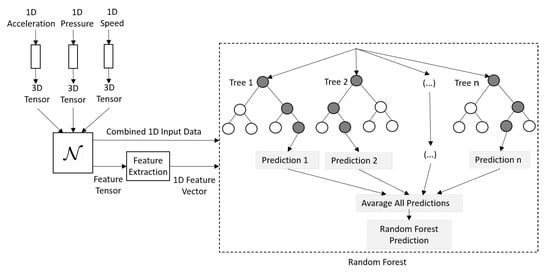
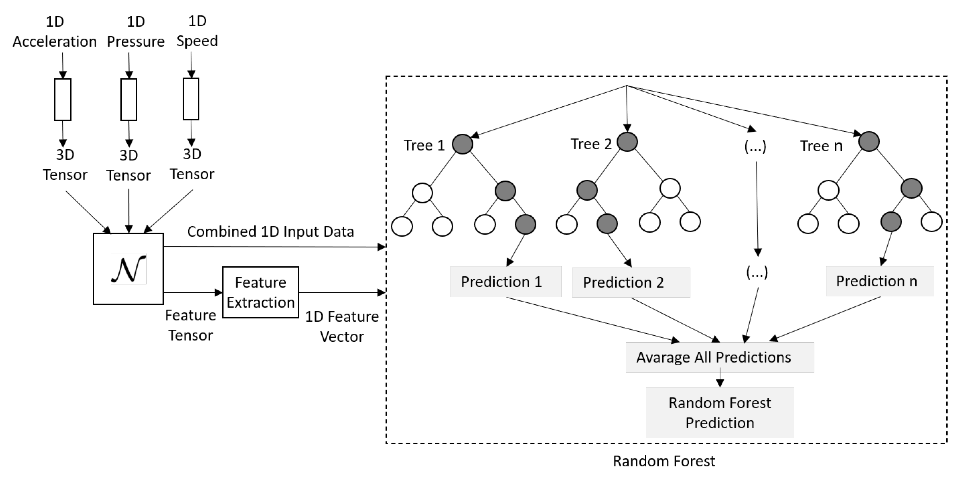
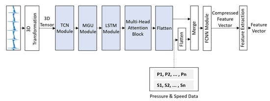
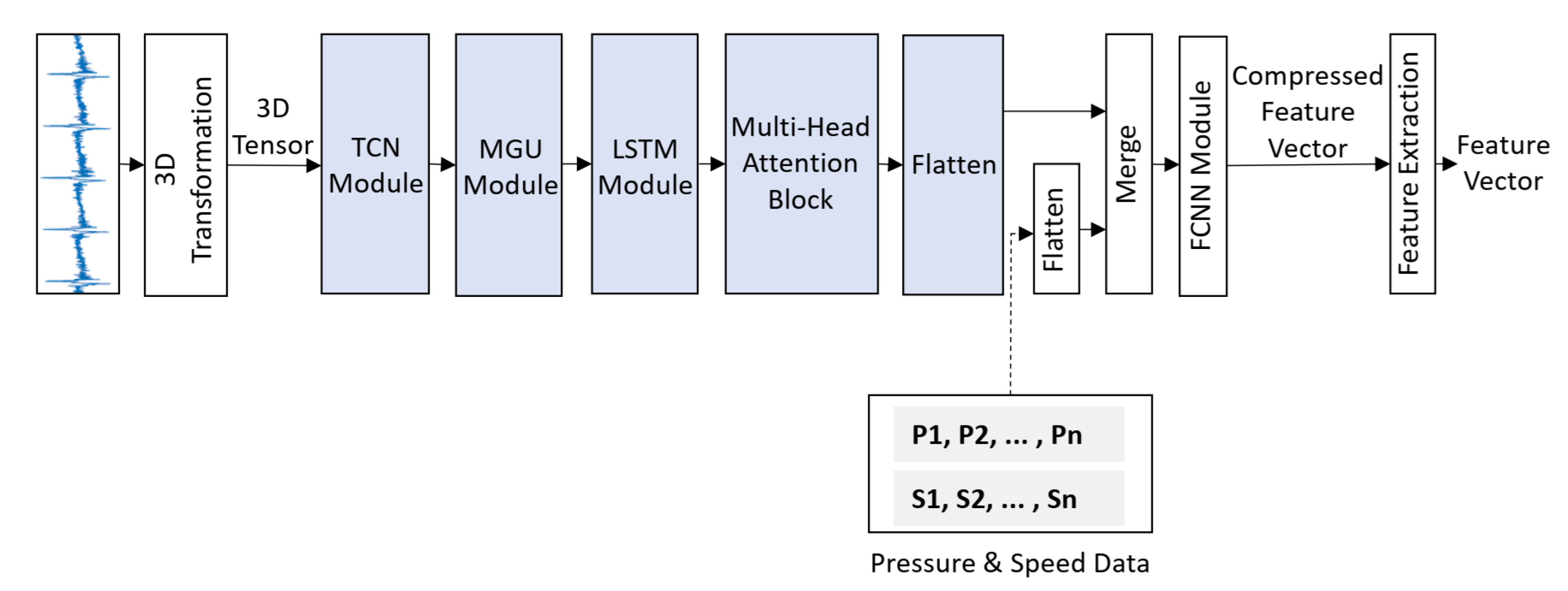
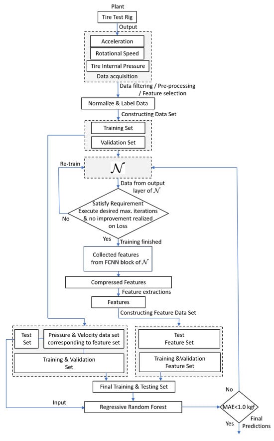
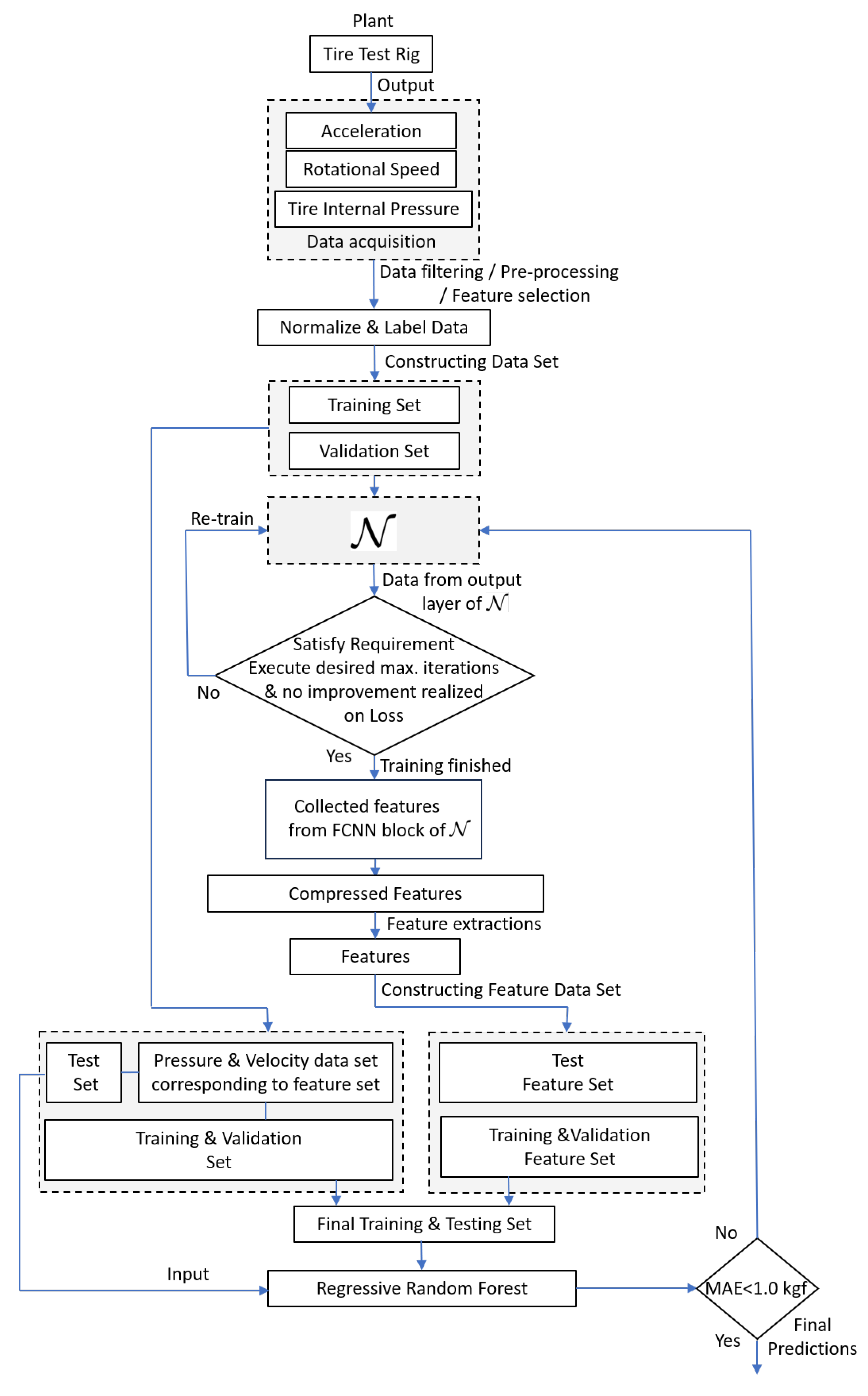
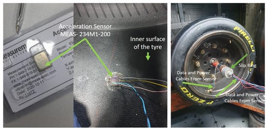
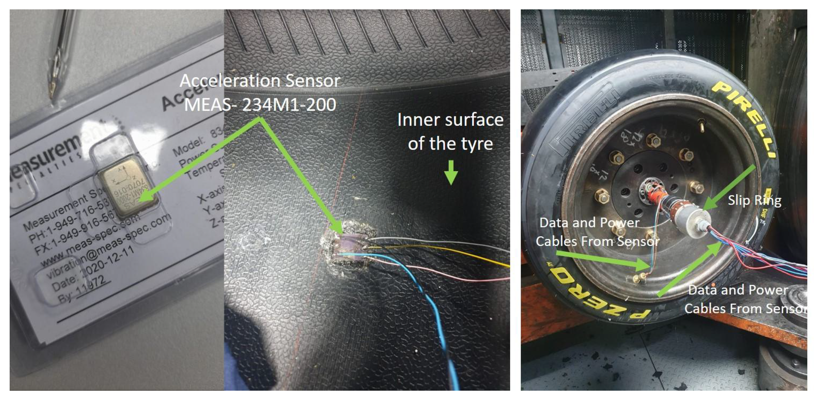
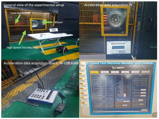
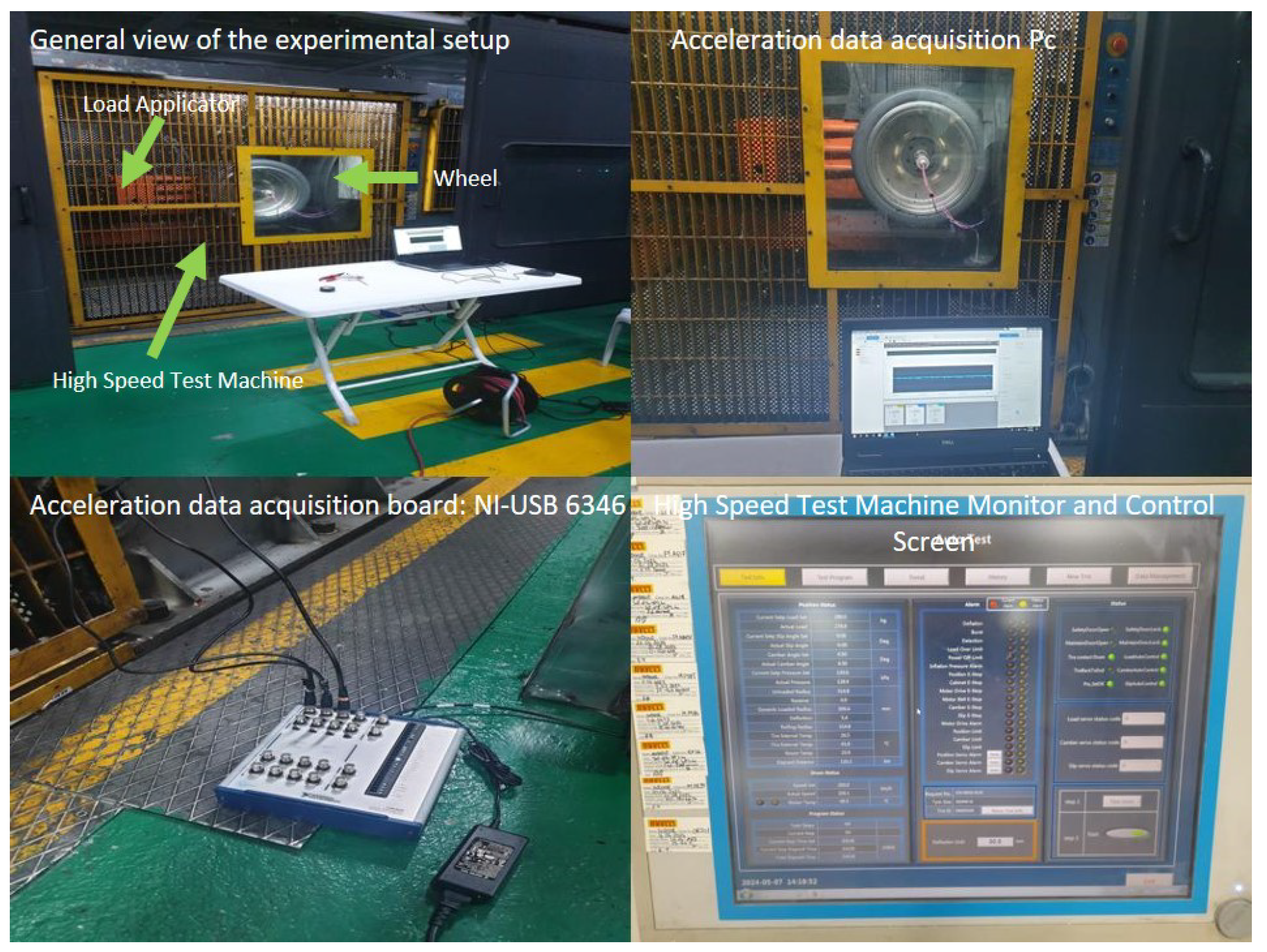
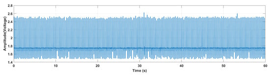
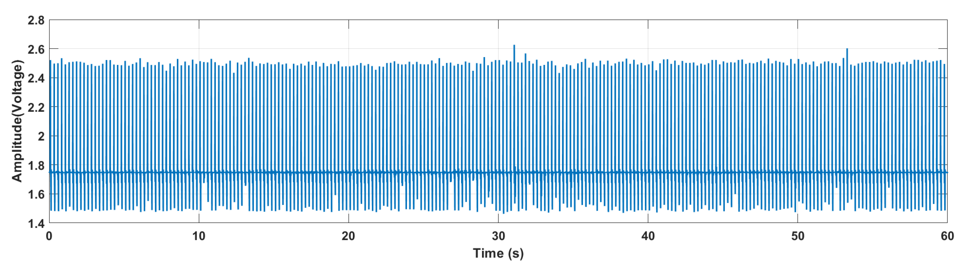
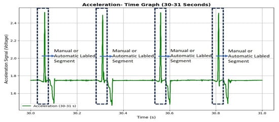
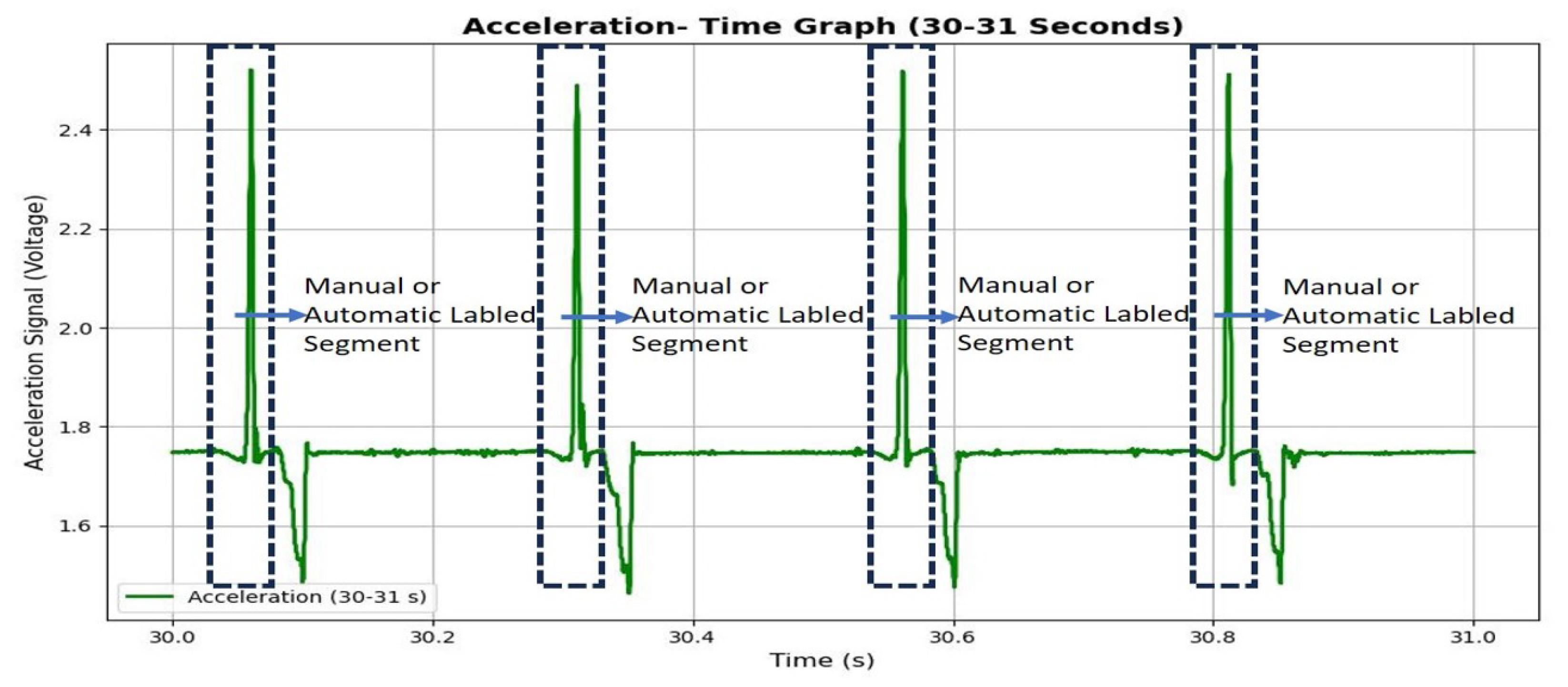
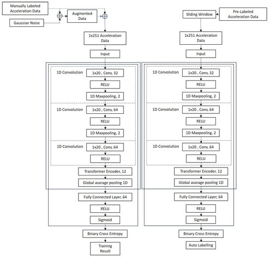
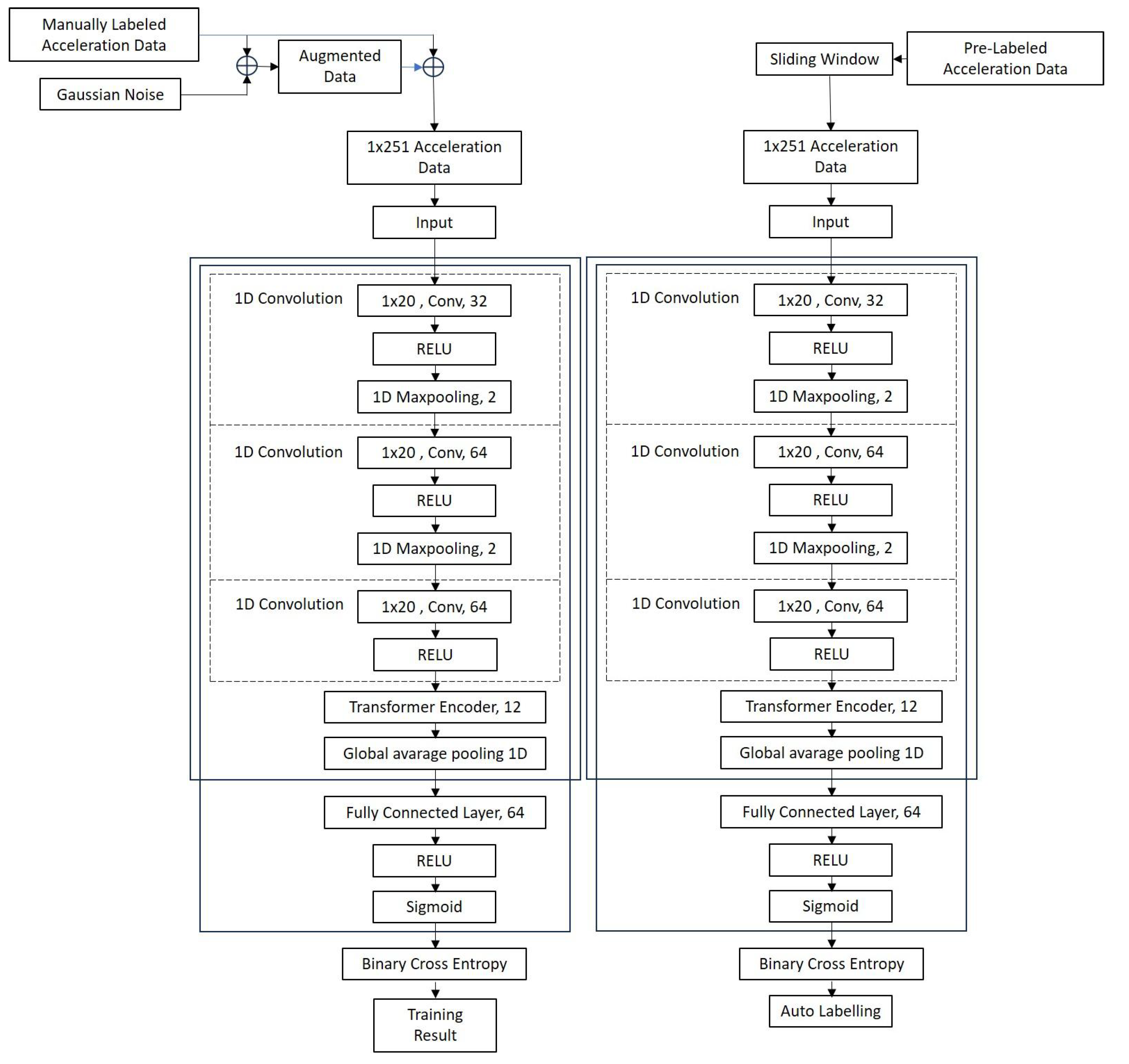
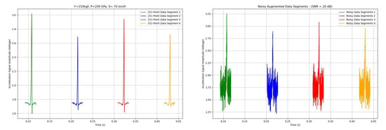
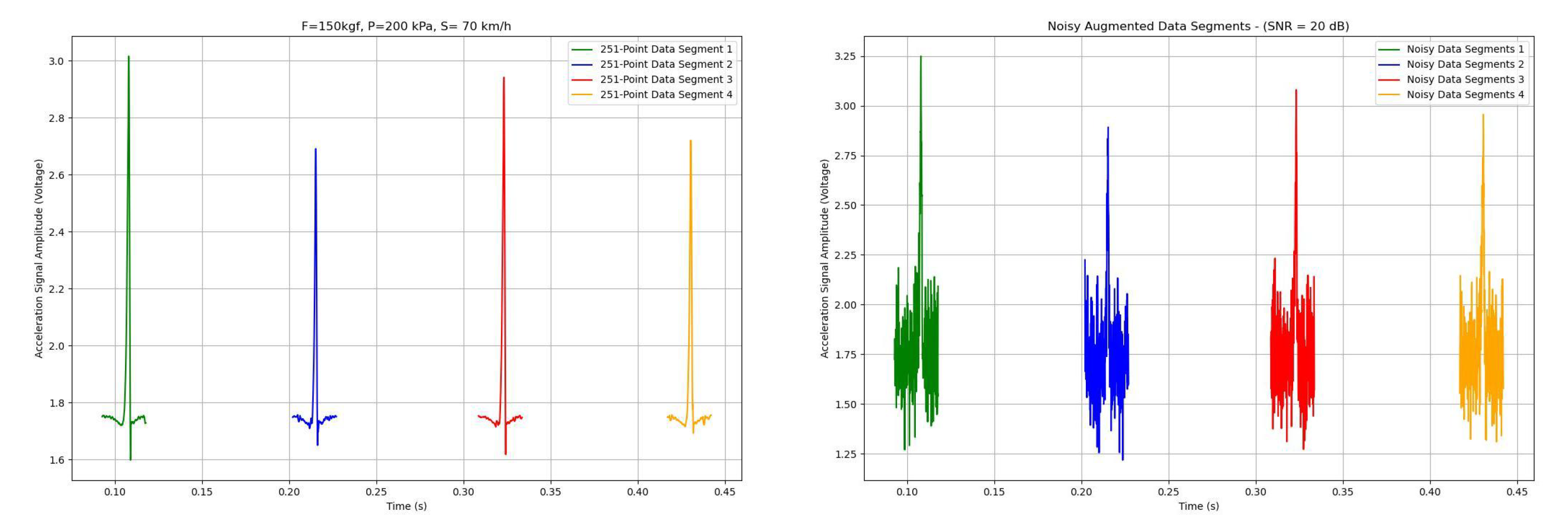
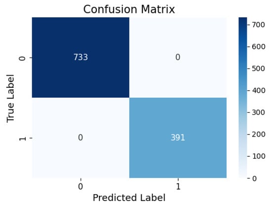
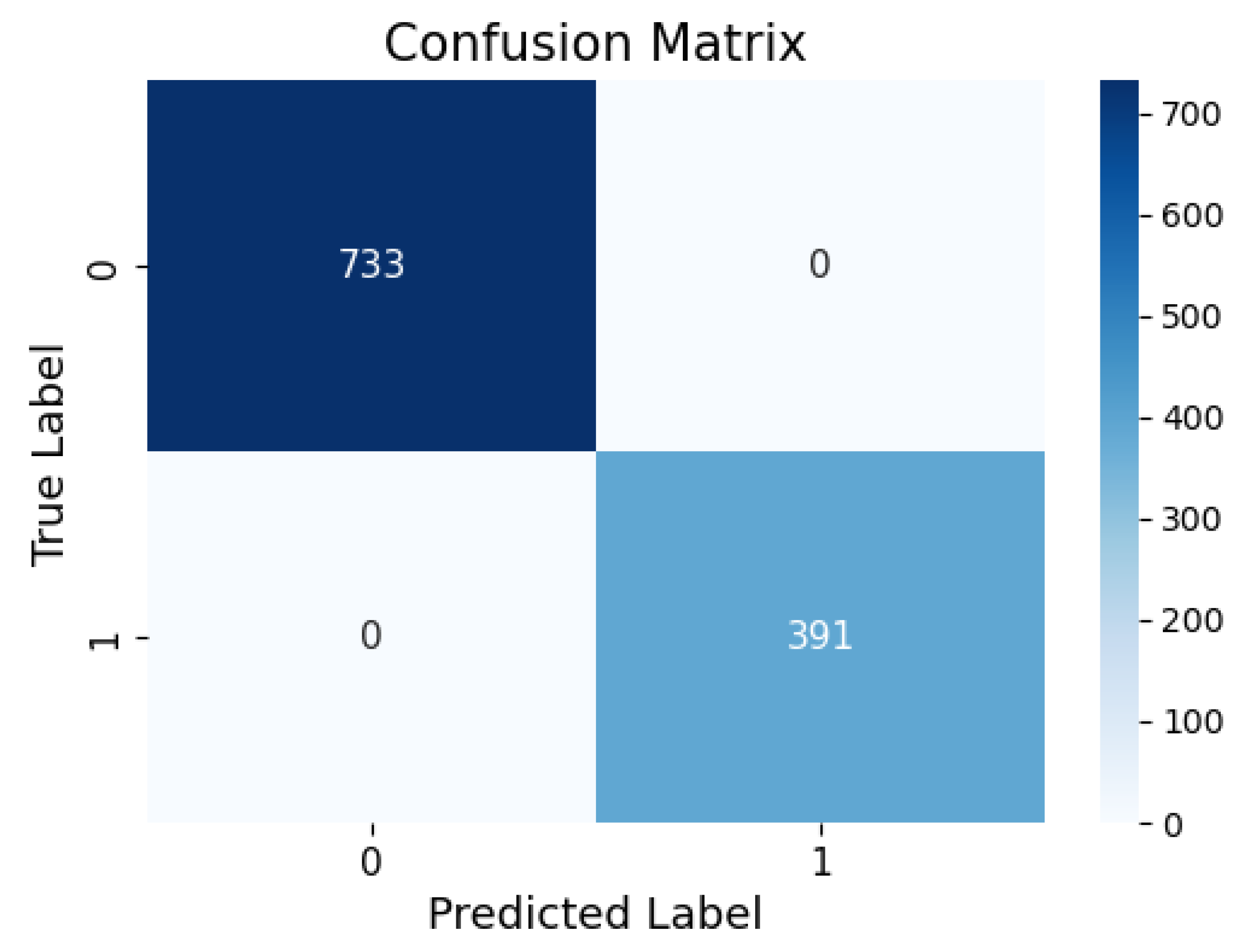
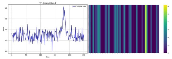
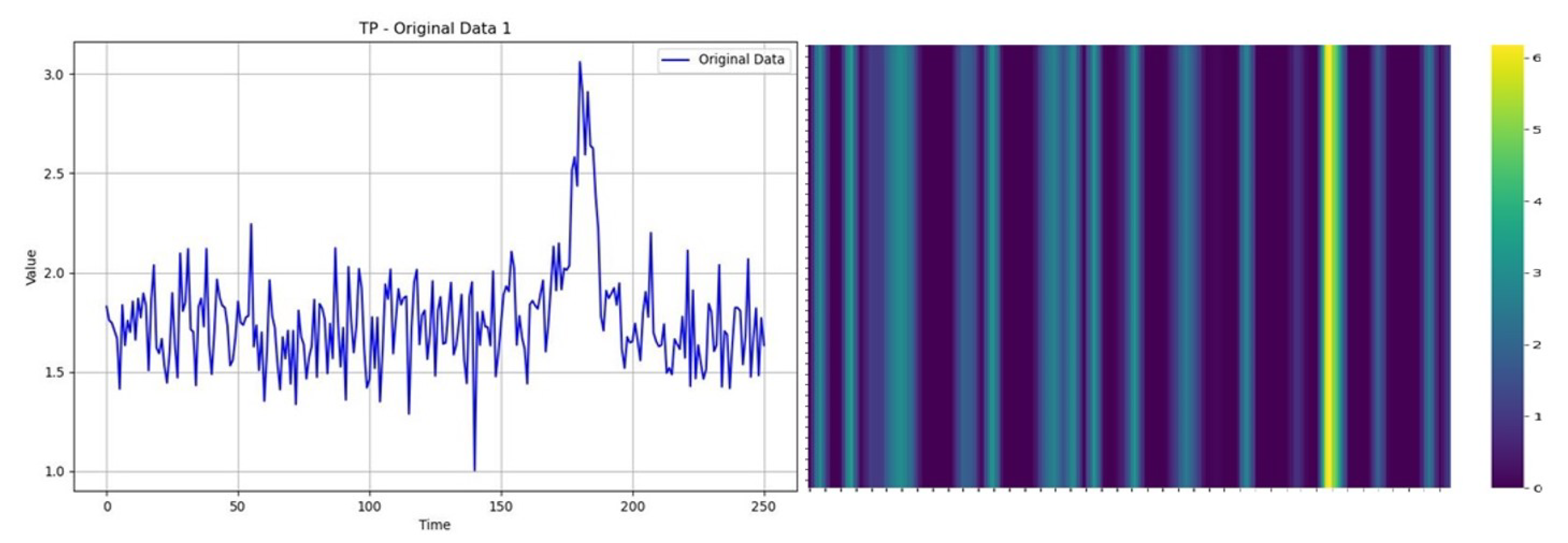
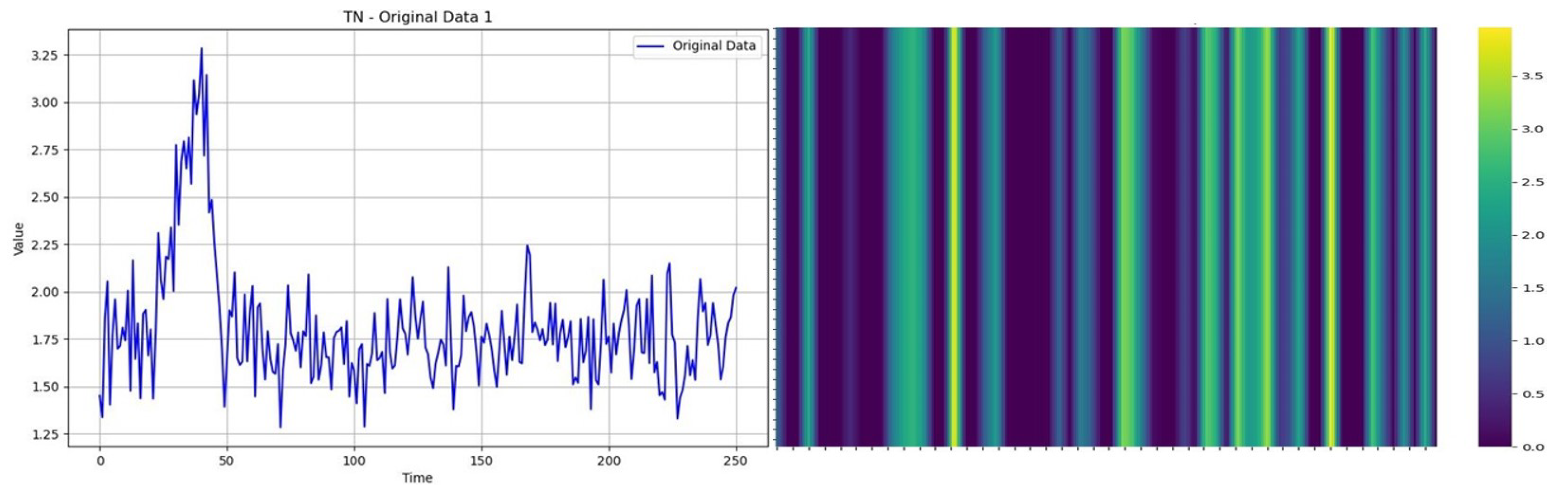
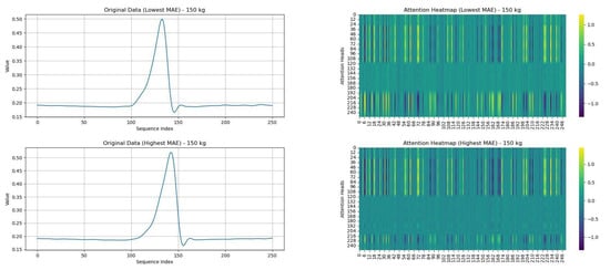
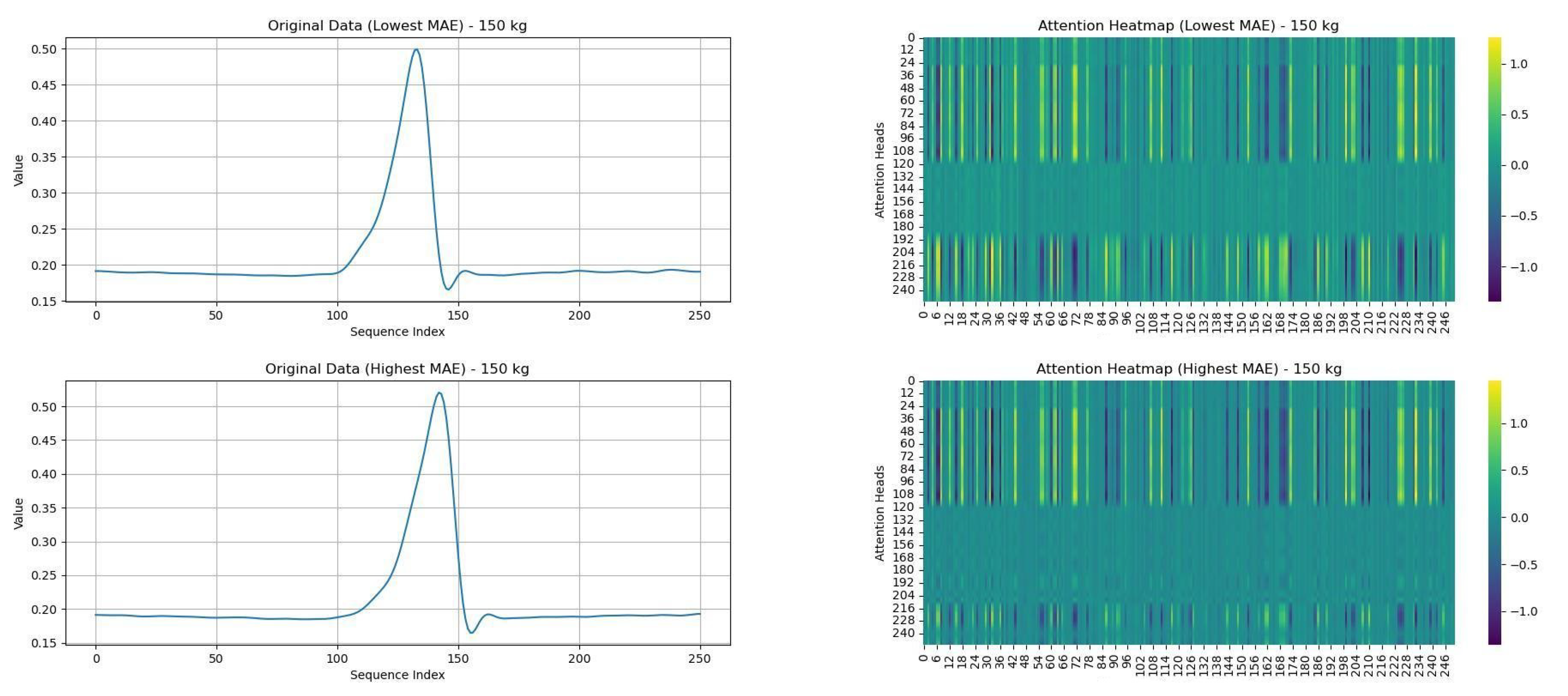
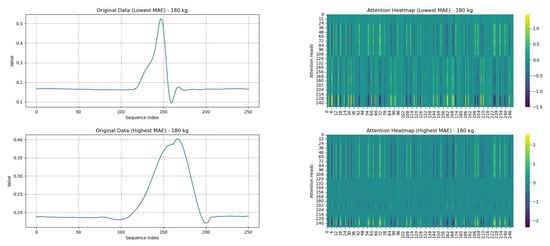
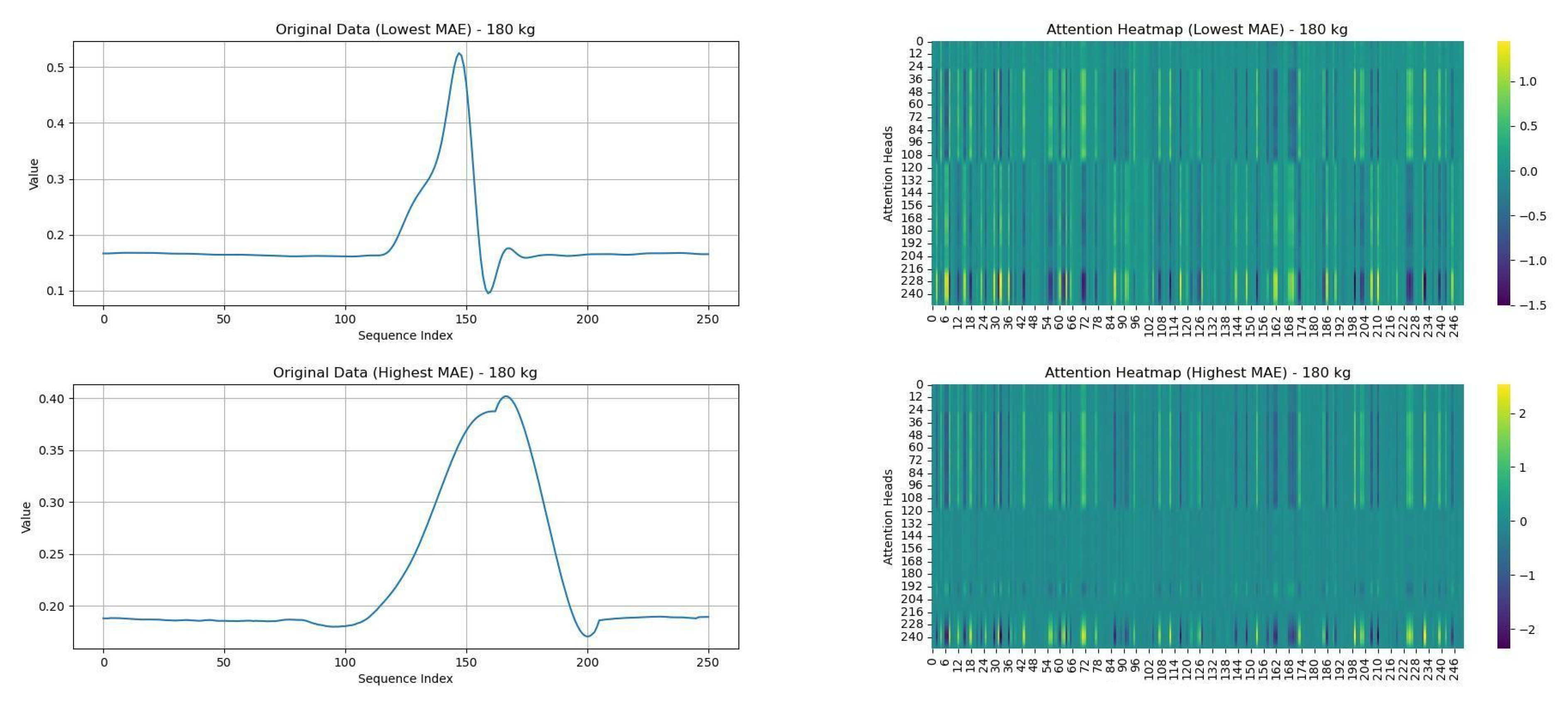
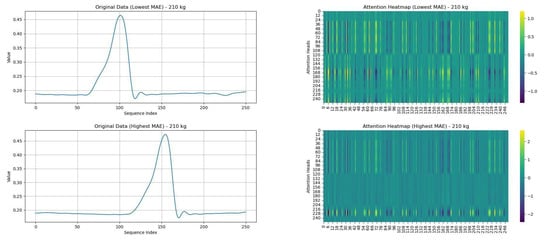
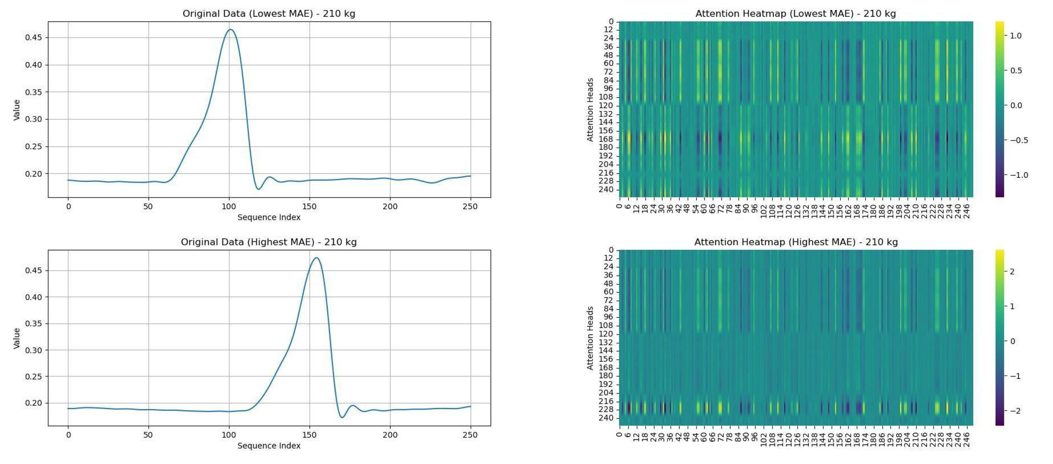
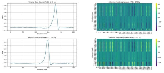
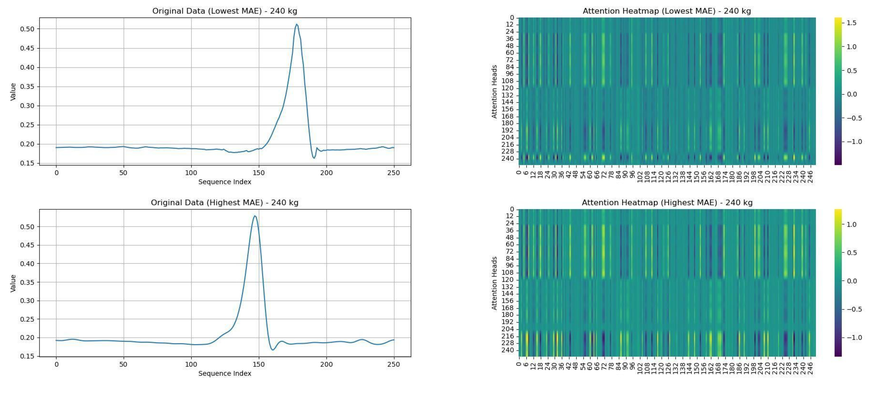
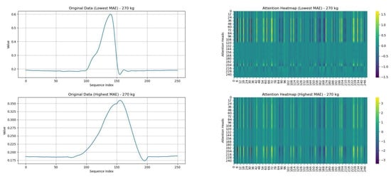
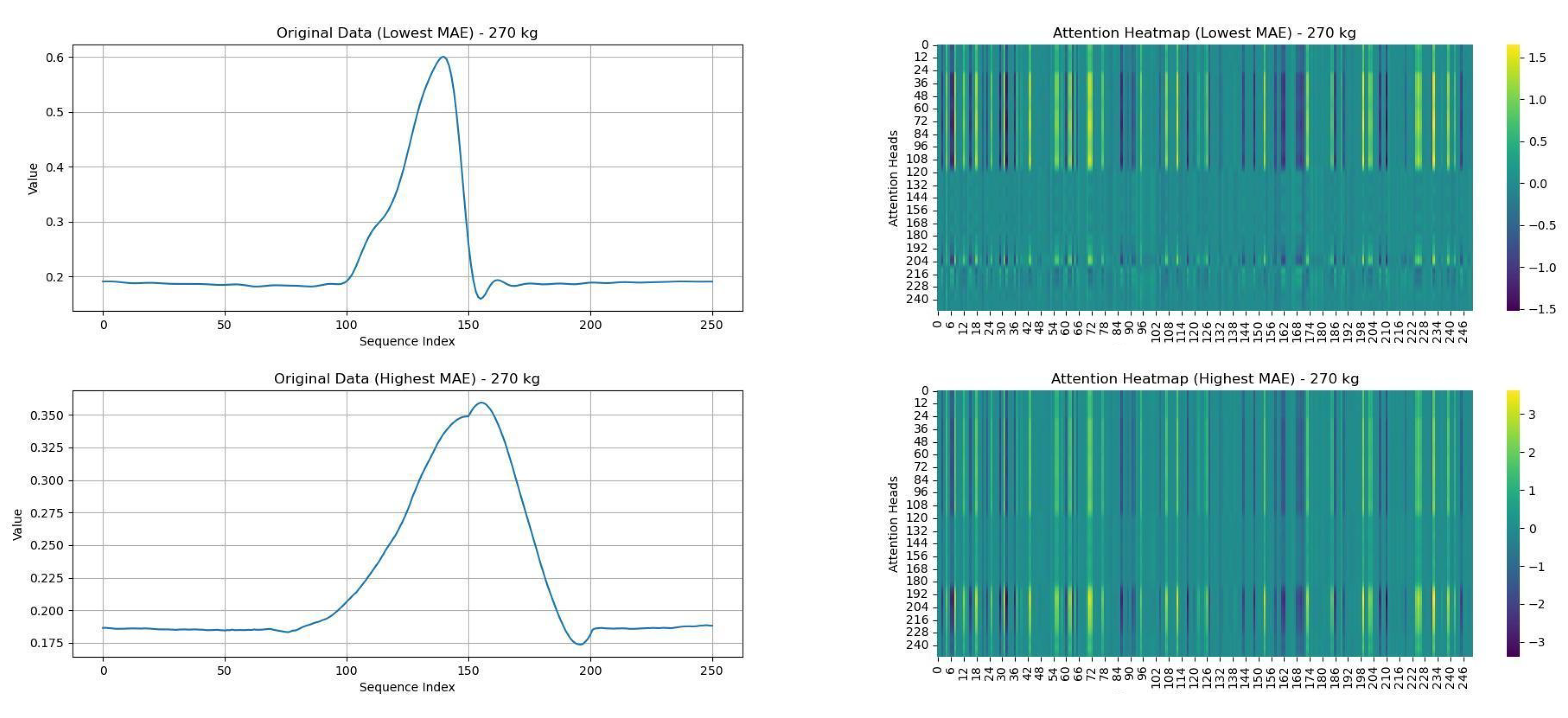
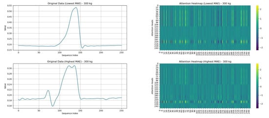
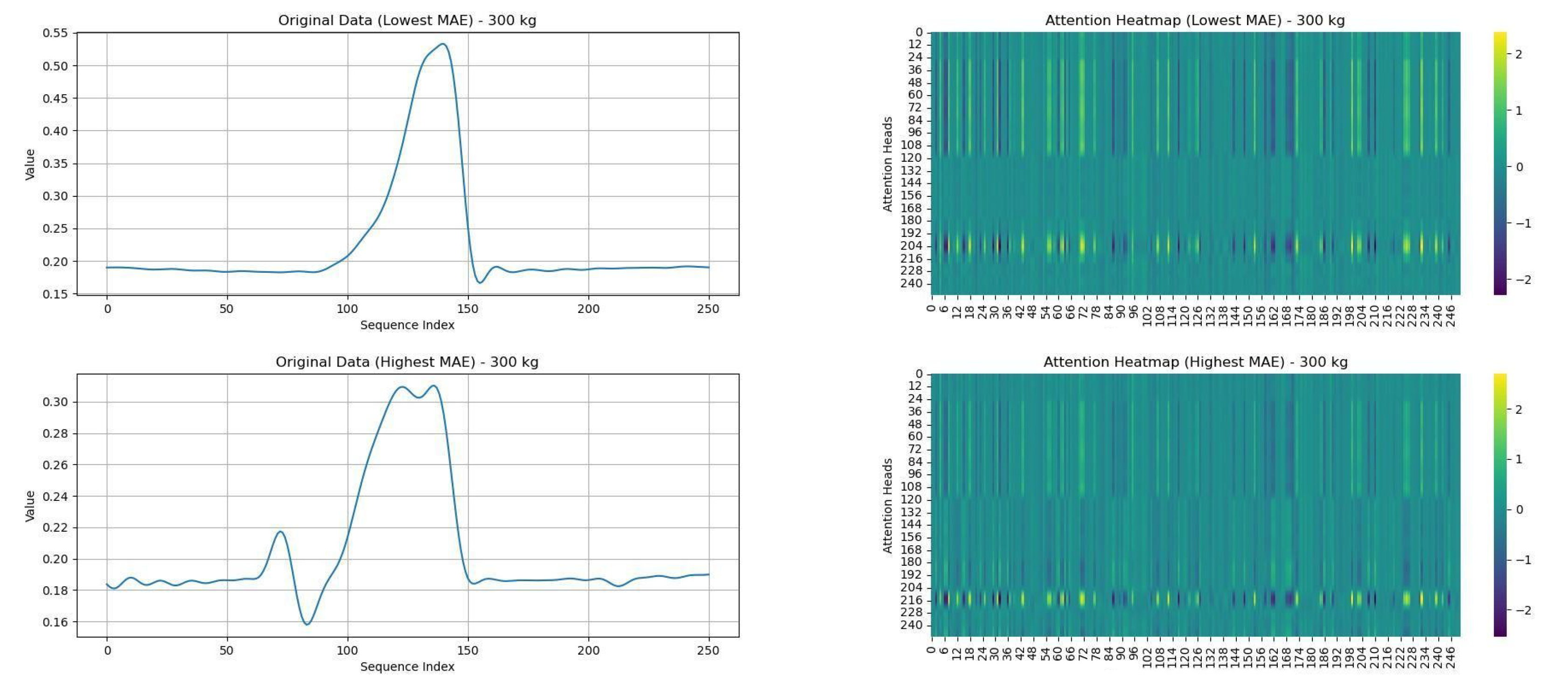
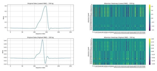
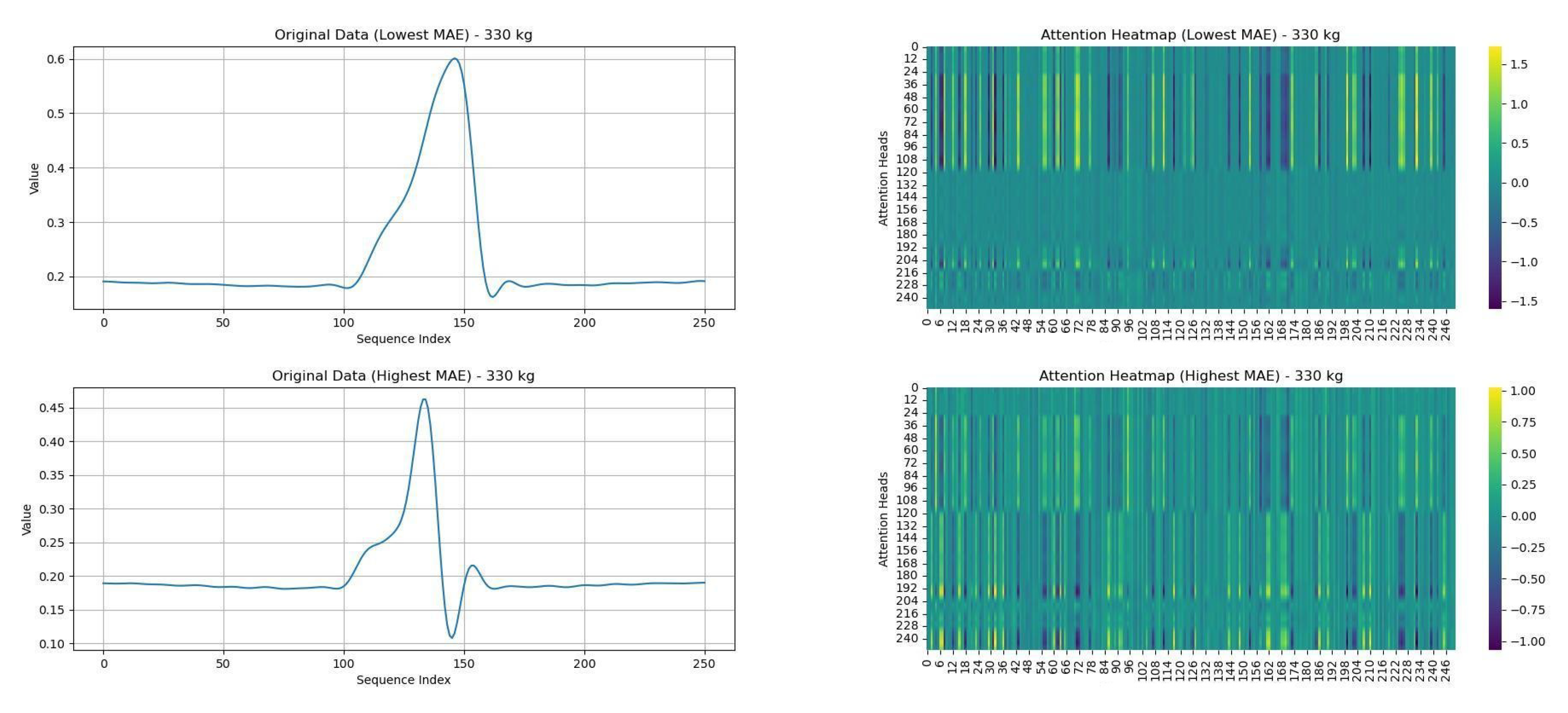
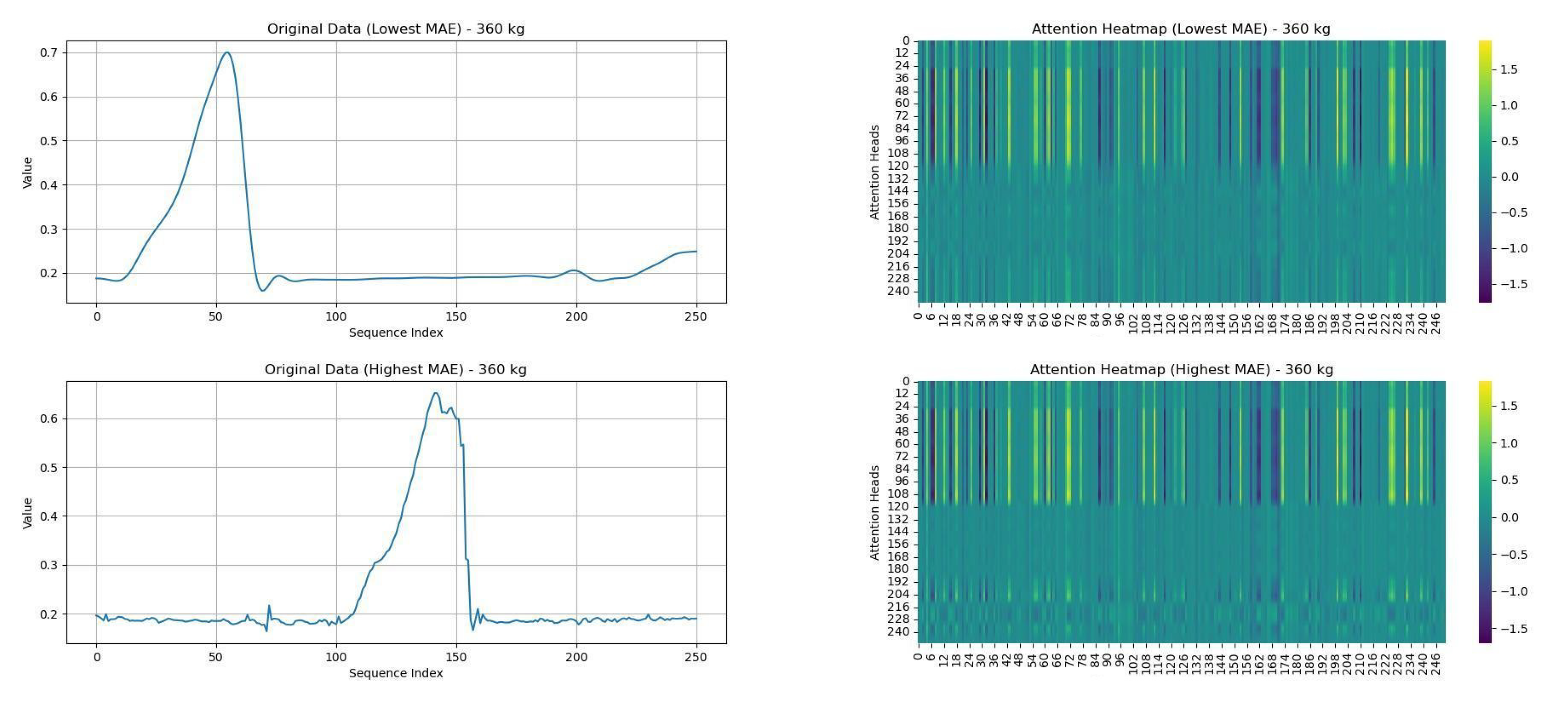
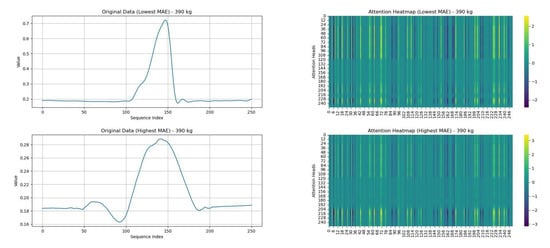
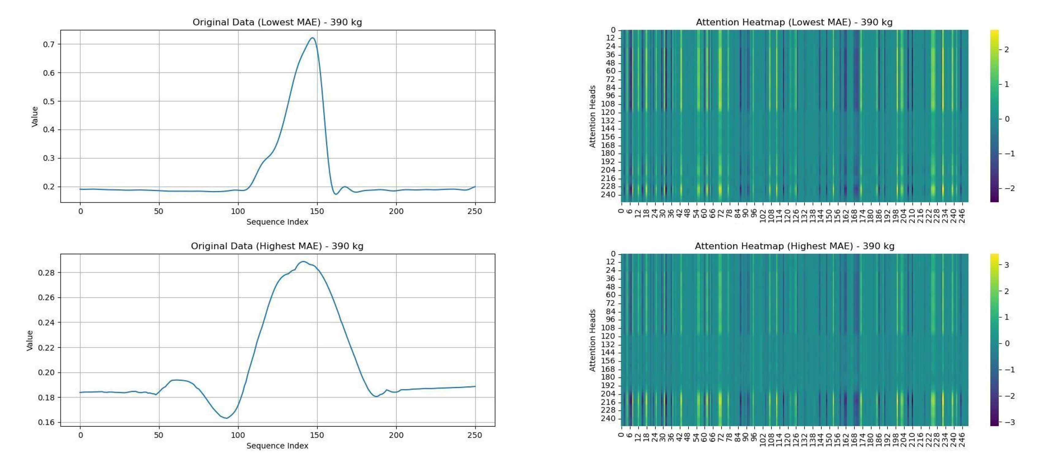
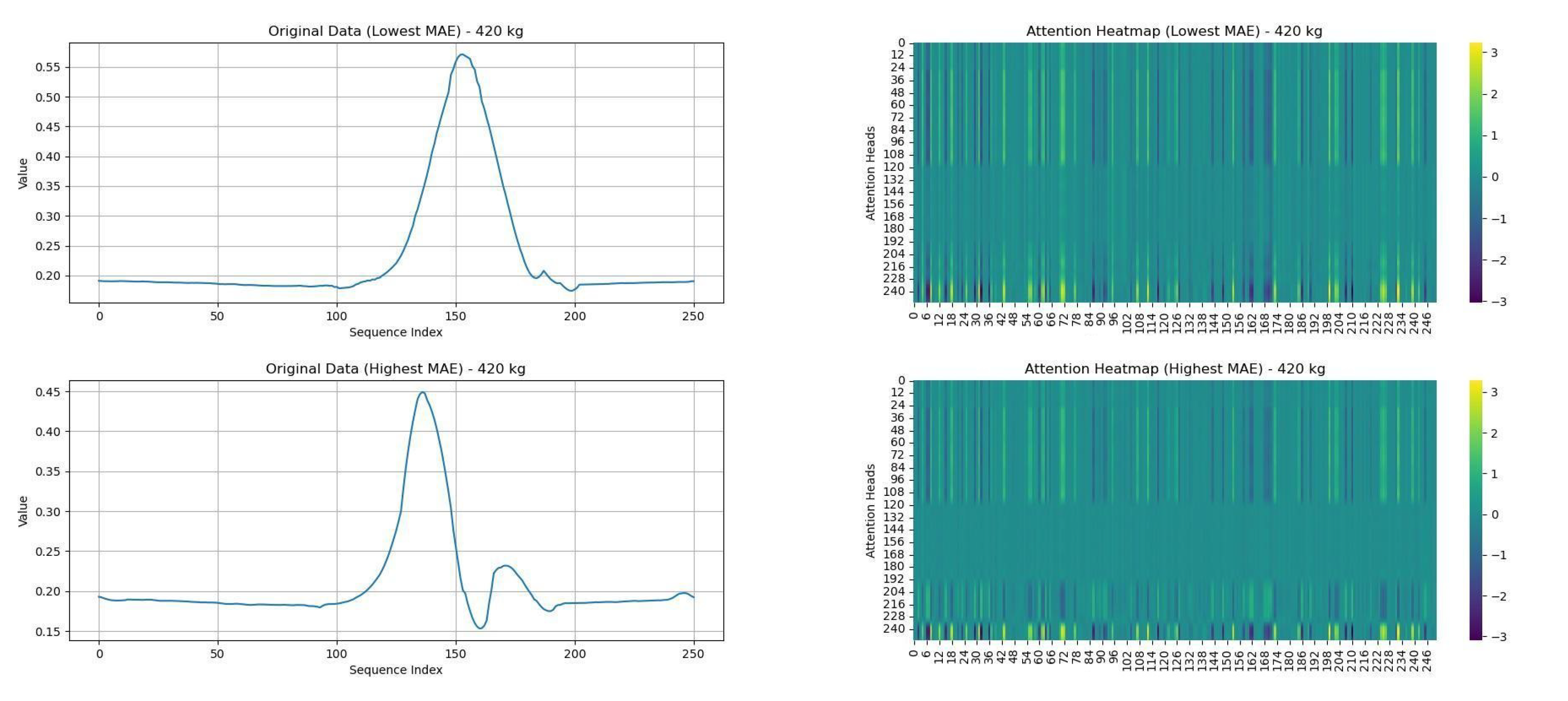
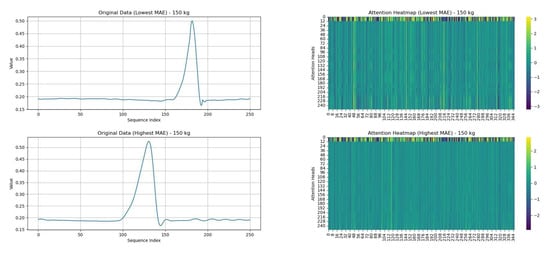
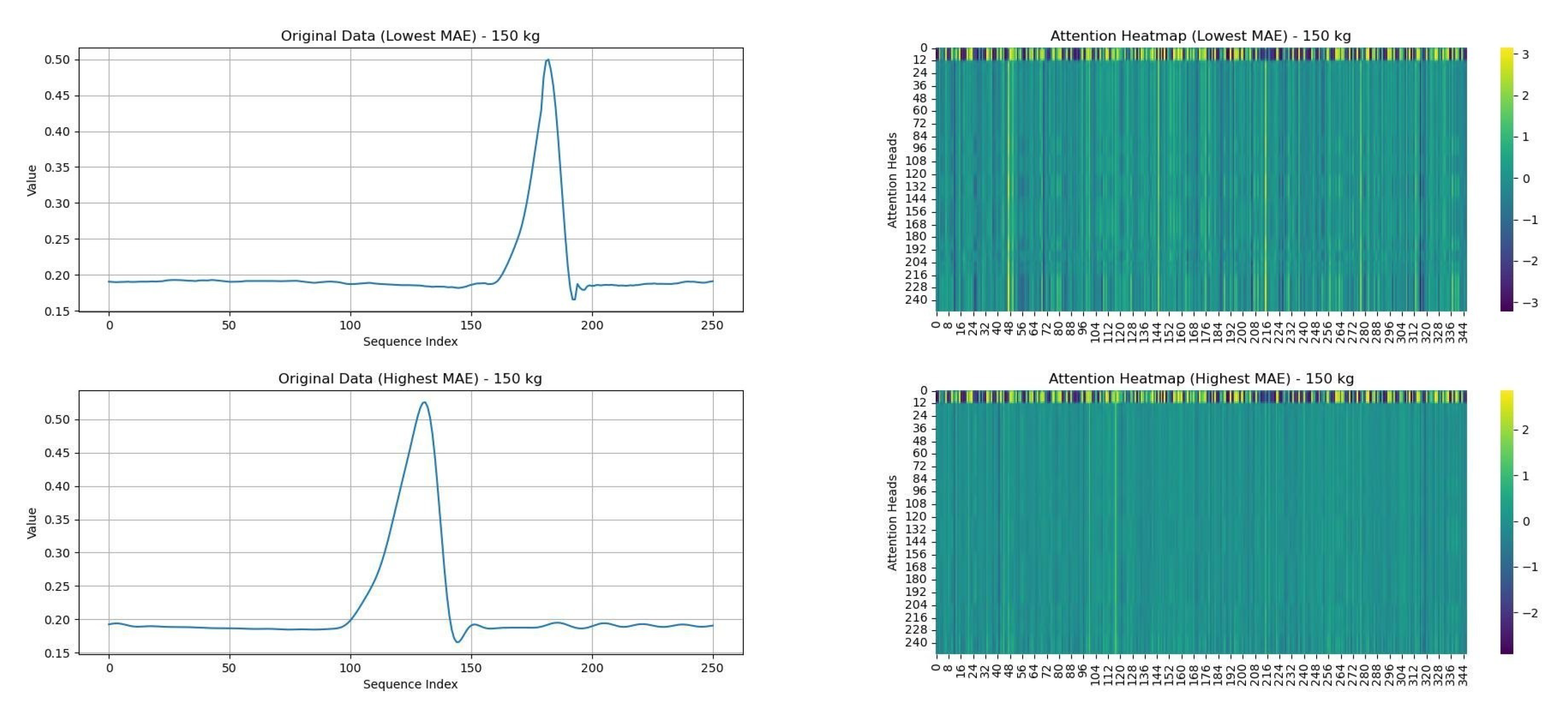
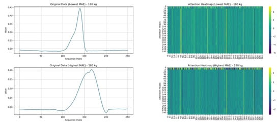
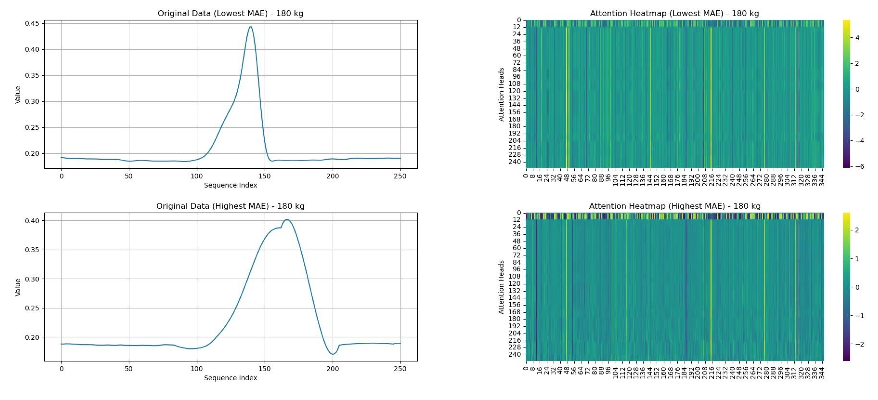
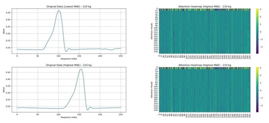
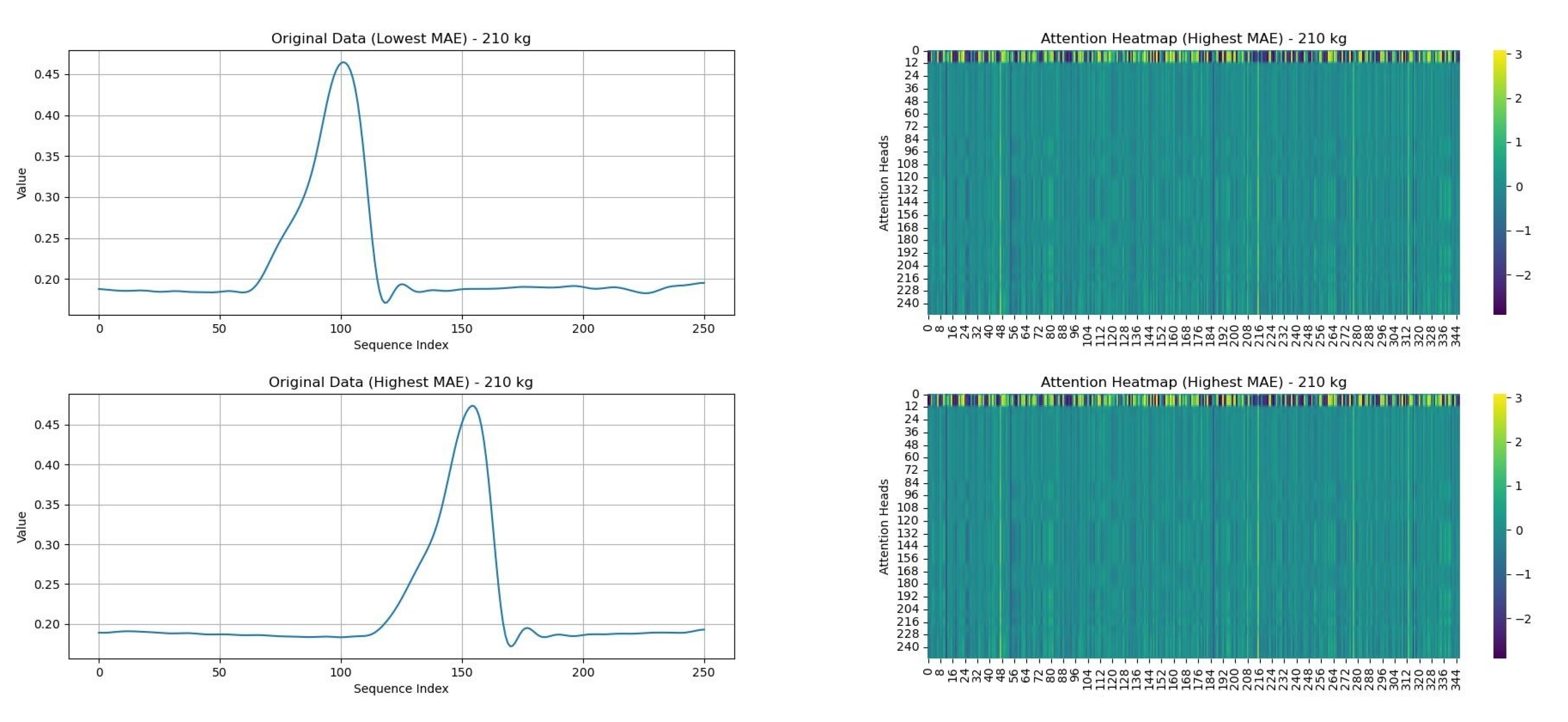
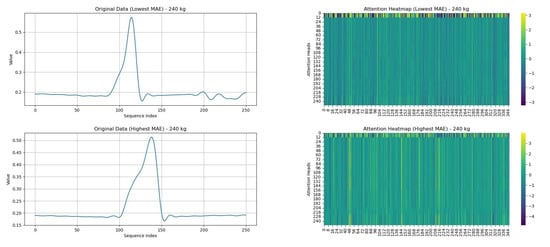
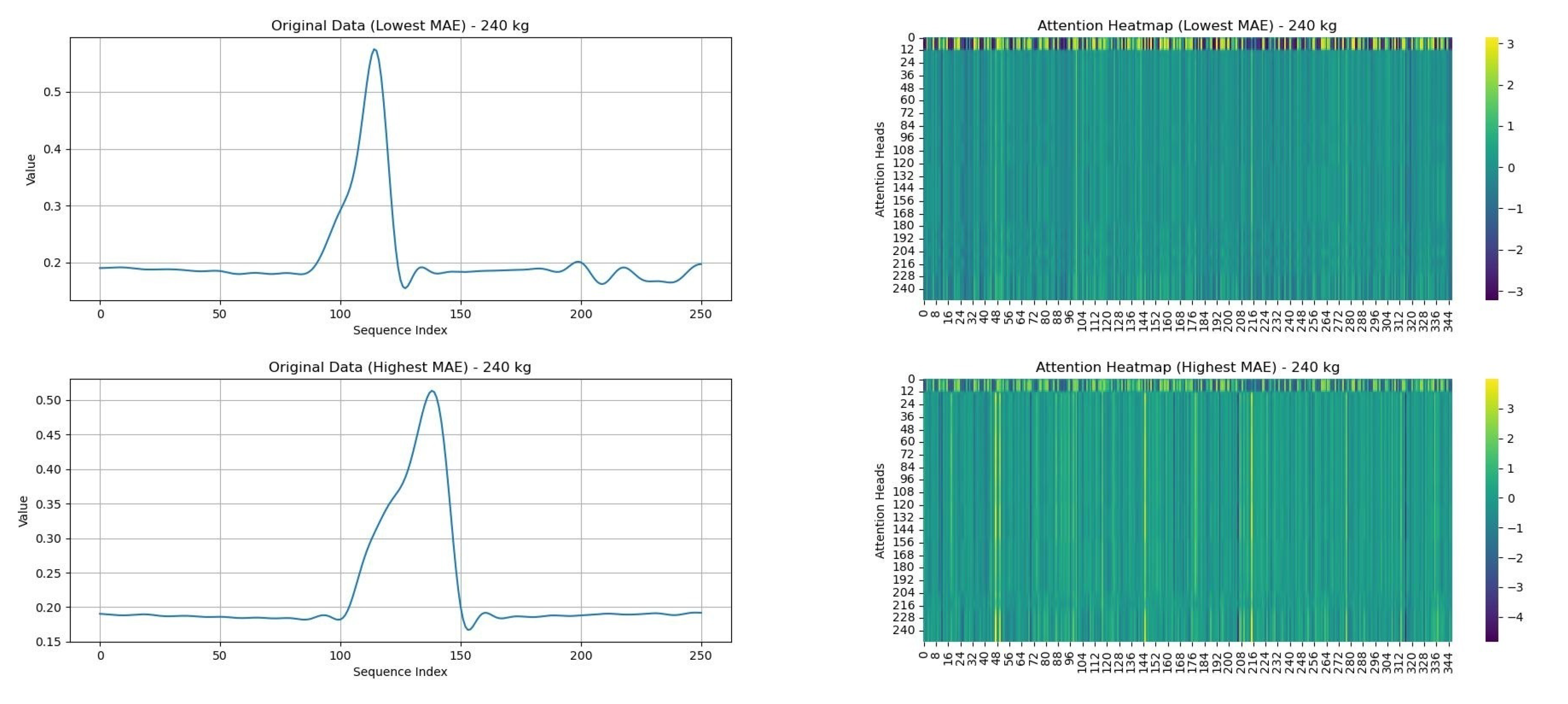
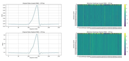
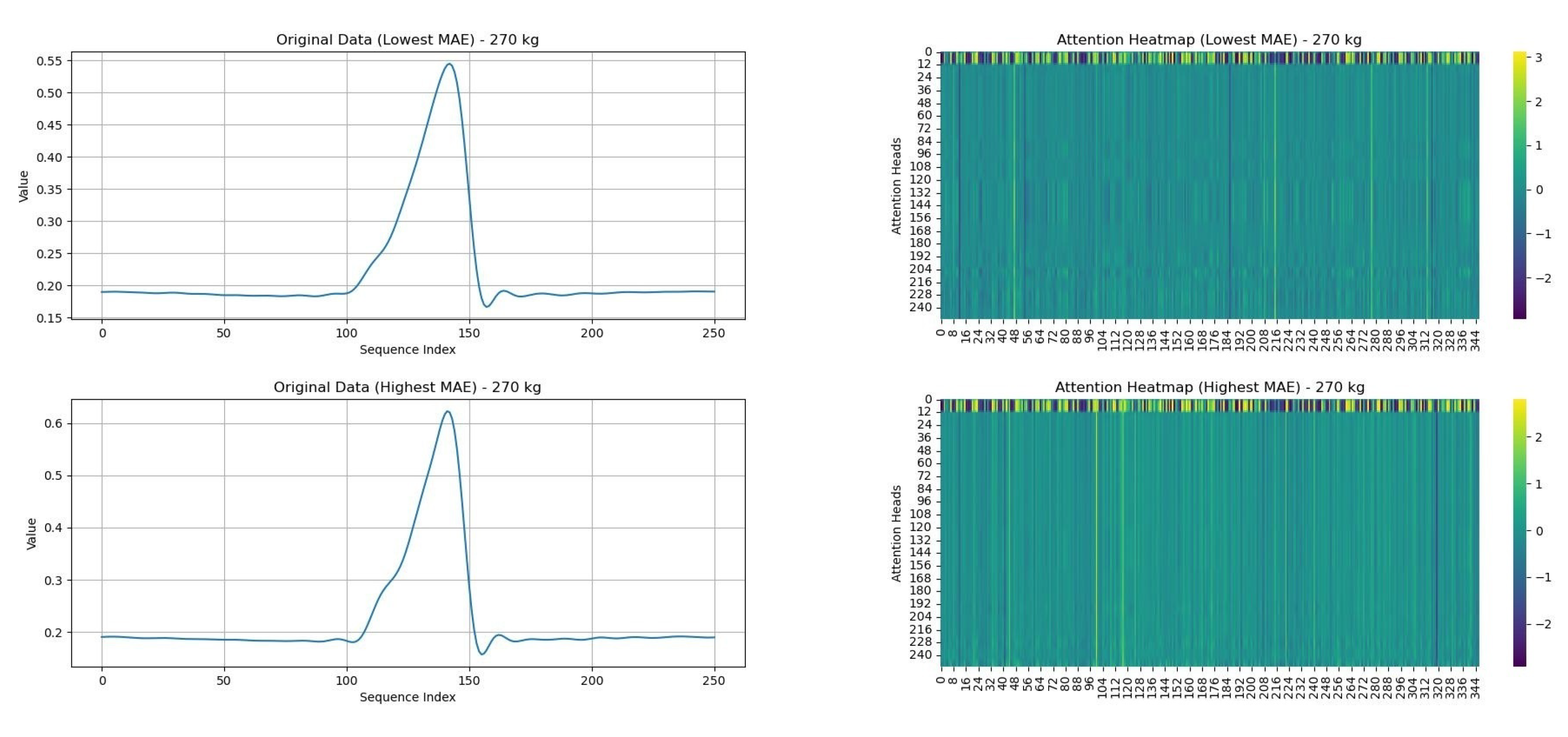
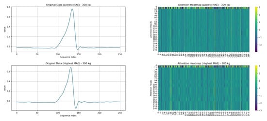
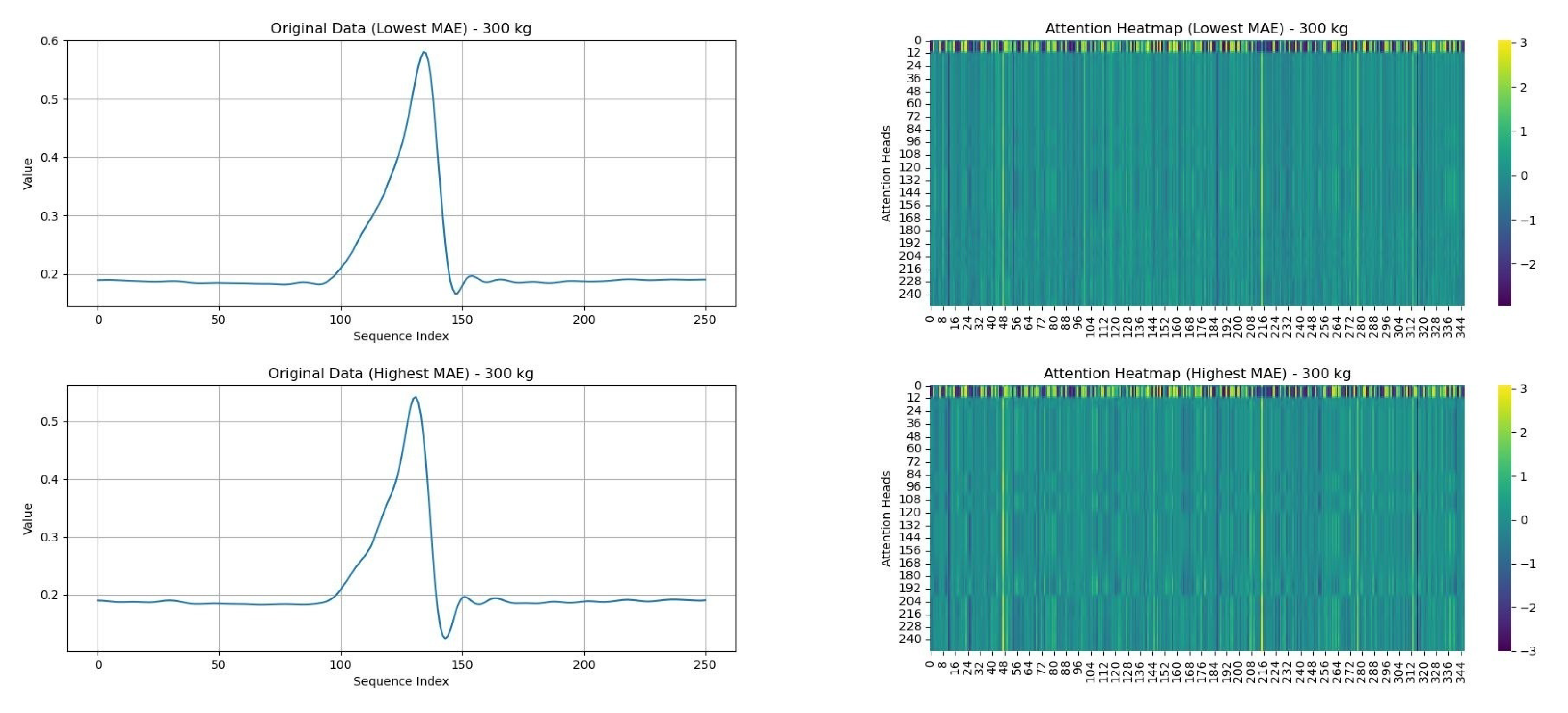
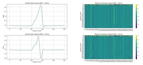
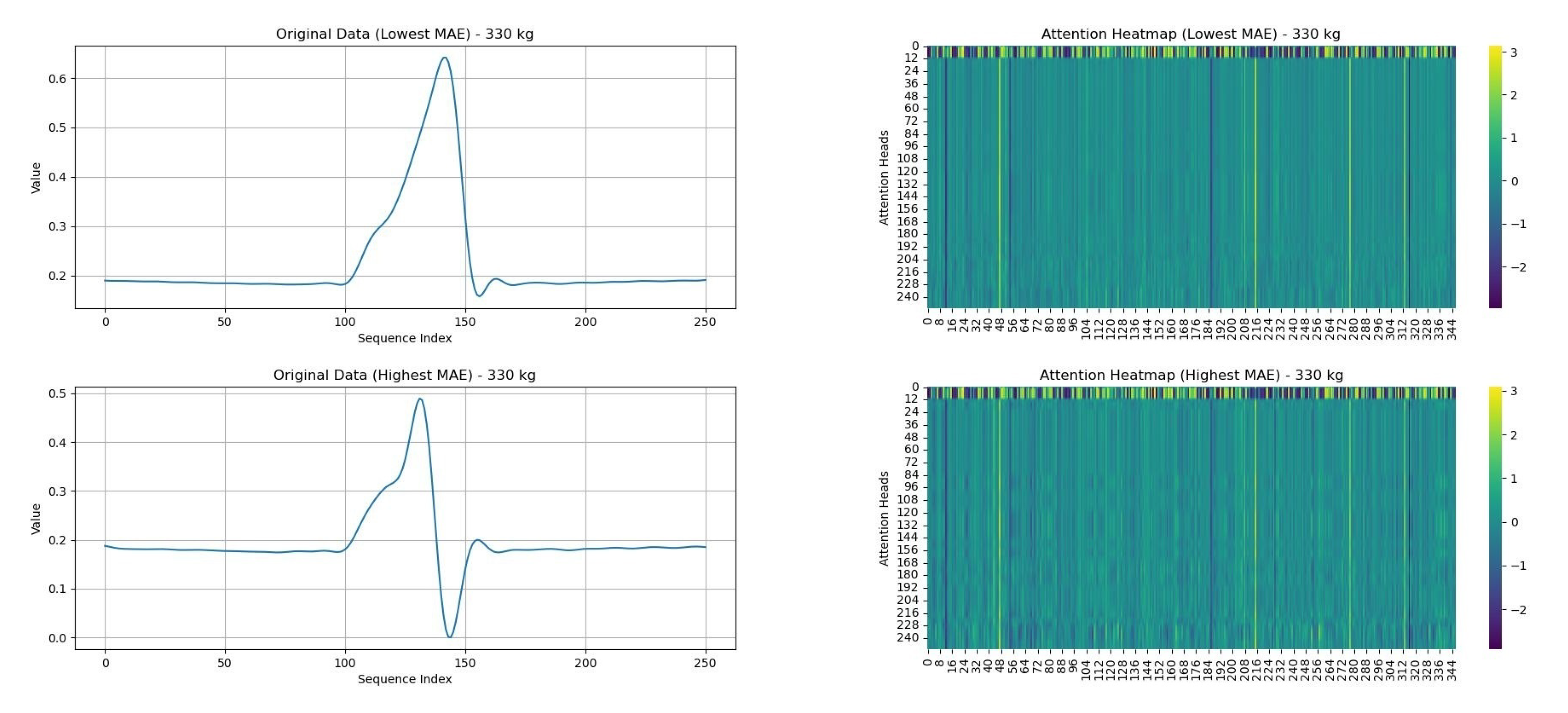
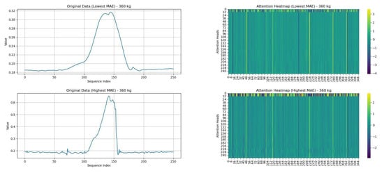
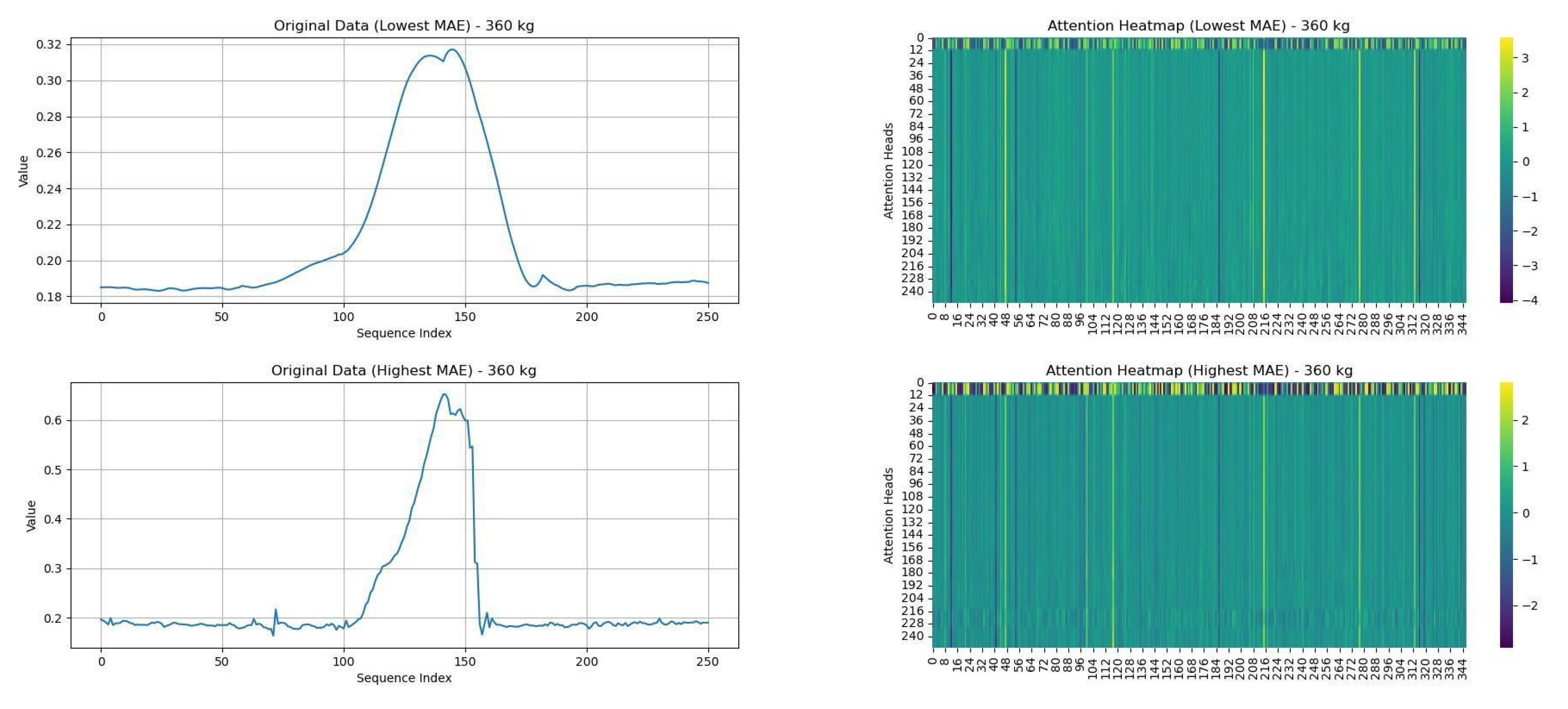
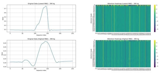
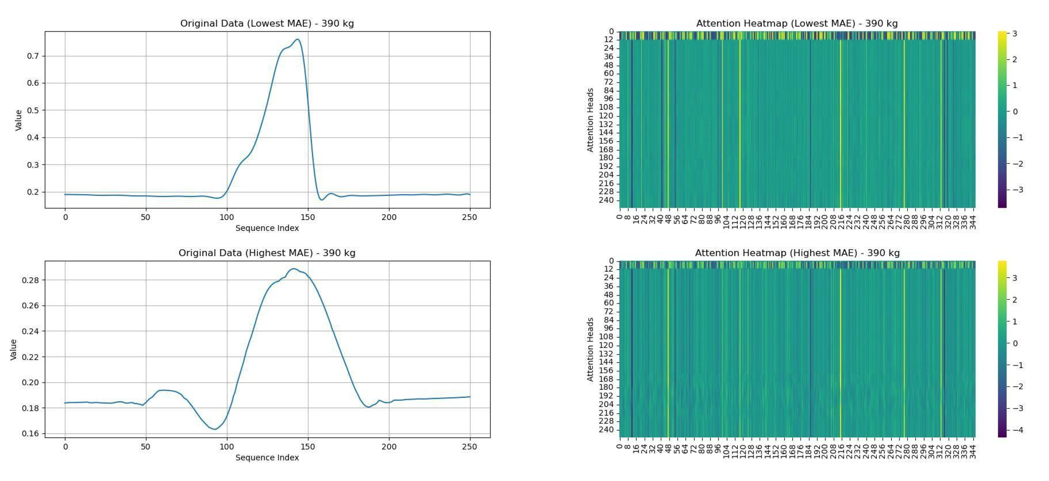
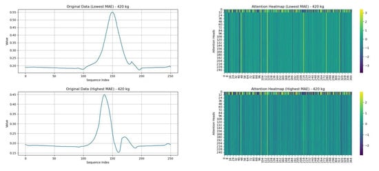
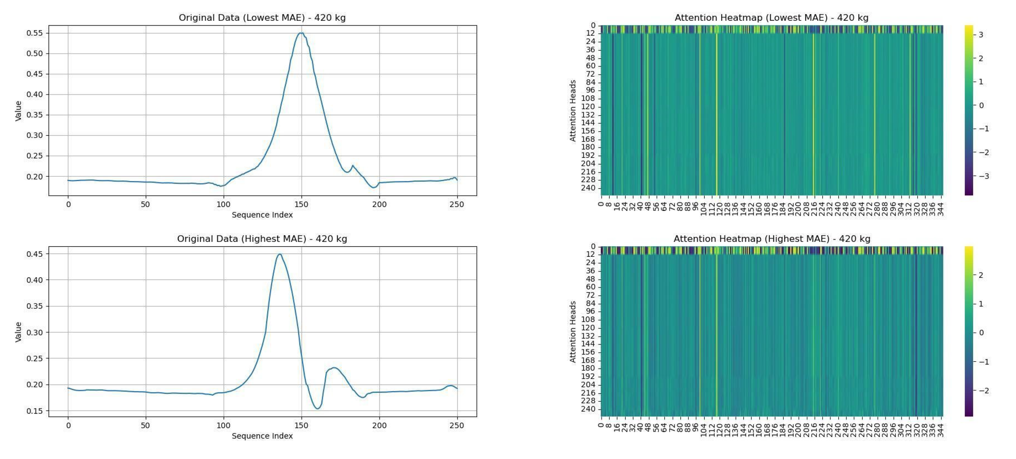
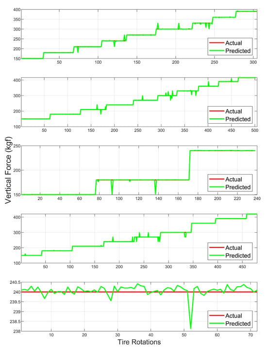
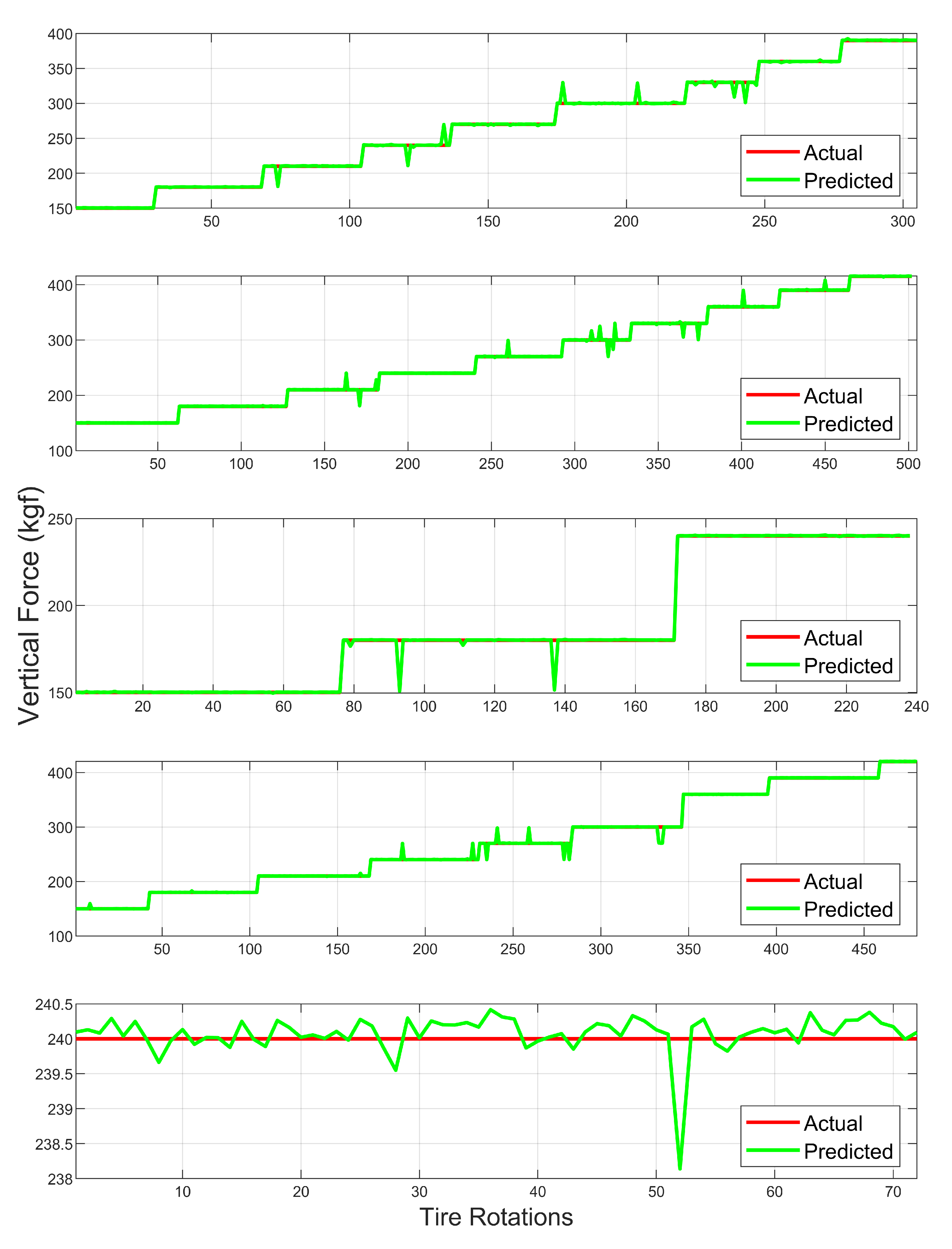

Disclaimer/Publisher’s Note: The statements, opinions and data contained in all publications are solely those of the individual author(s) and contributor(s) and not of MDPI and/or the editor(s). MDPI and/or the editor(s) disclaim responsibility for any injury to people or property resulting from any ideas, methods, instructions or products referred to in the content. |
© 2024 by the authors. Licensee MDPI, Basel, Switzerland. This article is an open access article distributed under the terms and conditions of the Creative Commons Attribution (CC BY) license (https://creativecommons.org/licenses/by/4.0/).