


Abstract
This paper proposes the “ultimate compression” method as a solution to the expansive computation and high storage costs required by state-of-the-art neural network models in inference. Our approach uniquely combines tensor decomposition techniques with binary neural networks to create efficient deep neural network models optimized for edge inference. The process includes training floating-point models, applying tensor decomposition algorithms, binarizing the decomposed layers, and fine tuning the resulting models. We evaluated our approach in various state-of-the-art deep neural network architectures on multiple datasets, such as MNIST, CIFAR-10, CIFAR-100, and ImageNet. Our results demonstrate compression ratios of up to 169×, with only a small degradation in accuracy (1–2%) compared to binary models. We employed different optimizers for training and fine tuning, including Adam and AdamW, and used norm grad clipping to address the exploding gradient problem in decomposed binary models. A key contribution of this work is a novel layer sensitivity-based rank selection algorithm for tensor decomposition, which outperforms existing methods such as random selection and Variational Bayes Matrix Factorization (VBMF). We conducted comprehensive experiments using six different models and present a case study on crowd-counting applications, demonstrating the practical applicability of our method. The ultimate compression method outperforms binary neural networks and tensor decomposition when applied individually in terms of storage and computation costs. This positions it as one of the most effective options for deploying compact and efficient models in edge devices with limited computational resources and energy constraints.
Keywords:
DNN; tensor decomposition; pruning; efficient DNN; quantization; binary neural network; edge AI 1. Introduction
Deep neural networks have shown exceptional performance in various fields of machine learning, including computer vision, speech recognition, and natural language processing [1]. In particular, Convolutional Neural Networks (CNNs) have demonstrated significant performance in computer vision tasks such as image recognition, object detection, and image segmentation [2]. The availability of ample training data and advanced computation hardware and the use of Graphical Processing Units (GPUs) make training and deployment of deep CNN models feasible [3].
Deep CNN models usually consist of many layers that contain millions or hundreds of trainable parameters. This large number of parameters requires high storage and computation capacities [3,4]. Deploying these models is challenging, especially for low-energy-constrained devices such as mobile devices, Internet of Things (IoT) nodes, CPU robotics, or autonomous vehicles [5,6]. To address this issue, various software and hardware methods have been introduced in recent years to compress these models and accelerate the training and inference stages of deep neural network models.
In this paper, we apply three tensor decomposition methods, namely CP decomposition (also known as CANDECPMP or PARAFAC), Tucker decomposition, and tensor train decomposition, to a version of a binary neural network called XNOR-Net to reduce the memory footprint of these models and decrease their computational cost. After applying tensor decomposition methods to XNOR-Net models, we obtain the same accuracy performance for LeNet-5 and Network in Network (NIN) models, with a small degradation of accuracy for deeper models such as Alexnet, Resnet-20, and Resnet-32. Overall, our method significantly reduces the number of learnable parameters in both models compared to their floating-point models.
Our method combines and studies tensor decomposition with quantization; this combination has not been studied or explored before to this extent. This combination not only minimizes the storage requirements but also makes the deep learning models easy to deploy on the edge. The reduction in computational complexity also translates to lower power consumption, which can be beneficial for power-constrained or energy-harvested edge systems. Our method effectively balances performance and resource utilization, which ensures its practicality for edge computing applications.
Beyond general edge computing, our work has promising applications in the domain of vehicular networks, where resource optimization and data security are the primary objectives. Ying Ju et al. proposed the use of NOMA-assisted secure offloading, which improves the efficiency and security of vehicular edge computing networks by using asynchronous deep learning and reinforcement learning to manage offloading decisions in real-time environments [7]. However, this method often struggles to balance computational load with latency and energy consumption, especially when deployed on heterogeneous edge devices. Our method offers a complementary solution that reduces the computational and memory requirements for deep learning models, simplifying their deployment across a broad range of edge devices. Unlike other existing methods, our approach using ranking selection is more versatile than other ways, allowing it to be applied to a wide range of edge applications.
This approach also confirms the intuition that CNN models are over-parameterized [8]. A considerable number of trainable parameters is not required to store the classification task; instead, such parameters are needed for the optimization task, which can help models to converge to good local minima of the loss function [9]. In this paper, we apply tensor decomposition methods to floating-point deep neural network models, then binarize the models using a type of binary neural network called XNOR-Net [10].
The contributions of this paper are summarized as follows:
- We propose an efficient deep neural network model by applying the tensor decomposition method to Binary Neural Networks (BNNs).
- We introduce an algorithm for selecting the rank of the tensor to decompose the models based on the sensitivity of the layer for decomposition.
- We compare three methods for selecting the rank for decomposition, namely the random method; Variational Bayes Matrix Factorization (VBMF); and our method, which selects ranks based on layer sensitivity.
- We demonstrate the effectiveness of our method using six different models on four different datasets, namely LeNet-5 on MNIST; Network in Network, Alexnet, ResNet-20, and ResNet-32 on CIFAR-10; ResNet-20 and ResNet-32 on CIFAR-100; and, finally, Alexnet and Resnet-18 on ImageNet.
- We use a crowd-counting application as a case study for our method, using two different models (MCNN and CSRNet) and four different datasets (UCF-QNRF, ShanghaiTech B, UCF_CC_50, and WorldEXPO10).
- We conduct an ablation study on improving the accuracy of decomposed binary models using different optimizers, activation functions, and training methods.
- We show that decomposed binary models yield deeper models that take more time to converge, but applying orthogonal initialization can help the model converge to a better minimum.
Our work presents a novel idea in which the use of tensor rank creates a trade-off between compression and model performance accuracy, making our method dynamically applicable to many different applications that require deep learning on the edge. This approach not only advances the state of the art in model compression but also bridges the gap between complex deep learning models and resource-constrained edge devices. By enabling flexible deployment of powerful neural networks in edge computing scenarios, we pave the way for more intelligent, responsive, and energy-efficient IoT systems, mobile applications, and autonomous platforms. The dynamic nature of our method allows for real-time adjustments based on the specific requirements of each application, balancing computational efficiency with model accuracy as needed.
The remainder of this paper is organized as follows. Section Notation shows a summary of the mathematical notations, and Section 2 provides an overview of the related work. Section 3 describes our proposed ultimate compression method in detail. Section 4 presents our experimental results for various datasets and models. Section 5 discusses our findings and presents an ablation study. Section 6 presents a real-world case study on crowd counting. Section 7 presents the limitations of our method. Finally, Section 8 concludes the paper and suggests directions for future work.
2. Related Works
2.1. Model Compression and Acceleration
2.1.1. Pruning and Sparse Connection
Pruning is a well-studied method for reducing the computation and storage costs of deep neural network models. Initially, connections were pruned based on the lowest saliency [11] through the computation of the Hessian or inverse Hessian matrix for every parameter, as shown in the Optimal Brain Damage (OBD) and Optimal Brain Surgeon (OBS) methods [11,12]. However, this approach is not feasible for state-of-the-art deep neural network models like AlexNet and VGG-16, which have 60 million and 138 million parameters, respectively.
To address this challenge, the deep compression method introduced a threshold-based approach to remove connections [5]. This method mainly prunes the connections that are in the fully connected layers, which account for 90% of the total parameters and only 1% of the overall floating-point operations (FLOPs) [13].
Convolutional layers require Sparse Basic Linear Algebra Subprogram (BLAS) libraries [5] or special hardware to deal with sparse matrices [14]. To overcome these limitations, researchers have proposed numerous pruning methods that do not require specific hardware, such as vector-level sparsity (1D), kernel-level sparsity (2D), and filter-level sparsity (3D). The use of 1D, 2D, and 3D filter pruning is a natural structural way of pruning that does not require BLASs or specialized hardware [13,15,16] and can reduce FLOPs by more than 30%, 48%, and 52%, respectively.
Dynamic channel pruning prunes filters dynamically during training based on their contribution to the network’s loss [17]. This approach achieves higher sparsity and better accuracy than traditional pruning methods while also being computationally efficient.
The Lottery Ticket Hypothesis suggests that a sparse subnetwork of a larger neural network can achieve accuracy comparable to that if the original dense network [18]. This method is based on iterative pruning, where weights below a certain threshold are pruned at each iteration, and the remaining weights are then fine-tuned to recover accuracy. The Lottery Ticket Hypothesis has been applied to various architectures and tasks and shown to achieve high levels of sparsity with little accuracy degradation.
Group sparsity regularization prunes filters by promoting group sparsity in the network [19]. This method imposes a penalty on the L1 norm of groups of filters in each layer, encouraging the network to learn sparser representations. Group sparsity regularization achieves high levels of sparsity with minimal accuracy degradation and can be applied to both convolutional and fully connected layers.
Efficient dense module search uses a search algorithm to find the most efficient dense module for a given task [20]. The efficient dense module search method prunes filters in each layer and selects the remaining filters based on their contribution to the network’s accuracy. This approach outperforms other pruning methods in terms of accuracy and efficiency while also reducing the number of parameters in the network.
Finally, the progressive sparse learning method reduces the computational cost of iterative pruning and retraining the network [21]. Progressive sparse learning starts by training the network with a low sparsity level and gradually increases the sparsity level over multiple iterations. This method achieves high levels of sparsity with minimal accuracy degradation while also reducing the computational cost of training and inference.
2.1.2. Quantization
Quantization methods are a viable approach to reduce the storage and computational costs of deep neural network models [22,23]. Unlike pruning, which focuses on removing parameters, quantization focuses on how many bits can represent the parameters [24,25,26,27]. In a deep neural network, quantization involves converting the parameter values (such as weight, activation, or inputs) from high-precision format (typically 32-bit floating-point format) to a lower-precision format [28,29,30,31]. There are various quantization methods available in the literature, some of which can be applied to both training and inference stages[32,33,34,35].
In the inference stage, quantization can significantly reduce the memory storage and computational costs of the model. For instance, a deep neural network model with only 8 bits for convolutional layers and 5 bits for fully connected layers can achieve the same accuracy as its floating-point counterpart [5]. Other approaches use an 8-bit integer format for model training and inference [36].
Some researchers have proposed using logarithmic representation for quantization, which uses a smaller number of bits (e.g., 3 bits) to represent the values in the neural network model. This technique can significantly reduce computation, storage, and hardware costs while maintaining accuracy [37].
Recently, Faraone et al. proposed Quantization-aware Training (QAT) as a training technique that quantizes the model’s weights and activations during training to simulate the quantization process that will be used during inference. This technique helps the model become more robust to quantization errors and achieve higher accuracy when using lower bit precision [38].
In their recent work, Li et al. proposed Differentiable Quantization (DQ), a quantization method that optimizes a differentiable quantization layer, along with the neural network model, during training. This end-to-end approach results in improved accuracy and better performance compared to traditional quantization methods that use fixed quantization schemes [39].
Differentiable Multi-Bit Quantization (DMBQ) allows different bit precision levels for each weight or activation element in a neural network model. The model can be trained from end to end, along with a differentiable quantization layer, allowing for optimization of the layer parameters during training. This approach leads to an increase in accuracy and a decrease in memory storage requirements compared to traditional quantization methods [40].
Finally, binary neural networks (BNNs) are a powerful method to quantize neural network models that use only 1 bit to represent the deep neural network parameters [41]. Recent works demonstrate how to train such models with only a small accuracy degradation compared to the floating-point counterpart [42]. In this paper, we use the XNOR-Net method [10], which is a type of binary neural network. In the next section, we provide a full description and explanation of this method.
2.1.3. Tensor Decomposition
Tensors are multidimensional arrays or N-way arrays. The array’s dimensionality specifies the tensor order or the number of tensor modes. Tensor decomposition represents high-order tensor data through multilinear operation over its factors. Tensor decomposition methods have attracted considerable attention in various fields such as, psychometrics, chemometrics, machine learning, quantum physics, and neuroscience [43,44]. CANDECOMP/PARAFAC (CP) and Tucker decomposition are the most popular and well-known algorithms to decompose high-order tensors. Both CANDECOMP/PARAFAC (CP) and Tucker decomposition are high-order generalizations of Principal Component Analysis (PCA) and Singular Value Decomposition (SVD) [45].
CANDECOMP/PARAFAC (CP) decomposition was presented in the deep learning literature as a tool used to compress the model and reduce the floating-point operation required by convolutional layers and fully connected layers [46]. CP decomposition factorizes a tensor into the sum of the rank-one tensors, as shown in Figure 1. Tucker decomposition is also used to compress the model and reduce the needed floating-point operations required by convolutional layers and fully connected layers [47]. Tucker decomposition compresses the data into tensors of small dimensions represented by core tensors, while its factor matrices span the subspace occupied by the fiber of data [48], as shown in Figure 1. CP decomposition produces a compact representation but makes it challenging to find an optimal solution. Tucker decomposition is stable and flexible but suffers from the curse of the dimensionality problem, in which the number increases exponentially toward the tensor order.
Figure 1.
Three different methods of tensor decomposition of a three-order tensor.
A tensor network is a generalization of tensor decomposition and considered to be an excellent tool for large-scale data. Tensor networks convert high-order tensors into interconnected, low-order tensors. There are different methods for the use of tensor networks, such as Tensor Train (TT) [49], Hierarchical Tucker (HT) [50], and Tensor Ring (TR) [51]. Tensor Train (TT) is the most common algorithm among tensor network algorithms. Tensor Train (TT) decomposition provides a better representation of high-order dimensional tensors and does not suffer from the curse of dimensionality. Tensor Train (TT) decomposition was applied to a deep learning model to obtain more efficient models in [52,53]. Hierarchical Tucker is a recursive hierarchical construction of Tucker decomposition [50] that accelerates deep neural network models. Tensor Ring (TR) is a generalized form of CP decomposition. Using two-order tensors instead of one-order tensors forms a ring structure by multiplying the first and last tensor. Tensor ring decomposition was used recently to compresses deep neural network models [51]. Tensor Train (TT), Hierarchical Tucker (HT), and Tensor Ring (TR) are shown in Figure 2.
Figure 2.
Three different methods of tensor network decomposition of a deep neural network.
The choice of tensor decomposition method depends on the specific architecture of the neural network and the desired trade-off between compression ratio and computational complexity. Each method offers unique advantages in terms of representational power, compression efficiency, and ease of optimization.
In this paper, we leverage these tensor decomposition techniques, particularly CP, Tucker, and Tensor Train decomposition, to reduce the memory footprint and computational cost of our models while maintaining high accuracy.
2.1.4. Network Distillation
Network distillation is another method for compressing deep neural network models. The approach is inspired by the concept of knowledge transfer [54], which trains a compressed model to mimic large and complex ensemble models. Hinton et al. [55] introduced knowledge distillation, which extends this idea by transferring knowledge from a bigger model (called the teacher) to a smaller model (called the student). This transfer is accomplished by softening the softmax probability distribution of the teacher model. This allows the student to learn correct classification and the relative similarities among the classes, as classified by the teacher.
FitNet uses both the softmax output probability and intermediate representations as hints for the student network [56]. The resulting thin and deeper network generalizes well [56] and is computationally less intense than the teacher network.
Born-Again Networks (BANs) use identical parameterization for the student and teacher networks and transfer knowledge from the teacher network to the student network with similar capacity. BANs show that student networks can outperform teacher networks in terms of accuracy [57].
Teacher Assistant Knowledge Distillation (TAKD) shows that the size of the models and the gap between the teacher and student model sizes play a significant role in training a better student model. If the gap between the student and teacher model is significant, the student model’s performance can be significantly lower than that of its teacher. To address a model or chain of models called teacher assistants is introduced to bridge the gap between the teacher and the student and build a better student model [58]. This can extend the ultimate compression method we are proposing for further compression.
Collaborative Learning for Deep Neural Networks (CoLeDNN) is a collaborative approach where multiple student networks learn from each other while also learning from the teacher network. CoLeDNN improves the student network’s performance by jointly optimizing the loss of all student networks and the teacher network [59].
Relational Knowledge Distillation (RKD) focuses on transferring the relationship information between the input features to the student network. RKD uses a similarity matrix to measure the pairwise similarities between the input features and transfers this relational knowledge to the student network. This method has shown improved performance in object recognition tasks [60].
2.2. Crowd Counting
Crowd counting is a crucial application, particularly for smart cities, with significant challenges in the domains of computer vision and deep learning. The development of a comprehensive computational model capable of analyzing and monitoring high-density crowds is a primary objective for many smart urban environments. Building these models is important, especially in high-risk environments such as stadiums, spiritual gatherings, and music concerts, where preventing crowd crushing and managing blockages are paramount concerns. Furthermore, accurate analysis of crowd density and movement patterns contributes to enhanced security services and facilitates the development of improved logistics and infrastructure for efficient crowd flow management.
Crowd counting is a challenging task, and its challenges come from different sources, such as background noise, the non-uniform location of people, blurred images, and distorted and affected images [61]. The deep learning literature has introduced numerous deep neural network models and various types of datasets to address this problem. Crowd images often come from the surveillance camera video feeds, and most analysis is conducted in the cloud instead of within the surveillance camera itself.
In this paper, we use crowd counting as a case study for our method. Specifically, we employ the following two models:
- MCNN (Multi-Column Convolutional Neural Network) [62]: This model captures different receptive fields using multiple-column convolutional layers with different kernels and fuses them to generate a density map.
- CSRNet [63]: This model uses convolutional neural networks (CNNs) as the front end and dilated CNNs for the back end. The use of dilated CNNs allows the model to retain spatial information effectively.
We evaluate these models across four different datasets, namely ShanghaiTech B, UCF_CC_50, WorldEXPO’10, and UCF-QNRF [63]. Our analysis compares the performance of our compressed models to that of their floating-point counterparts using various metrics, including mean absolute error (MAE), root mean square error (RMSE), and storage costs.
In this paper, we apply our method to MCNN and CSRNet and compare them to the floating-point versions of MCNN and CSRNet using different metrics, such as mean absolute error (MAE), root mean square error (RMSE), and storage costs.
2.3. Vanishing Gradient
Neural networks are universal approximators, with deep neural networks being more expressive and providing better data representations than shallow neural networks [64]. However, training deep neural networks is challenging due to the vanishing gradient problem. This occurs when the derivative slope does not propagate backward during training [65]. In recent years, various methods have been introduced to solve the vanishing gradient problem.
One method is better model initialization, which helps the optimization algorithm converge faster. Different initialization methods have been introduced, such as zero initialization, one initialization, Dirac initialization, Kaiming initialization [66], and Xavier initialization [67], with Xavier initialization being the most used in practice. A better initialization method accelerates the training stage and the model convergence, especially for deep neural network models.
The second method uses ReLU activation, which is linear in the positive dimension and zero otherwise. Compared to other activation functions, ReLU provides a large and consistent derivative [68]. This makes training deep neural network models more plausible without suffering from the vanishing gradient problem. The second derivative of ReLU is zero everywhere and one when the ReLU is active, making learning more efficient compared to other activation functions.
The third method to solve the vanishing gradient problem is the use of a batch normalization layer. The batch normalization layer reduces the internal covariate shift, which is the change in activation distribution during training. This layer accelerates the training of deep neural network models. Batch normalization layers fix the mean and variance of the input layer [69]. They also affect the gradient flow of the neural network model, accelerating the training of deep neural network models. Batch normalization can be seen as a regularizer that removes the need for dropout layers in deep neural network models [70].
The fourth method to solve the vanishing gradient problem is the use of residual blocks in a very deep neural network model. This idea was first presented in the ResNet architecture [71]. Residual blocks help the gradient backpropagate, then train a deeper network. The core idea of residual blocks is the use of an identity mapping when the model gets very deep, making it easier to learn identity mapping between the input and the output.
In this paper, we use different methods to avoid the vanishing gradient problem, especially when training decomposed binary neural network models. In the ablation studies and comparative analysis section, we explain, in detail, the different initialization and activation functions we use to improve model accuracy and train the model to converge to better minima.
2.4. Integrated Tensor Decomposition and Quantization Methods
The integration of tensor decomposition with quantization techniques has been a prominent area of research for the compression of deep learning models. Various methods have been proposed to explore this integration, each leveraging different tensor decomposition techniques and quantization strategies. However, the effectiveness of these methods can vary greatly depending on the specific approaches used.
Ademola et al. presented an approach that combines Tensor Train (TT) decomposition with 8-bit quantization to compress deep learning models [72]. Their efficiently method reduces model size; however, they only achieved up to 57× compression. Liu et al. proposed a method integrating Quantized Low-Rank Tensor Decomposition (QLTD) with self-attention to compress deep learning models. Their approach employs only Tucker decomposition, followed by 8-bit quantization [73], achieving a 90.61× compression ratio. In contrast, our work employs 1-bit quantization through binary neural networks (BNNs), and we combine and study three different tensor compression methods, namely CP, Tucker, and Tensor Train. By leveraging a binary neural network (BNN), we achieve 168× compression, which is almost three times and two times that achieved by Ademola et al. [72] and Liu et al. [73], respectively. Our method presents the novel idea of layer sensitivity for rank selection for the tensor decomposition algorithm. Overall, our work not only achieves high compression, but the novel idea of layer sensitivity ensures that critical layers in the model are preserved to maintain a high compression ratio and good performance, making our method more plausible for deployment on edge devices that are limited in terms of storage and computational resources.
3. Our Approach
3.1. Overview of the Ultimate Compression Method
Our ultimate compression method addresses the challenge of deploying deep neural networks on resource-constrained edge devices by combining tensor decomposition techniques with binary neural networks. The method consists of the following key steps:
- Training a floating-point deep neural network model;
- Applying tensor decomposition to reduce the model’s complexity;
- Binarizing the decomposed model using the XNOR-Net approach;
- Fine tuning the resulting model to recover accuracy.
This approach leverages the strengths of both tensor decomposition, which reduces the number of parameters, and binary neural networks, which minimize the bit width of each parameter. The combination of these techniques allows for significant compression ratios while maintaining model performance.
A crucial aspect of our method is the novel rank selection mechanism for tensor decomposition, which considers the sensitivity of individual layers to compression. This ensures that critical layers maintain their representational power while less important layers are more aggressively compressed.
Figure 3 illustrates the work flow of our ultimate compression method. The process begins with the training of a floating-point model, followed by the application of tensor decomposition. We explore the following three decomposition techniques: CP, Tucker, and Tensor Train. The rank for decomposition is selected using one of the following three methods: random selection, our novel sensitivity-based approach, or VBMF. After decomposition, the model is binarized using the XNOR-net approach and fine-tuned to recover accuracy. Finally, the compressed model is evaluated for both performance and efficiency.
Figure 3.
Flow chart of ultimate compression method: tensor decomposition followed by binary neural networks (BNNs).
This systematic approach allows for a comprehensive exploration of different compression methods while maintaining an efficient computational solution, but it does not consider the relative importance of different layers in the model’s overall performance. Because of its random nature, this method could achieve suboptimal compression in the ions, so we detail each component of our approach, beginning with the employed tensor decomposition techniques.
We use three different tensor decomposition methods, namely CP, Tucker, and Tensor Train, on both convolutional and fully connected layers of the models.
3.2. Rank Selection Mechanism
Selecting the rank for tensor decomposition benefits our model in terms of compression ratio and storage cost. Therefore, in this work, we explored the following three different methods for rank selection:
Random Rank Selection: This method assigns a rank to each layer in a stochastic manner, typically based on the tensor size. This approach provides a simple and computationally efficient solution but does not consider the relative importance of different layers in the model’s overall performance. Owing to its random nature, this model may achieve suboptimal compression in critical layers or excessive compression in less important layers.
Sensitivity-Based Rank Selection: We introduce a novel sensitivity-based rank selection method that selects the rank of the each layer based on its importance to the overall model performance. This approach assigns higher ranks to layers that have a significant impact on overall model accuracy, ensuring minimal accuracy loss during decomposition Algorithm 1. This method balances between the compression ratio and performance preservation by reducing the redundancy in layers that have a minimal impact on overall model accuracy while preserving the the integrity of the layers that have a large impact on overall model accuracy.
| Algorithm 1 Sensitivity-Based Rank Selection |
|
Variational Bayes Matrix Factorization(VBMF): VBMF methods uses a probability approach to determine the rank. This methods unfolds the tensor and applies matrix factorization to find the optimal rank that minimizes the overall reconstruction error. VBMF balances model complexity and the fidelity of the original tensor structure [74,75].
We apply and study these three rank selection mechanism in order to identify the most effective approach for our ultimate compression method, considering both compression efficiency and model performance preservation.
3.3. Applying Tensor Decomposition with Different Rank Methods
In this section, we detail the application of tensor decomposition methods using various rank selection approaches. We employ the following three distinct tensor decomposition techniques: CP decomposition, Tucker decomposition, and Tensor Train decomposition. Each method is applied to both the convolutional and fully connected layers of the neural network models.
3.3.1. CP Decomposition
CP factorizes a tensor into a linear combination of the rank of one tensor [43]. Figure 1 shows a three-order tensor. The formal definition of CP decomposition for the Nth tensor ) decomposed in the outer product matrices and R is the rank of , as follows:
The factor matrices are the combination of the vectors from the rank-one components, such as
—and likewise for and ….
Columns , , and … are very often normalized to the unit length, with weights absorbed into a vector () as follows:
For a given tensor, there are several algorithms available to compute CP decomposition. In this paper, we employ an alternative least squares (ALS) Algorithm 2, the core idea of which is to individually optimize for each factor matrix, keeping all tensor factor matrices fixed, except the one that is optimized, and repeating this task for each matrix until the stopping criterion is satisfied [43].
| Algorithm 2 ALS for CP decomposition [44] |
Input: Data tensor and rank R. Output: Factor matrices , , …, .
|
We use CP tensor decomposition on the convolutional and fully connected layers. The rank of the tensor is required to apply the decomposition. Finding the tensor’s rank is an NP-hard problem.There are numerous algorithms and methods available to approximate the tensor rank. In this paper, we implement and explore the three previously explained approaches to select the ranks. First, we use a random rank for all of the layers, which is a random number based on the size of the tensor. In the second approach, we select the rank based on the layer sensitivity for decomposition. In the third approach, we use VBMF to determine the rank for the layers [76].
3.3.2. Tucker Decomposition
Tucker tensors are composed of core tensors multiplied by each matrix along the mode [43]. Tucker decomposition for the Nth tensor decomposes the outer product matrices as follows:
where r is the rank and g is the core tensor.
The factor matrices (,, and …) can be considered principal components for every mode. The core tensor () shows the different interactions between the components [43].
There are several available algorithms for determining the Tucker decomposition for a given tensor, including High-Order Singular Value Decomposition (HOSVD) and High-Order Orthogonal Iteration (HOOI). HOSVD can be considered the basic definition of PCA, in which the best component that captures the variations in mode n is found. In this paper, we use HOOI Algorithm 3, an alternative least squares (ALS) algorithm that uses the HOSVD outcome for initialization of the factor matrices [44].
Tucker decomposition is used on convolutional and fully connected layers. Finding the best Tucker approximation is an NP-hard problem. We use the same approaches we used for CP decomposition to select the Tucker rank.
| Algorithm 3 HOOI for Tucker Decomposition [44] |
Input: Data tensor , ranks for each mode. Output: Core tensor and factor matrices .
|
3.3.3. Tensor Train Decomposition
Tensor Train decomposition decomposes a tensor of order n into a chain of product tensors of order-two or order-three tensors. Tensor Train decomposition is a type of non-recursive tensor decomposition that, unlike Tucker decomposition, does not suffer from the curse of dimensionality [49]. An nth-order tensor that decomposes to second- or third-order tensors, where r is the rank, is formally defined as follows:
where is a core tensor and can be of order two or three.
All tensors () related to the same dimension (d) must be of the same size (), and . The chain of is the rank of the Tensor Train format.
Tensor Train Singular Value Decomposition (TT-SVD), Tensor Train Alternative least square (TT-ALS), TT-Rounding, and other algorithms are used to compute the Tensor Train decomposition. In this paper, we use recursive TT-SVD Algorithm 4 on the tensors of fully connected layers and adopt the algorithm proposed by Garipov et al. [53] to decompose the convolutional layers.
| Algorithm 4 SVD for Tensor Train Decomposition [49] |
Input: Tensor , accuracy Output: Core tensors of TT approximation of with TT ranks
|
Identifying the optimal Tensor Train decomposition for a given tensor is an NP-hard problem. This study employs a methodology akin to prior decomposition for rank determination, with an enhanced focus on layer sensitivity due to its encouraging outcomes, as detailed in subsequent sections. This approach is applied to both convolutional and fully connected layers using Tensor Train decomposition.
3.3.4. Comparative Analysis of Decomposition Methods
Our approach utilizes a heuristic method grounded in layer sensitivity analysis, wherein the sensitivity of layers is evaluated across the following six distinct ranks: 1, 5, 20, 40, 60, and 80. We applied three tensor decomposition techniques, namely CP, Tucker, and Tensor Train. A comparative analysis revealed negligible accuracy disparities between Tucker and Tensor Train decomposition. However, Tensor Train decomposition demonstrated a superior compression ratio relative to Tucker, as detailed in Table 1.
Table 1.
ResNet-20 architectures on CIFAR-10.
3.3.5. Layer Sensitivity Analysis
We implemented Tensor Train decomposition on the model layers, with Figure 4 illustrating the sensitivity of AlexNet model layers to this method across both convolutional and fully connected layers before and after model fine tuning. Figure 4a,b highlight the model’s enhanced robustness with depth, indicating minimal sensitivity impact when employing low ranks (e.g., 5 or 20) for deeper layers, akin to the performance of undecomposed layers. Table 2 presents a detailed analysis of layer compression at varying ranks.
Figure 4.
Layer sensitivity of the AlexNet model after applying tensor decomposition at different ranks. (a) Sensitivity of the classifier (fully connected) layers before fine tuning. (b) Sensitivity of the feature extraction (convolutional) layers before fine tuning. (c) Sensitivity of the classifier (fully connected) layers after fine tuning. (d) Sensitivity of the feature extraction (convolutional) layers after fine tuning.
Table 2.
Layer sensitivity for AlexNet Model after applying Tensor Train decomposition.
Figure 4c,d assess the implications of decomposition on accuracy post fine tuning (epochs 20–25), with Table 2 comparing layer accuracy and compression efficiency. These insights suggest that selecting a rank within the 40–80 range maintains accuracy relative to undecomposed models, with minor accuracy degradation.
Further analysis of a model comprising 19 convolutional and 1 fully connected layer on ResNet-20 reveals nuanced sensitivity across its three basic blocks (Figure 5). Initial findings, as supported by Figure 5 and Table 3, indicate a rank of 20 suffices for the first basic block to achieve comparable performance. Conversely, the second basic block necessitates a rank of 60–80 for optimal accuracy, whereas the third can maintain accuracy with a rank of 60. These observations underscore an increasing model robustness with depth, where lower ranks in deeper blocks do not significantly compromise performance, unlike in the second basic block.
Figure 5.
Layer sensitivity of ResNet-20 model after applying tensor decomposition at different ranks. (a) Sensitivity of the first basic block before fine tuning. (b) Sensitivity of the second basic block before fine tuning. (c) Sensitivity of the third basic block before fine tuning. (d) Sensitivity of the first basic block after fine tuning. (e) Sensitivity of the second basic block after fine tuning. (f) Sensitivity of the third basic block after fine tuning.
Table 3.
Layer sensitivity for ResNet-20 model after applying Tensor Train decomposition.
3.4. Binary Neural Network
BinaryConnect is one of the first DNN quantization methods. BinaryConnect limits the weight of the neural network to +1 or −1, replacing the multiply accumulation operation with simple additions or subtractions [77,78]. The weight binarization for the inference stage is shown in Equation (5), which is referred to as deterministic binarization. Real values are quantized during forward propagation using the equations in deterministic binarization (6). However, the error cannot propagate during backprorogation because the gradient is zero almost everywhere. To mitigate this, a Straight Through Estimator (STE) is used, which is a heuristic method for estimating the gradient of the stochastic neuron, as shown in Equation (6), where (x) is the value before binarization [79].
BinaryConnect only binarizes weights, whereas XNOR-net, which is used in this paper, binarizes both the weight and the input of the convolutional layers [10].
The weight values in XNOR-net are approximated using binary filters, as shown below; by treating quantization as an optimization problem, as shown in the equation, a better scale factor can be selected.
where W denotes real value filters, B denotes binary filters, and denotes a positive scaling factor. The binary weight filter is the sign of the weight values after solving this optimization problem, and the scaling factor is the average of the absolute weight values.
A block of XNOR-net is different from a block in a CNN, as shown in Figure 6b.
Figure 6.
Comparison of layer connections in convolutional layers. (a) Conventional FP-32 convolutional layer, showing typical connections in a full-precision network. (b) BNN convolutional layer, illustrating the structure when using binary weights and activations.
3.5. Tenosrized Quantized Models
To decompose the models, as shown in Figure 7 we employ three distinct approaches. The first employs variational Bayes matrix factorization (VBMF), which necessitates the transformation of tensors into a two-dimensional format. This is achieved by unfolding the convolutional layers along modes 0 and 1, followed by the application of VBMF to the resultant tensor. The rank is determined by the first dimension of the diagonal matrix computed by the VBMF algorithm [75,76].
Figure 7.
Our proposed method, in which we select the rank to decompose the models based on the layer sensitivity, followed by binarization of the model using the XNOR-net method and training of the model.
The second approach utilizes heuristic methods, leveraging the sensitivity analysis of the layers for decomposition. Here, six distinct fixed ranks are predetermined, and the model’s layers are evaluated sequentially, as detailed in the preceding section.
The third strategy involves a stochastic method, wherein the decomposition is guided by random numbers that are aligned with each layer’s dimensions. For convolutional layers, the selection range is based on the kernel size (low range) and the dimensions of the tensor when unfolded into a 2D matrix (high range). Conversely, for fully connected layers, the low range is derived from a minimal matrix shape value, with the high range utilizing the matrix’s larger dimension to guide the decomposition.
Subsequent to tensor decomposition, the XNOR-Net technique is applied to binarize the model, employing the same methodology as described earlier to binarize the decomposed layers Figure 8. Notably, a decomposed XNOR-Net block differs significantly from a standard XNOR-Net block and a conventional CNN block, as depicted in Figure 6.
Figure 8.
Layer connections for a convolution for tensorized BNNs.
In a CNN, the convolutional operation maps the input tensor of size to and output tensor () of size S × × using a tensor kernel of size in which T and S are the output and input, respectively, and D is the spatial dimension.
CP decomposition is applied with rank R, as shown in the equation below. Small spatial dimensions are usually not decomposed like filters of size 1 or 3.
where , and , are sizes of , , and , respectively.
CP decomposition is applied from the input tensor () to the output tensor (), as expressed by substituting Equation (11) into Equation (10) [46].
Tucker decomposition is applied with rank R as shown in the equation below.
where is the core tensor of size , and are of factors of size , , , and , respectively [47]. can be ignored when we apply Tucker decomposition because it refers to mostly small spatial dimensions, with kernel sizes ranging from 3 to 5 for most state-of-the-art networks.
Tucker decomposition is applied from the input tensor () to the output tensor (), as expressed by substituting Equation (13) into Equation (10) [47].
Tensor Train decomposition is applied with rank R, and the convolutional layers are formulated as matrix-by-matrix multiplication, in which the four-way tensor is reshaped into a matrix (K) of size . Then, TT-Format is applied, in which is TT-cores, as discussed in [53]. We obtain the following decomposition of convolutional kernels.
The same substitution as the previous methods are used to map tensor to a tensor () by convolving with kernel as follows:
4. Experimental Results and Discussion
To evaluate our method, we conducted experiments using four different datasets, namely MNIST, CIFAR-10, CIFAR-100, and ImageNet.
4.1. MNIST Dataset
MNIST is a small handwritten digit dataset consisting of 60,000 training images and 10,000 test images, each with dimensions of pixels and 10 labels ranging from 0 to 9. For classification, we used a small model called LeNet-5, which comprises three convolutional layers and two fully connected layers [80].
Training Process: To train the model on MNIST, we used one NVIDIA GeForce GTX 1080 Ti GPU. The model was created and trained using the PyTorch library [81], followed by the application of tensor decomposition algorithms using the Tensorly library [82]. We used the Adam optimizer with an initial learning rate of 3 × 10⁻⁴ and a weight decay of 1 × 10⁻⁴, along with the ReduceLROnPlateau scheduler, which reduces the learning rate by a factor of 0.001 with a patience of 10 epochs.
Results: After training the model, we decomposed it using the sensitivity method, then fine-tuned the decomposed model for 25–50 epochs using the AdamW optimizer with the same hyperparameters. The model was then binarized using the XNOR-net method, trained for 500 epochs with Adam (learning rate of 1 × 10⁻⁴ and weight decay of 1 × 10⁻⁵), and fine-tuned using the ReduceLROnPlateau scheduler with a patience of 50 epochs.
Discussion: Table 4 presents a performance comparison of different versions of the LeNet-5 model applied to the MNIST dataset. The full-precision model (FP model) serves as a baseline, while tensorized and binary neural network (BNN) versions demonstrate varying levels of compression and accuracy.
Table 4.
LeNet-5 Architectures on MNSIT.
The FP model achieves the highest accuracy of 99.06% but has the largest parameter size of 0.244 MB. This model represents the best-case scenario in terms of accuracy but is unsuitable for edge devices due to its relatively large size.
The FP-Tensorized model compresses the parameters by 2.1×, reducing the model size to 0.116 MB, with only a slight drop in accuracy to 98.75%. While this approach achieves some level of compression, the trade-off between model size and compression is moderate.
The BNN model, using 1-bit quantization, significantly reduces the parameter size to 0.11 MB, resulting in a 10.8× compression ratio. Despite the drastic reduction in size, the accuracy remains competitive, at 99.02%, making BNNs a viable option for edge deployment where efficiency is prioritized.
Finally, our proposed approach achieves the highest compression ratio of 17.9×, reducing the model size to 0.067 MB while maintaining an accuracy of 98.73%. This demonstrates that our method can drastically reduce the model size without substantially impacting accuracy. The key innovation lies in combining tensor decomposition with 1-bit quantization, allowing us to achieve extreme compression while preserving performance, especially in resource-constrained environments like edge devices.
4.2. CIFAR-10 Dataset
CIFAR-10 is a widely used dataset containing 50,000 RGB images of pixels for training and 10,000 for testing, with 10 different classes. We applied data augmentation techniques, including random cropping to with padding of 4 pixels and random horizontal flipping. The images were transformed into tensors and normalized using PyTorch’s mean and standard deviation parameters.
Architecture: For CIFAR-10, we used four different models, namely Network in Network, AlexNet, ResNet-20, and ResNet-32.
Training Process: The models were trained on one NVIDIA GeForce GTX 1080 Ti GPU, using a batch size of 32 for 320 epochs. The Adam optimizer was used with an initial learning rate of 3 × 10⁻⁴ and a weight decay of 1 × 10⁻⁴. The ReduceLROnPlateau scheduler was employed to reduce the learning rate by a factor of 0.001 with a patience of 10 epochs. After the initial training, we decomposed the models using the layer sensitivity method and fine-tuned them for 25–50 epochs with AdamW, using the same hyperparameters. The models were then binarized using the XNOR-net method, trained for 500 epochs, and further fine-tuned using the ReduceLROnPlateau scheduler.
Results: The accuracy and model size after decomposition and binarization are shown in Table 5.
Table 5.
Comparison of different architectures on Cifar-10.
Discussion: Table 5 presents a performance comparison of various neural network architectures applied to the CIFAR-10 dataset, evaluating both full-precision (FP) models and different tensorized and binarized versions.
Network in Network: the FP Model achieves the highest accuracy of 87.72% with a parameter size of 3.7 MB [83]. The FP-Tensorized version reduces the parameter size to 1.3 MB, achieving a 2.642× compression ratio with only a minor drop in accuracy to 86.64%. The BNN model, using 1-bit quantization, further compresses the model to 0.299 MB with a 12.37× compression, although the accuracy decreases to 83.35%. Finally, our proposed method (Ours) achieves the highest compression ratio of 32.74×, reducing the model size to 0.113 MB while maintaining an accuracy of 82.45%, which is competitive, given the significant compression.
AlexNet: The FP Model achieves 87.24% accuracy with a parameter size of 91.7 MB, which is quite large. The FP-Tensorized version compresses the model to 9.8 MB, achieving a 9.35× compression with only a slight drop in accuracy to 86.68%. The BNN model further reduces the model to 2.85 MB with a 32.2× compression but at the cost of lower accuracy, at 81.79%. Our proposed method (Ours) outperforms all others in terms of compression, reducing the model to 0.542 MB with a 169.1× compression ratio while maintaining 80.91% accuracy, making it highly efficient for edge devices with limited resources.
ResNet-20: the FP Model provides the best accuracy of 92.60% with a parameter size of 1.1 MB. The FP-Tensorized version compresses the model to 0.62 MB with a 1.7× compression ratio while maintaining 90.98% accuracy. The BNN model reduces the size drastically to 0.047 MB, achieving a 23.40× compression but lowering the accuracy to 81.87%. Our method (Ours) compresses the model to 0.0342 MB with a 32.16× compression ratio and an accuracy of 80.92%, providing a balance between high compression and acceptable accuracy.
ResNet-32, the FP model achieves the highest accuracy of 93.53% with a model size of 1.9 MB. The FP-Tensorized version compresses the model to 1.1 MB with a 1.72× compression ratio and a slight drop in accuracy to 91.56%. The BNN model reduces the size to 0.071 MB with a 26.76× compression ratio but decreases accuracy to 83.53%. Our method (Ours) achieves a 35.18× compression, reducing the model to 0.054 MB while maintaining 81.05% accuracy, making it highly suitable for edge deployment where memory and computation resources are limited.
Our proposed method achieves significantly higher compression ratios than both the full-precision and tensorized models while maintaining competitive accuracy levels. This makes our method particularly effective for scenarios where model size is a critical constraint, such as in edge computing environments. The balance between high compression (up to 169.1× in AlexNet) and acceptable accuracy losses showcases the robustness of our approach.
4.3. CIFAR-100 Dataset
CIFAR-100 differs from CIFAR-10 only in the number of classes, containing 100 classes instead of 10. We applied the same data augmentation techniques as used for CIFAR-10.
Architecture: For CIFAR-100, we tested our method using two different architectures, namely ResNet-20 and ResNet-32 [71].
Training Process: Similar to CIFAR-10, the models were trained on one NVIDIA GeForce GTX 1080 Ti GPU with a batch size of 32 for 320 epochs. The Adam optimizer and ReduceLROnPlateau scheduler were used as described earlier. After decomposition using the layer sensitivity method, we fine-tuned the models for 25–50 epochs with AdamW. Binarization was performed using the XNOR-net method, and the models were further fine-tuned as described previously.
Results: The accuracy and model size after decomposition and binarization are presented in Table 6.
Table 6.
Comparison of different architectures on CIFAR-100.
Discussion: Table 6 presents a performance comparison of various neural network architectures applied to the CIFAR-100 dataset, highlighting the accuracy, parameter size, and compression ratio for full-precision (FP) models, tensorized models, and our proposed method.
ResNet-20: The FP Model achieves the highest accuracy of 68.73% with a parameter size of 1.2 MB. The FP-Tensorized version reduces the parameter size to 1 MB with a 1.2× compression ratio, although the accuracy drops slightly to 65.89%. The BNN model, using 1-bit quantization, compresses the model to 0.069 MB, achieving a 17.4× compression, but this results in a significant drop in accuracy to 50.17%. In contrast, our proposed method (Ours) achieves an even higher compression ratio of 30.0×, reducing the model size to 0.040 MB while maintaining an accuracy of 48.66%. Although there is an accuracy trade-off, our method excels in compression, making it highly efficient for scenarios where memory is a key constraint, such as edge devices.
ResNet-32: The FP model achieves 70.12% accuracy with a model size of 2 MB. The FP-Tensorized version compresses the model to 1.3 MB, achieving a 1.5× compression with a slight accuracy drop to 68.54%. The BNN model further reduces the model size to 0.093 MB, achieving a 21.5× compression, but this comes at the cost of reduced accuracy, at 51.2%. Our proposed method (Ours) surpasses the BNN model in terms of compression, achieving a 26.3× compression ratio by reducing the model size to 0.076 MB. Despite the compression, the accuracy remains competitive, at 48.01%, balancing model efficiency and performance.
Our proposed method demonstrates high compression efficiency, achieving up to 30.0× and 26.3× compression compared to the full-precision and tensorized models, respectively. While the accuracy of our method is lower than that of the full-precision models, the huge reduction in model size makes it particularly well-suited for edge computing environments where memory and computational resources are highly constrained. This balance between compression and performance showcases the adaptability of our approach in real-world applications.
4.4. ImageNet Dataset
ImageNet is a widely used dataset consisting of 1.2 million RGB images of pixels for training and 50,000 for testing[84].
Architecture: We tested our method using two different architectures, namely AlexNet and ResNet-18 [3,71].
Training Process: For the ImageNet dataset, we used four NVIDIA Tesla V100 GPUs. The models were trained using pre-trained models from the PyTorch Torchvision library [81]. The models were decomposed based on the layer sensitivity method and fine-tuned for 20–25 epochs using the Adam optimizer with a learning rate of 1 × 10⁻⁴ and weight decay of 1 × 10⁻⁷. The binarized models were trained from scratch for 70 epochs using the Adam optimizer with a learning rate of 0.01 and weight decay of 1 × 10⁻⁴. The ReduceLROnPlateau scheduler was used with a patience of 10 to reduce the learning rate by a factor of 0.005. Finally, the models were further fine-tuned with the AdamW optimizer for an additional 10–15 epochs.
Results: The accuracy and model size after decomposition and binarization are shown in Table 7.
Table 7.
Comparison of different architectures on ImageNet.
Discussion: Table 7 presents a comparison of various network architectures on the ImageNet dataset, showcasing the accuracy (Top-1 and Top-5), parameter size, and compression ratios for the full-precision (FP) models, tensorized models, binary neural network (BNN) models, and our proposed method.
AlexNet: The FP model achieves a top-1 accuracy of 56.66% and top-5 accuracy of 79.09% with a large parameter size of 244 MB. The FP-Tensorized version significantly reduces the model size to 28.32 MB, achieving an 8.61× compression ratio, although the accuracy slightly decreases to 54.24% for top-1 and 76.83% for top-5. The BNN Model, using 1-bit quantization, achieves a more efficient compression with a model size of 22.83 MB and a 10.68× compression ratio, but this comes with a more noticeable drop in accuracy, reaching 46.69% for top-1 and 70.21% for top-5.
Our proposed method improves the compression ratio, reducing the model size to 15.9 MB with a 15.3× compression ratio. Although the accuracy decreases to 44.25% for top-1 and 69.78% for top-5, the high compression achieved by our method makes it particularly advantageous for edge computing environments where storage and computational efficiency are critical.
ResNet-18: The FP Model achieves 69.75% top-1 accuracy and 89.08% top-5 accuracy with a model size of 46.8 MB. The FP-Tensorized version compresses the model to 5.84 MB, achieving an 8.01× compression ratio while maintaining respectable accuracy, at 66.31%, for top-1 and 86.21% for top-5. The BNN model, using binary quantization, reduces the model size to 4.01 MB with an 11.67× compression ratio, although the top-1 accuracy drops to 52.16% and the top-5 drops to **72.24%.
Our proposed method achieves the highest compression ratio among the models, reducing the parameter size to 2.64 MB with a 19.02x compression ratio. While the top-1 accuracy decreases to 50.06% and the top-5 accuracy decreases to **70.14%, the trade-off between accuracy and compression makes our approach highly efficient for deployment on edge devices where memory constraints are critical.
Our proposed method achieves the highest compression ratios, with 15.3× for AlexNet and 19.02× for ResNet-18, while maintaining a reasonable trade-off in accuracy. This demonstrates the efficiency of our approach in compressing large models for resource-constrained environments such as edge devices. Although there is some loss in accuracy, the balance between extreme compression and performance positions our method as an optimal solution for real-world applications that require lightweight models with limited computational and memory resources.
5. Ablation Studies and Comparative Analysis
In this section, we discuss, in detail, how to improve the accuracy of the model while maintaining the same number of parameters. Our analysis is based on two different models, namely AlexNet and ResNet-20, on CIFAR-10, which can be generalized for other decomposed binary models. We focus on three critical factors that influence the performance of deep learning models, namely initialization, activation functions, and rank selection algorithms.
5.1. Initialization
Model initialization plays a significant role in improving model accuracy, speeding up training, and aiding in model convergence. We study and compare three different initialization methods, namely Xavier, Kaiming, and orthogonal initialization, and we apply them to binary neural network models.
We apply Xavier initialization to the binary neural network models, which ensures that the variance of the activations remains consistent across all layers, helping to prevent vanishing gradient problems [67]. Additionally, we examine Kaiming initialization, which is also used to mitigate the vanishing gradient problem and is particularly effective when combined with the ReLU activation function [66].
Orthogonal initialization not only improves gradient flow but also achieves dynamical isometry, where all singular values of the input-output Jacobian concentrate near one, facilitating faster convergence. This property is particularly beneficial for training deeper networks, as it prevents gradients from vanishing or exploding during backpropagation [85,86,87,88,89,90].
Analysis: Table 8 and Table 9 demonstrate the results of applying these initialization techniques to AlexNet and ResNet-20. While all methods offer comparable performance in terms of accuracy, orthogonal initialization slightly improves accuracy for both models. Specifically, orthogonal initialization improves AlexNet’s top-1 accuracy to 82.01% and ResNet-20’s top-1 accuracy to 82.55% compared to the other initialization methods, indicating its effectiveness in stabilizing deeper networks. These improvements highlight the importance of careful initialization when training compressed models.
Table 8.
Impact of initialization on the AlexNet architecture on CIFAR-10.
Table 9.
Impact of initialization on the ResNet-20 architecture on CIFAR-10.
5.2. Activation Functions
To improve our models even further, we investigate various activation functions and their impact on model accuracy. We employ the ReLU (Rectified Linear Unit) activation function [91], as shown in Equation (17) and Figure 9. However, ReLU activation functions can result in dead neurons, where weights less than zero prevent the model from properly fitting the data.
Figure 9.
Layer connections for a convolution. (a) ReLU activation function. (b) PReLU activation function. (c) Mish activation function.
To mitigate this, we explore PReLU (Parametric ReLU), which introduces a learnable parameter updated during training, as shown in Equation (18) and Figure 9.
Additionally, we utilize the Mish activation function, which is a non-monotonic function that has been shown to improve model expressivity and regularization [92]. The Mish activation function is defined as follows:
where the Tanh function is given by
and the Softplus function is
Figure 9 illustrates the connections for a convolutional layer using different activation functions.
When these three different activation functions are applied to binary neural network models, the PReLU activation function with orthogonal initialization yields the best results for AlexNet and ResNet-20.
Analysis: Table 10 and Table 11 show that the PReLU activation function provides the highest accuracy across both models, increasing AlexNet’s accuracy to 84.01% and ResNet-20’s accuracy to 83.93%. This is primarily due to PReLU’s ability to avoid dead neurons, allowing the network to learn more effectively compared to the traditional ReLU activation function. The Mish activation function also performs well, particularly for deeper networks like ResNet-20, achieving 82.30% top-1 accuracy.
Table 10.
Impact of activation functions on the AlexNet architecture on CIFAR-10.
Table 11.
Impact of activation functions on the ResNet-20 architecture on CIFAR-10.
5.3. Rank Selection
We use three different methods to select the rank for model decomposition, namely VBMF, sensitivity, and random selection. As shown in the previous section, each method has its own trade-offs in terms of accuracy and compression ratio.
Analysis: Table 12 and Table 13, show that sensitivity-based rank selection consistently achieves the best trade-off between accuracy and compression. For AlexNet, sensitivity-based selection compresses the model to 0.542 MB with a top-1 accuracy of 81.05%, whereas random selection results in lower accuracy, at 75.98%. Similarly, for ResNet-20, sensitivity-based selection compresses the model to 0.034 MB while maintaining a top-1 accuracy of 81.89%. This method ensures that critical layers of the model are preserved during the decomposition process, thereby mitigating the impact on model performance.
Table 12.
Impact of rank selection on the AlexNet architecture on CIFAR-10.
Table 13.
Impact of rank selection on the ResNet-20 architecture on CIFAR-10.
When we apply our methods using orthogonal initialization, PReLU activation, and sensitivity-based rank selection, we achieve a highly compressed model with competitive accuracy, as shown in Table 14. For instance, our proposed method reduces the size of the ResNet-20 model from 1.1 MB to 0.034 MB with a compression ratio of approximately 32× while preserving a top-1 accuracy of 81.89%. Compared to ResNet20-XNOR, which achieves an accuracy of 83.93% with a parameter size of 0.047 MB, our method offers a smaller model size with only a marginal drop in accuracy. Furthermore, our approach outperforms other lightweight models such as MobileNet and MobileNetV2, which have parameter sizes of 12.4 MB and 9.0 MB, respectively, and higher accuracy but at the cost of significantly larger model sizes. Overall, our method demonstrates a more effective balance between compression and accuracy, making it particularly suitable for deployment on resource-constrained devices like edge and IoT systems, where both memory and computational resources are limited.
Table 14.
Comparison of different architectures on CIFAR-10.
6. Case Study
We apply our method using two different models on four different datasets that are often used in literature for crowd-counting applications. These two models are MCNN [62] and CSRNet [63], as shown in Figure 10 and Figure 11, respectively. We use four different datasets, namely UCF-QNRF, UCF-CC-50 [96], World Expo datasets[97], and ShanghaiTech B [62]. We use the same data augmentation and training routine for the floating point models as presented in[98].
Figure 10.
MCNN model. We first binarize the second and third layers of each column, and we decompose them using Tensor Train decomposition.
Figure 11.
CSRNet. We binarize and decompose the 10 layers of the VGG-16 back end and the 5 layers in the front end with a dilation of 2.
Then, we apply our method by applying binarization to the decomposed layers and training the model using the same routine used for the floating-point models. The results presented in Table 15 show a comparison between the floating-point models and the decomposed binary models. For the MCNN model, we apply our method to the second and third layers in each column, as shown in Figure 10. CSRNet uses 10 layers from VGG-16 as the back end and 6 layers as a front layer with a dilation of 2, as shown in Figure 11. Applying our method, we have a compression ratio of 3.58× for MCNN and 23× for CSRNet.
Table 15.
Comparison between the floating-point models of MCNN and CSRNet and the decomposed binary models.
Crowd-counting literature usually uses two different metrics to test the model performance, namely MAE and RMSE.
As shown in Table 15, applying our method results in significant model compression while maintaining competitive accuracy. For MCNN, we achieve a compression ratio of 3.58×, reducing the parameter size from 545 KB to 152 KB, with a marginal increase in error (MAE from 365.2 to 416 and RMSE from 577.2 to 621.5). For CSRNet, our method leads to a compression ratio of 23×, reducing the model size from 65 MB to 2.74 MB, with only a slight increase in MAE (from 111.4 to 121.2) and RMSE (from 199.4 to 198.3). These results demonstrate that our approach effectively compresses models while keeping the accuracy close to the floating-point counterparts, making such models more suitable for deployment on edge devices with limited storage and computational resources.
7. Limitations and Future Work
Although our proposed method demonstrates significant improvements in model compression and performance, several limitations remain. One key challenge lies in the trade-off between the compression ratio and accuracy. Although our sensitivity-based rank selection method helps mitigate performance loss, certain architectures, especially those with deeper layers, experience a slight drop in accuracy after aggressive compression. The balance between reduced model size and the maintenance of high performance is a complex issue that warrants further exploration.
Another limitation is the computational overhead introduced by some tensor decomposition methods. Techniques like CP and Tucker decomposition, although effective in reducing model size, can introduce complexity in implementation and require additional computation during both training and inference. Optimizing these decomposition methods to further reduce computational cost, especially in low-power edge devices, remains a critical area for future research.
8. Conclusions
In this paper, we have introduced a novel compression method that combines tensor decomposition with binary neural networks (BNNs) to achieve significant model compression while maintaining competitive performance. By leveraging tensor decomposition techniques such as CP, Tucker, and Tensor Train and integrating them with BNNs, we are able to drastically reduce the parameter size of deep learning models, achieving compression ratios as high as 169×. This reduction in model size does not come at the expense of accuracy, as demonstrated across various datasets and models, including MNIST, CIFAR-10, CIFAR-100, and ImageNet.
Our method also explores the crucial role of rank selection in tensor decomposition. By using a sensitivity-based approach, we ensure that critical layers maintain their representational power, while less important layers are compressed more aggressively. Our analysis of rank selection methods, including random rank selection and VBMF, further highlights the effectiveness of sensitivity-based rank selection in preserving model accuracy while achieving substantial compression.
Moreover, our ablation studies show that the choice of initialization, activation functions, and training routines plays a pivotal role in enhancing the performance of the compressed models. Specifically, orthogonal initialization combined with PReLU activation and sensitivity-based rank selection yields the best performance across various architectures. These findings provide a comprehensive framework for the deployment of highly compressed yet accurate models on edge devices where computational and memory resources are limited.
The application of our method to crowd-counting models (MCNN and CSRNet) demonstrates the practical utility of this approach in real-world scenarios, achieving compression ratios of 3.58× and 23×, respectively. This not only validates our approach across diverse domains but also emphasizes its applicability in edge computing environments, where efficiency is paramount.
However, as discussed in Section 7, the balance between compression and performance remains a challenge. Certain architectures experience a slight drop in accuracy after aggressive compression, and the computational overhead introduced by tensor decomposition methods requires further optimization.
Finally, future work will focus on addressing these limitations by investigating mixed-precision quantization methods and optimizing tensor decomposition algorithms to reduce computational costs. We also plan to explore hardware accelerations for tensor operations, enabling faster inference and more efficient use of compressed models on edge devices, particularly in real-time applications like autonomous systems and health care. By continuing to refine these techniques, we aim to further enhance the viability of deep learning models on edge platforms while maintaining a balance between compression, accuracy, and computational efficiency.
Author Contributions
Conceptualization, M.A. and N.B.; methodology, M.A.; software, M.A.; validation, M.A., N.B.; formal analysis, M.A.; investigation, M.A.; resources, M.A.; data curation, M.A.; writing—original draft preparation, M.A.; writing—review and editing, M.A.; visualization, M.A.; supervision, N.B.; project administration, M.A.; funding acquisition, N.B. All authors have read and agreed to the published version of the manuscript.
Funding
This research received no external funding.
Data Availability Statement
The raw data supporting the conclusions of this article will be made available by the authors on request.
Conflicts of Interest
The authors declare no conflicts of interest.
Notation
Summary of Mathematical Notations.
| Variable | Definition |
| a | A vector |
| A | A matrix |
| A tensor | |
| i-th element of a vector a | |
| Element at position (i, j) in a matrix (A) | |
| Element () of a 3D tensor | |
| Outer product of vectors and | |
| Inner product of vectors and | |
| -norm of vector | |
| Frobenius norm of matrix | |
| ⊕ | Element-wise addition |
| Hadamard product (element-wise multiplication) | |
| Khatri–Rao product (column-wise Kronecker product) | |
| × | Matrix multiplication |
| Transpose of matrix |
References
- LeCun, Y.; Bengio, Y.; Hinton, G. Deep learning. Nature 2015, 521, 436–444. [Google Scholar] [CrossRef] [Scilit] [PubMed]
- Pouyanfar, S.; Sadiq, S.; Yan, Y.; Tian, H.; Tao, Y.; Reyes, M.P.; Shyu, M.L.; Chen, S.C.; Iyengar, S.S. A survey on deep learning: Algorithms, techniques, and applications. ACM Comput. Surv. 2018, 51, 1–36. [Google Scholar] [CrossRef] [Scilit]
- Krizhevsky, A.; Sutskever, I.; Hinton, G.E. Imagenet classification with deep convolutional neural networks. Adv. Neural Inf. Process. Syst. 2012, 25, 1097–1105. [Google Scholar] [CrossRef] [Scilit]
- Simonyan, K.; Zisserman, A. Very deep convolutional networks for large-scale image recognition. arXiv 2014, arXiv:1409.1556. [Google Scholar]
- Han, S.; Mao, H.; Dally, W.J. Deep compression: Compressing deep neural networks with pruning, trained quantization and huffman coding. arXiv 2015, arXiv:1510.00149. [Google Scholar]
- Li, H.; Ota, K.; Dong, M. Learning IoT in edge: Deep learning for the Internet of Things with edge computing. IEEE Netw. 2018, 32, 96–101. [Google Scholar] [CrossRef] [Scilit]
- Ju, Y.; Cao, Z.; Chen, Y.; Liu, L.; Pei, Q.; Mumtaz, S.; Dong, M.; Guizani, M. NOMA-assisted secure offloading for vehicular edge computing networks with asynchronous deep reinforcement learning. IEEE Trans. Intell. Transp. Syst. 2023, 25, 2627–2640. [Google Scholar] [CrossRef] [Scilit]
- Poggio, T.; Banburski, A.; Liao, Q. Theoretical issues in deep networks. Proc. Natl. Acad. Sci. USA 2020, 117, 30039–30045. [Google Scholar] [CrossRef] [Scilit]
- Allen-Zhu, Z.; Li, Y.; Song, Z. A convergence theory for deep learning via over-parameterization. In Proceedings of the International Conference on Machine Learning, Long Beach, CA, USA, 9–15 June 2019; pp. 242–252. [Google Scholar]
- Rastegari, M.; Ordonez, V.; Redmon, J.; Farhadi, A. Xnor-net: Imagenet classification using binary convolutional neural networks. In Proceedings of the European Conference on Computer Vision, Amsterdam, The Netherlands, 11–14 October 2016; pp. 525–542. [Google Scholar]
- LeCun, Y.; Denker, J.S.; Solla, S.A. Optimal brain damage. In Advances in Neural Information Processing Systems; Morgan Kaufmann Publishers Inc.: San Francisco, CA, USA, 1990; pp. 598–605. [Google Scholar]
- Hassibi, B.; Stork, D.G. Second order derivatives for network pruning: Optimal brain surgeon. In Advances in Neural Information Processing Systems; Morgan Kaufmann: San Francisco, CA, USA, 1993. [Google Scholar]
- Li, H.; Kadav, A.; Durdanovic, I.; Samet, H.; Graf, H.P. Pruning filters for efficient convnets. arXiv 2016, arXiv:1608.08710. [Google Scholar]
- Han, S.; Liu, X.; Mao, H.; Pu, J.; Pedram, A.; Horowitz, M.A.; Dally, W.J. EIE: Efficient inference engine on compressed deep neural network. ACM SIGARCH Comput. Archit. News 2016, 44, 243–254. [Google Scholar] [CrossRef] [Scilit]
- Luo, J.H.; Wu, J.; Lin, W. Thinet: A filter level pruning method for deep neural network compression. In Proceedings of the IEEE International Conference on Computer Vision, Venice, Italy, 22–29 October 2017; pp. 5058–5066. [Google Scholar]
- He, Y.; Liu, P.; Wang, Z.; Hu, Z.; Yang, Y. Filter pruning via geometric median for deep convolutional neural networks acceleration. In Proceedings of the IEEE/CVF Conference on Computer Vision and Pattern Recognition, Long Beach, CA, USA, 15–20 June 2019; pp. 4340–4349. [Google Scholar]
- Zhuang, Z.; Tan, M.; Zhuang, B.; Liu, J.; Guo, Y.; Wu, Q.; Huang, J. Discrimination-aware channel pruning for deep neural networks. In Proceedings of the IEEE Conference on Computer Vision and Pattern Recognition (CVPR), Salt Lake City, UT, USA, 18–22 June 2018; pp. 8759–8768. [Google Scholar]
- Frankle, J.; Carbin, M. The lottery ticket hypothesis: Finding sparse, trainable neural networks. In Proceedings of the International Conference on Learning Representations (ICLR), Vancouver, BC, Canada, 30 April–3 May 2018. [Google Scholar]
- Wang, T.; Lu, Z.; Zhang, W. Structured Sparsity Regularization for Convolutional Neural Networks. Symmetry 2022, 14, 154. [Google Scholar]
- Hou, Q.; Yang, M.; Li, M.; Zhang, S.; Yu, J.; Li, Y. Efficient dense module search for deep neural networks. In Proceedings of the IEEE Conference on Computer Vision and Pattern Recognition (CVPR), Nashville, TN, USA, 20–25 June 2021; pp. 10451–10460. [Google Scholar]
- Gao, C.; Li, Y.; Yao, Q.; Jin, D.; Li, Y. Progressive Feature Interaction Search for Deep Sparse Networks. Adv. Neural Inf. Process. Syst. 2021, 34, 392–403. [Google Scholar]
- Lin, Z.; Courbariaux, M.; Memisevic, R.; Bengio, Y. Neural networks with few multiplications. arXiv 2015, arXiv:1510.03009. [Google Scholar]
- Duncan, K.; Komendantskaya, E.; Stewart, R.; Lones, M. Relative Robustness of Quantized Neural Networks Against Adversarial Attacks. In Proceedings of the 2020 International Joint Conference on Neural Networks (IJCNN), Glasgow, UK, 19–24 July 2020; pp. 1–8. [Google Scholar]
- Faisal, A.A.; Selen, L.P.; Wolpert, D.M. Noise in the nervous system. Nat. Rev. Neurosci. 2008, 9, 292–303. [Google Scholar] [CrossRef] [Scilit]
- Tee, J.; Taylor, D.P. Is information in the brain represented in continuous or discrete form? IEEE Trans. Mol. Biol. Multi-Scale Commun. 2020, 6, 199–209. [Google Scholar] [CrossRef] [Scilit]
- Chaudhuri, R.; Fiete, I. Computational principles of memory. Nat. Neurosci. 2016, 19, 394–403. [Google Scholar] [CrossRef] [Scilit]
- Cai, Z.; He, X.; Sun, J.; Vasconcelos, N. Deep learning with low precision by half-wave gaussian quantization. In Proceedings of the IEEE Conference on Computer Vision and Pattern Recognition, Honolulu, HI, USA, 21–26 July 2017; pp. 5918–5926. [Google Scholar]
- Lee, J.H.; Ha, S.; Choi, S.; Lee, W.J.; Lee, S. Quantization for rapid deployment of deep neural networks. arXiv 2018, arXiv:1810.05488. [Google Scholar]
- Zhang, D.; Yang, J.; Ye, D.; Hua, G. Lq-nets: Learned quantization for highly accurate and compact deep neural networks. In Proceedings of the European Conference on Computer Vision (ECCV), Munich, Germany, 8–14 September 2018; pp. 365–382. [Google Scholar]
- McKinstry, J.L.; Esser, S.K.; Appuswamy, R.; Bablani, D.; Arthur, J.V.; Yildiz, I.B.; Modha, D.S. Discovering Low-Precision Networks Close to Full-Precision Networks for Efficient Inference. In Proceedings of the 2019 Fifth Workshop on Energy Efficient Machine Learning and Cognitive Computing-NeurIPS Edition (EMC2-NIPS), Vancouver, BC, Canada, 13 December 2019; pp. 6–9. [Google Scholar]
- Choi, Y.; El-Khamy, M.; Lee, J. Towards the limit of network quantization. arXiv 2016, arXiv:1612.01543. [Google Scholar]
- Hubara, I.; Courbariaux, M.; Soudry, D.; El-Yaniv, R.; Bengio, Y. Quantized neural networks: Training neural networks with low precision weights and activations. J. Mach. Learn. Res. 2017, 18, 6869–6898. [Google Scholar]
- Li, H.; De, S.; Xu, Z.; Studer, C.; Samet, H.; Goldstein, T. Training quantized nets: A deeper understanding. In Proceedings of the 31st International Conference on Neural Information Processing Systems, Long Beach, CA, USA, 4–9 December 2017; pp. 5813–5823. [Google Scholar]
- Krishnamoorthi, R. Quantizing deep convolutional networks for efficient inference: A whitepaper. arXiv 2018, arXiv:1806.08342. [Google Scholar]
- Jacob, B.; Kligys, S.; Chen, B.; Zhu, M.; Tang, M.; Howard, A.; Adam, H.; Kalenichenko, D. Quantization and training of neural networks for efficient integer-arithmetic-only inference. In Proceedings of the IEEE Conference on Computer Vision and Pattern Recognition, Salt Lake City, UT, USA, 18–22 June 2018; pp. 2704–2713. [Google Scholar]
- Wu, S.; Li, G.; Chen, F.; Shi, L. Training and inference with integers in deep neural networks. arXiv 2018, arXiv:1802.04680. [Google Scholar]
- Miyashita, D.; Lee, E.H.; Murmann, B. Convolutional neural networks using logarithmic data representation. arXiv 2016, arXiv:1603.01025. [Google Scholar]
- Faraone, J.; Cavigelli, L.; Rossi, D. Quantization-aware Training: A Survey. arXiv 2021, arXiv:2102.06137. [Google Scholar]
- Li, J.; Liang, X.; Li, Y.; Lin, J.; Chen, S.; Liu, S. Differentiable Quantization for Efficient Neural Network Compression. arXiv 2021, arXiv:2103.00553. [Google Scholar]
- He, K.; Liu, F.; Zhao, Q.; Wu, H.; Sun, J. Differentiable Multi-Bit Quantization. In Proceedings of the International Conference on Learning Representations, Virtual, 25–29 April 2022. [Google Scholar]
- Courbariaux, M.; Hubara, I.; Soudry, D.; El-Yaniv, R.; Bengio, Y. Binarized neural networks: Training deep neural networks with weights and activations constrained to +1 or -1. arXiv 2016, arXiv:1602.02830. [Google Scholar]
- Martinez, B.; Yang, J.; Bulat, A.; Tzimiropoulos, G. Training binary neural networks with real-to-binary convolutions. arXiv 2020, arXiv:2003.11535. [Google Scholar]
- Kolda, T.G.; Bader, B.W. Tensor decompositions and applications. SIAM Rev. 2009, 51, 455–500. [Google Scholar] [CrossRef] [Scilit]
- Cichocki, A.; Lee, N.; Oseledets, I.; Phan, A.H.; Zhao, Q.; Mandic, D.P. Tensor networks for dimensionality reduction and large-scale optimization: Part 1 low-rank tensor decompositions. Found. Trends Mach. Learn. 2016, 9, 249–429. [Google Scholar] [CrossRef] [Scilit]
- Sidiropoulos, N.D.; De Lathauwer, L.; Fu, X.; Huang, K.; Papalexakis, E.E.; Faloutsos, C. Tensor Decomposition for Signal Processing and Machine Learning. IEEE Trans. Signal Process. 2017, 65, 3551–3582. [Google Scholar] [CrossRef] [Scilit]
- Lebedev, V.; Ganin, Y.; Rakhuba, M.; Oseledets, I.; Lempitsky, V. Speeding-up convolutional neural networks using fine-tuned cp-decomposition. arXiv 2014, arXiv:1412.6553. [Google Scholar]
- Kim, Y.D.; Park, E.; Yoo, S.; Choi, T.; Yang, L.; Shin, D. Compression of deep convolutional neural networks for fast and low power mobile applications. arXiv 2015, arXiv:1511.06530. [Google Scholar]
- Liu, Y.; Pan, J.; Ng, M. Tucker Decomposition Network: Expressive Power and Comparison. arXiv 2019, arXiv:1905.09635. [Google Scholar]
- Oseledets, I.V. Tensor-train decomposition. SIAM J. Sci. Comput. 2011, 33, 2295–2317. [Google Scholar] [CrossRef] [Scilit]
- Cohen, N.; Sharir, O.; Shashua, A. On the expressive power of deep learning: A tensor analysis. In Proceedings of the Conference on Learning Theory, New York, NY, USA, 23–26 June 2016; pp. 698–728. [Google Scholar]
- Zhao, Q.; Zhou, G.; Xie, S.; Zhang, L.; Cichocki, A. Tensor ring decomposition. arXiv 2016, arXiv:1606.05535. [Google Scholar]
- Novikov, A.; Podoprikhin, D.; Osokin, A.; Vetrov, D. Tensorizing neural networks. arXiv 2015, arXiv:1509.06569. [Google Scholar]
- Garipov, T.; Podoprikhin, D.; Novikov, A.; Vetrov, D. Ultimate tensorization: Compressing convolutional and fc layers alike. arXiv 2016, arXiv:1611.03214. [Google Scholar]
- Bucil, C.; Caruana, R.; Niculescu-Mizil, A. Model compression. In Proceedings of the 12th ACM SIGKDD International Conference on Knowledge Discovery and Data Mining (KDD), Philadelphia, PA, USA, 20–23 August 2006; p. 535. [Google Scholar]
- Hinton, G.; Vinyals, O.; Dean, J. Distilling the knowledge in a neural network. arXiv 2015, arXiv:1503.02531. [Google Scholar]
- Romero, A.; Ballas, N.; Kahou, S.E.; Chassang, A.; Gatta, C.; Bengio, Y. Fitnets: Hints for thin deep nets. arXiv 2014, arXiv:1412.6550. [Google Scholar]
- Furlanello, T.; Lipton, Z.; Tschannen, M.; Itti, L.; Anandkumar, A. Born again neural networks. In Proceedings of the International Conference on Machine Learning, Stockholm, Sweden, 10–15 July 2018; pp. 1607–1616. [Google Scholar]
- Mirzadeh, S.I.; Farajtabar, M.; Li, A.; Levine, N.; Matsukawa, A.; Ghasemzadeh, H. Improved knowledge distillation via teacher assistant. In Proceedings of the AAAI Conference on Artificial Intelligence, New York, NY, USA, 7–12 February 2020; pp. 5191–5198. [Google Scholar]
- Song, G.; Chai, W. Collaborative Learning for Deep Neural Networks. In Proceedings of the Thirty-Second Annual Conference on Neural Information Processing Systems (NIPS), NeurIPS 2018, Montréal, QC, Canada, 3–8 December 2018; Volume 31, pp. 1837–1846. [Google Scholar]
- Park, D.; Kim, S. Relational Knowledge Distillation. In Proceedings of the IEEE/CVF Conference on Computer Vision and Pattern Recognition (CVPR), New Orleans, LA, USA, 19–24 June 2022; pp. 11263–11272. [Google Scholar]
- Shabbir, U.; Sang, J.; Alam, M.S.; Tan, J.; Xia, X. Comparative study on crowd counting with deep learning. In Proceedings of the Pattern Recognition and Tracking XXXI, Online, 27 April–8 May 2020; Volume 11400, pp. 93–103. [Google Scholar]
- Zhang, Y.; Zhou, D.; Chen, S.; Gao, S.; Ma, Y. Single-image crowd counting via multi-column convolutional neural network. In Proceedings of the IEEE Conference on Computer Vision and Pattern Recognition, Las Vegas, NV, USA, 27–30 June 2016; pp. 589–597. [Google Scholar]
- Li, Y.; Zhang, X.; Chen, D. Csrnet: Dilated convolutional neural networks for understanding the highly congested scenes. In Proceedings of the IEEE Conference on Computer Vision and Pattern Recognition, Salt Lake City, UT, USA, 18–22 June 2018; pp. 1091–1100. [Google Scholar]
- Ba, L.J.; Caruana, R. Do deep nets really need to be deep? arXiv 2013, arXiv:1312.6184. [Google Scholar]
- Pascanu, R.; Mikolov, T.; Bengio, Y. On the difficulty of training recurrent neural networks. In Proceedings of the International Conference on Machine Learning, Atlanta, GA, USA, 16–21 June 2013; pp. 1310–1318. [Google Scholar]
- He, K.; Zhang, X.; Ren, S.; Sun, J. Delving deep into rectifiers: Surpassing human-level performance on imagenet classification. In Proceedings of the IEEE International Conference on Computer Vision, Santiago, Chile, 7–13 December 2015; pp. 1026–1034. [Google Scholar]
- Glorot, X.; Bengio, Y. Understanding the difficulty of training deep feedforward neural networks. In Proceedings of the Thirteenth International Conference on Artificial Intelligence and Statistics, Sardinia, Italy, 13–15 May 2010; pp. 249–256. [Google Scholar]
- Xu, B.; Wang, N.; Chen, T.; Li, M. Empirical evaluation of rectified activations in convolutional network. arXiv 2015, arXiv:1505.00853. [Google Scholar]
- Ioffe, S.; Szegedy, C. Batch normalization: Accelerating deep network training by reducing internal covariate shift. In Proceedings of the International Conference on Machine Learning, Lille, France, 6–11 July 2015; pp. 448–456. [Google Scholar]
- Bjorck, J.; Gomes, C.; Selman, B.; Weinberger, K.Q. Understanding batch normalization. arXiv 2018, arXiv:1806.02375. [Google Scholar]
- He, K.; Zhang, X.; Ren, S.; Sun, J. Deep residual learning for image recognition. In Proceedings of the IEEE Conference on Computer Vision and Pattern Recognition, Las Vegas, NV, USA, 27–30 June 2016; pp. 770–778. [Google Scholar]
- Ademola, O.A.; Petlenkov, E.; Leier, M. Ensemble of Tensor Train Decomposition and Quantization Methods for Deep Learning Model Compression. In Proceedings of the 2022 International Joint Conference on Neural Networks (IJCNN), Padua, Italy, 18–23 July 2022; pp. 1–6. [Google Scholar]
- Liu, B.; Wang, D.; Lv, Q.; Han, Z.; Tang, Y. Towards Super Compressed Neural Networks for Object Identification: Quantized Low-Rank Tensor Decomposition with Self-Attention. Electronics 2024, 13, 1330. [Google Scholar] [CrossRef] [Scilit]
- Nakajima, S.; Sugiyama, M.; Babacan, S.D.; Tomioka, R. Global analytic solution of fully-observed variational Bayesian matrix factorization. J. Mach. Learn. Res. 2013, 14, 1–37. [Google Scholar]
- Casvanden, B.; Bogaard, C. VBMF, Version 1.0.0. Available online: https://github.com/CasvandenBogaard/VBMF (accessed on 30 January 2023).
- Nakajima, S.; Sugiyama, M.; Tomioka, R. Global analytic solution for variational Bayesian matrix factorization. Adv. Neural Inf. Process. Syst. 2010, 23, 1768–1776. [Google Scholar]
- Courbariaux, M.; Bengio, Y.; David, J.P. Binaryconnect: Training deep neural networks with binary weights during propagations. arXiv 2015, arXiv:1511.00363. [Google Scholar]
- Liu, Z.; Luo, W.; Wu, B.; Yang, X.; Liu, W.; Cheng, K.T. Bi-real net: Binarizing deep network towards real-network performance. Int. J. Comput. Vis. 2020, 128, 202–219. [Google Scholar] [CrossRef] [Scilit]
- Bengio, Y.; Léonard, N.; Courville, A. Estimating or propagating gradients through stochastic neurons for conditional computation. arXiv 2013, arXiv:1308.3432. [Google Scholar]
- LeCun, Y.; Bottou, L.; Bengio, Y.; Haffner, P. Gradient-based learning applied to document recognition. Proc. IEEE 1998, 86, 2278–2324. [Google Scholar] [CrossRef] [Scilit]
- Paszke, A.; Gross, S.; Massa, F.; Lerer, A.; Bradbury, J.; Chanan, G.; Killeen, T.; Lin, Z.; Gimelshein, N.; Antiga, L.; et al. Pytorch: An imperative style, high-performance deep learning library. arXiv 2019, arXiv:1912.01703. [Google Scholar]
- Kossaifi, J.; Panagakis, Y.; Anandkumar, A.; Pantic, M. Tensorly: Tensor learning in python. arXiv 2016, arXiv:1610.09555. [Google Scholar]
- Lin, M.; Chen, Q.; Yan, S. Network in network. arXiv 2013, arXiv:1312.4400. [Google Scholar]
- Deng, J.; Dong, W.; Socher, R.; Li, L.J.; Li, K.; Fei-Fei, L. Imagenet: A large-scale hierarchical image database. In Proceedings of the 2009 IEEE Conference on Computer Vision and Pattern Recognition, Miami, FL, USA, 20–25 June 2009; pp. 248–255. [Google Scholar]
- Xiao, L.; Bahri, Y.; Sohl-Dickstein, J.; Schoenholz, S.; Pennington, J. Dynamical isometry and a mean field theory of CNNs: How to train 10,000-layer vanilla convolutional neural networks. In Proceedings of the International Conference on Machine Learning, Stockholm, Sweden, 10–15 July 2018; pp. 5393–5402. [Google Scholar]
- Yang, G.; Pennington, J.; Rao, V.; Sohl-Dickstein, J.; Schoenholz, S.S. A mean field theory of batch normalization. arXiv 2019, arXiv:1902.08129. [Google Scholar]
- Schoenholz, S.S.; Gilmer, J.; Ganguli, S.; Sohl-Dickstein, J. Deep information propagation. arXiv 2016, arXiv:1611.01232. [Google Scholar]
- Sirignano, J.; Spiliopoulos, K. Mean field analysis of deep neural networks. Math. Oper. Res. 2021, 47, 120–152. [Google Scholar] [CrossRef] [Scilit]
- Yang, G.; Schoenholz, S.S. Mean field residual networks: On the edge of chaos. arXiv 2017, arXiv:1712.08969. [Google Scholar]
- Wei, M.; Stokes, J.; Schwab, D.J. Mean-field analysis of batch normalization. arXiv 2019, arXiv:1903.02606. [Google Scholar]
- Agarap, A.F. Deep learning using rectified linear units (relu). arXiv 2018, arXiv:1803.08375. [Google Scholar]
- Misra, D. Mish: A self regularized non-monotonic activation function. arXiv 2019, arXiv:1908.08681. [Google Scholar]
- Howard, A.G.; Zhu, M.; Chen, B.; Kalenichenko, D.; Wang, W.; Weyand, T.; Andreetto, M.; Adam, H. Mobilenets: Efficient convolutional neural networks for mobile vision applications. arXiv 2017, arXiv:1704.04861. [Google Scholar]
- Sandler, M.; Howard, A.; Zhu, M.; Zhmoginov, A.; Chen, L.C. Mobilenetv2: Inverted residuals and linear bottlenecks. In Proceedings of the IEEE Conference on Computer Vision and Pattern Recognition, Salt Lake City, UT, USA, 18–22 June 2018; pp. 4510–4520. [Google Scholar]
- Tan, M.; Le, Q. Efficientnet: Rethinking model scaling for convolutional neural networks. In Proceedings of the International Conference on Machine Learning, Long Beach, CA, USA, 9–15 June 2019; pp. 6105–6114. [Google Scholar]
- Idrees, H.; Saleemi, I.; Seibert, C.; Shah, M. Multi-source multi-scale counting in extremely dense crowd images. In Proceedings of the IEEE Conference on Computer Vision and Pattern Recognition, Portland, OR, USA, 23–28 June 2013; pp. 2547–2554. [Google Scholar]
- Zhang, C.; Li, H.; Wang, X.; Yang, X. Cross-scene crowd counting via deep convolutional neural networks. In Proceedings of the IEEE Conference on Computer Vision and Pattern Recognition, Boston, MA, USA, 7–12 June 2015; pp. 833–841. [Google Scholar]
- Gao, J.; Lin, W.; Zhao, B.; Wang, D.; Gao, C.; Wen, J. C3 framework: An open-source pytorch code for crowd counting. arXiv 2019, arXiv:1907.02724. [Google Scholar]
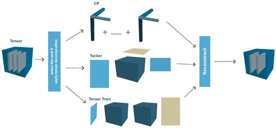
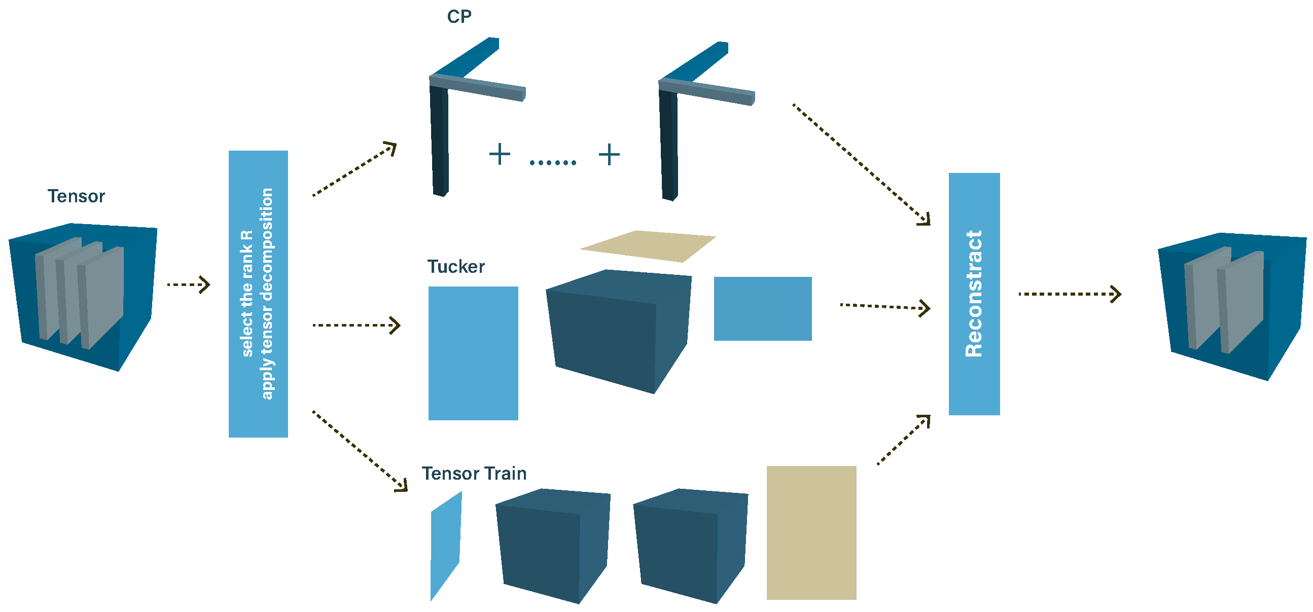
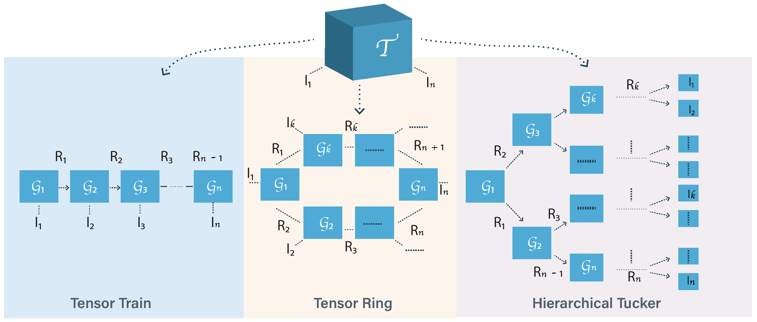
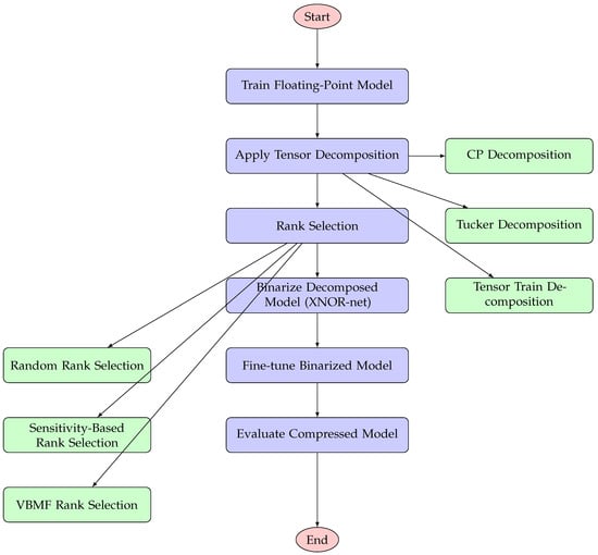
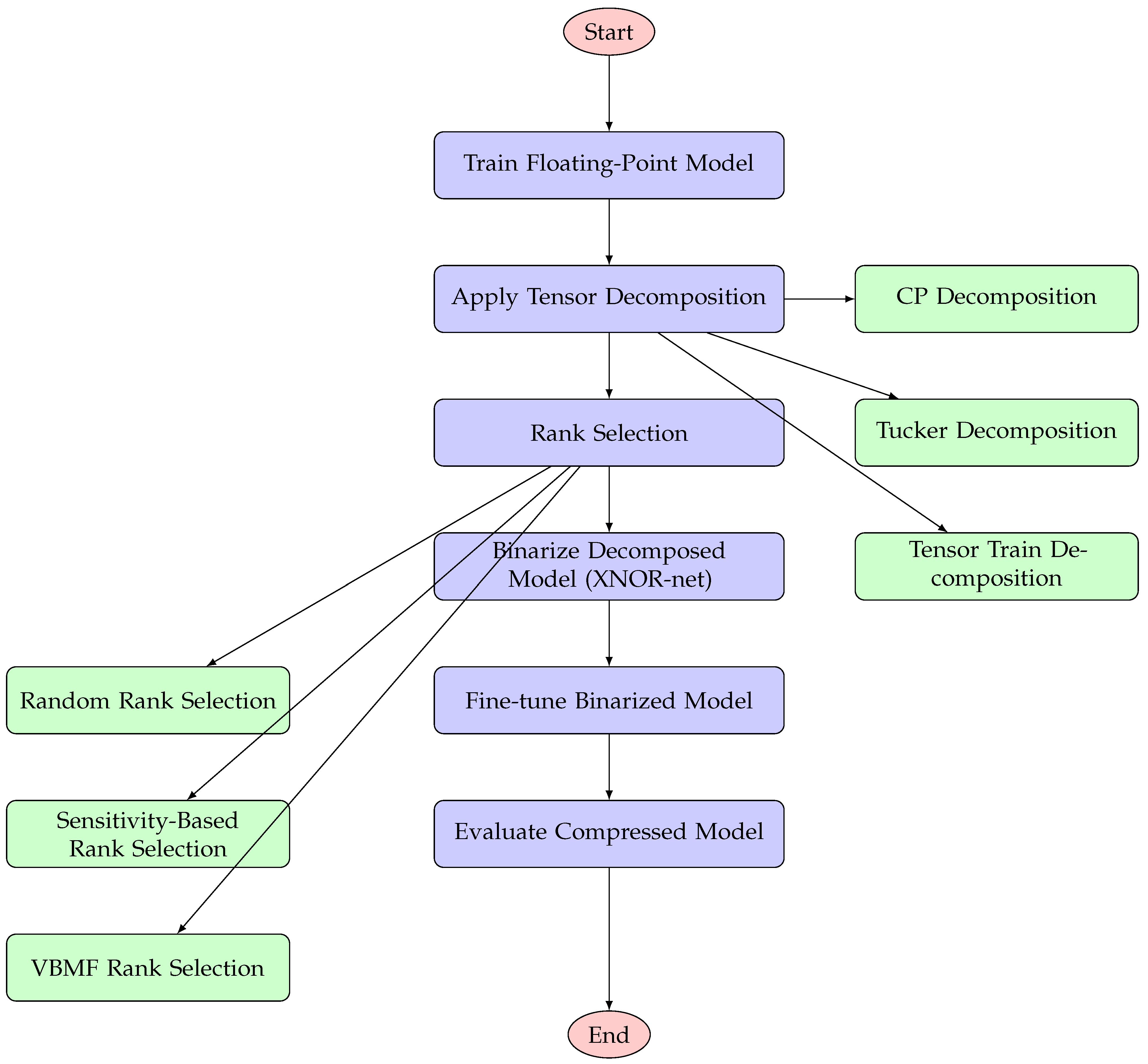
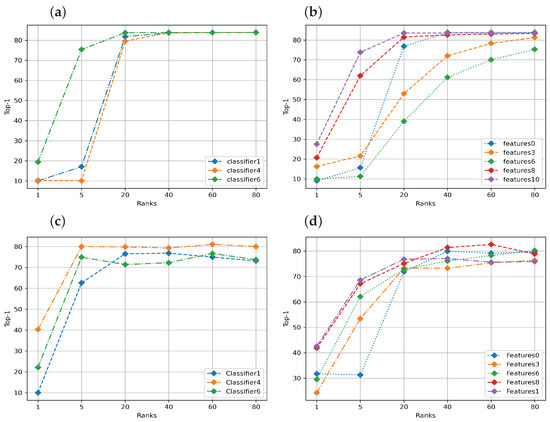
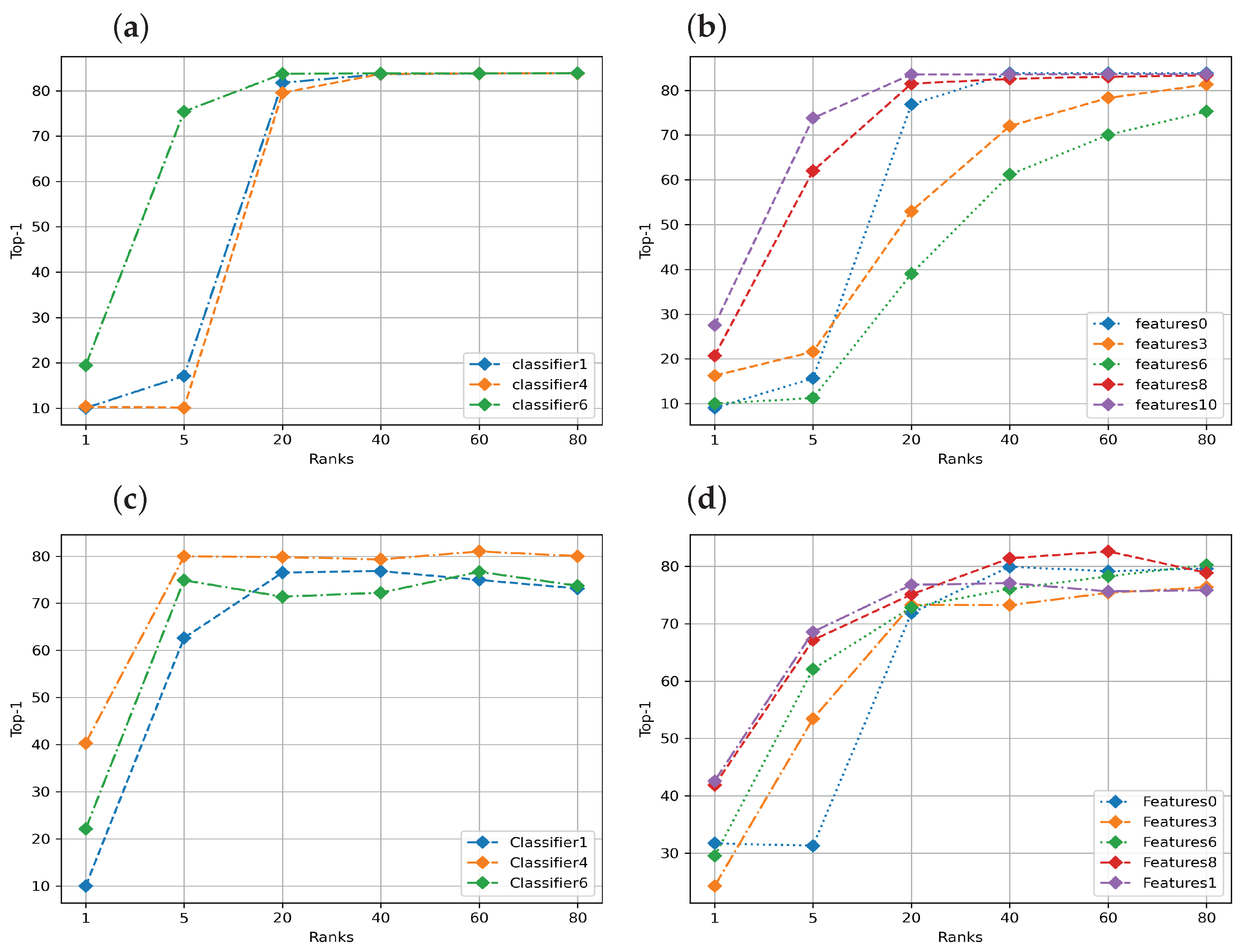
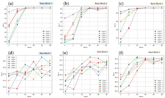
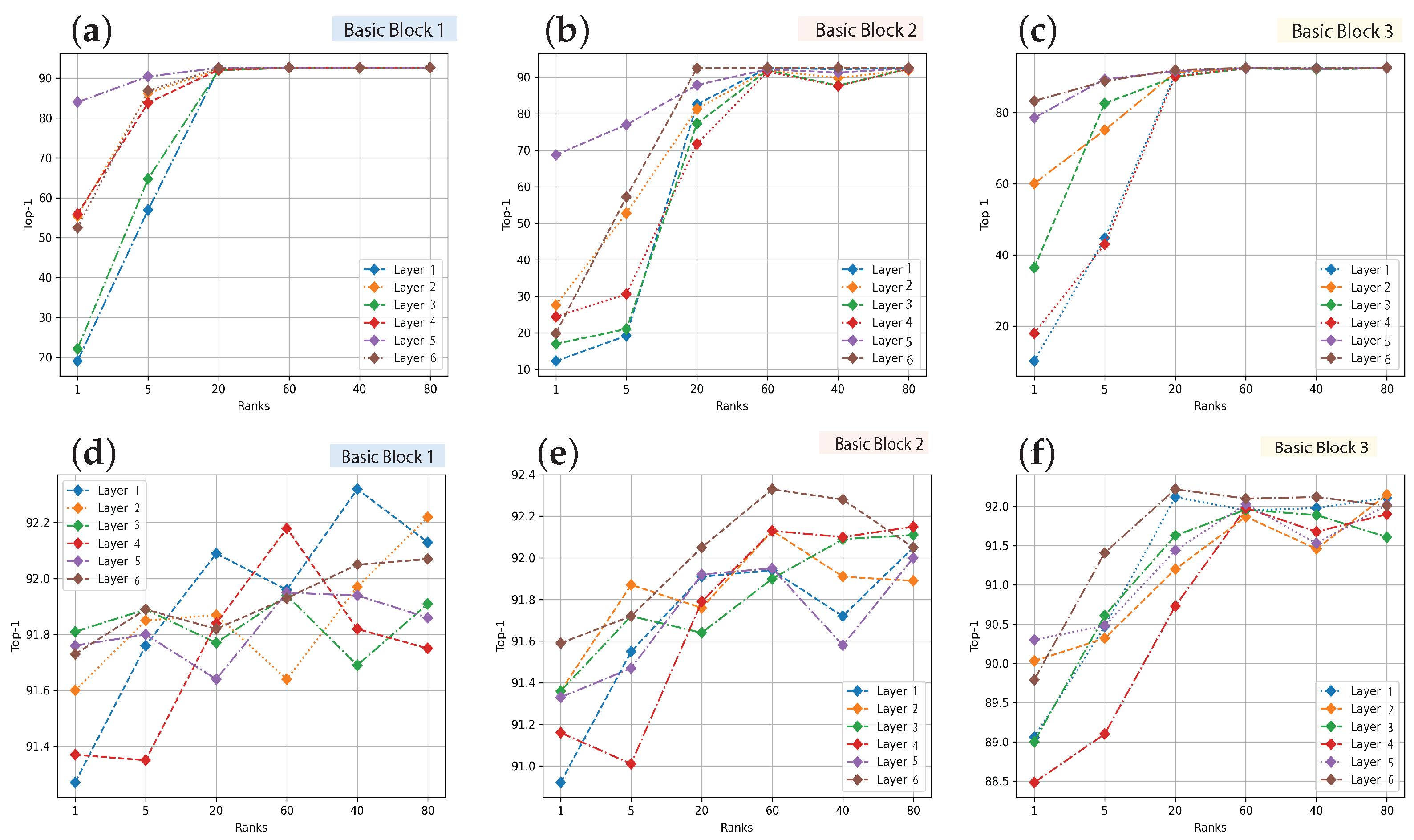
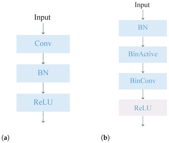
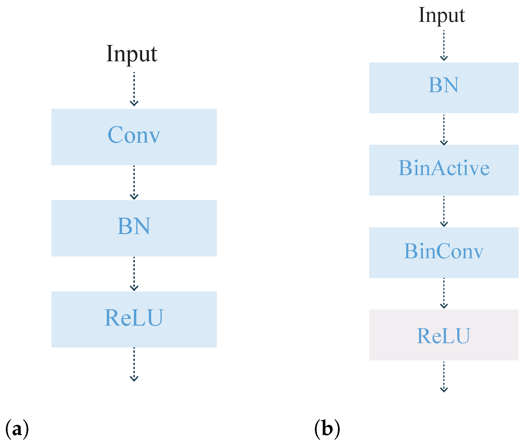
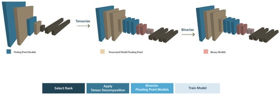
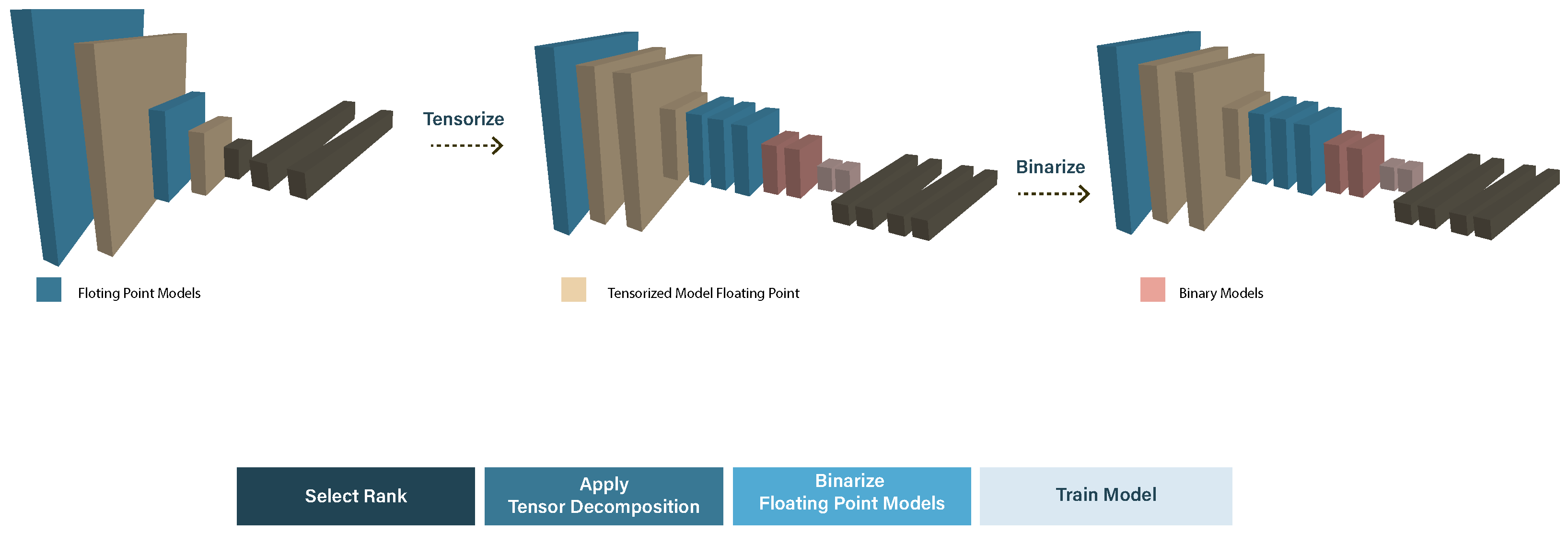
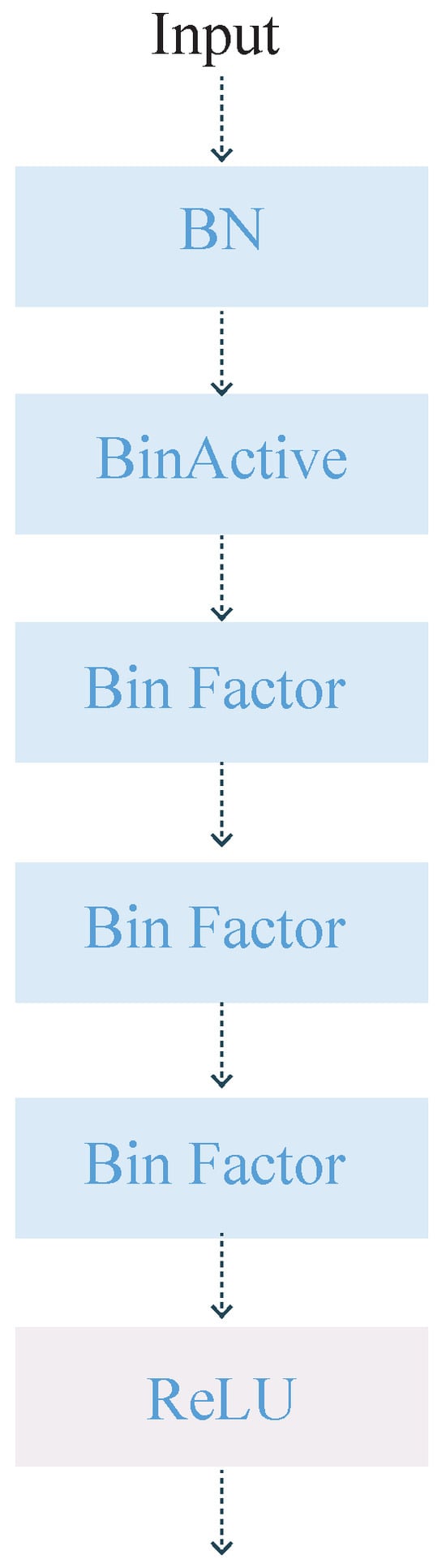
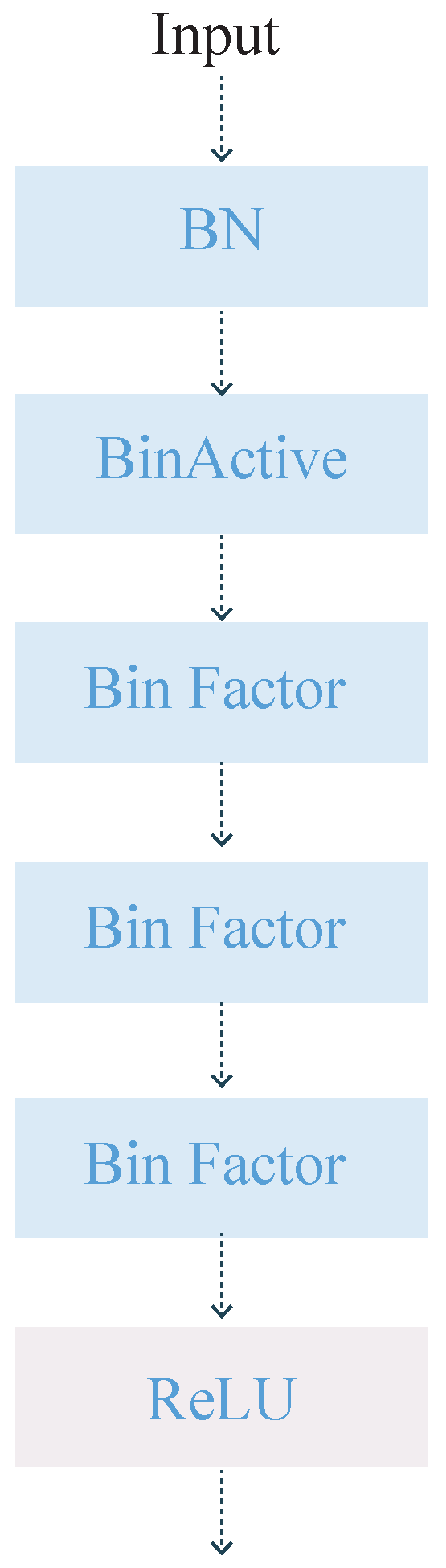
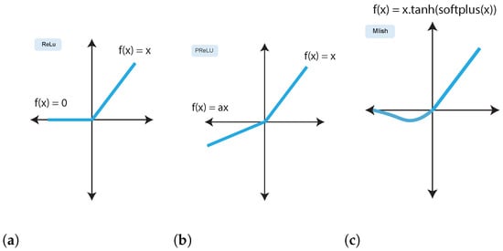
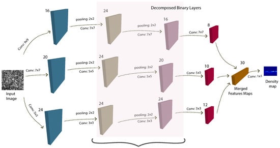
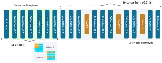

Disclaimer/Publisher’s Note: The statements, opinions and data contained in all publications are solely those of the individual author(s) and contributor(s) and not of MDPI and/or the editor(s). MDPI and/or the editor(s) disclaim responsibility for any injury to people or property resulting from any ideas, methods, instructions or products referred to in the content. |
© 2024 by the authors. Licensee MDPI, Basel, Switzerland. This article is an open access article distributed under the terms and conditions of the Creative Commons Attribution (CC BY) license (https://creativecommons.org/licenses/by/4.0/).