Article

A Data- and Model-Integrated Driven Method for Recommending the Maximum Safe Braking Deceleration Rates for Trucks on Horizontal Curves

School of Highway, Chang’an University, South 2nd Ring Road, Beilin District, Xi’an 710064, China
*
Authors to whom correspondence should be addressed.
Appl. Sci. 2024, 14(20), 9357; https://doi.org/10.3390/app14209357
Submission received: 24 July 2024 / Revised: 4 October 2024 / Accepted: 8 October 2024 / Published: 14 October 2024

Abstract

:
Truck skidding crashes on horizontal curves pose a significant road safety concern, with improper braking being the primary cause. A data- and model-integrated driven method is proposed to investigate the mechanism and recommend the maximum safe braking deceleration rates without skidding (abbreviated as MSBDRs) for trucks on horizontal curves. Firstly, a comprehensive road–vehicle interaction model was developed, considering dynamic changes in brake force distribution, vertical tire load, and longitudinal and side friction during braking. Secondly, leveraging the “HighD” data set and employing cluster analysis principles, parameter data were extracted using Python and Matlab. Finally, through parameterizing model inputs, the transient dynamic response of trucks was examined, the potential of truck skidding was predicted, and the MSBDRs were recommended. The results indicate the following. (1) There is little concern of truck skidding during car-following braking maneuvers; however, there is a high potential of truck skidding during emergency braking maneuvers. (2) The MSBDR is 4.5 m/s2 on a limit-minimum-radius horizontal curve; however, when combined with steep slopes, an overspeed exceeding 20%, and extremely wet road conditions, respectively, the MSBDRs decrease to 4 m/s2, 3 m/s2, and 2 m/s2. These results provide a theoretical foundation for braking strategies in autonomous vehicles.

1. Introduction

Road traffic crashes have become a worldwide concern. Horizontal curves, in particular, present a major challenge in traffic operations and safety due to their significantly higher crash rate [1]. According to statistics from the Federal Highway Administration in the United States, the average crash rate on horizontal curves is approximately three times higher than other road segments [2]. Previous studies and crash data have shown that truck skidding collisions are the primary type of crashes on horizontal curves [3,4,5]. Further analysis reveals that over 90% of truck crashes can be attributed to risky driving behaviors, with the improper braking maneuvers having the highest impact on truck skidding on horizontal curves [6,7].
Efforts have been made to prevent truck skidding on horizontal curves through roadway design, vehicle characteristics, and driver behavior since the 1940s [8,9,10,11,12]. Firstly, the road alignment directly influences the lateral stability of trucks. Current geometric design standards for horizontal curves are based on a mathematical model that represents vehicles as a point mass [13]. However, some studies have indicated that these standards often overestimate the lateral stability of vehicles, especially trucks [14,15,16]. The braking forces experienced during traversing horizontal curves can induce vehicle skidding when lateral acceleration is lower than suggested by the point mass model, with a greater impact on trucks [16]. Researchers have proposed using the bicycle model for road geometric design [17,18]. The bicycle model allows for the analysis of both force and moment balance in vehicles, as well as the examination of individual wheel skidding safety [19]. However, studies based on the bicycle model do not adequately consider the driver’s braking behavior. Since the 1960s, advancements in electronic computers and numerical calculation methods have enabled more complex multibody dynamics modeling and analysis [20,21].
Secondly, vehicle experts have developed safety devices such as the anti-lock brake system (ABS), which is designed to keep a vehicle steerable and stable during heavy braking moments by preventing wheel lock [22,23].
In addition to theoretical modeling research, some researchers have investigated the impact of braking maneuvers on vehicle skidding by analyzing statistics related to natural driving behavior [12,24,25,26,27]. These studies have yielded valuable findings, particularly in relation to characteristic parameters such as driver reaction time and braking deceleration. However, data-driven methods suffer from a black box effect and fail to explain the underlying mechanisms of the effect of the braking maneuvers on vehicle skidding. The issue of driving safety introduced by braking maneuvers is not only a challenge for traditional human driving behavior researchers but also an important focus for researchers in the field of autonomous and assisted driving [28,29,30]. These researchers primarily focus on analyzing braking strength, time-to-collision (TTC), emergency response time, and other characteristics of braking behavior to develop various collision avoidance control algorithms. However, these algorithms mainly prioritize longitudinal safety and lack consideration for lateral safety on horizontal curves during braking. As a result, there is a concern that while braking effectively reduces rear-end collision crashes, it may simultaneously increase the risk of more severe skidding collision crashes.
While significant efforts have been invested in transportation safety research, the issue of truck skidding collisions on horizontal curves remains inadequately addressed. This deficiency primarily stems from the absence of a comprehensive theoretical model that effectively accounts for the dynamic interaction between the road and the vehicle during pre-crash braking, along with the precise identification of critical model parameters. Consequently, accurately predicting the potential for truck skidding on horizontal curves during braking poses an ongoing challenge. Therefore, this paper proposes a data- and model-integrated driven approach to predict skidding potential and to recommend the maximum safe braking deceleration rates without skidding (abbreviated as MSBDRs) for trucks on horizontal curves. This study aims to address the limitations of human factors considerations in road design theories and effectively reduce truck skidding collision crashes on horizontal curves. Additionally, it can serve as a theoretical reference for braking strategy formulation for autonomous vehicles.
The rest of the paper is organized as follows. Section 2 introduces the existing studies on vehicle skidding from two research methods. In Section 3, the data- and model integrated-driven method is proposed. In Section 4, the maximum safe braking deceleration rates without skidding were recommended. Finally, discussions and conclusions are presented in Section 5 and Section 6.

2. Literature Review

2.1. Studies on Vehicle Skidding Based on the Model-Driven Method

The existing design policy for horizontal curves is based on a mathematical model that represents a vehicle as a mass point. According to this model, when a vehicle traverses a horizontal curve, it experiences centripetal acceleration that is balanced by superelevation and tire–pavement interface friction [13]. However, recent research has highlighted safety concerns associated with this model. MacAdam’s studies [31,32] have shown that when vehicles, especially trucks, traverse horizontal curves with longitudinal slopes, the application of braking and traction forces on a slope can result in dynamic variations in both vertical tire load and tire–pavement side friction. These variations may cause the vehicle to skid at lateral accelerations lower than predicted by the point mass model. To address these concerns, Kontaratos et al. [33] proposed an improved bicycle model that incorporates various factors such as slope, superelevation, front- and rear-wheel drive, and aerodynamic resistance. The bicycle model offers advantages over the point mass model as it allows for analysis of both force and torque balance of the vehicle. Furthermore, it enables the examination of individual axle skid [17]. However, the research lacks a comprehensive consideration of driver braking maneuvers. In Bonneson’s study [34], an enhanced bicycle model was presented, and slight braking scenarios for two-axle vehicles were analyzed. The findings indicated potential safety problems for roads with combined horizontal and vertical components. NCHRP Rep. No.774 proposed superelevation criteria for sharp horizontal curves on steep grades based on the findings of Torbic et al., using bicycle and multibody dynamics models [19]. Although the multibody model offers high accuracy and minimal errors, it incorporates the force analysis of various vehicle components, leading to complex influencing factors and solving procedures.
The impact of braking on vehicle skidding is related to the redistribution of braking force and lateral force [5,35,36]. Several studies have analyzed the relationship between tire braking force and lateral force during braking. Bergman [37] was the first to theoretically analyze the skidding characteristics during tire braking and designed an expression for the lateral force function, considering the braking force as a variable. Wong [38] proposed that, under specific conditions, the longitudinal and side friction relationship of tires follows a friction ellipse, with boundaries determined by the peak braking force (driving force) and peak lateral force. Ong and Fwa [39] simulated and analyzed vehicle skidding using a simulation model, and the study identified that factors such as water film thickness and driving speed significantly influence the peak friction coefficient of the vehicle. Peng et al. [40] used simulation models to calculate the peak friction under different operating conditions and analyzed three possible modes of skidding when vehicles travel on a horizontal curve.
The safety concerns arising from braking maneuvers pose significant challenges to researchers studying human driving behavior. They are also a critical focus of research for emerging autonomous driving and driver-assistance systems [5,10,30]. Automotive companies have proposed active braking collision avoidance algorithms that employ similar models. These algorithms utilize three key indicators—relative distance, relative velocity, and driving speed—to define the critical distance function for warning and active collision avoidance control. The brake control information is then computed by onboard computer systems and conveyed to the driver. This research primarily focuses on longitudinal collisions and pays insufficient attention to the lateral safety issues during braking on horizontal curves. Hence, a critical concern arises—while emergency braking effectively helps reduce rear-end collisions, it may give rise to more severe accidents involving skidding or rollover. Therefore, it is crucial to strategically plan safer and more efficient vehicle motion trajectories while maintaining lateral stability during braking [41].
The above studies show the following:
1. The point-mass model is not sufficient to assess the potential of truck skidding on horizontal curves.
2. The current design policy for horizontal curves, based on the point-mass model, fails to integrate road features, vehicle design, and driver behavior adequately, leading to inadequate safety measures for road users.
3. The present study focuses on predicting the potential of truck skidding on horizontal curves during different braking behaviors based on the bicycle model, but the bicycle model does not consider the dynamic changes in brake force distribution, vertical tire load, and longitudinal and side friction during braking. These aspects need to be further addressed to enhance the comprehensiveness of the models.
4. The existing automatic emergency braking and obstacle avoidance algorithms primarily focus on longitudinal collision avoidance, neglecting the lateral safety concerns associated with braking on horizontal curves.

2.2. Studies on Vehicle Skidding Based on the Data-Driven Method

Research efforts and crashes data showed that more than 90% of crashes were related to risky driving behaviors, the more common ones being speeding, improper braking, and steering [6]. Han et al. [42] proposed an LSTM + Transformer model to analyze risky driving behaviors by using a Transformer for spatial-temporal feature extraction and an LSTM for learning traffic flow patterns. Their empirical analysis on a Chinese freeway revealed that increased frequency, duration, and acceleration of risky braking behaviors heighten crash risks by affecting more vehicles. Kim et al. [43] integrated crash data experienced over a four-year period with three months of microscale driving behavioral data and detected a high propensity of drivers to decelerate at high rates (4 m/s2 or more) on the segments with high crash rates. In a study by Jun [44], driver behaviors (speeding, acceleration, and braking) and their correlation with crash risk were examined using data collected from an in-vehicle device equipped with GPS and on-board diagnostics. It was found that drivers involved in skidding crashes showed significant acceleration and deceleration activities. Similarly, Wang et al. [45] used a high-fidelity driving simulator to investigate the effects of situational urgency on drivers’ collision avoidance behaviors and observed that drivers quickly released the accelerator and applied maximum braking force with increasing situational urgency.
In addition, vehicle characteristics, especially the braking-system performance and tire properties have been shown to affect skidding [23,40]. An analysis of crashes in Florida revealed a reduction in skidding-related crashes by 6% and 8% for ABS-equipped passenger cars and trucks, respectively [23]. Modern vehicles, including both passenger cars and trucks, are typically equipped with an antilock braking system (ABS) to prevent wheel lock during hard braking or mitigate crash damage. The skid resistance of tires on pavement surfaces, influenced by tire type, inflation pressure, deformation, slip ratio, and slip angle, plays a significant role in vehicle skidding [39,40,46]. The data showed that the crash rate associated with skidding in wet weather is significantly higher than that in dry weather [39,40]. Xiao et al. [47] developed a fuzzy-logic model for predicting the risk of crashes that occur on wet pavements by using crash data and the corresponding traffic data collected from 123 sections of highway in Pennsylvania from 1984 to 1986.
While the existing studies have contributed to our understanding of the relationship between braking maneuvers and skidding, there are still several gaps that need to be addressed:
1. Braking maneuvers are closely related to the crash rate, but this relationship has not been quantified.
2. The data-driven method can’t explain the underlying mechanisms of the effect of braking maneuvers on vehicle skidding.
3. The data-driven method has its own characteristics. This method demonstrates significant advantages in exploring the microcharacteristics of driver braking behavior.
In summary, through the literature review, the following gaps are found:
  • The road geometric design based on the point mass model cannot reflect the truck attributes, nor does it account for the effect of braking maneuvers on truck skidding.
  • Researchers have proposed the utilization of the bicycle model to analyze the influence of braking on skid safety in flat curved road segments. However, it still remains a challenge of incorporating the dynamic effects induced by braking into the model without making it unsolvable.
  • A relatively comprehensive and uncomplicated model is needed to describe the road–vehicle interaction. When developing this model, it is crucial to consider dynamic changes in brake force distribution, vertical tire load, as well as longitudinal and lateral friction during braking.
  • The data-driven method has inherent limitations, often characterized by the elusive “black box” effect. While the method fails to provide a clear understanding of the underlying mechanisms behind braking maneuvers that result in truck skidding, it does contribute to exploring the microcharacteristics of driver braking behavior.

3. Methods

The main research methods of this paper can be summarized as follows:
1. A comprehensive road–vehicle interaction model was developed, considering dynamic changes in brake force distribution, vertical tire load, and longitudinal and side friction during braking.
2. Leveraging the “HighD” data set and employing cluster analysis principles, parameter data were extracted using Python 3.11 and Matlab R2020b.
3. Through parameterizing model inputs, the transient dynamic response of trucks was examined, the potential of truck skidding was predicted, and the MSBDRs were recommended.
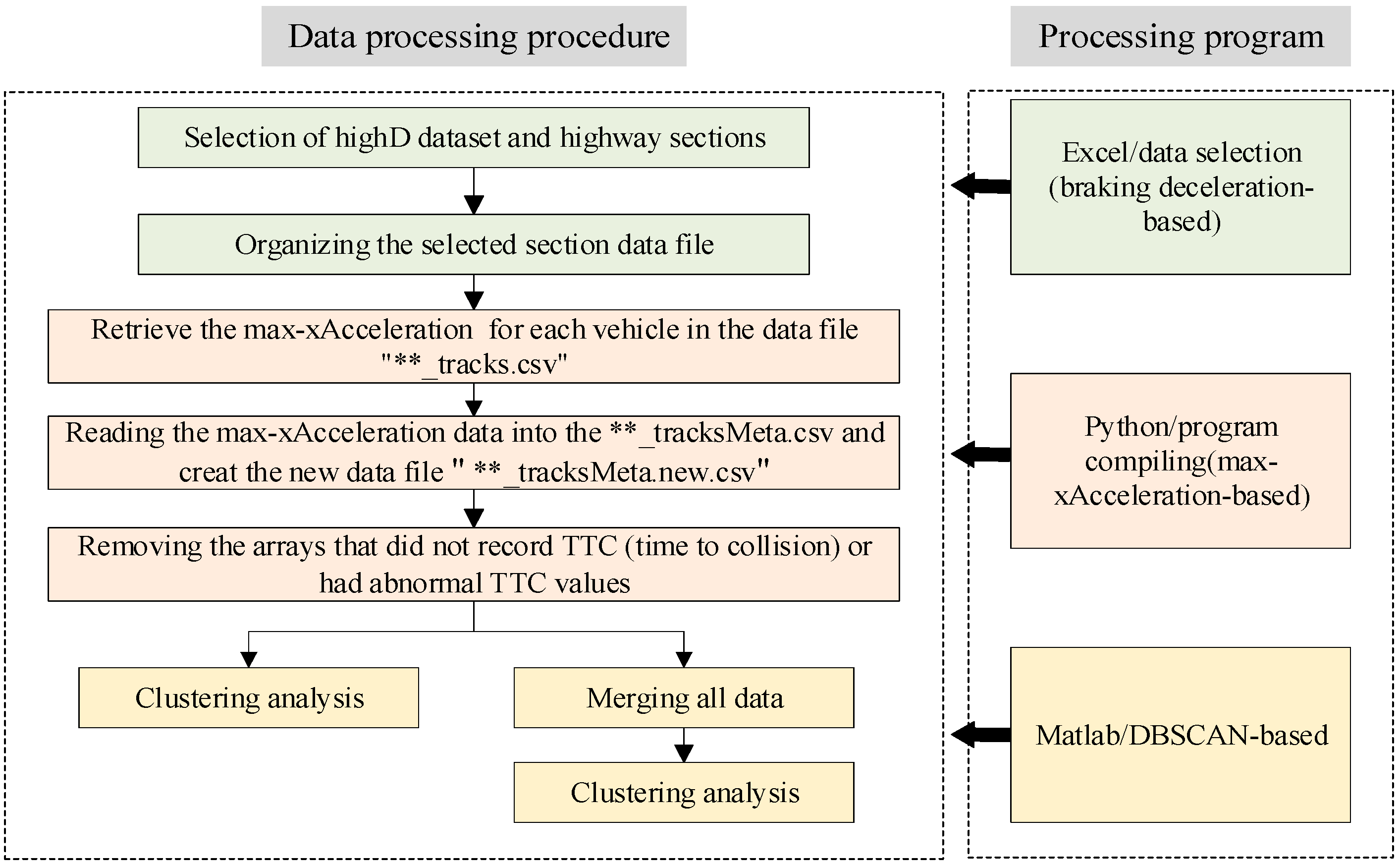
The specific process is shown in Figure 1.

3.1. Road–Vehicle Interaction Model

In this study, a road–vehicle interaction model was developed to analyze the vehicle dynamics response during braking on horizontal curves. The model is based on the bicycle model and takes into account the dynamic changes in brake force distribution, vertical tire load, and longitudinal and side friction during braking. Here is a brief introduction to the bicycle model.

3.1.1. Features and Limitations of the Bicycle Model

1.
Features of the bicycle model
The main criticism of the point-mass model is its failure to consider the per-axle force generation capabilities of a vehicle. This limitation prevents the model from accurately accounting for situations where one axle exceeds the friction limit while another remains below it, particularly on horizontal curves where braking affects the vertical tire load, as well as the longitudinal and side friction on each axle. To assess the impact of per-axle friction utilization, the bicycle model is employed, which idealizes the vehicle as a rigid beam and representing each axle as a single tire positioned at the vehicle’s midline [48]. It is utilized to evaluate the per-axle friction demand and ascertain whether the friction supply generated by the tire–pavement interface is sufficient for cornering during braking.
The bicycle model makes several basic assumptions [19] as follows: (1) the motion of the vehicle in the vertical direction (z-axis direction) is not considered, that is, the motion of the vehicle is assumed to be in a two-dimensional plane; (2) lateral load transfer is not taken into account; (3) the vehicle possesses right/left symmetry; (4) the suspension system of the vehicle is considered to be rigid and nonmoving throughout the curve; and (5) aerodynamics and rolling resistance of the tires are ignored.
2.
Model analysis
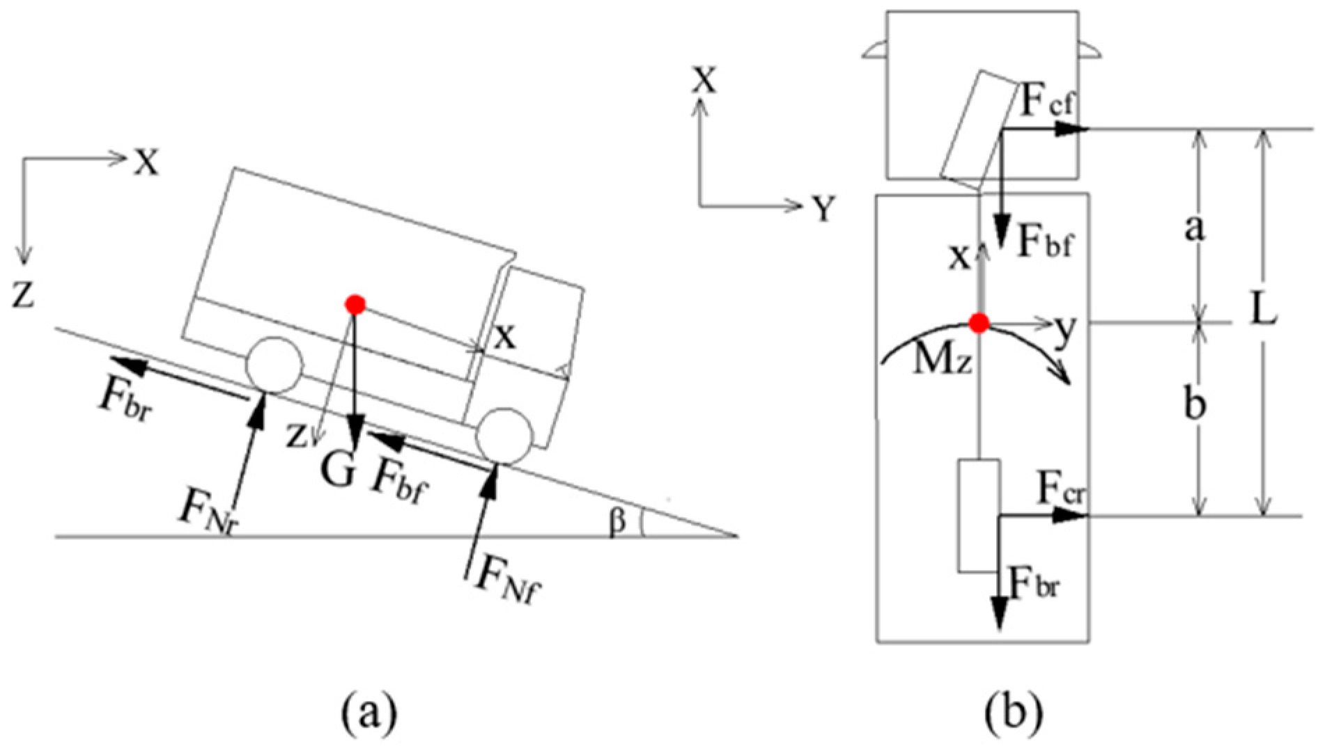
Lowercase x, y, and z are utilized to represent the coordinate system of the vehicle, while uppercase X, Y, and Z denote the coordinate system referenced to the Earth. The designations, as well as the forces acting along each axis, are illustrated in Figure 2. By employing small angle approximations, the following three governing equations can be derived separately for the local longitudinal (x-axis), lateral (y-axis), and vertical (z-axis) directions. The following Equations (1)–(19) refer to the research results of Torbic et al. [17].
Braking Equation:
Σ F x = F b f + F b r = m a x + m g i
Cornering Equation:
Σ F y = F c f + F c r = m v 2 / R m i h
Weight Balance Equation:
Σ F z = F N f + F N r = m g
where F b f is the braking force on the front axle, N; F b r is the braking force on the rear axle, N; F c f is the cornering force on the front axle, N; F c r is the cornering force on the rear axle, N; F N f is the vertical force on the front axle, N; F N r is the vertical force on the rear axle, N; i is the downgrade rate; i h is the superelevation rate; v is the velocity, m/s2; R is the circular curve radius, m; m is the mass, kg; and g is the gravitational acceleration, m/s2.
The vertical forces acting on each axis can be expressed as [11]
F N f = m g b / L + m a x + g i h g / L
F N r = m g a / L m a x + g i h g / L
Equations (4) and (5) demonstrate that the braking results in the weight transfer from the rear axle to the front axle. The magnitude of this weight transfer can be expressed as m a x + g i h g / L . It is worth noting that a higher deceleration rate corresponds to a greater amount of weight transfer.
The ratio of cornering forces between the front and rear axles can be determined by the following equation:
F c f / F c r = b / a
F c f / ( F c f + F c r ) = b / ( b + a ) = b / L
where a is the distance from the centroid to the front axle, m; b is the distance from the centroid to the rear axle, m; and h g is the CG height, m.
The cornering forces on each axle can be expressed as
F c f = b / L m v 2 / R m g i h
F c r = a / L m v 2 / R m g i h
The expressions for the side friction factors on each axle are
μ y f = F c f / F N f
μ y r = F c r / F N r
where μ y f is the side friction factor on the front axle and μ y r is the side friction factor on the rear axle.
Substituting Equations (4) and (8) into Equation (10), one obtains
μ y f = F c f / F N f = b / L m v 2 / R m g i h   m g b / L + m a x + g i h g / L
Substituting Equations (5) and (9) into Equation (11), one obtains
μ y r = F c r / F N r = a / L m v 2 / R m g i h m g a / L m a x + g i h g / L
Equations (12) and (13) depict the quasi-static friction demands for the front and rear axles for cornering during braking, respectively. These equations demonstrate the weight transfer from the rear axle to the front axle, resulting in an increased vertical force on the front axle. Consequently, a lower μ y f is sufficient to meet the cornering requirements. Conversely, the vertical force on the rear axle decreases, necessitating a higher μ y r to satisfy the cornering demands.
It is assumed here that F b f and F b r are known.
Then, the longitudinal friction factors on each axle can be determined by utilizing their basic definitions as follows:
μ x f = F b f / F N f
μ x r = F b r / F N r
where μ x f is the longitudinal friction factor on the front axle and μ x r is the longitudinal friction factor on the rear axle.
The side friction supply factors on each axle can be found based on the friction ellipse as follows:
μ y f , s u p p l y = μ y m a x , s u p p l y 1 μ x f / μ x m a x , s u p p l y 2
μ y r , s u p p l y = μ y m a x , s u p p l y 1 μ x r / μ x m a x , s u p p l y 2
where μ y f , s u p p l y is the side friction supply on front axle; μ y r , s u p p l y is the side friction supply on rear axle; and μ x m a x , s u p p l y is the maximum longitudinal friction supply. Note that when longitudinal friction factors ( μ x f ,   μ x r ) exceed the maximum longitudinal friction supply μ x m a x , s u p p l y ), it is assumed that the side friction supply factors ( μ y f , s u p p l y , μ y r , s u p p l y ) are zero.
The lateral friction margins are formulated as
μ y f , m a r g i n = μ y f , s u p p l y μ y f
μ y r , m a r g i n = μ y r , s u p p l y μ y r
where μ y f , m a r g i n is the lateral friction margin on the front axle and μ y r , m a r g i n is the lateral friction margin on the rear axle.
Equations (18) and (19) can be used to predict the skidding potential of the front and rear axles of the vehicle.
3.
Limitations of the bicycle model
Automotive theory indicates that, during the braking process, the actual braking force distribution among different axles of a vehicle is dynamically varying. The bicycle model does not consider the braking characteristics of trucks and lacks parameters related to the truck’s braking system, so it fails to accurately depict the dynamic changes in brake force distribution, vertical tire load, and longitudinal and side friction during braking. Consequently, it is unable to calculate the dynamic variations of F b f , F b r , and μ y f , m a r g i n , μ y r , m a r g i n . Furthermore, it does not provide accurate predictions of the skidding potential of the front and rear axles of trucks.

3.1.2. The Road–Vehicle Interaction Model

To address the limitations of the bicycle model, it is imperative to enhance its accuracy and effectiveness. By integrating the truck’s braking characteristics, the road–vehicle interaction model is development in this study.
1.
Truck’s braking characteristics
During braking, there exist three types of braking modes based on the sequential occurrence of wheel lock-up: front-wheel lock-up followed by skidding, rear-wheel lock-up followed by skidding, and simultaneous lock-up and skidding of both front and rear wheels [22,23]. Clearly, the simultaneous lock-up and skidding of both front and rear wheels demonstrates the most effective utilization of adhesion conditions.
The critical conditions for the occurrence of the braking modes are as follows:
  • φ < φ 0 : the position of the β-curve lies below the I-curve, implying that during braking, the front wheels consistently experience lock-up before the rear wheels.
  • φ > φ 0 : the position of the β-curve lies above the I-curve, signifying that during braking, the rear wheels consistently experience lock-up before the front wheels.
  • φ = φ 0 : in this scenario, during braking, both the front and rear wheels undergo simultaneous lock-up.
The β-curve represents the actual brake force distribution curve, the I-curve represents the ideal brake force distribution curve, and φ represents the maximum friction coefficient that can be generated between the tire and pavement; namely, φ 0 represents the synchronizing adhesion coefficient.
2.
Model development and analysis
Considering the brake force distribution under the three types of braking modes, the road–vehicle interaction model can be developed for vehicle dynamics response analysis.
(1)
Braking mode 1: φ < φ 0
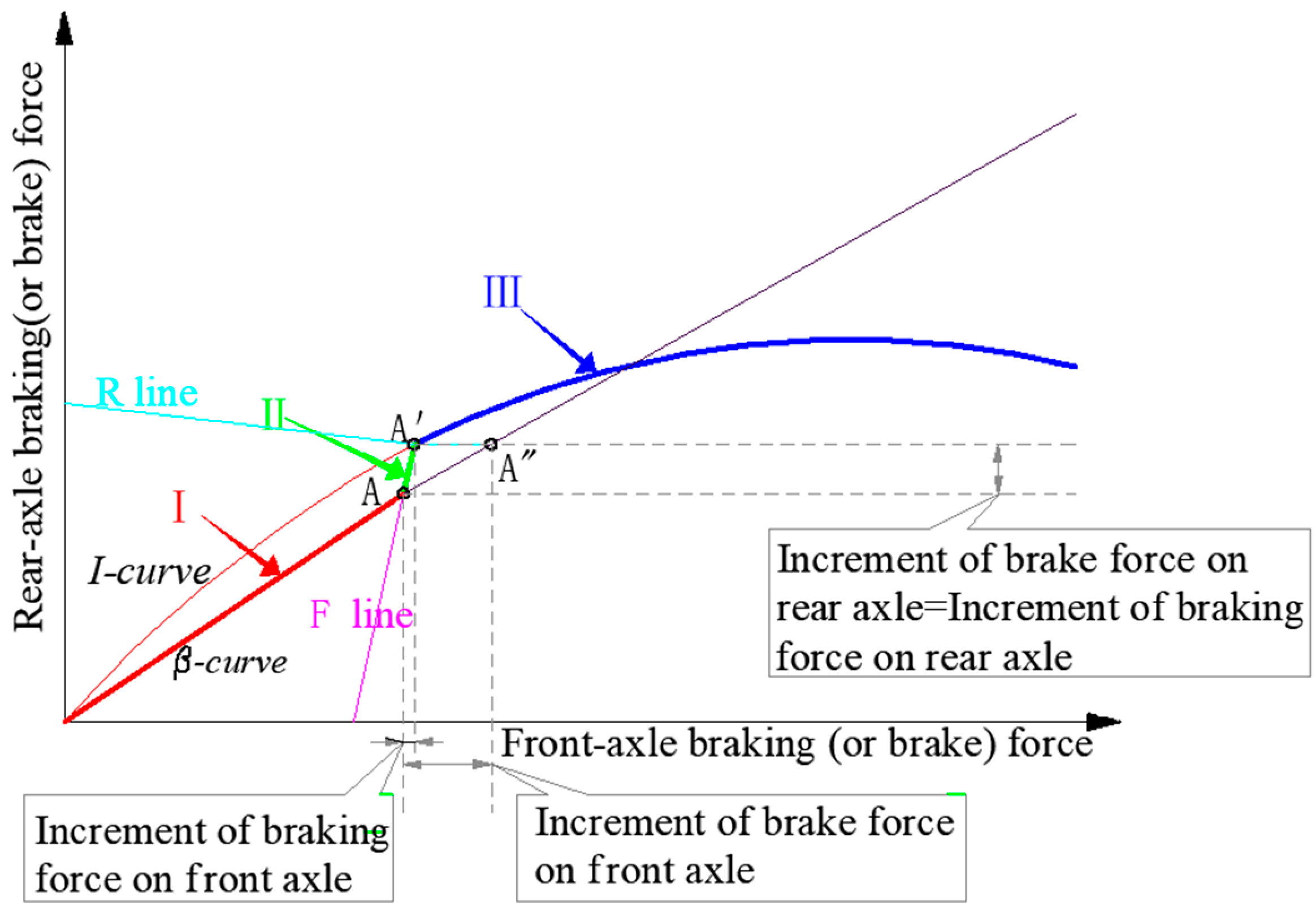
The dynamic change process of braking forces on front and rear axles can be divided into three stages during braking (marked in red, green, and blue, respectively), as shown in Figure 3.
Stage I. This stage is marked in red in Figure 3. Specifically, the braking forces on each axle increase along the β-curve. When the braking forces increase to point A, the front wheels lock up while the rear wheels do not, marking the end of stage I.
The braking deceleration rate of the truck at point A is recorded as a x 1 , and the ratio of the front-axle braking force to the rear-axle braking force at point A is given by
F b f / F b r = β ( 1 β )
F b f / F b r = μ x m a x , s u p p l y ( m g b / L + m a x 1 + g i h g / L ) m a x 1 + g i μ x m a x , s u p p l y ( m g b / L + m a x 1 + g i h g / L )
where β is the ratio of the front-axle braking force to total braking force and a x 1 is the braking deceleration rate of the vehicle at point A, m/s2.
Equations (20) and (21) can be combined to obtain
a x 1 / g = ( μ x m a x , s u p p l y b ) / ( β L μ x m a x , s u p p l y h g ) i
The expression of coefficient β is
β = ( φ 0 h g + b ) / L
Substituting Equation (23) into Equation (22), one obtains
a x 1 / g = ( μ x m a x , s u p p l y b ) / ( φ 0 h g + b μ x m a x , s u p p l y h g ) i
In stage I, a x < a x 1 , the braking forces on each axle can be expressed as
F b f = β F b = ( φ 0 h g + b )   ( m a x + m g i ) / L
F b r = 1 β F b = ( 1 ( φ 0 h g + b ) / L ) ( m a x + m g i )
Substituting these expressions into the given motion equations, Equations (14) and (15), and simplifying the results, the longitudinal friction factors on each axle become
μ x f = F b f / F N f = ( φ 0 h g + b ) / ( b / ( a x / g + i ) + h g )
μ x r = F b r / F N r = L φ 0 h g b / ( a / ( a x / g + i ) h g )
Substituting Equations (27) and (28) into Equations (16) and (17), respectively, the side friction supply factors on each axle become
μ y f , s u p p l y = μ y m a x , s u p p l y 1 ( φ 0 h g + b ( b / ( a x / g + i ) + h g )   μ x m a x , s u p p l y ) 2
μ y r , s u p p l y = μ y m a x , s u p p l y 1 L φ 0 h g b a / ( a x / g + i ) h g )   μ x m a x , s u p p l y 2
Thus, the front- and rear-axle lateral friction margins become
μ y f , m a r g i n = μ y m a x , s u p p l y 1 ( φ 0 h g + b ( b / ( a x / g + i ) + h g )   μ x m a x , s u p p l y ) 2 b V 2 / 127 R i h b + a x / g + i h g
μ y r , m a r g i n = μ y m a x , s u p p l y 1 L φ 0 h g b a / ( a x / g + i ) h g )   μ x m a x , s u p p l y 2 a V 2 / 127 R i h a a x / g + i h g
where a x / g is the normalized deceleration, g.
Based on the above analysis, we conclude that with the increase in braking deceleration rate, (1) the amount of weight transfer increases, (2) the front-axle side friction demand ( μ y f ) decreases, and the rear-axle friction demand ( μ y r ) increases, (3) the front- and rear-axle side friction supply factors ( μ y f , s u p p l y , μ y r , s u p p l y ) decrease, and (4) these result in a decrease in rear-axle side friction margin ( μ y r , m a r g i n ); i.e., the larger the braking deceleration rates, the lower is the potential of truck skidding,
Stage II. This stage is marked in green in Figure 3. The front wheels lock up while the rear wheels do not in this stage. Front- and rear-axle braking forces no longer increase along the β-curve, but along the F-line. Increasing the rear-axle braking force leads to an increase in the total braking force and, subsequently, an increase in truck deceleration. This results in a higher amount of weight transfer. During this stage, despite the front wheels locking up, the front-axle braking force continues to increase due to the increased front-axle vertical force. As the rear-axle braking force increases to point A′, the rear wheels lock up, marking the end of stage II.
The recorded braking deceleration rate of the truck at point A′ is denoted as a x 2 . Additionally, the front-axle and rear-axle braking forces at point A′ are specified as
F b f = μ x m a x , s u p p l y F N f ,   F b r = μ x m a x , s u p p l y F N r
F b f + F b r = μ x m a x , s u p p l y m g = m a x 2 + g i
Thus, the truck attains its maximum braking deceleration rate at point A′ when both the front and rear wheels lock up. This maximum deceleration rate is given by
a x 2 / g = μ x m a x , s u p p l y i
In stage II, a x 1 a x < a x 2 , the rear-axle braking force can be expressed as
F b r = m a x + g i μ x m a x , s u p p l y ( m g b / L + m a x + g i h g / L )
The rear-axle longitudinal friction factor becomes
μ x r = F b r / F N r = a x / g + i L μ x m a x , s u p p l y ( b + a x / g + i h g ) a a x / g + i h g
During this stage, the front-axle longitudinal friction factor ( μ x f ) has reached its maximum value ( μ x m a x , s u p p l y ), resulting in a zero front-axle side friction supply ( μ y f , s u p p l y ). Consequently, the front- and rear-axle lateral friction margins can be determined as
μ y f , m a r g i n = b V 2 / 127 R i h b + a x / g + i h g
μ y r , m a r g i n = μ y m a x , s u p p l y 1 a x / g + i L μ x m a x , s u p p l y ( b + a x / g + i h g ) ( a a x / g + i h g ) μ x m a x , s u p p l y 2 a V 2 / 127 R i h a a x / g + i h g
Stage III. This stage is marked in blue in Figure 3. As both the front and rear wheels lock up and the ABS system is activated, the front- and rear-axle braking forces vary along the I-curve. If the coefficient μ x m a x , s u p p l y remains constant, the braking force distribution curve also remains unchanged during this stage.
In stage III, the truck experiences a x = a x 2 , and the front- and rear-axle longitudinal friction factors ( μ x f , μ x r ) both reach their the maximum ( μ x m a x , s u p p l y ). As a result, the front- and rear-axle side friction supply factors become zero. Consequently, the front- and rear-axle lateral friction margins can be calculated as
μ y f , m a r g i n = b V 2 / 127 R i h b + a x / g + i h g
μ y r , m a r g i n = a V 2 / 127 R i h a a x / g + i h g
(2)
Braking mode 2: φ = φ 0
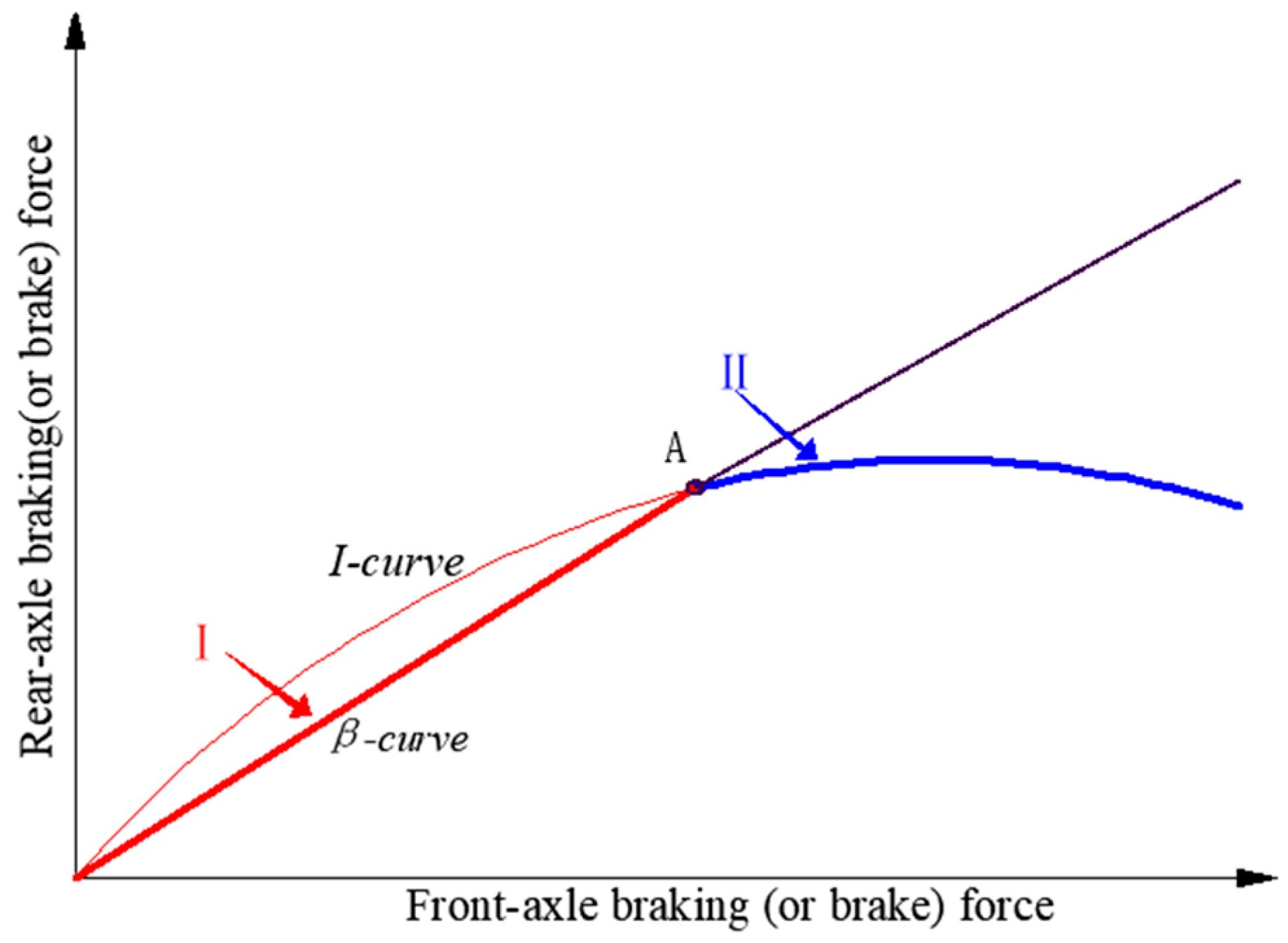
The dynamic change in braking forces on the front and rear axles can be divided into two stages during the braking process, which are marked in red and blue, respectively, in Figure 4.
Stage I. This stage is marked in red in Figure 4. Specifically, the braking forces on each axle increase along the β-curve. As the braking forces reach point A, the front and rear wheels lock up simultaneously, marking the end of stage I.
The braking deceleration rate of the truck at point A is recorded as a x 1 , the front- and rear-axle braking forces at point A are given by
F b f = μ x m a x , s u p p l y F N f ,   F b r = μ x m a x , s u p p l y F N r
F b f + F b r = μ x m a x , s u p p l y m g = m a x 1 + g i
The braking deceleration rate of the truck at point A can be expressed as
a x 1 / g = μ x m a x , s u p p l y i
In stage I, where a x < a x 1 , the calculation of the per-axle lateral friction margin remains the same as that in stage I of mode 1.
Stage II. This stage is marked in blue in Figure 4. The change in per-axle braking force is identical to that of stage III in mode 1.
In this stage, a x = a x 1 , the calculation of lateral friction margins remains the same as that in stage III of mode 1.
(3)
Braking mode 3: φ > φ 0
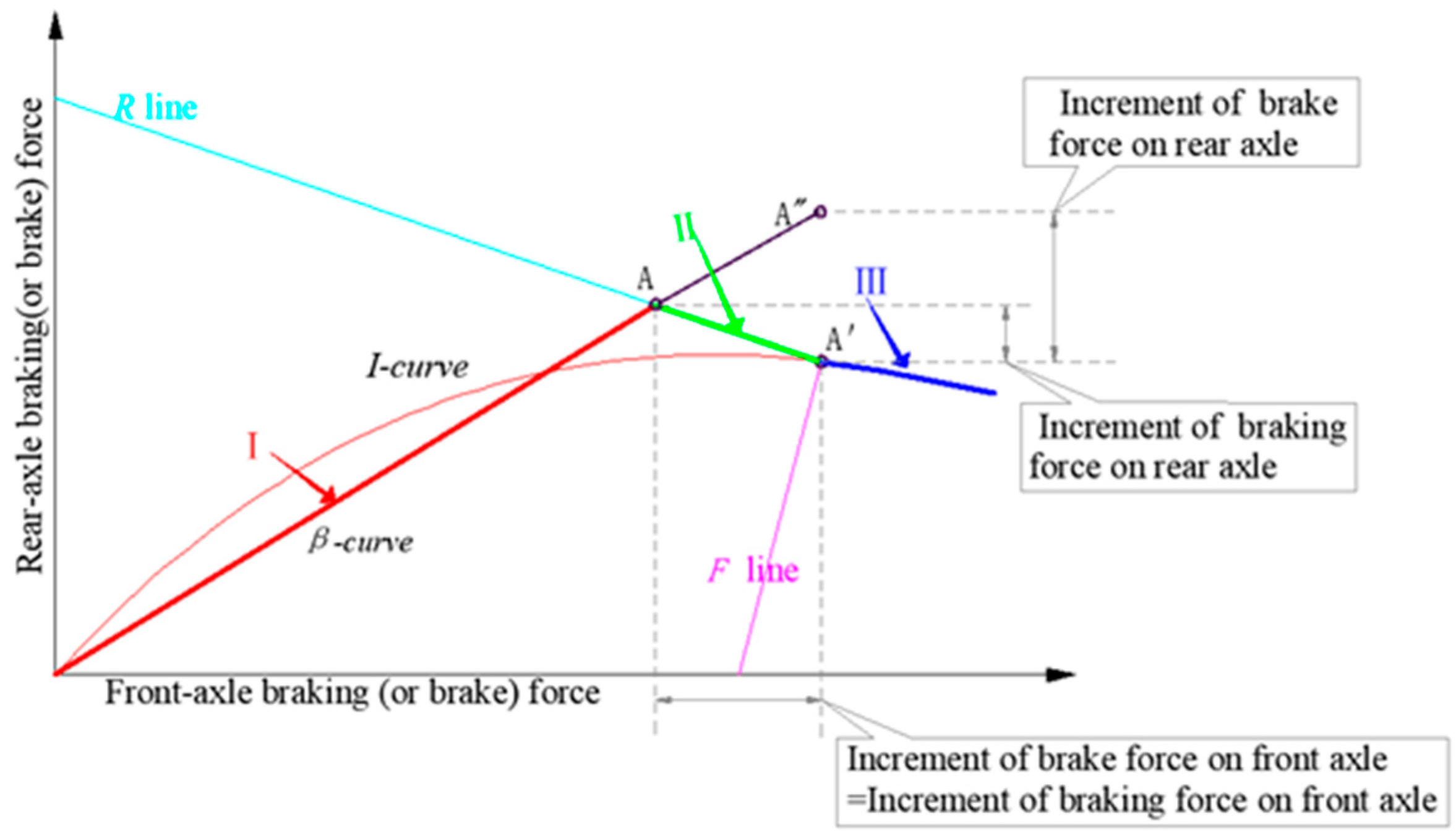
The dynamic change process of braking forces on front and rear axles can be divided into three stages during the braking (marked in red, green, and blue, respectively), as shown in Figure 5.
Stage I. This stage is marked in red in Figure 5. Specifically, the braking forces on each axle increase along the β-curve. The rear wheels lock up when the braking forces reach point A, while the front wheels do not, marking the end of stage I.
The braking deceleration rate of the truck at point A is recorded as a x 1 , and the ratio of front- and rear-axle braking forces at point A is given by
F b f / F b r = β 1 β
F b f / F b r = m a x 1 + g i μ x m a x , s u p p l y ( m g a / L m a x 1 + g i h g / L ) μ x m a x , s u p p l y ( m g a / L m a x 1 + g i h g / L )
Equations (45) and (46) can be combined to obtain
a x 1 / g = μ x m a x , s u p p l y a / ( L + μ x m a x , s u p p l y h g L β ) i
Substituting Equation (23) into Equation (38), one obtains
a x 1 / g = μ x m a x , s u p p l y a / ( L + μ x m a x , s u p p l y h g φ 0 h g b ) i
In stage I, where a x < a x 1 , the calculation of side friction margins remains the same as that in stage I of mode 1.
Stage II. This stage is marked in green in Figure 5. The rear wheels lock up and the front wheels do not. Front- and rear-axle braking forces no longer increase along the β-curve, but instead along the R-line. As the front-axle braking force increases, the total braking force and truck deceleration also increase, leading to an increase in the amount of weight transfer. Despite the rear wheels lock up, the rear-axle braking force continues to increase due to the increased rear-axle vertical force. When the braking forces reach point A′, the front wheels lock up, marking the end of stage II.
The braking deceleration rate of the truck at point A′ is recorded as a x 2 , and the calculation of a x 2 remains the same as that in stage II of mode 1.
In this stage, a x 1 a x < a x 2 , the front-axle braking force can be expressed as
F b f = m a x + g i μ x m a x , s u p p l y ( m g a / L m a x + g i h g / L )
The longitudinal friction factor on the front axle becomes
μ x f = F b f / F N f = a x / g + i L μ x m a x , s u p p l y ( a x / g + i h g ) b + a x / g + i h g
In stage II, the rear-axle longitudinal friction factor ( μ x r ) reaches its maximum ( μ x m a x , s u p p l y ); thus, the rear-axle side friction supply ( μ y r , s u p p l y ) is zero, and the front- and rear-axle lateral friction margins become
μ y f , m a r g i n = μ y m a x , s u p p l y 1 μ x f / μ x m a x , s u p p l y 2 b V 2 / 127 R i h b + a x / g + i h g
μ y r , m a r g i n = a V 2 / 127 R i h a a x / g + i h g
Stage III. This stage is in blue in Figure 5. The change of per-axle braking force remains the same as that in stage III of mode 1.
In this stage, where a x = a x 2 , the calculation of per-axle lateral friction margin remains the same as that in stage III of mode 1.

3.2. Model Parameter Identification

3.2.1. Identification of Vehicle Attributes and Road Properties Parameters

1.
Synchronous adhesion coefficient ( φ 0 )
When φ < φ 0 , the front axle locks up before the rear axle, resulting in a stable state. Therefore, in earlier vehicle designs, a larger synchronization adhesion coefficient (such as 0.8) was commonly used. However, an excessively large synchronization adhesion coefficient reduces the braking efficiency of the rear axle. This issue was only resolved after the invention of ABS. For vehicles equipped with ABS, φ 0 is generally between 0.4 and 0.5 [22]. In this study, the coefficient φ 0 is set at 0.4.
2.
Maximum longitudinal friction supply ( μ x m a x , s u p p l y )
The maximum longitudinal friction supply is associated with pavement performance, tire types, and the complex interaction of them. The study showed the maximum braking deceleration rates ( a x m a x ) available for passenger cars was about 0.8 g, that for buses was about 0.7 g, and that for trucks was about 0.6 g under good pavement conditions (e.g., dry asphalt concrete pavement) [49]. The relationship between the maximum braking deceleration rates and the maximum longitudinal friction factor is given by
μ x m a x , s u p p l y = a x m a x / g
Substituting a x m a x = 0.6 g into Equation (53), the maximum longitudinal friction supply is calculated to obtain μ x m a x , s u p p l y = 0.6.
The maximum longitudinal friction supply factors under different water film thickness conditions were proposed by Peng et al. [40] as follows:
(1)
Water film thickness: 0.5 mm, μ x m a x , s u p p l y = 0.5 ( μ y m a x , s u p p l y = 0.25 );
(2)
Water film thickness: 1 mm, μ x m a x , s u p p l y = 0.44 ( μ y m a x , s u p p l y = 0.22 );
(3)
Water film thickness: 2.5 mm, μ x m a x , s u p p l y = 0.34 ( μ y m a x , s u p p l y = 0.17 ).
To sum up, the maximum longitudinal friction supply is given by
μ x m a x , s u p p l y = 0.6 , W F T = 0 0.5 , W F T = 0.5 m m 0.44 , W F T = 1 m m 0.34 , W F T = 2.5 m m
3.
Maximum side friction supply ( μ y m a x , s u p p l y )
The maximum side and longitudinal friction supply factors were proposed by Lamm et al. [50] as follows:
μ x m a x , s u p p l y = 0.59 4.85 × 10 3 × V D S + 1.51 × 10 5 V D S 2
μ y m a x , s u p p l y = 0.27 2.19 × 10 3 × V D S + 5.79 × 10 6   V D S 2
where V D S is the design speed, m/s2.
In this study, the design speeds ( V D S ) are 120 km/h, 100 km/h, 80 km/h, and 60 km/h, respectively. One obtains μ y m a x ,   s u p p l y = 0.5 μ x m a x , s u p p l y .

3.2.2. Identification of Microcharacteristic Parameters of Driver Braking Behavior

1.
Data Collection
(1) Data set selection
To deeply explore the characteristics of driver braking behavior from a microscopic perspective, a large- and wide-scale data set of driver behavior is required. This not only requires advanced data acquisition devices but also accumulates data over time and space dimensions. Therefore, for this study, we have chosen the publicly available naturalistic driving behavior data set (HighD) published by the Institute for Automotive Engineering at RWTH Aachen University in Germany [51]. The reasons for selecting this database are threefold: (1) the university has long-standing research expertise and advantages in the fields of automotive engineering and autonomous driving; (2) the database can meet the precision and breadth requirements of this study; and (3) it has been widely utilized by many researchers in the study of driver behavior [25,26].
(2) Data set introduction
The HighD data set is a new collection of natural vehicle trajectories on German highways. It overcomes limitations of traditional traffic data collection methods by using a drone’s aerial perspective, which eliminates occlusions. The data set automatically extracts vehicle trajectories, including type, size, and maneuvers. It is also useful for tasks like analyzing traffic patterns and parameterizing driver models. The HighD data set includes a total of 60 highway sections. Each section data consists of four files, namely “**_highway.png”, “**_recordingMeta.csv”, “**_tracks.csv”, and “**_tracksMeta.csv”. For specific explanations and the coordinate system used for data collection, please refer to the official website.
(3) Data collection
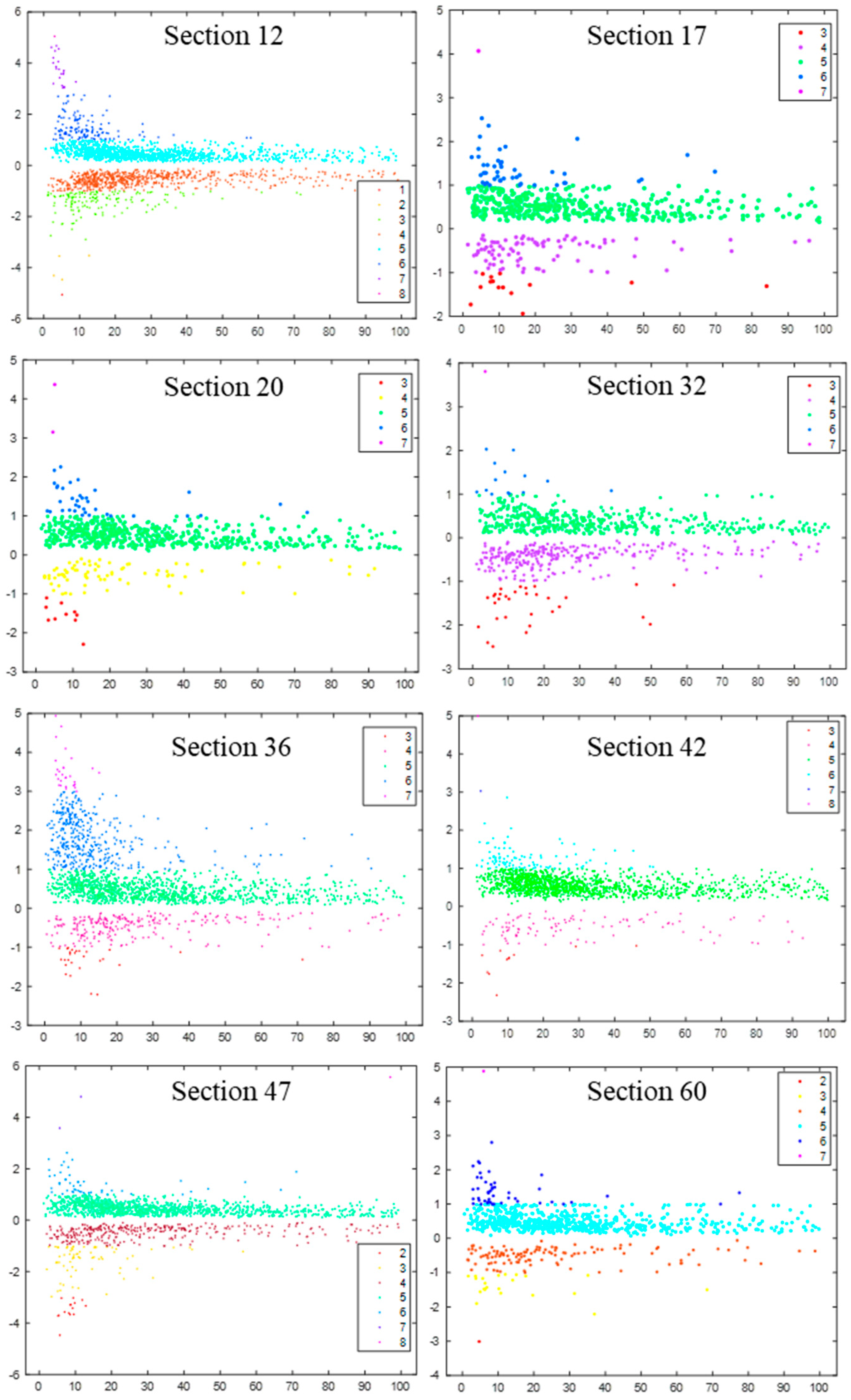
In this study, the data of eight highway sections (sections 12, 17, 20, 32, 36, 42, 47, 60) were selected due to their wider range of braking acceleration distribution. Each highway section is 420 m long.
2.
Data Reading and Processing
This step involves data reading and processing, as shown in Figure 6.
(1)
Utilizing Python programming, the data were compiled based on the data file “**_tracks.csv”. Within the recorded timeframe, the max-xAcceleration (maximum x Acceleration) for each vehicle (corresponding to each ID) was retrieved.
(2)
The filtering process is carried out to retain the arrays where the direction of max-xAcceleration is opposite to that of xvelocity.
(3)
The retrieved and filtered values of the max-xAcceleration are read into the data file “**_tracksMeta.csv”. A new data file “**_tracksMeta.new.csv” was created.
(4)
A further filtering process is conducted. The arrays that did not record TTC (time to collision) or had abnormal TTC values were removed in data file “**_tracksMeta.new.csv”.
(5)
Finally, the data file “**_tracksMeta.new.csv” from the eight highway sections were integrated into the data file “all_tracksMeta.csv”.
3.
Data Analysis and Parameter Identification.
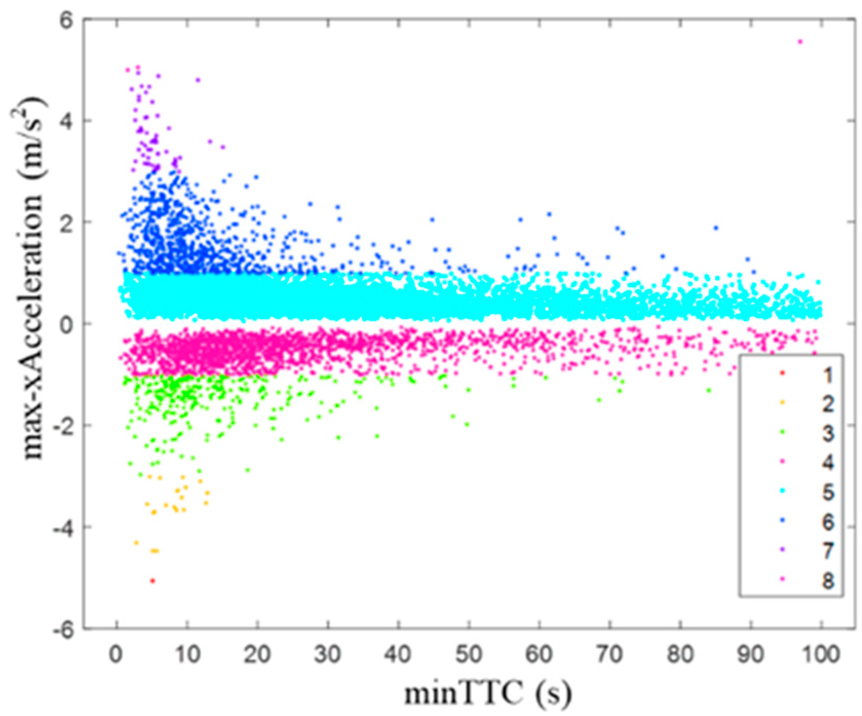
The TTC is used to quantify the urgency of driving conditions, with a smaller TTC indicating a more urgent situation. As a result, drivers tend to take more urgent braking maneuvers. To analyze the data, we conducted density-based clustering analysis using the Density-Based Spatial Clustering of Applications with Noise (DBSCAN) algorithm and implemented it in Matlab programming. The data set used for analysis includes the files “**_tracksMeta1.csv” and “all_tracksMeta.csv”. The x-axis and y-axis are the minTTC (minimum time to collision) and max-xAcceleration, respectively.
The data analysis results are shown in Figure 7 and Figure 8. Some preliminary conclusions can be drawn. (1) The data distribution of driver braking behavior is roughly the same in two driving directions on each highway section, (2) the max-xAcceleration values range from 0 to 5.5 m/s2, and (3) the data are clustered into eight clusters. The max-xAcceleration values ranges for clusters 1 to 8 are as follows: [4.5, 5.5], [3, 4.5), [1, 3), [0, 1), (−1, 0], (−3, −1], (−4.5, −3], [−5.5, −4.5].
Based on the clustering results, the ranges of deceleration are divided into four in accordance with the urgency of driving conditions, as presented in Table 1. According to previous literature [12,19,49], the deceleration values observed during car-following situations typically range below 1 m/s2, while deceleration based on stopping sight distance is generally below 3 m/s2. It is worth noting that when deceleration exceeds 3 m/s2, the driver can perceive a significant deceleration and feel discomfort. Furthermore, a deceleration greater than 4.5 m/s2 indicates an emergency brake situation. Based on these findings, we can classify driver braking behavior into four distinct types: car-following braking maneuvers, stopping-sight-distance braking maneuvers, significant braking maneuvers, and emergency braking maneuvers. These categories are summarized in Table 1.

4. Results

This study takes the FAW Jiefang J6M8×4 series truck as an example, which were selected because they accounted for a large proportion of trucks in China at present and because of their high crash rate and their operational characteristics [52,53]. For this type of truck, the first two axles are steering axles and they are the same in mechanical properties, and the last two axles are drive axles and they are the same in mechanical properties. Thus, the first and last two axles of this type of truck are regarded as the front and rear axles of the proposed model, respectively. This study performed calculations under different combinations of variables.
1.
Prediction of truck skidding potential and recommendations of the MSBDRs on horizontal curves with different curve radii. The parameter values in the model are shown in Table 2.
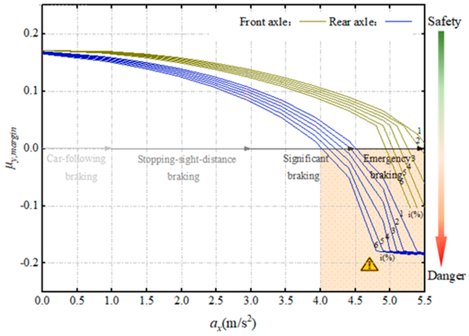
The results in Figure 9 show that:
  • During braking, there is a higher skidding potential of the rear axle compared to the front axle. In other words, the safety margin against skidding on front axle is met, but that of the rear axle is not necessarily met on horizontal curves during braking.
  • The curve radius has an effect on truck skidding. During braking, the smaller the radius of a horizontal curve, the higher the potential of skidding for trucks.
  • In addition to emergency braking maneuvers, the horizontal curves designed in accordance with the current road geometry design standards, even with the limit-minimum radius, provide an adequate safety margin against skidding for trucks.
  • During emergency braking maneuvers, the horizontal curves designed in accordance with the current road geometry design standards pose a high potential of trucks skidding. The higher the deceleration, the higher the potential of skidding for trucks.
  • Therefore, taking into consideration the objective of ensuring safety and mitigating skidding risks, the recommended MSBDR is 4.5 m/s2.
It is worth mentioning that, in the calculation, the radius of horizontal curves was determined as the limit-minimum radius for each design speed selected, in accordance with the design criteria. The results obtained here should assure that, if a truck can brake on a limit-minimum-radius curve without loss of control, then that same truck will be able to brake on larger-than-limit-minimum-radius curves without loss of control.
2.
Prediction of truck skidding potential and recommendations of the MSBDRs on horizontal curves with different slopes. The parameter values in the model are shown in Table 3.
The results in Figure 10 show that:
  • The downgrade has an effect on truck skidding.
  • During braking, a horizontal curve with steep slopes is more prone to inducing truck skidding compared to a single horizontal curve. The larger the downgrade rates, the higher the potential of truck skidding.
  • During significant and emergency braking maneuvers, trucks traveling on horizontal curves with steep slopes have a higher skidding potential.
  • Therefore, the recommended MSBDR is 4 m/s2 on horizontal curves with steep slopes.
3.
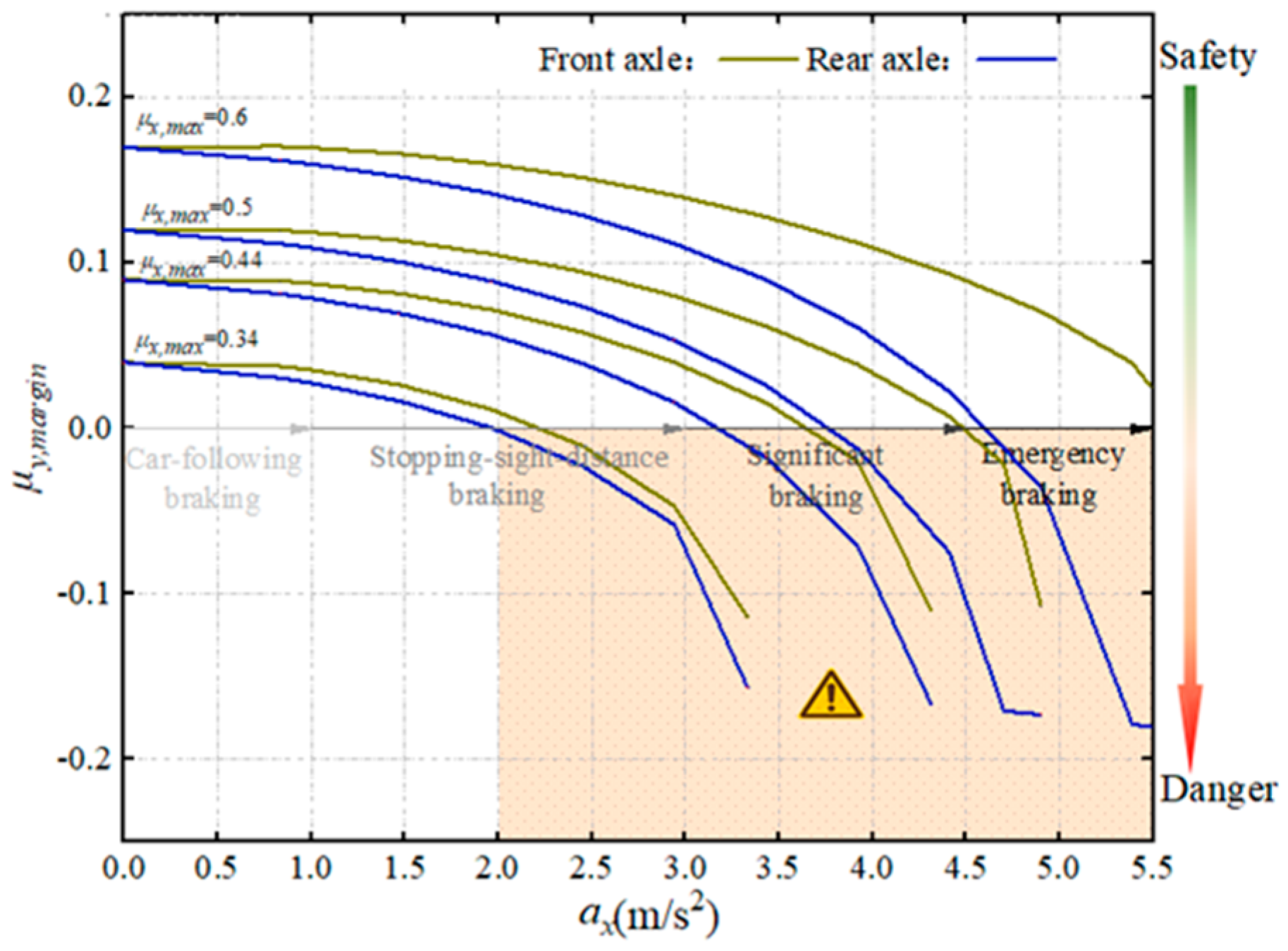
Prediction of truck skidding potential and recommendations of the MSBDRs on horizontal curves with different friction coefficients. The parameter values in the model are shown in Table 4.
The results in Figure 11 show that:
  • The friction coefficient has a significant effect on truck skidding.
  • The combination of braking and wet road conditions is worse for driving.
  • During braking, the lower the friction coefficient, the higher the potential of truck skidding.
  • On extremely wet roads (roads with a lower friction coefficient), even during stopping-sight-distance braking maneuvers, there is a higher potential of truck skidding.
  • Therefore, the recommended MSBDR is 2 m/s2 on an extremely wet horizontal curve.
4.
Prediction of truck skidding potential and recommendations of the MSBDRs on horizontal curves at different driving speeds. The parameter values in the model are shown in Table 5.
The results in Figure 12 show that:
  • Driving speed has a significant effect on truck skidding.
  • The combination of braking and speeding is worse for driving.
  • During braking, the more excessive the speeding, the higher the potential of truck skidding.
  • In cases of excessive speeding, during significant and emergency braking maneuvers, there is a higher potential of truck skidding.
  • Therefore, the recommended MSBDR is 2 m/s2 at a speed of 20% over the design speed on horizontal curves.
Summarizing the above findings, the following general conclusions can be drawn:
  • During braking, there is a higher skidding potential of the rear axle compared to the front axle.
  • The present study indicates that the effect of roadway alignment on the potential of truck skidding is very limited during braking.
  • Under any driving condition, there is little concern of truck skidding during car-following braking maneuvers; however, there is a high potential of truck skidding during emergency braking maneuvers.
  • Under wet road conditions and speeding conditions, there is the potential of truck skidding during sight-distance braking and significant braking.
  • In summary, the conditions most prone to causing truck skidding are the emergency braking, the combination of braking and wet road conditions, then the combination of braking and speeding.
  • Therefore, the recommended MSBDRs under different conditions are shown in Table 6.

5. Discussion

The scope of this contribution of this study was to introduce a new method to investigate the mechanism and degree to which braking affects the skidding potential and recommend the MSBDRs for trucks on horizontal curves.
It is found that in most cases, there is no concern of truck skidding while traveling at the design speed during braking on horizontal curves. Current design policy for horizontal curves is more forgiving for the driver, and the result supports the conclusions of Macadam and Harwood et al. [32]. But this study further pointed out that there is a higher potential of truck skidding during emergency braking on horizontal curves. The results are satisfactory compared with previous research results [48,52]. Due to the consideration of dynamic changes in brake force distribution, vertical tire load, and longitudinal and side friction during braking, it makes the prediction results more accurate. It is important that drivers and stakeholders understand the safety implications of risky braking maneuvers and the extent of the influence of risky braking maneuvers on vehicle skidding. Generally, it is known that drivers behave more safely when they are made aware of the risks or consequences of their driving styles (perceived behavior) [6,10,12].
This study provides a new perspective to investigate truck skidding on horizontal curves. This study fully integrates the advantages of model-driven and data-driven approaches. The integrated driven method can not only explain the underlying mechanisms of the effect of braking maneuvers on vehicle skidding, but also accurately quantify the impact of braking on skidding combined with big data analysis. It takes into account the dynamic changes in brake force distribution, vertical tire load, and longitudinal and side friction during braking. It considers driver behavior characteristics, vehicle attributes, and road properties in this study. It also makes the results widely applicable and more accurate.
This study will contribute to effectively reducing traffic crash injuries on horizontal curves. For example, this study found that the most critical driving scenarios arise during emergency braking, as well as when braking is combined with wet road conditions or speeding. As a result, drivers should pay particular attention to driving safety during braking in wet weather. Additionally, speed control plays a vital role for trucks on horizontal curves, especially those with smaller radii.
The findings of this research provide references and theoretical foundations for the formulation of autonomous driving braking strategies.

6. Conclusions

The objective of this study is to quantify the relationship between braking and the potential of truck skidding based on a data- and model integrated-driven method. Firstly, the road–vehicle interaction model was built considering the dynamic changes in brake force distribution, vertical tire load, and longitudinal and side friction during braking. Secondly, based on the “HighD” data set and employing the principles of cluster analysis, Python and Matlab were utilized to extract the data of driver behavior microcharacterization, vehicle attributes, and road properties. Thirdly, by parameterizing model inputs, the transient dynamic response of trucks was analyzed and the potential of truck skidding was predicted, and the MSBDRs were recommended.
The results show that:
1. The skidding potential differs significantly between truck axles during braking on horizontal curves, with the rear axle demonstrating higher susceptibility.
2. Under any driving condition, there is little concern of truck skidding during car-following braking maneuvers; however, there is a high potential of truck skidding during emergency braking maneuvers.
3. The MSBDR is 4.5 m/s2 on a limit-minimum-radius horizontal curve; however, when combined with steep slopes, an overspeed exceeding 20%, and extremely wet road conditions, respectively, the MSBDRs decrease to 4 m/s2, 3 m/s2,and 2 m/s2,
Although there are important discoveries revealed by this study, there are also limitations. Some aspects were neglected, such as the influence of difference of per-wheel force on research results.
The data for this study were primarily obtained from the HighD data set in Germany. Further research could focus on the variations in braking characteristics among drivers from different countries to determine if these should be considered in models.

Author Contributions

T.X.: methodology, investigation, software, formal analysis, data curation, writing—original draft, writing—review and editing. J.X.: conceptualization, validation, supervision, writing—review and editing. All authors have read and agreed to the published version of the manuscript.

Funding

This research was funded by the Fundamental Research Funds for the Central Universities, CHD, grant number 300102214110.

Institutional Review Board Statement

Not applicable.

Informed Consent Statement

Not applicable.

Data Availability Statement

The original contributions presented in the study are included in the article, further inquiries can be directed to the corresponding authors.

Conflicts of Interest

The authors declare no conflicts of interest.

Appendix A

Table A1. Key terms and their definitions.
Key TermsSymbolDefinitions
Side friction supply μ y , s u p p l y Friction available between the pavement surface and vehicle tires to prevent skidding in the radial (side) direction, also referred to as the coefficient of side friction.
Maximum side friction supply μ y m a x , s u p p l y The maximum side friction supply is utilized when a vehicle is at the point of impending skid in the radial (side) direction.
Longitudinal friction supply μ x , s u p p l y Friction available between the pavement surface and vehicle tires to prevent skidding in the tangential (longitudinal) direction, also referred to as the coefficient of longitudinal friction.
Maximum longitudinal friction supply μ x m a x , s u p p l y The maximum longitudinal friction supply is utilized when a vehicle is at the point of impending skid in the tangential (longitudinal) direction.
Side friction factor μ y The unbalanced portion of lateral acceleration or the portion of lateral acceleration that is not balanced by superelevation. The side friction factor represents the vehicle’s need for side friction, also called the side friction demand.
Lateral friction margin μ y f , m a r g i n The difference between the available tire–pavement friction and the friction demand of the vehicle as it tracks the curve (i.e., side friction supply ( μ y , s u p p l y )—side friction factor ( μ y )). This friction margin represents the additional lateral acceleration that a vehicle could undergo without skidding. A positive margin indicates that a vehicle can undergo additional lateral acceleration without skidding, while a negative margin indicates that the vehicle tires will skid given the level of friction supplied between the tire and pavement for the condition in question.
Ideal braking force distribution curveI-curveA relation curve of braking forces on front and rear axles when front and rear axles are locked at the same time. The further the point on the curve being from the origin, the larger is the maximum longitudinal friction supply.
Actual braking force distribution curveβ-curveIn fact, the braking forces on front and rear axles adopt linear distribution. The variation curve of braking forces on front and rear axles is represented as a straight line passing through the origin on the distribution graph.
Synchronous adhesion coefficient φ 0 The friction coefficient at the intersection of I-curve and β-curve of the vehicle is called the synchronous adhesion coefficient.
F line groupF-lineA series of braking force distribution curves, which represent the variation relationship between the front- and rear-axle braking forces in the case of front-axle lock-up.
R line groupR-lineA series of braking force distribution curves, which represent the variation relationship between the front- and rear-axle braking forces in the case of rear-axle lock-up.
Braking force The braking force of the ground acting on the wheel, i.e., the friction between the pavement surface and the tires, whose direction is opposite to the driving direction of the vehicle.
Brake force The braking force of the brake acting on the wheel, which depends on the brake torque and wheel radius.

References

  1. FHWA. Horizontal Curve Safety. 2024. Available online: https://safety.fhwa.dot.gov/roadway_dept/countermeasures/horicurves/ (accessed on 20 July 2024).
  2. FHWA. Roadway Departure Safety. 2024. Available online: https://safety.fhwa.dot.gov/roadway_dept/ (accessed on 20 July 2024).
  3. NHTSA. Traffic Safety Facts 2012: A Compilation of Motor Vehicle Crash Data from the Fatality Analysis Reporting System and the General Estimates System; NHTSA: Washington, DC, USA, 2013.
  4. Furtado, G.; Easa, S.; Abd, E. Vehicle Stability on Combined Horizontal and Vertical Alignments. In Proceedings of the Annual Conference of the Canadian Society of Civil Engineers, Montreal, QC, Canada, 5–8 June 2002. [Google Scholar]
  5. Choudhari, T.; Maji, A. Modeling driver’s braking and steering behavior along horizontal curves of two-lane rural highways for ADAS applications. Traffic Inj. Prev. 2022, 23, 404–409. [Google Scholar] [CrossRef] [PubMed]
  6. Petridou, E.; Moustaki, M. Human factors in the causation of road traffic crashes. Eur. J. Epidemiol. 2000, 16, 819–826. [Google Scholar] [CrossRef] [PubMed]
  7. Gaspar, J.; Brown, T.; Schwarz, C.; Chrysler, S.; Gunaratne, P. Driver Behavior in Forward Collision and Lane Departure Scenarios. In SAE Technical Paper Series; SAE: Warrendale, PA, USA, 2016. [Google Scholar]
  8. Barnett, J.; Haile, E.R.; Moyer, R.A. Safe Side Friction Factors and Superelevation Design. In Highway Research Board Proceedings; Highway Research Board: Washington, DC, USA, 1937; Volume 16. [Google Scholar]
  9. Aram, A. Effective Safety Factors on Horizontal Curves of Two-lane Highways. J. Appl. Sci. 2010, 10, 2814–2822. [Google Scholar] [CrossRef]
  10. Ali, Y.; Haque, M.M.; Zheng, Z.; Afghari, A.P. A Bayesian correlated grouped random parameters duration model with heterogeneity in the means for understanding braking behaviour in a connected environment. Anal. Methods Accid. Res. 2022, 35, 100221. [Google Scholar] [CrossRef]
  11. Sayers, M.W.; Mousseau, C.W.; Gillespie, T.D. Using simulation to learn about vehicle dynamics. Int. J. Veh. Des. 2002, 29, 112–127. [Google Scholar] [CrossRef]
  12. Li, S.; Li, P.; Yao, Y.; Han, X.; Xu, Y.; Chen, L. Analysis of drivers’ deceleration behavior based on naturalistic driving data. Traffic Inj. Prev. 2020, 21, 42–47. [Google Scholar] [CrossRef]
  13. AASHTO. A Policy on Geometric Design of Highways and Streets; American Association of State Highway and Transportation Officials: Washington, DC, USA, 2018. [Google Scholar]
  14. Harwood, D.W.; Mason, J.M.; Glauz, W.D.; Kulakowski, B.T.; Fitzpatrick, K. Truck Characteristics for Use in Highway Design and Operation. Volume II: Appendixes. Final Report; Data collection; Turner-Fairbank Highway Research Center: McLean, VA, USA, 1990. [Google Scholar]
  15. Harwood, D.W.; Mason, J.M., Jr. Horizontal curve design for passenger cars and trucks. Transp. Res. Rec. 1994, 1445, 22–33. [Google Scholar]
  16. Harwood, D.W.; Torbic, D.J.; Richard, K.R.; Glauz, W.D.; Elefteriadou, L. Review of Truck Characteristics as Factors in Roadway Design; Nchrp Report; Transportation Research Board: Washington, DC, USA, 2003. [Google Scholar]
  17. Torbic, D.J.; Donnell, E.T.; Brennan, S.N.; Brown, A.; O’Laughlin, M.K.; Bauer, K.M. Superelevation Design for Sharp Horizontal Curves on Steep Grades. Transp. Res. Rec. J. Transp. Res. Board 2014, 2436, 81–91. [Google Scholar] [CrossRef]
  18. Chang, T.H. Effect of Vehicles’ Suspension on Highway Horizontal Curve Design. J. Transp. Eng. 2001, 127, 89–91. [Google Scholar] [CrossRef]
  19. Torbic, D.J.; O’Laughlin, M.K.; Harwood, D.W.; Bauer, K.M.; Bokenkroger, C.D.; Lucas, L.M.; Ronchetto, J.R.; Brennan, S.; Donnell, E.; Brown, A. Superelevation Criteria for Sharp Horizontal Curves on Steep Grades; Transportation Research Board: Washington, DC, USA, 2014. [Google Scholar]
  20. Brandt, A.; Jacobson, B.; Sebben, S. High speed driving stability of road vehicles under crosswinds: An aerodynamic and vehicle dynamic parametric sensitivity analysis. Veh. Syst. Dyn. 2022, 60, 2334–2357. [Google Scholar] [CrossRef]
  21. Tang, G.; Ren, C.; Li, C. A Determination Method of Safety Driving Speeds on Different Radii Based on Trucksim. J. Highw. Transp. Res. Dev. 2016, 33, 134–139. [Google Scholar]
  22. Aly, A.A.; Zeidan, E.-S.; Hamed, A.; Salem, F. An Antilock-Braking Systems (ABS) Control: A Technical Review. Intell. Control. Autom. 2011, 2, 10. [Google Scholar] [CrossRef]
  23. Allen, K. The Effectiveness of ABS in Heavy Truck Tractors and Trailers; Department of Transportation: Washington, DC, USA, 2010.
  24. Bin, W.U.; Xichan, Z.H.U.; Jianping, S. Driver Emergency Braking Behavior Based on Naturalistic Driving Data. J. Tongji Univ. 2018, 46, 1514–1519. [Google Scholar]
  25. Hu, Y.; Li, Y.; Huang, H.; Lee, J.; Yuan, C.; Zou, G. A high-resolution trajectory data driven method for real-time evaluation of traffic safety. Accid. Anal. Prev. 2022, 165, 106503. [Google Scholar] [CrossRef]
  26. Kurtc, V. Studying car-following dynamics on the basis of the HighD dataset. Transp. Res. Rec. 2020, 2674, 813–822. [Google Scholar] [CrossRef]
  27. Olleja, P.; Bärgman, J.; Lubbe, N. Can non-crash naturalistic driving data be an alternative to crash data for use in virtual assessment of the safety performance of automated emergency braking systems? J. Saf. Res. 2022, 83, 139–151. [Google Scholar] [CrossRef]
  28. Hattori, Y.; Ono, E.; Hosoe, S. Optimum vehicle trajectory control for obstacle avoidance problem. IEEE/ASME Trans. Mechatron. 2006, 11, 507–512. [Google Scholar] [CrossRef]
  29. Abdel-Aty, M.; Cai, Q.; Wu, Y.; Zheng, O. Evaluation of automated emergency braking system’s avoidance of pedestrian crashes at intersections under occluded conditions within a virtual simulator. Accid. Anal. Prev. 2022, 176, 106797. [Google Scholar] [CrossRef]
  30. Wang, X.; Zhou, Y.; Cafiso, S.D. Automatic Emergency Braking System for Trucks for Two-Wheeler Longitudinal Collision Avoidance. Transp. Res. Rec. 2023, 2677, 565–577. [Google Scholar] [CrossRef]
  31. MacAdam, C.C. Application of an optimal preview control for simulation of closed-loop automobile driving. IEEE Trans. Syst. Man Cybern. 1981, SMC-11, 393–399. [Google Scholar] [CrossRef]
  32. Macadam, C.C.; Fancher, P.S.; Segel, L. Side Friction for Superelevation on Horizontal Curves: Volume III—Appendices A–G; Final report, Molecular therapy; Transportation Research Institute (UMTRI): Ann Arbor, MI, USA, 1985. [Google Scholar]
  33. Kontaratos, M.; Psarianos, B.; Yotis, A. Minimum horizontal curve radius as function of grade incurred by vehicle motion in driving mode. Transp. Res. Rec. 1994, 1445, 86–93. [Google Scholar]
  34. Bonneson, J.A. Superelevation Distribution Methods and Transition Designs; nchrp Report; Transportation Research Board: Washington, DC, USA, 2000. [Google Scholar]
  35. Peng, H.; Hu, J.-S. Traction/braking force distribution for optimal longitudinal motion during curve following. Veh. Syst. Dyn. 1996, 26, 301–320. [Google Scholar] [CrossRef]
  36. Paul, D.; Velenis, E.; Humbert, F.; Cao, D.; Dobo, T.; Hegarty, S. Tyre–road friction μ-estimation based on braking force distribution. Proc. Inst. Mech. Eng. Part D J. Automob. Eng. 2019, 233, 2030–2047. [Google Scholar] [CrossRef]
  37. Bergman, W. Theoretical prediction of the effect of traction on cornering force. SAE Trans. 1961, 69, 614–640. [Google Scholar]
  38. Wong, J.Y. Theory of Ground Vehicles; John Wiley & Sons: Hoboken, NJ, USA, 2022. [Google Scholar]
  39. Ong, G.P.; Fwa, T.F. Wet-Pavement Hydroplaning Risk and Skid Resistance: Modeling. J. Transp. Eng. 2007, 133, 590–598. [Google Scholar] [CrossRef]
  40. Peng, J.; Chu, L.; Wang, T.; Fwa, T.F. Analysis of vehicle skidding potential on horizontal curves. Accid. Anal. Prev. 2021, 152, 105960. [Google Scholar] [CrossRef]
  41. Shaohua, L.; Guiyang, W.; Hesen, W.; Lipeng, Z. Automatic emergency braking/anti-lock braking system coordinated control with road adhesion coefficient estimation for heavy vehicle. IET Intell. Transp. Syst. 2022, 16, 1521–1534. [Google Scholar] [CrossRef]
  42. Han, L.; Abdel-Aty, M.; Yu, R.; Wang, C. LSTM + Transformer Real-Time Crash Risk Evaluation Using Traffic Flow and Risky Driving Behavior Data. IEEE Trans. Intell. Transp. Syst. 2024. [Google Scholar] [CrossRef]
  43. Kim, S.; Song, T.-J.; Rouphail, N.M.; Aghdashi, S.; Amaro, A.; Gonçalves, G. Exploring the association of rear-end crash propensity and micro-scale driver behavior. Saf. Sci. 2016, 89, 45–54. [Google Scholar] [CrossRef]
  44. Jun, J. Potential Crash Exposure Measures Based on GPS-Observed Driving Behavior Activity Metrics; The Georgia Institute of Technology: Atlanta, GA, USA, 2006. [Google Scholar]
  45. Wang, X.; Zhu, M.; Chen, M.; Tremont, P. Drivers’ rear end collision avoidance behaviors under different levels of situational urgency. Transp. Res. Part C Emerg. Technol. 2016, 71, 419–443. [Google Scholar] [CrossRef]
  46. Naets, F.; van Aalst, S.; Boulkroune, B.; El Ghouti, N.; Desmet, W. Design and experimental validation of a stable two-stage estimator for automotive sideslip angle and tire parameters. IEEE Trans. Veh. Technol. 2017, 66, 9727–9742. [Google Scholar] [CrossRef]
  47. Marcillo, P.; Valdivieso Caraguay, Á.L.; Hernández-Álvarez, M. A Systematic Literature Review of Learning-Based Traffic Accident Prediction Models Based on Heterogeneous Sources. Appl. Sci. 2022, 12, 4529. [Google Scholar] [CrossRef]
  48. Varunjikar, T. Design of Horizontal Curves with Downgrades Using Low-Order Vehicle Dynamics Models. Master’s Thesis, The Pennsylvania State University, University Park, PA, USA, 2011. [Google Scholar]
  49. Mitschke, M.; Wallentowitz, H. Vehicle Dynamics. Chen Yinsan Yu Qiang Transl; Qinghua University Press: Beijing, China, 2009. [Google Scholar]
  50. Lamm, R.; Psarianos, B.; Choueiri, E.; Soilemezoglou, G. A practical safety approach to highway geometric design international case studies: Germany, Greece, Lebanon, and the United States. Transp. Res. Circ. 1998, 9, 1–14. [Google Scholar]
  51. Krajewski, R.; Bock, J.; Kloeker, L.; Eckstein, L. The highD Dataset: A Drone Dataset of Naturalistic Vehicle Trajectories on German Highways for Validation of Highly Automated Driving Systems. In Proceedings of the 2018 21st International Conference on Intelligent Transportation Systems (ITSC), Maui, HI, USA, 4–7 November 2018; pp. 2118–2125. [Google Scholar]
  52. Li, H. Steering and Handling Simulation of Multi-Axle Heavy-Duty Vehicle. Ph.D. Thesis, Wuhan University of Technology, Wuhan, China, 2013. [Google Scholar]
  53. Xu, N. Study on the Steady State Tire Model under Combined Conditions; Jilin University: Changchun, China, 2012. [Google Scholar]
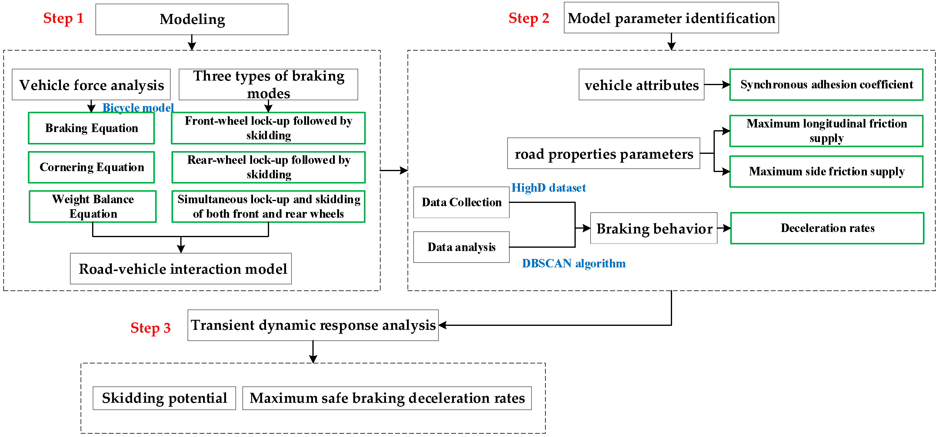
Figure 1. Flowchart of the research method.
Applsci 14 09357 g001
Figure 2. Forces acting on a vehicle on a horizontal–vertical combined curve: (a) a vehicle braking on a downgrade; (b) a vehicle cornering on a horizontal curve. Note: G is gravity, N; G = mg. The red dot represents the center of gravity.
Applsci 14 09357 g002
Figure 3. Variation curve of front- and rear- axle braking (or brake) forces. Braking force is the braking force of the ground acting on the wheel; brake force is the braking force of the brake acting on the wheel; β curve is the actual brake force distribution curve; I curve is the ideal brake force distribution curve; F line is the relationship between the front- and rear-axle braking forces in the case of front-axle lock-up; and R line is the relationship between the front- and rear-axle braking forces in the case of rear-axle lock-up. The specific meanings of the parameters can be found in Appendix A.
Applsci 14 09357 g003
Figure 4. Variation curve of front- and rear- axle braking (or brake) forces. The specific meanings of the parameters can be found in Appendix A.
Applsci 14 09357 g004
Figure 5. Variation curve of front- and rear- axle braking (or brake) forces. The specific meanings of the parameters can be found in Appendix A.
Applsci 14 09357 g005
Figure 6. Parameter identification procedure.
Applsci 14 09357 g006
Figure 7. Data analysis results for each highway section.
Applsci 14 09357 g007
Figure 8. Data analysis results for all highway sections.
Applsci 14 09357 g008
Figure 9. Prediction of truck skidding potential and recommendations of the MSBDRs on horizontal curves with different curve radii. Note: The area highlighted in orange indicates a high potential of skidding.
Applsci 14 09357 g009
Figure 10. Prediction of truck skidding potential and recommendations of the MSBDRs on horizontal curves with different slopes. Note: The area highlighted in orange indicates a high potential of skidding.
Applsci 14 09357 g010
Figure 11. Prediction of truck skidding potential and recommendations of the MSBDRs on horizontal curves with different friction coefficients. Note: The area highlighted in orange indicates a high potential of skidding.
Applsci 14 09357 g011
Figure 12. Prediction of truck skidding potential and recommendations of the MSBDRs on horizontal curves at different driving speeds. Note: The area highlighted in orange indicates a high potential of skidding.
Applsci 14 09357 g012
Table 1. Braking behavior parameter identification.
Classification of Braking BehaviorsRanges of Deceleration
(Algebraic Value)
Unit
Car-following braking [0, 1)m/s2
Stopping-sight-distance braking [1, 3)m/s2
Significant braking [3, 4.5)m/s2
Emergency braking [4.5, 5]m/s2
Table 2. Parameter values.
Influence FactorParameterSymbolValueUnit
VehicleMass m 30,000kg
Height of the CG h g 1.8m
Synchronous adhesion coefficient φ 0 0.4
Front axle to CG distance a 3.60m
Rear axle to CG distance b 4.25m
RoadDesign speed V D S 120/100/80km/h
Radius R 650/400/250m
Superelevation i h 8%
Downgrade i 0%
Friction coefficient (tire–pavement) μ x , m a x 0.6
EnvironmentWeather Dry
Driver behaviorSpeed V 120/100/80km/h
Deceleration a x 0~5.5m/s2
Note: The blue-filled areas indicate that the impact of changes in these variables on truck skidding is being explored.
Table 3. Parameter values.
Influence FactorParameterSymbolValueUnit
VehicleMass m 30,000kg
Height of the CG h g 1.8m
Synchronous adhesion coefficient φ 0 0.4
Front axle to CG distance a 3.60m
Rear axle to CG distance b 4.25m
RoadDesign speed V D S 80km/h
Radius R 250m
Superelevation i h 8%
Downgrade i 1/2/3/4/5/6%
Friction coefficient (tire–pavement) μ x , m a x 0.6
EnvironmentWeather Dry
Driver behaviorSpeed V 80km/h
Deceleration a x 0~5.5m/s2
Note: The blue-filled areas indicate that the impact of changes in these variables on truck skidding is being explored.
Table 4. Parameter values.
Influence FactorParameterSymbolValueUnit
VehicleMass m 30,000kg
Height of the CG h g 1.8m
Synchronous adhesion coefficient φ 0 0.4
Front axle to CG distance a 3.60m
Rear axle to CG distance b 4.25m
RoadDesign speed V D S 80km/h
Radius R 250m
Superelevation i h 8%
Downgrade i 0%
Friction coefficient (tire–pavement) μ x , m a x 0.6/0.5/0.44/0.34
EnvironmentWeather Dry/wet
Driver behaviorSpeed V 80km/h
Deceleration a x 0~5.5m/s2
Note: The blue-filled areas indicate that the impact of changes in these variables on truck skidding is being explored.
Table 5. Parameter values.
Influence FactorParameterSymbolValueUnit
VehicleMass m 30,000kg
Height of the CG h g 1.8m
Synchronous adhesion coefficient φ 0 0.4
Front axle to CG distance a 3.60m
Rear axle to CG distance b 4.25m
RoadDesign speed V D S 80km/h
Radius R 250m
Superelevation i h 8%
Downgrade i 0%
Friction coefficient (tire–pavement) μ x , m a x 0.6
EnvironmentWeather Dry
Driver behaviorSpeed V V D S /1.1 V D S /1.2 V D S km/h
Deceleration a x 0~5.5m/s2
Note: The blue-filled areas indicate that the impact of changes in these variables on truck skidding is being explored.
Table 6. Recommended maximum deceleration values.
ConditionHorizontal Curves with a Limit-Minimum-Radius
Compound condition/Steep slopesExtremely wet roadMore than 1.2 V D S
MSBDRs (m/s2)4.54.02.03.0
Disclaimer/Publisher’s Note: The statements, opinions and data contained in all publications are solely those of the individual author(s) and contributor(s) and not of MDPI and/or the editor(s). MDPI and/or the editor(s) disclaim responsibility for any injury to people or property resulting from any ideas, methods, instructions or products referred to in the content.