A Methodology Based on Deep Learning for Contact Detection in Radar Images

Abstract

Ship detection, a crucial task, relies on the traditional CFAR (Constant False Alarm Rate) algorithm. However, this algorithm is not without its limitations. Noise and clutter in radar images introduce significant variability, hampering the detection of objects on the sea surface. The algorithm’s theoretically Constant False Alarm Rates are not upheld in practice, particularly when conditions change abruptly, such as with Beaufort wind strength. Moreover, the high computational cost of signal processing adversely affects the detection process’s efficiency. In previous work, a four-stage methodology was designed: The first preprocessing stage consisted of image enhancement by applying convolutions. Labeling and training were performed in the second stage using the Faster R-CNN architecture. In the third stage, model tuning was accomplished by adjusting the weight initialization and optimizer hyperparameters. Finally, object filtering was performed to retrieve only persistent objects. This work focuses on designing a specific methodology for ship detection in the Peruvian coast using commercial radar images. We introduce two key improvements: automatic cropping and a labeling interface. Using artificial intelligence techniques in automatic cropping leads to more precise edge extraction, improving the accuracy of object cropping. On the other hand, the developed labeling interface facilitates a comparative analysis of persistence in three consecutive rounds, significantly reducing the labeling times. These enhancements increase the labeling efficiency and enhance the learning of the detection model. A dataset consisting of 60 radar images is used for the experiments. Two classes of objects are considered, and cross-validation is applied in the training and validation models. The results yield a value of 0.0372 for the cost function, a recovery rate of 94.5%, and an accuracy rate of 95.1%, respectively. This work demonstrates that the proposed methodology can generate a high-performance model for contact detection in commercial radar images.

1. Introduction

Today’s application of radars has expanded considerably in both civil and military fields due to the progress in radar technology. Such is the case that state-of-the-art radars can be detected in all weather conditions during the day, night, and long distances [1]. The navigation radar provides visual output about the elements present in a navigation scenario, displaying the position and distance information for each element. However, the identification and location of targets of interest on the sea surface are affected by a high degree of variability in the radar imagery [2]. This is due to several factors, such as weather conditions, alterations in the height of sea waves, land portions, birds, and noise caused by electronic interference [3,4].

Therefore, the search for a detection model that allows discarding unwanted echoes and detecting targets of interest with accuracy and low computational cost is a complex task, made even more so with commercial radars due to their limitations in terms of range, resolution, and reliability compared to military radars [5]. Nevertheless, detecting objects on the sea surface is of great interest for its application in civilian operations such as the timely rescue of vessels, maritime security, and the surveillance of the Peruvian coast [1,6,7,8].

Many commercial radars use the adaptive algorithm CFAR (Constant False Alarm Rate) in its various variants to establish the detection threshold. This algorithm presents a non-zero false alarm rate (PFA) [9]. The noise power is estimated from neighboring cells, and a dynamic detection threshold is set to match the data. The most used detector CFAR is the averaging of neighboring cells, calculated at a constant CUT (Cell Under Test) distance [10,11,12]. Experimentally obtained data from the radar installed on the vessel show a false negative rate of 0.05 and a false alarm rate of 0.10, especially in the images of regions containing sea and land in navigation parallel to the coast. To decrease this effect, the CFAR result is combined with other algorithms; multihypotheses and filtering with navigation maps are applied, significantly increasing the computational burden. In addition, for safety reasons, it is preferred to adjust. The constant CFAR parameters are used to reduce the false negative rate. However, this implies increasing false alarms, an effect that is compensated for by predictive algorithms combining the results of other antenna spins, inevitably increasing the computational cost [13,14].

On the other hand, modern methods based on deep learning algorithms are abstract feature-based methods that detect ships using features such as shadows, contours, and textures, which are extracted through deep convolutional neural networks (CNNs), achieving better detection performance than the traditional method [15]. This second group of methods can be classified into two-stage and one-stage detectors. Two-stage detectors are represented by the series of region-based convolutional neural networks (R-CNNs), which later evolved into Fast R-CNN and Faster R-CNN [16,17]. Faster R-CNN is distinguished by its two-stage process, where it first generates region proposals and then classifies those regions into object categories; due to the unification of the regional proposal and detection networks in a single model, it has turned out to be faster than its predecessors [18,19]. These models have the advantage of recognizing different types of objects more accurately, overcoming the problem of multiscale and multiscene detection [20,21,22]. Despite their complexity, two-stage detectors are favored for their high accuracy and robustness in object detection tasks [23,24,25].

Indeed, the single-stage detectors such as Single-Shot Multibox Detector (SSD) [26] and You Only Look Once (YOLO) [27] work much faster than two-stage detectors [28,29]. However, they compromise on accuracy, being insufficient when it comes to small objects [30,31], images with a lot of noise with scenarios with many background clouds, low resolution data where contour processing must be processed, and gray level distributions to distinguish the target [32]. While YOLO and SSD single-stage detectors excel in providing real-time processing and fast inspection capabilities, these may not always offer precise location for specific objects of interest [33,34]. Lately, several research works have been carried out to mitigate the effects of adverse visual conditions on object detection and demonstrate that YOLO architectures may be best suited for object detection under adverse visual conditions, such as rain, sunset, day or night. However, it should be noted that R-CNN models, despite their significant computational costs, have proved to be the most suitable for nighttime detection [35]. Faster R-CNN demonstrates its exceptional precision when locating objects at sea in conditions of very low visibility.

The recent research of [36] entitled “Faster R-CNN, RetinaNet and Single Shot Detector in different ResNet backbones for marine vessel detection using cross polarization C-band SAR imagery” confirms that Faster R-CNN and SSD show different capabilities in marine vessel detection. Faster R-CNN stands out as the best detector. This study shows that as the complexity of the ResNet backbones and the number of epochs increases, the accuracy of the model improves (100 epochs: Faster R-CNN = 0.67–0.70 mean F1 score; RetinaNet = 0.00–0.68 mean F1 score; SSD = 0.18–0.34 mean F1 score). Regarding the processing time, Faster R-CNN with different ResNet backbones takes longer to train for 100 epochs (1 h and 3 min) compared to other detectors (RetinaNet = 58 min; SSD = 44 min). Table 1 shows some results on the accuracy and processing time of marine vessel detection models (100 epochs) extracted from the work of [36].

Table 1. Results of marine vessels detection models (100 epochs).

Algorithm	Backbone	Accuracy				Processing Time
		Precision	Recall	F1 Score	mAP
Faster R-CNN	ResNet34	0.90	0.68	0.77	0.21	0:50:41
	ResNet50	0.82	0.83	0.82	0.23	00:53:20
	ResNet101	0.85	0.85	0.85	0.27	01:25:39
Retina Net	ResNet34	0.08	0.01	0.01	0.00	00:42:22
	ResNet50	0	0	0	0.00	00:57:52
	ResNet101	0.74	0.74	0.74	0.14	01:14:46
SSD	ResNet34	0.30	0.09	0.14	0.01	00:28:32
	ResNet50	0.44	0.24	0.31	0.02	00:43:19
	ResNet101	0.49	0.31	0.38	0.03	01:00:25

Source: Adapted from Altarez (2024) [36].

In another research work [37], three different object detectors were tested: one two-stage detector (Faster R-CNN) and two single-stage detectors (YOLO v3, SSD). This choice was made to make a comparison between the increased speed typically seen in single-stage approaches and increased accuracy often achieved by two-stage approaches. For all image resolutions, Faster R-CNN using ResNet-50, 101 and 152 achieved the three highest F1 scores, reporting a maximum F1 score of 0.82 on their shrub detection. Table 2 shows shrub species detection for different deep learning methods extracted from the work [37].

Table 2. Results of shrub species detection accuracy for different deep learning methods.

Object Detector	CNN Architecture	Precision	Recall	F1 Score
Faster R-CNN	ResNet50	0.692	0.819	0.749
	ResNet101	0.680	0.777	0.723
	ResNet152	0.655	0.774	0.709
YOLOv3	DarkNet53	0.592	0.659	0.619
SSD	ResNet50	0.559	0.531	0.543
	ResNet101	0.547	0.513	0.527
Faster R-CNN	ResNet34	0.440	0.426	0.423

Source: Adapted from Retallack et al. (2022) [37].

Based on the literature, it is shown that two-stage object detectors achieve higher accuracy at the expense of the processing speed. On the other hand, detectors with single-stage approaches, such as YOLO and SSD, are more suitable for real-time processing.

The purpose of our research is to demonstrate that a new detection algorithm approach, based on deep learning, can improve the radar detection system currently used by the Peruvian Navy, CFAR. Faster R-CNN has been selected for other single-stage detectors for two reasons: (1) First is the deficiencies of the current CFAR model to monitor and detect marine vessels in scenarios with complex weather conditions of the Peruvian coast. The deficiencies are reflected in a false alarm rate of 0.10 and false negative rate of 0.05 in images of regions parallel to the beach. (2) Second is the radar infrastructure installed on Peruvian Navy vessels. Therefore, our choice is mainly focused on detection accuracy over real-time processing.

In this study, a methodology is designed for the detection of vessels of different shapes and sizes on the Peruvian coast, using original radar images owned by the Peruvian Navy. The present work estimates the performance, in terms of accuracy and speed, of new detection models based on deep learning. While object detection is a well-established field, this study is novel, as it examines this new approach for the first time. It is conducted on one of the most important ports of Peru, called Callao.

This article describes the complete methodology for contact detection. The convolution techniques applied and the parameters defined for the preprocessing and enhancement of radar images are detailed. In the second phase, the artificial intelligence techniques used to obtain cuts of objects of interest in an automated manner and the criteria that were considered for more efficient labeling are described. Subsequently, the design of the experiments and training using deep learning algorithms based on the Faster R-CNN architecture is described. The hyperparameter tuning values are specified below. Finally, the discrimination process is detailed according to the criteria defined by the radar expert to obtain the persistent objects called plots. The experiments with the Faster R-CNN model demonstrate favorable results with an average F1 score of 0.95, which demonstrates the model’s ability to recover more objects and with high precision.

The rest of the paper is organized as follows: Section 2 presents the detection system in the Peruvian Navy; Section 3 describes the methodology; Section 4 presents the experiments and the analysis of the results; Section 4 presents future work; and Section 5 presents the conclusions.

2. Detection System in the Peruvian Navy

The Peruvian Navy has several surface search radars, such as RAN-11X, RAN-105 and Sperry Marine. The radar detection system comprises two critical processes: (1) extracting plots (a plot is the term used to identify an object, called a contact or target in the military context; in the survey, it represents a marine vessel), and (2) tracking and prediction. Figure 1 shows the diagram of the detection system processes.

Figure 1. Detection system processes flow chart.

2.1. Phase 1: Plot Extractor

In the first phase, videos of radar images are received as input. The raw data originate from an echo, a bounce of the electromagnetic signal emitted by the radar. The radar movement is performed in turns of 0.17578°, so 2048 echoes are obtained in 360° or one radar turn. The radars used have a range of 150 km, receiving a total of 8192 analog samples as video. In this phase, three processes are executed to extract the plots. The processes are explained below:

2.1.1. Digitization of Radar Turn

Each echo is reflected as a line on the radar image and represents an azimuth. Each line comprises several samples corresponding to the maximum range of the radar, called the range. The data received from an echo are read and converted into digital format. The data are stored in memory until the 2048 echoes of a radar lap are completed. This way, a raw image is obtained, which is processed in the next step.

2.1.2. Preprocessing

In preprocessing, the image is cropped to a certain dimension. In this stage, different convolutions are applied to the radar images in order to eliminate the interference caused by noise. The Gaussian filter and the arithmetic mode are used to obtain cleaner images. The images are then normalized and sent to the plot detection process.

2.1.3. Plot Detection

This process involves the extraction of plots using detection algorithms. The detection algorithm used by the Peruvian Navy for the last 20 years is based on the CFAR statistical method, designed with a variation and simplification to one line. The CFAR algorithm is used in a single dimension, applying the detector to each echo in a given angular direction, from 0° to 360°. This detector model is enabled on many commercial ships and defense systems. The CFAR detector receives the echoes, detects pixel strings, and obtains probabilities to determine whether it is a contact. If the detected strings in one line are adjacent to any string in the following line, an object is formed; when the object no longer has adjacent strings, the object detection process is terminated. This process is executed in real-time and ends when the extracted plots are sent together with the metadata, center of gravity, and area to the second phase, called Tracking-Prediction. However, the CFAR detection algorithm presents certain deficiencies reflected in the data obtained experimentally from the radar installed on the vessel, equivalent to a false alarm rate of 0.05 and false negatives of 0.10.

Our research is framed within this plot detection process. This process is crucial because it requires extracting as many plots as possible, which will then be processed to determine the defense operations. The improvement in this process results in the accurate detection of plots that will be extracted to continue their course in the next phase. The processes corresponding to each phase are shown in Figure 2. The process that frames our research is highlighted.

Figure 2. Processes of plot extractor phase flow chart.

2.2. Phase 2: Tracking-Prediction

The second phase comprises two processes: (1) tracking and (2) prediction. In this phase, the extracted plots are monitored. The movements made along the track are evaluated to determine its course and velocity. Predictive algorithms are used to obtain the future position; the correlation between the past, current, and arrival times at the defined target points or contact points is analyzed.

The objective of the our work is to prove that a new algorithm model based on deep learning can achieve better performance than the existing CFAR algorithm. Consequently, it improves the efficiency of the radar detection system. Currently, the CFAR algorithm is operational. In addition, radar vessels present the infrastructure designed to execute real-time operations. The state of the art concerning artificial intelligence-based models is focused on selecting models that would provide higher accuracy performance in marine contexts over speed. We review new approaches to object detection, which offer better performance, increasing the ability to obtain more plots (recall) with a high degree of precision (accuracy). Therefore, we prioritize models that provide higher performance in accuracy over speed.

2.3. Radar System Architecture

Plot detection is a real-time process and requires both immediate and accurate responses. Real-time processes and hardware have a critical relationship [38]. Depending on the hardware components used, fast and permanent access to memory, reliable storage mechanisms, and high speed of operation can be guaranteed. Consequently, it can be said that the radar system’s architecture influences the performance of capturing, transmitting, processing, detecting, and tracking contacts. The infrastructure used in the Peruvian Navy includes VME (Versa Module Eurocard) Host Processor cards, PMC or Mezzanine Cards for radar data input, scanning converters, and graphics cards integrated with PCI (Peripheral Component Interconnect) communication buses. Each vessel with navigation radars consists of 32 multicore processors, including 16 backup processors. The hardware, together with the middleware software and the CFAR plots detection algorithm, which are currently running, respond within the established minimum latency time. However, CFAR has shortcomings in the rate of false alarms and false negatives. The objective of this work is to search for a contact detection algorithm that exceeds the accuracy capability of the current CFAR algorithm. Therefore, the predominant factor in evaluating and choosing the new detection model is the accuracy capability over speed. Figure 3 shows the radar system architecture diagram.

Figure 3. Radar system architecture.

3. Methodology

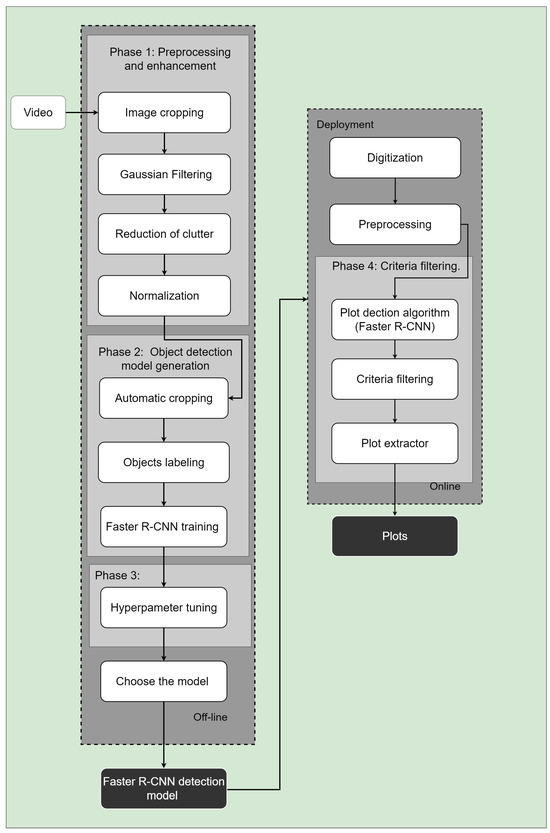
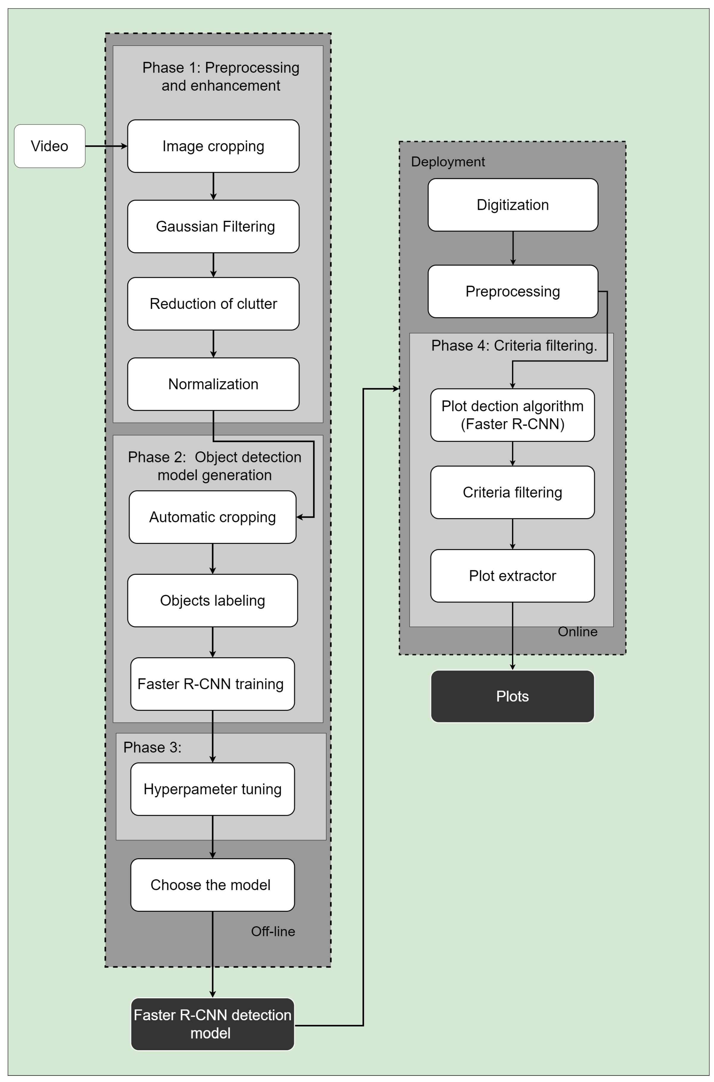
The methodology used for object detection is based on the application of artificial intelligence and incorporates a series of processes, methods, and techniques to obtain persistent objects called plots or contacts in radar images. The methodology comprises four phases: image preprocessing and enhancement, object detection model generation, hyperparameter tuning, and criteria filtering. The first phase consists of radar image preprocessing and enhancement using convolution techniques. The second phase covers automatic cropping. Labeling is assisted with a proprietary interface, and training is performed using the Faster R-CNN model. In the third stage, model tuning is performed, evaluating the relevant metrics obtained because of a series of combinations of hyperparameters, and in the fourth phase, we present the execution of the plot detector with deep learning for use in real-time radar execution. In this phase, filters, which the radar expert determines, are added and executed to determine whether a plot is persistent and real, aiming to avoid false positives and improve performance. Figure 4 shows the methodology flow chart.

Figure 4. Methodology flow chart.

3.1. Phase 1: Preprocessing and Enhancement

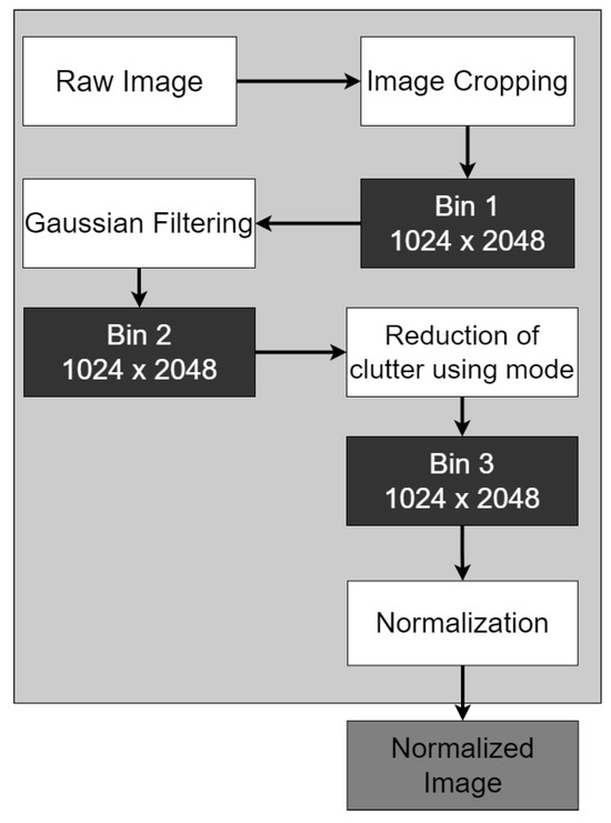
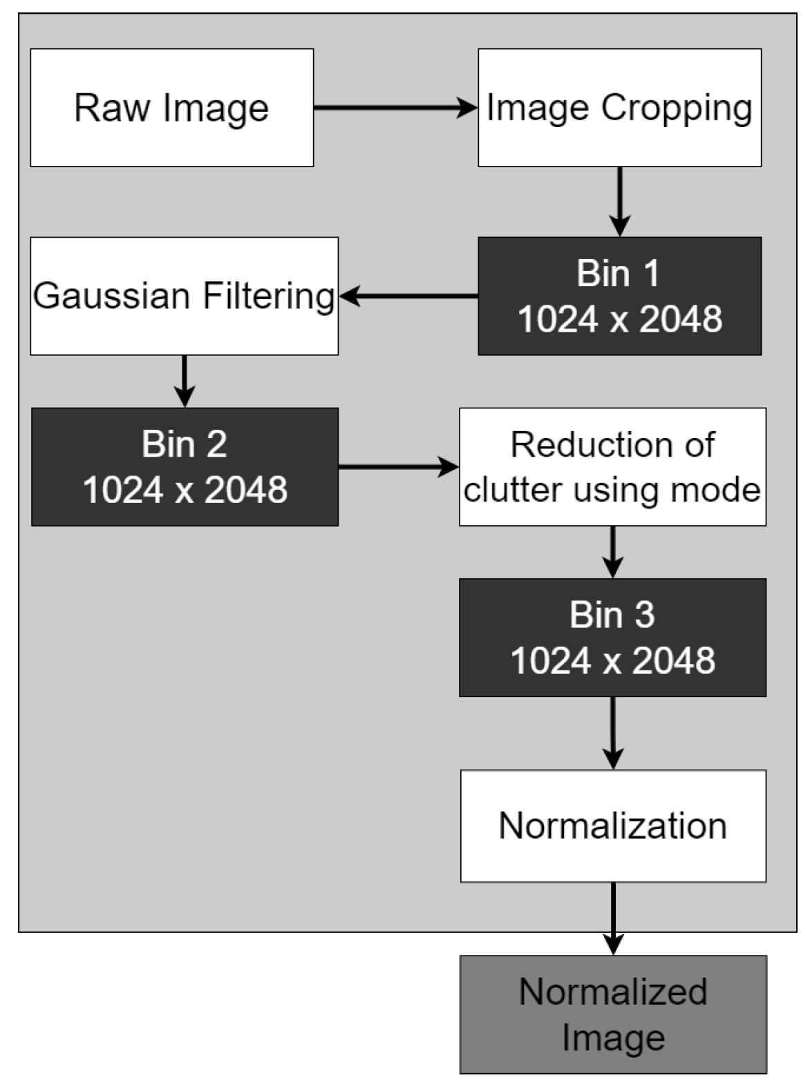
In the first phase, the images undergo an enhancement process. The images are cropped, and a file called bin1 is obtained. This bin1 file passes through a 1D Gaussian convolution filter. The Gaussian filter smooths the image, eliminates interference caused by noise, and obtains the bin2 file. The next step is to apply the arithmetic mode of the complete image to obtain a bin3 file; this is performed to reduce the intensity of possible false positives caused by interferences. Finally, the images are normalized and sent to the following phase. After performing several tests, we establish specific parameters. The parameters provided ensure a better quality of commercial radar images, which will be used in the training with deep learning algorithms. The processes of the first phase are shown in Figure 5.

Figure 5. Preprocessing and enhancement phase flow chart.

3.1.1. Image Cropping

First, the raw image is cropped to a size of 1024 × 2048. This decision to crop the image is because, for this study, we only consider analyzing a distance of 37.5 km, which is equivalent to 2048 samples of the 8192 provided by the radar. After all, the vessel requires only the analysis up to this distance to be used, and thus, the computational overhead is also avoided. Likewise, the decision to take only 1024 azimuths is made since, in the middle zone of the image, the highest probability of observing a contact is established, so in the clipping process, only the average azimuths of the entire radar image are chosen. Therefore, if we analyze that there are 2048 azimuths and we number them from 1 to 2048 when clipping, the samples from azimuth 513 to azimuth 1536 are selected. So, azimuth 1 to 512 are eliminated, and azimuth 1537 to 2048 are eliminated. In this process, we obtain the bin1 file.

3.1.2. Gaussian Filtering

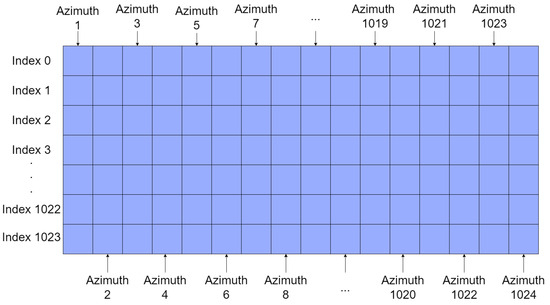
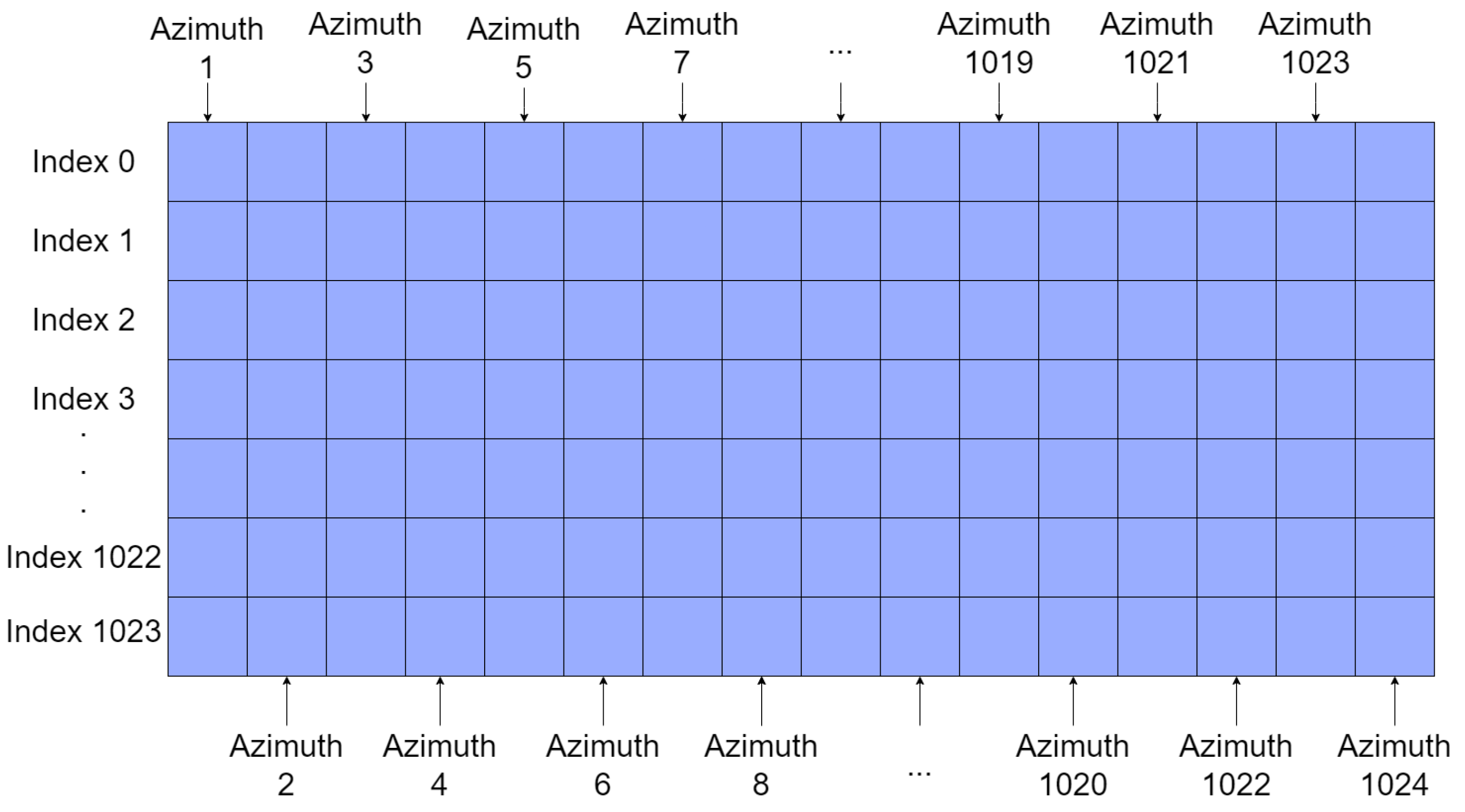
The bin1 file is passed through a Gaussian filter in 1D (one dimension). Each line of the radar image is taken as if it were a signal. To explain this, we can look at the radar image as a matrix, where the columns represent the azimuths, and the rows represent the different values at a given point in space for each of the azimuths as shown in Figure 6.

Figure 6. Radar image structure as matrix. Each column is an azimuth, and each row is the distance value given to all azimuths. Each index row starts with 0.

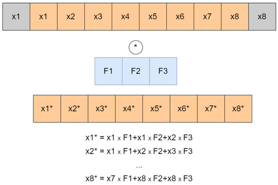
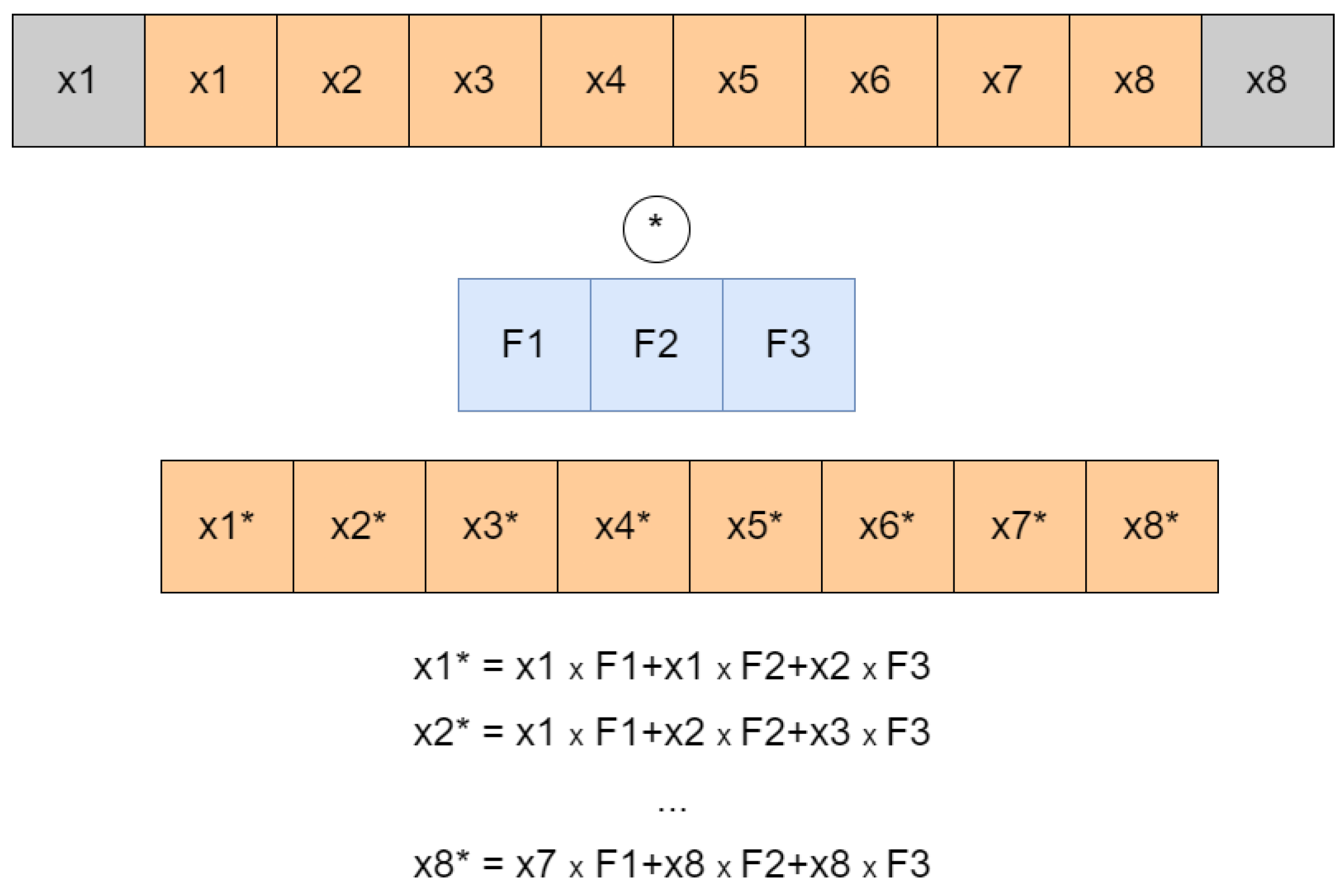
For example, if we analyze the row with index 0, the first line, we will see the value taken at the distance of 37.5 km for all azimuths from 1 to 1024. When referring to the index, we are talking about a matrix position usually read starting with 0. If we take the index row 1, it would be the values at a distance of 37.48 km for each azimuth. So, each row can be represented as a signal or a vector of size 1024 for this case. Taking each row as a vector of 1024 values is better for visualizing the following convolution process. The convolution filter is one-dimensional because each row of the radar image is 254 convoluted with the filter and then moved to the next row. The one-dimensional convolution is depicted in Figure 7.

Figure 7. Representation of a convolution in 1 dimension. * has been placed to represent the output value of the corresponding vector at that index, after convolution. Example: x1* is equal to the resulting convolution at the index where x1 was without *.

An 8-term signal convoluted with a 3-term filter can be assumed in a convolution representation. Note that the terms at the ends are repeated to keep the dimension of the output signal the same as the dimension of the input signal. This technique, called padding, is used to avoid the output signal, being smaller than the input signal. If this technique is not used, the output signal would have only six terms instead of eight.

A signal smoothing filter is the Gaussian filter. The purpose of a smoothing filter is to reduce the noise caused by high-frequency disturbances in a signal. The Gaussian probability equation is seen in Equation (1):

$$\begin{array}{c}\hfill f(x;\mu ,\sigma )={\displaystyle \frac{1}{\sqrt{2\pi \sigma }}}{e}^{-{\displaystyle \frac{1}{2}}{{\displaystyle \frac{(x-\mu )}{\left(\sigma \right)}}}^2}\end{array}$$

(1)

where x is the data to be evaluated, $\mu$ is the mean, and $\sigma$ is the standard deviation. For one dimension and choosing a mean equal to 0, we have Equation (2):

$$\begin{array}{c}\hfill G\left(x\right)={\displaystyle \frac{1}{\sqrt{2\pi \sigma }}}{e}^{-{\displaystyle \frac{1}{2}}{{\displaystyle \frac{\left(x\right)}{\left(\sigma \right)}}}^2}\end{array}$$

(2)

The constants $K_1$ and $K_2$ are then defined for the calculation of each point of the convolution filter as shown in Equations (3) and (4):

$$K_1={\displaystyle \frac{1}{\sqrt{2\pi \sigma }}}$$

(3)

$$K_2=-{\displaystyle \frac{1}{2{\sigma }^2}}$$

(4)

$K_1$ belongs to the right-hand constant of the equation, and $K_2$ is the exponent of the expression.

Once the constants are replaced in Equation (2), the new equation is shown in (5):

$$\begin{array}{c}\hfill G\left(x\right)=K_1{e}^{k_2{x}^2}\end{array}$$

(5)

So, as a filter, we use a vector that follows the Gaussian likelihood ratio so that the central value in the convolution vector is $x=0$. The best way to perform this is to consider a value $Lk$. This value will be the points within the Gaussian distribution to be taken for each side of the mean. For example, if $Lk=3$, seven values will be taken, where the central value will take the maximum value of the Gaussian equation. This $Lk$ value, therefore, returns a convolution vector with $2\ast Lk+1$ values representing a Gaussian distribution to eliminate noise in the radar image signal. Several equations can be used to choose the value of $Lk$, like the equations proposed in (6) and (7):

$$Lk=round\left(F_{TK}{\displaystyle \frac{e^2\sigma +\frac{\sqrt{2\pi }}{\sqrt{e}}}{2}}\right)$$

(6)

$$Lk=round\left(F_{TK}{\displaystyle \frac{7.39\sigma +1.284}{2}}\right)$$

(7)

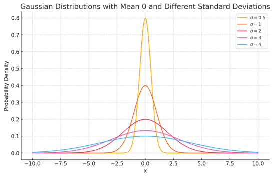
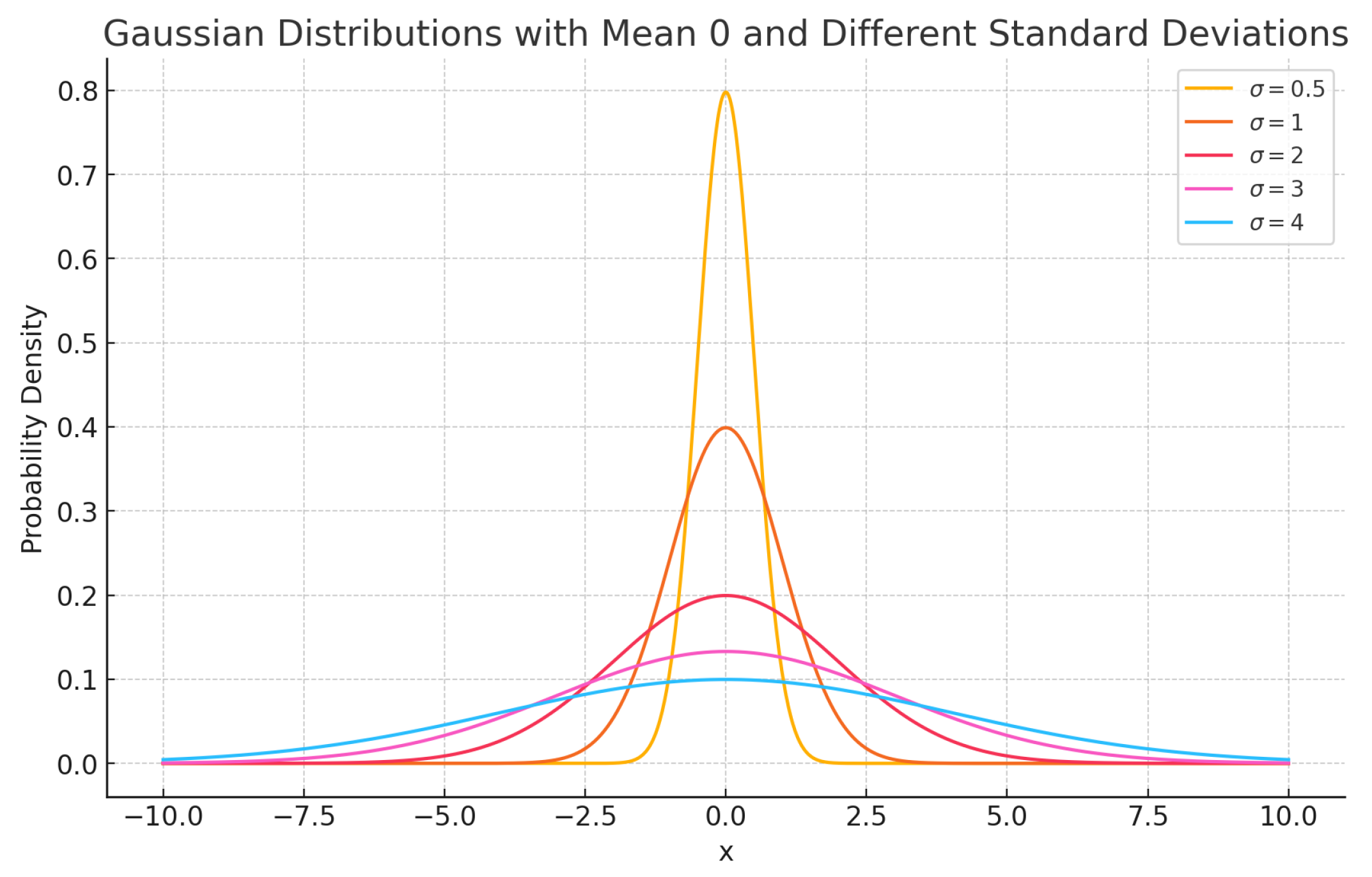
where $F_{TK}$ is a mass approximation constant; if $F_{TK}$ is high, it will capture a large percentage of the Gaussian distribution. However, the convolution vector will become unnecessarily large. The mean of the Gaussian distribution is 0, but one must evaluate and choose the values of $\sigma$ and $F_{TK}$. To determine the value of $\sigma$, Gaussian distributions are plotted with different standard deviations as seen in Figure 8. We see that a standard deviation of 2 causes an attractive weighting effect for the study.

Figure 8. Gaussian distribution with different standard deviations.

We can see that the curves are very steep for distributions with minimal standard deviations, so the weighting is not precise. A steep weighting is sought, meaning the mean term should be high while the non-mean term should be low. We see that with a standard deviation equal to 2, this effect is primarily achieved. For larger deviations, since the distribution curve is so smooth, we also have the same problem as when the distributions are very low, which is that there is no effective weighting; therefore, the choice of $\sigma =2$ makes a lot of sense. Likewise, let us evaluate, once $\sigma =2$ is already chosen, possible values of $Lk$ for different $F_{TK}$. If we choose a very high $F_{TK}$, we will have an unnecessarily large filter, so our $F_{TK}$ should be around 0.7 to 1. With 0.8, we obtain a filter with 13 values, sufficient to perform the convolution in 1D. Thus, if we find the 13 values that comprise the selected convolution vector, we can obtain this vector in (8):

$${Gauss}_{LK}=\left[0.0004,0.054,0.0270,0.111,0.2417,0.3989,0.500,\dots 0.004\right]$$

(8)

The 13 values have not been placed due to being symmetrical after 0.5.

They are repeated so that the nearest value is 0.3989, and so on. The result of this convolution between the image and this Gaussian vector will be the bin2 file.

3.1.3. Reduction of Clutter

Subsequently, the bin2 output goes through a convolution process called Mode&clutter to reduce the clutter. As a result, the output bin3 is obtained by applying the following algorithm to the resulting matrix. It can be expressed in (9) and (10):

$$bin{3}_{az,s}=\left\{\begin{array}{cc}0& \hfill bin{2}_{az,s}<=\mu \\ bin{2}_{az,s}-\mu & \hfill Otherwise\end{array}\right\}$$

(9)

$$\mu =mode\ast clutter$$

(10)

where we have the following:

• $mode$: The statistic mode of the region defined between the 200 and 800 azimuths from samples 300 to 1024.
• $clutter$: This factor reduces noise and is settled at 2 values.
• $\mu$: It is a threshold that measures the minimum amount of noise that is affecting the whole image or the minimum values of the image to have a clean final image so that the intensity of the detected objects is the only one that can be observed in the image.
• $bin3$: It is a decision matrix, where there is a threshold $\mu$ such that values below this threshold become 0, meaning they are not visible in the image. For values above this threshold, the threshold is subtracted from them.

• Consider the default values of 2 and 3 for the radar image’s upper and lower ranges, respectively. The selected range of the radar image comprised of this is represented as (11)

  $$From{\displaystyle \frac{1}{sub-range}}to{\displaystyle \frac{1}{2}}imagen$$

  (11)

The intensity per line is analyzed to choose a mode. The average intensity per line is considered to avoid choosing a too small mode. The process involves subtracting the mode of the clutter concerning the whole image.

3.1.4. Normalization

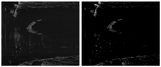
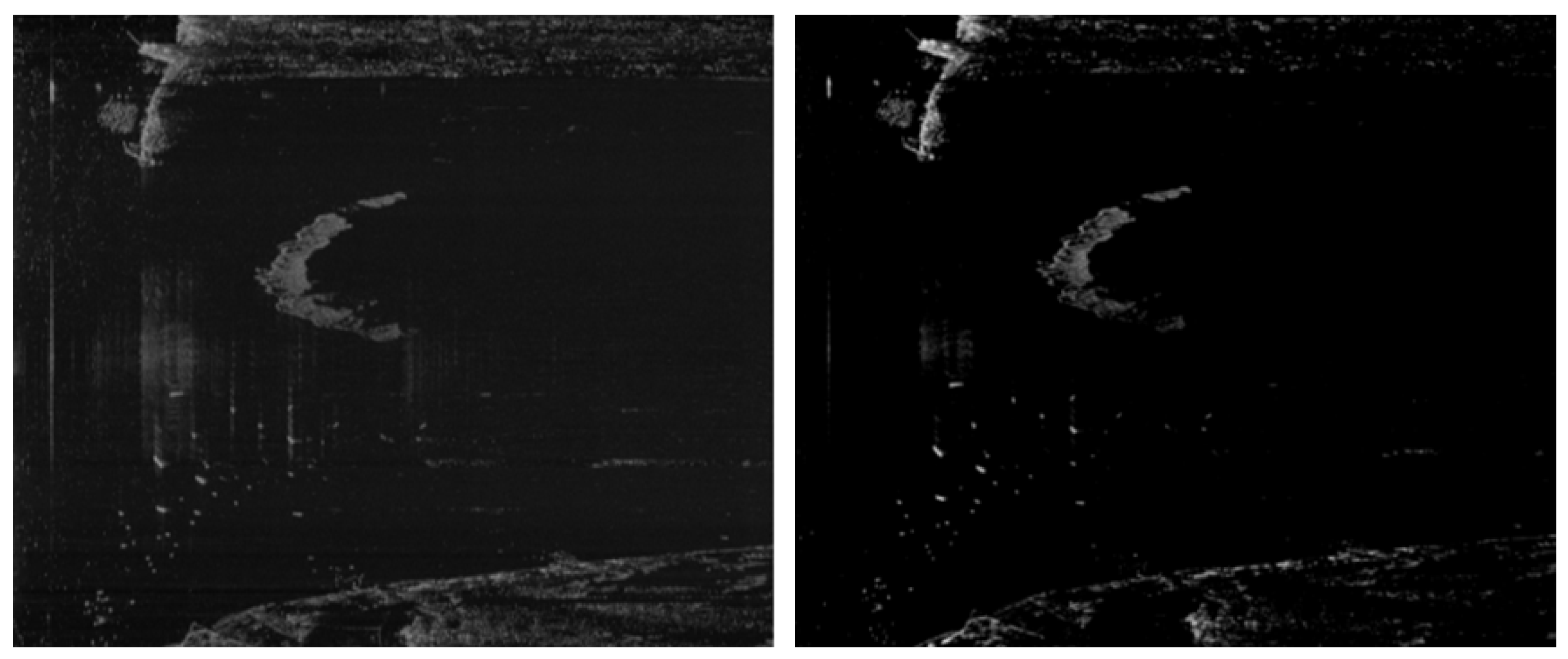
Finally, the bin3 output goes through a normalization process of the images between the values 0 and 255. The images have previously gone through a 1-channel to 3-channel gray scale conversion process. Figure 9 presents the raw image before the preprocessing and enhancement phase and the normalized image as a result or output of this first phase.

Figure 9. (Left) Sperry Marine radar raw image. (Right) Resultant normalized image after the preprocessing and enhancement phase.

3.2. Phase 2: Generation of the Object Detection Model

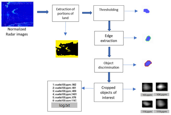
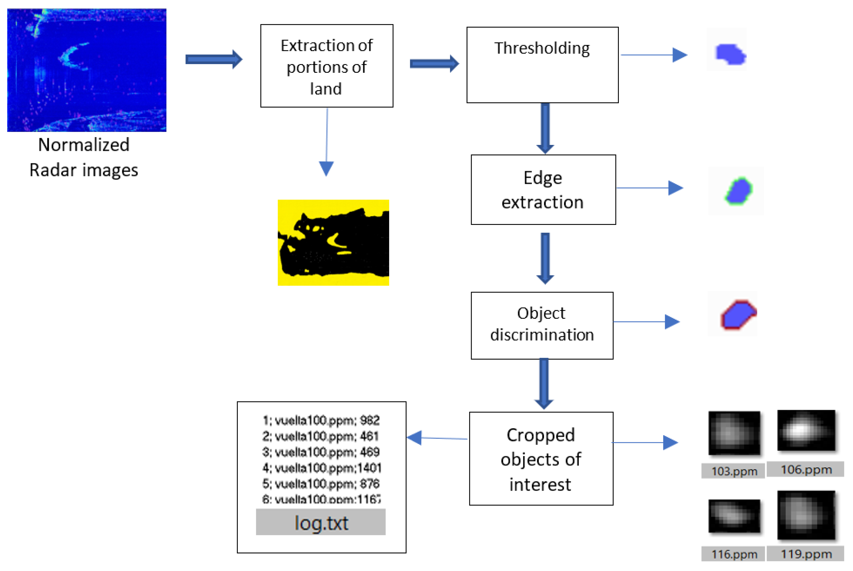
In the second phase, the normalized images go through an automatic cropping process to obtain cuts of objects that will be labeled. Later, these images are trained using the Faster R-CNN model. The processes of the second phase are shown in Figure 10. The processes are detailed below.

Figure 10. Automatic cropping flow chart.

3.2.1. Automatic Cropping

In this process, several artificial vision techniques are used to perform: edge extraction, considering the intensity values and the dimensions of the objects of interest. The edge extraction process is based on the work of [39]. First, land portions such as islands and coastal zones are removed using a template. Subsequently, thresholding techniques are applied within the image, considering the pixels corresponding to a specific range of intensity values. The intensity values considered correspond to the reflectivity or Radar Cross-Section of the objects of interest. Likewise, the width considered for edge extraction is a maximum of one pixel, which is convenient for obtaining the contour of the objects of interest. Then, the discrimination of the objects is performed, considering the dimensions of the desired objects (ships). Object discrimination results in the cutouts of the possible objects of interest together with their coordinates. The flow chart of the automatic cropping process is shown in Figure 10.

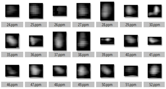
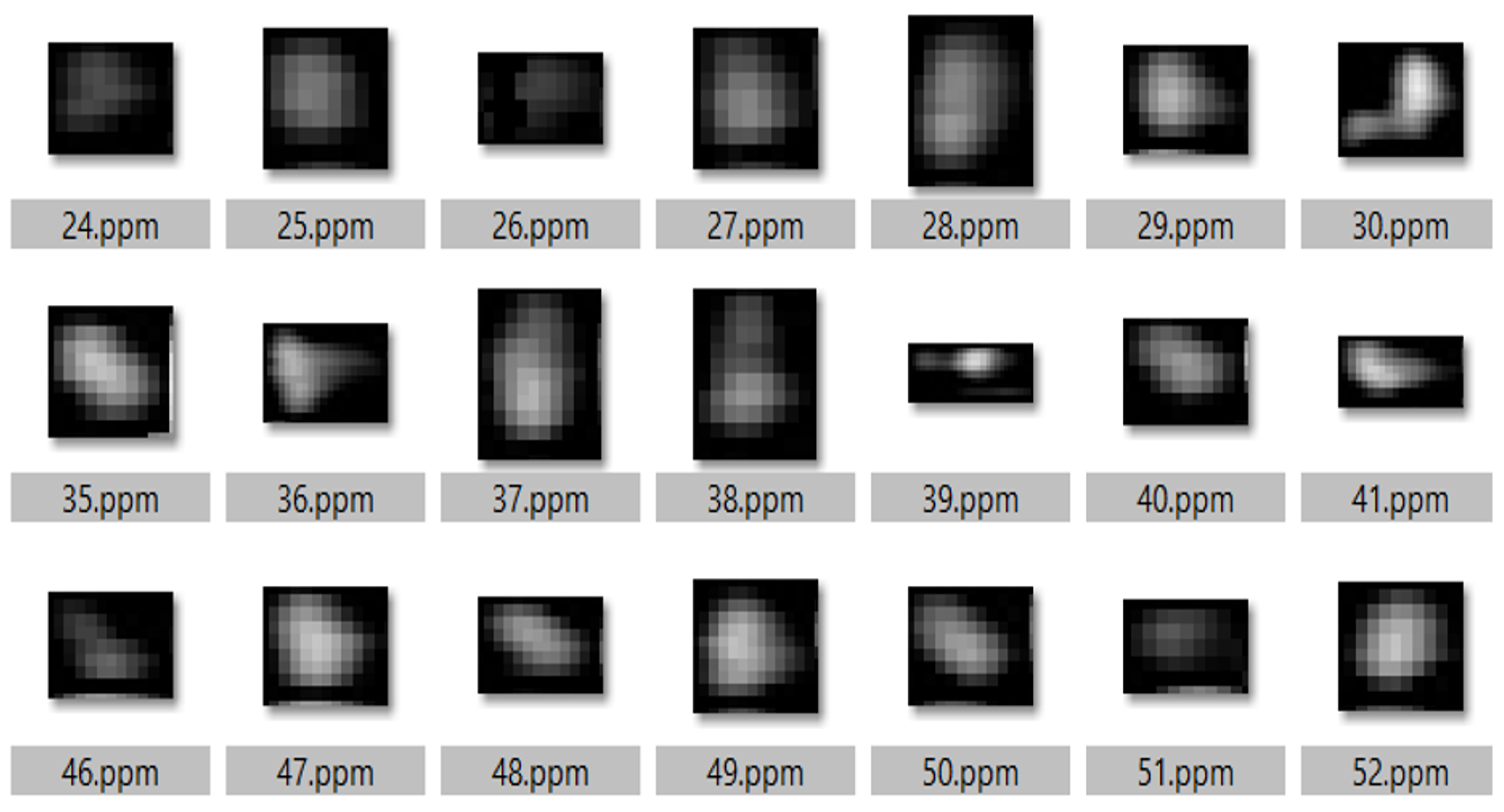
Figure 11 shows cuts of objects obtained through automatic cropping. These objects of interest are normalized to facilitate the next stage of classification and labeling by the expert.

Figure 11. Images of cutouts of objects.

With the cuts of objects of interest, the text file log.txt is generated. This file contains each of the cutouts of the objects of interest with x and y coordinates. The file contains the following fields:

• Filename: It is the identifier of the radar return.
• Xmin: left horizontal coordinate, between 0 and 2048.
• Xmax: right horizontal coordinate, between 0 and 2048.
• Ymin: upper vertical coordinate, between 0 and 1024.
• Ymax: lower vertical coordinate, between 0 and 1024.

3.2.2. Objects Labeling

Before the labeling process, a combination of characteristics or requirements is established based on rules [40]. The rules represent the expert’s knowledge to classify the two classes of objects of interest. An object is considered a ship if the cutout of the object of interest is positive, and will be labeled “plot”. Otherwise, if the clipping of the object is harmful, then it is not a ship and will be labeled “no”. This is represented as (12):

$$box=\left\{\begin{array}{cc}“plot”\hfill & \hfill \mathrm{this}\mathrm{is}\mathrm{a}\mathrm{contact}\sim ship\\ “no”\hfill & \hfill \mathrm{this}\mathrm{is}\mathrm{not}\mathrm{a}\mathrm{contact}\end{array}\right\}$$

(12)

For an object to be considered a “plot”, the rules established by the radar expert include persistence and completeness.

• Persistence in three consecutive turns means that the object appearing in the current round must be present in the previous and next round. This translates as follows:

  The object is present in the current round AND the same object is present in the previous round AND it is also present in the next round.

• Completeness of the object. This translates as follows:

  The object must contain a single echo AND the echo must be perfectly framed in the object cutout.

Likewise, for an object to be considered “no”, the following must occur:

The object is not persistent OR the object is not complete OR the object cutout partially contains the object OR the object contains overlapping elements OR any other type of ambiguous elements.

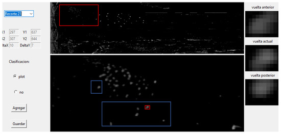
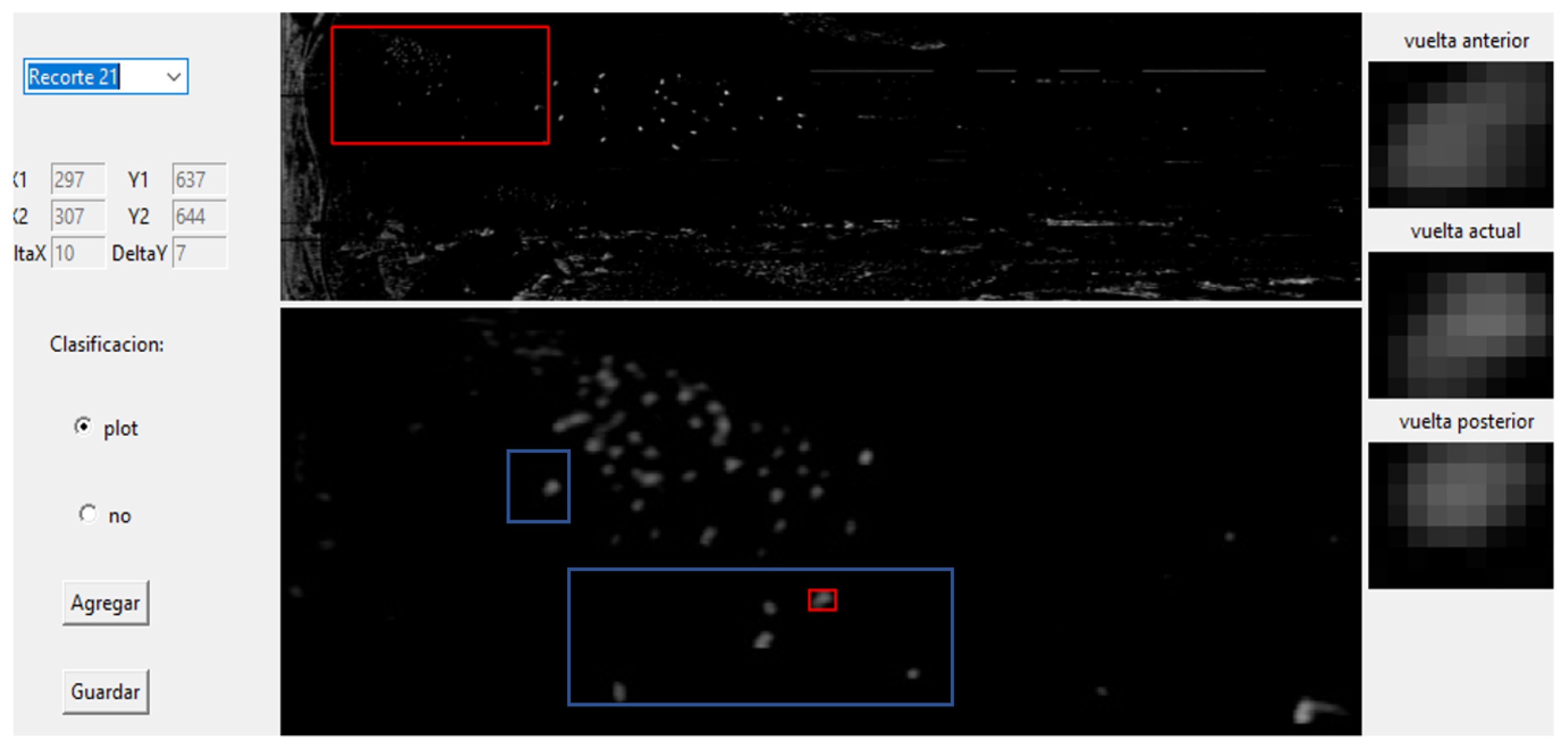
To carry out the labeling more efficiently, a proprietary labeling interface is developed with functionalities that make the process easier. This interface allows for visualization of the complete image and shows the clipping area and the clippings of objects of interest of three consecutive laps with their corresponding coordinates. The labeling process is carried out by a team of experts who apply the previously established rules.

In our previous works [41,42], the labeling process was performed with the tool LabelImg [43]. The time it took us to label an image of 50 objects was 60 min. With the developed labeling interface, it has been possible to visualize in parallel the images of the previous and next round, facilitating the application of the radar expert’s criteria. It has allowed to reduce the labeling time from 60 to 7 min, this means from 1.2 min to 8.4 s. The labeling time per radar image has been reduced by 88%. Figure 12 shows the labeling interface designed based on the rules of the radar expert.

Figure 12. Object labeling interface. The red box above corresponds to a zoom section in the radar image, this zoom section is displayed at the bottom of the figure. The blue boxes at the bottom of the figure represent regions of the radar image where it is possible to find a plot. The red box at the bottom is used to frame a current plot. On the right hand side we visualise this plot framed with red and check with the previous and next lap whether at the same location, at these coordinates, the same plot exists as a persistence criterion.

The labeling ends with the generation of the object of interest clippings and a text file with the coordinates of the bounding boxes of the objects of interest together with the class labels “plot” or “no”.

3.2.3. Faster R-CNN Training

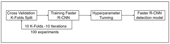
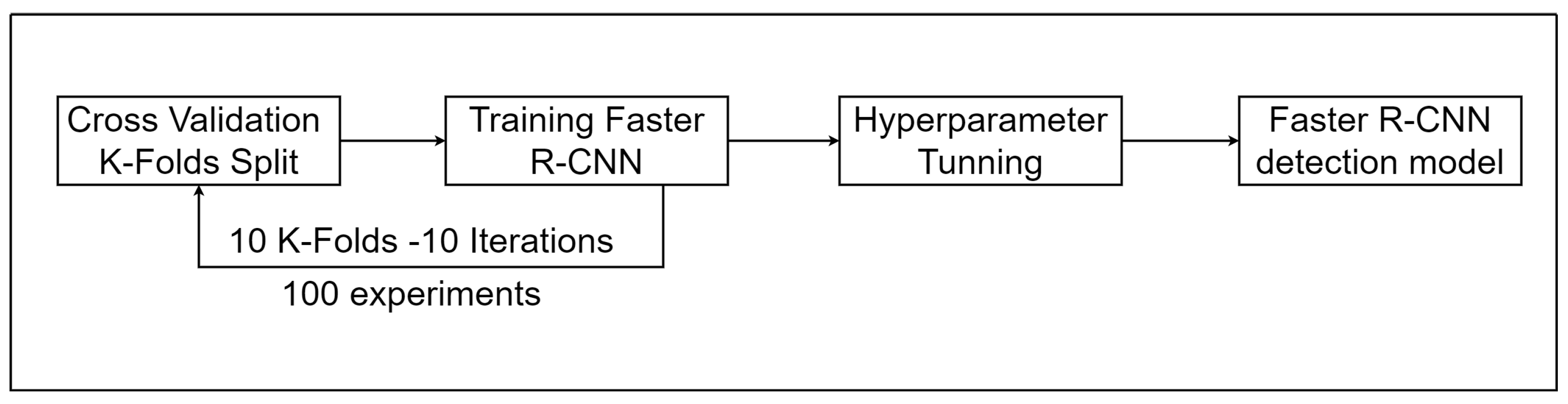
We employ Transfer Learning using the TensorFlow Object Detection Application Programming Interface (API) (API-TFOD). The training is performed using the Faster R-CNN Inception V2 architecture [44,45]. We choose the most suitable deep learning architecture by evaluating detection speed and accuracy. We choose Faster R-CNN Inception V2 as the base architecture for the possible alternatives. The reason for this choice is to prioritize the model that enables high performance in object detection accuracy, with a processing time that is no less important. Faster R-CNN Inception V2 meets this requirement, having achieved a throughput of 82% and a total processing time of 0.17303 s in previous work [41]. Figure 13 shows the training processes.

Figure 13. Training process flow chart.

3.3. Phase 3: Fine-Tuning of Hyperparameters

In this phase, some hyperparameters such as the learning rate, optimizer, and others are adjusted to improve the convergence rate of the model and optimize the model performance on inference dataset [42,46,47]. The methodology involved the selection of different combinations of hyperparameters. In previous work, experiments were carried out combining different values for IoU, batch-size, weight initialization, epochs and optimizer. Thus, it was determined that the initialization of the weights and the optimizer are the hyperparameters that act significantly in the learning of the detection model [48]. This aligns with other research works that demonstrate the influence of certain hyperarameters on model learning [49,50,51,52,53,54]. The values considered in the configuration file for the hyperparameters are shown in Table 3 and have been extracted from our previous work [48].

Table 3. Hyperparameter configuration.

Hyperparameter Configuration	Values
Epochs	100.000
IoU	0.6
Batch-size	2
Weight initialization	$\mu =0$; $\sigma =0.05$
Optimizer	ADAM

3.4. Phase 4: Criteria Filtering

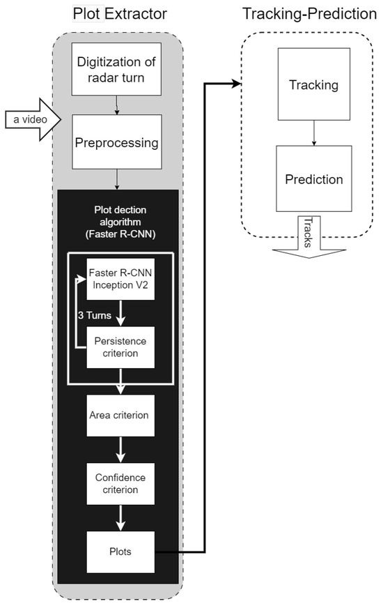
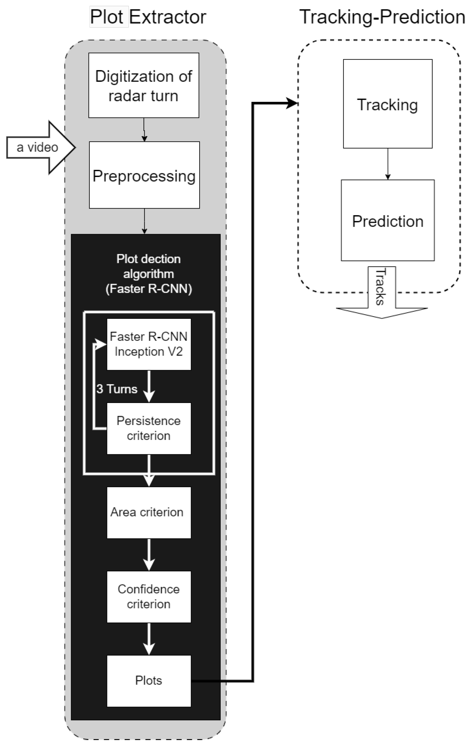
In the fourth phase takes place during the execution of the plot detector. The optimized detection model is run to obtain 1024 × 2048 output images with the objects of interest. A series of filters are applied to this output using three criteria to obtain the persistent objects. For an object of interest to be considered a persistent object, it must meet the following requirements:

• Persistence criterion: This criterion corresponds to the visibility of the target in three consecutive revolutions. To determine the persistence of the objects, a comparison is made based on a period of two radar revolutions; this measure is sufficient for declaring an object persistent in an oceanic context.
• Area criterion: All objects with dimensions greater than 30 × 30 pixels are discarded. This value corresponds to the maximum Radar Cross-Section area value of the objects of interest.
• Confidence criterion: Only clippings of objects with a probability more significant than the threshold of 0.85 are considered, this being the value established to determine that the object is contained in the clipping.

Figure 14 shows the processes of the criteria filtering phase.

Figure 14. Criteria filtering phase flow chart.

4. Experiments and Analysis of Results

4.1. Dataset

The experimentation is carried out with radar images provided by the Peruvian Navy. The dataset consists of 60 radar spins duly selected in sequential order. The captures correspond to complete images of the scenario of interest in the coastal area of Callao. The capture frequency of the images is every 2 s. Each image undergoes the preprocessing and enhancement phase. The clippings of objects labeled according to the expert’s criteria are obtained. For evaluation, 10% of the data is separated. The remaining 90% is used for training and validation. Cross-validation is applied in the experiments.

Cross-Validation

In our work, we apply repeated K-Fold cross-validation, employing the observations from available radar images (2980 objects). The experimental design contains 10 K-Folds and 10 iterations for the tuned model, totaling 100 experiments. In each iteration, the position of the elements is ordered randomly. This approach allows the largest amount of data to be used for training and reduces the risk of the trained models showing biases [55,56,57]. This scheme was used in our previous work [58]. Finally, the model performance is evaluated using metrics with the untrained image set.

4.2. Experimental Metrics

4.2.1. Cost Function

Loss function results are generated. This value represents a combination of the classification and regression of the bounding box. The loss function, called the cost function, corresponds to the gap between the predicted and actual values. It is interpreted that high values of the cost function would mean that the model is overfitted or underfitted, and the closer the value is to zero, the better [59,60].

4.2.2. Confidence Score

The minimum score is the percentage of confidence or certainty in detecting the desired target. The bounding box will identify the target’s position and contain a score that the detector assigns to the prediction. The higher this value is, the higher the classification certainty that the model achieves. A value equal to 100% would be optimal.

4.2.3. Confusion Matrix

The confusion matrix will allow the evaluation of the experiment results, considering the classes identified by the model. The confusion matrix used is shown in Table 4.

Table 4. Confusion matrix.

		Real Values (Expert)
		Positive “Plot”	Negative “No”
Predicted values (algorithm)	Positive	TP	FP
	Negative	FN	TN
	Unclassified	IP	IN

Where:

• TP: True actual and true predicted
  It is the object classified by the expert as a “plot” and predicted as positive, it is a ship.
• FP: False actual and true predicted
  The expert classified it as “no” and the algorithm predicted it as “plot” It is a false alarm.
• FN: True actual and false predicted.
  The expert classified it as a “plot” and has been predicted as “no”. FN represents false negatives, this is missed contacts.
• TN: False actual and false predicted.
  It is a “no” class predicted; they are hits of the “no” class.
• NI: Unclassified negative
  It is a “no” object and has not been classified by the algorithm.
• PI: Unclassified positive
  It is a “plot” object and the algorithm has not classified it as a ship object.

4.2.4. Recall (TPR)

This metric measures object detector assertiveness for a given class; it represents the percentage of correct optimistic predictions among all labeled truths retrieved by each of the models. The metric is denoted in (13):

$$Recall={\displaystyle \frac{TP}{(TP+FN)}}$$

(13)

TP is the sum of the true positives in the evaluation set, the number of correctly detected instances. A detection is correct if a bounding box and the truth box obtain an IoU above a given threshold. In addition, the predicted detection should match the truth box.

4.2.5. Accuracy

It is acceptable that not all true positives are correct, but when they are detected, they must be correct. If we want to increase accuracy, we increase TP or reduce FP. The metric is denoted as follows in (14):

$$Accuracy={\displaystyle \frac{TP}{(TP+FP)}}$$

(14)

Of the total predicted truth, accuracy answers the question of what would be the % of the actual truth relative to the frequency with which the model accurately predicts.

4.2.6. F1 Score

This metric summarizes accuracy and sensitivity in a single metric. It gives us a measure to compare the combined performance of accuracy and completeness between various solutions. This is represented as (15)

$$F1={\displaystyle \frac{2\ast Recall\ast Accuracy}{Recall+Accuracy}}$$

(15)

4.2.7. Misclassification

This metric estimates the difference between unity and precision. This is represented as (16)

$$Misclassification={\displaystyle \frac{(FP+FN)}{Total}}=(1-Accuracy)$$

(16)

4.2.8. Specificity (FPR)

This is the fraction of all negative instances that the classifier incorrectly identifies as positive. In other words, out of a total number of true negatives, how many instances does the model falsely classify as non-negative. The metric is denoted in (17):

$$Falsepositiverate={\displaystyle \frac{FPR}{Specificity}}={\displaystyle \frac{FP}{(FP+TN)}}$$

(17)

4.3. Analysis of Results

4.3.1. Cost Function

We select the best model to allow a better representation of the data. The best model is selected using the lower-cost function. This means that while the cost function is lower, the model is better. Table 5 shows the results obtained with the different K-Folds. We observe that the average repeated cross-validation is equal to 0.0372. Moreover, the minimum losses obtained in the different K-Folds are not contradictory. We choose the model with the minimum loss. In our work, the selected model is obtained in Cv4, with a loss of 0.0112.

Table 5. Cost function results.

Cv1	Cv2	Cv3	Cv4	Cv5	Cv6	Cv7	Cv8	Cv9	Cv10	CV
0.0378	0.0229	0.0175	0.0112	0.0239	0.0528	0.0367	0.0722	0.0538	0.0436	0.0372

The model corresponding to Cv4 has been selected for having obtained the minimum cost function value.

4.3.2. Confusion Matrix

The metrics are estimated using the evaluation dataset consisting of 10 laps not used in the training phase. The evaluation results are shown in Table 6.

Table 6. Evaluation results.

No. Turn	Qty. Box	Qty. “Plot”	Qty. “No”	Recall	Accu.	Plot Dete.	TP	FP	FN	TN	IP	IN	Mis Class	Spec.	F1 Score
back67	50	34	16	0.967	0.879	33	29	4	1	6	4	6	0.1212	0.600	0.921
back70	50	35	15	0.938	0.882	34	30	4	2	5	3	6	0.1176	0.556	0.909
back74	46	37	9	0.943	0.917	36	33	3	2	2	2	4	0.0833	0.400	0.930
back80	49	39	10	0.971	1.000	34	34	0	1	3	4	7	0.0000	1.000	0.986
back85	52	41	11	0.939	1.000	31	31	0	2	2	8	9	0.0000	1.000	0.969
back89	50	35	15	0.964	0.964	28	27	1	1	2	7	12	0.0357	0.667	0.964
back94	54	43	11	0.789	0.909	33	30	3	8	4	5	4	0.0909	0.571	0.845
back98	45	33	12	0.963	1.000	26	26	0	1	2	6	10	0.0000	1.000	0.981
back99	51	38	13	1.000	1.000	28	28	0	0	5	10	8	0.0000	1.000	1.000
back100	44	34	10	1.000	0.967	30	29	1	0	3	5	6	0.0333	0.750	0.983
Total	491	369	122	0.945	0.951	313	297	16	18	34	54	72	0.0488	0.754	0.947

For a better analysis, two confusion matrices are elaborated, one confusion matrix corresponding to one radar lap and another that collects the results with 10 radar laps. The confusion matrix corresponding to round 80 yields a recovery rate of 97.1% and an accuracy rate of 1. The corresponding confusion matrix is shown in Table 7.

Table 7. One-way confusion matrix.

		Real Values (Expert)
		Positive “Plot”	Negative ”No”
Predicted values (algorithm)	Positive	34	0
	Negative	1	3
	Unclassified	4	7

The confusion matrix that captures the evaluation with 10 radar images yields an average recovery rate of 94.5% and an accuracy rate of 95.1%. The confusion matrix is shown in Table 8.

Table 8. Confusion matrix 10 rounds.

		Real Values (Expert)
		Positive “Plot”	Negative “No”
Predicted values (algorithm)	Positive	297	16
	Negative	18	34
	Unclassified	54	72

4.3.3. Predictions

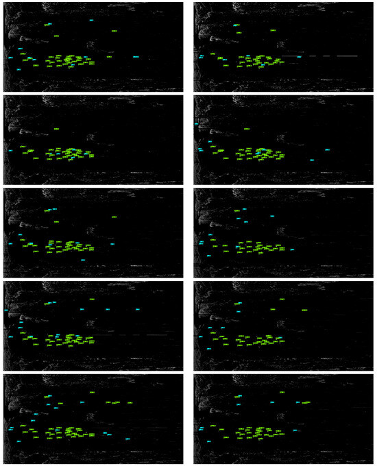
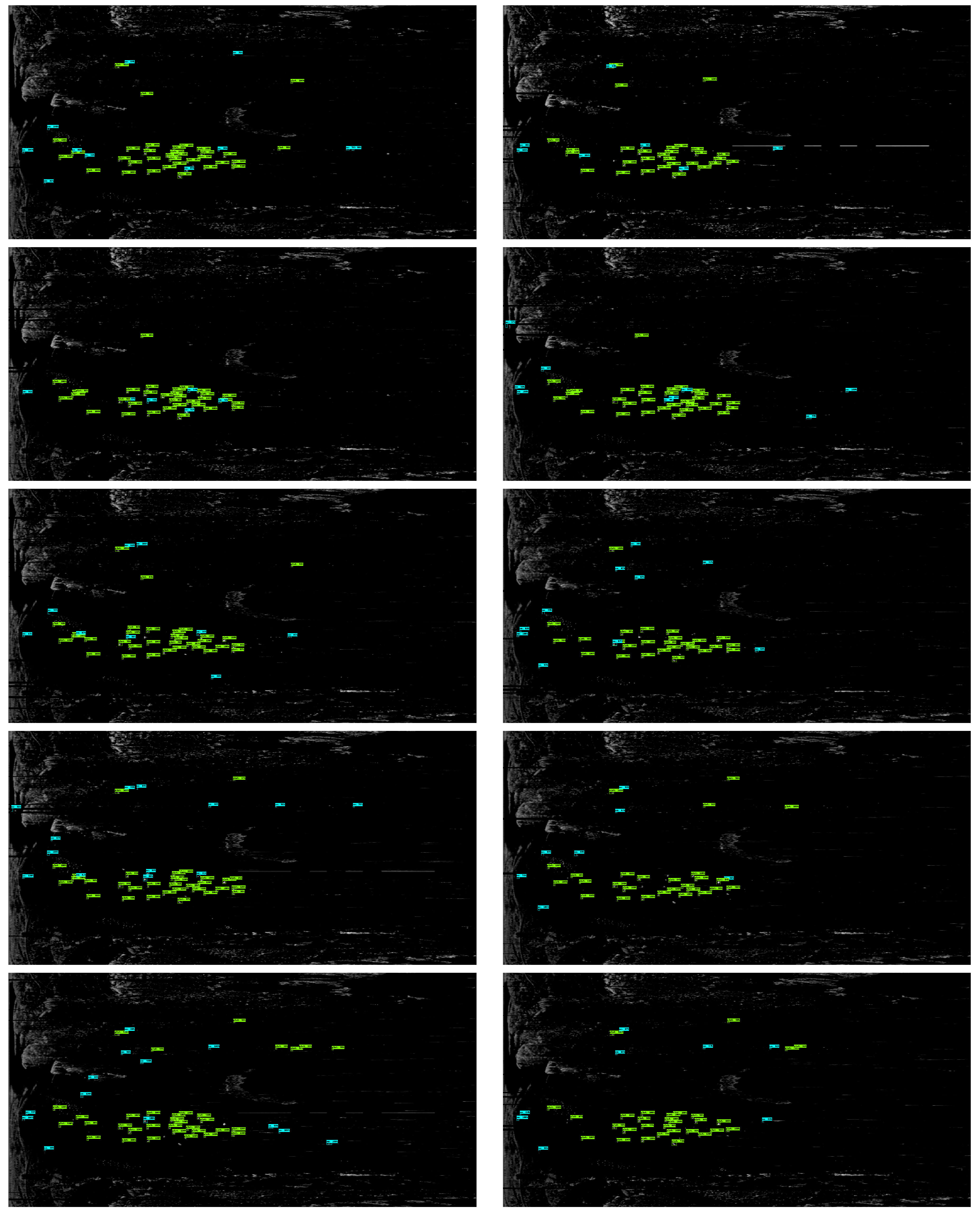
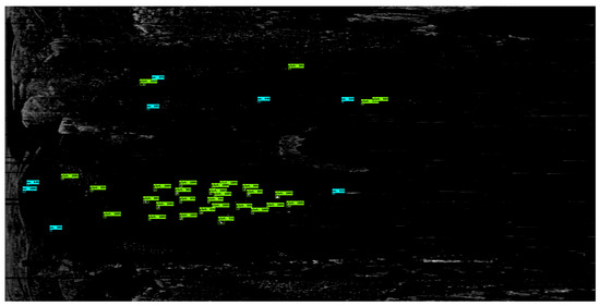
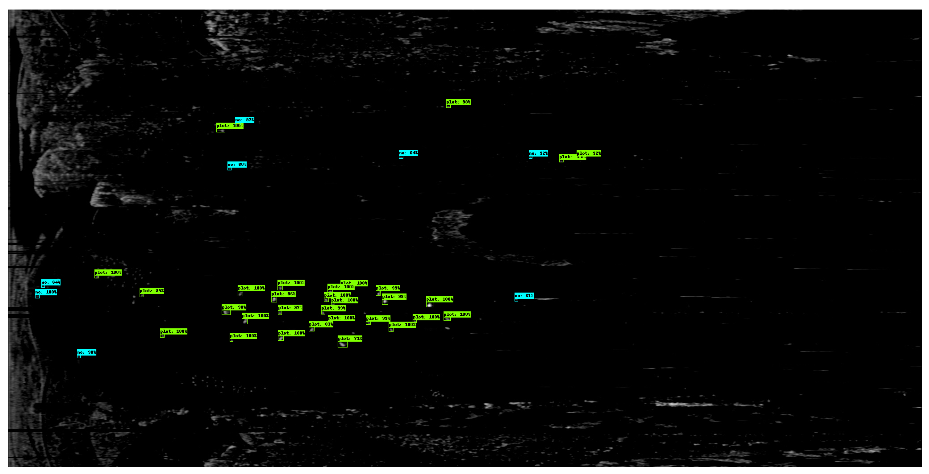
The predictions are represented by bounded boxes containing a class and a confidence score. Two classes are evaluated for the experiments performed: “plot” if it is a marine vessel and “no” if it is not. The predictions yield high confidence scores, which indicate the classification certainty of the models. Figure 15 presents radar images with detected marine vessels using Faster R-CNN object detector trained on 100,000 epochs and using the 10 laps evaluation dataset.

Figure 15. Predictions of marine vessels in the port of Callao, Perú using the Faster R-CNN model (100,000 epochs).

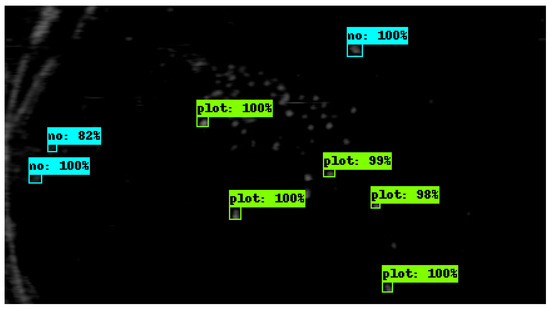
Some predictions obtained with the Faster R-CNN model are shown in Figure 16. Each bounding box includes the label and confidence score. The label corresponds to the class of the object. If the object is a marine vessel, it will have the label “plot”; otherwise, if the detector recognizes that it is not a marine vessel, it will have the label “no”. The confidence score is the measure that the detector assigns according to the certainty of classifying the objects.

Figure 16. Predictions in bounding boxes with the label and the confidence score.

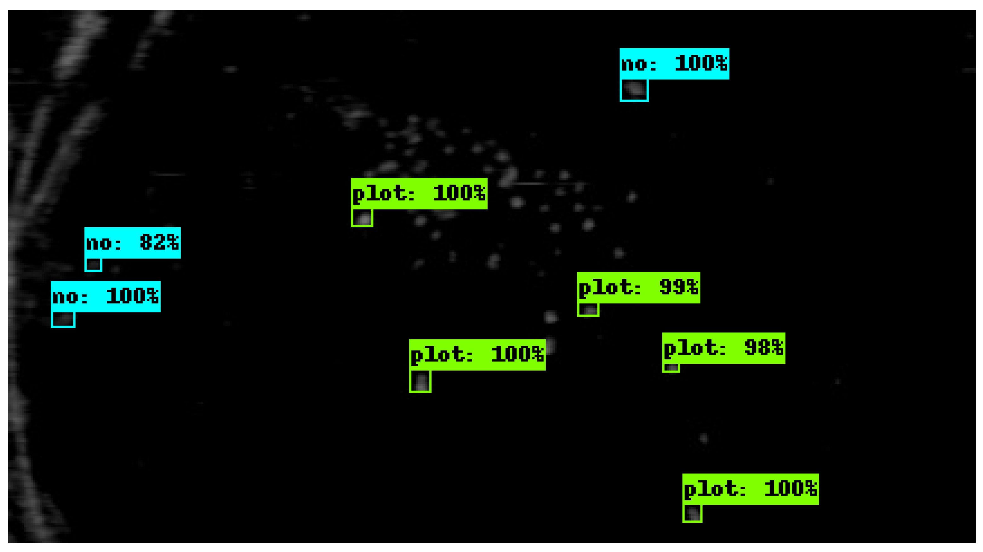
On the other hand, in Figure 17, we can appreciate the degree of certainty or confidence score of the two classes of objects detected, “plot” and “no”, even in the case of the smallest ones. The high degree of confidence obtained is due to a large number of findings that have been learned by the model in the training process.

Figure 17. Confidencescores for both object classes “plot” and “no”.

4.3.4. Processing Time

The total processing time is based on using Google Colab Pro, powered by GPU, Python. The time required by the Faster R-CNN Inception V2 model to obtain the results is calculated. Taking into account only one radar image, with the outputs of graphs, boxes and classes, the measurement obtained is 4.513750 s. The result is shown in (18):

$$T_p=4.513750\mathrm{s}$$

(18)

where:

• Tp: One lap prediction time.
• This is the time required by the model to obtain the predictions, taking into consideration three radar turns, with the outputs of graphs, boxes, and classes being 6.0120687 s. The time required by the algorithm to generate the detected objects from an image is 0.01097893 s. On the other hand, the estimated response time in the tests executed with a single standard processor is equivalent to 4.1 s. Given the technology equipped on the radar vessels, optimizing the estimated response time further is possible.

4.3.5. Future Work

As the Navy provides us with a new batch of radar images in regions of interest, future research is planned to explore single-stage models such as YOLO and SSD. The next experiments should estimate the performance in recovery and precision in scenes of high meteorological complexity and with low-resolution data. Furthermore, experiments should be carried out on high-performance computing platforms.

5. Conclusions

After the analysis of the results, the following statements can be made:

• The detection model yields a cost function value equal to 0.0372, a recall rate of 94.5%, and an accuracy rate of 95.1%.
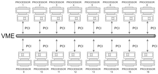
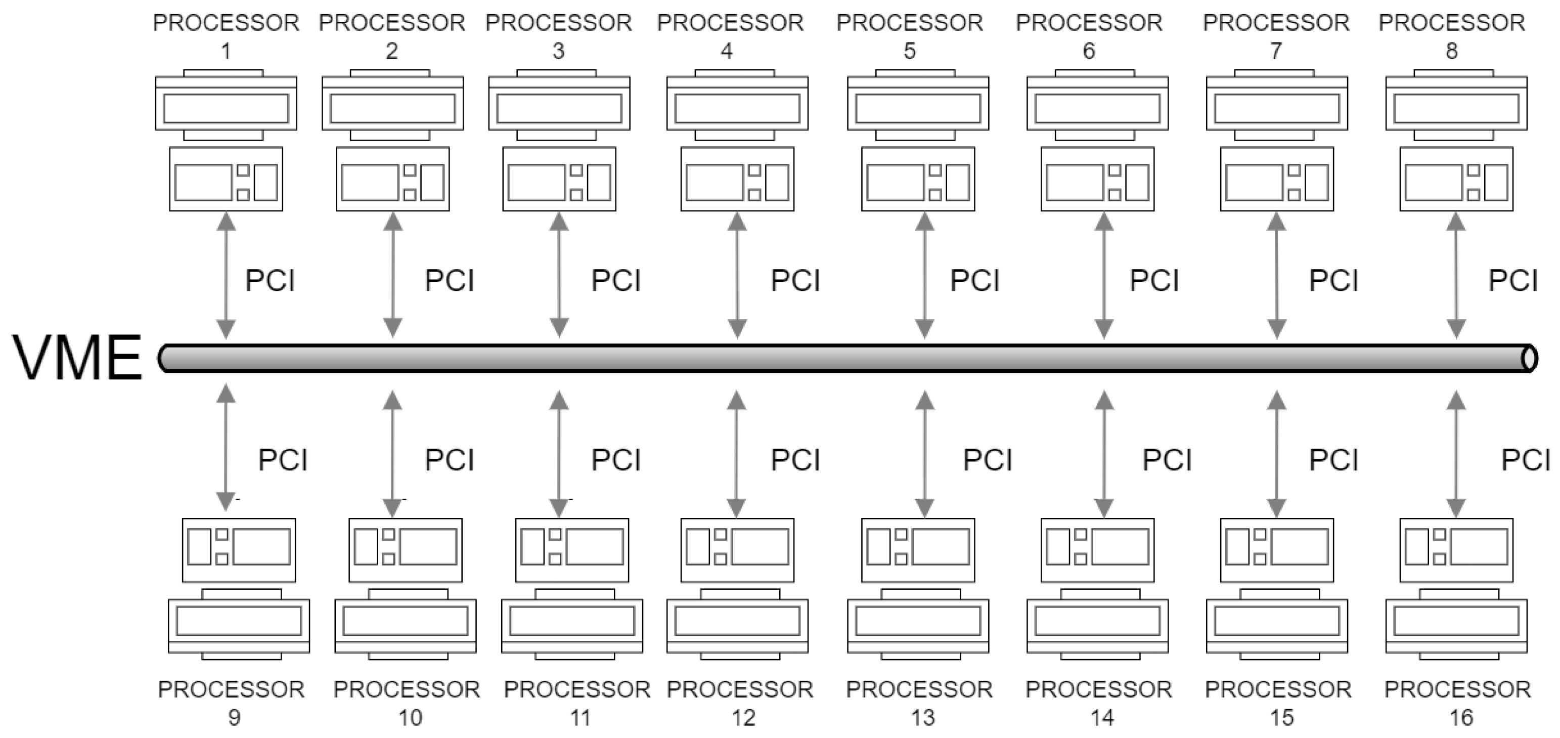
• The detection time is favorable, equivalent to 4.513 s per radar turn. Considering the implementation of the algorithm in an integrated system with a pool of parallel processors, it is feasible to improve the detection time further.
• The modification of weight initialization ($\mu =0$; $\sigma =0.05$) and the ADAM optimizer are the determining hyperparameters in improving the training, and consequently the object detection model. The IoU and batch-size hyperparameters influence but are not decisive in the improvement of the performance of the object detection model.
• The cross-validation method is independent in handling partitions and eliminates bias by randomly selecting samples for training and validation datasets. In addition, it allows the best models to be chosen based on rigorous verification that guarantees their implementation in real projects.
• Automatic cropping makes it easy to obtain more precise cuts of objects quickly. These cuts meet the characteristics of the intensity and dimensions of the objects of interest.
• Displaying objects of interest in three consecutive turns allows for a faster and more reliable labeling process. The developed interface increases the efficiency of object labeling.
• Given the results, with the proposed methodology, it is possible to generate a ship detection model that works well despite the noise and clutter reflected in the radar images. The detection model obtained is valid for use with commercial radar images.
• This work is the beginning of future projects with other deep learning algorithms and using an advanced computing infrastructure.
• The findings may be particularly applicable to other coastal regions, where advanced remote sensing applications have not yet been widely explored.

References

- Kanjir, U.; Greidanus, H.; Oštir, K. Vessel detection and classification from spacebone optical images: A literature survey. Remote Sens. Environ. 2018, 207, 1–26. [Google Scholar] [CrossRef] [Scilit] [PubMed]
- Kingsley, S.; Quegan, S. Understanding Radar Systems; SciTech Publishing Inc.: Mendham, NJ, USA, 1999. [Google Scholar]
- Purizaga-Céspedes, D. Análisis de un Nuevo Filtro de dos Parámetros para Detección de Contactos en imáGenes de Radares Marinos. Bachelor’s Thesis, Universidad de Piura, Piura, Perú, 13 February 2019. Available online: https://hdl.handle.net/11042/3821 (accessed on 24 May 2024).
- Fulvio, G. Chapter 10—Introduction to the Radar Signal Processing Section. In Academic Press Library in Signal Processing; Sidiropoulos, N., Gini, F., Chellappa, R., Theodoridis, S., Eds.; Elsevier: Oxford, UK, 2014; Volume 2, pp. 505–511. [Google Scholar] [CrossRef] [Scilit]
- Javadi, S.; Farina, A. Radar networks: A review of features and challenges. Inf. Fusion 2020, 61, 48–55. [Google Scholar] [CrossRef] [Scilit]
- Meyer, F.; Hinz, S.; Laika, A.; Weihing, D. Performance analysis of the TerraSAR-X Traffic monitoring concept. Photogramm. Remote Sens. 2006, 61, 225–242. [Google Scholar] [CrossRef] [Scilit]
- Petit, M.; Stretta, J.M.; Farrugio, H.; Wadsworth, A. Synthetic aperture radar imaging of sea surface life and fishing activities. IEEE Trans. Geosci. Remote Sens. 1992, 30, 1085–1089. [Google Scholar] [CrossRef] [Scilit]
- Mazur, A.K.; Wahlin, A.K.; Krezel, A. An object-based SAR image iceberg detection algorithm applied to the Amundsen Sea. Remote Sens. Environ. 2017, 189, 67–83. [Google Scholar] [CrossRef] [Scilit]
- Zhang, J.; Xing, M.; Sun, G. A Fast Target Detection Method for SAR Image Based on Electromagnetic Characteristics. In Proceedings of the International SAR Symposium (CISS), Shanghai, China, 10–12 October 2018; pp. 1–3. [Google Scholar] [CrossRef] [Scilit]
- Koyama, C.; Gokon, H.; Koshimura, S. Disaster debris estimation using high-resolution polarimetric stereo-SAR. ISPRS J. Photogramm. Remote Sens. 2016, 120, 84–98. [Google Scholar] [CrossRef] [Scilit]
- An, W.; Xie, C.; Yuan, X. An Improved Iterative Censoring Scheme for CFAR Ship Detection With SAR Imagery. IEEE Trans. Geosci. Remote Sens. 2014, 52, 4585–4595. [Google Scholar] [CrossRef] [Scilit]
- Crisp, D.J. The State-of-the-Art in Ship Detection in Synthetic Aperture Radar Imagery. Defence Science and Technology Organisation Salisbury, Australia. Available online: https://apps.dtic.mil/sti/pdfs/ADA426096.pdf (accessed on 28 May 2024).
- Kang, M.; Leng, X.; Lin, Z.; Ji, K. A modified faster R-CNN based on CFAR algorithm for SAR ship detection. In Proceedings of the International Workshop on Remote Sensing with Intelligent Processing (RSIP), Shanghai, China, 19–21 May 2017; pp. 1–4. [Google Scholar] [CrossRef] [Scilit]
- Wang, Y.; Zhang, Y.; Qu, H.; Tian, Q. Target Detection and Recognition Based on Convolutional Neural Network for SAR Image. In Proceedings of the 2018 11th International Congress on Image and Signal Processing BioMedical Engineering and Informatics (CISP-BMEI), Beijing, China, 13–15 October 2018; pp. 1–5. [Google Scholar] [CrossRef] [Scilit]
- Zhou, S.; Zhou, Z.; Wang, C.; Liang, Y.; Wang, L.; Zhang, J.; Zhang, J.; Lv, C. A User-Centered Framework for Data Privacy Protection Using Large Language Models and Attention Mechanisms. Appl. Sci. 2024, 14, 6824. [Google Scholar] [CrossRef] [Scilit]
- Lee, J.-Y.; Choi, W.-S.; Choi, S.-H. Verification and performance comparison of CNN-based algorithms for two-step helmet-wearing detection. Expert Syst. Appl. 2023, 225, 120096. [Google Scholar] [CrossRef] [Scilit]
- Girshick, R. Fast R-CNN. In Proceedings of the IEEE International Conference on Computer Vision (ICCV), Santiago, Chile, 7–13 December 2015; pp. 1440–1448. [Google Scholar] [CrossRef] [Scilit]
- Ren, S.; He, K.; Girshick, R.; Sun, J. Faster R-CNN: Towards Real-Time Object Detection with Region Proposal Networks. Comput. Vis. Pattern Recognit. 2016, 3, 1137–1149. [Google Scholar] [CrossRef] [Scilit]
- He, K.; Zhang, X.; Ren, S.; Sun, J. Deep Residual Learning for Image Recognition. In Proceedings of the IEEE Conference on Computer Vision and Pattern Recognition (CVPR), Las Vegas, NV, USA, 27–30 June 2016; pp. 770–778. [Google Scholar] [CrossRef] [Scilit]
- Jiao, J.; Zhang, Y.; Sun, H.; Yang, X.; Gao, X.; Hon, W. A Densely Connected End-to-End Neural Network for Multiscale and Multiscene SAR Ship Detection. IEEE Access 2018, 6, 20881–20892. [Google Scholar] [CrossRef] [Scilit]
- Pham, M.; Lefèvre, S. Buried Object Detection from B-Scan Ground Penetrating Radar Data Using Faster-RCNN. In Proceedings of the IEEE International Geoscience and Remote Sensing Symposium (IGARSS), Valencia, Spain, 22–27 July 2018; pp. 6804–6807. [Google Scholar] [CrossRef] [Scilit]
- Sethu Ramasubiramanian, S.; Sivasubramaniyan, S.; Peer Mohamed, M.F. Aggregate Channel Features and Fast Regions CNN Approach for Classification of Ship and Iceberg. Appl. Sci. 2023, 13, 7292. [Google Scholar] [CrossRef] [Scilit]
- Cai, J.; Zhang, L.; Dong, J.; Guo, J.; Wang, Y.; Liao, M. Automatic identification of active landslides over wide areas from time-series InSAR measurements using Faster RCNN. Int. J. Appl. Earth Obs. Geoinf. 2023, 124, 103516. [Google Scholar] [CrossRef] [Scilit]
- Mduduzi, M.; Chunling, T.; Adewale, O. Preprocessed Faster RCNN for Vehicle Detection. In Proceedings of the 2018 International Conference on Intelligent and Innovative Computing Applications (ICONIC), Mon Tresor, Mauritius, 6–7 December 2018; pp. 1–4. [Google Scholar] [CrossRef] [Scilit]
- Gavrilescu, R.; Zet, C.; Foșalău, C. Faster R-CNN: An Approach to Real-Time Object Detection. In Proceedings of the 2018 International Conference and Exposition on Electrical And Power Engineering (EPE), Iasi, Romania, 18–19 October 2018; pp. 165–168. [Google Scholar] [CrossRef] [Scilit]
- Liu, W.; Anguelov, D.; Erhan, D. SSD: Single Shot MultiBox Detector. In Proceedings of the Computer Vision (ECCV), Amsterdam, The Netherlands, 11–14 October 2016; pp. 21–37. [Google Scholar] [CrossRef] [Scilit]
- Redmon, J.; Divvala, S.; Girshick, R.; Farhadi, A. You Only Look Once: Unified, Real-Time Object Detection. In Proceedings of the IEEE Conference on Computer Vision and Pattern Recognition (CVPR), Las Vegas, NV, USA, 27–30 June 2016; pp. 779–788. [Google Scholar] [CrossRef] [Scilit]
- Chen, J.; Shen, Y.; Liang, Y.; Wang, Z.; Zhang, Q. YOLO-SAD: An Efficient SAR Aircraft Detection Network. Appl. Sci. 2024, 14, 3025. [Google Scholar] [CrossRef] [Scilit]
- Guo, J.; Wang, S.; Xu, Q. Saliency Guided DNL-Yolo for Optical Remote Sensing Images for Off-Shore Ship Detection. Appl. Sci. 2022, 12, 2629. [Google Scholar] [CrossRef] [Scilit]
- Liu, J.; Liao, D.; Wang, X.; Li, J.; Yang, B.; Chen, G. LCAS-DetNet: A Ship Target Detection Network for Synthetic Aperture Radar Images. Appl. Sci. 2024, 14, 5322. [Google Scholar] [CrossRef] [Scilit]
- Wang, X.; Hong, W.; Liu, Y.; Hu, D.; Xin, P. SAR Image Aircraft Target Recognition Based on Improved YOLOv5. Appl. Sci. 2023, 13, 6160. [Google Scholar] [CrossRef] [Scilit]
- Yu, J.; Huang, D.; Shi, X.; Li, W.; Wang, X. Real-Time Moving Ship Detection from Low-Resolution Large-Scale Remote Sensing Image Sequence. Appl. Sci. 2023, 13, 2584. [Google Scholar] [CrossRef] [Scilit]
- Botezatu, A.-P.; Burlacu, A.; Orhei, C. A Review of Deep Learning Advancements in Road Analysis for Autonomous Driving. Appl. Sci. 2024, 14, 4705. [Google Scholar] [CrossRef] [Scilit]
- Liang, B.; Wang, Z.; Si, L.; Wei, D.; Gu, J.; Dai, J. A Novel Pressure Relief Hole Recognition Method of Drilling Robot Based on SinGAN and Improved Faster R-CNN. Appl. Sci. 2023, 13, 513. [Google Scholar] [CrossRef] [Scilit]
- Jakubec, M.; Lieskovská, E.; Bučko, B.; Zábovská, K. Comparison of CNN-Based Models for Pothole Detection in Real-World Adverse Conditions: Overview and Evaluation. Appl. Sci. 2023, 13, 5810. [Google Scholar] [CrossRef] [Scilit]
- Altarez, R.D. Faster R–CNN, RetinaNet and Single Shot Detector in different ResNet backbones for marine vessel detection using cross polarization C-band SAR imagery. Remote Sens. Appl. Soc. Environ. 2024, 36, 101297. [Google Scholar] [CrossRef] [Scilit]
- Retallack, A.; Finlayson, G.; Ostendorf, B.; Lewis, M. Using deep learning to detect an indicator arid shrub in ultra-high-resolution UAV imagery. Ecol. Indic. 2022, 145, 109698. [Google Scholar] [CrossRef] [Scilit]
- Li, T.; He, B.; Zheng, Y. Research and Implementation of High Computational Power for Training and Inference of Convolutional Neural Networks. Appl. Sci. 2023, 13, 1003. [Google Scholar] [CrossRef] [Scilit]
- Moreno, V.; Ledezma, A.; Sanchis, A. A Static Images Based-System For Traffic Signs Detection. In Proceedings of the International Conference on Artificial Intelligence and Applications (IASTED), Madrid, Spain, 13–16 February 2006; pp. 445–450. [Google Scholar]
- Moreno, V.; Génova, G.; Alejandres, M.; Fraga, A. Automatic Classification of Web Images as UML Static Diagrams Using Machine Learning Techniques. Appl. Sci. 2020, 10, 2406. [Google Scholar] [CrossRef] [Scilit]
- Gonzales-Martínez, R.; Machacuay, J.; Rotta, P.; Chinguel, C. Real-Time Detection Method of Persistent Objects in Radar Imagery with Deep Learning. In Proceedings of the IEEE Engineering International Research Conference (EIRCON), Lima, Peru, 21–23 October 2020; pp. 1–4. [Google Scholar] [CrossRef] [Scilit]
- Gonzales-Martínez, R.; Machacuay, J.; Rotta, P.; Chinguel, C. Hyperparameters Tuning of Faster R-CNN Deep Learning Transfer for Persistent Object Detection in Radar Images. IEEE Lat. Am. Trans. 2022, 20, 677–685. [Google Scholar] [CrossRef] [Scilit]
- LabelImg. HumanSignal labelImg. Available online: https://github.com/HumanSignal/labelImg (accessed on 4 September 2024).
- Rubin, B.; Sathiesh, K. Efficient inception V2 based deep convolutional neural network for real-time hand action recognition. IET Image Process. 2020, 14, 688–696. [Google Scholar] [CrossRef] [Scilit]
- Vijiyakumar, K.; Govindasamy, V.; Akila, V. An effective object detection and tracking using automated image annotation with inception based faster R-CNN model. Int. J. Cogn. Comput. Eng. 2024, 5, 343–356. [Google Scholar] [CrossRef] [Scilit]
- Siddiqi, M.D.; Jiang, B.; Asadi, R.; Regan, A. Hyperparameter Tuning to Optimize Implementations of Denoising Autoencoders for Imputation of Missing Spatio-temporal Data. Procedia Comput. Sci. 2021, 184, 107–114. [Google Scholar] [CrossRef] [Scilit]
- Lee, W.Y.; Park, S.M.; Sim, K.B. Optimal hyperparameter tuning of convolutional neural networks based on the parameter-setting-free harmony search algorithm. Optik 2018, 172, 359–367. [Google Scholar] [CrossRef] [Scilit]
- Diederik, P.K.; Ba, J. Adam: A Method for Stochastic Optimization. In Proceedings of the 3rd International Conference for Learning Representations, San Diego, CA, USA, 7–9 May 2015. [Google Scholar] [CrossRef] [Scilit]
- Schöller, F.; Plenge-Feidenhans’l, M.; Stets, J.; Blanke, M. Assessing Deep-learning Methods for Object Detection at Sea from LWIR Images. IFAC-PapersOnLine 2019, 52, 64–71. [Google Scholar] [CrossRef] [Scilit]
- Zhang, T.; Zhang, X. High-Speed Ship Detection in SAR Images Based on a Grid Convolutional Neural Network. GPU Comput. Geosci. Remote Sens. 2019, 11, 1206. [Google Scholar] [CrossRef] [Scilit]
- Yuan, Y.; Rosasco, L.; Caponnetto, A. On Early Stopping in Gradient Descent Learning. Constr. Approx. 2007, 26, 289–315. [Google Scholar] [CrossRef] [Scilit]
- Wang, Y.; Zhang, H.; Zhang, G. cPSO-CNN: An efficient PSO-based algorithm for fine-tuning hyper-parameters of convolutional neural networks. Swarm Evol. Comput. 2019, 49, 114–123. [Google Scholar] [CrossRef] [Scilit]
- Dewa, C.K. Suitable CNN Weight Initialization and Activation Function for Javanese Vowels Classification. Procedia Comput. Sci. 2018, 144, 124–132. [Google Scholar] [CrossRef] [Scilit]
- Hastie, T.; Tibshirani, R.; Friedman, J. The Elements of Statistical Learning: Data Mining, Inference and Prediction, 2nd ed.; Springer: New York, NY, USA, 2009; pp. 389–415. [Google Scholar]
- Paneiro, G.; Rafael, M. Artificial neural network with a cross-validation approach to blast-induced ground vibration propagation modeling. Undergr. Space 2021, 6, 281–289. [Google Scholar] [CrossRef] [Scilit]
- Valente, G.; Lage Castellanos, A.; Hausfeld, L.; De Martino, F.; Formisano, E. Cross-validation and permutations in MVPA: Validity of permutation strategies and power of cross-validation schemes. NeuroImage 2021, 238, 118145. [Google Scholar] [CrossRef] [Scilit] [PubMed]
- Kerbaa, T.H.; Mezache, A.; Oudira, H. Model Selection of Sea CLutter Using Cross Validation Method. Procedia Comput. Sci. 2019, 158, 394–400. [Google Scholar] [CrossRef] [Scilit]
- Gonzales-Martínez, R.; Machacuay, J.; Rotta, P.; Chinguel, C. Faster R-CNN with a cross-validation approach to object detection in radar images. In Proceedings of the 2021 IEEE International Conference on Aerospace and Signal Processing (INCAS), Lima, Peru, 28–30 November 2021; pp. 1–4. [Google Scholar] [CrossRef] [Scilit]
- Padilla, R.; Passos, W.; Dias, T.; Netto, S.; da Silva, E. A Comparative Analysis of Object Detection Metrics with a Companion Open-Source Toolkit. Deep Learn. Based Obj. Detect. 2021, 10, 279. [Google Scholar] [CrossRef] [Scilit]
- Li, Y.; Deng, J.; Wu, Q.; Wang, Y. Eye-Tracking Signals Based Affective Classification Employing Deep Gradient Convolutional Neural Networks. Int. J. Interact. Multimed. Artif. Intell. 2021, 7, 34–43. [Google Scholar] [CrossRef] [Scilit]
Disclaimer/Publisher’s Note: The statements, opinions and data contained in all publications are solely those of the individual author(s) and contributor(s) and not of MDPI and/or the editor(s). MDPI and/or the editor(s) disclaim responsibility for any injury to people or property resulting from any ideas, methods, instructions or products referred to in the content. |
© 2024 by the authors. Licensee MDPI, Basel, Switzerland. This article is an open access article distributed under the terms and conditions of the Creative Commons Attribution (CC BY) license (https://creativecommons.org/licenses/by/4.0/).