PESO: A Seq2Seq-Based Vessel Trajectory Prediction Method with Parallel Encoders and Ship-Oriented Decoder

Abstract

Vessel trajectory prediction supports navigation services and collision detection. To maintain safety and efficiency in maritime transportation, vessel trajectory prediction is always an important topic. By using automatic identification system (AIS) data and deep learning methods, the task of vessel trajectory prediction has made significant progress. However, this task is still full of challenges due to the complexity of historical information dependencies and the strong influence of spatial correlations. In this paper, we introduce a novel deep learning model, PESO, based on the structure of Seq2Seq, consisting of Parallel Encoders and a Ship-Oriented Decoder. The Parallel Encoders, including the Location Encoder and the Sailing Status Encoder are designed to integrate more information into feature representation. The Ship-Oriented Decoder is targeted to utilize the Semantic Location Vector (SLV) to guide the prediction, which better represents the spatial correlation of historical track points. In order to verify the efficiency and efficacy of PESO, we conducted comparative experiments with several baseline models. The experimental results demonstrate that PESO is superior to them both quantitatively and qualitatively.

1. Introduction

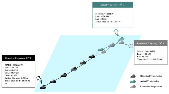
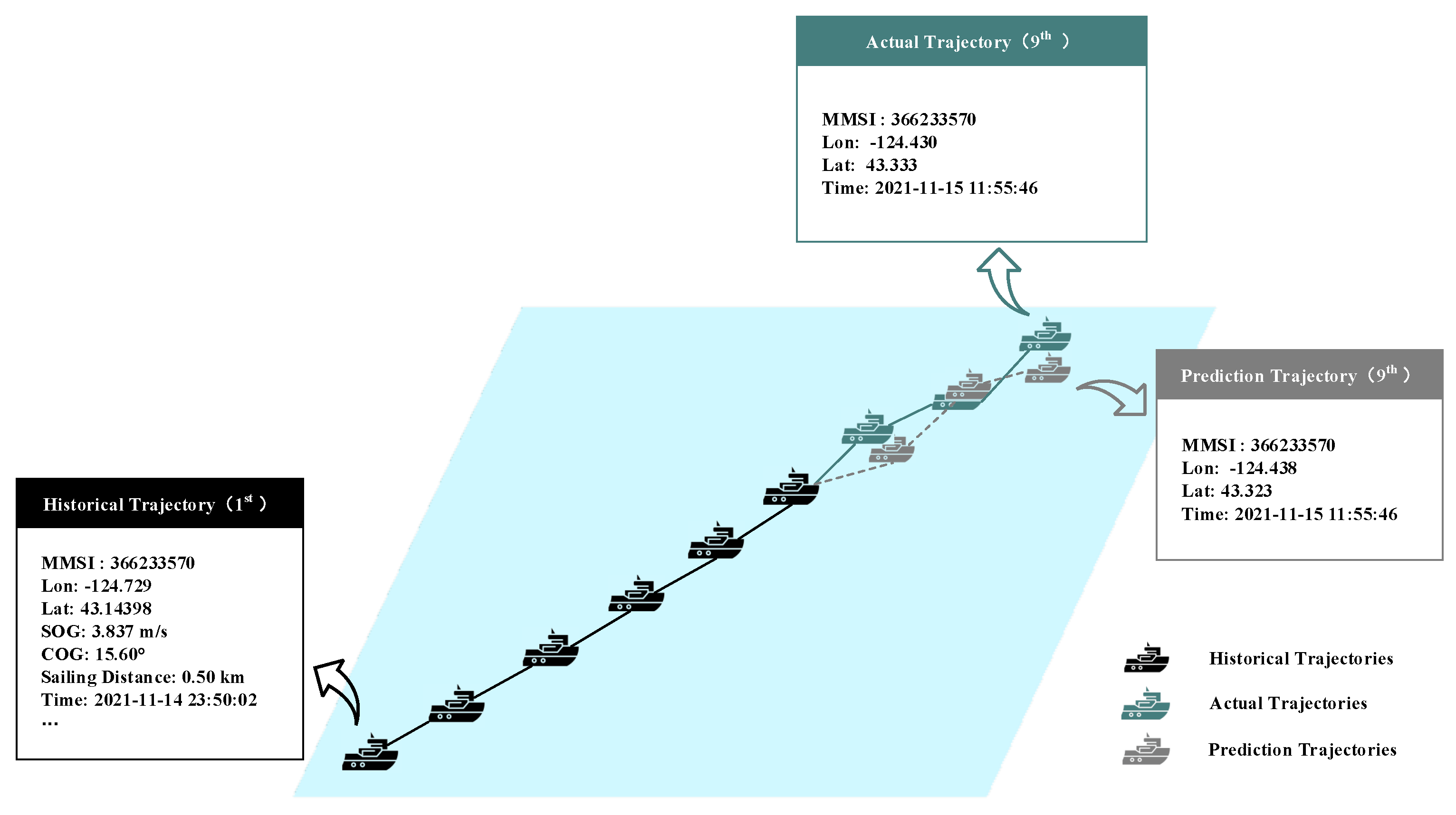
In the past few decades, maritime transportation has increased dramatically with the constant growth in global trade. It is essential to ensure the the safety and efficiency of the vessels while sailing. Predicting the next trajectories of a vessel by using automatic identification system (AIS) data can prevent the incorrect navigation and collisions, avoiding human casualties, property loss, and environmental pollution. Specifically, vessel trajectory prediction is a task to predict the following trajectory locations with several historical track points. Figure 1 shows an example of vessel trajectory prediction. Traditional vessel trajectory prediction studies are mostly based on simulation and statistical methods, such as stochastic processes. These methods can predict with moderate accuracy but are limited by computational consumption and coarse semantic information. With the successful application of deep learning in many other fields, researchers have begun to utilize deep learning to predict vessel trajectories.

Figure 1. An example of vessel trajectory prediction. The black ships denote the historical AIS trajectories. The grey ships denote the prediction results, while the blue ships denote the actual trajectories.

Deep learning has been widely applied in many scenarios and has achieved remarkable progress. Numerous studies have proposed deep learning methods to predict vessel trajectories in which the prediction process is always considered a time-series regression task. Some of them use a single recurrent neural network that takes the spatiotemporal feature information of the track points as inputs and outputs the position information of the predicted trajectories. In contrast, other studies adopt a Seq2Seq structure consisting of an encoder and a decoder. The input feature information is embedded by the encoder to generate high-dimensional representations and transmitted to the decoder for prediction. These methods obtain more semantic level information than traditional methods, enabling more accurate predictions. However, due to the complexity of historical information dependencies and the strong influence of spatial correlations, accurate prediction remains a challenge. Specifically, the prediction of the track point locations during the following parts of a voyage often relies on historical trajectory information and is also influenced by the historical spatial position of the ship. As a result, it is crucial to make the network capture richer features from historical information and better represent the spatial correlation of historical track points.

More recently, relying on the technology support from trajectory prediction methods, most commercial systems can detect collisions and provide navigation services. A prediction with significant deviation will influence the efficiency and safety of the vessels. Several state-of-the-art methods have been proposed to address the problem. For example, ref. [1] applies uncertainty quantification in their works, and [2] proposes a network optimized by a genetic algorithm. Unlike these methods, we propose a novel deep learning model, PESO, for vessel trajectory prediction, consisting of the Parallel Encoders and the Ship-Oriented Decoder. The Parallel Encoders are designed to integrate more feature information into deep representation by using different encoders to obtain multiple features, which include the Location Encoder and the Sailing Status Encoder. Processing different types of features with the same encodery will produce more noise and affect the accuracy of prediction. The Location Encoder embeds the longitude and latitude into representations, while the Sailing Status Encoder encodes the course, speed, and sailing distance. The Parallel Encoders embed different types of features simultaneously and enrich feature representation, avoiding the noise inside the features. The Ship-Oriented Decoder is targeted to utilize the Semantic Location Vector (SLV) of each ship to guide the prediction process, which better represents the spatial correlation of historical track points. The SLV is the semantic representation of each vessel, which contains spatial information related to the historical track points of the vessel. After dividing the map into several grids and obtaining the semantic vector of each grid by the algorithm of continuous bag-of-words (CBOW) [3], SLV is generated by the mean of the semantic vectors of all track points of each ship. The Ship-Oriented Decoder uses the combination of feature representations from the Parallel Encoders and SLV as input and outputs the predicted longitude and latitude.

To sum up, the main contributions of this paper can be summarized as follows:

• We propose a novel deep learning model, PESO, based on a Seq2Seq network for vessel trajectory prediction, which aims to capture richer features from previous information and better represent the spatial correlation of historical trajectory points.
• We develop Parallel Encoders, including Location Encoder and the Sailing Status Encoder, to capture more information from longitude, latitude, COG, SOG, and sailing distance.
• We develop the Ship-Oriented Decoder and the Semantic Location Vector (SLV). The Ship-Oriented Decoder can utilize the SLV to generate accurate prediction results, which better represent the spatial correlation of historical track points.
• We implement comparative experiments with several baseline models. The experimental results show that our model is superior to them both quantitatively and qualitatively.

2. Related Works

2.1. Seq2Seq Model

The Seq2Seq model is a widely used structure in deep learning, which was proposed in [4] for machine translation in 2014. A Seq2Seq model includes an encoder and a decoder. The encoder embeds the input information and generates high-dimensional representation features. The decoder embeds the representation features from the encoder and outputs the results.

The Seq2Seq model is widely used in regression tasks. Scholars in [5] proposed a Seq2Seq architecture for time-series forecasting which is used as a general purpose forecasting method. Ref. [6] proposes an appliance-level load forecasting model of long short-term memory (LSTM)-based Seq2Seq learning for residential homes in the field of load forecasting. Ref. [7] uses the extended deep Seq2Seq long short-term memory regression (STSR-LSTM) model for wind power forecasting. A nonintrusive load monitoring model is proposed by [8], which is targeted to address the problems of low accuracy and high misjudgment rate of disaggregated power value. An LSTM-based Seq2Seq model is proposed to forecast with multi-step and make the best use of different input variables in the work of [9]. Ref. [10] proposes a novel model for energy load forecasting by utilizing recurrent neural networks (RNN) to obtain time dependencies. A Seq2Seq model with attention and monotonicity loss (SMAML) is introduced to simultaneously predict and monitor the tool wear in the work of [11]. A novel Seq2Seq rainfall–runoff model is proposed in [12]’s work based on LSTM. Ref. [13] proposes a system to predict the future values of a stock using bi-directional long short-term memory(BiLSTM)-based Seq2Seq modelling. Ref. [14] proposes a novel method foraue prediction based on a Seq2Seq recurrent neural network. Ref. [15] develops a Seq2Seq learning model for multistep-ahead prediction on soil temperature and moisture. Ref. [16] presents a deep neural network architecture that aims to use it in time-series weather prediction. Ref. [17] proposes four Seq2Seq models to improve runoff prediction performance in ungauged basins.

2.2. Vessel Trajectory Prediction

Vessel trajectory prediction methods based on deep learning are developing rapidly. Most deep learning models adopt RNN structures. For example, some models are based on LSTM [18] or gate recurrent unit (GRU) [4]. Ref. [19] proposes an LSTM model for vessel trajectory prediction combined with the sequence prediction method. Furthermore, ref. [20] explores BiLSTM, which can enhance more relevance between historical and future time-series data compared to single LSTM and improve the accuracy. To focus on the different sections of hidden features of the BiLSTM network, ref. [21] introduces the attention mechanism into the task. In the work of [22], researchers train a single LSTM model for each type of vessel since the type of a vessel may influence its movement characteristics. Using automatic identification system (AIS) data, ref. [23] investigates a novel approach based on variational LSTM to predict the trajectory of a vessel. Ref. [24] selects a bi-directional gate recurrent unit (BiGRU) network with less trainable parameters for estimation. Others are trying to utilize the Seq2Seq frameworks to solve the task. To address the problem of trajectory prediction with uncertainty quantification, ref. [25] proposes an attention-based recurrent encoder–decoder model. Ref. [26] presents a method based on the Seq2Seq model which uses a spatial grid for trajectory prediction. In the study of [27], a neural Seq2Seq model is proposed, which is based on the LSTM encoder–decoder architecture to capture long-term temporal dependencies of AIS data effectively. Ref. [28] incorporates both spatial and temporal attention mechanisms and proposes a novel attention-based LSTM encoder–decoder method on the structure of [27]. Ref. [29] proposes a Seq2Seq framework based on GRU for short-term prediction. The researchers in [30] introduce a recurrent encoder–decoder model to address the problem of the presence of complex mobility patterns. Ref. [31] proposes a novel vessel trajectory prediction model, which is based on the integrated model of LSTM auto-encode, attention mechanism, and bi-directional LSTM (AABiL) structure. The researchers in [32] introduce generative adversarial networks [33] into trajectory prediction, where they use an LSTM Seq2Seq model as the generator and a naive LSTM as the discriminator. Ref. [34] formulates a transformer-based model for vessel trajectory prediction which embeds the inputs into higher-dimensional vectors.

We are committed to a long-term prediction model. The current short-term prediction models focus on the status of ships in a short period, and the time granularity is less than 20 min. The long-term prediction model is used for long-term prediction, which is more helpful for collision detection and risk warning in practice.

3. Proposed Method

In this section, we will introduce our proposed method in three aspects. First of all, we will discuss relative definitions and statements of PESO. Secondly, we will introduce the data preprocessing process in our model. Finally, we will make a comprehensive description of our proposed model, PESO, including the Semantic Location Vector, the Parallel Encoders, the Ship-Oriented Decoder, and the objective function. Note that we focus on predicting the sequence of five consecutive track points by using a sequence of the previous ten track points in this paper.

3.1. Definitions and Problem Statements

The aim of PESO is to predict the vessel trajectory based on AIS data. In order to express the related operations in our method more clearly, we will use the following definitions:

Definition 1.

(Vessel trajectory): A track point is defined as a tuple $x_t$ = ($LO{N}_t,LA{T}_t,SO{G}_t,CO{G}_t,$ $DI{S}_t$) at the time of t in which $x_t$ is composed of longitude $LO{N}_t$, latitude $LA{T}_t$, speed $SO{G}_t$, course $CO{G}_t$, and sailing distance $DI{S}_t$ respectively, and a vessel trajectory X = ($x_{t_0},x_{t_1},\dots ,x_{t_n}$) is defined as a sequence of these points arranged in chronological order where {$t_i,i=0,1,2,\dots ,n$} is a set of timestamps.

Definition 2.

(Position sequence): Consider the location of a vessel only. A position of a ship is defined as a tuple $y_i$ = ($LO{N}_i,LA{T}_i$) at the time of i, and a position sequence of a ship is defined as Y = ($y1,y2,\dots ,yt$) at a timestamps ($1,2,\dots ,t$).

Definition 3.

(Vessel trajectory prediction): Given an observed trajectory X = ($x_1,x_2,\dots ,x_t$) at timestamp ($1,2,3,\dots ,t$), the scenario aims to predict the following position state of the vessel Y = ($y_{t+1},y_{t+2},\dots ,y_{t+k}$) at the following timestamps ($t+1,t+2,\dots ,t+k$).

3.2. Data Preprocessing

We download the raw AIS data for the southeast and southwest coastal waters of the United States in the whole year of 2021 on the website (https://marinecadastre.gov/accessais/ (accessed on 31 December 2021). We conduct comprehensive data preprocessing on the raw data and use it to train, validate, and test the model. Specifically, raw AIS data have the issues of data errors and high latency, and the targets are to denoise and cut the track points with equal time intervals, which can improve the performance of deep learning models significantly.

The main process includes six steps. Firstly, we separate the trajectory data of different ships by maritime mobile service identify (MMSI) number, the unique ID of a vessel, and sort the track points of each vessel by timestamps. Secondly, we delete the duplicate and anomalous data. After that, we set the time interval of trajectory points to 30 min and perform cubic spline interpolation [35] on possible track points. Fourthly, we cut the trajectory into different segments by judging that the distance between three consecutive trajectory points is less than 100 m. Fifthly, we calculate the value of speed and course for new interpolated trajectory points. Finally, we normalize longitude, latitude, speed, course, and sailing distance by the Min–Max Normalization method.

3.3. PESO

The Seq2Seq model has been widely used in regression tasks. A Seq2Seq model consists of an encoder and a decoder. The encoder embeds the input sequence as semantic representations, and the decoder maps the representation to the output. $Enc$ and $Dec$ denote the encoder and decoder, respectively, while $X_{inp}$ and $Y_{oup}$ are the input and output of the Seq2Seq model, respectively. C is the semantic representation generated by the encoder.

$$\begin{array}{c}C=Enc\left(X_{inp}\right)\\ Y_{oup}=Dec\left(C\right)\end{array}$$

(1)

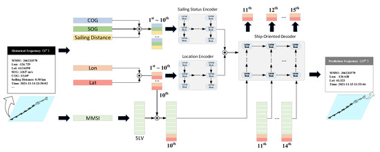
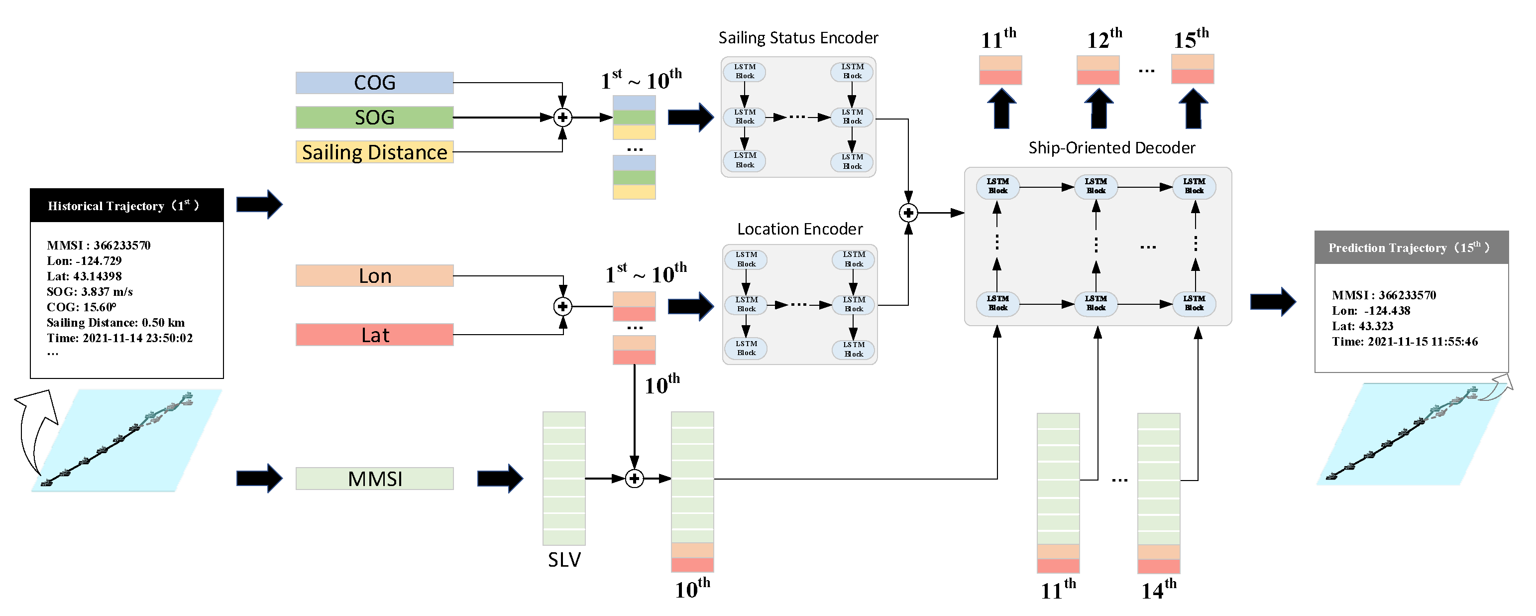
We propose a novel trajectory prediction model, PESO, based on the Seq2Seq structure with Parallel Encoders and a Ship-Oriented Decoder. PESO is composed of three parts as Figure 2 shows: the Semantic Location Vector, the Parallel Encoders, and the Ship-Oriented Decoder. The Semantic Location Vector is the semantic representation of each ship on the grids, containing spatial information related to the ship’s historical track points. The Parallel Encoders are designed to capture more feature information using different encoders to obtain multiple feature representations. The Ship-Oriented Decoder is targeted to utilize the Semantic Location Vector (SLV) of each ship to guide the prediction.

Figure 2. PESO is composed of a Semantic Location Vector (SLV), Parallel Encoders, and a Ship-Oriented Decoder. The SLV of a particular ship represents the spatial correlation of its trajectories. The Parallel Encoders are designed to capture more features by using two different encoders, which include the Location Encoder and the Sailing Status Encoder. The Ship-Oriented Decoder is designed to utilize the SLV to guide the decoding process.

3.3.1. Semantic Location Vector

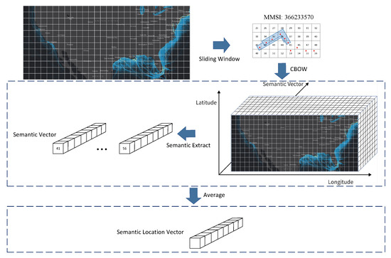
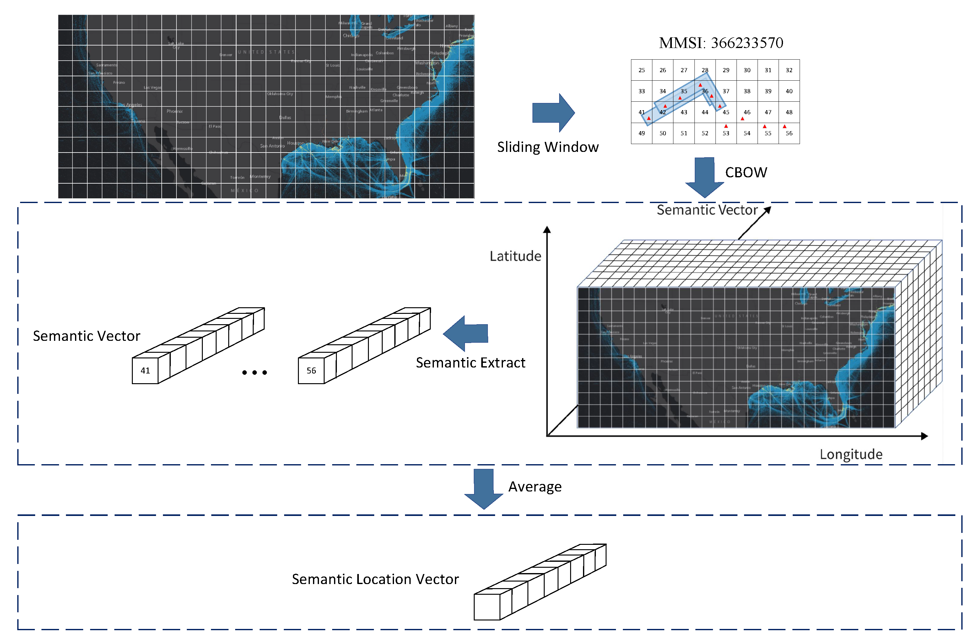
It is insufficient to consider only the previous ten track points before the current timestamp as spatial correlation. In our model, we consider the spatial correlation between the future trajectory points and the observable historical trajectory points of a vessel, which can better simulate the navigation process and obtain satisfactory prediction results. Figure 3 shows the workflow of obtaining the Semantic Location Vector. Technically, we mesh the areas involved in the trajectory points of the vessel in the training set, with 0.1 latitude and 0.1 longitude as a grid. We segment the trajectory according to the mechanism of sliding windows into several groups. Each group consists of 5 trajectory points $(p_1$, $p_2$, $p_3$, $p_4$, $p_5)$, and we calculate the corresponding grid serial number $(g_1$, $g_2$, $g_3$, $g_4$, $g_5)$ for each group. CBOW is an algorithm converting words into vectors in natural language processing, which predicts the central word from surrounding words. PESO mainly utilizes the CBOW model to map the grids to 8-dimensional vectors with spatial location semantics. The CBOW model consists of an embedding layer $Embedding$ and two linear layers $Linea{r}_{cbow1}$ and $Linea{r}_{cbow2}$. The embedding layer aims to encode the grid number into an 8-dimensional vector, and the loss function is the cross-entropy function. The training process can be summarized as follows:

$$\begin{array}{cc}\hfill in{p}_{cbow}& =(g_1;g_2;g_4;g_5)\hfill \\ \hfill em{b}_{cbow}& =Embedding\left(in{p}_{cbow}\right)\hfill \\ \hfill fe{a}_1& =Relu\left(Linea{r}_{cbow}^1\left(em{b}_{cbow}\right)\right)\hfill \\ \hfill ou{t}_{cbow}& =LogSoftmax(\left(Linea{r}_{cbow}^2\left(fe{a}_1\right)\right)\hfill \end{array}$$

(2)

where $ou{t}_{cbow}$ is the output of CBOW, and $em{b}_{cbow}$ is the semantic vector of the grid with number of $g_3$. $Relu$ and $LogSoftmax$ denote nonlinear activation functions, and the objective function is:

$$\begin{array}{c}\hfill objectiv{e}_{cbow}=CrossEntropy(ou{t}_{cbow},g_3)\end{array}$$

(3)

Figure 3. Workflow for obtaining the Semantic Location Vector. First, we divide the sea areas of our dataset with 0.1 latitude and 0.1 longitude as a grid. Then, we use sliding window to conduct a training set of a CBOW model. After training, this model can map every grid to an 8-dimensional semantic vector. Finally, after collecting all the grids corresponding to a vessel, we average the semantic vectors of these grids to obtain the Semantic Location Vector (SLV).

When the training process of the CBOW model is completed, we will obtain the semantic vectors corresponding to each grid on the map. Precisely, for each ship in the training set, we will obtain the semantic vectors corresponding to all the track points. Furthermore, we average the semantic vectors of all the track points of a ship to obtain the Semantic Location Vector of the ship. Take a vessel of ID i as an example, and suppose there are k track points in total associated with the vessel. The formula can be computed as:

$$\begin{array}{c}\hfill SL{V}_i=Avg(sl{v}_1^i,sl{v}_2^i,sl{v}_3^i,\dots sl{v}_k^i)\end{array}$$

(4)

3.3.2. Parallel Encoders

Recurrent neural networks are widely utilized in time-series problems, especially when the variant LSTM appears. LSTM is an extended variant of RNNs with a forgetting gate and a memory cell. The network design ensures that LSTM is capable of learning the long-term temporal dependencies on those time-series data. Normally, an LSTM network comprises several sections, including input data, hidden state, cell memory, model layer, and so on. The detailed calculation process of LSTM can be represented by the following formula, where $f_t$, $i_t$, $C_t$, and $h_t$ denote the forget gate, input gate, cell memory, and hidden state at the time of t, and $x_t$, $C_{t-1}$, and $h_{t-1}$ are the input data at the time of $t-1$; $\sigma$ is the sigmoid function, and $tanh$ is the tanh activation function, while W and b are the learnable parameters in LSTM. ∗ denotes an element-wise product.

$$\begin{array}{cc}\hfill cc{f}_t& =\sigma (W_f·(h_{t-1};x_t)+b_f)\hfill \\ \hfill i_t& =\sigma (W_i·(h_{t-1};x_t)+b_i)\hfill \\ \hfill {\widehat{C}}_t& =tanh(W_C·(h_{t-1};x_t)+b_C)\hfill \\ \hfill C_t& =f_t\ast C_{t-1}+i_t\ast {\widehat{C}}_t\hfill \\ \hfill o_t& =\sigma (W_o·(h_{t-1};x_t)+b_o)\hfill \\ \hfill h_t& =o_t\ast tanh\left(C_t\right)\hfill \end{array}$$

(5)

The Parallel Encoders are targeted to make the networks capture more feature information by using different encoders, obtaining multiple feature representations. The Parallel Encoders embed different types of features at the same time, avoiding the noise inside the features when only an encoder is used, and enrich feature representations. Both encoders in PESO adopt the network of LSTM with five layers. One is the Location Encoder which is specifically designed to embed the position into high-dimensional features. The other is the Sailing Status Encoder, which deals with status information, such as speed, course, and sailing distance.

The Location Encoder $E_{loc}$ sends the input data consisting of normalized longitude and latitude into the network and outputs the hidden state $h_{loc}$ and cell memory $c_{loc}$ which contain the location feature. The input sequence of the Location Encoder is $X_{loc}=(lo{c}_1;lo{c}_2;\dots ;lo{c}_{10})$, where $lo{c}_i=(lo{n}_i;la{t}_i)$, $i=1,2,\dots 10$, and $X_{loc}\in {\mathbb{R}}^{10\times 2}$.

$$\begin{array}{c}\hfill h_{loc},c_{loc}=E_{loc}\left(X_{loc}\right)\end{array}$$

(6)

The Sailing Status Encoder $E_{sail}$ uses the speed, course, and sailing distance of the vessel as inputs to the network, outputting hidden state $h_{sail}$ and cell memory $c_{sail}$. Similarly, the input sequence of the Sailing Status Encoder is $X_{sail}=(sai{l}_1;sai{l}_2;\dots ;sai{l}_{10})$, where $sai{l}_i=(co{g}_i;so{g}_i;di{s}_i)$, $i=1,2,\dots 10$ and $X_{sail}\in {\mathbb{R}}^{10\times 3}$. $h_{sail}$, and $c_{sail}$ represent the sailing status information of the ship.

$$\begin{array}{c}\hfill h_{sail},c_{sail}=E_{sail}\left(X_{sail}\right)\end{array}$$

(7)

Note that $h_{loc}$, $c_{loc}$, $h_{sail}$, and $c_{sail}\in {\mathbb{R}}^{layers\times batchsize\times hidden}$. Finally, for better fusion of features, we add the hidden states and the cell memories of the two encoders to obtain the final result:

$$\begin{array}{cc}\hfill h_{enc}& =h_{loc}+h_{sail}\hfill \\ \hfill c_{enc}& =c_{loc}+c_{sail}\hfill \end{array}$$

(8)

3.3.3. Ship-Oriented Decoder

As described above, the Semantic Location Vector is the spatial semantic representation of each ship’s historical trajectories. The Ship-Oriented Decoder is designed to utilize the Semantic Location Vector (SLV) of each ship to guide the prediction of the vessel trajectory. With this approach, we better express the spatial correlation of the predicted trajectories of each ship. The Ship-Oriented Decoder is composed of five LSTM layers. The decoder takes SLV, input track points, $h_{enc}$, and $c_{enc}$, generated by the Parallel Encoders as inputs. Finally, the model outputs the predicted coordinate sequence of five track points. In this paper, we focus on predicting the longitude and latitude of the following 5 track points by using the previous 10. Technically, the predicting process during training is different from the testing and validation period.

The model based on Seq2Seq structure is able to predict multiple points instead of using a sliding window mechanism. When predicting $y_t$ at the time of t during training, we use $y_{t-1}$ as the coordinate of the nearest trajectory point, where $y_t$ = ($lo{n}_t,la{t}_t$) and $dec$ denote the mapping function of the Ship-Oriented Decoder.

$$\begin{array}{c}\hfill {\widehat{y}}_{t-1}=dec(y_{t-1},SLV,h_{enc},c_{enc})\end{array}$$

(9)

Specifically, the detailed process in Equation (9) is displayed as follows:

$$\begin{array}{cc}\hfill T{r}_t& =concat(y_{t-1},SLV)\hfill \\ \hfill {\widehat{Tr}}_t& =tanh(W·T{r}_t+b)\hfill \\ \hfill {\widehat{y}}_t,(h_{dec},c_{dec})& =LSTM({\widehat{Tr}}_t,h_{enc},c_{enc})\hfill \end{array}$$

(10)

where $LSTM$ denotes the LSTM layer, $t\in (11,12,13,14,15)$, and W, b are the parameters of a linear layer. In this way, the Ship-Oriented Decoder predicts the position sequence $\widehat{Y}=({\widehat{y}}_{11},{\widehat{y}}_{12},\dots ,{\widehat{y}}_{15})$ with the previous 10 track points Y = ($y_1;y_2;\dots ;y_{10}$).

While predicting the first track point of the five-length trajectory on the testing or validation period, we use the tenth position track point $y_{10}$ as input.

$$\begin{array}{cc}\hfill ccT{e}_{11}& =concat(y_{10},Ort)\hfill \\ \hfill {\widehat{Te}}_{11}& =tanh(W·T{e}_{11}+b)\hfill \\ \hfill {\widehat{y}}_{11},(h_{dec},c_{dec})& =LSTM({\widehat{Te}}_{11},h_{enc},c_{enc})\hfill \end{array}$$

(11)

In the next trajectory point prediction, we utilize the previous prediction as part of the input. The process is concluded in Equation (12).

$$\begin{array}{cc}\hfill T{e}_t& =concat({\widehat{y}}_{t-1},Ort)\hfill \\ \hfill {\widehat{Te}}_t& =tanh(W·T{e}_t+b)\hfill \\ \hfill {\widehat{y}}_t,(h_{dec},c_{dec})& =LSTM({\widehat{Te}}_t,h_{enc},c_{enc})\hfill \end{array}$$

(12)

$t\in (12,13,14,15)$.

3.3.4. Objective Function

The objective function of a deep learning method is always closely related to the performance, generalization, and robustness of the model. The PESO adopts Root Mean Square Error (RMSE) [36] as the objective function. Suppose that V represents the set of all vessel trajectories with a length of 15 on the training set. For any trajectory $v=(X^v,Y^v)$ in V, the first ten trajectory points are $X^v$ = ($x_1^v,x_1^v,\dots ,x_{10}^v$), and the next five are $Y^v$ = ($y_{11}^v,y_{12}^v,\dots ,y_{15}^v$). At the same time, the predicted sequence is ${\widehat{Y}}^v$ = (${\widehat{y}}_{11}^v,{\widehat{y}}_{12}^v,\dots ,{\widehat{y}}_{15}^v$). The loss function is displayed on the following Equation (13).

$$\mathcal{L}=\sqrt{\frac{1}{len\left(V\right)}\sum _{v\in V}^n{(Y^v-{\widehat{Y}}^v)}^2}$$

(13)

4. Experiments

In this section, we conducted numerous experiments to validate the efficiency and efficacy of PESO, both quantitatively and qualitatively. Specifically, we will first introduce the experiment settings, including the hyperparameters and experimental environment, the dataset, the baseline models, and the evaluation metric. Then, we will show the quantitative comparison results and corresponding analysis between our method and other baseline models. After, we will conduct an ablation study on the model features to verify the validity the model’s validity. Finally, we will display several case studies to show the prediction accuracy of PESO visually.

4.1. Experiment Settings

4.1.1. Dataset

We downloaded the raw AIS data from the southeastern and southwestern coastal waters of the United States for the year 2021 on the website for training, validation, and testing. The geographical range is ${59.56}^{\circ }$ to ${125.35}^{\circ }$ east longitude and ${20.91}^{\circ }$ to ${49.21}^{\circ }$ north latitude. The eastern area is from ${62.47}^{\circ }$ to ${125.35}^{\circ }$ east longitude and ${20.91}^{\circ }$ to ${49.21}^{\circ }$ north latitude, while the western area is ${59.56}^{\circ }$ to ${79.9}^{\circ }$ east longitude and ${25}^{\circ }$ to ${45.53}^{\circ }$ north latitude. There are 68 types of vessels and 28,645 vessels in total, which include 60 types and 15,496 vessels in the eastern area, and 62 types and 20,497 vessels in the western area. The original AIS data contain information of MMSI, longitude, latitude, speed, course, departure time, departure port, and so on. We comprehensively preprocess the raw AIS data, including classifying, denoising, dividing time intervals, and segmenting. After data preprocessing, there remain 34,142 trajectories, 33,652 vessels, and 50 types of ships. We divide the normalized trajectory data into three datasets, training, validation, and testing. Specifically, the training, validation, and testing sets contain 27,313, 3046, and 3027 trajectories, respectively. The trajectories of the three datasets contain the vessel numbers of 6927, 1633, and 1615.

4.1.2. Hyperparameters and Experimental Environment

Based on relevant research and experience, we selected the following parameter settings: The baseline models are trained by 100 epochs and save the one with the best valuation performance, and the optimizer is set as Adam [37] with a learning rate of 0.001 and weight decay of 0.0. Moreover, the batch size in our experiments is set to 128, and hidden layers in LSTM are set to 64. PESO and the baselines are implemented in the environment of Python 3.6.9 under the deep learning framework of PyTorch. We train the models on the server with the Ubuntu operating system with an NVIDIA GeForce RTX 3090Ti GPU.

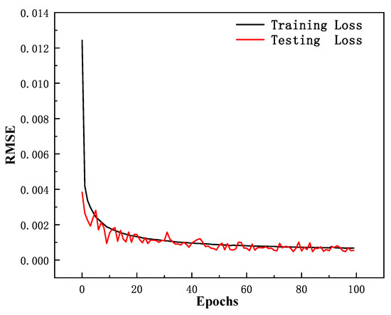
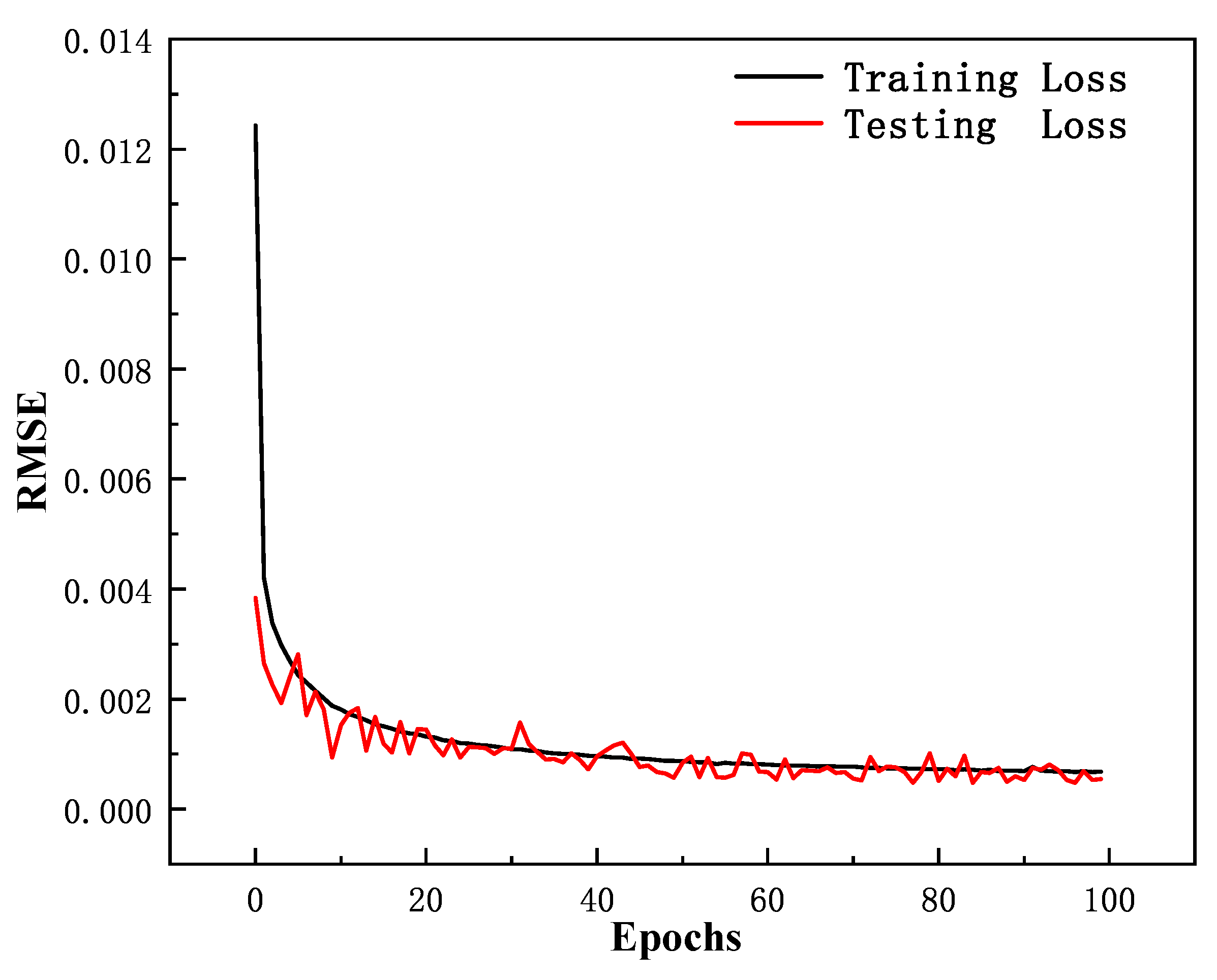
In order to obtain optimal hyperparameters, such as the training epochs and the network layers, we conducted the following experiments. Considering time and computational consumption, we conducted the exploration experiments on hyperparameters within a limited circumstance. We learned the changing trend of training loss and testing loss during training in 100 epochs and try to find the optimal epochs. The details are shown in Figure 4, where we can learn that the losses decrease as the number of epochs increases. We chose to ultimately train 100 epochs. Meanwhile, we explored the impact of the number of LSTM layers in PESO. Table 1 shows the evaluation metrics of PESO under different layers. After comprehensive consideration, we adopted a five-layer LSTM in both encoder and decoder.

Figure 4. The details of training loss and testing loss during the the training process. The X-axis represents the number of training epochs, and the Y-axis represents the RMSE loss value.

Table 1. Explorations on the numbers of LSTM layers under the metrics of RMSE, MAE, ADE, and FDE. Note that 1 layer represents that the number of LSTM layers of encoder and decoder in PESO is 1.

Model	RMSE	MAE	ADE	FDE
1 layer	0.000525	0.000369	0.000581	0.000865
2 layers	0.000614	0.000452	0.000699	0.001008
3 layers	0.000476	0.000325	0.000565	0.000774
4 layers	0.000469	0.000316	0.000542	0.000695
5 layers	0.000466	0.000327	0.000523	0.000681

4.1.3. Baselines

To evaluate the performance of PESO, we make a comparison with several baseline models. RNN baselines models are utilized to predict the 5-track points in a sliding window manner with an input sequence of the previous 10 track points. When the RNN baseline predicts the first track point in the testing period, the process is shown in Equation (14). Note that $Y_{10}$ = ($y_1,y_2,\dots ,y_{10}$), ${\widehat{y}}_{11}$ is the predicted track point, and $\theta$ is the hidden state vector and cell memory.

$${\widehat{y}}_{11}=RNN(Y_{10},\theta )$$

(14)

The twentieth trajectory point is shown in Equation (15) where ${\overline{Y}}_{11}$ = ($y_2,y_3,\dots ,y_{10},{\overline{y}}_{11}$).

$${\overline{y}}_{12}=RNN({\overline{Y}}_{11},\theta )$$

(15)

So we follow the rest of the sequence, and finally, we obtain the output ${\widehat{Y}}_{RNN}$ = (${\overline{y}}_{11},{\overline{y}}_{12},\dots ,{\overline{y}}_{15}$). The seq2seq models in our baselines also predict a sequence of 10 position points but not in a recursive way.

(1)

LSTM. An RNN variant is composed of five layers.

(2)

BiLSTM. An RNN variant is composed of five bidirectional layers.

(3)

GRU. Similar to LSTM.

(4)

BiGRU. Similar to BiGRU.

(5)

LSTM–LSTM. A Seq2Seq-based model with five LSTM layers in the encoder and the decoder. LSTM–LSTM and PESO are both LSTM as the encoder and LSTM as the decoder. The difference is that the input of baseline LSTM–LSTM is longitude and latitude, while PESO’s input includes multiple semantic features and an oriental vector.

(6)

BiLSTM–LSTM. A Seq2Seq-based model with five BiLSTM layers in the encoder and five LSTM layers in the decoder. respectively.

(7)

GRU–GRU. Similar to LSTM–LSTM.

(8)

BiGRU–GRU. Similar to BiLSTM–LSTM.

In addition to RNN-based and Seq2Seq-based methods for trajectory prediction, this paper also considers time-series models. These models include traditional models and deep learning models: Autoregressive Integrated Moving Average model (ARIMA) [38], Kalman Filter [39], Vector Auto-Regression model (VAR) [40], and Spatial and Temporal Normalization (ST-Norm) [41]. Note that the ARIMA, Kalman Filter, and VAR are traditional methods, while ST-Norm is based on neural networks.

(1)

ARIMA. A statistical time-series forecasting model.

(2)

Kalman Filter. A linear optimal estimation model.

(3)

VAR. A statistical model for multivariate time-series prediction.

(4)

ST-Norm. A deep learning model for time-series forecasting.

4.1.4. Evaluation Metrics

We evaluate the performance of the model in our experiments by using the four metrics: Root Mean Square Error (RMSE), Mean Absolute Error (MAE), Final Displacement Error (FDE), and Average Displacement Error (ADE). RMSE is targeted to measure the stability of prediction accuracy and MAE is to evaluate the prediction ability of a model, while ADE and FDE represent the average Euclidean errors between the predicted positions and true ones.

$$\begin{array}{cc}\hfill RMSE& =\sqrt{\frac{1}{n}\sum _{k=1}^n{(y_k-{\widehat{y}}_k)}^2}\hfill \\ \hfill MAE& =\frac{1}{n}\sum _{k=1}^n{\parallel y_k-{\widehat{y}}_k\parallel }_1\hfill \\ \hfill ADE& =\frac{1}{n}\sum _{k=1}^n{\parallel y_k-{\widehat{y}}_k\parallel }_2\hfill \\ \hfill FDE& =\frac{1}{n_T}\sum _{i=1}^{n_T}{\parallel y_i^T-{\widehat{y}}_i^T\parallel }_2\hfill \end{array}$$

(16)

Note that n is the total number of predicted track points, and $n_T$ is the total number of trajectories; $y_k$ and ${\widehat{y}}_k$ denote the real position and the corresponding predicted result, respectively, for the k-th track point; $y_i^T$ and ${\widehat{y}}_i^T$ represent the real position and the predicted position for the last track point of each trajectory; ${\parallel ·\parallel }_1$ is one norm, and ${\parallel ·\parallel }_2$ denotes Euclidean distance. The smaller the value of the metrics, the more accurate the model’s prediction. Note that $y_k$ and $\widehat{y_k}$ are the real and predicted data, respectively, normalized by Min–Max Normalization method for longitude and latitude. The Min–Max Normalization method can be formulated in the following part:

$$x^{\ast }=\frac{x-x_{min}}{x_{max}-x_{min}}$$

(17)

where $x\in X$, $x_{max}$, $x_{min}$ denote the maximum and minimum value in X, respectively, x is the original data, and $x^{\ast }$ is the normalized data.

4.2. Model Performance Comparison

4.2.1. Comparison Results with Baselines

We conducted comparative experiments on baseline models and PESO on RMSE, MAE, and ADE. The LSTM, BiLSTM, GRU, and BiGRU in baselines predict the continuous sequences in sliding window mode, while the other four Seq2Seq models do not. The experimental results under the metric of RMSE, MAE, and ADE are displayed in Table 2, Table 3 and Table 4, respectively. We conducted experiments in 5 scenarios where we predicted from 1 to 5 points using the previous 10 track points. We can see that our model is not the best in the first scenario. We attribute this result to the reason that some baseline models, such as GRU–GRU, have advantages in processing short-track sequences. In the next four scenarios, our model is superior to the baseline models under the three metrics. On the task of long-term prediction, PESO outperforms baselines without doubt.

Table 2. Comparison results with baselines under the metric of RMSE. Here, 10—>5 represents the RMSE value of 5 prediction trajectories through 10 historical trajectories.

Model Name	10—>1	10—>2	10—>3	10—>4	10—>5
LSTM	0.000389	0.000539	0.000728	0.000929	0.001130
BiLSTM	0.000499	0.000643	0.000823	0.001015	0.001210
GRU	0.000395	0.000542	0.000730	0.000929	0.001130
BiGRU	0.000434	0.000570	0.000750	0.000944	0.001141
LSTM-LSTM	0.000380	0.000499	0.000658	0.000844	0.001054
GRU-GRU	0.000326	0.000559	0.000848	0.001163	0.001494
BiGRU-GRU	0.000730	0.000819	0.000938	0.001136	0.001447
BiLSTM-LSTM	0.000571	0.000596	0.000662	0.000747	0.000864
PESO	0.000333	0.000351	0.000378	0.000417	0.000466

Table 3. Comparison results with baselines under the metric of MAE. Here, 10—>5 represents the MAE value of 5 prediction trajectories through 10 historical trajectories.

Model Name	10—>1	10—>2	10—>3	10—>4	10—>5
LSTM	0.000319	0.000415	0.000532	0.000656	0.000780
BiLSTM	0.000380	0.000478	0.000593	0.000714	0.000836
GRU	0.000324	0.000419	0.000532	0.000653	0.000774
BiGRU	0.000341	0.000430	0.000541	0.000660	0.000781
LSTM-LSTM	0.000299	0.000379	0.000483	0.000605	0.000740
GRU-GRU	0.000257	0.000403	0.000581	0.000774	0.000978
BiGRU-GRU	0.000579	0.000640	0.000718	0.000841	0.001021
BiLSTM-LSTM	0.000458	0.000470	0.000510	0.000559	0.000623
PESO	0.000259	0.000267	0.000283	0.000303	0.000327

Table 4. Comparison results with baselines under the metric of ADE. Here, 10—>5 represents the ADE value of 5 prediction trajectories through 10 historical trajectories.

Model Name	10—>1	10—>2	10—>3	10—>4	10—>5
LSTM	0.000493	0.000651	0.000842	0.001043	0.001245
BiLSTM	0.000611	0.000769	0.000956	0.001152	0.001350
GRU	0.000495	0.000650	0.000839	0.001037	0.001238
BiGRU	0.000528	0.000677	0.000860	0.001056	0.001254
LSTM-LSTM	0.000462	0.000587	0.000748	0.000935	0.001139
GRU-GRU	0.000399	0.000649	0.000953	0.001290	0.001649
BiGRU-GRU	0.000914	0.000995	0.001096	0.001256	0.001499
BiLSTM-LSTM	0.000740	0.000753	0.000818	0.000900	0.001007
PESO	0.000412	0.000429	0.000453	0.000484	0.000523

Meanwhile, considering that trajectory prediction task is also a forecasting problem of time series, we compared PESO with several time-series forecasting models, including traditional methods and deep learning models: ARIMA, Kalman Filter, VAR, and ST-Norm, and the comparison results are displayed in Table 5. As we can see from the table, our proposed model is superior to the other time-series forecasting models in four different measurements. We attribute these results to the application of more prior information and the construction of strong spatiotemporal correlation. Different from time-series models utilizing position sequences only, PESO benefits from more prior information, such as speed, travel distance, ship type, and the strong ability to construct spatiotemporal correlations of historical track points.

Table 5. Comparison results with time-series forecasting models under four metrics of RMSE, MAE, ADE, and FDE. The experiments were conducted in the most typical scenario in this paper: predicting the following 5 track points with the previous 10.

Model Name	RMSE	MAE	ADE	FDE
PESO	0.000466	0.000327	0.000523	0.000681
ARIMA	0.001977	0.001675	0.002708	0.003318
Kalman Filter	0.000783	0.000643	0.000989	0.001664
VAR	0.004251	0.002924	0.004701	0.010152
ST-Norm	0.000992	0.000720	0.001133	0.001498

4.2.2. Exploration on Seq2Seq Structure of PESO

At the same time, we explored several experiments on composition structure of the encoder and decoder in PESO to obtain the best performance, including PESO–BiLSTM–LSTM, PESO–GRU–GRU, PESO–BiGRU–GRU, and PESO. As -Table 6 shows, the smallest values of four metrics, RMSE, MAE, ADE, and FDE, are obtained from the structure of PESO, which consists of a Seq2Seq structure of LSTM–LSTM.

Table 6. Exploration results on different Seq2Seq structure.

Model Name	Enc	Dec	RMSE	MAE	ADE	FDE
PESO	LSTM	LSTM	0.000466	0.000327	0.000523	0.000681
PESO-GRU-GRU	GRU	GRU	0.000552	0.000399	0.000646	0.000817
PESO-BiGRU-GRU	BiGRU	GRU	0.000531	0.000387	0.000617	0.000766
PESO-BiLSTM-LSTM	BiLSTM	LSTM	0.000511	0.000380	0.000562	0.000704

4.2.3. Quantitative Analysis

To further explore the detailed prediction error, we performed experiments from the first to the fifth track point and calculated the metrics of RMSE, MAE, and FDE. The prediction results are displayed in Table 7, Table 8 and Table 9.

Table 7. Quantitative results on each track point under the metric of RMSE.

Model Name	First	Second	Third	Fourth	Fifth
LSTM	0.000389	0.000649	0.001000	0.001359	0.001710
BiLSTM	0.000499	0.000757	0.001092	0.001441	0.001785
GRU	0.000395	0.000651	0.001000	0.001358	0.001708
BiGRU	0.000434	0.000672	0.001011	0.001366	0.001712
LSTM-LSTM	0.000380	0.000592	0.000893	0.001245	0.001639
GRU-GRU	0.000326	0.000719	0.001235	0.001801	0.002396
BiGRU-GRU	0.000730	0.000897	0.001133	0.001574	0.002280
BiLSTM-LSTM	0.000571	0.000618	0.000772	0.000952	0.001210
PESO	0.000333	0.000367	0.000425	0.000511	0.000620

Table 8. Quantitative results on each track point under the metric of MAE.

Model Name	First	Second	Third	Fourth	Fifth
LSTM	0.000319	0.000511	0.000767	0.001026	0.001276
BiLSTM	0.000380	0.000577	0.000823	0.001075	0.001322
GRU	0.000324	0.000513	0.000760	0.001013	0.001261
BiGRU	0.000341	0.000519	0.000763	0.001017	0.001266
LSTM-LSTM	0.000299	0.000458	0.000693	0.000971	0.001279
GRU-GRU	0.000257	0.000549	0.000937	0.001354	0.001795
BiGRU-GRU	0.000579	0.000701	0.000874	0.001211	0.001738
BiLSTM-LSTM	0.000458	0.000482	0.000589	0.000709	0.000877
PESO	0.000259	0.000278	0.000314	0.000362	0.000426

Table 9. Quantitative results on each track point under the metric of FDE.

Model Name	First	Second	Third	Fourth	Fifth
LSTM	0.000493	0.000809	0.001225	0.001646	0.002052
BiLSTM	0.000611	0.000927	0.001330	0.001740	0.002140
GRU	0.000495	0.000805	0.001216	0.001634	0.002040
BiGRU	0.000528	0.000825	0.001228	0.001643	0.002046
LSTM-LSTM	0.000462	0.000711	0.001071	0.001494	0.001955
GRU-GRU	0.000399	0.000899	0.001561	0.002299	0.003087
BiGRU-GRU	0.000914	0.001077	0.001296	0.001737	0.002469
BiLSTM-LSTM	0.000740	0.000766	0.000947	0.001147	0.001436
PESO	0.000412	0.000446	0.000501	0.000578	0.000681

In these three tables, we can see that the baseline models have advantages in predicting the first track point, but PESO outperforms other models in the prediction of the next track points, and the prediction errors of all models obviously increase from the first to fifth points. That is because from the first prediction to the last, the amount of information available for a single prediction is obviously decreasing. RNN-baseline models, such as LSTM, use a sliding window manner to predict, which will gradually increase the error and accumulate inaccuracy for each prediction. Seq2Seq-baseline models, such as BiLSTM–LSTM, are capable of predicting several points at one time, reducing the tendency of the increasing error compared to RNN-baseline models.

Our proposed model,, PESO, is specially designed with Parallel Encoders and a Ship-Oriented Decoder. The Parallel Encoders are targeted to capture more feature information by using different encoders to obtain multiple feature representations, which include the Location Encoder and the Sailing Status Encoder. The Parallel Encoders embed different types of features at the same time, avoiding the noise generation of different types of features and enriching feature representation. The Ship-Oriented Decoder utilizes the Semantic Location Vector (SLV) of each ship to guide the prediction, which better represents the spatial correlation of trajectory points. The above two advantages make the proposed PESO model superior to other models.

4.3. Ablation Study

In order to explore each component of PESO, we performed ablation studies on the proposed method. We conducted five groups of different experiments, which are introduced in the following part:

• $Without$ $SOG, COG, and DIS$. Delete the speed, course, and sailing distance on the input of the Sailing Status Encoder of the Parallel Encoders;
• $Without$ $SOG$. Delete the speed on the input of the Sailing Status Encoder of the Parallel Encoders;
• $Without$ $COG$. Delete the course on the input of the Sailing Status Encoder of the Parallel Encoders;
• $Without$ $DIS$. Delete the sailing distance on the input of the Sailing Status Encoder of the Parallel Encoders;
• $Without$ $SLV$. Delete the Semantic Location Vector on the input of the Ship-Oriented Decoder.

Table 10 shows the ablation results. We evaluated the performance under the metrics of RMSE, MAE, ADE, and FDE. It is obvious that the prediction accuracy will drop sharply without the sailing status information of a ship. The course of the vessel determines the direction of the following sailing status to a great extent, and the prediction accuracy will have a negative effect without the nearest course information. Sailing distance and speed denote the endurance and oil storage of a ship. Without these, the sailing status of a ship is not fully expressed, and the prediction performance of the model will be affected. We can also see from the table that the Semantic Location Vector plays a positive role in guiding the prediction process. The Semantic Location Vector in our model better represents the spatial correlation between a ship’s historical trajectory points and forecast ones. Naturally, without the Semantic Location Vector as the guidance information of the decoder, the model will have poor performance. To sum up, the current feature selection of the model is conducive to improving the prediction effect.

Table 10. Ablation studies under the metrics of RMSE, MAE, ADE, and FDE.

Ablation	RMSE	MAE	ADE	FDE
PESO	0.000466	0.000327	0.000523	0.000681
$w/o$  $COG\&SOG\&DIS$	0.000801	0.000576	0.000921	0.001344
$w/o$  $COG$	0.000554	0.000385	0.000621	0.000841
$w/o$  $SOG$	0.000486	0.000342	0.000540	0.000728
$w/o$  $DIS$	0.000474	0.000343	0.000542	0.000711
$w/o$  $SLV$	0.000492	0.000355	0.000563	0.000719

4.4. Case Study

To better demonstrate the visual effect of model prediction, we performed several case studies in this part. Specifically, based on the quantitative prediction results, we expanded on more qualitative results. We display the experiment results of the predicted trajectory in pictorial form in the following parts, which include visual results comparing the baselines, visual results of exploration on the Seq2Seq structure of PESO and qualitative ablation results.

4.4.1. Visual Result Comparing with Baselines

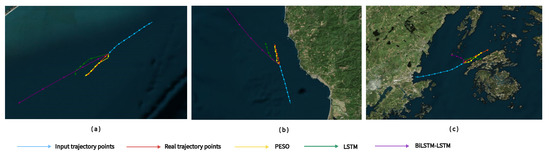
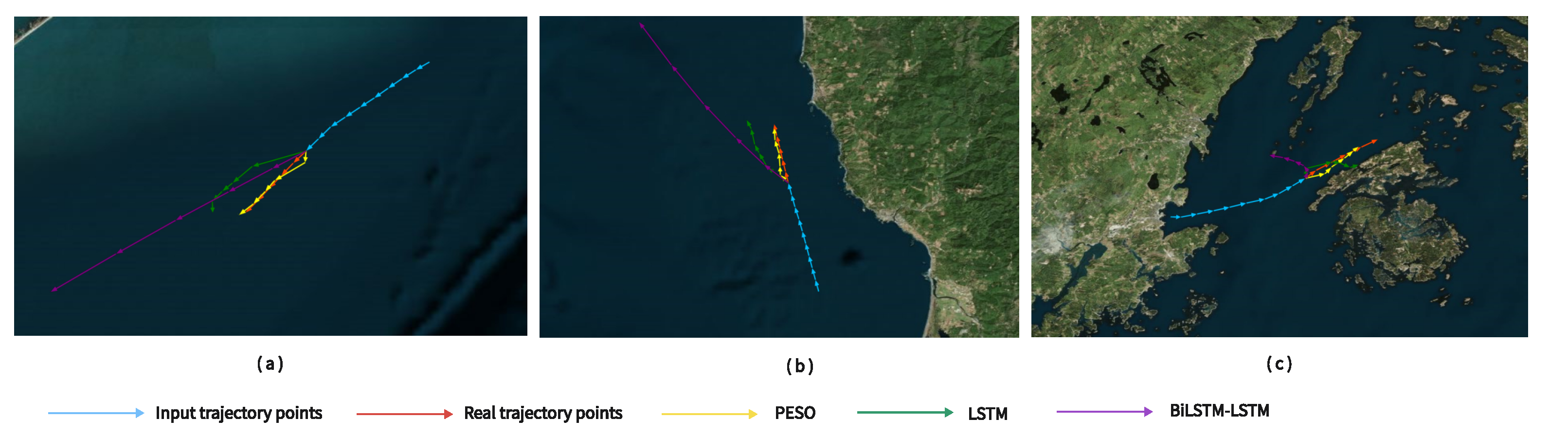
In order to show the prediction results more clearly, we selected the optimum models in RNN baselines and Seq2Seq baselines based on Table 2 and Table 3. LSTM is shown in green lines and BiLSTM-LSTM in purple lines, respectively. We chose three trajectories with 15 random lengths, while 10 track points were for input and 5 for output. The image in Figure 5 shows the visual comparison results on three different trajectories, where the difficulty of the prediction increases gradually. The yellow lines with arrows are the predictions by PESO, while green and purple denote the results of LSTM and BiLST-LSTM, respectively. Blue lines are input trajectory points, and red lines are real ones. As we can see from the images, the trajectories in Figure 5a,b are steady, where PESO is the closest to the real trajectories and performs better than others. Both prediction results by LSTM and BiLSTM in Figure 5a,b are in the wrong directions. In a much more complex scenario in Figure 5c, the other predictions are confusing, while ours is still close to the real one. In reality, incorrect predictions easily cause accidents. Note that the predicted results by PESO are superior to others in the task of vessel trajectory prediction and are able to avoid secure problems.

Figure 5. The visual comparison of different baselines and PESO. The difficulty of prediction increases gradually from (a–c). PESO outperforms other models in all scenarios.

4.4.2. Visual Result of Exploration on Seq2Seq Structure of PESO

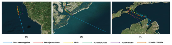
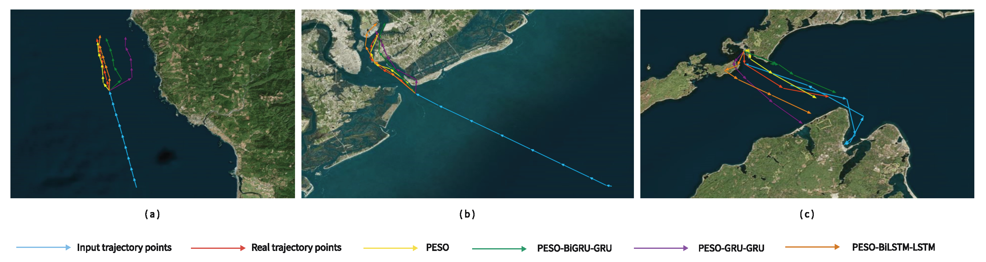
In order to visually show the prediction effects under different Seq2Seq structures, we chose three trajectory sequences randomly. We compared the prediction trajectories with three other models visually, which are PESO–BiLSTM–LSTM, PESO–GRU–GRU, and PESO–BiGRU—GRU. As Figure 6 shows, our model in the LSTM–LSTM structure is more robust in complex scenarios which can avoid accidents. PESO has the ability to predict the track points close to the real ones.

Figure 6. The visual comparison of different structures of PESO. The difficulty of prediction increases gradually from (a–c). As we can see from the figures, PESO (with LSTM–LSTM) can obtain the best prediction results.

4.4.3. Qualitative Ablation Results

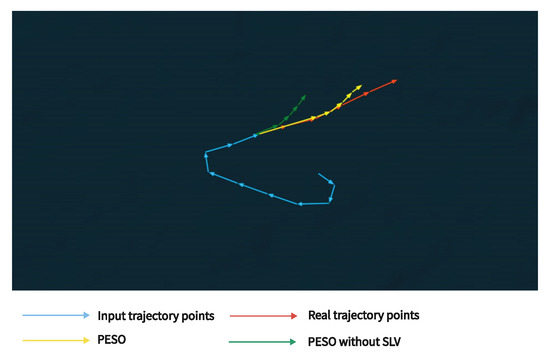
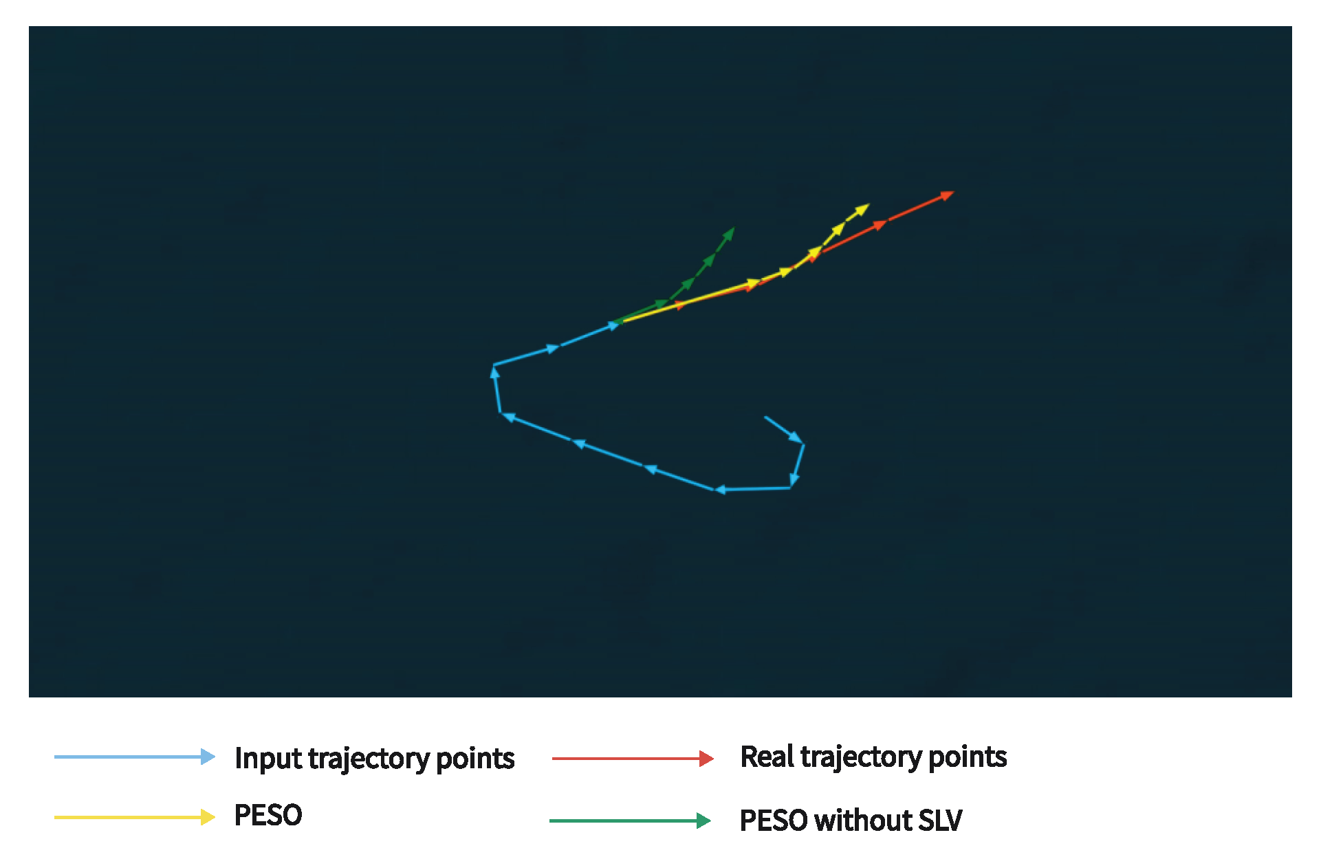
To better present the experimental results visually before and after ablation, we perform a detailed case study in the same trajectory. There are five experiment results on course, speed, sailing distance, and Semantic Location Vector. Moreover, the results are displayed in the five different images. To be precise, we present the visual results of four trajectories on a single image, including input track points, label trajectories, and prediction results before and after ablation. Specifically, in each image, it is clear that the yellow curve and the real trajectory almost overlap.

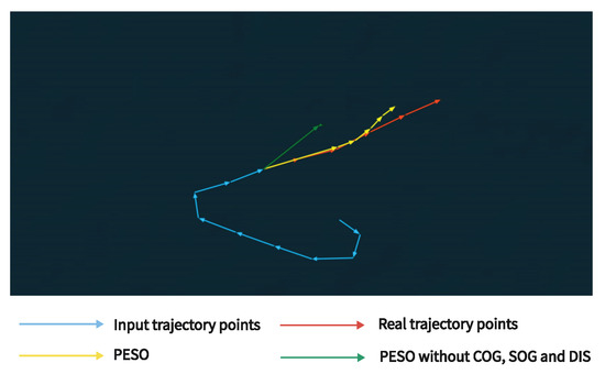
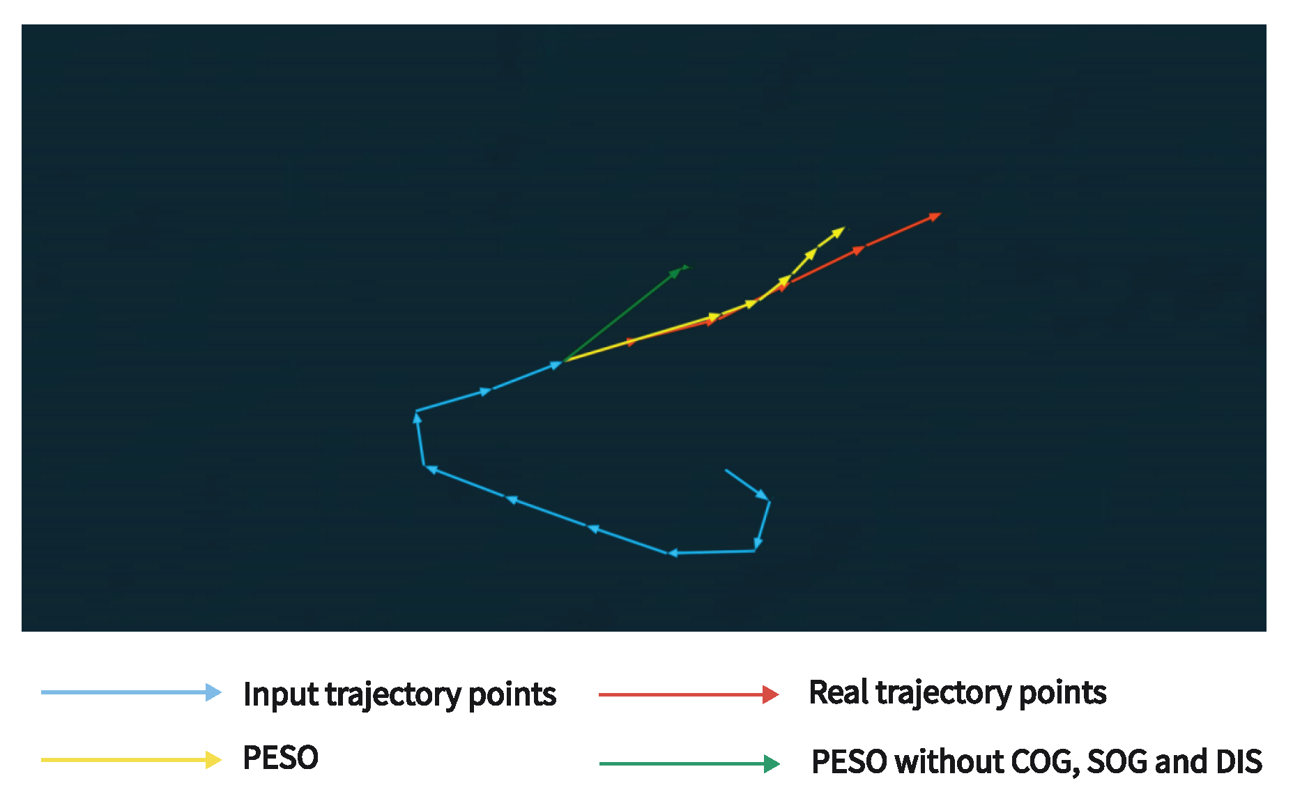
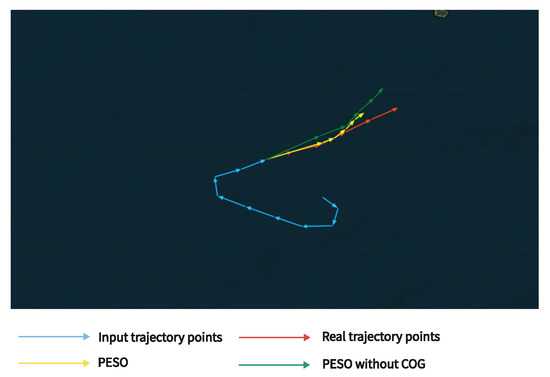
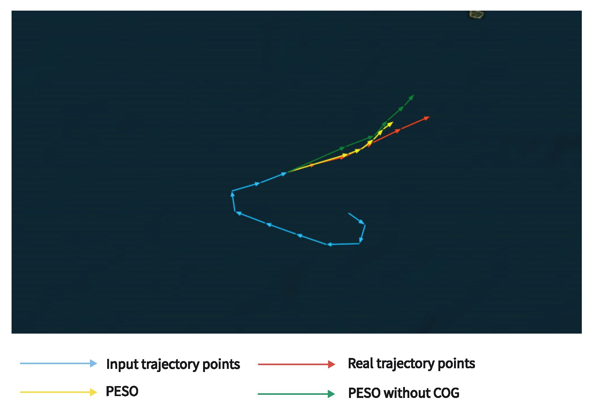
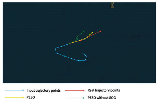
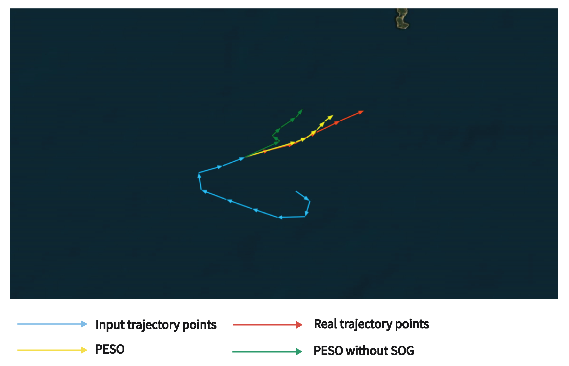
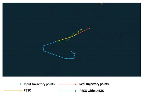
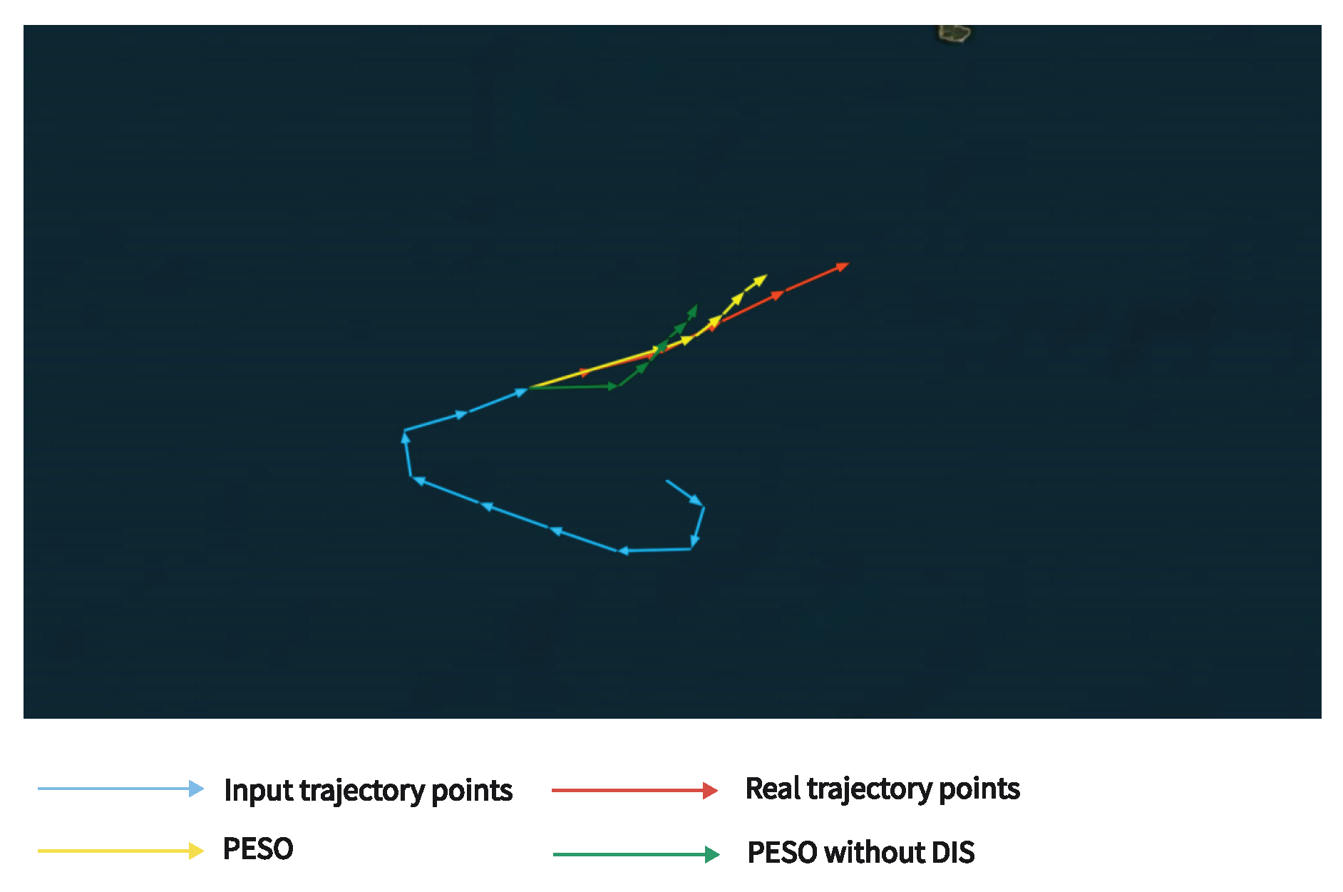
Figure 7 displays the difference with and without the course, speed, and sailing distance in a PESO model. We notice that the prediction results have serious problems in direction and distance without course, speed, and sailing distance of a ship. That is because the model cannot rely only on longitude and latitude to judge the following status. Figure 8 denotes the comparison result with and without course features in a turning corner. The prediction by PESO without a course is in the wrong direction and getting far away from the real one and the yellow one. This is probably because PESO, without course, is unable to identify the sailing direction of the vessel. Figure 9 denotes the comparison result of speed. We suppose that the speed feature helps the model recognize current sailing status. Without speed, the model can easily make a wrong estimation on each timestamp. The PESO model without distance is unable to grasp the sailing distance in every timestamp and makes incorrect predictions in Figure 10. Figure 11 shows the visual comparison results of the Semantic Location Vector. The Semantic Location Vector maintains the spatial correlation between historical and predicted track points. Without the Semantic Location Vector as guidance information for the decoder, the model can easily generate inaccurate predictions due to poor spatial correlation.

Figure 7. The influence of the sailing status information. The yellow and green lines are prediction results of PESO with and without sailing status information, respectively.

Figure 8. The influence of the COG information. The yellow and green lines are prediction results of PESO with and without COG information, respectively.

Figure 9. The influence of the SOG information. The yellow and green lines are prediction results of PESO with and without SOG, respectively.

Figure 10. The influence of the distance information. The yellow and green lines are prediction results of PESO with and without distance information, respectively.

Figure 11. The influence of the SLV. The yellow and green lines are prediction results by PESO with and without SLV, respectively.

From these ablation studies, the accuracy and robustness of the predicted trajectory by PESO are beyond doubt. Moreover, the conducted experiments illustrate that PESO is always capable of predicting satisfying track points.

5. Conclusions

In this paper, we propose a novel trajectory prediction PESO model. PESO consists of Parallel Encoders, a Ship-Oriented Decoder, and a Semantic Location Vector (SLV). The Parallel Encoders are designed to capture more information in feature representation. The Ship-Oriented Decoder is targeted to utilize the SLV to guide the prediction, which better represents the spatial correlation of historical track points. We conducted comparative experiments on several baseline models; the results show that the proposed PESO model outperforms others, both quantitatively and qualitatively. However, it still has some limitations. The data processing of PESO in real-time prediction increases the time consumption. In addition, PESO needs further verification when dealing with more complex scenarios.

6. Future Works

In this study, we focus on enhancing the structure of Seq2Seq networks. In our future works, we will try to adopt other outstanding structures, such as Transformer. Meanwhile, there are many other factors which influence the movement of a vessel. In addition to the factors mentioned in this paper, there are the parameters of the kinematic model of the vessel, the fairway line and its safe width in a given section of movement, the coastline model, etc. In future work, we will add more influencing factors to the modeling process and attempt to conduct further research in a more complex situation.

References

- Capobianco, S.; Forti, N.; Millefiori, L.M.; Braca, P.; Willett, P. Uncertainty-Aware Recurrent Encoder-Decoder Networks for Vessel Trajectory Prediction. In Proceedings of the 2021 IEEE 24th International Conference on Information Fusion (FUSION), Sun City, South Africa, 1–4 November 2021. [Google Scholar]
- Lee, H.T.; Lee, J.S.; Yang, H.; Cho, I.S. An AIS Data-Driven Approach to Analyze the Pattern of Ship Trajectories in Ports Using the DBSCAN Algorithm. Appl. Sci. 2021, 11, 799. [Google Scholar] [CrossRef] [Scilit]
- Mikolov, T.; Chen, K.; Corrado, G.; Dean, J. Efficient Estimation of Word Representations in Vector Space. arXiv 2013, arXiv:1301.3781. [Google Scholar]
- Cho, K.; van Merrienboer, B.; Gülçehre, Ç.; Bahdanau, D.; Bougares, F.; Schwenk, H.; Bengio, Y. Learning Phrase Representations using RNN Encoder-Decoder for Statistical Machine Translation. arXiv 2014, arXiv:1406.1078. [Google Scholar]
- Wilms, H.; Cupelli, M.; Monti, A. Combining auto-regression with exogenous variables in sequence-to-sequence recurrent neural networks for short-term load forecasting. In Proceedings of the 2018 IEEE 16th International Conference on Industrial Informatics (INDIN), Porto, Portugal, 18–20 July 2018. [Google Scholar]
- Razghandi, M.; Zhou, H.; Erol-Kantarci, M.; Turgut, D. Short-Term Load Forecasting for Smart Home Appliances with Sequence to Sequence Learning. In Proceedings of the ICC 2021—IEEE International Conference on Communications, Montreal, QC, Canada, 14–23 June 2021. [Google Scholar]
- Ahmad, T.; Zhang, D. A data-driven deep sequence-to-sequence long-short memory method along with a gated recurrent neural network for wind power forecasting. Energy 2022, 239, 122109. [Google Scholar] [CrossRef] [Scilit]
- Wang, K.; Zhong, H.; Yu, N.; Xia, Q. Nonintrusive Load Monitoring based on Sequence-to-sequence Model With Attention Mechanism. Zhongguo Dianji Gongcheng Xuebao/Proc. Chin. Soc. Electr. Eng. 2019, 39, 75–83. [Google Scholar]
- Fang, Z.; Crimier, N.; Scanu, L.; Midelet, A.; Delinchant, B. Multi-zone indoor temperature prediction with LSTM-based sequence to sequence model. Energy Build. 2021, 245, 111053. [Google Scholar] [CrossRef] [Scilit]
- Sehovac, L.; Nesen, C.; Grolinger, K. Forecasting Building Energy Consumption with Deep Learning: A Sequence to Sequence Approach. In Proceedings of the IEEE International Congress on Internet of Things, Milan, Italy, 8–13 July 2019. [Google Scholar]
- Wang, G.; Zhang, F. A Sequence-to-Sequence Model With Attention and Monotonicity Loss for Tool Wear Monitoring and Prediction. IEEE Trans. Instrum. Meas. 2021, 70, 3525611. [Google Scholar] [CrossRef] [Scilit]
- Yin, H.; Zhang, X.; Wang, F.; Zhang, Y.; Jin, J. Rainfall-Runoff Modeling Using LSTM-based Multi-State-Vector Sequence-to-Sequence Model. J. Hydrol. 2021, 598, 126378. [Google Scholar] [CrossRef] [Scilit]
- Mootha, S.; Sridhar, S.; Seetharaman, R.; Gopalan, C. Stock Price Prediction using Bi-Directional LSTM based Sequence to Sequence Modeling and Multitask Learning. In Proceedings of the 2020 11th IEEE Annual Ubiquitous Computing, Electronics & Mobile Communication Conference (UEMCON), New York, NY, USA, 28–31 October 2020. [Google Scholar]
- Bauer, J.; Jannach, D. Improved Customer Lifetime Value Prediction with Sequence-To-Sequence Learning and Feature-Based Models. ACM Trans. Knowl. Discov. Data (TKDD) 2021, 15, 80. [Google Scholar] [CrossRef] [Scilit]
- Li, X.; Tang, J.; Yin, C. Sequence-to-Sequence Learning for Prediction of Soil Temperature and Moisture. IEEE Geosci. Remote Sens. Lett. 2022, 19, 3005605. [Google Scholar] [CrossRef] [Scilit]
- Zaytar, M.A.; Amrani, C.E. Sequence to Sequence Weather Forecasting with Long Short-Term Memory Recurrent Neural Networks. Int. J. Comput. Appl. 2016, 143, 7–11. [Google Scholar]
- Yin, H.; Guo, Z.; Zhang, X.; Chen, J.; Zhang, Y. Runoff predictions in ungauged basins using sequence-to-sequence models. J. Hydrol. 2021, 603, 126975. [Google Scholar] [CrossRef] [Scilit]
- Hochreiter, S.; Schmidhuber, J. Long short-term memory. Neural Comput. 1997, 9, 1735–1780. [Google Scholar] [CrossRef] [Scilit]
- Tang, H.; Yin, Y.; Shen, H. A model for vessel trajectory prediction based on long short-term memory neural network. J. Mar. Eng. Technol. Proc. Inst. Mar. Eng. Sci. Technol. 2022, 21, 136–145. [Google Scholar] [CrossRef] [Scilit]
- Gao, M.; Shi, G.; Li, S. Online Prediction of Ship Behavior with Automatic Identification System Sensor Data Using Bidirectional Long Short-Term Memory Recurrent Neural Network. Sensors 2018, 18, 4211. [Google Scholar] [CrossRef] [Scilit]
- Wang, C.; Fu, Y. Ship Trajectory Prediction Based on Attention in Bidirectional Recurrent Neural Networks. In Proceedings of the 2020 5th International Conference on Information Science, Computer Technology and Transportation (ISCTT), Shenyang, China, 13–15 November 2020. [Google Scholar]
- Mehri, S.; Alesheikh, A.A.; Basiri, A. A Contextual Hybrid Model for Vessel Movement Prediction. IEEE Access 2021, 9, 45600–45613. [Google Scholar] [CrossRef] [Scilit]
- Ding, M.; Su, W.; Liu, Y.; Zhang, J.; Wu, J. A Novel Approach on Vessel Trajectory Prediction Based on Variational LSTM. In Proceedings of the 2020 IEEE International Conference on Artificial Intelligence and Computer Applications (ICAICA), Dalian, China, 27–29 June 2020. [Google Scholar]
- Wang, C.; Ren, H.; Li, H. Vessel trajectory prediction based on AIS data and bidirectional GRU. In Proceedings of the 2020 International Conference on Computer Vision, Image and Deep Learning (CVIDL), Chongqing, China, 10–12 July 2020. [Google Scholar]
- Capobianco, S.; Forti, N.; Millefiori, L.M.; Braca, P.; Willett, P. Recurrent Encoder-Decoder Networks for Vessel Trajectory Prediction with Uncertainty Estimation. IEEE Trans. Aerosp. Electron. Syst. 2022. [Google Scholar] [CrossRef] [Scilit]
- Nguyen, D.D.; Chan, L.V.; Ali, M.I. Vessel Trajectory Prediction using Sequence-to-Sequence Models over Spatial Grid. In Proceedings of the the 12th ACM International Conference, Hamilton, New Zealand, 25–29 June 2018. [Google Scholar]
- Forti, N.; Millefiori, L.M.; Braca, P.; Willett, P.K. Prediction of vessel trajectories from ais data via sequence-to-sequence recurrent neural networks. In Proceedings of the ICASSP 2020—2020 IEEE International Conference on Acoustics, Speech and Signal Processing (ICASSP), Barcelona, Spain, 4–8 May 2020. [Google Scholar]
- Sekhon, J.; Fleming, C. A Spatially and Temporally Attentive Joint Trajectory Prediction Framework for Modeling Vessel Intent. Learn. Dyn. Control 2020, 318–327. [Google Scholar]
- You, L.; Xiao, S.; Peng, Q.; Claramunt, C.; Zhang, J. ST-Seq2Seq: A Spatio-Temporal Feature-Optimized Seq2Seq Model for Short-Term Vessel Trajectory Prediction. IEEE Access 2020, 8, 218565–218574. [Google Scholar] [CrossRef] [Scilit]
- Capobianco, S.; Millefiori, L.M.; Forti, N.; Braca, P.; Willett, P. Deep Learning Methods for Vessel Trajectory Prediction based on Recurrent Neural Networks. IEEE Trans. Aerosp. Electron. Syst. 2021, 57, 4329–4346. [Google Scholar] [CrossRef] [Scilit]
- Zhang, S.; Wang, L.; Zhu, M.; Chen, S.; Zeng, Z. A Bi-directional LSTM Ship Trajectory Prediction Method based on Attention Mechanism. In Proceedings of the 2021 IEEE 5th Advanced Information Technology, Electronic and Automation Control Conference (IAEAC), Chongqing, China, 12–14 March 2021. [Google Scholar]
- Wang, S.; He, Z. A prediction model of vessel trajectory based on generative adversarial network. J. Navig. 2021, 74, 1161–1171. [Google Scholar] [CrossRef] [Scilit]
- Goodfellow, I.J.; Pouget-Abadie, J.; Mirza, M.; Bing, X.; Warde-Farley, D.; Ozair, S.; Courville, A.; Bengio, Y. Generative adversarial nets. In Proceedings of the Neural Information Processing Systems, Montreal, QC, Canada, 8–13 December 2014. [Google Scholar]
- Nguyen, D.; Fablet, R. TrAISformer-A generative transformer for AIS trajectory prediction. arXiv 2021, arXiv:2109.03958. [Google Scholar]
- Dyer, S.A.; Dyer, J.S. Cubic-spline interpolation. 1. IEEE Instrum. Meas. Mag. 2001, 4, 44–46. [Google Scholar] [CrossRef] [Scilit]
- Shekhar, S.; Hui, X. Root-Mean-Square Error. In Encyclopedia of Gis; Springer: Berlin/Heidelberg, Germany, 2008; p. 979. Available online: https://link.springer.com/referencework/10.1007/978-3-319-17885-1 (accessed on 19 February 2023).
- Kingma, D.; Ba, J. Adam: A Method for Stochastic Optimization. In Proceedings of the 3rd International Conference on Learning Representations, San Diego, CA, USA, May 2015; Available online: http://arxiv.org/abs/1412.6980 (accessed on 19 February 2023).
- Box, G.E.P.; Jenkins, G.M. Time series analysis: Forecasting and control. J. Time 2010, 31, 93–135. [Google Scholar]
- Harvey, A.C. Forecasting, Structural Time Series Models and the Kalman Filter; Cambridge University Press: Cambridge, UK, 1990; pp. 100–167. [Google Scholar]
- Tson, J.C.R.; Parker, R. Vector Autoregressions: Forecasting and Reality. Econom. Rev. 1999, 84, 4. [Google Scholar]
- Deng, J.; Chen, X.; Jiang, R.; Song, X.; Tsang, I. ST-Norm: Spatial and Temporal Normalization for Multi-variate Time Series Forecasting. In Proceedings of the KDD ’21: The 27th ACM SIGKDD Conference on Knowledge Discovery and Data Mining, Virtual, 14–18 August 2021. [Google Scholar]
Disclaimer/Publisher’s Note: The statements, opinions and data contained in all publications are solely those of the individual author(s) and contributor(s) and not of MDPI and/or the editor(s). MDPI and/or the editor(s) disclaim responsibility for any injury to people or property resulting from any ideas, methods, instructions or products referred to in the content. |
© 2023 by the authors. Licensee MDPI, Basel, Switzerland. This article is an open access article distributed under the terms and conditions of the Creative Commons Attribution (CC BY) license (https://creativecommons.org/licenses/by/4.0/).