Climate-State-Dependent Mortality Risk in Smallholder Cattle and Buffalo Systems: An Environmental Systems Model of Livestock Loss, Insurance, and Land Carrying Capacity in Thailand

Abstract

Mortality in smallholder cattle and buffalo systems is climate-driven, but the signal is not uniform: heat and cold stress, flooding, and climate-sensitive disease act through different pathways, yet livestock loss models usually compress them into one elevated-mortality state. The paper builds a climate-state-dependent mortality model for the Thai national herd, separating an endemic baseline from a temperature-extreme and a moisture- and disease-driven regime. A 100,000-iteration Monte Carlo model, calibrated to the 2024 herd and a 2017 farmer survey at 2026 prices, generates the annual loss distribution and decomposes it by driver. The study is a calibrated scenario analysis, not an empirical estimation, so every result is conditional on the calibration and bounded by sensitivity analysis. Endemic mortality governs the average year, about 81% of expected loss but none of the extreme tail; the tail belongs entirely to the two climate regimes, with the moisture- and disease-driven regime carrying roughly 69% of losses beyond the 95th percentile and the temperature regime about 31%. This split holds across low-, medium-, and high-severity scenarios and a baseline range from 0.07 to 0.12, so it is structural: the driver of the typical year is not the driver of the catastrophe. Under a reduced-form behavioral layer with an assumed destocking response, generous payouts would raise stocking pressure 10% to 16% above a sustainable carrying capacity benchmark, so an adaptation instrument could degrade the rangeland it protects. The findings argue for regime-specific risk financing, for pairing insurance with heat and animal health adaptation, and for treating the carrying capacity externality as a design parameter.

1. Introduction

Cattle and water buffalo sit in both the agricultural ecosystem and the household balance sheet across much of the developing world. They convert forage into protein and draught power, recycle nutrients through manure, and store value that households draw down when income fails; the Food and Agriculture Organization [1] estimates that some 600 million smallholder households depend on livestock for part of their food and income. Thailand’s 2024 national herd reached 9.89 million beef cattle and 1.81 million buffalo [2], more than double the 2016 totals [3], across close to a million households. When animals die at scale, food, savings, and the breeding stock needed to rebuild are lost at once, so livestock mortality is an environmental systems problem, not only an insurance one.

Environmental pressure on these systems is rising. Warming has already cut agricultural output and raised its variance [4,5], and 2024 was the warmest year in the instrumental record [6]. For livestock, the most direct channel is thermal load: heat stress depresses feed intake, impairs fertility, and at sufficient intensity raises mortality [7]. Extreme heat exposure is projected to rise across domesticated species through this century [8], and cattle sector heatwave exposure climbs under climate scenarios even in temperate zones, with grazing and housed systems exposed differently [9]. The cold tail matters too: cold snaps have killed large numbers of cattle and buffalo in upland Lao PDR, the same Mekong zone as northeastern Thailand [10]. A second channel is moisture and disease, as flooding and shifting vector ranges move pathogens; the regional record shows repeated transboundary outbreaks of foot-and-mouth disease, lumpy skin disease, and hemorrhagic septicemia [11,12,13,14,15,16,17,18] that cluster losses across herds in a way a constant mortality rate cannot represent. Section 2 develops both channels.

Most analyses of livestock mortality risk nonetheless treat elevated mortality as a single-epidemic state on a constant baseline [19,20]. That simplification hides a question with direct policy content: which climate driver dominates the average year, and which dominates the catastrophe? The two need not coincide, and the answer shapes where surveillance, early warning, and adaptation money should go. Chen, Maneejuk, and Yamaka [21], modeling Chinese grain systems, find that agricultural insurance is climate-state-dependent, substitutive under temperature shocks and complementary under precipitation shocks, so the right mix of insurance and physical adaptation varies with the type of climate stress. Splitting the elevated regime by driver brings that logic into livestock loss modeling.

A further question is ecological. Insurance is promoted as a climate adaptation instrument [22,23,24], but it is not ecologically neutral. John et al. [25], in an agent-based model of East African pastoralism, show that drought insurance can suppress the destocking herders would otherwise undertake after a shock, holding stocking density above carrying capacity and degrading rangeland over time. Gehring and Schaudt [26] find a related land-use channel, with insured herders less likely to drive animals onto cropland when forage fails, and Bulte and Lensink [27] argue more generally that insurance can dampen risk-reducing behavior. An instrument meant to protect a livestock ecosystem can thus place new pressure on it.

This paper develops both questions in one transparent, reproducible framework, built as a calibrated scenario analysis rather than an empirical estimation, because the data needed to estimate the climate regime parameters directly do not yet exist at national scale. The framework conditions Thai cattle and buffalo mortality on a climate state index, decomposes the annual loss distribution by climate driver, and traces how mortality insurance design feeds back onto destocking and land carrying capacity. Its contribution is fourfold. First, where standard livestock loss models collapse every elevated peril into a single-epidemic state, this model separates a temperature-extreme regime and a moisture- and disease-driven regime from the endemic baseline, a strict generalization that nests the conventional two-regime model as a limiting case. Second, it introduces a decomposition, new to the livestock loss literature, that identifies which climate driver owns the mean and which owns the tail. Third, it makes the ecological externality of mortality insurance explicit and measurable for free-range smallholder systems, a setting the rangeland–pastoralism evidence has not addressed. Fourth, it documents the model, calibration, and code for replication. The claims are deliberately bounded: the parameters are calibrated and stated openly, the consequential ones varied by sensitivity and scenario analysis, and the paper is a foundation to be revised, not a closed result. A Supplementary Materials document provides the derivations, extended results, robustness analyses, and code.

2. Climate, Disease Ecology, Demand, and the Ecology of Insurance

The relevant literature spans four areas usually treated separately: the climatic and biological drivers of mortality, the demand-side behavior that determines whether insurance reaches farmers, the fiscal and structural performance of programs, and the ecological consequences of insurance itself. Conditioning mortality on climate state and letting insurance feed back onto land draws on all four, and the review is organized by driver because separating drivers is the analytical move the rest of the paper makes. The demand and fiscal material is kept brief, confined to what the later sections use.

2.1. Temperature Extremes and Ruminant Mortality

The physiology of heat stress in ruminants is well characterized: elevated thermal load shifts animals from production toward thermoregulation, disrupts redox balance, and damages cellular and metabolic function, so growth, reproduction, and immune competence decline before death [7]. Because these early losses are sublethal, heat stress is increasingly tracked through production metrics and animal-level sensing rather than mortality alone, since milk yield, growth, and intake respond continuously to thermal load [28], and heat sensitivity carries a genetic component that selection shifts only slowly [29]. A model that prices mortality therefore captures a lower bound on the climate burden, since the intake, fertility, and growth losses that precede death are real costs it omits. Thornton et al. [8] project rising extreme heat exposure across domesticated species through this century, and See [9] shows cattle sector heatwave exposure rising under climate scenarios, with grazing and housed systems exposed differently, a distinction that bears on the land-use channel developed later. For tropical beef cattle, Schuck-Paim et al. [30] quantify heat stress welfare across South American locations using the Comprehensive Climate Index, identify a thermal threshold above which mortality rises even in healthy animals, and show shade provision to be cost-effective, so heat stress can be physically reduced as well as insured. The cold tail is real too, since Khounsy et al. [10] document significant cold stress mortality of large ruminants in northern and central Lao PDR, the same upland Mekong zone as northeastern Thailand, where large ruminant health is constrained by feed and housing [31]. What the literature does not provide is a single annual mortality rate for tropical cattle and buffalo that could enter a national loss model directly, since it depends jointly on temperature, humidity, breed, body condition, management, and diurnal range, so the temperature regime severity is calibrated here and flagged for estimation rather than asserted.

2.2. Moisture, Flooding, and Climate-Sensitive Disease Emergence

The second elevated regime is driven by moisture and disease. Foot-and-mouth disease is endemic to mainland Southeast Asia, and its reporting tracks animal movement along the Mekong corridor [11,12]; regional and global reviews document recurrent serotype turnover and cross-border transmission [13,14], and exotic strains have repeatedly emerged on Greater Mekong smallholder farms where biosecurity is limited and trade links are dense [15]. Lumpy skin disease, a vector-borne pathogen sensitive to temperature and moisture, spread across Southeast and South Asia from 2019 and caused large cattle losses in newly affected areas [16,17], and hemorrhagic septicemia, tied to wet-season conditions, remains a leading cause of buffalo death in the region [18]. Two features drive the modeling. First, these events are correlated across herds and cluster in time, generating a heavy upper tail rather than a thicker spread around the mean. Second, several pathogens are climate-sensitive in range or seasonality, so the regime’s frequency is not fixed but plausibly rising, the direction the heat stress literature also gives for temperature. Regional movement and trade compound the signal, since animals cross borders along market chains and a local outbreak can become regional within a season [12,15]. The regime is thus more severe and more spatially contagious than the temperature one, which a future spatial extension should capture. One caution carries into the calibration: the outbreak studies report case fatality rates within affected herds, whereas the model needs an annual herd-level rate blended across affected and unaffected animals, so the elevated regime severity is set deliberately below reported case fatalities.

2.3. Insurance as a Climate Adaptation Instrument

Livestock and agricultural insurance is widely placed in the climate adaptation toolkit, and the case rests on demand and design. Uptake tends to rise after climatic shocks as experience updates risk perception [24], and index designs are promoted to manage climate risk while limiting moral hazard and verification cost [23,32,33,34]. Composite indices combining temperature, precipitation, and vegetation signals are proposed to separate drivers and lower the basis risk that has undermined single-index products [22], while the political economy of climate insurance complicates matters, since the instrument redistributes risk among farmers, insurers, and the state [35,36]. The development record is mixed: coverage has expanded rapidly, but uptake in low- and middle-income settings stays below self-sustaining levels and the evidence on its development promise is uneven [37,38]. Foundational treatments of livestock revenue and income insurance establish the contract structures these products build on [39,40,41], and regional syntheses cover the design choices specific to Asian agriculture [42].

2.4. Demand, Fiscal Performance, and Structural Effects

Two further bodies of evidence bound what insurance-based adaptation can achieve. On demand, willingness to pay rises with herd size, education, and prior loss and often exceeds the subsidized premium [43], while trust, subsidy level, indemnity alignment, claim settlement speed, and credit access shape participation [44,45]; gender matters, with women responding strongly to bundled products [46,47], and inflated expectations and weak claim settlement are recurring failure modes [48,49]. Reviews of African and Asian programs find that subsidy expansion alone does not move uptake without parallel investment in data, distribution, and trust [50,51], that supply-side willingness to offer cover responds to incentives as much as demand does [52], and that even sophisticated producers under-cover, so producer education carries a return alongside subsidy [53]. On fiscal grounds, compressing loadings below sustainable levels trades short-run affordability for long-run insolvency [54], subsidy expansion creates fiscal dilemmas and can be captured by sophisticated participants [55,56], and fiscal incentives can reduce rural inequality, more so in poorer regions [57], while sustainability depends less on subsidy generosity than on administrative efficiency and linkage with extension, credit, and cooperative channels [58,59]. Two structural cautions complete the picture: insurance may slow agricultural transformation by dampening risk-reducing investment [27], and livestock often serve as the buffer asset, so formal cover can substitute for the informal risk management that sustains it [60,61]. The model takes two implications forward: the insured share is endogenous and policy-sensitive, and the generosity that strains the public balance sheet also drives the grazing-pressure channel, so fiscal and ecological costs move together.

2.5. Ecological Externalities of Livestock Insurance

The ecological channel is the least studied and the most central here. The core mechanism is destocking suppression: after a shock, uninsured herders sell or move animals to match stocking to forage, but insured herders, expecting indemnity, retain them and keep grazing pressure high, degrading carrying capacity over time [25]. Gehring and Schaudt [26] add field evidence of a land-use externality, insured pastoralists being less likely to encroach on cropland during forage failure, and Bulte and Lensink [27] place these findings in a frame in which insurance crowds out risk-reducing behavior. The coping portfolio literature sharpens the point: where livestock are the informal buffer, formal cover can displace the destocking that keeps the system within ecological limits [60,61]. These externalities are documented mainly for extensive rangelands; whether they carry over to free-range smallholder systems, and how they interact with a climate state mortality structure, has not been modeled.

2.6. Synthesis and Open Questions

Four gaps follow. Climate driver heterogeneity is rarely built into livestock loss models, which collapse distinct perils into one elevated state and so cannot say which driver owns the tail. Demand heterogeneity is studied apart from aggregate risk, so the endogeneity of the insured share seldom feeds into exposure modeling. Fiscal analysis quantifies subsidy cost but rarely connects it to the ecological consequences of the same generosity. And the ecological externality, identified for rangelands, has not been quantified for free-range smallholder systems or linked to a climate-conditioned mortality structure. The framework below addresses the first and fourth gaps directly and is built so the second and third can be added later.

Table 1. Environmental drivers, mortality regimes, and supporting evidence.

Environmental Driver	Mechanism for Livestock Loss	Mortality Regime	Representative Evidence
Heat and cold extremes	Thermoregulatory and metabolic failure; rising heatwave exposure; cold snap kills	Temperature (T)	Belhadj Slimen et al. [7]; Thornton et al. [8]; Schuck-Paim et al. [30]; Hasan et al. [28]; Gayari et al. [29]; See [9]; Khounsy et al. [10]
Flooding and vector-borne disease	Clustered, correlated outbreak mortality (FMD, LSD, HS)	Moisture and disease (M)	Madin [11]; Smith et al. [12]; Aslam and Alkheraije [13]; Brito et al. [14]; Bin-Tarif et al. [15]; Wilhelm and Ward [16]; Sudhakar et al. [17]; World Organisation for Animal Health [18]
Endemic background	Routine, near-independent mortality	Baseline (B)	Boyd, Pai and Porth [19]; Pai, Boyd and Porth [20]
Insurance behavior	Destocking suppression; raised grazing pressure	Carrying capacity layer	John et al. [25]; Gehring and Schaudt [26]; Bulte and Lensink [27]; Hänke and Barkmann [60]

maps drivers to regimes and to the corpus evidence grounding each.

3. The Climate-State-Dependent Mortality Model

The model generalizes a regime-switching mortality engine into a climate-conditioned form and adds a reduced-form behavioral layer linking insurance design to destocking and land carrying capacity, presented so it can be reimplemented from the equations alone.

3.1. Individual Mortality and Indemnity

Index insured animals by $i=1,\dots ,N$. The annual mortality indicator $D_i\in \left\{\mathrm{0,1}\right\}$ equals one if animal $i$ dies during the policy year. With per-head insured value $V$ and coverage ratio $\alpha \in \left(\mathrm{0,1}\right]$, the indemnity on death is $I_i=\alpha V{D}_i$, and expected indemnity per animal under mortality rate $p$ is $\mathbb{E}\left[I_i\right]=\alpha Vp$. The accuracy of any premium or exposure figure built on this identity depends entirely on $p$, and small errors in $p$ scale into large aggregate imbalances when applied across a national herd [62]. Treating $p$ as a single constant is therefore the weak point, because mortality in these systems is neither constant nor stationary [19,20]. The revenue and income insurance literature reaches the same conclusion from the contract side, since pricing that ignores the structure of the loss distribution misprices the product [39,40].

3.2. Climate-Conditioned Regimes

Let a climate state index $R_t$ govern the policy year $t$:

$$R_t\in \{B,\hspace{0.25em}T,\hspace{0.25em}M\},$$

where $B$ is the endemic baseline, $T$ the temperature-extreme regime (heat or cold stress), and $M$ the moisture- and disease-driven regime. These three states are the model’s primitives rather than quantities recovered from data, and each simulated year is assigned to exactly one of them by a single draw from a categorical distribution with probabilities

$$\mathrm{P}\mathrm{r}\left(R_t=B\right)=1-{\theta }_T-{\theta }_M, \mathrm{P}\mathrm{r}\left(R_t=T\right)={\theta }_T, \mathrm{P}\mathrm{r}\left(R_t=M\right)={\theta }_M.$$

Conditional on the regime, the herd mortality rate is drawn from a truncated normal,

$$p_t\mid R_t=r\hspace{0.25em}\sim \hspace{0.25em}\mathcal{N}\left({\mu }_r,\hspace{0.25em}{\sigma }_r^2\right), \mathrm{truncated}\mathrm{to}\left[0,1\right],$$

with ${\mu }_B=p_b$ and ${\mu }_T,{\mu }_M>p_b$. The truncated normal is a parsimonious choice that keeps the mean and dispersion of each regime interpretable while preventing impossible mortality rates. Because mortality proportions are bounded and can be skewed, the choice of severity distribution is itself a modeling assumption, and Section 5 reports that replacing the truncated normal with a beta distribution matched on the same regime means and dispersions moves the 95th and 99th percentiles by less than half a percent, so the tail metrics are not an artifact of the distributional form; heavier-tailed alternatives are discussed in Section 8. A single systemic draw $p_t$ scales the whole insured herd, which encodes the correlation that makes climate and disease shocks dangerous, since a bad year is bad for the pool as a whole and not for independent animals. Aggregate annual loss is

$$L_t=\alpha \hspace{0.17em}\left(N^c{V}^c+N^b{V}^b\right)\hspace{0.17em}{p}_t,$$

for cattle ($c$) and buffalo ($b$) insured populations $N^c,N^b$. The model nests the conventional two-regime structure because setting ${\theta }_M=0$ and ${\mu }_T=p_e$ recovers a single elevated epidemic regime, so the climate state model is continuous with, rather than a departure from, standard livestock loss modeling. One structural assumption should be flagged at the outset rather than left to the limitations. The three regimes are mutually exclusive within a year, so a season that combines heat stress and a disease outbreak is not represented, and because those drivers are positively correlated under warming, the assumption understates the joint upper tail rather than inflating it, which makes the reported tail a conservative reading of the compound risk. The regime severities and frequencies are calibrated, not estimated, and bounded by the sensitivity and scenario analysis in Section 5.

3.3. Regime Decomposition of Loss

The new quantitative objects are the shares of expected and of tail loss attributable to each regime. Writing $q_{0.95}$ for the 95th percentile of $L_t$,

$$s_r^{\mathrm{mean}}={\displaystyle \frac{\mathrm{P}\mathrm{r}\left(R_t=r\right)\hspace{0.17em}\mathbb{E}\left[L_t\mid R_t=r\right]}{\mathbb{E}\left[L_t\right]}}, s_r^{\mathrm{tail}}={\displaystyle \frac{\mathbb{E}\left[L_t\hspace{0.17em}1\left(R_t=r,\hspace{0.25em}{L}_t>q_{0.95}\right)\right]}{\mathbb{E}\left[L_t\hspace{0.17em}1\left(L_t>q_{0.95}\right)\right]}}.$$

Here $s_r^{\mathrm{mean}}$ is the fraction of total expected loss attributable to regime $r$, and $s_r^{\mathrm{tail}}$ is the fraction of aggregate loss beyond the 95th percentile attributable to regime $r$, where $1\left(\cdot \right)$ is the indicator function that selects the iterations in the named regime and above the threshold. The mean share answers which driver dominates the typical year, and the tail share answers which dominates the catastrophe. Separating the two is the analytical payoff of conditioning mortality on climate state, because it converts a single loss distribution into a statement about attribution, and it is the object most directly useful to other researchers.

3.4. Insurance, Destocking, and Carrying Capacity Pressure

The behavioral layer follows the John et al. [25] mechanism in reduced form. After a shock of severity $p_t$, the surviving herd is $N\left(1-p_t\right)$. Herders choose a destocking fraction $d_t$, the additional animals sold to relieve grazing pressure and smooth consumption. Insurance generosity, the product of coverage $\alpha$ and subsidy $s$, lowers the incentive to destock, because the indemnity substitutes for the cash that a distress sale would raise:

$$d_t\left(\alpha ,s\right)=d_0\hspace{0.17em}\left(1-\varphi \hspace{0.17em}\alpha \hspace{0.17em}s\right),$$

with $d_0$ the baseline destocking fraction absent insurance and $\varphi \in \left[0,1\right]$ the suppression strength. Define the land-carrying capacity pressure index as standing stock relative to the sustainable benchmark $K=N\left(1-p_b\right)\left(1-d_0\right)$, the stocking implied by endemic mortality with normal adaptive destocking:

$$\Pi \left(\alpha ,s\right)={\displaystyle \frac{\mathbb{E}\left[\hspace{0.17em}1-p_t\hspace{0.17em}\right]\hspace{0.17em}\left(1-d_t\left(\alpha ,s\right)\right)}{\left(1-p_b\right)\left(1-d_0\right)}}.$$

The index is a normalized, dimensionless indicator, the ratio of stocking under a given insurance design to stocking under the uninsured adaptive benchmark, and not an operational stocking rate measurement in animals per hectare, so values above one mean stocking pressure above the sustainable benchmark rather than a forecast of forage depletion. Generosity raises $\alpha s$, lowers $d_t$, and pushes $\Pi$ above one, which is the John et al. degradation channel applied to a free-range smallholder setting. The specification is kept minimal so that its drivers are transparent, since the result depends on the sign of $\varphi$, not its exact value, and the comparative statics in $\alpha$ and $s$ hold for any $\varphi >0$. Two caveats are explicit. The mechanism is calibrated and stylized rather than estimated for Thailand, and the original evidence is extensive Kenyan rangeland, whereas Thai cattle and buffalo are roughly 90% free-range smallholder systems [63], so $\Pi$ is an indicator of direction and order of magnitude, not an ecological forecast. The direction is supported independently by the land-use and behavioral evidence [26,27].

3.5. Simulation Procedure and Convergence

The model is solved by Monte Carlo. Each of the 100,000 iterations draws a regime from the categorical distribution over the three states, draws a herd mortality rate from the corresponding truncated normal, and computes the aggregate loss. Because iterations are independent, the empirical distribution approximates the annual loss distribution, and expected loss, standard deviation, percentiles, and the conditional tail expectation are read off as sample statistics, with regime shares obtained by tagging each iteration with its generating regime. A fixed seed makes every figure and table reproducible. Sampling error is small: the standard error of the mean is about 0.15 million USD against a mean of 121 million, and tail quantiles stay stable across seeds, since the 10% combined frequency of the elevated regimes places about 10,000 iterations in the two climate regimes and several hundred beyond the 99th percentile. Seed stability and convergence are documented in the Supplementary Materials (Sections S6.1 and S6.2).

4. Data and Calibration

4.1. Herd, Values, and Exposure

Calibration uses an established single-country dataset for Thai cattle and buffalo, drawn entirely from published national statistics and a published farmer survey, so it is reproducible from public sources. Herd populations are the 2024 Department of Livestock Development figures, 9.89 million beef cattle and 1.81 million buffalo [2]. Per-head values come from the 2017 Bank for Agriculture and Agricultural Cooperatives survey of 665 cattle and buffalo farmers across four provinces [63], inflated to 2026 by 11.5% cumulative Thai consumer price inflation [64] at 31.10 baht per US dollar, giving 1091.37 USD per head of cattle and 1073.53 USD per head of buffalo. Household participation is set at 50% and the within-household coverage factor at 0.2125, the survey anchor, so the insured population is about 1.05 million cattle and 0.19 million buffalo, with an insured value at risk near 1083 million USD at the 80% coverage used for the loss distribution scenario. Participation is held fixed, though Section 2.4 shows it is endogenous, and the model accepts a participation schedule if the analysis is extended.

The two species are carried in a single blended herd rather than modeled separately, and the reason is worth stating because cattle and buffalo differ in heat tolerance, in susceptibility to hemorrhagic septicemia, in market value, and in management. The blended treatment is a deliberate simplification licensed by the structure of the model and the data. Aggregate loss is linear in the insured value at risk, so with the per-head values and populations of both species entered separately in $L_t$, a common mortality regime prices the herd correctly to the extent that the herd-average bad-year mortality is similar across the two, which the regional veterinary record does not contradict at the coarse annual, national scale used here. The available primary survey [63] does not report species-specific mortality by climate driver, so a species split would have to introduce parameters with no anchor, trading a transparent simplification for a hidden assumption. Species-specific severities and a buffalo-weighted disease regime are a natural extension once the mortality data described in Section 8 exist, and the code is structured to accept them.

The survey predates the analysis, which warrants comment. The 2017 Bank for Agriculture and Agricultural Cooperatives study is the only nationally stratified primary survey of smallholder cattle and buffalo husbandry, asset values, and insurance preferences in Thailand, so it is the best source for the per-head values and the coverage factor. Its structural parameters are slow-moving, since herd composition, free-range prevalence, and the sector’s institutional structure have not shifted materially since 2017, so those findings carry forward even where prices do not; only monetary values are updated, by 11.5% inflation over 2017 to 2026 [64], with herd totals from the 2024 release [2]. Two developments since the survey, lumpy skin disease and a run of climate extremes, both cut toward higher elevated-regime risk, so treating the 2017 structure as unchanged is conservative for the tail. As an external check, the elicited willingness to pay, 2.4% to 4.9% of indemnity, sits inside the contemporary range reported for Canada [20], Nepal [43], and Nigeria [33].

4.2. Regime and Behavioral Parameters

The climate state parameters appear in

Table 2. Climate state mortality calibration.

Parameter	Symbol	Value	Provenance
Baseline mortality	$p_b$	0.100	Calibrated (project)
Baseline dispersion	${\sigma }_B$	0.020	Calibrated (project)
Temperature regime mean	${\mu }_T$	0.200	Calibrated, anchored in heat and cold stress evidence
Temperature regime dispersion	${\sigma }_T$	0.040	Calibrated
Temperature regime probability	${\theta }_T$	0.050	Calibrated, anchored in heatwave exposure projections
Moisture/disease regime mean	${\mu }_M$	0.240	Calibrated, anchored in outbreak evidence
Moisture/disease regime dispersion	${\sigma }_M$	0.050	Calibrated
Moisture/disease regime probability	${\theta }_M$	0.050	Calibrated, anchored in outbreak frequency
Baseline destocking fraction	$d_0$	0.150	Stylized
Insurance suppression strength	$\varphi$	1.000	Stylized
Monte Carlo iterations	$S$	100,000	Fixed seed for reproducibility

with a provenance column separating measured anchors from calibrated assumptions. Baseline mortality and its dispersion are the project calibration, consistent with routine smallholder mortality in the regional veterinary record [31]. The two elevated regimes split the conventional single-epidemic regime: their probabilities sum to 0.10 and their mean mortality averages 0.22, so the model reproduces the aggregate elevated regime while resolving it into two drivers. The moisture- and disease-driven regime is given the higher mean and dispersion because clustered outbreaks of foot-and-mouth, lumpy skin disease, and hemorrhagic septicemia produce the heaviest correlated losses [16,18], while the temperature regime is given a lower sustained mean, consistent with heat and cold stress mortality operating alongside large production and fertility losses rather than only death [7,30], and its frequency is the parameter most likely to rise under warming [8,9]. Combining several perils into one state is intentional, since what they share is clustered, correlated bad-year mortality with a heavy tail; a peril-by-peril or seasonal extension should recover the differences in seasonality, transmission, and control (Section 8).

4.3. The Status of the Calibration and How the Results Depend on It

The parameters in Table 2 are calibrated rather than estimated, and the distinction governs how the results are read: every number below is a scenario output conditional on this calibration, not an empirical estimate of Thai livestock loss. No source known to the author reports an annual climate-attributable mortality rate for tropical cattle and buffalo at national scale; the heat stress literature measures exposure, welfare, production, and fertility rather than a herd mortality rate [7,8,28,30], and the disease literature documents outbreaks, ranges, and case fatality rather than a standing annual severity [11,16,17]. Calibration is therefore the only option until those data exist, and stating the values openly and bounding the consequential ones with sensitivity analysis is what keeps it honest.

The anchor that carries the most weight is the aggregate elevated regime, not any single cell: the two climate regimes are built so their probabilities sum to 0.10 and their severities average 0.22, the conventional single-epidemic regime of standard livestock loss modeling, reflecting the veterinary record for foot-and-mouth disease, lumpy skin disease, and hemorrhagic septicemia in affected populations during bad years [16,17,18], set deliberately below the within-outbreak case fatality rates those studies report. Because the model collapses to this single regime when the split is removed, the mean, variance, and unconditional percentiles match the standard model; the split resolves only their internal composition, which is what licenses the claim that the decomposition, not the loss level, is the contribution.

The division of that regime into a temperature state and a disease state is the genuinely new assumption, made conservatively. The temperature mean is set below the disease mean, 0.20 against 0.24, at equal annual probabilities of 0.05. Keeping the means close is deliberate: it ensures the finding that the disease regime carries the larger tail share is not built in by an assumed severity gap but emerges from its higher dispersion and the geometry of the loss distribution. What the literature does not supply is the precise magnitude of either severity, which the model treats as a quantity to be varied, as the low-, medium-, and high-severity scenarios in Section 5 do.

The baseline mortality of 0.10 is the parameter most open to dispute, and it is flagged as such. A 10% blended annual rate is high for intensive systems but defensible for the low-input, free-range smallholder herds that dominate the Thai sector, where about 90% of farmers run free-range systems [63], veterinary access is uneven, and endemic disease is a constant background [19,31]. It remains a calibration, and a reviewer preferring 0.07 or 0.08 would have a reasonable case, but the consequence, set out in Section 5, is smaller than it appears, because the baseline governs the center of the distribution, while the tail belongs to the elevated regimes. The within-regime dispersions, 0.02 for the baseline and 0.04 and 0.05 for the elevated regimes, capture year-to-year variation around each mean, with the elevated regimes given larger dispersions because outbreak and heatwave severity vary more than routine mortality.

The behavioral parameters, the baseline destocking fraction of 0.15 and the suppression strength of 1.0, are the weakest entries and are labeled stylized. They have no literature anchor, since the destocking response of free-range smallholders to mortality insurance has not been measured, and the motivating evidence is extensive pastoralism rather than the Thai setting [25]. Their role is to show the direction and plausible order of magnitude of the externality, not to estimate it: the sign and the comparative statics in coverage and subsidy hold for any positive suppression strength, while the specific 10% to 16% figure is illustrative. The path from calibration to estimation is set out in Section 8, and until those data exist the calibration is offered as a transparent, reproducible base case, designed to be revised rather than believed.

5. Environmental Loss Distribution by Climate Regime

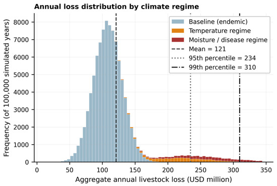
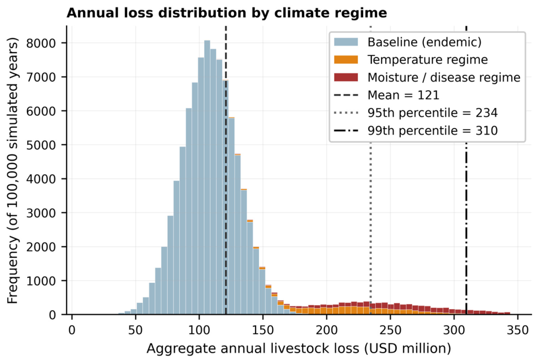
The Monte Carlo generates the aggregate annual loss distribution and its regime decomposition, each a scenario output conditional on the Table 2 calibration. Mean annual loss is 121.0 million USD, with a standard deviation of 47.1 million. The distribution is right-skewed: the 95th percentile is 234.5 million, the 99th 309.7 million, the 99.5th 330.3 million, and the conditional expectation beyond the 99th percentile 337.2 million;

Table 3. Loss distribution and regime decomposition.

Quantity	Baseline (B)	Temperature (T)	Moisture/Disease (M)	All
Share of years	0.90	0.05	0.05	1.00
Share of expected loss	0.81	0.09	0.11	1.00
Share of tail loss (>95th pct)	0.00	0.31	0.69	1.00
Conditional mean loss (USD m)	108	216	261	121
Aggregate mean (USD m)				121.0
95th percentile (USD m)				234.5
99th percentile (USD m)				309.7
99% CTE (USD m)				337.2

collects these aggregate quantiles alongside the regime decomposition below. The simulated mean matches the analytical expected loss, the insured value at risk of 1083 million USD times mean mortality of 0.112, confirming the simulation is unbiased and that splitting the elevated regime leaves aggregate exposure unchanged while revealing its internal structure. A variance decomposition reinforces this: about 70% of year-to-year variance comes from which regime occurs rather than variation within a regime (Supplementary Section S3.6). Extended quantiles and the exceedance curve appear in Supplementary Tables S2 and S3 and Figure S1.

Figure 1 colors the distribution by the regime that generated each simulated year. The bulk near the mean is almost entirely baseline mortality; the long right tail is built from the two climate regimes, which barely overlap the central mass.

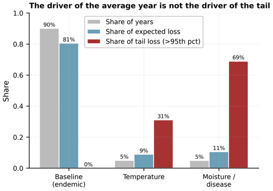
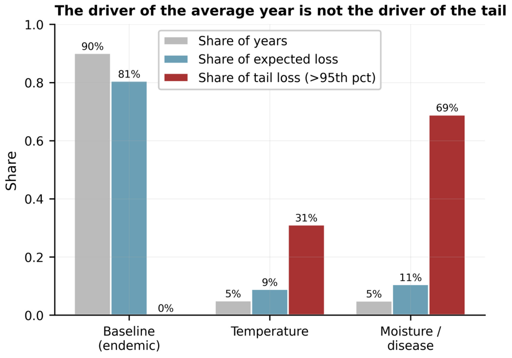
The decomposition shows this directly (Figure 2), and Table 3 sets out the full decomposition with the conditional loss in each regime. The baseline regime occurs in about 90% of years and accounts for 81% of expected loss but none beyond the 95th percentile, because routine mortality never reaches catastrophic magnitude under the calibrated dispersion. The temperature regime occurs in 5% of years, contributes 9% of expected loss, and carries 31% of tail loss, at a conditional mean of 216 million USD. The moisture- and disease-driven regime occurs in 5% of years, contributes 11% of expected loss, and carries 69% of tail loss, at a conditional mean of 261 million. The driver of the average year, endemic mortality, contributes nothing to the catastrophe, while the two climate regimes that barely register in the mean own the entire tail, the disease regime roughly twice the temperature regime, whose frequency the heat stress evidence indicates will rise [8,9]. A risk manager who budgets from the mean prepares for the wrong event.

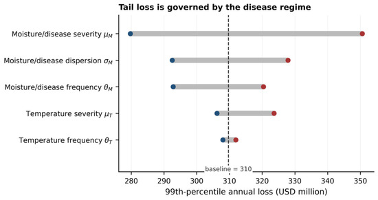
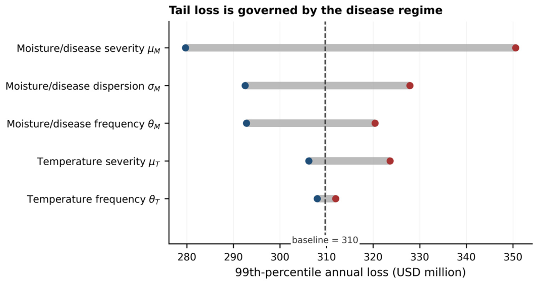
The sensitivity of the 99th-percentile loss to the elevated-regime parameters appears in Figure 3. Varying the moisture and disease regime mean from 0.20 to 0.28 moves the 99th percentile from 280 to 351 million USD, by far the widest swing, with dispersion and frequency next. The temperature regime parameters move the tail less because that regime sits lower in severity, though its rising frequency under warming is the relevant forward risk. The tail is governed by the disease regime, which tells risk managers and researchers where recalibration and surveillance investment buy the most precision: a better estimate of disease regime severity is worth more, for tail accuracy, than a better estimate of any other single parameter.

The attribution result is a structural property of the calibration, not an artifact of the chosen levels or of sampling noise, and

Table 4. Robustness of the loss distribution to the calibration and to the severity distribution. Loss figures in USD million; tail shares are the shares of loss beyond the 95th percentile carried by the baseline, temperature, and moisture/disease regimes.

Variant	Mean	95th pct	99th pct	99% CTE	Tail Share B/T/M
Low severity (temperature 0.16, disease 0.20)	116.7	191.2	266.4	293.9	0.00/0.31/0.69
Medium severity (base: 0.20, 0.24)	121.0	234.5	309.7	337.2	0.00/0.31/0.69
High severity (temperature 0.24, disease 0.28)	125.3	277.8	353.0	380.5	0.00/0.31/0.69
Baseline mortality 0.07	91.7	234.5	309.7	337.2	0.00/0.31/0.69
Baseline mortality 0.12	140.5	234.5	309.7	337.2	0.00/0.31/0.69
Beta severity (matched mean and dispersion)	121.2	233.8	310.1	341.7	0.00/0.31/0.69

makes this concrete by rerunning the model under alternative calibrations and an alternative severity distribution. Varying the two elevated-regime means together across low-, medium-, and high-severity scenarios scales the dollar tail, the 99th percentile moving from 266 to 353 million USD, but leaves the tail-share decomposition at 0, 31, and 69% throughout, so the scenarios move the magnitude of the catastrophe without touching its composition. Varying the baseline mortality from 0.07 to 0.12 rescales the mean loss from 92 to 141 million but leaves every tail quantile and regime share unchanged, because the baseline mass sits entirely below the 95th percentile. This answers the concern that the baseline’s zero tail share is mechanical: it is, in the precise sense that a regime bounded below the threshold cannot enter the tail, and that boundedness survives a baseline as high as 0.12. Replacing the truncated normal with a matched beta moves the 95th and 99th percentiles by less than half a percent and the tail expectation by about 1%, so the tail is not an artifact of the distributional form. Across all three exercises, the calibration controls the level of the tail, not its composition, which is why the decomposition is the contribution and why disease regime severity is the parameter worth estimating first.

External plausibility deserves comment, since the model is calibrated and cannot be validated in the strict sense. No Thai national series of insured payouts or climate-attributable herd mortality exists to validate the loss distribution against, and that absence is itself the central data gap the paper points to. What can be done is a consistency check against the corpus outbreak record. The elevated-regime severities used here, a herd-average bad-year mortality of 0.20 to 0.24, sit below the within-outbreak case fatality rates reported for foot-and-mouth disease, lumpy skin disease, and hemorrhagic septicemia [16,17,18], as they should, since a herd-average blends affected and unaffected animals whereas a case fatality rate conditions on infection. The conditional loss in a disease year, 261 million USD, is about a fifth of the insured value at risk, the order of magnitude the record associates with a severe regional outbreak season along the Mekong corridor [11,12]. This is a consistency check, not a validation: it shows the calibrated severities are not implausible against the evidence, and names the payout and mortality series that would turn it into a test.

6. Insurance Design, Destocking, and Land Carrying Capacity

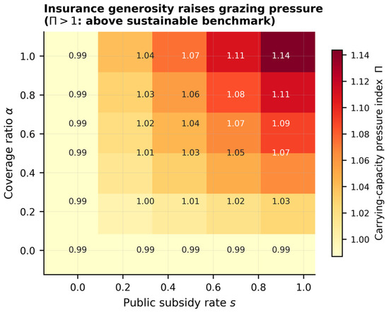
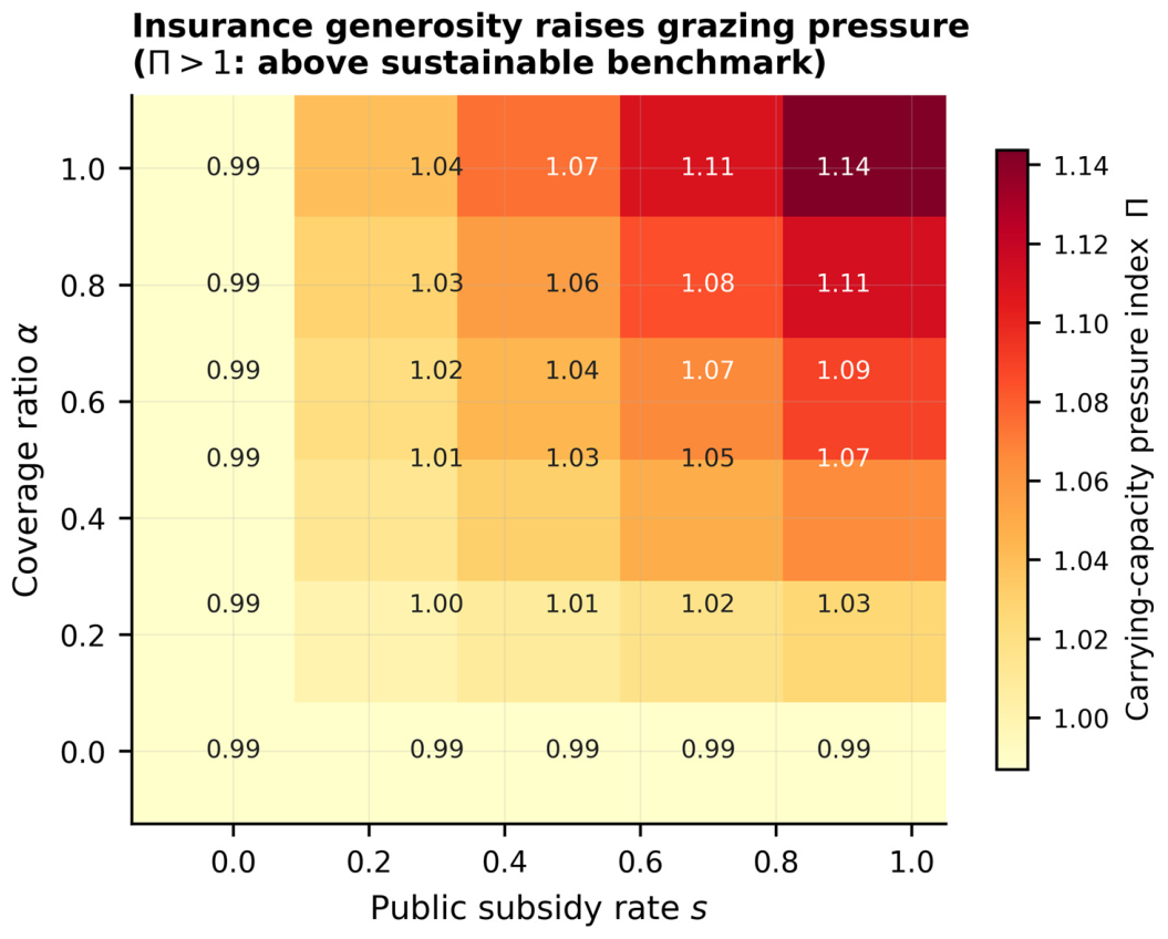
The behavioral layer converts insurance generosity into a land-carrying capacity outcome. Figure 4 shows the pressure index $\Pi$ over the grid of coverage $\alpha$ and subsidy $s$. With no coverage, $\Pi$ sits at 0.99, just below the sustainable benchmark, because mortality itself thins the herd and farmers destock normally. As generosity rises, $\Pi$ climbs. At a coverage ratio of 0.8 and a subsidy of 0.7, settings within the range of real programs, $\Pi$ reaches 1.08, about 10% above the uninsured benchmark, and at full coverage and a 0.9 subsidy it reaches 1.14, about 16% above. The pattern is monotone in both levers and steepest where coverage and subsidy are simultaneously high, exactly the configuration that subsidy-driven expansion produces, and exactly the configuration that the fiscal literature warns is most exposed to capture and cost overrun [54,55]. The full pressure-index grid is tabulated in Supplementary Table S9. The index should be read as the relative indicator defined in Section 3.4, a ratio of stocking under a given design to stocking under the uninsured adaptive benchmark, and not as an operational carrying capacity in animals per hectare, which would require the forage, rainfall, and land-access data the model does not use.

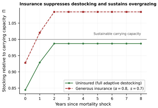
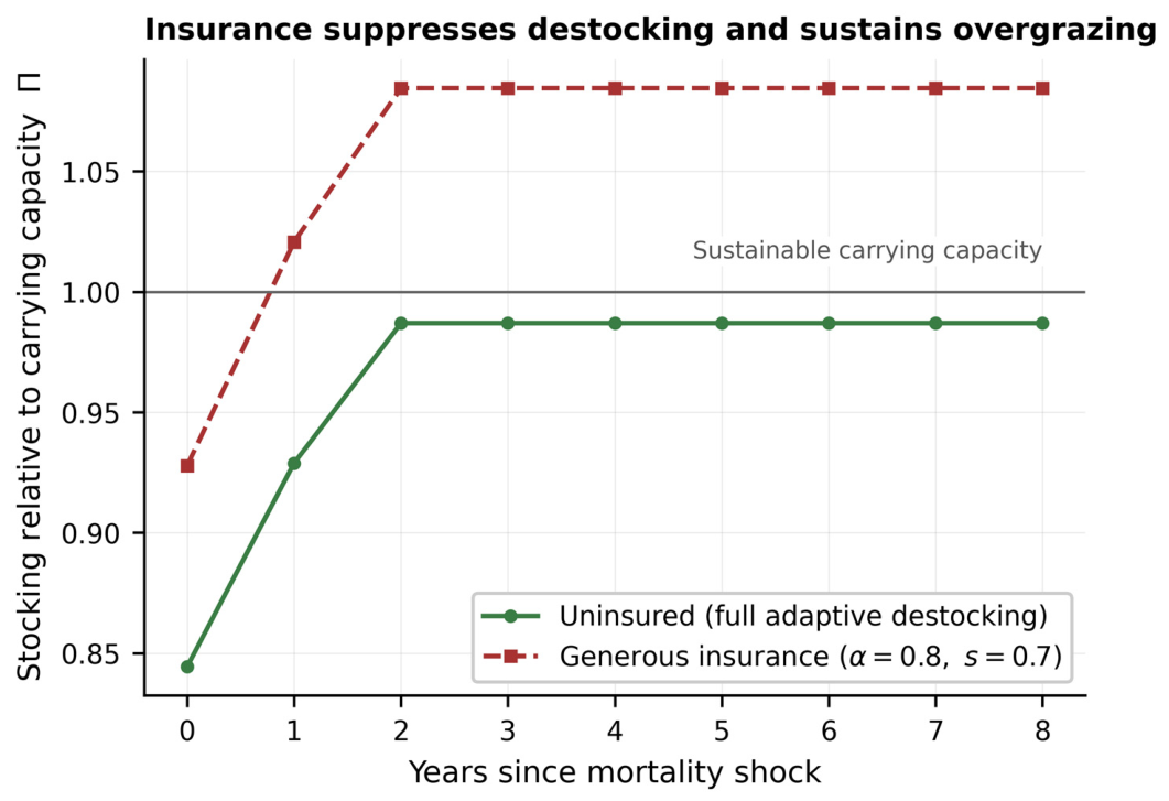
Figure 5 traces the dynamic version. After a severe mortality shock, an uninsured herd recovers toward the sustainable benchmark and settles just below it, because adaptive destocking keeps stocking matched to forage, while a herd under generous insurance recovers past the benchmark and stabilizes above it, sustaining the overgrazing the destocking would otherwise prevent. The gap between the paths is the ecological cost of suppressing adaptive behavior, the channel John et al. [25] identify and Bulte and Lensink [27] generalize, and it compounds, since each year spent above carrying capacity erodes the forage base that sets the benchmark, so a static index understates a dynamic cost.

The result should be read with its caveats. The magnitudes are stylized, the suppression strength and baseline destocking fraction are assumed, and the source mechanism is rangeland pastoralism rather than Thai free-range smallholding [63]. What the model establishes is qualitative and robust to them: across the entire plausible range of the suppression parameter, more generous payouts raise grazing pressure, so the ecological footprint of livestock insurance is a design choice, not a fixed property of the instrument. The land-use evidence supports the sign independently [26], and the coping portfolio evidence suggests the displaced behavior is the informal management that holds these systems within ecological limits [60]. Insurance relieves the liquidity motive behind a distress sale, its intended benefit, but also removes the ecological discipline the sale imposed, since animals that would have been sold remain on a forage base the shock has already reduced. The response is therefore to price or condition the externality, and how large the effect is depends on how much of the destocking was ecologically adaptive rather than financial, the quantity the Section 8 extension is designed to recover.

7. Policy and Decision Support Implications

Three implications follow for the design of climate-resilient livestock systems, each framed to be acted on with the information a national program already has.

First, risk financing should be regime-specific. Since endemic mortality owns the average year and the climate regimes own the tail, the predictable and catastrophic layers call for different instruments: retained reserves and routine premiums for the baseline, pre-arranged contingent financing for the temperature and disease tails. A flat product priced on average loss misprices both, a known failure of expected loss pricing under correlated shocks [20,65] long flagged for revenue and income products [39,41]. The decomposition also shows where surveillance buys the most tail precision, the disease regime, while the temperature regime, whose frequency is rising, is the one to monitor for structural change [8,9].

Second, insurance should be paired with physical adaptation, not offered as a substitute. The climate state dependence Chen, Maneejuk and Yamaka [21] document for crop systems applies here: insurance and adaptation are complements under some shocks and substitutes under others, so the right policy is a portfolio. For the temperature regime, shade provision is cost-effective in tropical beef systems [30], and grazing and housed systems face different heat exposure [9]; for the disease regime, vaccination, movement control, and surveillance along the Mekong corridor address the loss at its source [11,12]. Composite climatic indices can underpin credible triggers that separate drivers and lower basis risk [22]. None of this reaches farmers without attention to trust, claim settlement, and information channels, the binding constraints the uptake literature identifies [43,44,50].

Third, the carrying capacity externality belongs in the contract. If generous payouts suppress destocking and degrade rangeland, payout design should internalize that cost, for instance through destocking or pasture management conditionality on indemnity, which John et al. [25] motivate directly and which fits the bundled products farmers already accept [47]. This reframes a subsidy question usually argued on fiscal and equity grounds [54,55,56,57] as an environmental management question too, since the same generosity that raises fiscal exposure raises grazing pressure. The case rests on ecosystem resilience and land carrying capacity under warming, which the evidence here supports directly, and needs no greenhouse gas accounting frame.

These steps can be sequenced. The cheapest is diagnostic, applying regime decomposition to a country’s own mortality and climate records to see whether its tail is disease-led, as in the Thai calibration, or temperature-led, which determines whether early money goes to surveillance or heat adaptation. The next is to structure financing in layers that match the decomposition, and the last, most often skipped, is to write the carrying capacity and adaptation conditions into the contract from the outset, since retrofitting them onto an established subsidized product is politically harder than building them in. None requires data a national livestock authority does not already collect.

8. A Research Agenda for Climate State Livestock Loss Modeling

The agenda below is organized by the constraint each item relaxes; the documented model, calibration, and code let each be attempted without rebuilding the framework.

Direct estimation of climate regime mortality. Replacing the calibrated regime severities with estimates is the most valuable extension and is becoming feasible: animal-level sensing paired with climate indices can estimate heat and cold stress mortality functions [28], the Comprehensive Climate Index supplies a thermal metric with a documented mortality threshold [30], and veterinary surveillance series support disease regime estimation [11,16]. A panel of provincial mortality against climate and outbreak covariates would turn every parameter in Table 2 into an estimate, and a national payout series would supply the external benchmark the model now lacks.

Species-specific and multi-peril resolution. Once species- and peril-specific data exist, the same engine can carry separate cattle and buffalo severities and resolve the disease regime into its seasonal parts, testing how much the blended treatment costs in tail accuracy.

Mortality and the wider productivity burden. The model prices only mortality; pairing it with a production loss function estimated from animal-level sensing and welfare evidence [28,30] would let a contract be designed against the full climate cost, including the sublethal losses in intake, fertility, growth, and milk that precede death.

Compound and time-varying regimes. Treating regimes as mutually exclusive understates the joint tail; compound regimes or climate-weighted mixtures would capture the correlation warming strengthens, since it raises both heat exposure [8] and vector-borne disease range [16], and regime probabilities indexed to a warming trend would let the tail grow with the climate.

Spatial structure and basis risk. Resolving the national model to the province level, with spatial correlation for climate and disease, would show how much diversification a national pool provides and let index product basis risk be quantified against the simulated loss field [22].

Estimating the behavioral layer. The destocking response is the most stylized element; its suppression strength is estimable from household panels on herd sales around shocks or a coverage-varying field experiment [46,47,48], and a Thai forage-and-stocking calibration would turn the pressure index from an indicator into a measurement.

Welfare, distribution, and the public balance sheet. The loss distribution feeds questions this paper leaves open: the welfare value of cover, its incidence across herd sizes and genders, and its contingent cost to the state; the fiscal and demand literature supplies the components [43,54,55,57], and the regime decomposition the risk structure they need.

Cross-country transfer and open tooling. The structure is portable, since smallholder cattle and buffalo systems across South Asia, Sub-Saharan Africa, and Latin America share the mortality and fiscal constraints that motivate it [37,38]; documented at the level of its equations and parameters, it can be forked, recalibrated, and audited.

9. Conclusions

Livestock mortality in smallholder cattle and buffalo systems is a climate and land-use problem, and modeling it as such changes what the numbers say. Separating the elevated-mortality state into a temperature-extreme regime and a moisture- and disease-driven regime leaves aggregate exposure unchanged but reveals that endemic mortality, the driver of the average year, contributes nothing to the catastrophe, while two climate regimes that barely register in the mean own the entire tail, split roughly two to one between disease and temperature. The split holds across low-, medium-, and high-severity scenarios and a baseline mortality range from 0.07 to 0.12, so it is structural. Under the reduced-form behavioral layer, generous payouts would suppress adaptive destocking and lift grazing pressure 10% to 16% above a sustainable benchmark, so an adaptation instrument can degrade the system it protects.

The limits are stated plainly, and they define the research program as much as the results do. The climate regime severities and frequencies are calibrated rather than estimated, so the paper is a scenario analysis whose dollar figures are conditional on the calibration. The model prices mortality as a lower bound because the losses that precede death are not counted, and it treats regimes as mutually exclusive within a year, so a combined heat-and-disease season is not represented and the tail on that count is understated. Mortality enters as a single systemic shock scaling the whole insured herd, and cattle and buffalo are blended, so the behavioral layer indicates direction rather than magnitude. Section 8 sets out how each limit can be relaxed. Insurance is, in the end, one element of a climate adaptation portfolio for livestock ecosystems, and its ecological footprint is something to design, not to discover after the fact.

References

- Food and Agriculture Organization of the United Nations. World Food and Agriculture: Statistical Yearbook 2022; FAO: Rome, Italy, 2022; Available online: https://openknowledge.fao.org/server/api/core/bitstreams/0c372c04-8b29-4093-bba6-8674b1d237c7/content (accessed on 15 May 2026).
- Department of Livestock Development. Thailand Country Presentation; WOAH Regional Representation for Asia and the Pacific: Tokyo, Japan, 2024; Available online: https://rr-asia.woah.org/app/uploads/2024/04/3.4-Thailand_Country-presentation.pdf (accessed on 13 June 2026).
- Department of Livestock Development. Livestock Population Statistics of Thailand; Ministry of Agriculture and Cooperatives: Bangkok, Thailand, 2016.
- Lobell, D.B.; Schlenker, W.; Costa-Roberts, J. Climate trends and global crop production since 1980. Science 2011, 333, 616–620. [Google Scholar] [CrossRef] [Scilit] [PubMed]
- Ortiz-Bobea, A.; Ault, T.R.; Carrillo, C.M.; Chambers, R.G.; Lobell, D.B. Anthropogenic climate change has slowed global agricultural productivity growth. Nat. Clim. Change 2021, 11, 306–312. [Google Scholar] [CrossRef] [Scilit]
- World Meteorological Organization. State of the Global Climate 2024; WMO: Geneva, Switzerland, 2025. [Google Scholar]
- Belhadj Slimen, I.; Najar, T.; Ghram, A.; Abdrrabba, M. Heat stress effects on livestock: Molecular, cellular and metabolic aspects, a review. J. Anim. Physiol. Anim. Nutr. 2016, 100, 401–412. [Google Scholar] [CrossRef] [Scilit] [PubMed]
- Thornton, P.; Nelson, G.; Mayberry, D.; Herrero, M. Increases in extreme heat stress in domesticated livestock species during the twenty-first century. Glob. Change Biol. 2021, 27, 5762–5772. [Google Scholar] [CrossRef] [Scilit] [PubMed]
- See, L. Future heatwave exposure of the European cattle sector. npj Sustain. Agric. 2026, 4, 6. [Google Scholar] [CrossRef] [Scilit]
- Khounsy, S.; Nampanya, S.; Inthavong, P.; Yang, M.; Khamboungheung, B.; Avery, M.; Bush, R.D.; Rast, L.; Windsor, P.A. Significant mortality of large ruminants due to hypothermia in northern and central Lao PDR. Trop. Anim. Health Prod. 2012, 44, 835–842. [Google Scholar] [CrossRef] [Scilit] [PubMed]
- Madin, B. An evaluation of foot-and-mouth disease outbreak reporting in mainland South-East Asia from 2000 to 2010. Prev. Vet. Med. 2011, 102, 230–241. [Google Scholar] [CrossRef] [Scilit] [PubMed]
- Smith, P.; Luthi, N.B.; Huachun, L.; Oo, K.N.; Phonvisay, A.; Premashthira, S.; Abila, R.; Kukreja, K.; Bounma, P.; Win, H.H.; et al. Movement Pathways and Market Chains of Large Ruminants in the Greater Mekong Sub-Region; FAO Animal Production and Health Working Paper; FAO: Rome, Italy, 2015. [Google Scholar]
- Aslam, M.; Alkheraije, K.A. The prevalence of foot-and-mouth disease in Asia. Front. Vet. Sci. 2023, 10, 1201578. [Google Scholar] [CrossRef] [Scilit] [PubMed]
- Brito, B.P.; Rodriguez, L.L.; Hammond, J.M.; Pinto, J.; Perez, A.M. Review of the global distribution of foot-and-mouth disease virus from 2007 to 2014. Transbound. Emerg. Dis. 2017, 64, 316–332. [Google Scholar] [CrossRef] [Scilit] [PubMed]
- Miller, C.A.; Young, J.R.; Nampanya, S.; Khounsy, S.; Singanallur, N.B.; Vosloo, W.; Abila, R.; Hamilton, S.A.; Bush, R.D.; Windsor, P.A. Risk factors for emergence of exotic foot-and-mouth disease O/ME-SA/Ind-2001d on smallholder farms in the Greater Mekong Subregion. Prev. Vet. Med. 2018, 159, 115–122. [Google Scholar] [CrossRef] [Scilit] [PubMed]
- Wilhelm, L.; Ward, M.P. The spread of lumpy skin disease virus across Southeast Asia: Insights from surveillance. Transbound. Emerg. Dis. 2023, 2023, 3972359. [Google Scholar] [CrossRef] [Scilit] [PubMed]
- Sudhakar, S.B.; Mishra, N.; Kalaiyarasu, S.; Jhade, S.K.; Hemadri, D.; Sood, R.; Bal, G.C.; Nayak, M.K.; Pradhan, S.K.; Singh, V.P. Lumpy skin disease (LSD) outbreaks in cattle in Odisha state, India. Transbound. Emerg. Dis. 2022, 69, e2723–e2731. [Google Scholar] [CrossRef] [Scilit] [PubMed]
- World Organisation for Animal Health. Haemorrhagic Septicaemia; Technical Disease Card; WOAH: Paris, France, 2021; Available online: https://www.woah.org/app/uploads/2021/09/haemorrhagic-septicemia.pdf (accessed on 13 June 2026).
- Boyd, M.; Pai, J.; Porth, L. Livestock mortality insurance: Development and challenges. Agric. Financ. Rev. 2013, 73, 233–244. [Google Scholar] [CrossRef] [Scilit]
- Pai, J.; Boyd, M.; Porth, L. Insurance premium calculation using credibility analysis: An example from livestock mortality insurance. J. Risk Insur. 2015, 82, 341–357. [Google Scholar] [CrossRef] [Scilit]
- Chen, Y.; Maneejuk, P.; Yamaka, W. Grain production resilience under climate shocks in China depends on agricultural insurance and farmland infrastructure. Front. Sustain. Food Syst. 2026, 10, 1845760. [Google Scholar] [CrossRef] [Scilit]
- Kalantaripor, M.; Najafi Alamdarlo, H.; Mosavi, S.H.; Vakilpoor, M.H. Designing and evaluating a composite climatic index for risk management in livestock insurance. Environ. Sustain. Indic. 2025, 28, 101025. [Google Scholar] [CrossRef] [Scilit]
- Madaki, M.Y.; Kaechele, H.; Bavorova, M. Agricultural insurance as a climate risk adaptation strategy in developing countries: A case of Nigeria. Clim. Policy 2023, 23, 747–762. [Google Scholar] [CrossRef] [Scilit]
- Senapati, A.K. Insuring against climatic shocks: Evidence on farm households’ willingness to pay for rainfall insurance product in rural India. Int. J. Disaster Risk Reduct. 2020, 42, 101351. [Google Scholar] [CrossRef] [Scilit]
- John, F.; Toth, R.; Frank, K.; Groeneveld, J.; Müller, B. Ecological vulnerability through insurance? Potential unintended consequences of livestock drought insurance. Ecol. Econ. 2019, 157, 357–368. [Google Scholar] [CrossRef] [Scilit]
- Gehring, K.; Schaudt, P. Insuring peace: Index-based livestock insurance, droughts, and conflict. Q. J. Econ. 2026, 141, 1269–1334. [Google Scholar] [CrossRef] [Scilit]
- Bulte, E.; Lensink, R. Why agricultural insurance may slow down agricultural development. Am. J. Agric. Econ. 2023, 105, 1197–1220. [Google Scholar] [CrossRef] [Scilit]
- Hasan, F.M.; Chlingaryan, A.; Thomson, P.C.; Clark, C.E.F.; Islam, M.R.; Lomax, S. Impact of heat stress on cattle systems: Responses of production metrics to thermal stress. Comput. Electron. Agric. 2026, 240, 111143. [Google Scholar] [CrossRef] [Scilit]
- Gayari, I.; Lalhmingmawii, S.; Colney, L.; Baneh, H.; Mandal, A. Genetic component of sensitivity to heat stress for fertility traits of Jersey crossbred cattle. J. Therm. Biol. 2026, 136, 104376. [Google Scholar] [CrossRef] [Scilit] [PubMed]
- Schuck-Paim, C.; Alonso, W.J.; Freitas, A.; de Oliveira, C.P.; Fonseca, V.; Borges, T.D. The welfare impact of heat stress in South American beef cattle and the cost-effectiveness of shade provision. Animals 2026, 16, 231. [Google Scholar] [CrossRef] [Scilit] [PubMed]
- Nampanya, S.; Khounsy, S.; Young, J.R.; Napasirth, V.; Bush, R.D.; Windsor, P.A. Smallholder large ruminant health and production in Lao PDR: Challenges and opportunities for improving domestic and regional beef supply. Anim. Prod. Sci. 2016, 57, 1001–1008. [Google Scholar] [CrossRef] [Scilit]
- Amare, A.; Simane, B.; Nyangaga, J.; Defisa, A.; Hamza, D.; Gurmessa, B. Index-based livestock insurance to manage climate risks in Borena zone of southern Oromia, Ethiopia. Clim. Risk Manag. 2019, 25, 100191. [Google Scholar] [CrossRef] [Scilit]
- Aina, I.V.; Ayinde, O.E.; Thiam, D.R.; Miranda, M.J. Climate risk adaptation through livestock insurance: Evidence from a pilot program in Nigeria. Clim. Dev. 2025, 17, 383–394. [Google Scholar] [CrossRef] [Scilit]
- Melketo, T.; Tolossa, D.; Abi, M.; Bedeke, S.; Fentaw, T. Index-based livestock insurance schemes to manage climate risks in Ethiopia: Determinants of farmers’ willingness to pay and lessons learned from Dasenech district, South Omo. Front. Clim. 2025, 6, 1476202. [Google Scholar] [CrossRef] [Scilit]
- Collier, S.J.; Elliott, R.; Lehtonen, T.K. Climate change and insurance. Econ. Soc. 2021, 50, 158–172. [Google Scholar] [CrossRef] [Scilit]
- Alam, A.S.A.F.; Begum, H.; Masud, M.M.; Al-Amin, A.Q.; Leal Filho, W. Agriculture insurance for disaster risk reduction: A case study of Malaysia. Int. J. Disaster Risk Reduct. 2020, 47, 101626. [Google Scholar] [CrossRef] [Scilit]
- Kramer, B.; Hazell, P.; Alderman, H.; Ceballos, F.; Kumar, N.; Timu, A.G. Is agricultural insurance fulfilling its promise for the developing world? A review of recent evidence. Annu. Rev. Resour. Econ. 2022, 14, 291–311. [Google Scholar] [CrossRef] [Scilit]
- Robles, M. Agricultural insurance for development: Past, present, and future. In Agricultural Development: New Perspectives in a Changing World; Otsuka, K., Fan, S., Eds.; International Food Policy Research Institute: Washington, DC, USA, 2021; pp. 563–594. [Google Scholar]
- Hart, C.E.; Babcock, B.A.; Hayes, D.J. Livestock revenue insurance. J. Futures Mark. 2001, 21, 553–580. [Google Scholar] [CrossRef] [Scilit]
- Meuwissen, M.P.M.; Huirne, R.B.M.; Skees, J.R. Income insurance in European agriculture. EuroChoices 2003, 2, 12–17. [Google Scholar] [CrossRef] [Scilit]
- Meuwissen, M.P.M.; Mey, Y.D.; van Asseldonk, M. Prospects for agricultural insurance in Europe. Agric. Financ. Rev. 2018, 78, 174–182. [Google Scholar] [CrossRef] [Scilit]
- Chatterjee, A.; Oza, A. Agriculture Insurance; ADB Brief No. 77; Asian Development Bank: Manila, Philippines, 2017. [Google Scholar]
- Acharya, S.; Tiwari, U.; Kattel, R.R.; Dhakal, S.C. Willingness to pay for livestock insurance by dairy farmers in Kavrepalanchowk district, Nepal. Cogent Food Agric. 2024, 10, 2298530. [Google Scholar] [CrossRef] [Scilit]
- Liu, P.; Hou, L.; Li, D.; Min, S.; Mu, Y. Determinants of livestock insurance demand: Experimental evidence from Chinese herders. J. Agric. Econ. 2021, 72, 430–451. [Google Scholar] [CrossRef] [Scilit]
- Subedi, S.; Kattel, R.R. Farmers’ perception and determinants of dairy cattle insurance in Nepal. Cogent Food Agric. 2021, 7, 1911422. [Google Scholar] [CrossRef] [Scilit]
- Bageant, E.R.; Barrett, C.B. Are there gender differences in demand for index-based livestock insurance? J. Dev. Stud. 2017, 53, 932–952. [Google Scholar] [CrossRef] [Scilit]
- Shikuku, K.M.; Ochenje, I.; Osiemo, J.; Banerjee, R.; DuttaGupta, T.; Khalai, D. Preferences for bundled index-based livestock insurance: Evidence from northern Kenya. Agric. Econ. 2026, 57, e70089. [Google Scholar] [CrossRef] [Scilit]
- Johnson, L.; Wandera, B.; Jensen, N.; Banerjee, R. Competing expectations in an index-based livestock insurance project. J. Dev. Stud. 2019, 55, 1221–1239. [Google Scholar] [CrossRef] [Scilit]
- Chand, S.; Kumar, A.; Bhattarai, M.; Saroj, S. Status and determinants of livestock insurance in India: A micro level evidence from Haryana and Rajasthan. Indian J. Agric. Econ. 2016, 71, 336–346. [Google Scholar]
- Ali, W.; Abdulai, A.; Mishra, A.K. Recent advances in the analyses of demand for agricultural insurance in developing and emerging countries. Annu. Rev. Resour. Econ. 2020, 12, 411–430. [Google Scholar] [CrossRef] [Scilit]
- Nshakira-Rukundo, E.; Kamau, J.W.; Baumüller, H. Determinants of uptake and strategies to improve agricultural insurance in Africa: A review. Environ. Dev. Econ. 2021, 26, 605–631. [Google Scholar] [CrossRef] [Scilit]
- Yang, Y.; Long, W.; Turvey, C.G. The willingness to offer livestock insurance in rural China: A discrete choice experiment among Chinese insurance agents. Agric. Financ. Rev. 2022, 82, 914–941. [Google Scholar] [CrossRef] [Scilit]
- Haviland, L.B.; Feuz, R. Enhancing decision making in Livestock Risk Protection Insurance: Insights into optimal LRP contract selection. J. Agric. Resour. Econ. 2025, 50, 221–239. [Google Scholar]
- Hazell, P.; Varangis, P. Best practices for subsidizing agricultural insurance. Glob. Food Secur. 2020, 25, 100326. [Google Scholar] [CrossRef] [Scilit]
- Gao, Y.; Shu, Y.; Cao, H.; Zhou, S.; Shi, S. Fiscal policy dilemma in resolving agricultural risks: Evidence from China’s agricultural insurance subsidy pilot. Int. J. Environ. Res. Public Health 2021, 18, 7577. [Google Scholar] [CrossRef] [Scilit] [PubMed]
- Feuz, R. Subsidy capture in Livestock Risk Protection Insurance: Assessing prevalence and program exposure. Appl. Econ. Perspect. Policy 2026, 48, 505–517. [Google Scholar] [CrossRef] [Scilit]
- Tang, L.; Sun, S. Fiscal incentives, financial support for agriculture, and urban-rural inequality. Int. Rev. Financ. Anal. 2022, 80, 102057. [Google Scholar] [CrossRef] [Scilit]
- Singh, P.; Agrawal, G. Development, present status and performance analysis of agriculture insurance schemes in India: Review of evidence. Int. J. Soc. Econ. 2020, 47, 461–481. [Google Scholar] [CrossRef] [Scilit]
- Timsina, K.P.; Ghimire, Y.N.; Kandel, G.; Devkota, D. Does program linking with insurance make agriculture insurance sustainable? J. Agric. Nat. Resour. 2018, 1, 6–20. [Google Scholar] [CrossRef] [Scilit]
- Hänke, H.; Barkmann, J. Insurance function of livestock: Farmers’ coping capacity with crop failure in southwestern Madagascar. World Dev. 2017, 96, 264–275. [Google Scholar] [CrossRef] [Scilit]
- Mazviona, B.; Sølvsten, S.; Palwishah, R.I. Intensity of crop and livestock insurance adoption: Lessons from Mexico. Mitig. Adapt. Strateg. Glob. Change 2025, 30, 72. [Google Scholar] [CrossRef] [Scilit]
- Chen, Z.; Dall’Erba, S.; Sherrick, B.J. Premium misrating in federal crop insurance programs: Scale, geography, and fiscal impacts. Agric. Financ. Rev. 2020, 80, 693–713. [Google Scholar] [CrossRef] [Scilit]
- Bank for Agriculture and Agricultural Cooperatives (BAAC). An Appropriate Livestock Insurance Model for Thailand: A Case Study of Beef Cattle and Buffalo (in Thai); BAAC: Bangkok, Thailand, 2017.
- International Monetary Fund. World Economic Outlook Database: Inflation Rate, Average Consumer Prices, Thailand. Available online: https://www.imf.org/en/Publications/WEO (accessed on 13 June 2026).
- Zhichkin, K.A.; Nosov, V.V.; Zhichkina, L.N. Agricultural insurance, risk management and sustainable development. Agriculture 2023, 13, 1317. [Google Scholar] [CrossRef] [Scilit]
Disclaimer/Publisher’s Note: The statements, opinions and data contained in all publications are solely those of the individual author(s) and contributor(s) and not of MDPI and/or the editor(s). MDPI and/or the editor(s) disclaim responsibility for any injury to people or property resulting from any ideas, methods, instructions or products referred to in the content. |
© 2026 by the author. Licensee MDPI, Basel, Switzerland. This article is an open access article distributed under the terms and conditions of the Creative Commons Attribution (CC BY) license.