A Quantitative Method for Estimating Spatial Uncertainty of Urban Rooftop Winds

Abstract

The wind field in urban areas is characterized by an inherent spatial variability, which is also termed spatial uncertainty. This may be manifested as a noticeable difference between rooftop-level measurements in adjacent locations, the degree of which changes throughout the day. In meteorological and environmental contexts, such uncertainty is often described as a probability distribution. Usually, studies deal with the uncertainty of each wind vector component separately, i.e., wind speed and direction. The uncertainty is assumed to be distributed symmetrically around the mean and represented by a single characteristic value. Such representation neglects the correlation between the two wind vector components together. This, in turn, may result in wind vector component combinations that are physically inconsistent with realistic wind regimes. This study proposes a method that quantifies the spatial uncertainty of the urban rooftop wind. It is based on a covariance matrix that quantifies the relationship between the rooftop spatial wind components alongside the seasonal Mahalanobis distance functions. It draws on a representative sample of weather stations and previously calculated seasonal log-logistic Mahalanobis distance functions. Thus, an elliptic-shaped tolerance region is calculated to quantitatively estimate a given proportion of the possible values of the wind vectors at a given time. The model was demonstrated on the metropolitan area of Tel Aviv. The results show that the spatial wind distribution can be very well represented by a small sample of merely four stations. The model’s results were found to be well within the confidence interval, leading to the conclusion that the model is fully capable of providing an accurate description of the current state of the urban wind field.

1. Introduction

Atmospheric wind is the primary mechanism responsible for the transport and dispersion of scalars, including pollutants, water vapor and heat [1,2,3]. Specifically, the time-averaged wind velocity governs the process of advection, while the lateral and vertical spread is driven by turbulent eddies [4,5]. In urban environments, this time-averaged wind is a critical determinant of air quality and the transport of pollutants [6,7,8,9,10]. Furthermore, by modulating the transport of heat and moisture, the mean wind field significantly influences pedestrian thermal comfort and the intensity of the Urban Heat Island (UHI) effect [11,12,13,14,15]. Beyond thermal comfort, pedestrian safety can be compromised when strong upper-level winds are deflected to the street level [10]. Moreover, while recent technological advancement has accelerated the use of unmanned aerial vehicles (UAVs) in urban environments, these platforms are highly sensitive to the prevailing wind, which affects their operational range, endurance and safety margins [16,17,18].

When the urban time-averaged wind is based on measurements it frequently exhibits inherent spatial variability [14,19,20,21,22]. Such variability often exists in the rooftop wind which is measured by weather stations. Several factors may influence this variability. Among these is urban morphology, as is exemplified in Nanjing and New York City, where the orientation of buildings relative to the prevailing wind direction affects wind measurements [23,24]. Specifically, in New York City, noticeable differences were observed between the wind vectors measured in weather stations that are less than 500 m apart [23]. Another factor that is influential in urban regions that are adjacent to large bodies of water is the distance to these bodies of water. Such is the case in Singapore where locations that are close to the open sea in the south experience stronger wind speeds than locations less than 2 km northwards [25].

Due to this spatial variability across whole cities, a single weather station cannot represent the urban wind field adequately and a network of weather stations are needed [26,27,28]. Usually, such networks are established by large organizations, such as national weather services, universities and research institutes [29,30,31,32,33]. However, as personal weather stations gain popularity, the potential for crowdsourcing—specifically, obtaining data from publicly available low-cost sensors—becomes increasingly viable. While such crowdsourcing may harness a large number of weather stations, issues of data quality and site representativeness should be taken into consideration, as these stations are not set up by professionals [34]. Interpolation methods can be applied on data collected by weather stations’ networks [29,35,36,37,38]. These can estimate the urban field within the urban canopy [36,37,38] or under the constraints of complex terrain [29,35].

A weather stations’ network can represent this variability by positioning the stations at relatively similar heights. Specifically, for urban environments characterized by a fairly uniform building height, H, the commonly used guideline recommends placing anemometers at approximately 1.5 H–2 H [39]. This height is generally referred to as rooftop-level [23,25,29,40]. These rooftop anemometers provide wind observations at a height that is still within the urban roughness sub-layer, where turbulent fluxes vary with height, but also above the bulk of the roughness elements. Using standard morphometric estimates for dense mid-rise districts (displacement height $d_0\approx 0.7\mathrm{H}$ and roughness length $z_0\approx 0.1\mathrm{H}$), these measurement heights correspond to $\left(z-d_0\right)/z_0\approx 8-13$, i.e., within the range usually associated with the logarithmic surface-layer region [41,42,43,44]. Wind-tunnel and field studies over urban-type roughness have shown that, when profiles are appropriately averaged in space, the mean wind above such canopies follows a displacement-height logarithmic law from roughly one building height upwards to at least 2–3 H, even though the layer is not a strict constant-flux inertial sub-layer [41,42,43,45]. On this basis, the layer between about 1.5 H and 2 H can be treated as a quasi-logarithmic region and thus a displacement-height log profile can be fitted to the observed mean winds. This leads to an estimated wind profile at different heights above the urban canopy.

In order to characterize the urban spatial wind, the inherent variability of the rooftop wind can be treated as corresponding to the degree of uncertainty. In meteorological and environmental contexts, such uncertainty is often described as a probability distribution, which characterizes the range of its potential values [46,47,48,49,50,51]. Usually, studies deal with the uncertainty of each wind vector component separately, i.e., wind speed and direction. This uncertainty is assumed to be distributed symmetrically around the mean and represented by a single characteristic value, which is a constant regarding the wind direction (e.g., ±60°) and proportional to the mean when the wind direction is concerned (e.g., ±70%) [46,47]. Such representation neglects the correlation between the two wind vector components together. This, in turn, may result in wind vector component combinations that are physically inconsistent with realistic wind regimes.

This study proposes a method that quantifies the spatial uncertainty of the urban rooftop wind. It does so by describing this uncertainty as an elliptic-shaped statistical region. This region covers a given expected proportion of the possible values of the spatial wind vectors. This is based on a covariance matrix that quantifies the relationship between the rooftop spatial wind components alongside with seasonal Mahalanobis distance functions. The covariance matrix is calculated from real-time measurements from a representative sample of weather stations, while the Mahalanobis distance functions were empirically estimated from historic seasonal data. As the deployment and the ongoing maintenance of a dense network of weather stations is a difficult and expansive undertaking that requires coordination and on-going quality assurance [27,52,53], the method employs a two-phase scheme. It is based on a sparse network that continuously monitors the urban area of interest and utilizes data from a dense network that was deployed in the same area for a limited time in the past [54].

2. Methods

2.1. Theoretical Considerations

2.1.1. The Wind Vectors’ Spatial Population and Sample

Let $U_{t_{x,y}}=\left(\begin{array}{c}{u}_{t_{x,y}}\\ v_{t_{x,y}}\end{array}\right)$, the wind vector at time t, at a point $\left(x, y\right)$ in the area A, be defined as a random variable. $u_{t_{x,y}}$ and $v_{t_{x,y}}$ are its components in the east–west and north–south axis, respectively. Now, let $F_P$ be the spatial population of the wind vectors over all possible points in A in time t—i.e., $F_P=\left\{U_{t_{x,y}}|\forall \left(x,y\right)\in A\right\}$. Among the many quantitative statistics that can describe this distribution, there are the population mean, ${\mu }_t$ (a 2-dimensional vector), and the population covariance, ${\Sigma }_t$ (a $2\times 2$ matrix).

Given the population, $F_P$, a representative sample, $F_S$, can be chosen. This sample consists of n weather stations, $F_S=\left[U_{t_{x_1,y1}},U_{t_{x_2,y_2}},\dots ,U_{t_{x_n,y_n}}|\left(x_i,y_i\right)\in A; i=1,2,\dots ,n\right]$ which are also located in the area A. It is convenient to organize the sample as a matrix—i.e., $F_S={\left[\begin{array}{ccc}{U}_{t_{x_1,y1}}& \begin{array}{cc}{U}_{t_{x_2,y_2}}& \cdots \end{array}& U_{t_{x_n,y_n}}\end{array}\right]}^T$ with dimensions of $4\times 2$. From this sample, the following statistics are calculated:

$${\overline{U}}_t=\left({\stackrel{─}{u}}_t, {\stackrel{─}{v}}_t\right)=J_{1,n}\cdot F_S\cdot {\displaystyle \frac{1}{n}}$$

(1)

where ${\overline{U}}_t$ is the sample average, whose components, ${\stackrel{─}{u}}_t$ and ${\stackrel{─}{v}}_t$, are the averages of the sample wind vectors’ components. $J_{1,n}$ is a matrix of ones and is of the order $1\times n$.

$$S_t=\left[\begin{array}{cc}\mathrm{var}\left(u_t\right)& \mathrm{cov}\left(u_t,v_t\right)\\ \mathrm{cov}\left(u_t,v_t\right)& \mathrm{var}\left(v_t\right)\end{array}\right]={\left(F_S-J_{n,1}\cdot {\overline{U}}_t\right)}^T\cdot \left(F_S-J_{n,1}\cdot {\overline{U}}_t\right)\cdot {\displaystyle \frac{1}{n-1}}$$

(2)

where $S_t$ is the sample covariance matrix, whose items are $\mathrm{var}\left(u_t\right)$ and $\mathrm{var}\left(v_t\right)$, the variance of each vector’s component, and $\mathrm{cov}\left(u_t,v_t\right)$, the covariance between them. $J_{n,1}$ is again a matrix of ones of the order $n\times 1$.

2.1.2. The Tolerance Region

The statistical model is based on constructing $R_t$, a tolerance region such that the expected value of the proportion of the population contained in it is exactly $\left(100P\right)\%$. This region can be defined in terms of a repeated examination of wind vectors measured during t, a time point in a 24 h period, but in different days. In such a case during t, $p_i$ is the actual proportion of the population observed on the i-th day that is contained within $R_i$, a tolerance region calculated from the sample during the i-th day. The aim is to construct $R_i$ so that the expected value, $E\left[p_i\right]$, will maintain $E\left[p_i\right]=P$ [55].

In the i-th day, during t, the sample’s average vector is ${\overline{\mathbf{U}}}_i$, and the covariance matrix is ${\mathit{S}}_i$. Given ${\overline{\mathbf{U}}}_i$ and ${\mathit{S}}_i$, an ellipse-shaped tolerance region can be constructed:

$${\mathit{R}}_{\mathit{i}}=\left\{{\mathit{U}}_{{\mathit{i}}_{\mathit{x},\mathit{y}}}|\forall \left(\mathit{x},\mathit{y}\right)\in \mathit{A};\left({\mathit{U}}_{{\mathit{i}}_{\mathit{x},\mathit{y}}}-{\overline{\mathbf{U}}}_{\mathit{t}}\right){\mathit{S}}_{\mathit{i}}^{-1}{\left({\mathit{U}}_{{\mathit{i}}_{\mathit{x},\mathit{y}}}-{\overline{\mathbf{U}}}_{\mathit{t}}\right)}^{\mathit{T}}\le {\mathit{D}}^2\left(\mathit{P}\right)\right\}$$

(3)

where $D^2\left(P\right)$ is the Mahalanobis distance for a given proportion of the population, P. When the spatial distribution of the wind vectors is bivariate normal, there is an analytic expression for $D^2\left(P\right)$ [56]:

$${\mathit{D}}^{\mathbf{2}}\left(\mathit{P}\right)={\mathsf{\chi }}^{\mathbf{2}}\left(\mathbf{1}-\mathit{P},\mathbf{2}\right)$$

(4)

${\chi }^2\left(\alpha ,\nu \right)$ is the upper $\left(100\alpha \%\right)$ point in the Chi-square distribution with $\nu$ degrees of freedom such that it follows $\mathit{Pr}\left\{{\chi }^2\left(\nu \right)>{\chi }^2\left(\alpha ,\nu \right)\right\}=\alpha$.

When the spatial distribution of the wind vectors is not bivariate normal, $D^2\left(P\right)$ can be estimated empirically, according to its definition in terms of repeated examination by choosing different values of $D^2$ and for each i-th day in a group of days calculating $p_i$. Then, from these, $E\left[p_i\right]=\tilde{P}$ is calculated. In such a case during t, $p_i$ is the actual proportion of the population observed on the i-th day that is contained within $R_i$, a tolerance region calculated from the sample during the i-th day. The aim is to find a $D^2\left(P\right)$ function that will allow the construction of $R_i$ so that $E\left[p_i\right]=\tilde{P}$ with no dependence on the assumption that the observations follow the bivariate normal distribution.

2.2. Dataset for the Model’s Application and Validation

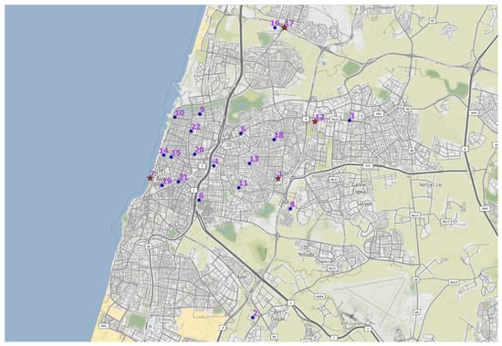
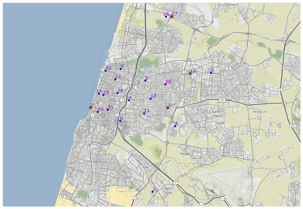
The data for the actual model application and validation was a dataset of a wind measurement campaign conducted in the metropolitan area of Tel Aviv, from 1 February 1998 to 30 June 1999. The campaign consisted of the deployment of 22 weather stations (Figure 1). All weather stations consisted of Young model 05103 wind monitor anemometers which measured wind speed and direction. Sensor accuracy was $\pm 0.3{\displaystyle \frac{\mathrm{m}}{\mathrm{s}}}$ for wind speed and $\pm 3°$ for wind direction. Measurements were made at a rate of 1 Hz [57]. These were collected by a Campbell Scientific CR10 data logger. The data logger internal programs were used to produce 10 min vectorial averages of the wind speed and direction [58]. These were stored on a Campbell Scientific SM 192 storage module [59]. The collected data was downloaded to a laptop computer once every two or three days.

Figure 1. The weather stations’ network in the metropolitan area of Tel Aviv, during the 1998-9 campaign.

Data quality control computer programs were applied on the data files, in order to remove erroneous records. The procedures included the search for characters in numeric fields, examination of the time order of records, and examination of whether the wind direction and speed were within the correct range, i.e., wind direction within $\left[0^{°},360°\right]$ and wind speed within $\left[0, 20 \mathrm{m}/\mathrm{s}\right]$. This maximal wind speed was set according to reported multiannual measurements in a representative station in Tel Aviv [60].

Most stations were mounted on 6 m masts on urban rooftops. Three stations were located in open rural areas on the outskirts of Tel Aviv. Of these, stations no. 2 and 16 were mounted on a mast of 10 m above ground, and station 17 was mounted on a 65 m mast. It should be noted that the metropolitan area of Tel Aviv is rather homogenous where typically the buildings are predominantly 3–4 stories, with a representative mean building height $H \approx 9-12 \mathrm{m}$ [11,13]. A 6 m mast on a typical Tel Aviv rooftop therefore places the anemometers at a total height of about 15–18 m, corresponding to roughly 1.5–2 times the mean building height. This configuration is consistent with the commonly used siting guideline of placing urban anemometers at least about 1.5 H above the mean roughness elements in areas of relatively uniform building height and density [39].

2.3. Application of the Statistical Model to the Tel Aviv Area

2.3.1. Sample Choice Considerations and Representativeness Examination

In order to apply the proposed statistical model, the complete 1998-9 metropolitan Tel Aviv dataset will be considered as the manifestation of the spatial populations of the wind vectors, $F_P$, at different time points. Therefore, $F_P$ for a given time point, t, say 1200 h in the summer season, consists of the available wind measurements that were collected in this time point in all days of the summer season.

The sample size was chosen in order to assure the invertibility of the sample covariance matrix, $S_t$, which is a key component in the tolerance region (Equation (3)) investigated in this study. This matrix is invertible when its dimension, $d$, is larger than the sample size, $n$ [61]. $S_t$ is a matrix of $2\times 2$ (Equation (2)), so d is 2 and n is 4. This satisfies the invertibility condition. The decision regarding the possible inclusion of weather stations in the sample $F_S$ was based on climatological considerations. Due to the fact that the morphology of the metropolitan area of Tel Aviv is rather homogenous, where the urban fabric is dominated by low-rise buildings, the flow in the Tel Aviv urban boundary layer (UBL) is adapted to the rough urban surface layer and is not disturbed by individual buildings [11,13,62,63]. The flow in the UBL also reflects processes that operate at larger scales, specifically the flow characteristic of the upwind rural surface [12,64]. The rural area surrounding Tel Aviv is the central coastal plain of Israel. The flow in this area is characterized by a typical diurnal flow pattern: the Mediterranean Sea breeze regime during the day characterized by strong westerly to north-westerly winds, a land winds regime during the night, governed by weak southerly to south-easterly winds and two change periods between these [65]. Therefore, five alternative sample sets of four stations were selected and subsequently subjected to statistical analysis. The stations included in each alternative sample followed a common thread in an effort to best describe the flow into the metropolitan area of Tel Aviv. Alternative A includes weather stations that are close to the perimeter of the urban area, in order to capture the entrance of any transient rural flow into the metropolitan area of Tel Aviv. Alternative B consists of stations located along a diagonal line that crosses the area from northwest to southeast, in order to capture both outside flows and the flow generated within the urban area. Alternatives C and D consists of stations located along a line which bisects the area from west to east. Alternative C is positioned along the area’s southern section, while Alternative D runs through its northern one. Alternative E consists of stations in central portion of the city of Tel Aviv, and tries to capture flows that originate within the urban area (Figure S1 in the Supplementary Material).

In order to examine the representativeness of the chosen sample, a comparison will be conducted. This will involve the comparison of the Mahalanobis distance distributions. For each wind vector observation in time t measured on a weather station in position $\left(x,y\right)$, the Mahalanobis distance was calculated by:

$${\mathit{D}}^2={\left({\mathit{U}}_{{\mathit{t}}_{\mathit{x},\mathit{y}}}-{\overline{\mathbf{U}}}_{\mathit{t}}\right)}^{\mathit{T}}{\mathit{S}}_{\mathit{t}}^{-1}\left({\mathit{U}}_{{\mathit{t}}_{\mathit{x},\mathit{y}}}-{\overline{\mathbf{U}}}_{\mathit{t}}\right)$$

(5)

This value was calculated both for the population and for the sample based on two different values of the spatial average, ${\stackrel{─}{\mathbf{U}}}_{\mathrm{t}}$, and the covariance matrix, ${\mathit{S}}_t$. For the population, $F_P$, $D^2$ was calculated for all weather stations, i.e., ${\mathit{U}}_{{\mathit{t}}_{\mathit{x},\mathit{y}}}\in F_P$ and for the sample, $F_S$, $D^2$ was calculated exclusively just for the weather stations included in the sample, ${\mathit{U}}_{{\mathit{t}}_{\mathit{x},\mathit{y}}}\in F_S$.

A comparison was conducted for the two main seasons, according to the seasons’ definition in the Eastern Mediterranean (EM) region [66], i.e., winter spans from December to March and Summer occurs between June and September.

2.3.2. Comparison of Empirical and Theoretical Mahalanobis Distance

For a list of arbitrary $D^2$ values, $E\left[p_i\right]=\tilde{P}$ was calculated for each of the combinations of season and time point. These were ${10}^{\beta }, \beta \in \left(-1, -0.75, -0.5, \dots , 1, 1.25, 1.5\right)$. Then, using the analytic expression in Equation (4), the value of P that leads to each of these $D^2$ values was calculated. For the comparison, four time points were chosen from each of the EM seasons. The time points were chosen to represent morning (0800 h), midday (1200 h), evening (2100 h) and night (0400 h) [29,65].

2.3.3. Estimation of the Mahalanobis Distance Function

Two empirical Mahalanobis distance functions were calculated, one for each of the main seasons in the EM, which are the summer and the winter. Each function was calculated based on three months of data, that is the learning dataset, thus leaving one month of data for the resultant model validation. The months that were used for validation are months which are considered high season, namely February for winter and August for summer [66]. Splitting data into disjoint learning (training) and validation (test) subsets is a standard practice in predictive modeling. The learning dataset is used to estimate the regression parameters, while the validation set provides an independent assessment of predictive performance [67,68].

The functions were estimated by first calculating the values of $E\left[p_i\right]=\tilde{P}$ that correspond to the list of arbitrary $D^2$ values that were described in the previous section. Then, the empirical Mahalanobis distance functions, $\tilde{P}\left(D^2\right)$, were fitted to these couples. In order to fit such functions, their functional form should be defined. When dealing with population tolerance, the logistic distribution is frequently used when the observations are not normally distributed. In order to do so, the expected proportions should be transformed into logits [69,70]:

$$\mathit{Y}=\mathit{l}\mathit{n}\left({\displaystyle \frac{\tilde{P}}{1-\tilde{P}}}\right)$$

(6)

This leads to the following functional form of the empirical $D^2$ functions:

$$\mathit{Y}=\mathit{l}\mathit{n}\left({\displaystyle \frac{\tilde{\mathit{P}}}{\mathbf{1}-\tilde{\mathit{P}}}}\right)=\mathit{a}+\mathit{b}·\mathit{l}\mathit{n}\left({\mathit{D}}^{\mathbf{2}}\right)$$

(7)

where the parameters of this log-logistic relationship can then be determined using linear regression [71].

The correlation coefficient, $R^2$, was used as a measure of the fit achieved by the linear regression. $R^2$ is the result of two sums of squares [72]. The first is the sum of squared deviations of the predictand, $\mathit{Y}$, from its mean, $\overline{\mathit{Y}}$:

$$SSD={\displaystyle \sum _{\mathit{i}=\mathbf{1}}^{\mathit{m}}}\left({\mathit{Y}}_{\mathit{i}}-\overline{\mathit{Y}}\right)$$

(8)

And the second is the sum of squared deviations from the prediction, $\widehat{\mathit{Y}}$:

$$SSP={\displaystyle \sum _{\mathit{i}=\mathbf{1}}^{\mathit{m}}}\left({\mathit{Y}}_{\mathit{i}}-{\widehat{\mathit{Y}}}_{\mathit{i}}\right)$$

(9)

where $m$ is the number of arbitrary $D^2$ values that were described earlier (Section 2.3.2).

Based on the two equations, $R^2$, is calculated:

$$R^2=\mathbf{1}-{\displaystyle \frac{SSP}{SSD}}$$

(10)

2.3.4. Model Validation

In order to validate the model, $E\left[p_i\right]=\tilde{P}$ was calculated for the list of arbitrary $D^2$ values, but in this case using the data of the months left for validation. The validation itself was made by comparing these results to the prediction interval, i.e., the confidence interval where future $\tilde{P}$ values should fall, given the log-logistic Mahalanobis distance functions that were previously calculated.

2.4. Extracting Wind Realizations

Given the sample average wind vector, ${\overline{\mathbf{U}}}_t$, the sample covariance matrix ${\mathit{S}}_t$ and empirical Mahalanobis distance function $D^2\left(\tilde{P}\right)$, then, for a specified proportion, $\tilde{P}$, it is possible to draw an ellipse, representing the tolerance region according to these variables’ values. In order to do so, ${\lambda }_1$ and ${\lambda }_2$, the eigenvalues of the matrix ${\mathit{S}}_t$ as well as the ellipse’s orientation, $\theta$, should be calculated as [56]:

$$\begin{gathered} {\lambda }_1={\displaystyle \frac{\mathit{var}\left({\mathit{u}}_{\mathit{t}}\right)+\mathit{var}\left({\mathit{v}}_{\mathit{t}}\right)}{2}}+\sqrt{{\left[{\displaystyle \frac{\mathit{var}\left({\mathit{u}}_{\mathit{t}}\right)-\mathit{var}\left({\mathit{v}}_{\mathit{t}}\right)}{2}}\right]}^2+{\left[\mathit{cov}\left({\mathit{u}}_{\mathit{t}},{\mathit{v}}_{\mathit{t}}\right)\right]}^2} \\ {\lambda }_2={\displaystyle \frac{\mathit{var}\left({\mathit{u}}_{\mathit{t}}\right)+\mathit{var}\left({\mathit{v}}_{\mathit{t}}\right)}{2}}-\sqrt{{\left[{\displaystyle \frac{\mathit{var}\left({\mathit{u}}_{\mathit{t}}\right)-\mathit{var}\left({\mathit{v}}_{\mathit{t}}\right)}{2}}\right]}^2+{\left[\mathit{cov}\left({\mathit{u}}_{\mathit{t}},{\mathit{v}}_{\mathit{t}}\right)\right]}^2} \\ \theta =\{\begin{array}{cc}0& if\mathit{cov}\left({\mathit{u}}_{\mathit{t}},{\mathit{v}}_{\mathit{t}}\right)=0 and\mathit{var}\left({\mathit{u}}_{\mathit{t}}\right)\ge \mathit{var}\left({\mathit{v}}_{\mathit{t}}\right)\\ 90°& if\mathit{cov}\left({\mathit{u}}_{\mathit{t}},{\mathit{v}}_{\mathit{t}}\right)=0 and\mathit{var}\left({\mathit{u}}_{\mathit{t}}\right)<\mathit{var}\left({\mathit{v}}_{\mathit{t}}\right)\\ atan2\left({\lambda }_1-\mathit{var}\left({\mathit{u}}_{\mathit{t}}\right),\mathit{cov}\left({\mathit{u}}_{\mathit{t}},{\mathit{v}}_{\mathit{t}}\right)\right)& otherwise\end{array} \end{gathered}$$

(11)

where atan2 is the 2-argument arctangent function.

Then, it is possible to calculate the coordinates of the elliptical tolerance region, which is a function of $\phi$, with an angle whose range is $\left[0°, 360°\right]$ around ${\stackrel{─}{\mathit{u}}}_{\mathit{t}}$ and ${\stackrel{─}{\mathit{v}}}_{\mathit{t}}$, the components of ${\overline{\mathbf{U}}}_t$:

$$\begin{gathered} x\left(\phi \right)={{\stackrel{─}{\mathit{u}}}_{\mathit{t}}+D}^2\left[{\lambda }_{2}cos\left(\theta \right)cos\left(\phi \right)-{\lambda }_{1}sin\left(\theta \right)sin\left(\phi \right)\right] \\ y\left(\phi \right)={{\stackrel{─}{\mathit{v}}}_{\mathit{t}}+D}^2\left[{\lambda }_{2}sin\left(\theta \right)cos\left(\phi \right)+{\lambda }_{1}cos\left(\theta \right)sin\left(\phi \right)\right] \end{gathered}$$

(12)

This equation represents the uncertainty as an elliptic-shaped statistical region tolerance region that contains a given expected proportion of the spatial wind vectors’ population. Now, by choosing some values of $\phi$, the possible values of the wind vector can be calculated from the above equation. As examples for this study, the following values were used: $\phi =\left\{0°, 90°, 180°, 270°\right\}$.

3. Results

3.1. Sample Representativeness Examination

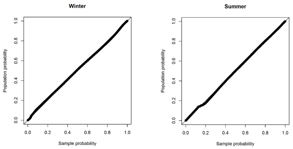
Of the five alternative samples, the chosen sample is Alternative A, which includes weather stations that are close to the perimeter of the urban area (Supplementary Material). These are: station number 7 in the southwest of the Tel Aviv metropolitan area, station number 1 in the southwest, number 12 in the east and number 17, the northernmost weather station in this area (Figure 1). The Mahalanobis distance distribution of this sample was compared to the equivalent distribution of the population. The comparison was made via probability–probability (P–P) plots. These plots are scatterplots of the cumulative probability of the population as a function of the cumulative probability of the sample. Each couple of population and sample probabilities corresponds to a common data value [56]. In this study, the data values that pair the sample and population probabilities are $D^2$ values, which were calculated for each of the seasons (Figure 2 and Figure S2 in the Supplementary Material).

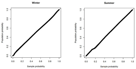
Figure 2. Comparison of seasonal sample (horizontal axis) and population (vertical axis) Mahalanobis distances—percentile–percentile (P–P) plot. The solid line is the line of equality.

All the points in all the seasonally P–P plots fall very close to the line of equality (Figure 2). Comparatively, the other alternative samples have exhibited a portion of the plot that is either above the line of equality (Figure S2B–D), or below it (Figure S2E). The maximal differences between alternative sample A and the population cumulative probabilities were 2% in the winter and 2.3% in the summer. The maximal differences between the other alternative samples and the population cumulative probabilities ranged from 4.5% (Alternative D) to 7.4% (Alternative B) in the winter, and from 3.9% (Alternative C) to 7.5% (Alternative E) in the summer. Because the maximal differences achieved by alternative sample A are considerably smaller than those of any other alternative, it clearly provides the best representation of the population.

3.2. Comparison Between the Empirical and Theoretical Mahalanobis Distance

The comparison involved the season and time of the day and was conducted using percentile–percentile (P–P) plots. These plots consist of pairs of proportions that relate to the same Mahalanobis distance, $D^2$. Each pair of proportions consists of an empirical $\tilde{P}$ and a theoretical $P$ calculated by inverting the analytic expression in Equation (4). The pairs relate to the arbitrary $D^2$ values that were described earlier (Section 2.3.2).

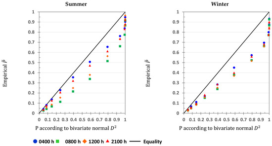
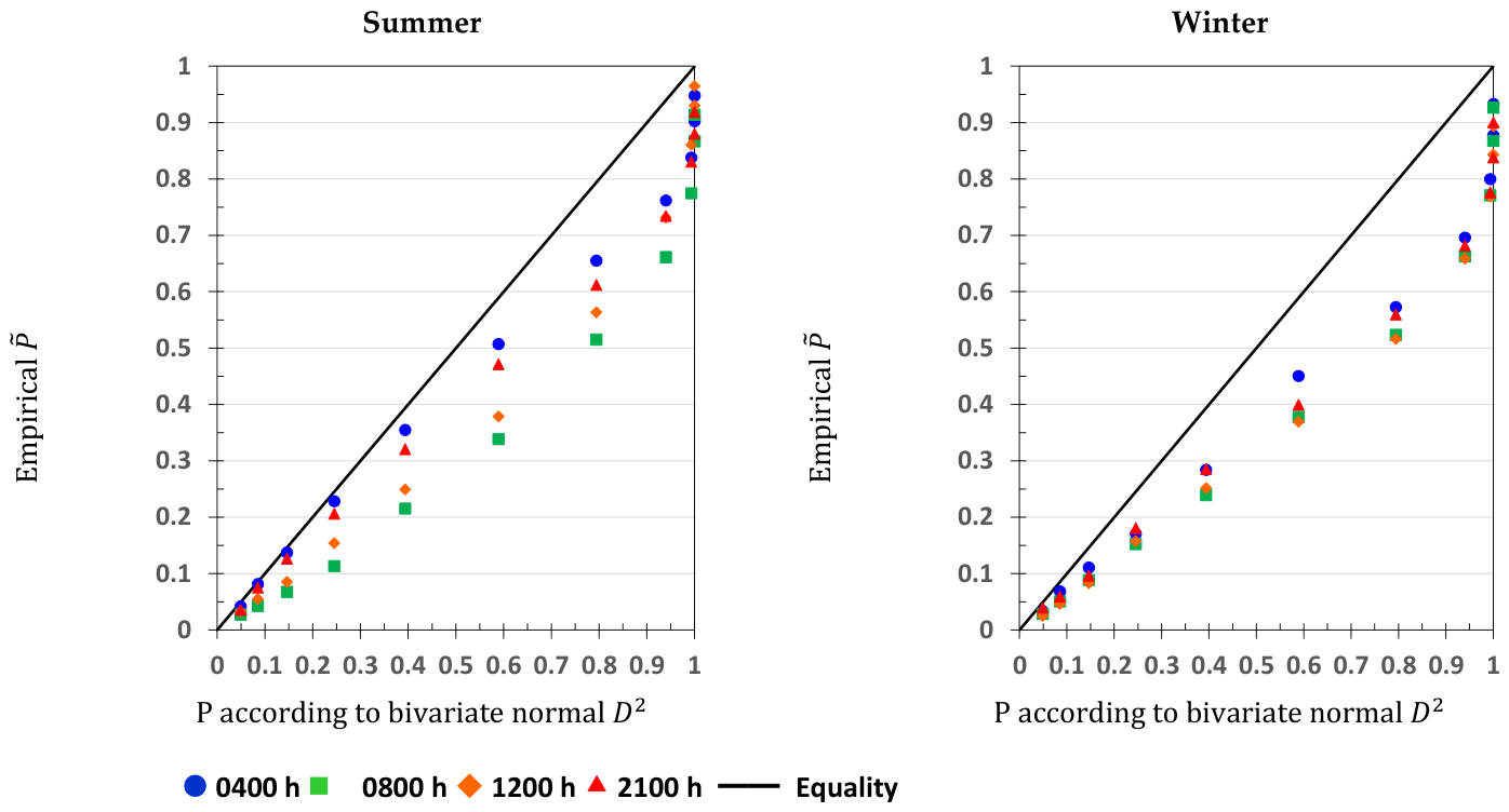
The comparison shows that all the points are to the right and below the equality line (Figure 3). This means that the empirical values do not exceed the theoretical ones. There are some cases in which the empirical $D^2$ values are close to the theoretical, such as proportions up to 40% during the evening (2100 h) and night (0400 h) of the summer season (Figure 3). However, in most cases the theoretical proportions are considerably larger than the empirical ones. This is evident during the winter season in all the examined time points, for theoretical proportions greater than 10%, and also during the day, at 0800 h and 1200 h in the summer (Figure 3).

Figure 3. A Percentile–Percentile (P–P) plot comparing pairs of theoretical P, according to the bivariate normal distribution’s $D^2$ function (horizontal axis) and empirical $\tilde{P}$ (vertical axis). P and $\tilde{P}$ are paired by the same $D^2$. The 4 kinds of dots refer to 4 time points during the summer (left) and winter (right) seasons. The solid line is the line of equality.

3.3. The Empirical Mahalanobis Distance Function

Due to the insufficient agreement between the empirical $D^2$ distribution and the theoretical Mahalanobis function according to the bivariate normal distribution, empirical Mahalanobis distance functions were established for each of the main seasons. As described earlier (Section 2.3.3) their functional form was based on a log-logistic relationship (Equation (7)) and their parameters were estimated using linear regression [71]. The resultant functions, when restated as $D^2\left(\tilde{P}\right)$ are:

$$\begin{array}{c}\begin{array}{cc}{\mathit{D}}^{\mathbf{2}}={\left({\displaystyle \frac{\tilde{\mathit{P}}}{\mathbf{1}-\tilde{\mathit{P}}}}·{\mathit{e}}^{\mathbf{0.9114}}\right)}^{{\displaystyle \frac{\mathbf{1}}{\mathbf{1.0905}}}}& \mathit{f}\mathit{o}\mathit{r} \mathit{s}\mathit{u}\mathit{m}\mathit{m}\mathit{e}\mathit{r}\\ {\mathit{D}}^{\mathbf{2}}={\left({\displaystyle \frac{\tilde{\mathit{P}}}{\mathbf{1}-\tilde{\mathit{P}}}}·{\mathit{e}}^{\mathbf{1.0635}}\right)}^{{\displaystyle \frac{\mathbf{1}}{\mathbf{1.0118}}}}& \mathit{f}\mathit{o}\mathit{r} \mathit{w}\mathit{i}\mathit{n}\mathit{t}\mathit{e}\mathit{r}\end{array}\\ \end{array}$$

(13)

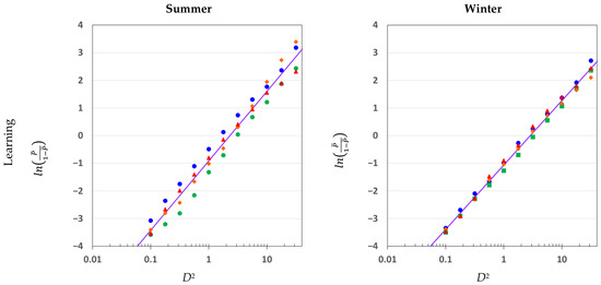
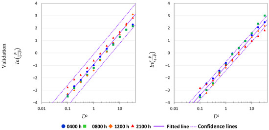
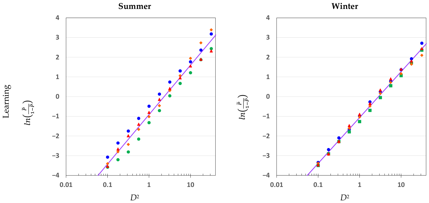
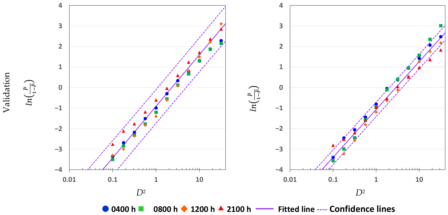
These functions resulted in $R^2$ values of 0.9735 for the summer and 0.9943 for the winter (Figure 4 top panels). All the values calculated for the summer validation data set fall within the upper and lower prediction interval of 99% (Figure 4, lower left panel). Regarding the winter validation data set, 77% of the values fall within the boundaries of the prediction interval (Figure 4, lower right panel). This percentage remains consistent throughout the diurnal cycle, with 82% at midday (1200 h) and night (0400 h), and 73% during the morning (0800 h) and evening (2100 h). The validation $R^2$ were 0.9753 for the summer and 0.9707 for the winter. The close agreement between the learning and validation $R^2$ indicates a robust regression fit, with no signs of overfitting.

Figure 4. The estimated empirical Mahalanobis distance functions $\mathit{l}\mathit{n}\left({\displaystyle \frac{\tilde{\mathit{P}}}{\mathbf{1}-\tilde{\mathit{P}}}}\right)=\mathit{f}\left(\mathit{l}\mathit{n}\left({\mathit{D}}^2\right)\right)$ for the summer and winter seasons (solid purple line), based on the learning dataset (top panels) and the comparison of these functions to the validation dataset (lower panels). The dashed lines signify upper and lower prediction intervals of 99%.

Now, for each $\tilde{P}$, which acts as the degree of spatial uncertainty, it is possible to receive a quantified uncertainty, as $D^2\left(\tilde{P}\right)$ defines the actual size of the tolerance region (Equation (5)).

4. Discussion and Summary

This study presents a method that quantifies the spatial uncertainty of the urban rooftop wind. It does so by describing this uncertainty as an elliptic-shaped statistical tolerance region that contains a given expected proportion of the spatial wind vectors’ population. This method deals with the problem of making a reliable statistical projection of the degree of heterogeneity of an urban region, based on real-time measurements of a sparse network of weather stations and a historic dataset of denser measurements. Such projection, expressed as a tolerance region for given proportions, can be obtained by the following steps:

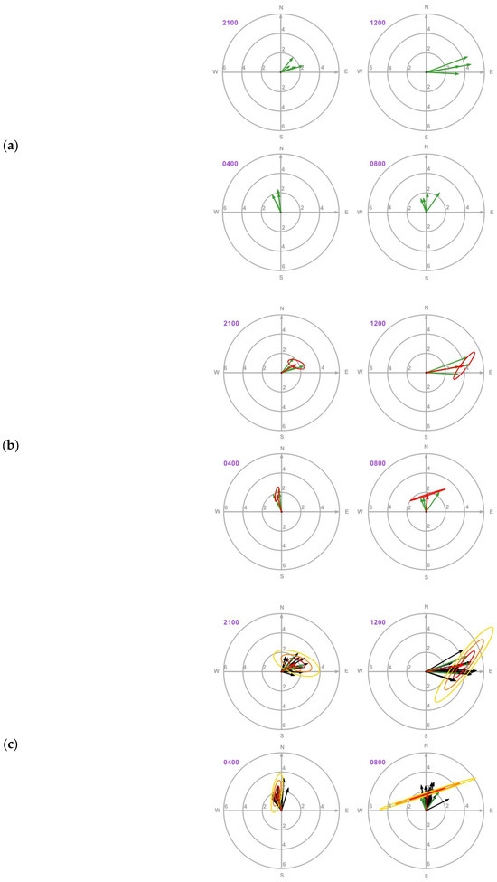
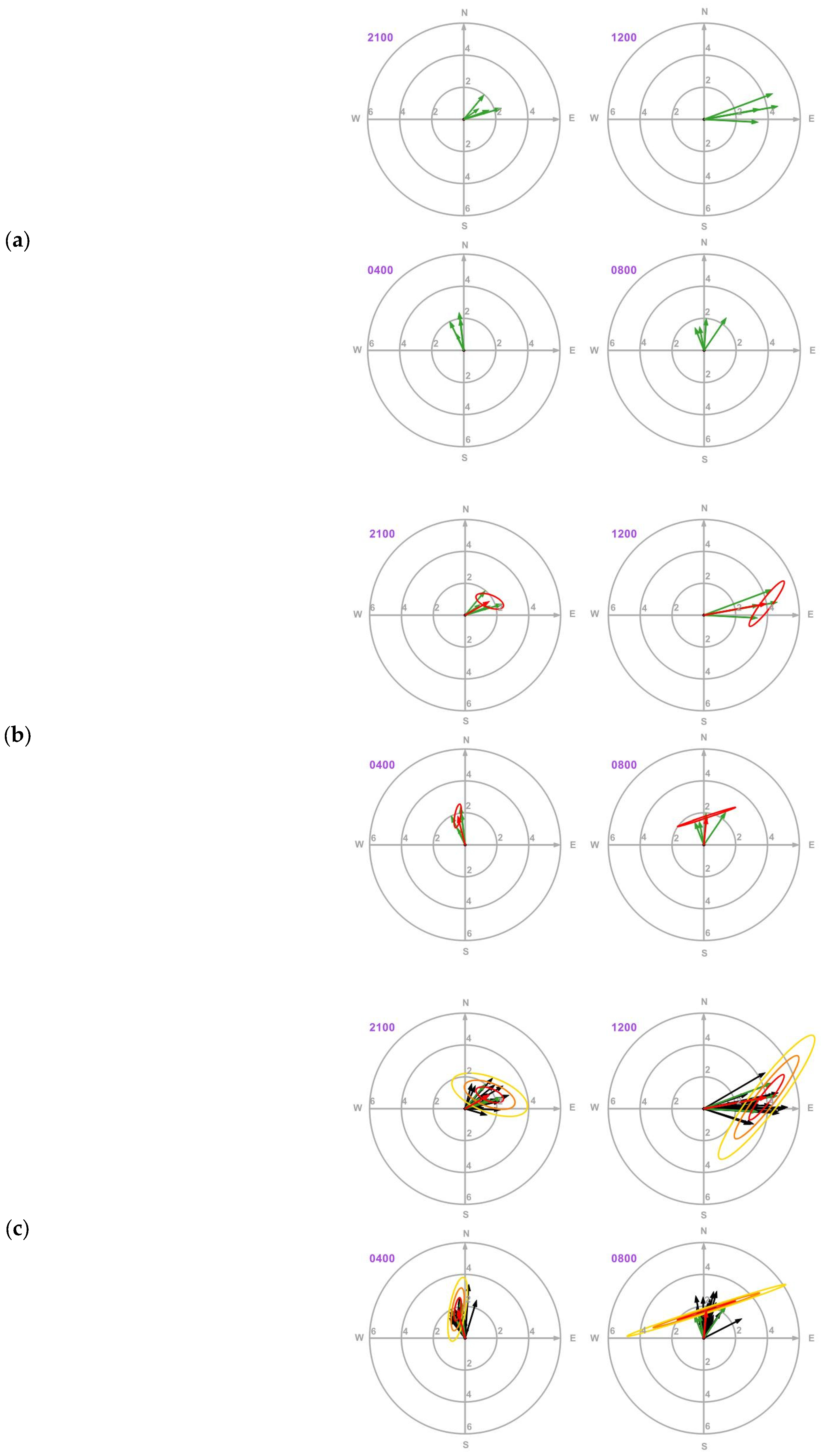
• Input of the current wind vector measured by a representative sample consisting of four weather stations. This is exemplified for several time points in a typical day in Tel-Aviv (Figure 5a).
  

  Figure 5. The steps in obtaining a statistical projection using the model, exemplified for several time points (2100 h, 1200 h, 0400 h, 0800 h) on 15 August 1998: input from the sample weather stations (panel (a), green arrows); sample’s average and covariance matrix (panel (b), red arrows and ellipse); tolerance regions for given proportions (panel (c), red, orange and yellow ellipses for proportions of 50%, 66%, 75% respectively). For comparison, all available wind vectors measured on these time points appear as well (panel (c), black arrows). The tips of the arrows point towards the wind’s destination. The Cartesian axis (in gray) shows the cardinal directions and the circles (also in gray) show the speed (in m/s, by steps of 2 m/s).
• Calculation of the sample’s average and covariance matrix (Figure 5b).
• For given proportions, Mahalanobis distance values are obtained from the log-logistic empirical functions (Equation (13)). These are based on a historic dataset of dense network of weather stations.
• Elliptical tolerance regions are provided, which are defined by the sample’s average, covariance matrix and the Mahalanobis distances (Equations (11) and (12)). Each of these ellipses contains a proportion of the wind vectors expected in the area (Figure 5c).

An example of the implementation of these steps by using a simple code in R (version 4.1.1; R Core Team, 2021) is detailed in the Supplementary Material (Figure S3 and the associated text). The run time of this code is less than 1 s on a regular PC.

This study has shown that a sample of four weather stations can accurately represent a population of urban spatial wind vectors. The application and validation were performed on a dataset collected from a weather stations’ network in metropolitan Tel-Aviv which consisted of 22 wind observation stations. This network size is comparable in size to the 28-station network in Birmingham [73] and the 24-station network in Amsterdam [32]. It is larger than the networks in Berlin [31] and in Ghent [33] which consist of 10 and 6 wind observation stations, respectively. Because Tel Aviv’s weather station network is comparable in scale to larger urban networks, it can accurately characterize the wind vectors’ population.

This representativeness of such a small sample is interesting because many statistical applications consider such a sample as very small [74,75,76]. Moreover, a key component in the tolerance region investigated in this study is the sample covariance matrix. Such covariance matrix is invertible when its dimension, $d$, is larger than the sample size, $n$. For a sample size of $n$ independent observations, it is also required that the ratio $d/n$ should be negligible [61]. In this study, the covariance matrix is $2\times 2$, so d is 2 and n is 4. This satisfies the invertibility condition, but not the ratio requirement. A possible explanation for this small sample size is that it is usually assumed that the samples drawn from a population are statistically independent. An assumption of such independence cannot be valid when dealing with weather stations situated in a given region, because most of the time all these stations are influenced by common larger scale meteorological phenomena. The role of dependency can be exemplified by the Chebyshev inequality for bivariate random variables [77,78]:

$$\begin{array}{c}Pr\left({\left({\mathit{U}}_{{\mathit{t}}_{\mathit{x},\mathit{y}}}-{\overline{\mathbf{U}}}_{\mathit{t}}\right)}^{\mathit{T}}{\mathit{S}}_{\mathit{t}}^{-\mathbf{1}}\left({\mathit{U}}_{{\mathit{t}}_{\mathit{x},\mathit{y}}}-{\overline{\mathbf{U}}}_{\mathit{t}}\right)<D^2\right)\ge \mathbf{1}-{\displaystyle \frac{\mathbf{2}}{D^2}}\\ \end{array}$$

(14)

According to this inequality, for any underlying bivariate distribution it can be guaranteed that an ellipse tolerance region will contain at least $100\left(1-{\displaystyle \frac{2}{D^2}}\right)\%$ of the wind vectors’ population for all $D^2\ge 2$ [77,78]. For example, using Equation (10), for $\tilde{P}=0.66$, $D^2$ equals 4.238 for the summer season and 5.51 for the winter. For these $D^2$ values, the Chebyshev inequality guarantees that $\tilde{P}$ is greater than 0.53 and 0.64. The correlation coefficient, $\mathsf{\rho }$, can be calculated by the components of the covariance matrix, $S_t$, as $\mathsf{\rho }={\displaystyle \frac{cov\left(u_t,v_t\right)}{\sqrt{var\left(u_t\right)\backslash bulletvar\left(v_t\right)}}}\in \left(-\mathrm{1,1}\right)$. Thus, the Chebyshev inequality can be alternatively formulated in terms of the correlation coefficient, $\mathsf{\rho }$:

$$Pr\left({\left[{\displaystyle \frac{\left(u_t-{\overline{u}}_t\right)}{\sqrt{var\left(u_t\right)}}}-{\displaystyle \frac{\left(v_t-{\overline{v}}_t\right)}{\sqrt{var\left(v_t\right)}}}\right]}^2+2\left(1-\rho \right){\displaystyle \frac{\left(u_t-{\overline{u}}_t\right)}{\sqrt{var\left(u_t\right)}}}{\displaystyle \frac{\left(v_t-{\overline{v}}_t\right)}{\sqrt{var\left(v_t\right)}}}<D^2\right)\ge 1-2{\displaystyle \frac{1-{\rho }^2}{D^2}}$$

(15)

This formulation is valid for all $D^2\ge 2\left(1-{\mathsf{\rho }}^2\right)$, provided $D^2\ne 0$. This expression quantifies the contribution of the weather stations’ dependence, showing that as the correlation strengthens, the minimal guaranteed proportion rises accordingly. Supposedly, if the right-hand side of the inequality would be equal to 0.66, then the $D^2$ values mentioned earlier, 4.238 for the summer season and 5.51 for the winter, correspond to absolute correlation values of 0.529 and 0.252 for summer and winter, respectively. Therefore, as some degree of dependency can be expected in an urban wind field, this population can be represented by a smaller sample than the one required when it is assumed that the population is composed of independent random variables.

The results of the comparison between the samples’ empirical $D^2$ distribution and the theoretical one according to the bivariate normal distribution has shown that the empirical values are either smaller than the empirical ones, or at most similar. This suggests that the empirical Mahalanobis distance distributions are either narrower than the theoretical distribution or similar to it. Therefore, the theoretical bivariate normal Mahalanobis distance function can be considered as somewhat of upper limit to the empirical one.

It was found that a single seasonal Mahalanobis distance function can fit well with the data, along all the flow patterns during the day. These results suggest that although the spatial average and covariance matrix changes along the day, the functional form of the distribution is fairly constant throughout the season. The fact that the seasonal Mahalanobis distance functions were appropriate for the validation data suggest that these functions, alongside a calculation of the real-time sample mean and covariance matrix, can serve as a statistical model for the urban wind field, as exemplified for the Tel Aviv area. Such a model provides an elliptic-shaped tolerance region that contains a given expected proportion of the spatial wind vectors’ population.

The statistical model in this study was demonstrated on the metropolitan area of Tel Aviv. The analysis-based methodology presented in this study addresses the horizontally homogeneous inertial sub-layer which is the layer just above the canopy roughness sub-layer. It is therefore expected to perform well in other cities with a well-defined inertial sub-layer. This is consistent with previous generalizations of inertial sub-layer wind vector fields, such as turbulent standard deviations [1].

However, the choice of configuration and size of the sample should be carefully analyzed for each individual city, due to site-specific topographical and morphological features as well as the variability of diurnal larger scale flow. A useful rule of thumb is to examine the spatial correlation which indicates weather stations’ redundancy. This suggests a possible reduction in the sample size required to achieve a statistical representation of the wind vector population.

References

- Roth, M. Review of Atmospheric Turbulence over Cities. Q. J. R. Meteorol. Soc. 2000, 126, 941–990. [Google Scholar] [CrossRef] [Scilit]
- Shraiman, B.I.; Siggia, E.D. Scalar Turbulence. Nature 2000, 405, 639–646. [Google Scholar] [CrossRef] [Scilit] [PubMed]
- Li, D.; Bou-Zeid, E. Coherent Structures and the Dissimilarity of Turbulent Transport of Momentum and Scalars in the Unstable Atmospheric Surface Layer. Bound.-Layer Meteorol. 2011, 140, 243–262. [Google Scholar] [CrossRef] [Scilit]
- Stull, R.B. An Introduction to Boundary Layer Meteorology; Stull, R.B., Ed.; Springer: Dordrecht, The Netherlands, 1988; ISBN 978-90-277-2769-5. [Google Scholar]
- Stockie, J.M. The Mathematics of Atmospheric Dispersion Modeling. Siam Rev. 2011, 53, 349–372. [Google Scholar] [CrossRef] [Scilit]
- Jänhall, S. Review on Urban Vegetation and Particle Air Pollution—Deposition and Dispersion. Atmos. Environ. 2015, 105, 130–137. [Google Scholar] [CrossRef] [Scilit]
- Tritscher, T.; Raz, R.; Levi, Y.; Levy, I.; Broday, D.M. Emissions vs. Turbulence and Atmospheric Stability: A Study of Their Relative Importance in Determining Air Pollutant Concentrations. Sci. Total Environ. 2020, 733, 139300. [Google Scholar] [CrossRef] [Scilit] [PubMed]
- Fattal, E.; David-Saroussi, H.; Klausner, Z.; Buchman, O. An Urban Lagrangian Stochastic Dispersion Model for Simulating Traffic Particulate-Matter Concentration Fields. Atmosphere 2021, 12, 580. [Google Scholar] [CrossRef] [Scilit]
- Fattal, E.; David-Saroussi, H.; Buchman, O.; Tas, E.; Klausner, Z. Heterogenous Canopy in a Lagrangian-Stochastic Dispersion Model for Particulate Matter from Multiple Sources over the Haifa Bay Area. Atmosphere 2023, 14, 144. [Google Scholar] [CrossRef] [Scilit]
- Mittal, H.; Sharma, A.; Gairola, A. A Review on the Study of Urban Wind at the Pedestrian Level around Buildings. J. Build. Eng. 2018, 18, 154–163. [Google Scholar] [CrossRef] [Scilit] [PubMed]
- Saaroni, H.; Ben-Dor, E.; Bitan, A.; Potchter, O. Spatial Distribution and Microscale Characteristics of the Urban Heat Island in Tel-Aviv. Landsc. Urban Plan. 2000, 48, 1–18. [Google Scholar] [CrossRef] [Scilit]
- Collier, C.G. The Impact of Urban Areas on Weather. Q. J. R. Meteorol. Soc. 2006, 132, 1–25. [Google Scholar] [CrossRef] [Scilit]
- Shashua-Bar, L.; Potchter, O.; Bitan, A.; Boltansky, D.; Yaakov, Y. Microclimate Modelling of Street Tree Species Effects within the Varied Urban Morphology in the Mediterranean City of Tel Aviv, Israel. Int. J. Climatol. 2010, 30, 44–57. [Google Scholar] [CrossRef] [Scilit]
- van Hove, L.W.A.; Jacobs, C.M.J.; Heusinkveld, B.G.; Elbers, J.A.; Van Driel, B.L.; Holtslag, A.A.M. Temporal and Spatial Variability of Urban Heat Island and Thermal Comfort within the Rotterdam Agglomeration. Build. Environ. 2015, 83, 91–103. [Google Scholar] [CrossRef] [Scilit]
- Schmitt, A.U.; Burgemeister, F.; Dorff, H.; Finn, T.; Hansen, A.; Kirsch, B.; Lange, I.; Radtke, J.; Ament, F. Assessing the Weather Conditions for Urban Cyclists by Spatially Dense Measurements with an Agent-based Approach. Meteorol. Appl. 2023, 30, e2164. [Google Scholar] [CrossRef] [Scilit]
- Kothari, M.; Postlethwaite, I.; Gu, D.W. Uav Path Following in Windy Urban Environments. J. Intell. Robot. Syst. Theory Appl. 2014, 74, 1013–1028. [Google Scholar] [CrossRef] [Scilit]
- Patrikar, J.; Moon, B.G.; Scherer, S. Wind and the City: Utilizing UAV-Based In-Situ Measurements for Estimating Urban Wind Fields. In Proceedings of the 2020 IEEE/RSJ International Conference on Intelligent Robots and Systems (IROS); IEEE: Las Vegas, NV, USA, 2020; pp. 1254–1260. [Google Scholar]
- Veiga-Piñeiro, G.; Aldao-Pensado, E.; Martín-Ortega, E. Hybrid CFD-Deep Learning Approach for Urban Wind Flow Predictions and Risk-Aware UAV Path Planning. Drones 2025, 9, 791. [Google Scholar] [CrossRef] [Scilit]
- Katsoulis, B.D.; Theoharatos, G.A. Indications of the Urban Heat Island in Athens, Greece. J. Clim. Appl. Meteorol. 1985, 24, 1296–1302. [Google Scholar] [PubMed]
- Mestayer, P.G.; Durand, P.; Augustin, P.; Bastin, S.; Bonnefond, J.M.; Bénech, B.; Campistron, B.; Coppalle, A.; Delbarre, H.; Dousset, B.; et al. The Urban Boundary-Layer Field Campaign in Marseille (UBL/CLU-ESCOMPTE): Set-up and First Results. Bound.-Layer Meteorol. 2005, 114, 315–365. [Google Scholar] [CrossRef] [Scilit]
- Emmanuel, I.; Andrieu, H.; Leblois, E.; Flahaut, B. Temporal and Spatial Variability of Rainfall at the Urban Hydrological Scale. J. Hydrol. 2012, 430–431, 162–172. [Google Scholar] [CrossRef] [Scilit]
- Heusinkveld, B.G.; Steeneveld, G.J.; van Hovel, L.W.A.; Jacobs, C.M.J.; Holtslag, A.A.M. Spatial Variability of the Rotterdam Urban Heat Island as Influenced by Urban Land Use. J. Geophys. Res. Atmos. 2014, 119, 677–692. [Google Scholar] [CrossRef] [Scilit]
- Hanna, S.R.; Brown, M.J.; Camelli, F.E.; Chan, S.T.; Coirier, W.J.; Hansen, O.R.; Huber, A.H.; Kim, S.; Reynolds, R.M. Detailed Simulations of Atmospheric Flow and Dispersion in Downtown Manhattan: An Application of Five Computational Fluid Dynamics Models. Bull. Am. Meteorol. Soc. 2006, 87, 1713–1726. [Google Scholar] [CrossRef] [Scilit]
- Liu, Z.; Chen, Y.; Wang, Y.; Liu, C.; Liu, S.; Liao, H. The Development and Validation of the Inhomogeneous Wind Scheme for Urban Street (IWSUS-V1). Geosci. Model Dev. 2023, 16, 4385–4403. [Google Scholar] [CrossRef] [Scilit]
- Karthikeya, B.R.; Negi, P.S.; Srikanth, N. Wind Resource Assessment for Urban Renewable Energy Application in Singapore. Renew. Energy 2016, 87, 403–414. [Google Scholar] [CrossRef] [Scilit]
- Hanna, S.; Chang, J. Acceptance Criteria for Urban Dispersion Model Evaluation. Meteorol. Atmos. Phys. 2012, 116, 133–146. [Google Scholar] [CrossRef] [Scilit]
- Muller, C.L.; Chapman, L.; Grimmond, C.S.B.; Young, D.T.; Cai, X. Sensors and the City: A Review of Urban Meteorological Networks. Int. J. Climatol. 2013, 33, 1585–1600. [Google Scholar] [CrossRef] [Scilit]
- Wise, D.J.; Boppana, V.B.L.; Li, K.W.; Poh, H.J. Effects of Minor Changes in the Mean Inlet Wind Direction on Urban Flow Simulations. Sustain. Cities Soc. 2018, 37, 492–500. [Google Scholar] [CrossRef] [Scilit]
- Klausner, Z.; Ben-Efraim, M.; Arav, Y.; Tas, E.; Fattal, E. The Micrometeorology of the Haifa Bay Area and Mount Carmel during the Summer. Atmosphere 2021, 12, 354. [Google Scholar] [CrossRef] [Scilit]
- Chapman, L.; Muller, C.L.; Young, D.T.; Warren, E.L.; Grimmond, C.S.B.; Cai, X.M.; Ferranti, E.J.S. The Birmingham Urban Climate Laboratory: An Open Meteorological Test Bed and Challenges of the Smart City. Bull. Am. Meteorol. Soc. 2015, 96, 1545–1560. [Google Scholar] [CrossRef] [Scilit]
- Ebert, C.; Meier, F.; Weiss, J. Linear and POD-Based Interpolation of Simulated Urban Wind Fields with Experimental Validation. J. Wind Eng. Ind. Aerodyn. 2026, 274, 106468. [Google Scholar] [CrossRef] [Scilit]
- Ronda, R.J.; Steeneveld, G.J.; Heusinkveld, B.G.; Attema, J.J.; Holtslag, A.A.M. Urban Finescale Forecasting Reveals Weather Conditions with Unprecedented Detail. Bull. Am. Meteorol. Soc. 2017, 98, 2675–2688. [Google Scholar] [CrossRef] [Scilit]
- Caluwaerts, S.; Hamdi, R.; Top, S.; Lauwaet, D.; Berckmans, J.; Degrauwe, D.; Dejonghe, H.; De Ridder, K.; De Troch, R.; Duchêne, F.; et al. The Urban Climate of Ghent, Belgium: A Case Study Combining a High-Accuracy Monitoring Network with Numerical Simulations. Urban Clim. 2020, 31, 100565. [Google Scholar] [CrossRef] [Scilit]
- Droste, A.M.; Heusinkveld, B.G.; Fenner, D.; Steeneveld, G.J. Assessing the Potential and Application of Crowdsourced Urban Wind Data. Q. J. R. Meteorol. Soc. 2020, 146, 2671–2688. [Google Scholar] [CrossRef] [Scilit]
- Zhao, W.; Zhong, Y.; Li, Q.; Li, M.; Liu, J.; Tang, L. Comparison and Correction of IDW Based Wind Speed Interpolation Methods in Urbanized Shenzhen. Front. Earth Sci. 2022, 16, 798–808. [Google Scholar] [CrossRef] [Scilit]
- Kakavitsas, N.P.; Uddin, M.; Wolek, A. Mapping Urban Wind Fields via Gaussian Processes Regression Models That Consider Building Morphology. In Proceedings of the AIAA SCITECH 2025 Forum, Orlando, FL, USA, 6 January 2025; American Institute of Aeronautics and Astronautics: Reston, VA, USA, 2025. [Google Scholar]
- Lumet, E.; Rochoux, M.C.; Jaravel, T.; Lacroix, S. Uncertainty-Aware Surrogate Modeling for Urban Air Pollutant Dispersion Prediction. Build. Environ. 2025, 267, 112287. [Google Scholar] [CrossRef] [Scilit]
- BenMoshe, N.; Fattal, E.; Leitl, B.; Arav, Y. Using Machine Learning to Predict Wind Flow in Urban Areas. Atmosphere 2023, 14, 990. [Google Scholar] [CrossRef] [Scilit]
- Oke, T.R. Initial Guidance to Obtain Representative Meteorological Observations at Urban Sites; World Meteorological Organization: Geneva, Switzerland, 2006; Volume 81. [Google Scholar]
- Hanna, S.; White, J.; Zhou, Y. Observed Winds, Turbulence, and Dispersion in Built-up Downtown Areas of Oklahoma City and Manhattan. Bound.-Layer Meteorol. 2007, 125, 441–468. [Google Scholar] [CrossRef] [Scilit]
- Macdonald, R.W.; Griffiths, R.F.; Hall, D.J. An Improved Method for the Estimation of Surface Roughness of Obstacle Arrays. Atmos. Environ. 1998, 32, 1857–1864. [Google Scholar] [CrossRef] [Scilit]
- Grimmond, C.S.B.; Oke, T.R. Aerodynamic Properties of Urban Areas Derived from Analysis of Surface Form. J. Appl. Meteorol. Climatol. 1999, 38, 1262–1292. [Google Scholar] [CrossRef] [Scilit]
- Kastner-Klein, P.; Rotach, M.W. Mean Flow and Turbulence Characteristics in an Urban Roughness Sublayer. Bound.-Layer Meteorol. 2004, 111, 55–84. [Google Scholar] [CrossRef] [Scilit]
- Hanna, S.R.; Britter, R.E. Wind Flow and Vapor Cloud Dispersion at Industrial and Urban Sites; Center for Chemical Process Safety/AIChE: New York, NY, USA, 2002; ISBN 0-8169-0863-X. [Google Scholar]
- Cheng, H.; Hayden, P.; Robins, A.G.; Castro, I.P. Flow over Cube Arrays of Different Packing Densities. J. Wind Eng. Ind. Aerodyn. 2007, 95, 715–740. [Google Scholar] [CrossRef] [Scilit]
- Dabberdt, W.F.; Miller, E. Uncertainty, Ensembles and Air Quality Dispersion Modeling: Applications and Challenges. Atmos. Environ. 2000, 34, 4667–4673. [Google Scholar] [CrossRef] [Scilit]
- Hanna, S.R. Chapter 4.0 A Review of Uncertainty and Sensitivity Analyses of Atmospheric Transport and Dispersion Models. Dev. Environ. Sci. 2007, 6, 331–351. [Google Scholar] [CrossRef] [Scilit]
- Kolczynski, W.C.; Stauffer, D.R.; Haupt, S.E.; Deng, A. Ensemble Variance Calibration for Representing Meteorological Uncertainty for Atmospheric Transport and Dispersion Modeling. J. Appl. Meteorol. Climatol. 2009, 48, 2001–2021. [Google Scholar] [CrossRef] [Scilit]
- Klausner, Z.; Fattal, E. A New Theoretical Framework for Modeling Respiratory Protection Based on the Beta Distribution. Ann. Occup. Hyg. 2014, 58, 912–920. [Google Scholar] [CrossRef] [Scilit] [PubMed]
- Klausner, Z.; Fattal, E. An Ab Initio Approach for Modeling Respirator Penetration Distribution. In Handbook of Respiratory Protection: Safeguarding Against Current and Emerging Hazards; Racz, L., Yamamoto, D.P., Eninger, R.M., Eds.; CRC Press: Boca Raton, FL, USA, 2018; pp. 485–499. ISBN 9781498781145. [Google Scholar]
- Gavze, E.; Fattal, E. A Semi-Analytical Model for Short-Range Near-Ground Continuous Dispersion. Bound.-Layer Meteorol. 2018, 169, 297–326. [Google Scholar] [CrossRef] [Scilit]
- Oke, T.R. Methods in Urban Climatology. In Applied Climatology; Kirchhofer, W., Ohmura, A., Wanner, H., Eds.; ETH—Geographisches Institut Eidgenossische Technische Hochschule Zurich: Zurich, Switzerland, 1984. [Google Scholar]
- Muller, C.L.; Chapman, L.; Grimmond, C.S.B.; Young, D.T.; Cai, X.-M. Toward a Standardized Metadata Protocol for Urban Meteorological Networks. Bull. Am. Meteorol. Soc. 2013, 94, 1161–1185. [Google Scholar] [CrossRef] [Scilit]
- Klausner, Z.; Kaplan, H.; Fattal, E. The Similar Days Method for Predicting near Surface Wind Vectors. Meteorol. Appl. 2009, 16, 569–579. [Google Scholar] [CrossRef] [Scilit]
- Chew, V. Confidence, Prediction, and Tolerance Regions for the Multivariate Normal Distribution. J. Am. Stat. Assoc. 1966, 61, 605. [Google Scholar] [CrossRef] [Scilit]
- Wilks, D.S. Statistical Methods in the Atmospheric Sciences, 3rd ed.; Academic Press: Oxford, UK, 2011; Volume 100, ISBN 9780123850225. [Google Scholar]
- R.M. Young Company. Instructions Manual—Wind Monitor Model 05103. Available online: https://www.youngusa.com/wp-content/uploads/2021/02/05103-90N.pdf (accessed on 2 May 2019).
- Campbell, S. Cr1O Measurement and Control Module Operator’ S Manual. Available online: https://s.campbellsci.com/documents/us/manuals/cr10.pdf (accessed on 2 May 2019).
- Campbell, S. Sm192/716 Storage Module Instruction Manual. Available online: https://s.campbellsci.com/documents/us/manuals/sm192716.pdf (accessed on 2 May 2019).
- Bitan, A.; Rubin, S. Climatic Atlas of Israel for Physical and Environmental Planning and Design; Ramot Publishing—Tel Aviv University: Tel Aviv, Israel, 1991. [Google Scholar]
- Ledoit, O.; Wolf, M. A Well-Conditioned Estimator for Large-Dimensional Covariance Matrices. J. Multivar. Anal. 2004, 88, 365–411. [Google Scholar] [CrossRef] [Scilit]
- Pearlmutter, D.; Berliner, P.; Shaviv, E. Evaluation of Urban Surface Energy Fluxes Using an Open-Air Scale Model. J. Appl. Meteorol. 2005, 44, 532–545. [Google Scholar] [CrossRef] [Scilit]
- Kayatekin, C. Missing Teeth and Sticky Parts of Urban Plans: The Case of Patrick Geddes’ Tel Aviv. Environ. Sci. Sustain. Dev. 2025, 10, 28–42. [Google Scholar] [CrossRef] [Scilit]
- Arnfield, A.J. Two Decades of Urban Climate Research: A Review of Turbulence, Exchanges of Energy and Water, and the Urban Heat Island. Int. J. Climatol. 2003, 23, 1–26. [Google Scholar] [CrossRef] [Scilit]
- Klausner, Z.; Fattal, E. An Objective and Automatic Method for Identification of Pattern Changes in Wind Direction Time Series. Int. J. Climatol. 2011, 31, 783–790. [Google Scholar] [CrossRef] [Scilit]
- Alpert, P.; Osetinsky, I.; Ziv, B.; Shafir, H. A New Seasons Definition Based on Classified Daily Synoptic Systems: An Example for the Eastern Mediterranean. Int. J. Climatol. 2004, 24, 1013–1021. [Google Scholar] [CrossRef] [Scilit]
- Kuhn, M.; Johnson, K. Applied Predictive Modeling; Springer: New York, NY, USA, 2013; ISBN 978-1-4614-6848-6. [Google Scholar]
- Ghojogh, B.; Crowley, M. The Theory Behind Overfitting, Cross Validation, Regularization, Bagging, and Boosting: Tutorial. arXiv 2023. [Google Scholar] [CrossRef] [Scilit]
- Johnson, N.L.; Kotz, S. Distributions in Statistics: Continous Univariate Distributions—2; John Wiley and Sons: New York, NY, USA, 1970; ISSN ISBN 0471446270. [Google Scholar]
- Finney, D.J. Statistical Method in Biological Assay, 2nd ed.; Charles Griffin & Company Limited: London, UK, 1964. [Google Scholar]
- Zar, J. Biostatistical Analysis, 5th ed.; Pearson Education Limited: Harlow, UK, 2014; ISBN 1-292-02404-6. [Google Scholar]
- Hawkins, D.M. The Problem of Overfitting. J. Chem. Inf. Comput. Sci. 2004, 44, 1–12. [Google Scholar] [CrossRef] [Scilit] [PubMed]
- Warren, E.L.; Young, D.T.; Chapman, L.; Muller, C.; Grimmond, C.S.B.; Cai, X.M. The Birmingham Urban Climate Laboratory–A High Density, Urban Meteorological Dataset, from 2012–2014. Sci. Data 2016, 3, 160038. [Google Scholar] [CrossRef] [Scilit] [PubMed]
- Button, K.S.; Ioannidis, J.P.A.; Mokrysz, C.; Nosek, B.A.; Flint, J.; Robinson, E.S.J.; Munafò, M.R. Power Failure: Why Small Sample Size Undermines the Reliability of Neuroscience. Nat. Rev. Neurosci. 2013, 14, 365–376. [Google Scholar] [CrossRef] [Scilit] [PubMed]
- Doswell, C. Small Sample Size and Data Quality Issues Illustrated Using Tornado Occurrence Data. E-J. Sev. Storms Meteorol. 2007, 2, 1–16. [Google Scholar] [CrossRef] [Scilit]
- Whitley, E.; Ball, J.; Moher, D.; Dulberg, C.; Wells, G.; Machin, D.; Campbell, M.; Fayers, P.; Pinol, A.; Rivers, E.; et al. Statistics Review 4: Sample Size Calculations. Crit. Care 2002, 6, 335. [Google Scholar] [CrossRef] [Scilit] [PubMed]
- Navarro, J. A Very Simple Proof of the Multivariate Chebyshev’s Inequality. Commun. Stat. Theory Methods 2016, 45, 3458–3463. [Google Scholar] [CrossRef] [Scilit]
- Navarro, J. A Note on Confidence Regions Based on the Bivariate Chebyshev Inequality. Applications to Order Statistics and Data Sets. Istat. J. Turk. Stat. Assoc. 2014, 7, 1–14. [Google Scholar]
Disclaimer/Publisher’s Note: The statements, opinions and data contained in all publications are solely those of the individual author(s) and contributor(s) and not of MDPI and/or the editor(s). MDPI and/or the editor(s) disclaim responsibility for any injury to people or property resulting from any ideas, methods, instructions or products referred to in the content. |
© 2026 by the authors. Licensee MDPI, Basel, Switzerland. This article is an open access article distributed under the terms and conditions of the Creative Commons Attribution (CC BY) license.