


Abstract
Accurate, high-resolution emission inventories are essential for air quality modeling and policy evaluation, yet national-scale inventories for Thailand remain limited in spatial and temporal detail. This study develops a comprehensive national emission inventory for Thailand in 2019 (EI–TH 2019), covering 12 major air pollutants and greenhouse gases across key sectors, including energy, transport, industry, agriculture, waste, and residential activities. The inventory is constructed using country-specific activity data from official statistics and sectoral surveys, combined with GAINS-consistent emission factors and control assumptions. Emissions are resolved at 1 × 1 km spatial resolution and monthly temporal resolution to capture Thailand-specific emission dynamics. The results show that emissions across major pollutants are dominated by a limited number of source groups, with biomass burning and residential solid-fuel use driving particulate matter, transport dominating NOx and CO emissions, large-scale combustion and industry controlling SO2 emissions, and agriculture contributing the majority of NH3 emissions. Strong seasonal variability is observed in PM2.5, CO, and NH3, primarily driven by dry-season biomass burning, whereas NOx and SO2 exhibit relatively stable temporal patterns. The reliability of EI–TH 2019 is supported by a multi-dimensional evaluation framework. Temporal consistency is demonstrated through strong agreement between modeled PM2.5 emissions and ground-based observations, as well as between NOx emissions and satellite-derived TROPOMI NO2 (r = 0.93; ρ = 0.96). Biomass burning timing is further validated using satellite fire activity (VIIRS), showing consistent seasonal patterns. Comparisons with global inventories (EDGAR v8.1, HTAP v3.2, and GFED5.1) reveal systematic differences in sectoral contributions, temporal profiles, and emission magnitudes, particularly for biomass burning, reflecting the importance of country-specific data and assumptions. Overall, EI–TH 2019 provides a robust, high-resolution, and policy-relevant emission dataset that improves the representation of emission processes in Thailand. The results highlight key priority sectors—biomass burning, transport, industry, and agriculture—for targeted emission-reduction strategies and support applications in chemical transport modeling, exposure assessment, and integrated air-quality and climate-policy analysis.
1. Introduction
Thailand continues to face persistent challenges in managing air quality, primarily due to elevated concentrations of fine particulate matter (PM2.5) and other atmospheric pollutants. Recent assessments indicate that air pollution remains a serious environmental and public health concern. In 2024, the Pollution Control Department (PCD) reported that annual average PM2.5 concentrations across Thailand remained at approximately 22–23 µg/m3, while levels in Bangkok were higher, at around 28–30 µg/m3, continuing to exceed Thailand’s national ambient air quality standard of 25 µg/m3 [1]. Urban areas frequently experience repeated exceedances, with Bangkok recording approximately 50–70 days per year when PM2.5 concentrations exceed the national limit. These recurring pollution episodes continue to place Bangkok among major Asian cities facing severe air quality challenges, resulting in significant public health burdens and economic impacts [2].
Effectively addressing air pollution requires more than routine air quality monitoring; it requires a detailed understanding of emission sources, their spatial distribution, temporal variability, and sectoral features. Emission inventories (EIs) are central to this process. A well-developed, high-resolution EI provides quantitative estimates of pollutant emissions across sectors and serves as a key input for atmospheric chemical transport modeling, evidence-based policy-making, and the assessment of emission control and mitigation strategies. The importance of strong, data-driven environmental management is highlighted by international policy frameworks, including the United Nations Sustainable Development Goals (SDGs), particularly SDG 3 (Good Health and Well-being) and SDG 11 (Sustainable Cities and Communities) [3], as well as the ASEAN Agreement on Transboundary Haze Pollution [4], which encourages regional cooperation to tackle air pollution. Globally, reducing premature deaths from air pollution by 2030 remains a critical international goal [5], underscoring the urgent need for comprehensive, reliable emission data to support effective action.
An emission inventory is a systematic, quantitative compilation of air pollutants emitted into the atmosphere over a specific geographic area and time period [6]. These inventories are essential for atmospheric modeling because they enable the identification of major emission sources, analysis of source–receptor relationships, and the development of targeted mitigation strategies [7]. The accuracy, spatial resolution, and temporal consistency of emission inventories directly impact the reliability of air quality simulations and subsequent policy evaluations.
At the global and regional levels, multiple emission inventories have been created to support air quality and climate research. The Emissions Database for Global Atmospheric Research (EDGAR) [8] and the Regional Emission Inventory in Asia (REAS) [9] offer extensive coverage of pollutants and sectors across large geographic areas. Similarly, the MIX-Asia inventory, developed through the MICS-Asia and HTAP initiatives, provides harmonized anthropogenic emissions for East and Southeast Asia at gridded and monthly resolutions [10]. Although these inventories are useful for large-scale assessments and interregional comparisons, they generally depend on aggregated international activity data and default emission factors. Consequently, they often lack detailed country-specific activity information, technology details, and sectoral disaggregation needed for national policy analysis and high-resolution chemical transport modeling.
In Thailand, national emission inventories have been created for greenhouse gases, including those reported in the First Biennial Update Report to the United Nations Framework Convention on Climate Change [11], as well as sector-specific inventories for power generation, industry, and transportation prepared by the Pollution Control Department and academic studies [12]. However, many existing national inventories remain limited by coarse spatial and temporal resolutions, limited coverage of unregulated pollutants such as ammonia (NH3) and volatile organic compounds (VOCs), and inconsistent integration of country-specific activity and technology data. These limitations reduce their usefulness for detailed air quality modeling, health impact assessment, and comprehensive policy evaluation at national and metropolitan levels.
To address these gaps, this study develops a comprehensive national anthropogenic emission inventory for Thailand using 2019 as a baseline. The inventory covers 12 key air pollutants and greenhouse gases, including CO, NOx, VOCs, SO2, NH3, PM10, PM2.5, black carbon (BC), organic carbon (OC), CO2, CH4, and N2O. NMVOC emissions are reported as an aggregate category in this study, and individual species such as formaldehyde are not explicitly resolved. The year 2019 was deliberately chosen as a representative pre-pandemic baseline year characterized by complete and consistent national statistics across sectors, providing a strong foundation for high-resolution emission mapping, air quality modeling, and scenario analysis. The inventory is built using the Greenhouse Gas–Air Pollution Interactions and Synergies (GAINS) model, which integrates activity data, emission factors, and emission control technologies within a unified framework [13,14]. GAINS has been widely used in countries such as India, China, Vietnam, and Japan to support cost-effective emission control strategies and policy development [15,16,17].
The GAINS-based framework also enables a systematic evaluation of emission reduction potentials by comparing emissions across different policy and technology scenarios. Previous studies have demonstrated the applicability of GAINS-derived inventories for assessing sectoral mitigation pathways and policy effectiveness, including implementations within the MIX-Asia framework and national-scale studies in East Asia [10,17]. In Thailand, the application of GAINS remains relatively limited; however, recent studies in the Bangkok Metropolitan Region (BMR) have highlighted its potential for integrated air quality management and policy support [18].
Building upon this foundation, this study develops a comprehensive, high-resolution national emission inventory for Thailand for the base year 2019 (EI–TH 2019), with emissions resolved at a 1 × 1 km spatial scale and monthly temporal resolution. The inventory integrates country-specific activity data, sectoral surveys, and GAINS-consistent emission factors and control assumptions, covering major anthropogenic sources across energy, transport, industry, agriculture, waste, and residential sectors. Methodological development follows internationally recognized frameworks, including the Intergovernmental Panel on Climate Change (IPCC) guidelines [19] and the EMEP/EEA Air Pollutant Emission Inventory Guidebook [20,21], ensuring methodological consistency and transparency.
A key advancement of this study is the implementation of a multi-dimensional evaluation framework to assess the inventory’s temporal and spatial reliability. Temporal consistency is evaluated using ground-based PM2.5 observations across representative regions, satellite-derived fire activity from the Visible Infrared Imaging Radiometer Suite (VIIRS) for biomass burning dynamics [22], and tropospheric NO2 column densities from the Tropospheric Monitoring Instrument (TROPOMI) as an independent proxy for NOx emissions [23]. In addition, the inventory is systematically benchmarked against widely used global datasets, including EDGAR v8.1, the Hemispheric Transport of Air Pollution version 3.2 emission mosaic (HTAP v3.2 mosaic inventory) [24], and the Global Fire Emissions Database version 5.1 (GFED5.1) [25], to assess differences in sectoral contributions, temporal profiles, and emission magnitudes. This integrated evaluation approach provides a robust assessment of how well the inventory represents real-world emission processes.
The resulting dataset provides a comprehensive, high-resolution representation of emission dynamics in Thailand and addresses key limitations of global inventories in capturing region-specific emission characteristics. The inventory is designed to support a wide range of applications, including chemical transport modeling (e.g., CAMx and WRF-Chem), exposure assessment, and scenario-based policy analysis. Importantly, it directly supports Thailand’s national policy frameworks, including the National Air Pollution Master Plan [26], the Climate Change Master Plan [27], and long-term net-zero emission targets [28], as well as regional initiatives such as ASIA-AQ [29]. By providing a consistent and policy-relevant emissions baseline, this study contributes to improved air quality management and evidence-based decision-making in Thailand.
2. Materials and Methods
2.1. Study Area
Thailand covers approximately 513,120 km2 with a population of about 66.6 million in 2019. As illustrated in Figure 1, the country is located in Southeast Asia (Figure 1a) and is commonly divided into four main regions—Central, Northern, Northeastern, and Southern—based on geographic and socio-economic characteristics (Figure 1b). These regions exhibit distinct land use patterns, economic activities, and emission profiles. The Bangkok Metropolitan Region (BMR), situated within the Central region, represents the most urbanized and industrialized area, characterized by dense transportation networks and high energy demand (Figure 1c) [30].
Figure 1.
(a) Location of Thailand in Southeast Asia, showing its geographic context and neighboring countries; (b) regional classification of Thailand used in this study, and (c) the national road network.
Road transport is a major source of emissions, with over 40 million registered vehicles nationwide in 2019, concentrated in the BMR [31]. The energy sector is also significant, with electricity generation exceeding 190,000 GWh, primarily from fossil fuels [32]. Agriculture, despite contributing less to GDP, remains a key source of NH3, CH4, and N2O emissions, while industrial activities are major contributors to CO2, SO2, and particulate matter [33,34,35].
Open biomass burning is an important episodic source, particularly during the dry season (February–April), with more than 140,000 fire hotspots recorded in 2019 [36]. In addition, Thailand’s tropical monsoon climate and land-use distribution—dominated by agriculture and forests—strongly influence the spatial and temporal variability of emissions.
Figure 2 illustrates the spatial distribution of land use in Thailand in 2019, including agricultural, forest, and residential areas, which provide key spatial proxies for emission allocation. These land-use characteristics represent fundamental drivers of activity in the emission inventory framework, particularly for agriculture, biomass burning, and the residential sector [37].
Figure 2.
Land-use maps of Thailand in 2019 showing (a) agricultural areas; (b) forest areas; and (c) residential areas, derived from Level-3 land-use classification data provided by the Department of Land Development (DLD), Thailand.
2.2. Basic Equation of Emission Estimation
The emission inventory in this study is developed based on the GAINS (Greenhouse Gas–Air Pollution Interactions and Synergies) framework, an integrated approach that links activity data, emission factors, and emission control technologies within a consistent methodological structure [14,15]. In this application, GAINS is used to estimate anthropogenic emissions across major sectors, rather than for scenario analysis.
Emissions are calculated as model-based estimates based on activity statistics, emission factors, and assumptions about technology penetration and control efficiency. Consequently, the resulting spatial and temporal emission patterns reflect underlying activity data and modeling assumptions rather than direct observations.
Following the GAINS methodology, emissions for each pollutant are estimated as the sum over regions, sectors, fuels, and technologies. For each source–technology combination, emissions are calculated using the general relationship
where
denote pollutant species, region, sector, fuel or activity type, and abatement technology, respectively;
represents total emissions (kt);
is the activity rate (e.g., fuel consumption, industrial output, livestock population);
is the unabated emission factor (mass of pollutant per unit of activity);
denotes the removal efficiency of abatement technology n;
represents the maximum application rate of abatement technology n;
is the actual application rate of abatement technology n, with .
This formulation accounts for both intrinsic emission characteristics and the effects of emission-control technologies, ensuring transparent and consistent estimates across sectors and pollutants.
Emission sources are classified into 11 major sectors and 66 sub-sectors (Section S1—Table S1), following the GAINS classification and aligned with the EMEP/EEA Air Pollutant Emission Inventory Guidebook (2019) [20]. Sectors 1–10 represent anthropogenic sources, while Sector 11 (forest fire) includes emissions from biomass burning, which are estimated separately due to their episodic and land-use-dependent nature and then integrated into the inventory.
Further methodological details on activity data, emission factors, technology assumptions, and uncertainty are provided in the following sections.
2.3. Activity Data, Technology Profiles, and Control Assumptions
Activity data represent the intensity of emission-related processes using sector-specific indicators such as fuel consumption, industrial production, transport activity, livestock populations, and cultivated or burned areas. In this study, country-specific activity data were compiled from national statistical sources and sectoral reports and harmonized across all sectors to ensure consistency with national totals.
To maintain transparency while avoiding excessive detail in the main text, comprehensive descriptions of activity data types, units, and sources are provided in the Supplementary Materials. Activity data were standardized where necessary using national calorific values or default values consistent with IPCC guidelines and subsequently allocated spatially to a 1 km × 1 km grid using sector-specific proxies.
Emission estimation further incorporates technology representation and associated emission control measures. For each activity category, the distribution of technologies and abatement options was characterized by technology shares and control efficiencies. Where local conditions did not directly correspond to predefined GAINS categories, adjustments were made to ensure consistency with the GAINS–ECLIPSE framework at the aggregate level.
This integrated activity–technology–control structure enables internally consistent emission estimation across sectors while maintaining compatibility with international methodologies. Detailed sector-specific assumptions are provided in the Supplementary Materials (Section S2).
2.4. Biomass Open-Burning Methodology
Emissions from biomass open burning in agricultural areas and forest fires were quantified using a satellite-based approach implemented outside the GAINS framework. This treatment was adopted to explicitly represent fuel- and land-cover-specific burning characteristics and to generate high-resolution spatial and temporal emission distributions, which are not natively resolved in GAINS. The methodology enables policy-relevant analysis of crop-specific residue burning, regional fire regimes, and seasonal emission patterns, and provides inputs suitable for air quality modeling.
Burned area was derived from the MODIS Burned Area Product (MCD64A1, 500 m resolution) [38] and overlaid with national land-cover and crop masks to distinguish forest fires from agricultural residue burning. Monthly burned-area time series were produced and integrated with crop calendars to allocate emissions across regions, land types, and seasons. To account for under-detection of small or fragmented fires in heterogeneous landscapes, MCD64A1 burned area was corrected using land-cover-specific scaling factors derived for Thailand [39], with correction coefficients of 2.11 for deciduous forests, 3.33 for evergreen forests, and 5.21 for agricultural areas.
Emissions were calculated following the standard mass-balance formulation [39]:
where is the emission of pollutant (t), is the mass of dry matter burned (t), and is the emission factor (g kg−1 dry matter). The burned biomass mass was estimated as
where is the burned area (ha), is the fuel load (t dry matter ha−1), and is the combustion efficiency (unitless). Fuel load and combustion efficiency were assigned based on vegetation and crop type, using Thailand-specific studies on major forest formations and agricultural residues [40]. Pollutant-specific emission factors were taken from the synthesis by Akagi et al. (2011) [41], which is widely applied in regional and global biomass-burning inventories.
The corrected burned-area data indicate a national total of 1703.2 kha in 2019, with the largest contributions from the Northern region, dominated by deciduous forest and paddy-field burning, followed by the Northeastern and Central regions. The spatial distribution of burned area by biomass type and region is summarized in the Supplementary Materials (Section S2.11). This satellite-based framework provides a transparent and reproducible basis for estimating biomass open-burning emissions that is consistent with Thailand’s land-use patterns and agricultural practices.
2.5. Emission Factors
This study uses emission factors and control performance parameters directly from the GAINS–Asia database, implemented within the ECLIPSE_CLEv5a framework [42,43]. The GAINS (Greenhouse Gas and Air Pollution Interactions and Synergies) model provides technology-specific uncontrolled emission factors together with associated pollutant removal efficiencies, developed to ensure internal consistency, global applicability, and cross-regional comparability across emission sources and sectors [44,45]. These parameters underpin numerous regional and global emission assessments and have been extensively documented in the GAINS and earlier RAINS model literature [46,47].
Due to the limited availability of Thailand-specific measurements and empirical studies for many emission sources and abatement technologies, no country-specific adjustments were applied to either emission factors or control efficiencies in this inventory. Instead, emission factors and abatement efficiencies were adopted directly from the GAINS–ECLIPSE v5a framework to maintain methodological coherence with international assessments and to avoid introducing unverified national assumptions. In addition, numerical values of emission factors and pollutant removal efficiencies are not reproduced in this manuscript because of licensing restrictions associated with the GAINS database.
Country-specific efforts in this study therefore focus on the compilation and harmonization of national activity data and on the definition of representative sectoral technology shares (penetration rates) for each GAINS source–technology class, consistent with Thai operating conditions. Examples include the allocation of particulate control technologies in industrial combustion (e.g., electrostatic precipitators versus fabric filters), the distribution of emission standards in road transport fleets, and the representation of waste-treatment and agricultural management practices. These Thailand-specific technology-share assumptions, together with activity mappings to GAINS categories, are documented in Supplementary Materials to ensure transparency and reproducibility of the national emission inventory.
Readers seeking detailed numerical values of emission factors and technology-specific abatement efficiencies are referred to publicly available GAINS and RAINS model documentation and peer-reviewed studies [46,47], which describe the underlying methodologies, representative emission factors, and control performances across major pollutants—including particulate matter, black carbon, sulfur dioxide, nitrogen oxides, ammonia, volatile organic compounds, and methane [48,49,50]. These references provide the methodological background for the emission factors implemented in the GAINS framework and applied in this study.
2.6. Grid System and Spatial Allocation Method
Spatial allocation distributes sectoral emission totals to grid cells to represent the geographic distribution of emission sources, which is essential for chemical transport modeling, policy analysis, and exposure assessment.
In this study, national emissions estimated using the GAINS framework and Thailand-specific activity data are spatially allocated using source-appropriate surrogate datasets. Point sources (e.g., power plants, large industrial facilities, and refineries) are assigned to known geographic coordinates, while area sources (e.g., residential combustion, agriculture, and small industries) are distributed using spatial proxies such as population density, land use, and crop-specific cultivated areas. Open biomass-burning emissions are treated separately using satellite-derived burned-area data (Section 2.4).
Road transport emissions were spatially allocated using vehicle-kilometers-traveled (VKT)-based surrogate datasets derived from the national road network, differentiated by road class and traffic intensity. Detailed assumptions and allocation procedures, including VKT estimates by road class, road network characteristics, and temporal disaggregation, are provided in the Supplementary Materials (Section S3—Table S13).
All emissions are mapped onto a nationwide 1 × 1 km grid using a consistent geospatial framework. Surrogate weights are normalized to ensure strict mass conservation, such that gridded emissions reproduce national totals. Additional methodological details on spatial allocation procedures, surrogate datasets, and data processing are provided in the Supplementary Materials (Section S3).
2.7. Uncertainty Analysis
Uncertainty in the Thailand national emission inventory for 2019 (EI–TH 2019) was quantified using a Monte Carlo simulation framework to propagate uncertainties in activity data and emission factors across all major sector groups. This approach captures the combined and multiplicative effects of input variability on national emission estimates.
Sector-specific uncertainty ranges were assigned based on the IPCC 2006 Guidelines, the 2019 Refinement, and the EMEP/EEA guidebook, considering data quality and process variability. These ranges were expressed as symmetric 95% confidence intervals and parameterized as lognormal distributions. Midpoint values and corresponding standard deviations (σ) were used as inputs, as summarized in Table S20 (Supplementary Materials—Section S9).
For each pollutant, sectoral emissions were independently perturbed using lognormal sampling and aggregated to obtain total emissions. The simulation was conducted with 1000 iterations to ensure stable distributions. Results were characterized using the mean, standard deviation, coefficient of variation (CV), and percentile-based confidence intervals (P2.5–P97.5).
This probabilistic approach enables consistent comparison of uncertainty across pollutants and provides a quantitative basis for identifying key drivers of uncertainty and prioritizing data improvements.
2.8. Inventory Evaluation and Validation
This study evaluates the temporal and spatial consistency of the EI–TH 2019 emission inventory by comparing modeled emission patterns with independent observational datasets and satellite-derived indicators. The evaluation assesses whether the inventory captures key emission dynamics, including seasonal variability, the timing of biomass burning, and the spatial distribution of major emission sources. Rather than aiming for exact agreement in magnitude, the validation emphasizes consistency in temporal trends and spatial patterns relevant to air quality processes.
2.8.1. Evaluation of Seasonal Consistency with Ground-Based PM2.5 Observations
To assess the temporal reliability of the EI–TH 2019 inventory, monthly PM2.5 emissions were compared with ground-based PM2.5 concentration data from monitoring stations across three representative regions of Thailand: Northern Thailand, Central Thailand, and the Bangkok Metropolitan Region (BMR) [51]. These regions were selected to represent distinct emission regimes, including biomass burning-dominated conditions (North), mixed anthropogenic and seasonal sources (Central), and urban emission-dominated environments (BMR).
Monthly emissions and observed concentrations were aggregated at the regional level and normalized to facilitate comparison of seasonal patterns. The agreement between emission and observation time series was evaluated using statistical correlation analysis, including the Pearson correlation coefficient (r) to assess linear relationships and the Spearman rank correlation coefficient (ρ) to evaluate consistency in temporal ranking. These metrics were selected to provide a robust assessment of temporal alignment, independent of differences in absolute magnitude.
This approach allows for evaluating whether the emission inventory accurately represents seasonal emission dynamics and their consistency with observed air quality patterns across different atmospheric and emission regimes.
2.8.2. Evaluation of Biomass Burning Timing Using VIIRS Fire Activity
To evaluate the temporal representation of biomass burning emissions in EI–TH 2019, monthly PM2.5 emissions from biomass burning were compared with satellite-derived fire activity from VIIRS. Monthly hotspot counts across Thailand were aggregated and used as an independent proxy for fire occurrence.
Both datasets were normalized by their annual maxima to enable comparison of seasonal patterns and peak timing. The agreement between emission and satellite time series was assessed using the Pearson correlation coefficient (r) and Spearman rank correlation coefficient (ρ), capturing both linear relationships and consistency in temporal ranking.
This analysis focuses on temporal alignment rather than absolute magnitude, providing an independent evaluation of whether the inventory accurately reflects the seasonal dynamics and timing of biomass-burning events.
2.8.3. Evaluation of NOx Emissions Using TROPOMI NO2 Observations
To further evaluate the EI–TH 2019 inventory, satellite-derived tropospheric NO2 column densities from TROPOMI (retrieved via Google Earth Engine) were used as an independent proxy for NOx emissions [23,52]. Temporal consistency was assessed by comparing monthly mean NO2 columns with monthly total NOx emissions, with both datasets normalized to examine seasonal patterns and peak timing.
In addition, spatial consistency was evaluated by comparing annual mean NO2 distributions with gridded NOx emissions across Thailand. This comparison focuses on identifying similarities in spatial patterns, including urban hotspots and major emission corridors.
This approach provides complementary validation of both temporal dynamics and spatial distribution of NOx emissions, while acknowledging that satellite NO2 observations are influenced by atmospheric chemistry and transport processes and therefore do not directly represent emission magnitudes.
Artificial intelligence (AI)-based language tools, including ChatGPT (OpenAI, San Francisco, CA, USA; GPT-5.3 model, 2026) and Grammarly (Grammarly Inc., San Francisco, CA, USA; version accessed in 2026), were used to assist in language editing, improving clarity, and structuring parts of the manuscript. These tools were used strictly for editorial purposes and had no role in the design of the study, data generation, analysis, model development, or interpretation of results, all of which were conducted entirely by the authors.
Detailed descriptions of activity data, emission factors, technology representations, spatial and temporal allocation, and uncertainty analysis are provided in the Supplementary Materials [53,54,55,56,57,58,59,60,61,62,63,64,65,66,67,68,69,70,71,72,73,74,75,76,77,78,79,80,81,82,83,84,85,86,87,88,89,90,91,92,93,94,95,96,97,98,99,100,101,102,103,104,105,106,107].
3. Results
This section presents the main findings of Thailand’s national emission inventory for 2019 (EI–TH 2019), emphasizing the scale, sectoral composition, spatial distribution of, and seasonal variations in emissions for major air pollutants and greenhouse gases. The results are initially summarized at the national level to show sectoral contributions by pollutant, followed by an analysis of spatial emission patterns at high resolution, differentiating point, line, and area sources. Monthly and seasonal trends are then examined to identify activity-driven temporal patterns, especially for pollutants affected by biomass burning, transportation, and agricultural activities. Lastly, the uncertainties in the emission estimates are outlined to provide context for understanding the results and their relevance to air quality modeling and policy applications.
3.1. National Emission Inventory Results for 2019
3.1.1. Sectoral Emission Distribution by Pollutant
Table 1 and Figure 3 and Figure 4 present Thailand’s national anthropogenic emission inventory for 2019, covering 12 major air pollutants across 11 emission sectors. Carbon dioxide (CO2) emissions are reported in megatons (Mt), while all other pollutants are expressed in kilotons (kt).
Table 1.
National emission inventory of Thailand in 2019 by sector.
Figure 3.
Sectoral breakdown of Thailand’s national emission inventory in 2019 for 12 air pollutants across 11 major emission source categories.
Figure 4.
Sectoral emission shares by pollutant in Thailand in 2019.
Total CO2 emissions reached 333 Mt in 2019, dominated by energy and transformation industries (33%), road transport (25%), manufacturing combustion (16%), and industrial production processes (16%). Together, these sectors account for over 90% of national CO2 emissions, reflecting Thailand’s strong dependence on fossil-fuel-based energy systems.
In contrast, non-CO2 greenhouse gases are primarily driven by non-energy sectors. Agriculture is the dominant source of CH4 (73%) and NH3 (96%), mainly from enteric fermentation, manure management, and fertilizer use, while waste treatment contributes an additional 16% of CH4 emissions. These results highlight the structural importance of agricultural systems in Thailand’s greenhouse gas profile.
Combustion-related air pollutants exhibit clear sectoral contrasts. NOx emissions are strongly dominated by road transport (62%), followed by non-road mobile sources (12%) and energy industries (12%), reflecting high-temperature combustion processes. SO2 emissions are primarily associated with industrial production (40%) and manufacturing combustion (26%), with additional contributions from energy industries (18%).
NMVOC emissions show a more distributed pattern, with major contributions from road transport (32%), residential and commercial combustion (20%), agriculture (18%), and solvent and product use (10%), indicating the importance of both combustion and evaporative sources.
Particulate matter (PM2.5 and PM10) and carbonaceous species (OC and BC) display highly consistent sectoral patterns. Agriculture is the largest contributor to PM2.5 (29%), followed by residential and commercial combustion (23%) and forest fires (16%). Similar patterns are observed for PM10, OC, and BC, indicating that biomass burning and residential solid-fuel use are the dominant drivers of particulate pollution in Thailand. Accordingly, PM2.5 is used as a representative indicator in subsequent analyses.
Carbon monoxide (CO) emissions are more broadly distributed, with dominant contributions from residential combustion (29%), road transport (25%), agriculture (20%), and forest fires (18%), reflecting widespread incomplete combustion across both stationary and mobile sources.
The results reveal a clear divergence in emission drivers: the energy and transport sectors dominate CO2 and NOx emissions, whereas non-energy sectors—particularly agriculture, residential combustion, and biomass burning—play a critical role in PM2.5, NH3, CH4, and CO. Detailed subsector-level emissions are provided in the Supplementary Materials (Section S5—Tables S15 and S16).
3.1.2. Key Emission Sources Across Major Pollutants
A small number of sectoral sources dominate emissions across major pollutants in Thailand (see detailed breakdown in Tables S15 and S16 in the Supplementary Materials). For particulate matter (PM2.5, PM10, OC, and BC), emissions are overwhelmingly driven by biomass-related sources, with agricultural residue burning and residential fuelwood use accounting for the largest shares, together contributing more than 60–70% of total primary particulate emissions, followed by contributions from industrial combustion sources. For gaseous pollutants, road transport—particularly light- and heavy-duty trucks—represents the dominant source of NOx, contributing approximately 50–60% of total NOx emissions, while power plants and industrial combustion collectively contribute an additional 20–30%. Carbon monoxide (CO) emissions are strongly influenced by incomplete combustion processes, with residential biomass use and transport sources together accounting for more than 70% of total CO emissions. Sulfur dioxide (SO2) emissions are primarily associated with large stationary combustion and industrial processes, with power generation, industrial boilers, and cement production contributing over 80% of total SO2 emissions. NMVOC emissions are dominated by biomass burning and solvent-related activities, including residential fuel use and industrial paint applications, which together account for approximately 60–75% of total emissions. Finally, ammonia (NH3) emissions are overwhelmingly driven by agricultural activities, particularly livestock management and fertilizer application, accounting for more than 90% of total NH3 emissions. These results highlight that five key source groups—biomass burning, transport, large-scale combustion, industrial processes, and agriculture—collectively account for the majority of emissions across all major pollutants, reinforcing their importance as priority targets for emission-reduction strategies.
3.2. Spatial Distribution of Annual Emissions
3.2.1. Spatial Distribution of CO2 Emissions
The spatial distribution of CO2 emissions in Thailand is strongly structured by transport corridors, power generation facilities, and industrial clusters (Figure 5a). Emissions form linear patterns along major highways and urban road networks, particularly in the Bangkok Metropolitan Region (BMR) and along national transport routes, reflecting the dominant role of road transport (Section 3.1).
Figure 5.
Spatial distribution of annual emissions in Thailand in 2019 at 1 × 1 km resolution, aggregated across all sectors: (a) CO2, (b) PM2.5, (c) NOx, and (d) NH3.
Localized hotspots are associated with large thermal and combined-cycle power plants, as well as major industrial zones, especially in the Central and Eastern regions. These point sources emit at high intensities within confined areas, creating sharp spatial contrasts relative to surrounding regions.
Overall, CO2 emissions are concentrated around infrastructure and economic activity, with relatively low intensities in rural areas. These patterns are consistent with known distributions of transport networks, power generation, and industrial activities in Thailand, supporting the reliability of the spatial allocation approach.
3.2.2. Spatial Distribution of PM2.5 Emissions
The spatial distribution of PM2.5 emissions in Thailand reflects a multi-source pattern driven by transport activity, residential fuel use, industrial combustion, and widespread biomass burning (Figure 5b). Compared with CO2, PM2.5 emissions are more spatially diffuse due to the significant contribution of non-energy sectors.
Transport-related emissions are concentrated along linear corridors along major road networks, although their overall contribution is smaller than that of other sectors (Section 3.1). In contrast, residential and commercial combustion produces a broad emission signal across rural and peri-urban areas, particularly in Northern and Northeastern Thailand, where biomass and charcoal are widely used.
Agricultural biomass burning is a dominant driver at regional scales, with emission hotspots aligned with major crop cultivation areas, including rice, sugarcane, and maize production zones. Seasonal burning practices further amplify emissions over large geographic extents.
Overall, PM2.5 emissions are shaped by the interaction between localized combustion sources and regionally distributed biomass burning, resulting in a spatial pattern fundamentally different from that of CO2. These features are consistent with known patterns of agricultural burning and residential energy use in Thailand and provide a realistic basis for high-resolution air quality modeling.
3.2.3. Spatial Distribution of NOx Emissions
The spatial distribution of NOx emissions in Thailand is dominated by transport networks and combustion-based point sources, reflecting the role of high-temperature combustion processes (Figure 5c). Emissions are highly concentrated along major highways and urban road systems, particularly in the Bangkok Metropolitan Region (BMR) and along national transport corridors, consistent with the dominant contribution of road transport (Section 3.1).
Localized hotspots are associated with power generation and industrial facilities, including large thermal plants and distributed small-scale producers such as biomass-based Very Small Power Producers (VSPPs). These sources generate high emission intensities within confined areas, producing sharp spatial gradients.
In contrast, biomass burning contributes relatively little to NOx emissions and exhibits a more diffuse spatial pattern, highlighting a clear distinction from PM2.5 emission drivers. NOx emissions are strongly infrastructure-centered, governed by transport activity and stationary combustion sources. These patterns are consistent with known distributions of road networks and industrial facilities in Thailand, supporting the reliability of the spatial allocation approach for air quality modeling applications.
3.2.4. Spatial Distribution of NH3 Emissions
The spatial distribution of NH3 emissions in Thailand is predominantly driven by agricultural activities, reflecting the agriculture sector’s overwhelming contribution to national NH3 emissions (Section 3.1) (Figure 5d). Unlike CO2 and NOx, NH3 emissions are largely decoupled from transport infrastructure and urban centers and instead follow the spatial distribution of livestock production and cropland.
High NH3 emission intensities are associated with livestock farming, forming localized hotspots in areas with intensive animal production, particularly in regions surrounding the Bangkok Metropolitan Region (BMR) and parts of the Central region. These hotspots reflect concentrated manure management practices and result in elevated emissions at the grid level.
In contrast, emissions from fertilizer application exhibit a more spatially diffuse pattern, distributed across extensive agricultural areas. Elevated emissions are observed in major crop cultivation zones, including rice fields in the Central, Northern, and Northeastern regions, as well as sugarcane, maize, and cassava production areas. Although emission intensity per grid cell is lower than livestock-related hotspots, the large spatial extent of fertilized land contributes substantially to national NH3 emissions.
Emissions from biomass burning contribute only marginally to NH3 and do not produce distinct spatial patterns compared to other agricultural sources. Overall, NH3 emissions are characterized by a combination of localized livestock hotspots and widespread fertilizer-driven emissions, resulting in a spatial structure fundamentally distinct from that of combustion-related pollutants.
These patterns are consistent with known distributions of agricultural activity and livestock production in Thailand and highlight the importance of representing both livestock systems and crop-specific fertilizer use in high-resolution emission inventories. Such representation is essential for accurately assessing secondary particulate matter formation and designing effective ammonia mitigation strategies.
Taken together, the spatial distributions of CO2, PM2.5, NOx, and NH3 reveal that emissions in Thailand are governed by distinct pollutant-specific source–process relationships rather than a single dominant spatial driver. High-resolution mapping enables the identification of multiple spatial emission regimes, including infrastructure-centered patterns for CO2, corridor- and hotspot-dominated structures for NOx, regionally diffuse distributions driven by biomass burning for PM2.5, and agriculture-controlled patterns for NH3. These results further demonstrate a clear structural divergence between energy-related emissions (CO2 and NOx), which are tightly linked to transport and industrial systems, and non-energy emissions (PM2.5 and NH3), which are primarily governed by biomass and agricultural activities.
In addition, the analysis highlights a scale mismatch in emission processes, with NOx characterized by localized hotspots and transport corridors, while PM2.5 and NH3 exhibit broader regional and landscape-scale distributions. Such differences have important implications for atmospheric modeling, particularly in the representation of pollutant transport, chemical transformation, and exposure patterns. The observed spatial structures are also consistent with Thailand-specific activity patterns, including agricultural burning practices, residential biomass use, and livestock distribution, which are not fully captured in global inventories.
These findings highlight the importance of pollutant-specific, high-resolution emission profiling to enhance air quality models and develop targeted mitigation strategies that address the main sources of emissions across sectors and regions.
Spatial distribution maps for the remaining pollutants included in the EI–TH 2019 are therefore provided in the Supplementary Materials (Section S6—Figure S3), ensuring completeness of documentation while preserving readability of the main manuscript. The spatial characteristics of different emission source types, including line, point, and area sources, are further described in the Supplementary Materials.
3.3. Seasonal and Temporal Dynamics of Emissions
3.3.1. Biomass Burning and Agricultural Drivers of Seasonal Peaks
Strong seasonal variability in Thailand’s emissions is primarily governed by process-specific activity cycles rather than uniform sectoral changes, with distinct temporal signatures emerging across pollutants (Figure 6).
Figure 6.
Monthly variation in emissions in Thailand in 2019, disaggregated by sector: (a) PM2.5, (b) NH3, (c) CH4, and (d) CO.
PM2.5 emissions exhibit pronounced dry-season peaks (January–March), with maxima in February–March, followed by a sharp decline during the monsoon period (May–July). A secondary increase occurs in the post-monsoon period (October–November). This temporal pattern is driven predominantly by agricultural residue burning and forest fires, while emissions from energy, transport, and industry remain relatively stable. The results highlight that episodic open burning, rather than continuous combustion sources, controls national-scale particulate seasonality. These biomass-burning-driven seasonal peaks in PM2.5 are further evaluated against ground-based monitoring data in Section 3.4.1 to assess whether the inventory captures the observed regional timing and magnitude of seasonal pollution episodes.
NH3 emissions display a distinct but contrasting seasonal pattern linked to agricultural nitrogen management. While livestock-related emissions provide a stable baseline, fertilizer application—particularly urea—drives clear mid-year peaks (June–August). This indicates that temporal variability in NH3 is governed by crop calendars and fertilizer practices, rather than combustion-related processes, with only minor contributions from biomass burning.
CH4 emissions are similarly dominated by agricultural process dynamics, particularly flooded rice cultivation. Emission peaks during the wet-season cropping period (June–August) reflect enhanced methanogenesis under sustained flooding and high temperatures, whereas emissions decrease during the dry-season rice cycle. This demonstrates that CH4 temporal variability is tightly coupled to water management and cropping systems, rather than fire activity or energy use.
CO emissions exhibit strong dry-season peaks that closely align with PM2.5, reflecting incomplete combustion processes associated with biomass burning. Although residential biomass use and road transport provide a consistent baseline, peak CO emissions are dominated by open burning during January–March, reinforcing the role of biomass combustion in shaping national-scale air pollution episodes.
Taken together, these results reveal that seasonal emission dynamics in Thailand are driven by two fundamentally different temporal regimes:
(1) Episodic biomass burning, which produces synchronized dry-season peaks in PM2.5 and CO;
(2) Agricultural management cycles, which control NH3 and CH4 emissions through fertilizer application and rice cultivation practices.
This process-based separation of temporal drivers represents a key advancement over conventional inventory analyses, which often treat seasonality descriptively. By explicitly linking emissions to underlying activity mechanisms, the inventory provides a more realistic representation of temporal variability, with direct implications for multi-pollutant air quality modeling and climate-relevant emission assessments.
3.3.2. Combustion-Related Emissions with Weak Seasonal Variability
In contrast to biomass- and agriculture-driven pollutants, NOx emissions exhibit weak seasonal variability, reflecting their dependence on continuous, infrastructure-based activities (Figure 7). The monthly profile remains relatively stable throughout the year, with only minor increases during the late dry season and year-end periods, attributable to variations in traffic demand rather than strong seasonal forcing.
Figure 7.
Monthly variation in NOx emissions in Thailand in 2019, disaggregated by sector.
Road transport dominates the national NOx budget throughout the year, with heavy- and light-duty trucks as the primary contributors, followed by passenger cars and buses. Emissions from these categories show limited month-to-month fluctuation, indicating that traffic intensity and network activity provide a persistent emission baseline. Similarly, emissions from energy and transformation industries, manufacturing combustion, and production processes remain temporally stable, reinforcing the role of continuous fuel combustion in power generation and industry. Non-road mobile sources further contribute a consistent background signal.
Although biomass burning introduces clear dry-season peaks (January–March), its contribution to total NOx emissions is comparatively small and does not substantially alter the national temporal profile. This contrasts with PM2.5 and CO, where burning processes dominate seasonal peaks.
These results indicate that NOx seasonality is structurally constrained by infrastructure operation rather than episodic activities, producing a temporally stable emission regime. Similar patterns are observed for SO2, CO2, and NMVOCs, which are likewise governed by continuous combustion and industrial processes. Consequently, detailed monthly profiles for these pollutants are provided in the Supplementary Materials (Section S6—Figure S4), whereas the main text focuses on pollutants with stronger, process-driven seasonal dynamics.
3.4. Evaluation and Validation of the EI–TH 2019 Inventory
3.4.1. Consistency of Seasonal PM2.5-Related Emissions with Ground-Based Observations
To evaluate the temporal reliability of the EI–TH 2019 inventory, monthly PM2.5 emissions were compared with ground-based PM2.5 concentrations across three representative regions of Thailand: Northern Thailand, Central Thailand, and the Bangkok Metropolitan Region (BMR). These regions were selected to reflect distinct emission regimes, including biomass-burning-dominated (North), mixed anthropogenic and seasonal sources (Central), and urban emission-dominated environments (BMR). For each region, normalized monthly emission profiles were compared with normalized observed PM2.5 concentrations to assess consistency in seasonal patterns (Figure 8). To reduce the complexity of the main text, detailed monthly PM2.5 emissions by sector for selected key regions—including Northern Thailand, the Central region, and the Bangkok Metropolitan Region (BMR)—are provided in the Supplementary Materials (Section S8—Tables S17–S19).
Figure 8.
Comparison of normalized monthly PM2.5 emissions and observed concentrations across three regions of Thailand: (a) Northern, (b) Central, and (c) BMR.
In Northern Thailand (Figure 8a), the comparison reveals a strong agreement between emission and concentration patterns, with both datasets exhibiting pronounced peaks during the dry season (February–March). Statistical analysis confirms this consistency, with a very strong positive correlation (Pearson r ≈ 0.93, p < 0.001; Spearman ρ ≈ 0.90). This indicates that the EI–TH inventory effectively captures the timing and magnitude of biomass burning emissions, which are the dominant source of PM2.5 in the region. Minor temporal offsets may arise from atmospheric transport and accumulation processes, but the overall seasonal alignment demonstrates high temporal fidelity of the emission estimates.
A similarly strong agreement is observed in Central Thailand (Figure 8b), where both emission and concentration profiles follow a smooth seasonal cycle, with elevated levels in the dry season and lower levels in the wet season. The statistical relationship remains robust (Pearson r ≈ 0.92, p < 0.001; Spearman ρ ≈ 0.88–0.90), with minimal temporal lag between emissions and observations. This suggests that the EI–TH inventory successfully represents the combined influence of agricultural residue burning and relatively stable anthropogenic emissions in this region. Compared to the North, the seasonal variation is less extreme, reflecting a more distributed mix of emission sources.
In contrast, the Bangkok Metropolitan Region (Figure 8c) exhibits a clear temporal mismatch between emissions and observed PM2.5 concentrations. While the EI–TH inventory shows relatively constant emissions throughout the year—dominated by road transport and urban activities—the observed PM2.5 concentrations display strong seasonal variability, with peaks during the dry season (December–February) and lower levels during the monsoon period. Correspondingly, the statistical relationship is weak (Pearson r ≈ 0.2–0.4; low Spearman correlation), indicating that local emission variability alone cannot explain the observed temporal patterns. Instead, this discrepancy highlights the dominant role of meteorological conditions (e.g., boundary layer dynamics), secondary aerosol formation, and regional pollutant transport in shaping urban air quality in BMR.
The statistical evaluation demonstrates that the EI–TH 2019 inventory reliably captures emission-driven seasonal variability in regions where primary emissions dominate, such as Northern and Central Thailand. In contrast, the weaker agreement observed in BMR underscores the importance of atmospheric processes beyond local emissions, particularly in urban environments. These findings confirm that the EI–TH 2019 inventory provides a robust temporal representation of emission patterns, while also emphasizing the need to consider meteorological and chemical processes when interpreting observed PM2.5 concentrations.
3.4.2. Evaluation of Biomass Burning Timing Using Satellite Fire Activity
The temporal reliability of biomass burning emissions in EI–TH 2019 was evaluated using satellite-derived fire activity from the Visible Infrared Imaging Radiometer Suite (VIIRS). Monthly hotspot counts were normalized to their respective maximum values and compared with PM2.5 emissions from biomass burning to emphasize seasonal patterns (Figure 9).
Figure 9.
Biomass burning timing evaluation using satellite fire activity; (a) normalized monthly profiles of EI–TH PM2.5 emissions and VIIRS hotspots, (b) monthly VIIRS hotspot counts in 2019.
In 2019, a total of 96,529 fire hotspots were detected across Thailand from VIIRS observations, with the highest monthly count occurring in March (38,245 hotspots). This indicates a pronounced concentration of fire activity during the late dry season. The EI–TH 2019 biomass burning emissions exhibit a consistent seasonal pattern, with emissions increasing from January, peaking in February (47.8 kt), declining rapidly after April, then remaining minimal during the wet season (June–September) and gradually increasing toward the end of the year.
As shown in Figure 9, the normalized temporal profiles of EI–TH 2019 and VIIRS fire activity are highly consistent, both capturing a clear dry-season peak between January and April, a sharp reduction during the wet season, and a secondary increase in the post-monsoon period. Statistical analysis further confirms this agreement, with a strong Pearson correlation coefficient (r ≈ 0.92, p < 0.001) and Spearman rank correlation (ρ ≈ 0.95), indicating robust consistency in both temporal trends and monthly ranking.
A slight temporal shift is observed in peak timing: VIIRS hotspot counts peak in March, whereas EI–TH 2019 emissions peak in February. This difference is expected, as hotspot counts represent fire occurrence, while emissions depend on fuel load, combustion completeness, and fire intensity. Consequently, emission peaks may occur earlier or later than peak fire detections depending on fuel availability and burning conditions. Importantly, both datasets consistently identify the same peak burning window (February–April), supporting the validity of the temporal allocation used in the emission inventory.
The strong agreement between EI–TH 2019 and independent satellite observations demonstrates that the inventory effectively captures the seasonal dynamics of biomass burning in Thailand. This provides confidence in the use of EI–TH 2019 for air quality modeling and policy analysis, particularly in its representation of the timing of emission peaks associated with dry-season fire activity.
3.4.3. Spatiotemporal Evaluation of NOx Emissions Using TROPOMI NO2 Observations
To further evaluate the EI–TH 2019 emission inventory, satellite-derived tropospheric NO2 column densities from TROPOMI were used as an independent proxy for NOx emissions. Due to the short atmospheric lifetime of NO2, satellite observations can effectively capture the temporal and spatial variability of combustion-related emission sources, including road transport, power generation, industrial activities, and biomass burning.
At the national scale, the temporal comparison between monthly mean NO2 columns and monthly NOx emissions demonstrates strong seasonal consistency (Figure 10). Both datasets show a pronounced peak during the dry season, particularly in March, and a clear minimum during the wet season (July–September), followed by a gradual increase toward the end of the year. The normalized time series exhibit strong agreement, with a Pearson correlation coefficient of r = 0.93 and a Spearman rank correlation of ρ = 0.96, indicating that the EI–TH 2019 inventory successfully captures the seasonal variability and timing of NOx emissions.
Figure 10.
Seasonal comparison between satellite-derived NO2 and EI–TH 2019 NOx emissions; (a) normalized monthly profiles, (b) monthly mean TROPOMI NO2.
In addition to temporal consistency, spatial patterns of NO2 and NOx emissions also show strong agreement (Figure 11). The annual mean NO2 distribution reveals elevated column densities over major urban and industrial regions, including the Bangkok Metropolitan Area (BMA), industrial zones in the lower Central region associated with cement production, and the eastern seaboard characterized by petrochemical industries, oil refineries, and power plants. Elevated values are also observed in parts of Northern Thailand corresponding to lignite-fired power plants. These spatial features are consistent with the EI–TH 2019 NOx emission map, which identifies the same regions as major emission hotspots.
Figure 11.
Spatial consistency between satellite-derived NO2 and EI–TH 2019 NOx emissions over Thailand; (a) annual mean tropospheric NO2 column densities derived from TROPOMI (2019), (b) gridded NOx emissions from EI–TH 2019.
Despite the overall agreement, some differences are expected, as satellite-derived NO2 reflects atmospheric concentrations influenced by chemical transformation, transport, and meteorological conditions, whereas the emission inventory represents source-based emissions. Therefore, this comparison focuses on consistency in temporal patterns and spatial distribution rather than absolute magnitude.
The strong agreement between TROPOMI NO2 observations and EI–TH 2019 NOx emissions provides independent evidence that the inventory reliably represents both seasonal dynamics and spatial distribution of NOx emissions, supporting its application in air quality modeling and policy-relevant analyses.
3.5. Spatiotemporal Evolution of PM2.5 Emission Hotspots
PM2.5 emissions in Thailand exhibit a distinct spatiotemporal evolution driven by the interaction between episodic biomass burning and persistent anthropogenic sources. Rather than remaining spatially static, emission hotspots undergo a dynamic progression from localized onset (January) to rapid expansion and spatial connectivity during the peak burning period (February–March), followed by a sharp decline under monsoon conditions and subsequent re-emergence in the early dry season. This pattern reflects a fundamental transition from fragmented agricultural burning to regionally integrated haze formation, particularly in Northern Thailand. The results reveal two interacting emission regimes: (1) a biomass-burning-driven regime responsible for rapid hotspot formation and seasonal amplification, and (2) a background anthropogenic regime that sustains stable emissions from energy, industry, and transport throughout the year. This process-based characterization provides new insight beyond conventional static inventories by explicitly linking emission dynamics to land-use practices and seasonal forcing, with direct implications for high-resolution air quality modeling and the interpretation of dry-season haze episodes. Monthly spatial maps supporting this analysis are provided in the Supplementary Materials (Section S8—Figure S6).
3.6. Uncertainty Assessment of the EI 2019
Uncertainty in the Thailand national emission inventory for 2019 (EI–TH 2019) was quantified using a Monte Carlo simulation framework (1000 iterations) that propagated uncertainties in both activity data and emission factors across all major sectors. The analysis reveals distinct uncertainty magnitudes and distribution characteristics across pollutants, reflecting fundamental differences in emission processes and data constraints (Section S9—Table S21). Detailed results and pollutant-specific uncertainty analysis are provided in the Supplementary Materials (Section S9).
At the national level, CO2 emissions exhibit the lowest uncertainty, with a mean of 335.6 Mt and a narrow 95% confidence interval (268.3–419.4 Mt; CV = 0.11), indicating a stable, well-constrained estimate. This is primarily attributed to the high reliability of national energy statistics and relatively consistent emission factors. In contrast, NOx emissions show moderate uncertainty (mean: 1006.7 kt; 715.7–1379.3 kt; CV = 0.17), reflecting the dominance of transport and combustion-related sources, where activity data are robust but emission factors vary with technology, fleet composition, and operating conditions.
For PM2.5, the uncertainty range is broader (mean: 400.0 kt; 282.2–575.7 kt; CV = 0.19) and characterized by a right-skewed distribution. This reflects the combined influence of multiple sectors, particularly residential combustion, waste treatment, and biomass burning, where emission factors are highly variable and episodic processes significantly affect the upper tail of the distribution. The interaction between high-emission sectors and high variability amplifies uncertainty propagation at the national scale.
NH3 emissions exhibit the highest uncertainty among all pollutants (mean: 465.3 kt; 189.7–967.2 kt; CV = 0.43), with a strongly right-skewed distribution. This is driven predominantly by the agricultural sector, which contributes the majority of emissions and is characterized by large variability in both activity data and emission factors. Emissions depend heavily on management practices such as fertilizer application, livestock housing, and manure handling, as well as environmental conditions, resulting in substantial uncertainty.
These results demonstrate that uncertainty in emission inventories is strongly pollutant-dependent and governed by distinct underlying mechanisms. CO2 emissions are primarily data-driven, controlled by well-constrained energy statistics; NOx emissions are infrastructure-driven, linked to transport and combustion systems; PM2.5 emissions exhibit a mixed and episodic regime, influenced by both continuous and biomass-burning sources; while NH3 emissions are process-driven, dominated by variability in agricultural management.
The findings highlight that uncertainty is not solely determined by the magnitude of input variability but also by the relative contribution of high-uncertainty sectors to total emissions. This underscores the need for pollutant-specific improvement strategies, including enhanced collection of activity data for energy systems, refinement of emission factors for combustion and transport, and improved characterization of agricultural practices and biomass-burning dynamics.
4. Discussion: Benchmarking Against Global Inventories and Implications for Emission Representation
This section evaluates the Thailand national emission inventory for 2019 (EI–TH 2019) against widely used global emission datasets to assess how methodological differences influence the representation of emission processes. For anthropogenic sources, comparisons are conducted with EDGAR v8.1, a globally consistent inventory based on a unified methodology, and the HTAP v3.2 mosaic, a hybrid dataset that integrates multiple regional inventories with EDGAR to ensure global coverage.
In addition, biomass burning emissions are evaluated separately by comparing EI–TH 2019 with the global fire emission dataset GFED5.1, which represents landscape fire processes using satellite-derived burned area and global modeling frameworks.
Rather than focusing on absolute agreement in national totals, the discussion emphasizes differences in sectoral attribution, temporal dynamics, and spatial allocation across key pollutants (PM2.5, NOx, CO, and NH3), as well as in the representation of biomass burning. This multi-layered comparison provides insight into how global and country-specific inventories characterize emission processes in Thailand and highlights their implications for air quality modeling across spatial scales.
4.1. Anthropogenic Emissions: Comparison Between EI–TH 2019, EDGAR v8.1, and HTAP v3.2
4.1.1. Sectoral Differences in Emission Contributions
This section examines differences in sectoral emission attribution between the Thailand-specific inventory (EI–TH 2019) and widely used global inventories, including EDGAR v8.1 and the HTAP v3.2 mosaic dataset. The analysis focuses on how emission processes are represented across datasets rather than on absolute agreement in total emissions. A comparison with EDGAR v8.1 is illustrated in Figure 12, while consistency with HTAP v3.2 is discussed to support the generality of the observed patterns.
Figure 12.
Comparison of sectoral contributions to national emissions in Thailand in 2019 between EDGAR v8.1 and the EI–TH 2019 developed in this study: (a) PM2.5, (b) NOx, (c) CO, and (d) NH3.
For PM2.5, substantial differences are observed in sectoral attribution. EI–TH 2019 identifies biomass burning and residential combustion as the dominant sources, reflecting the strong influence of agricultural residue burning and solid fuel use in Thailand. In contrast, EDGAR assigns a larger share of PM2.5 emissions to industrial and energy-related sectors, indicating a systematic underrepresentation of open biomass burning and residential solid-fuel use. The HTAP v3.2 mosaic inventory shows a more distributed sectoral profile, with contributions from both industrial combustion and agricultural sources, but still does not fully capture the dominance of episodic biomass burning observed in EI–TH 2019. These differences highlight the importance of locally constrained activity data and fire-specific emission representation in capturing PM2.5 dynamics in regions strongly influenced by seasonal burning.
For NOx, sectoral patterns are more consistent across inventories, reflecting the dominant role of combustion processes. Road transport and energy-related sectors are identified as the primary sources in both EI–TH 2019 and global datasets. However, EI–TH 2019 provides a more detailed sub-sectoral distribution, capturing country-specific fleet composition, fuel types, and operating conditions. In contrast, EDGAR and HTAP rely on generalized assumptions, which may lead to differences in the relative importance of transport sub-sectors and combustion sources. These discrepancies are particularly relevant to policy analysis, as they influence the prioritization of emission-control strategies in the transport and energy sectors.
For NH3, differences are primarily driven by the treatment of agricultural processes. EI–TH 2019 attributes the majority of emissions to livestock management and fertilizer application, based on a detailed characterization of manure-handling practices and crop-specific fertilizer use. While HTAP v3.2 captures the overall dominance of agriculture, it distributes emissions more evenly across sub-sectors due to the use of regional default parameters. This smoothing effect reduces the ability to distinguish key emission drivers and may affect the representation of secondary aerosol formation, particularly ammonium-related PM2.5 components.
A similar contrast is observed for CO emissions, which are strongly influenced by incomplete combustion. EI–TH 2019 identifies residential biomass use and open burning as dominant sources, consistent with the emission structure of PM2.5. In comparison, global inventories tend to distribute CO emissions more broadly across combustion sectors, reflecting generalized emission factors and less explicit treatment of biomass burning. This reinforces the importance of accurately representing low-efficiency combustion processes in regions where biomass use is widespread.
The comparison demonstrates that while global inventories provide reasonable representations of combustion-related emissions (e.g., NOx), they exhibit substantial limitations in capturing locally variable and episodic sources such as biomass burning and residential combustion. These differences are not merely quantitative but reflect fundamental contrasts in how emission processes are represented, underscoring the importance of high-resolution, country-specific inventories for accurate emission characterization and air quality modeling in Thailand.
4.1.2. Temporal Differences in Emission Patterns
Temporal emission patterns provide critical insight into how inventories represent the timing and intensity of emission processes across sectors. In this study, monthly emission profiles from EI–TH 2019 are primarily compared with the HTAP v3.2 mosaic dataset for all major pollutants, with EDGAR v8.1 included as an additional benchmark for PM2.5. The comparison of temporal dynamics is illustrated in Figure 13.
Figure 13.
Monthly PM2.5 emissions in Thailand in 2019 comparing EDGAR v8.1 and EI–TH 2019: (a) national total emissions, (b) emissions from biomass burning, and (c) emissions from residential and commercial combustion.
For PM2.5, clear differences are observed in the representation of seasonal peaks. EI–TH 2019 exhibits pronounced and sharply defined emission peaks during the dry season (February–April) and a secondary peak during the post-harvest burning period (October–November), consistent with observed fire activity and agricultural burning practices. HTAP v3.2 captures the general seasonal pattern, but with broader, less sharply defined peaks, reflecting the use of generalized temporal allocation. EDGAR shows even smoother temporal variation, with limited ability to represent the intensity of peak burning periods. These differences indicate that EI–TH 2019 provides a more temporally explicit representation of episodic emission events.
For NOx, temporal variability is comparatively modest across inventories. HTAP shows relatively stable emissions throughout the year for transport and energy-related sectors, consistent with continuous activity patterns such as vehicle use and electricity generation. EI–TH 2019 captures similar overall trends but exhibits slightly greater temporal variation associated with residential combustion and biomass burning. These differences are relatively small, suggesting that global inventories generally capture the temporal behavior of NOx emissions.
For NH3, temporal differences reflect the representation of agricultural practices. HTAP captures a broad seasonal pattern associated with fertilizer application, with moderate variability throughout the year. In contrast, EI–TH 2019 exhibits more distinct temporal transitions aligned with crop calendars and region-specific agricultural activities. This more detailed temporal allocation is particularly important for representing the timing of secondary aerosol formation in atmospheric models.
Carbon monoxide (CO) emissions further reinforce the combustion-driven seasonal signal while highlighting differences in temporal representation. HTAP shows clear seasonal peaks during the dry season and post-harvest periods, primarily driven by biomass burning and residential combustion. EI–TH exhibits a similar seasonal structure but with more sharply resolved peaks, reflecting the use of country-specific temporal profiles for burning activities. In both datasets, emissions from transport and industrial sectors remain relatively stable throughout the year. The strong temporal alignment between CO and PM2.5 supports the interpretation that combustion-related sources dominate seasonal variability in emissions.
The comparison shows that HTAP v3.2 captures general seasonal trends but tends to smooth short-term variability due to the use of proxy-based temporal allocation. In contrast, EI–TH 2019 provides a more temporally explicit representation of emission dynamics, particularly for pollutants influenced by episodic burning and agricultural practices. These differences are important for air quality modeling in regions such as Thailand, where pollution episodes are strongly driven by seasonal and event-based emission sources.
4.1.3. Spatial Distribution Differences
Significant differences are also observed in the spatial distribution of emissions between the two inventories, reflecting differences in spatial allocation methods and data resolution.
The spatial contrast shown in Figure 14 demonstrates that EI–TH 2019 resolves more localized, high-intensity PM2.5 emission hotspots than the smoother spatial patterns in EDGAR. These hotspots are strongly associated with biomass burning in Northern Thailand and with agriculture in the Central and Northeastern regions.
Figure 14.
Spatial distribution of annual PM2.5 emissions in Thailand in 2019. Panel (a) shows EI–TH 2019 developed in this study at 0.1° resolution, aggregated from the original 1 × 1 km inventory; panel (b) shows EDGAR v8.1 for 2019; and panel (c) presents the difference map (EI–TH 2019—EDGAR v8.1, tons cell−1 yr−1).
As illustrated by the difference map in Figure 14c, discrepancies are concentrated in regions influenced by open burning and agricultural activities, indicating limitations in proxy-based spatial allocation in global inventories. In contrast, the national inventory captures more realistic spatial heterogeneity by integrating high-resolution local datasets.
For NOx, Figure 15 shows that EI–TH 2019 captures concentrated emissions along major transport corridors and urban centers, whereas EDGAR distributes emissions more diffusely across regions. The difference map in Figure 15c indicates that transport-related emissions are more spatially localized in the national inventory, reflecting detailed representation of road networks and vehicle activity.
Figure 15.
Spatial distribution of annual NOx emissions in Thailand in 2019. (a) EI–TH 2019 developed in this study at 0.1° resolution, aggregated from the original 1 × 1 km inventory; (b) EDGAR v8.1 in 2019; (c) difference map (EI–TH 2019—EDGAR v8.1, tons cell−1 yr−1).
These spatial differences highlight the importance of high-resolution, country-specific data in capturing emission heterogeneity and identifying localized hotspots. This improved spatial representation is essential for accurate air quality modeling, particularly in urban environments where emission intensity and exposure risks are highly localized.
4.2. Biomass Burning PM2.5 Emissions: Comparison Between EI–TH 2019 and GFED5.1
The temporal dynamics of PM2.5 emissions in Thailand were evaluated using the EI–TH 2019 inventory and compared with global datasets, with a focus on biomass-burning processes that dominate seasonal variability (Figure 16).
Figure 16.
Comparison of monthly PM2.5 emissions from biomass burning between EI–TH 2019 and GFED5.1; (a) normalized monthly emission profiles, (b) absolute monthly emissions.
4.2.1. Seasonal Dynamics in EI–TH 2019
EI–TH 2019 shows a clear seasonal cycle driven by biomass burning, with emissions increasing from January, peaking in February, and declining rapidly after April, reaching minima during the wet season. A secondary increase occurs in October–November, consistent with post-harvest burning.
A key strength of EI–TH 2019 is the explicit separation of agricultural residue burning and forest fires. Agricultural burning dominates annual emissions (~62%) and exhibits a broader temporal distribution, whereas forest fires show a sharp, episodic peak in February. This indicates that peak PM2.5 events are primarily driven by short-duration wildfire activity rather than continuous agricultural burning.
4.2.2. Comparison with GFED5.1
The seasonal pattern in EI–TH 2019 is broadly consistent with GFED5.1, which also shows a strong dry-season peak in biomass-burning emissions, with maximum values occurring during February–March and a rapid decline after April. This agreement indicates that both inventories capture the overall timing of fire activity in Thailand.
However, differences are observed in the detailed temporal structure. GFED5.1 exhibits a smoother seasonal profile, with peak emissions typically occurring slightly later (March) compared to EI–TH 2019 (February). This discrepancy likely reflects differences in methodological approaches. GFED5.1 estimates emissions using a satellite-constrained burned-area framework combined with a biogeochemical model (CASA) to simulate fuel consumption, resulting in temporally smoothed emission patterns. In contrast, EI–TH 2019 incorporates country-specific activity data, including crop calendars, land-use classification, and locally derived emission factors, enabling a more precise representation of the timing of both agricultural burning and forest fires.
In addition, GFED5.1 provides total biomass-burning emissions without explicit separation between agricultural and forest fire sources in the dataset used in this study. As a result, the distinct temporal behaviors of these two fire types, as resolved in EI–TH 2019, are not directly captured in GFED5.1.
4.2.3. Magnitude Differences and Underlying Drivers
A substantial magnitude difference is observed between EI–TH 2019 and GFED5.1, with the latter yielding PM2.5 emissions approximately an order of magnitude higher at the national scale. This discrepancy reflects differences in burned-area estimation and fuel-consumption representation rather than spatial resolution alone.
GFED5.1 incorporates enhanced burned-area products, including small fires, and applies a global biogeochemical framework (CASA) that represents a broader range of biomass pools. In contrast, EI–TH 2019 constrains emissions using country-specific activity data and fuel assumptions, focusing on surface biomass associated with agricultural residue burning and recurring forest surface fires.
This difference is closely linked to the representation of fire regimes. GFED5.1 is designed to capture diverse global fire types, including those associated with forest loss and land-use change, which are more relevant in parts of mainland Southeast Asia (e.g., Lao PDR and Myanmar). In Thailand, however, fires are predominantly seasonal surface fires and managed agricultural burning, with limited large-scale deforestation.
As a result, GFED5.1 may assign higher fuel consumption per unit burned area when applied at the country scale, leading to overestimation of biomass-burning emissions relative to country-specific inventories. This highlights the importance of using locally constrained emission inventories for national and sub-national air quality applications.
4.3. Limitations and Future Directions
Despite the improvements introduced in this study, several limitations should be acknowledged when interpreting the EI–TH 2019 emission inventory and when comparing it with global datasets.
First, although the inventory has been evaluated using multiple independent observational datasets—including ground-based PM2.5 measurements, VIIRS fire activity, and TROPOMI NO2 observations (Section 3.4)—this evaluation focuses on consistency in temporal patterns and spatial distribution rather than full atmospheric validation. A comprehensive assessment of emission impacts on air quality would require integration with chemical transport models (e.g., CAMx or WRF-Chem), which is beyond the scope of the present study.
Second, differences in spatial resolution between EI–TH 2019 (1 × 1 km) and global inventories (e.g., 0.1°) necessitated spatial aggregation for comparative analysis. Although a mass-conserving, area-weighted approach was applied, this process inevitably reduces fine-scale spatial variability. As a result, the spatial comparison presented in this study is more robust at regional and sub-national scales than at the individual grid-cell level.
Third, while uncertainty has been quantitatively assessed using a Monte Carlo simulation framework (Section 3.6), uncertainties remain particularly high for emission sources characterized by strong variability and limited data availability. These include biomass burning and agricultural activities, where emissions depend on factors such as fuel load, burning practices, fertilizer application, and manure management. The results indicate that uncertainty is strongly pollutant- and sector-dependent, highlighting the need for improved activity data and refined emission factors in these key sectors.
Finally, although this study establishes a high-resolution, country-specific emission inventory framework, it does not explicitly include scenario-based analysis or policy simulations. The application of EI–TH 2019 to evaluate emission-reduction pathways, including sector-specific “what-if” scenarios and cost–benefit analyses, represents an important next step.
Future work will focus on addressing these limitations by (i) integrating the inventory with chemical transport models for comprehensive air quality evaluation, (ii) improving biomass-burning estimates using advanced satellite products (e.g., burned area and fire radiative power), (iii) refining activity data for residential and agricultural sectors through updated surveys and local datasets, and (iv) developing scenario-based and policy-oriented analyses to support emission mitigation planning in Thailand. In addition, further work will explore NMVOC speciation, including key compounds such as formaldehyde, to better support ozone formation analysis and health-related impact assessments.
5. Conclusions
A small number of sectoral sources dominate emissions across major pollutants in Thailand (see detailed breakdown in Tables S15 and S16). For particulate matter (PM2.5, PM10, OC, and BC), emissions are overwhelmingly driven by biomass-related sources, with agricultural residue burning and residential fuelwood use accounting for more than 60–70% of total primary particulate emissions. For gaseous pollutants, road transport—particularly light- and heavy-duty trucks—represents the dominant source of NOx (approximately 50–60%), followed by contributions from power generation and industrial combustion. Carbon monoxide (CO) emissions are largely associated with incomplete combustion processes, with residential biomass use and transport sources contributing over 70%, while SO2 emissions are primarily linked to large stationary combustion and industrial processes, accounting for more than 80% of total emissions. NMVOC emissions are dominated by biomass burning and solvent-related activities, and NH3 emissions are overwhelmingly driven by agricultural activities (>90%). Together, five key source groups—biomass burning, transport, large-scale combustion, industrial processes, and agriculture—explain the majority of emissions across all major pollutants.
Beyond source attribution, this study provides a comprehensive, high-resolution emission inventory for Thailand in 2019, integrating detailed activity data, country-specific assumptions, and spatial–temporal allocation methods. The reliability of the inventory is supported by a multi-dimensional validation framework, including consistency between modeled PM2.5 emissions and ground-based observations, strong agreement between biomass burning emissions and satellite-derived fire activity, and robust spatiotemporal consistency between NOx emissions and TROPOMI NO2 observations. These results demonstrate that the inventory effectively captures key emission dynamics across both temporal and spatial scales.
Comparison with global emission inventories further highlights the importance of region-specific data. Differences in sectoral contributions, temporal profiles, and emission magnitudes were identified when comparing EI–TH 2019 with EDGAR, HTAP v3.2, and GFED5.1, reflecting variations in activity data, emission factors, and underlying assumptions. In particular, global datasets tend to overestimate biomass-burning emissions in Thailand because assumptions about biomass load and combustion characteristics are not fully representative of local conditions.
Finally, this study underscores the critical role of country-specific emission inventories in accurately representing emission processes and supporting air quality modeling. The findings provide a robust scientific basis for developing targeted emission reduction strategies, particularly focusing on biomass burning, transport, and industrial sources, which represent the most effective leverage points for improving air quality and reducing environmental impacts in Thailand.
Supplementary Materials
The following supporting information can be downloaded at: https://www.mdpi.com/article/10.3390/environments13050244/s1. Detailed descriptions of emission sources, activity data, technology representations, and emission-control assumptions across all sectors (Sections S1 and S2); spatial and temporal allocation methodologies (Sections S3 and S4); detailed subsector-level emission inventory results and spatiotemporal distributions (Sections S5 and S6); spatial emission signatures and monthly PM2.5; patterns (Sections S7 and S8); and a comprehensive uncertainty analysis framework, including sector-specific assumptions and Monte Carlo simulations (Section S9).
Author Contributions
Conceptualization, A.J. and S.G.; methodology, A.J., P.C. and P.T.B.T.; data curation and preparation of GIS and NetCDF emission datasets, A.J., A.B. and O.K.; software, P.C. and P.T.B.T.; validation, A.J., J.R. and P.T.B.T.; formal analysis, A.J., J.R. and P.C.; writing—original draft preparation, A.J.; writing—review and editing, A.J.; supervision, S.G.; project administration, S.G.; funding acquisition, S.G., J.R. and A.J. All authors have read and agreed to the published version of the manuscript.
Funding
This research was supported by King Mongkut’s University of Technology Thonburi (KMUTT) and the National Research Council of Thailand (NRCT, 2020). Financial support for publication costs was provided through the project entitled “Development of Ad Hoc Plan and Inclusive Clean Air Management Plan for the Bangkok Metropolitan Administration (BMA)”.
Data Availability Statement
The gridded national emission inventory for Thailand in 2019 (EI2019) covers 12 major air pollutants and greenhouse gases (CO2, CH4, N2O, NOx, SO2, NH3, PM10, PM2.5, BC, OC, NMVOC, and CO) across 65 anthropogenic subsectors. Emissions are provided at a 1 × 1 km spatial resolution with multi-scale temporal profiles, including hourly (diurnal), daily, weekly, and monthly allocations, fully consistent with sector-specific activity patterns and seasonality. The dataset is available in GIS-compatible formats (e.g., shapefiles) and model-ready NetCDF files, and is intended to support chemical transport modeling (e.g., CAMx, WRF-Chem), exposure assessment, uncertainty analysis, and policy-oriented emission scenario evaluation. Detailed numerical inputs, including activity data, technology shares, and temporal allocation schemes, are documented in the Supplementary Materials to ensure transparency and reproducibility. Additional information or data clarification requests can be directed to the corresponding author at agapol.jun@kmutt.ac.th.
Acknowledgments
The authors gratefully acknowledge the staff and researchers of the International Institute for Applied Systems Analysis (IIASA) for their kind support in the use of the GAINS model, including technical guidance, training provided to the research team, and valuable expert comments on the development of the Thailand national emission inventory for 2019 (EI-TH 2019). The authors also sincerely thank Satoru Chatani of the National Institute for Environmental Studies (NIES), Japan, for his valuable advice on the structuring and preparation of emission inventory datasets for application in air quality modeling systems. In addition, the authors disclose the use of artificial intelligence–based tools in preparing this manuscript. ChatGPT (OpenAI; GPT-4–based model) was used to support literature exploration, clarify technical concepts, and assist in organizing and refining the manuscript’s logical structure and presentation. Grammarly AI (Grammarly Pro) was employed to improve language clarity, grammar, and syntax. All scientific interpretations, data analyses, results, and conclusions were independently developed, critically reviewed, and validated by the authors, who take full responsibility for the content of the manuscript.
Conflicts of Interest
The authors declare no conflicts of interest.
References
- Pollution Control Department (PCD). Thailand Air Quality Report 2019; Ministry of Natural Resources and Environment: Bangkok, Thailand, 2020.
- Greenpeace. 2019 World Air Quality Report: Region & City PM2.5 Ranking. Greenpeace: N.p. 2019. Available online: https://www.greenpeace.org/static/planet4-thailand-stateless/2020/02/91ab34b8-2019-world-air-report.pdf (accessed on 18 December 2025).
- United Nations. Transforming Our World: The 2030 Agenda for Sustainable Development; United Nations: New York, NY, USA, 2015. Available online: https://sdgs.un.org/2030agenda (accessed on 18 December 2025).
- Association of Southeast Asian Nations (ASEAN). ASEAN Agreement on Transboundary Haze Pollution; ASEAN: Jakarta, Indonesia, 2002; Available online: https://asean.org/wp-content/uploads/2021/01/ASEANAgreementonTransboundaryHazePollution-1.pdf (accessed on 18 December 2025).
- Elder, M. Air Pollution and the Sustainable Development Goals; Institute for Global Environmental Strategies (IGES): Hayama, Japan, 2016; Available online: https://www.iges.or.jp/en/pub/strengthening-linkages-between-air-pollution/en (accessed on 18 December 2025).
- European Environment Agency (EEA). EMEP/EEA Air Pollutant Emission Inventory Guidebook 2016; Publications Office of the European Union: Luxembourg, 2016; Available online: https://www.eea.europa.eu/en/analysis/publications/emep-eea-guidebook-2016 (accessed on 18 December 2025).
- Streets, D.G.; Bond, T.C.; Carmichael, G.R.; Fernandes, S.D.; Fu, Q.; He, D.; Klimont, Z.; Nelson, S.M.; Tsai, N.Y.; Wang, M.Q.; et al. An Inventory of Gaseous and Primary Aerosol Emissions in Asia in the Year 2000. J. Geophys. Res. Atmos. 2003, 108, 8809. [Google Scholar] [CrossRef] [Scilit]
- Crippa, M.; Guizzardi, D.; Muntean, M.; Schaaf, E.; Dentener, F.; van Aardenne, J.A.; Monni, S.; Doering, U.; Olivier, J.G.J.; Pagliari, V.; et al. EDGAR v4.3.2 Global Air Pollutant Emissions; JRC Technical Report; European Commission, Joint Research Centre: Ispra, Italy, 2018.
- Kurokawa, J.; Ohara, T.; Morikawa, T.; Hanayama, S.; Janssens-Maenhout, G.; Fukui, T.; Kawashima, K.; Akimoto, H. Emissions of Air Pollutants and Greenhouse Gases over Asian Regions during 2000–2008: Regional Emission Inventory in Asia (REAS), Version 2. Atmos. Chem. Phys. 2013, 13, 11019–11058. [Google Scholar] [CrossRef] [Scilit]
- Li, M.; Zhang, Q.; Kurokawa, J.; Woo, J.-H.; He, K.; Lu, Z.; Ohara, T.; Song, Y.; Streets, D.G.; Carmichael, G.R.; et al. MIX: A Mosaic Asian Anthropogenic Emission Inventory under the International Collaboration Framework of MICS-Asia and HTAP. Atmos. Chem. Phys. 2017, 17, 935–963. [Google Scholar] [CrossRef] [Scilit]
- Office of Natural Resources and Environmental Policy and Planning (ONEP). Thailand’s First Biennial Update Report to the UNFCCC; Ministry of Natural Resources and Environment: Bangkok, Thailand, 2015. Available online: https://unfccc.int/documents/645098 (accessed on 18 December 2025).
- Narita, D.; Oanh, N.T.K.; Sato, K.; Huo, M.; Permadi, D.A.; Chi, N.N.H.; Ratanajaratroj, T.; Pawarmart, I. Pollution Characteristics and Policy Actions on Fine Particulate Matter in a Growing Asian Economy: The Case of Bangkok Metropolitan Region. Atmosphere 2019, 10, 227. [Google Scholar] [CrossRef] [Scilit]
- Klimont, Z.; Kiesewetter, G.; Heyes, C.; Cofala, J.; Rafaj, P.; Schöpp, W.; Amann, M. Modelling Residual and Excess Emissions in Europe: GAINS Model Applications; IIASA: Laxenburg, Austria, 2017; Available online: https://web.jrc.ec.europa.eu/policy-model-inventory/explore/models/model-gains (accessed on 18 December 2025).
- International Institute for Applied Systems Analysis (IIASA). GAINS—Greenhouse Gas and Air Pollution Interactions and Synergies Model; IIASA: Laxenburg, Austria, 2020; Available online: https://iiasa.ac.at/models-tools-data/gains (accessed on 18 December 2025).
- Klimont, Z.; Winiwarter, W. Estimating costs and potential for reduction of ammonia emissions from agriculture in the GAINS model. In Costs of Ammonia Abatement and the Climate Co-Benefits; Reis, S., Howard, C., Sutton, M.A., Eds.; Springer: Dordrecht, The Netherlands, 2015; pp. 233–261. [Google Scholar]
- Majumdar, D.; Purohit, P.; Bhanarkar, A.D.; Rao, P.S.; Rafaj, P.; Amann, M.; Sander, R.; Pakrashi, A.; Srivastava, A. Managing Future Air Quality in Megacities: Emission Inventory and Scenario Analysis for the Kolkata Metropolitan City, India. Atmos. Environ. 2020, 222, 117135. [Google Scholar] [CrossRef] [Scilit]
- Purohit, P.; Amann, M.; Kiesewetter, G.; Rafaj, P.; Chaturvedi, V.; Dholakia, H.H.; Koti, P.N.; Klimont, Z.; Borken-Kleefeld, J.; Gomez-Sanabria, A.; et al. Mitigation Pathways towards National Ambient Air Quality Standards in India. Environ. Int. 2019, 133, 105147. [Google Scholar] [CrossRef] [Scilit]
- Cheewaphongphan, P.; Junpen, A.; Garivait, S.; Chatani, S. Emission Inventory of On-Road Transport in Bangkok Metropolitan Region (BMR) Development during 2007 to 2015 Using the GAINS Model. Atmosphere 2017, 8, 167. [Google Scholar] [CrossRef] [Scilit]
- Intergovernmental Panel on Climate Change (IPCC). 2006 IPCC Guidelines for National Greenhouse Gas Inventories; Institute for Global Environmental Strategies (IGES): Hayama, Japan, 2006; Available online: https://www.ipcc-nggip.iges.or.jp/public/2006gl/ (accessed on 18 December 2025).
- European Environment Agency (EEA). EMEP/EEA Air Pollutant Emission Inventory Guidebook 2019; EEA Report No. 13/2019; European Environment Agency: Copenhagen, Denmark, 2019. Available online: https://www.eea.europa.eu/publications/emep-eea-guidebook-2019 (accessed on 18 December 2025).
- European Environment Agency (EEA). EMEP/EEA Air Pollutant Emission Inventory Guidebook 2023; European Environment Agency: Copenhagen, Denmark, 2023. Available online: https://www.eea.europa.eu/publications/emep-eea-guidebook-2023 (accessed on 18 December 2025).
- Schroeder, W.; Oliva, P.; Giglio, L.; Csiszar, I.A. The New VIIRS 375 m Active Fire Detection Data Product: Algorithm Description and Initial Assessment. Remote Sens. Environ. 2014, 143, 85–96. [Google Scholar] [CrossRef] [Scilit]
- Veefkind, J.P.; Aben, I.; McMullan, K.; Förster, H.; de Vries, J.; Otter, G.; Claas, J.; Eskes, H.J.; de Haan, J.F.; Kleipool, Q.; et al. TROPOMI on the ESA Sentinel-5 Precursor: A GMES Mission for Global Observations of the Atmospheric Composition for Climate, Air Quality and Ozone Layer Applications. Remote Sens. Environ. 2012, 120, 70–83. [Google Scholar] [CrossRef] [Scilit]
- Guizzardi, D.; Crippa, M.; Solazzo, E.; Banja, M.; Ciarelli, G.; Jalkanen, J.-P.; Kuenen, J.; Oreggioni, G.D.; Pisoni, E.; Schieberle, C.; et al. The HTAP_v3.2 Emission Mosaic: Merging Regional and Global Monthly Emissions (2000–2020) to Support Air Quality Modelling and Policies. Earth Syst. Sci. Data 2025, 17, 5915–5953. [Google Scholar] [CrossRef] [Scilit]
- van der Werf, G.R.; Randerson, J.T.; van Wees, D.; Chen, Y.; Giglio, L.; Hall, J.V.; Vernooij, R.; Mu, M.; Shahid, S.B.; Barsanti, K.C.; et al. Landscape Fire Emissions from the 5th Version of the Global Fire Emissions Database (GFED5). Sci. Data 2025, 12, 1870. [Google Scholar] [CrossRef] [Scilit]
- Department of Climate Change and Environment (DCCE). NDC Action Plan on Mitigation 2021–2030; Department of Climate Change and Environment: Bangkok, Thailand, 2025. Available online: https://www.dcce.go.th/datacenter/653/ (accessed on 18 December 2025).
- Climate Change Master Plan (CCMP) 2015–2050. Thailand: Climate Change Master Plan (CCMP) 2015–2050; Government of Thailand: Bangkok, Thailand, 2015. Available online: https://climate-laws.org/document/climate-change-master-plan-ccmp-2015-2050_b8bd (accessed on 17 January 2026).
- Thailand. Thailand’s Long-Term Low Greenhouse Gas Emission Development Strategy (Revised Version); The United Nations Framework Convention on Climate Change: Bangkok, Thailand, 2022. Available online: https://unfccc.int/sites/default/files/resource/Thailand%20LT-LEDS%20%28Revised%20Version%29_08Nov2022.pdf (accessed on 17 January 2026).
- NASA Earth Science Project Office (ESPO). ASIA-AQ (Airborne and Satellite Investigation of Asian Air Quality); NASA Earth Science Project Office: Moffett Field, CA, USA, 2025. Available online: https://espo.nasa.gov/asia-aq (accessed on 18 December 2025).
- Office of the National Economic and Social Development Council (NESDC). Thailand Population and Area Statistics; NESDC: Bangkok, Thailand, 2019. Available online: https://www.nesdc.go.th/ (accessed on 18 December 2025).
- Department of Land Transport (DLT). Number of Registered Vehicles in Thailand 2019; Ministry of Transport: Bangkok, Thailand, 2020. Available online: https://datagov.mot.go.th/dataset/dataset_stat_1_003 (accessed on 18 December 2025).
- Electricity Generating Authority of Thailand (EGAT). Annual Report 2019; Electricity Generating Authority of Thailand: Bangkok, Thailand, 2019. Available online: https://www.egat.co.th/home/en/wp-content/uploads/2021/12/annual-report-2019-en.pdf (accessed on 20 December 2025).
- World Bank. Agriculture, Forestry, and Fishing, Value Added (% of GDP)—Thailand (2019). World Development Indicators. Available online: https://data.worldbank.org/indicator/NV.AGR.TOTL.ZS?locations=TH (accessed on 10 January 2026).
- World Bank. Employment in Agriculture (% of Total Employment) (Modeled ILO Estimate)—Thailand (2019). World Development Indicators. Available online: https://www.worldbank.org/ext/en/home (accessed on 10 January 2026).
- World Bank. Industry (Including Construction), Value Added (% of GDP)—Thailand (2019). World Development Indicators. Available online: https://data.worldbank.org/indicator/NV.IND.TOTL.ZS?locations=TH (accessed on 10 January 2026).
- Geo-Informatics and Space Technology Development Agency (GISTDA). Hotspot Statistics over the Past 5 Years (Thailand); GISTDA: Bangkok, Thailand, 2026. Available online: https://www.gistda.or.th/news_view.php?lang=EN&n_id=5688 (accessed on 10 January 2026).
- Land Development Department (LDD), Land Use Dataset. Present Land Use (Thailand); Land Development Department, Ministry of Agriculture and Cooperatives: Bangkok, Thailand, 2026. Available online: https://dinonline.ldd.go.th/ (accessed on 10 January 2026).
- Boschetti, L.; Roy, D.P.; Giglio, L.; Huang, H.; Zubkova, M.; Humber, M.L. Global validation of the Collection 6 MODIS burned area product. Remote Sens. Environ. 2019, 235, 111490. [Google Scholar] [CrossRef] [Scilit]
- Seiler, W.; Crutzen, P.J. Estimates of gross and net fluxes of carbon between the biosphere and the atmosphere from biomass burning. Clim. Change 1980, 2, 207–247. [Google Scholar] [CrossRef] [Scilit]
- Junpen, A.; Roemmontri, J.; Boonman, A.; Cheewaphongphan, P.; Pham, T.T.B.; Garivait, S. Spatial and Temporal Distribution of Biomass Open Burning Emissions in the Greater Mekong Subregion. Climate 2020, 8, 90. [Google Scholar] [CrossRef] [Scilit]
- Akagi, S.K.; Yokelson, R.J.; Wiedinmyer, C.; Alvarado, M.J.; Reid, J.S.; Karl, T.; Crounse, J.D.; Wennberg, P.O. Emission factors for open and domestic biomass burning for use in atmospheric models. Atmos. Chem. Phys. 2011, 11, 4039–4072. [Google Scholar] [CrossRef] [Scilit]
- Amann, M.; Klimont, Z.; Wagner, F. The GAINS Model for Policy Analysis: Greenhouse Gases and Air Pollutants Interactions and Synergies; International Institute for Applied Systems Analysis (IIASA): Laxenburg, Austria, 2020. [Google Scholar]
- Stohl, A.; Aamaas, B.; Amann, M.; Baker, L.H.; Bellouin, N.; Berntsen, T.K.; Boucher, O.; Cherian, R.; Collins, W.; Daskalakis, N.; et al. Evaluating the Climate and Air Quality Impacts of Short-Lived Pollutants. Atmos. Chem. Phys. 2015, 15, 10529–10566. [Google Scholar] [CrossRef] [Scilit]
- Klimont, Z.; Kupiainen, K.; Heyes, C. Global anthropogenic emissions of particulate matter including black carbon. Atmos. Chem. Phys. 2017, 17, 8681–8723. [Google Scholar] [CrossRef] [Scilit]
- Klimont, Z.; Cofala, J.; Schöpp, W.; Amann, M.; Streets, D.G.; Ichikawa, Y.; Fujita, S. Projections of SO2, NOx, NH3 and VOC emissions in East Asia up to 2030. Water Air Soil Pollut. 2001, 130, 193–198. [Google Scholar] [CrossRef] [Scilit]
- Cofala, J.; Amann, M.; Klimont, Z.; Schöpp, W. Sulfur Emissions, Abatement Technologies and Related Costs for Europe in the RAINS Model Database; IIASA Interim Report IR-98-035; International Institute for Applied Systems Analysis (IIASA): Laxenburg, Austria, 1998; Available online: https://gains.iiasa.ac.at/gains/download/reports/so2-1.pdf (accessed on 12 February 2025).
- Cofala, J.; Syri, S. Nitrogen Oxides Emissions, Abatement Technologies and Related Costs for Europe in the RAINS Model Database; IIASA Interim Report IR-98-036; International Institute for Applied Systems Analysis (IIASA): Laxenburg, Austria, 1998; Available online: https://pure.iiasa.ac.at/id/eprint/5563/1/IR-98-088.pdf (accessed on 12 February 2025).
- Kupiainen, K.; Klimont, Z. Primary Emissions of Submicron and Carbonaceous Particles in Europe and the Potential for Their Control; IIASA Interim Report IR-04-079; International Institute for Applied Systems Analysis (IIASA): Laxenburg, Austria, 2004; Available online: https://pure.iiasa.ac.at/id/eprint/7371/1/IR-04-079.pdf (accessed on 12 February 2025).
- Höglund-Isaksson, L. Bottom-up simulations of methane emissions from global oil and gas systems 1980–2012. Environ. Res. Lett. 2017, 12, 024007. [Google Scholar] [CrossRef] [Scilit]
- Amann, M.; Klimont, Z.; Wagner, F. Regional and global emissions of air pollutants: Recent trends and future scenarios. Annu. Rev. Environ. Resour. 2013, 38, 31–55. [Google Scholar] [CrossRef] [Scilit]
- Pollution Control Department (PCD). Air4Thai: Thailand Air Quality and Situation Reports; Ministry of Natural Resources and Environment: Bangkok, Thailand, 2026. Available online: http://air4thai.pcd.go.th/webV3/#/History (accessed on 28 March 2026).
- Gorelick, N.; Hancher, M.; Dixon, M.; Ilyushchenko, S.; Thau, D.; Moore, R. Google Earth Engine: Planetary-Scale Geospatial Analysis for Everyone. Remote Sens. Environ. 2017, 202, 18–27. [Google Scholar] [CrossRef] [Scilit]
- Energy Policy and Planning Office (EPPO). Thailand Energy Balance Table 2019; Ministry of Energy: Bangkok, Thailand, 2019. Available online: https://www.eppo.go.th/index.php/en/en-energystatistics/summary-statistic (accessed on 22 February 2025).
- Energy Regulatory Commission (ERC). Thailand Energy Statistics and Power Generation Fuel Consumption, 2019; ERC: Bangkok, Thailand, 2020. Available online: https://www.erc.or.th (accessed on 15 February 2025).
- Office of Natural Resources and Environmental Policy and Planning (ONEP). Environmental Impact Assessment (EIA) Report Database; Ministry of Natural Resources and Environment: Bangkok, Thailand, 2019. Available online: https://eia.onep.go.th/ (accessed on 20 January 2025).
- Department of Alternative Energy Development and Efficiency (DEDE). Thailand Energy Statistics 2019; Ministry of Energy: Bangkok, Thailand, 2019. Available online: https://www.dede.go.th/articles?id=452%26menu (accessed on 10 January 2025).
- National Statistical Office (NSO), Thailand. The 2020 Population and Housing Census; National Statistical Office: Bangkok, Thailand, 2020. Available online: https://www.nso.go.th/nsoweb/nso/statistics_and_indicators?%2Fnso%2Fstatistics_and_indicators=&impt_branch=314&page=2#gsc.tab=0 (accessed on 22 February 2025).
- Electricity Generating Authority of Thailand (EGAT). Mae Moh Mine and Power Plant—Background and Lignite Mining Operations; EGAT: Bangkok, Thailand, 2020. Available online: https://www.egat.co.th/home/en/maemoh-pp-about/ (accessed on 10 January 2025).
- Office of Agricultural Economics (OAE). Agricultural Statistics of Thailand; Office of Agricultural Economics, Ministry of Agriculture and Cooperatives: Bangkok, Thailand, 2025. Available online: https://oae.go.th/home/article/393 (accessed on 12 February 2025).
- Department of Energy Business (DOEB). Fuel Oil Sales in Thailand (Annual Statistics, 1992–Present); Department of Energy Business, Ministry of Energy: Bangkok, Thailand, 2025. Available online: https://data.doeb.go.th/dataset/sale_2535_current (accessed on 12 February 2025).
- World Bank. Global Gas Flaring Reduction Partnership (GGFR): Gas Flaring Data. Available online: https://www.worldbank.org/en/programs/gasflaringreduction (accessed on 22 February 2025).
- Office of Transport and Traffic Policy and Planning (OTP). Project to Track the Energy Consumption from Various Reduction Measures; Ministry of Transport: Bangkok, Thailand, 2017. Available online: http://www.otp.go.th/index.php/edureport/view?id=139 (accessed on 15 February 2025).
- Asian Transportation Research Society (ATRANS). An Analysis of Vehicle Kilometers of Travel of Major Cities in Thailand; ATRANS: Bangkok, Thailand, 2009; Available online: http://www.atransociety.com/resources/pdf/pdfResearch2010/FR101116_-_VKT_EstimationDrThirayoot.pdf (accessed on 15 February 2025).
- Department of Highways (DOH). Vehicle-Kilometres Travelled on Highways, FY 2019 (VK 2562); Ministry of Transport: Bangkok, Thailand, 2019. Available online: https://datagov.mot.go.th/en/dataset/aadt/resource/bab40d00-e5ba-4801-a10b-bda5d44932c5 (accessed on 12 February 2025).
- Traffic and Transportation Department (TTD). Traffic Volume in Bangkok; Bangkok Metropolitan Administration: Bangkok, Thailand, 2019. Available online: https://data.bangkok.go.th/dataset/traffic_volume (accessed on 15 February 2025).
- Expressway Authority of Thailand (EXAT). Traffic Statistics by Vehicle Type; Ministry of Transport Data Catalogue: Bangkok, Thailand, 2019. Available online: https://datagov.mot.go.th/dataset/traffic-stat-bycar (accessed on 15 February 2025).
- Pollution Control Department (PCD). Thailand State of Pollution Report 2019; Pollution Control Department, Ministry of Natural Resources and Environment: Bangkok, Thailand, 2019. Available online: https://www.mnre.go.th/ (accessed on 12 February 2025).
- Rice Department (RD), Thailand. Rice Knowledge Bank—Rice Cultivation Practices and Production Information; Rice Department: Bangkok, Thailand, 2025. Available online: https://www.ricethailand.go.th/ (accessed on 15 February 2025).
- Department of Industrial Works (DIW). Industrial Wastewater Management and Pollution Control in Thailand; Department of Industrial Works, Ministry of Industry: Bangkok, Thailand, 2025. Available online: https://www.diw.go.th (accessed on 12 February 2025).
- Department of Livestock Development (DLD). Information and Communication Technology Center. Livestock Statistics of Thailand 2019; Department of Livestock Development, Ministry of Agriculture and Cooperatives: Bangkok, Thailand, 2019. Available online: https://datahub.dld.go.th/datahub/index.php/data-service/book/livestock-book/2562 (accessed on 12 February 2025).
- Office of Agricultural Economics (OAE). Livestock Statistics of Thailand 2025; Office of Agricultural Economics, Ministry of Agriculture and Cooperatives: Bangkok, Thailand, 2025. Available online: https://oae.go.th/home (accessed on 12 February 2025).
- Department of Agriculture (DOA). Fertilizer Import Statistics (Chemical Fertilizers), Thailand, 2019; Department of Agriculture, Ministry of Agriculture and Cooperatives: Bangkok, Thailand, 2019. Available online: https://doa.go.th/ (accessed on 12 February 2025).
- Department of Alternative Energy Development and Efficiency (DEDE). Renewable Energy and Energy Conservation GIS Portal; Department of Alternative Energy Development and Efficiency, Ministry of Energy: Bangkok, Thailand, 2025. Available online: https://gis.dede.go.th/index.aspx (accessed on 17 February 2025).
- Department of Mineral Fuels (DMF), Ministry of Energy. Map Showing Petroleum Concession Blocks and Petroleum Contracts in Thailand; Department of Mineral Fuels, Ministry of Energy: Bangkok, Thailand, 2019. Available online: https://dmf.go.th/public/map/data/index/menu/567 (accessed on 10 February 2025).
- Office of the Permanent Secretary (OPS), Ministry of Industry (Thailand). Location of Factory Establishments Authorized for Operation and Establishment (2020). Government Data Catalog. Available online: https://gdcatalog.go.th/dataset/gdpublish-ops-13-041 (accessed on 15 February 2025).
- Department of Primary Industries and Mines (DPIM), Ministry of Industry (Thailand). Mining Concession Report 2021. Government Data Catalog. Available online: https://www.dpim.go.th/ (accessed on 15 February 2025).
- Department of Energy Business (DOEB). Refinery Business in Thailand; Planning Division; Department of Energy Business, Ministry of Energy: Bangkok, Thailand, 2020. Available online: https://www.doeb.go.th/document_km/km-refinery.pdf (accessed on 17 February 2025).
- Ministry of Transport (MOT). Road Network Map under the Responsibility of the Ministry of Transport (Web Map Service: WMS); MOT Data Catalog: Bangkok, Thailand, 2025. Available online: https://datagov.mot.go.th/dataset/transportgis (accessed on 10 January 2026).
- Department of Airports (DOA), Ministry of Transport (Thailand). Air Transport Statistics at Airports under the Department of Airports, 2020; Department of Airports: Bangkok, Thailand, 2020. Available online: https://www.airports.go.th/post/view/16637 (accessed on 15 February 2024).
- Marine Department (MD), Ministry of Transport (Thailand). Statistics Related to Waterborne Freight and Passenger Transport, Fiscal Year 2019; Marine Department: Bangkok, Thailand, 2019. Available online: https://datagov.mot.go.th/dataset/transportstat62 (accessed on 15 February 2025).
- State Railway of Thailand (SRT). Thailand Railway Network Map; Government Data Catalog: Bangkok, Thailand, 2025. Available online: https://gdc.railway.co.th/dataset/after24/resource/8efade4a-91cb-4121-9e3e-2a826eaf1ee5 (accessed on 15 February 2025).
- State Railway of Thailand (SRT). Total Number of Train Trips by Train Type (Dataset); Ministry of Transport (MOT) Data Catalog: Bangkok, Thailand, 2025. Available online: https://datagov.mot.go.th/dataset/after15 (accessed on 15 February 2025).
- Pollution Control Department (PCD), Ministry of Natural Resources and Environment (Thailand). Solid Waste Disposal Sites (Dataset); Government Data Catalog (PCD Data Catalog): Bangkok, Thailand, 2025. Available online: https://pcd.gdcatalog.go.th/dataset/dataset_31_01 (accessed on 15 February 2025).
- Department of Industrial Works (DIW), Ministry of Industry (Thailand). Summary of Industrial Waste Receipt Notifications by Waste Processors; Department of Industrial Works: Bangkok, Thailand, 2025. Available online: https://www.diw.go.th/webdiw/static-waste/ (accessed on 15 February 2025).
- Geo-Informatics and Space Technology Development Agency (GISTDA). Thailand’s Economic Crop Cultivation Monitoring System Using Satellite Data; GISTDA: Bangkok, Thailand, 2019. Available online: https://ecoplant.gistda.or.th/ (accessed on 10 December 2024).
- Electricity Generating Authority of Thailand (EGAT). Latest Electricity Demand Statistics—Peak Electricity Demand; Electricity Generating Authority of Thailand: Nonthaburi, Thailand, 2025. Available online: https://www.egat.co.th/home/statistics-demand-latest/ (accessed on 15 February 2025).
- Energy Policy and Planning Office (EPPO). Electricity Statistics (Capacity, Generation, Peak, Consumption, Import/Export, Fuel Used); Ministry of Energy: Bangkok, Thailand, 2025. Available online: https://www.eppo.go.th/index.php/en/en-energystatistics/electricity-statistic (accessed on 16 February 2025).
- Bangkok Metropolitan Administration (BMA). Bangkok Metropolitan Administration Ordinance on Building Construction Control, B.E. 2522; Bangkok Metropolitan Administration: Bangkok, Thailand, 1979.
- Energy Policy and Planning Office (EPPO). Petroleum Statistic: Crude Oil/Condensate Production and Refinery Statistics; Ministry of Energy: Bangkok, Thailand, 2025. Available online: https://www.eppo.go.th/index.php/en/en-energystatistics/petroleum-statistic (accessed on 16 February 2025).
- Department of Energy Business (DOEB). Monthly Summary Report of Fuel Production, Import, Sales and Export (Dataset); Ministry of Energy: Bangkok, Thailand, 2025. Available online: https://data.doeb.go.th/dataset/report_month (accessed on 16 February 2025).
- Energy Policy and Planning Office (EPPO). Natural Gas Statistic: Production, Consumption and Import (Monthly/Yearly Tables); Ministry of Energy: Bangkok, Thailand, 2025. Available online: https://www.eppo.go.th/index.php/en/en-energystatistics/ngv-statistic (accessed on 16 February 2025).
- Department of Energy Business (DOEB). Natural Gas Import Volume (NG and LNG) (Dataset); Ministry of Energy: Bangkok, Thailand, 2025. Available online: https://data.doeb.go.th/dataset/s23 (accessed on 16 February 2025).
- Bangkok Metropolitan Administration (BMA), Traffic and Transportation Department. Traffic and Transportation Statistics (Statistical Book); Bangkok Metropolitan Administration: Bangkok, Thailand, 2025. Available online: https://traffic.bangkok.go.th/TrafficINFO/StatBook/2562/2562ENG.pdf (accessed on 16 February 2025).
- Aeronautical Radio of Thailand Ltd. (AEROTHAI). Air Traffic Statistics Report within Bangkok FIR (Annual/Fiscal Report); AEROTHAI: Bangkok, Thailand, 2026. [Google Scholar]
- Civil Aviation Authority of Thailand (CAAT). Air Transportation Statistics. Available online: https://www.caat.or.th/en/publications/air-transportation-and-aircraft/air-transportation-statistics/ (accessed on 16 February 2025).
- National Statistical Office (NSO). Construction Industry Survey (Working Hours/Establishment Statistics); NSO: Bangkok, Thailand, 2025. Available online: https://www.nso.go.th/nsoweb/storage/ebook/2023/20230509200651_72145.pdf (accessed on 16 February 2025).
- Chao Phraya Express Boat Co., Ltd. (CPEB). Passenger Boat Service: Route and Boat Schedule (Effective Date: 1 December 2025). Available online: https://www.chaophrayaexpressboat.com/chaophrayaexpressboat (accessed on 10 January 2026).
- Marine Department (MD), Ministry of Transport (Thailand). Saen Saep Canal Boat Service: Operating Period, First and Last Trip Timetable (Report/Survey Document); Marine Department: Bangkok, Thailand, 2025. Available online: https://md.go.th/wp-content/uploads/2021/11/Saen_Saep_60.pdf (accessed on 16 February 2025).
- State Railway of Thailand (SRT). Train Timetable Scheduling Data (Open Data/API); SRT Data Catalog: Bangkok, Thailand, 2025. Available online: https://gdc.railway.co.th/en/dataset/after32/resource/da06de08-1c8d-4ecd-88f1-67652f65cb95 (accessed on 16 February 2025).
- Ministry of Transport (MT). Transport Statistics 2018 (All Modes, Including Water Transport); Ministry of Transport Data Catalog: Bangkok, Thailand, 2018. Available online: https://datagov.mot.go.th/dataset/7c3d8945-fcb5-4f74-a69f-e757dd981bc1/resource/01dd8c9c-ae61-403e-bab8-74c220212003/download/transport-statistics-2018-complete.pdf (accessed on 16 February 2025).
- Japan Meteorological Agency (JMA). Himawari-8/9 Himawari Standard Data User’s Guide; Version 1.3 (3 July 2017); JMA: Tokyo, Japan, 2017. Available online: https://www.data.jma.go.jp/mscweb/en/himawari89/space_segment/hsd_sample/HS_D_users_guide_en_v13.pdf (accessed on 16 February 2025).
- National Aeronautics and Space Administration (NASA). Fire Information for Resource Management System (FIRMS). NASA Earth Data. Available online: https://www.earthdata.nasa.gov/data/tools/firms (accessed on 16 February 2025).
- Pollution Control Department (PCD). Waste Generation Rate (Dataset). Government Data Catalog (Thailand). Available online: https://pcd.gdcatalog.go.th/th/dataset/_13_06 (accessed on 16 February 2025).
- National Statistical Office (NSO). Thailand Environment Statistics 2020 (B.E. 2563); NSO: Bangkok, Thailand, 2025. Available online: https://www.nso.go.th/nsoweb/storage/ebook/2023/20230505213435_61496.pdf (accessed on 16 February 2025).
- Japan International Cooperation Agency (JICA). Preparatory Survey for Bangkok Wastewater Treatment Project (Report); Japan International Cooperation Agency: Tokyo, Japan, 2025. Available online: https://openjicareport.jica.go.jp/pdf/12034559_01.pdf (accessed on 16 February 2025).
- Copernicus Atmosphere Monitoring Service (CAMS). Report on Emission Temporal Profiles for Global and Regional Scales (Deliverable D81.6.2.1). European Commission/Copernicus Programme. Available online: https://atmosphere.copernicus.eu/sites/default/files/2019-11/27_CAMS81_2017SC1_D81.6.2.1-201902_v1_APPROVED_Ver1.pdf (accessed on 16 February 2025).
- National Statistical Office (NSO). Agricultural Census of Thailand 2023; National Statistical Office, Ministry of Digital Economy and Society: Bangkok, Thailand, 2025. Available online: https://www.nso.go.th/nsoweb/main/summano/P7#gsc.tab=0 (accessed on 16 February 2025).
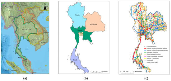
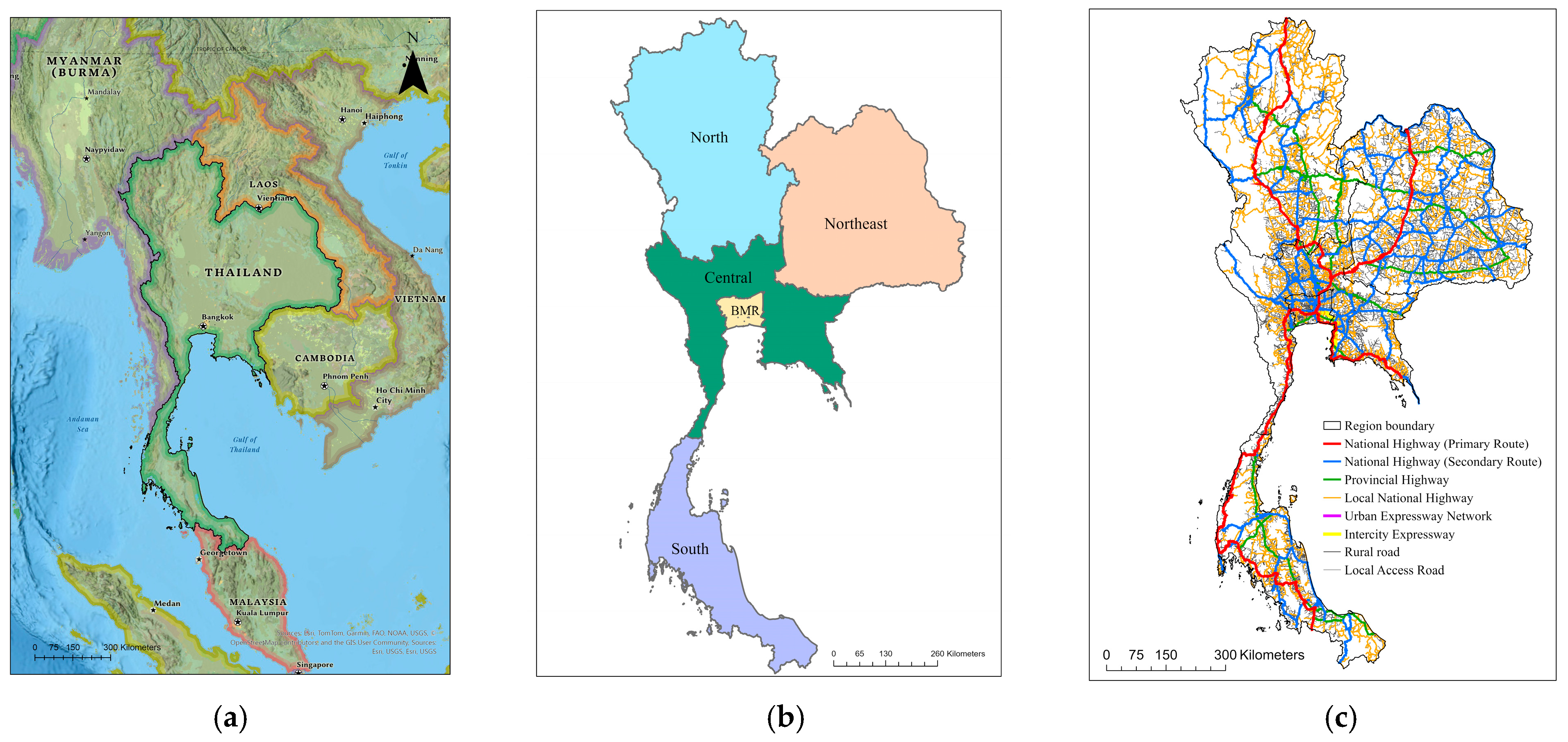
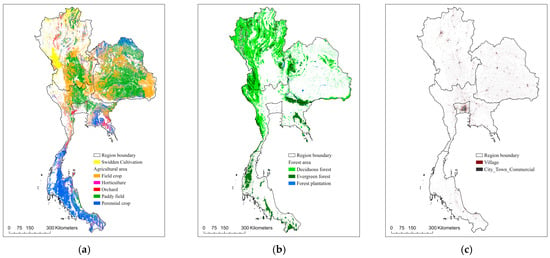
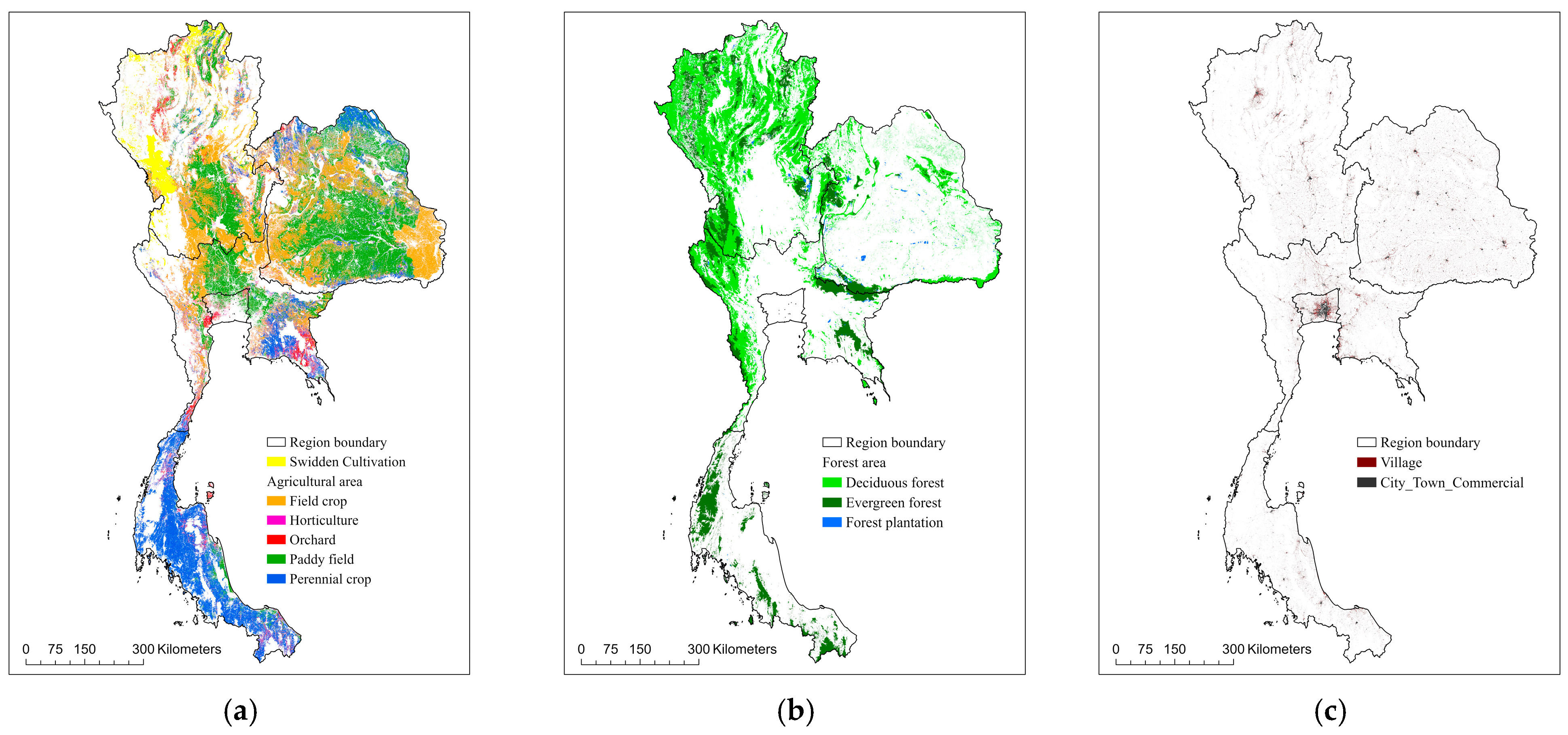
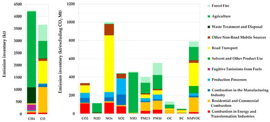
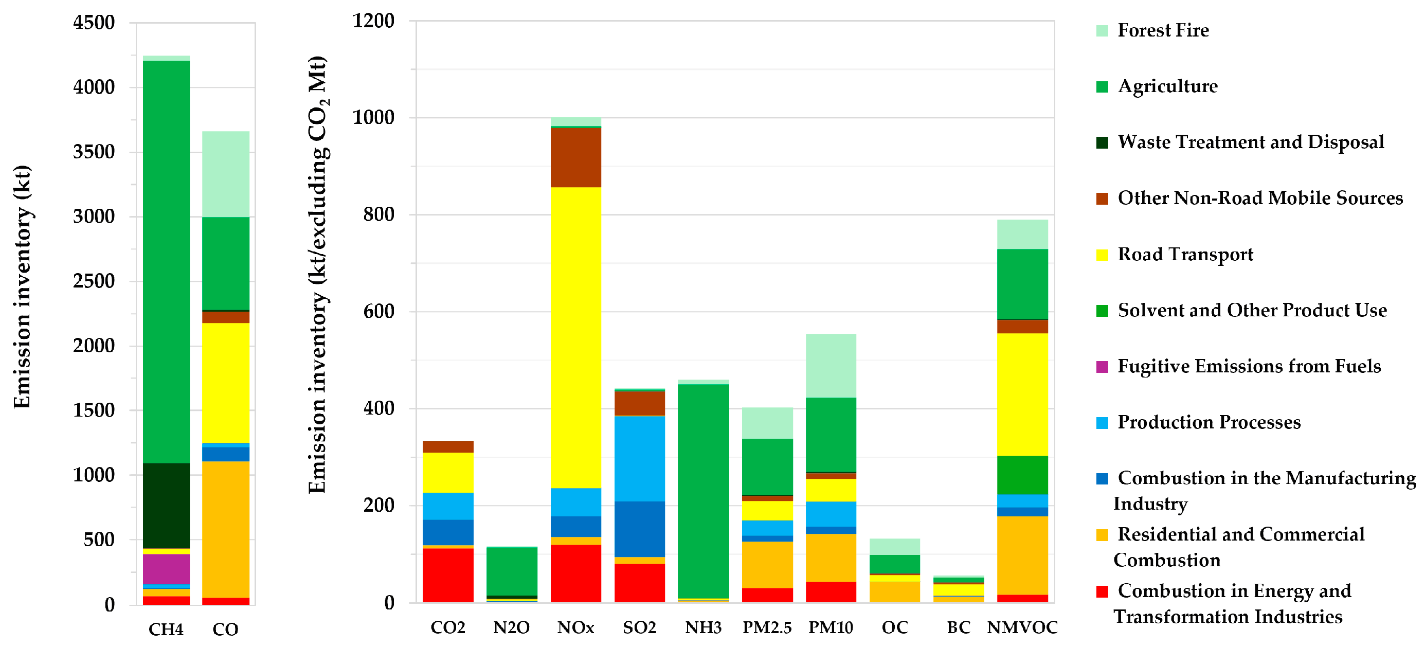
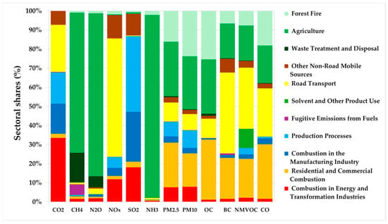
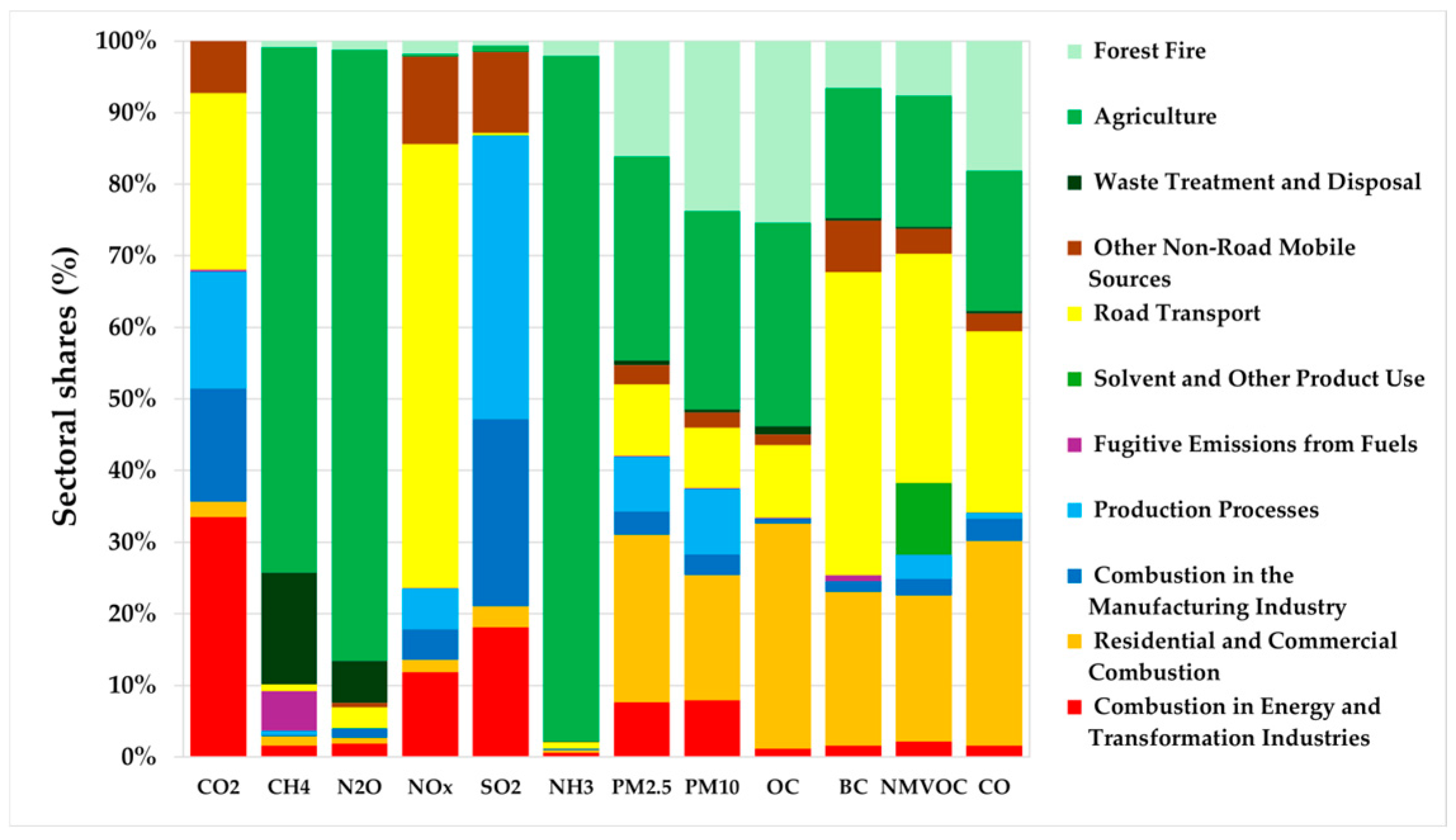
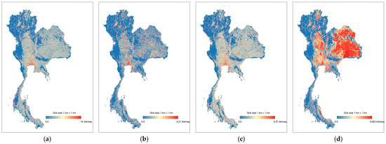
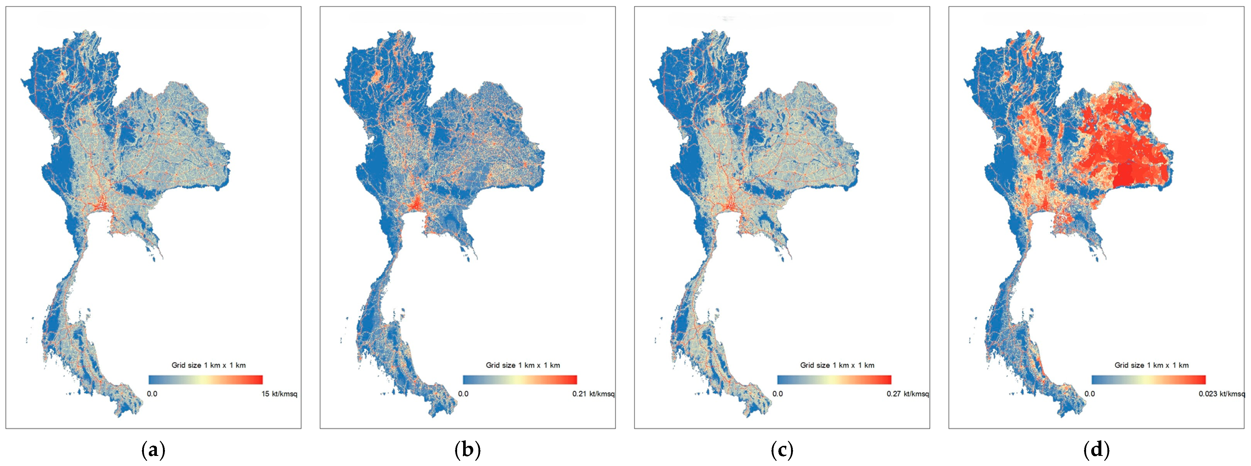
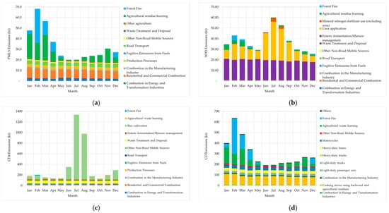
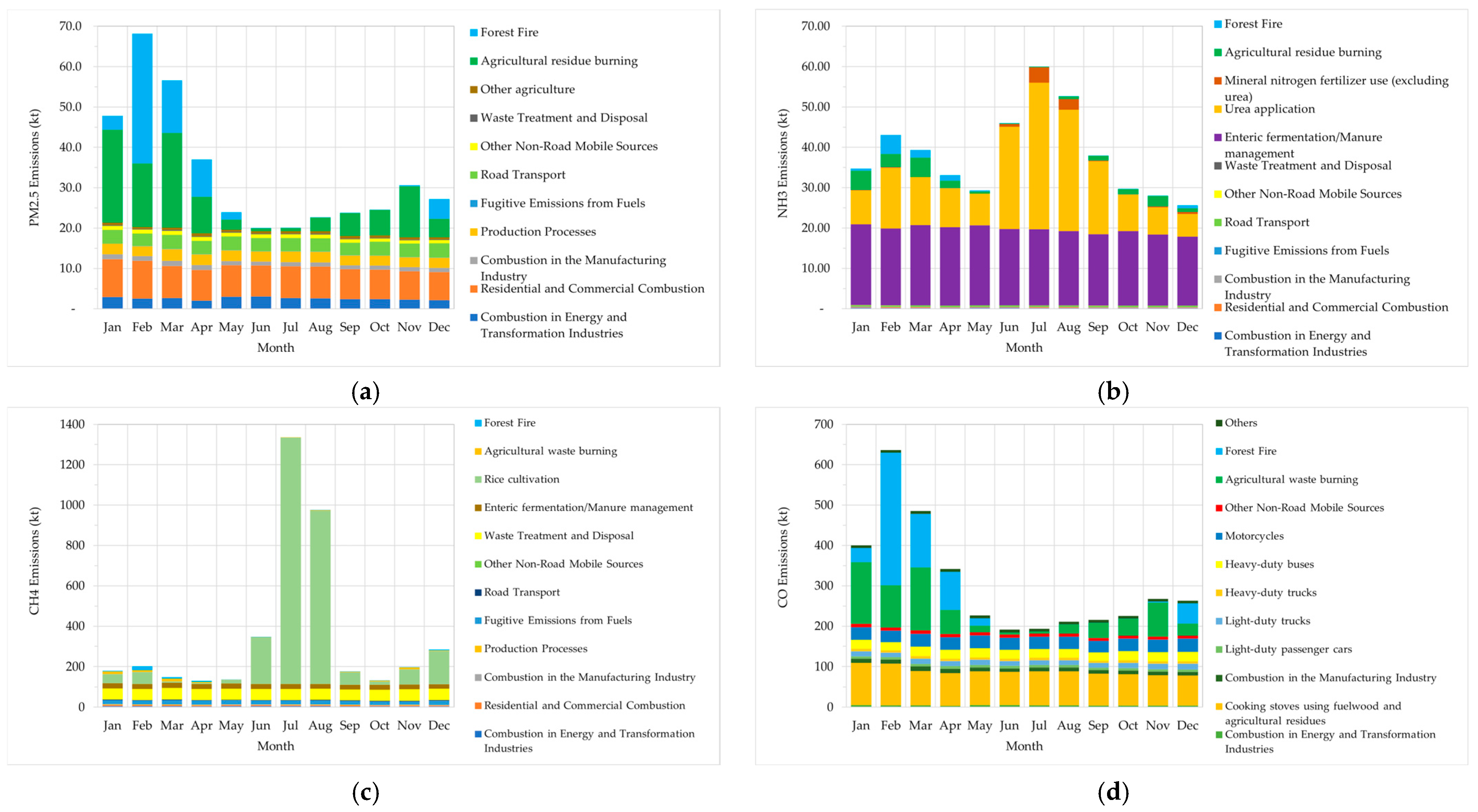
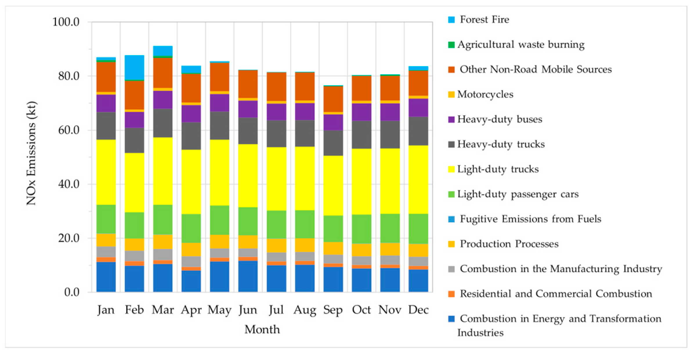
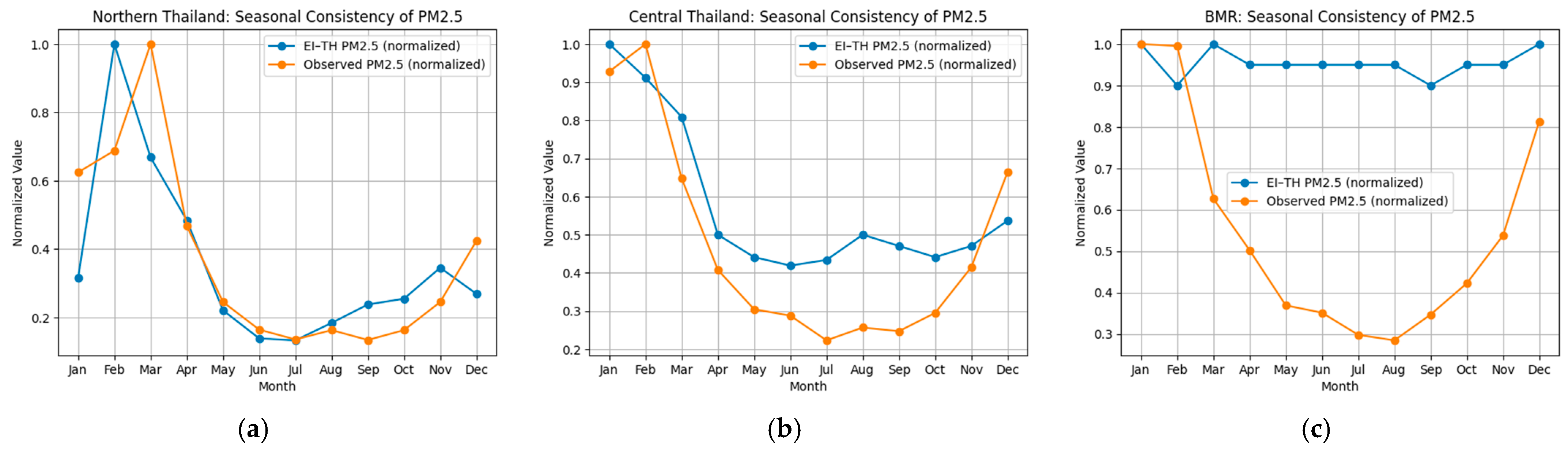
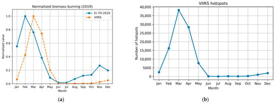
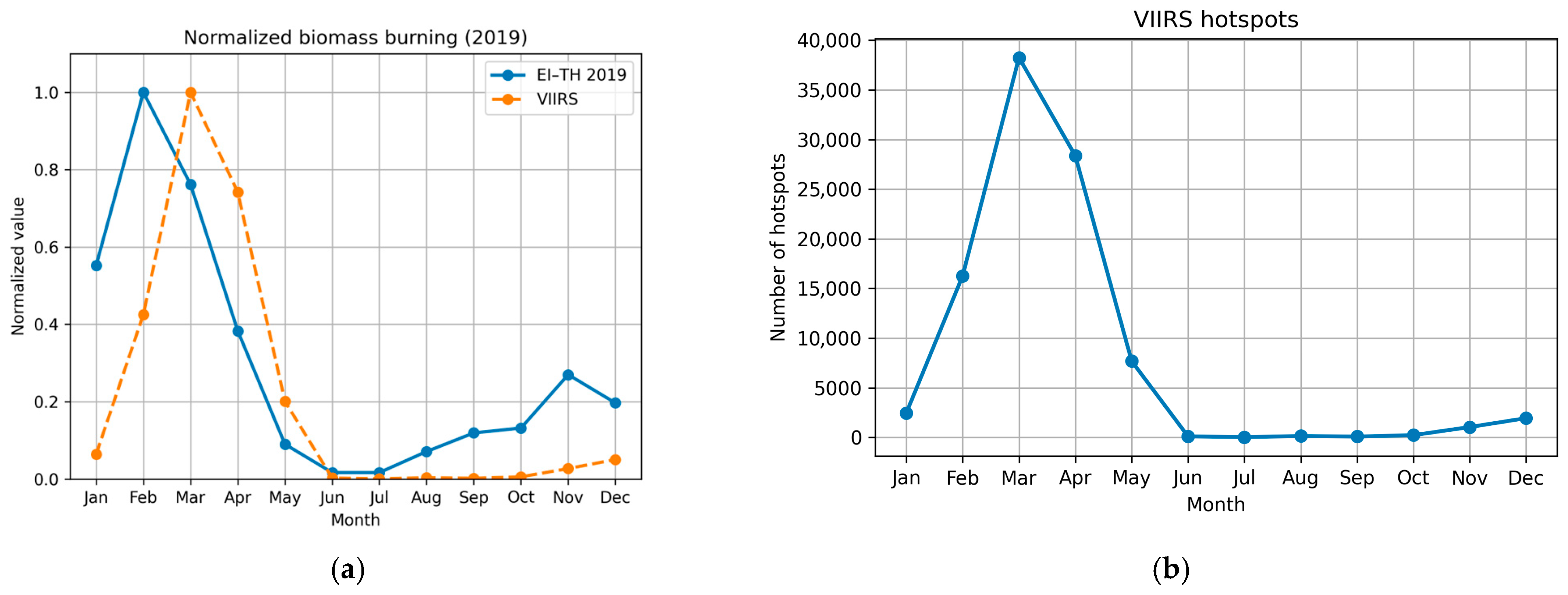
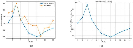
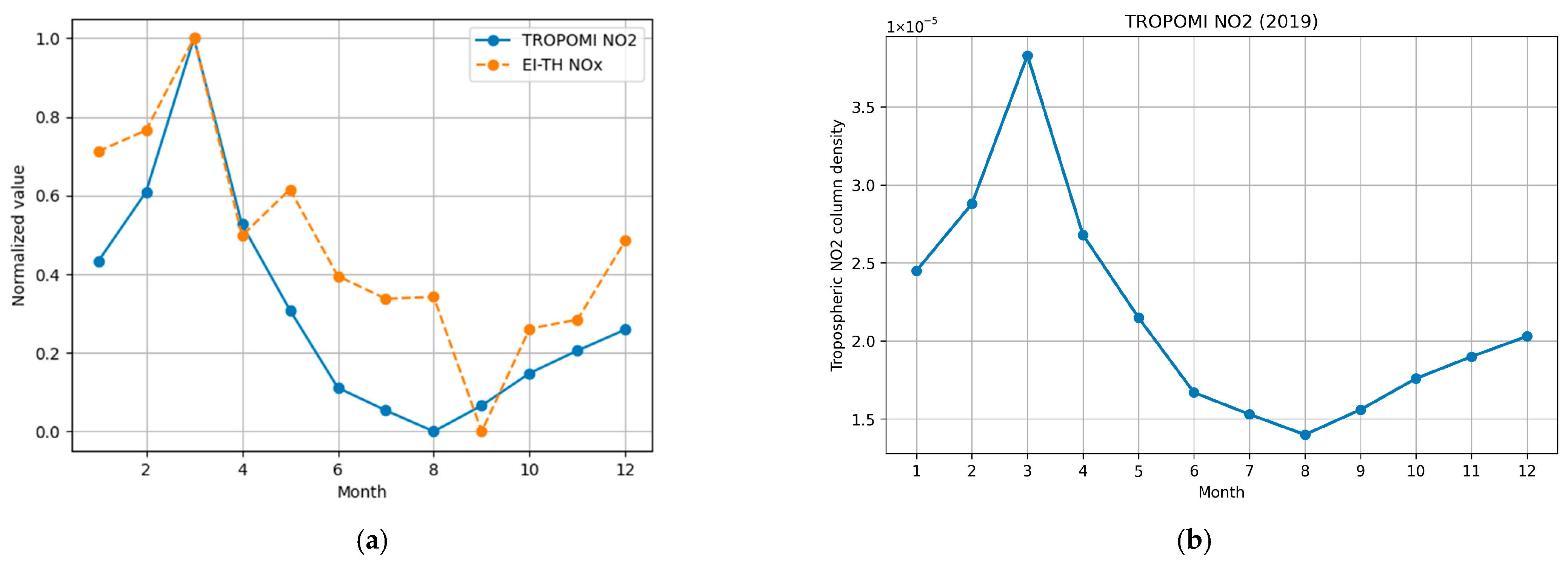
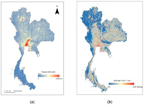
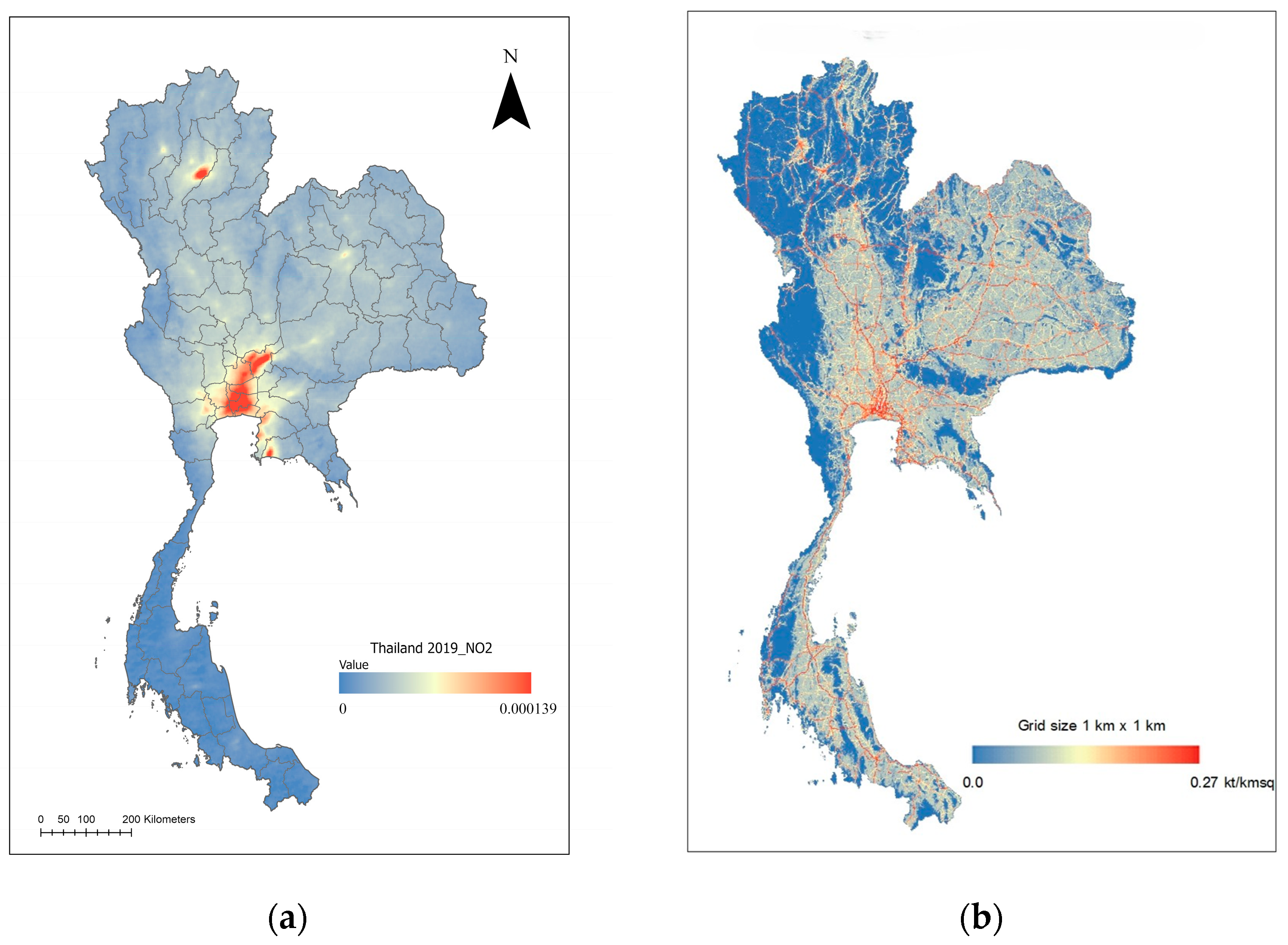
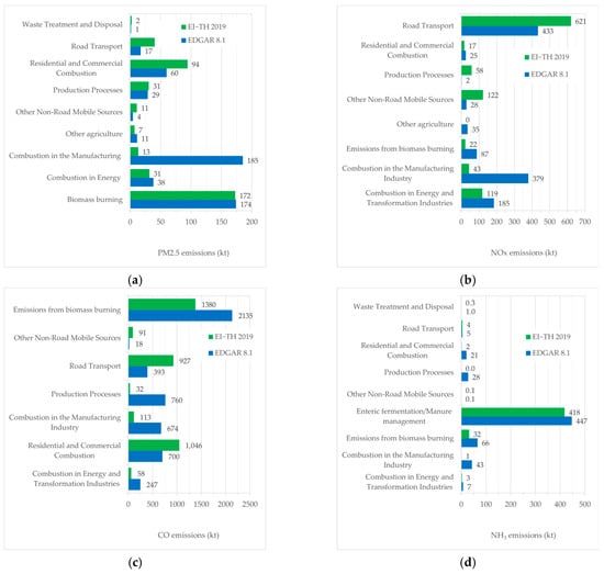
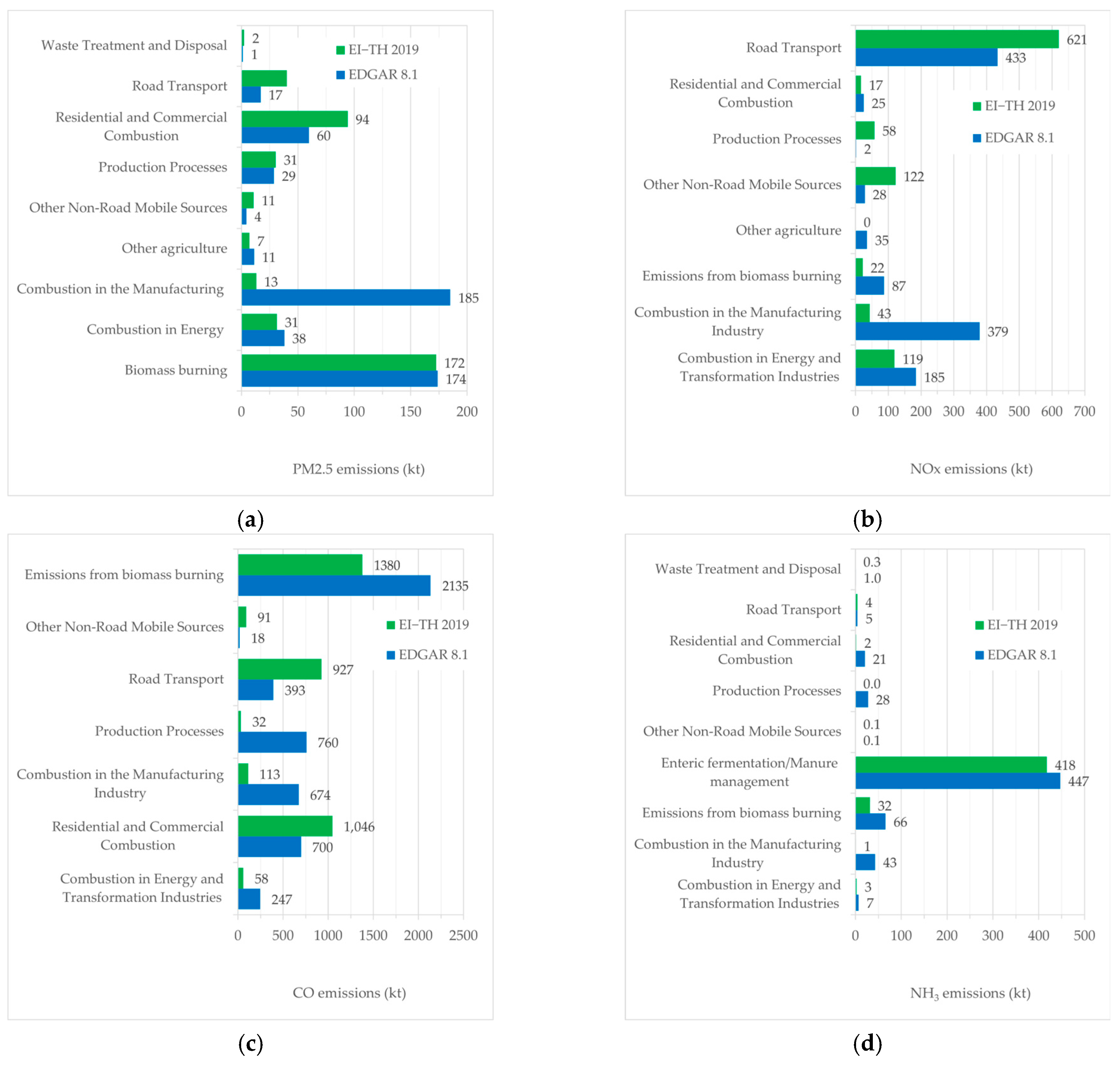
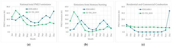
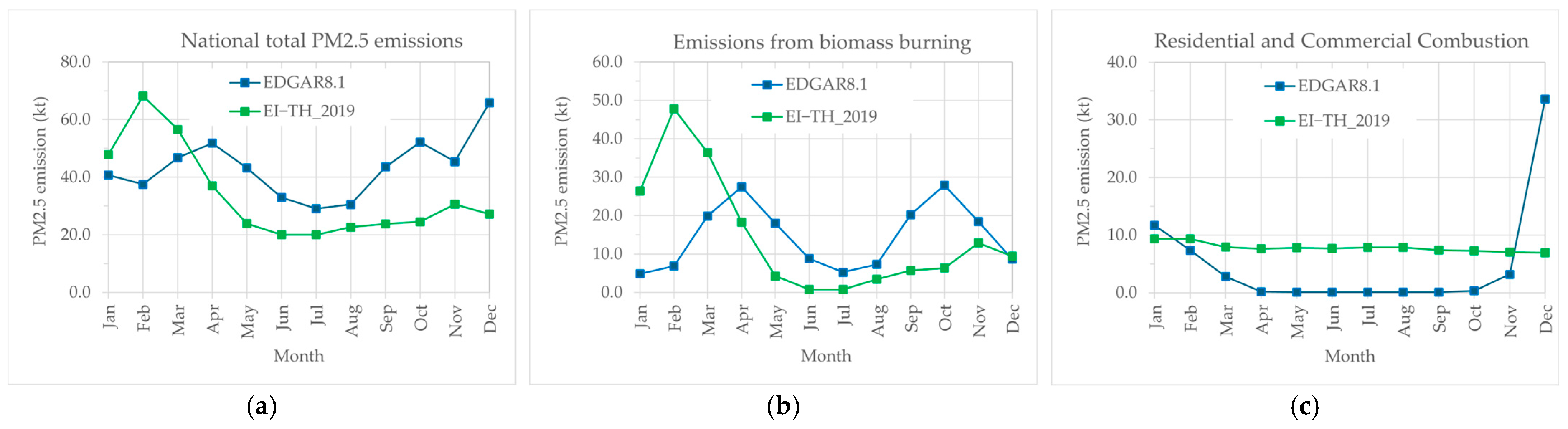
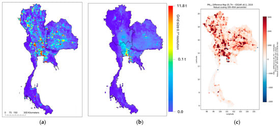
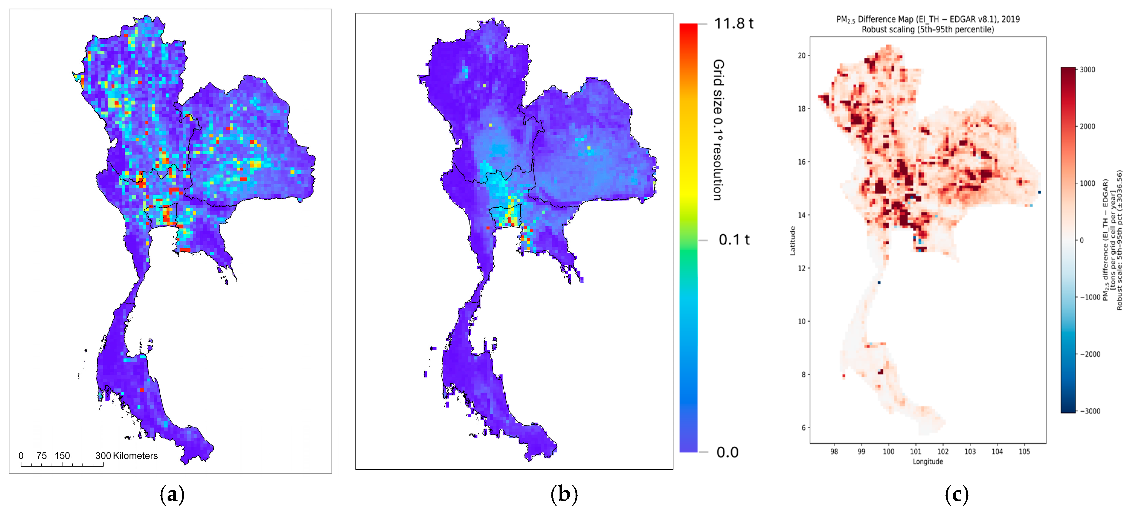
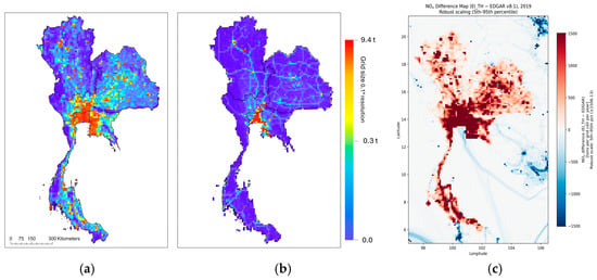
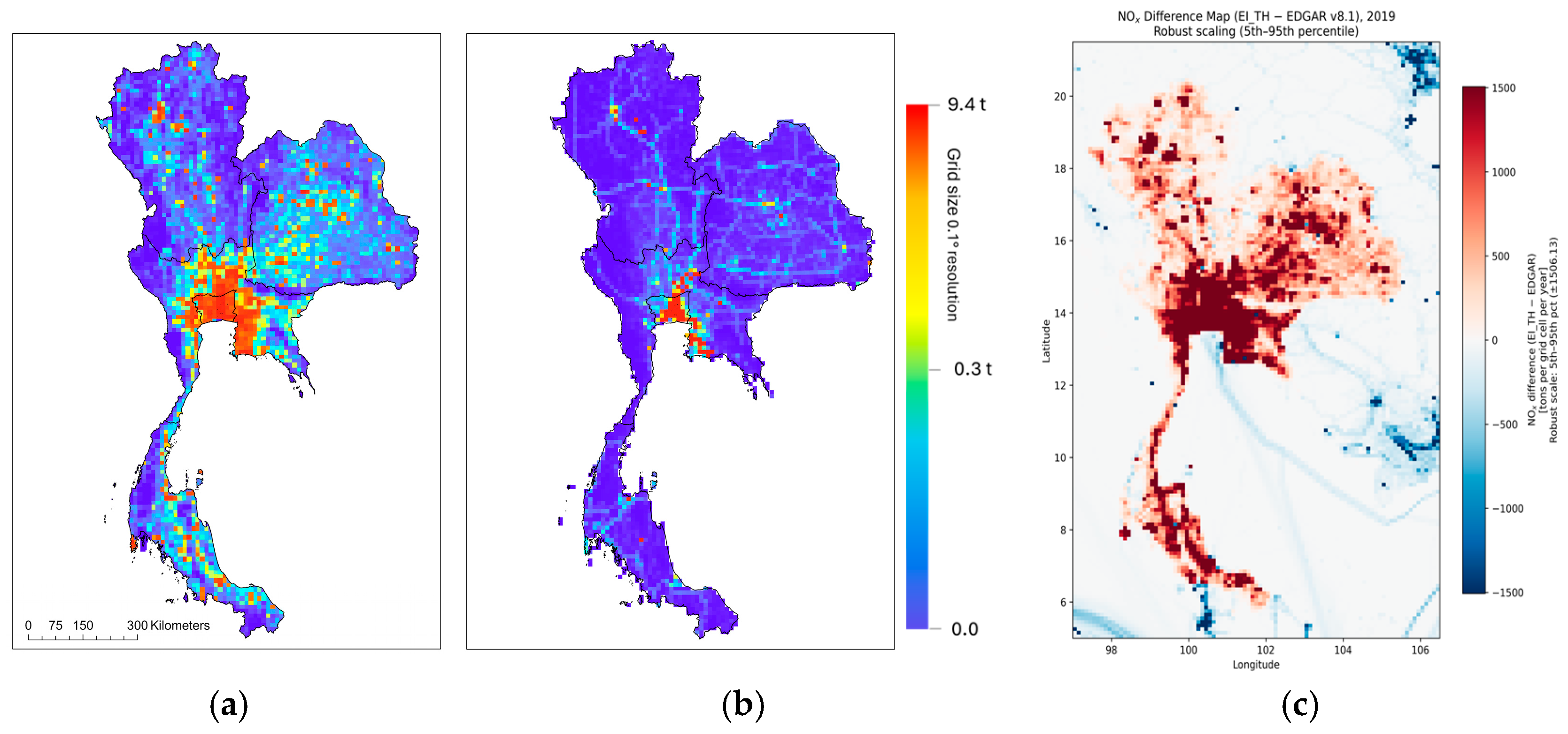
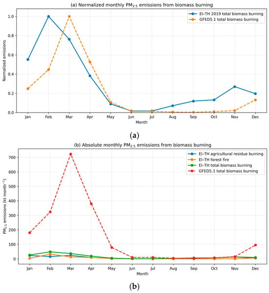
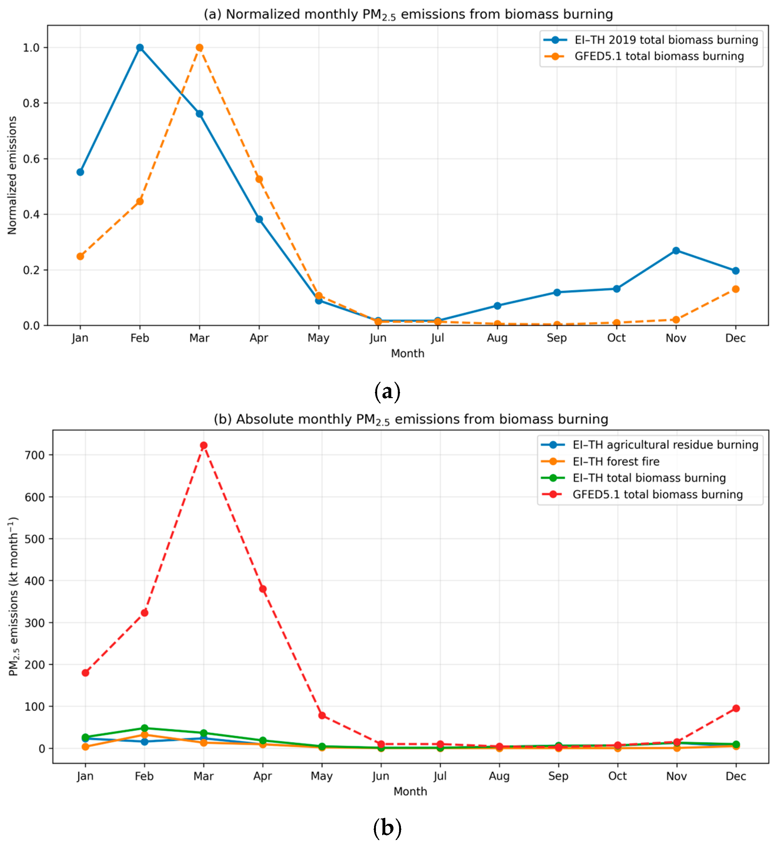

Disclaimer/Publisher’s Note: The statements, opinions and data contained in all publications are solely those of the individual author(s) and contributor(s) and not of MDPI and/or the editor(s). MDPI and/or the editor(s) disclaim responsibility for any injury to people or property resulting from any ideas, methods, instructions or products referred to in the content. |
© 2026 by the authors. Licensee MDPI, Basel, Switzerland. This article is an open access article distributed under the terms and conditions of the Creative Commons Attribution (CC BY) license.