Cross-Period Inference of Cropland Soil Organic Carbon Based on Its Relationship Patterns with Environmental Factors Incorporating the Seasonal Crop Rotation System

Abstract

Soil organic carbon (SOC) is a key indicator reflecting soil quality and management level. Understanding its spatiotemporal dynamics in cropland is necessary for sustainable land management. Revealing the relationship patterns between SOC (Sampling resolution: 1 km²; analysis resolution: 4 km²) and environmental factors in one period allows inferring SOC distribution in unsampled years, partly compensating for temporal data gaps. This study introduces a season-based crop rotation system (Winter wheat in the first season and summer corn in the next) as independent variables in a machine learning model innovatively, enriching variable selection in SOC inference and improving understanding of SOC accumulation. The Beijing–Tianjin–Hebei (BTH) region, characterized by a typical winter wheat–summer corn rotation system, was selected for analysis. The results show that in 2000, the average SOC was relatively low compared with global levels. Climatic variables were negatively correlated with SOC below the 0.8 quantile but positive above it, which corresponds to the upper 20% of the observed range of each climatic variable. Winter-wheat growth is more important on SOC distribution than summer-corn growth (two annual peaks of NDVI and EVI), showing a positive correlation with SOC, while corn showed a weak correlation and became negative above the 0.8 quantile. In the inferred results, the differences between observed and inferred mean values and their confidence intervals were approximately 0.1. This research provides a reference method for evaluating regional-scale SOC distribution patterns under data-limited conditions by integrating environmental factors and crop rotation characteristics.

1. Introduction

Soil organic carbon (SOC) is an important component of the global carbon pool, with a global storage of about 1500 Pg, playing a crucial role in the global carbon cycle [1,2]. In soils, SOC serves as a key nutrient that reflects soil fertility, functions as an indicator of soil quality, and partly represents the level of soil management [3,4]. However, the collection of SOC field samples is time-consuming and labor-intensive, especially in regions with large spatial extents, making it impossible to obtain SOC data for every time period needed. Therefore, to accurately evaluate soil management performance, it is necessary to estimate SOC distribution during periods without field sampling. By extracting the spatial relationship patterns between SOC and environmental factors from field-sampled data in one period, and then inferring SOC distribution for unsampled periods, this approach provides a practical solution that has been supported by previous studies [5,6,7].

Machine learning has been widely applied to identify relationship patterns between SOC and environmental factors. Commonly used methods include Random Forest and XGBoost [8,9]. Random Forest, a type of “boosting tree model”, has been proven reliable through extensive applications [10]. XGBoost, an implementation of the Gradient Boosting Decision Tree (GBDT), further improves predictive performance through optimized boosting algorithms [11]. LightGBM represents a subsequent optimization of XGBoost, offering higher computational efficiency and better prevention of overfitting while maintaining comparable accuracy [12]. Although LightGBM has been less frequently applied in SOC-related research, its potential advantages make it worth exploring. In addition, machine learning can capture the nonlinear effects of predictor variables on the target variable, thereby providing a more realistic interpretation of the mechanisms influencing SOC.

When exploring the relationship patterns between SOC and environmental factors and making further temporal inferences, different studies have selected various input variables. Adeniyi et al. incorporated soil, terrain, and vegetation factors to analyze the relationship between SOC and environmental conditions near river areas. Using land use and land cover (LULC) data as vegetation indicators, they found that the distance of sampling sites from the river was the most influential factor affecting SOC [13]. Wang et al. employed human, climatic, and land use factors [14] to explore their relationships with SOC in croplands and found temperature to be the dominant factor. However, these studies did not consider vegetation differences within crop rotation systems based on season. It is well known that rotation systems involve different crops across seasons, and these crops may have distinct relationships with SOC. Some researchers, such as Qu et al., considered the effects of rotation systems and analyzed soil properties, climatic factors, spatial distance, and rotation effects, but their classification of rotation systems was spatial rather than seasonal [15]. Other studies extended this line of research to infer SOC dynamics. Yang et al. used vegetation and climatic factors to develop an approach for predicting SOC distribution in unsampled years and verified its applicability across China [5]. The results showed that the spatial correlations between SOC and environmental factors were consistent with their temporal variations, confirming the feasibility of this method. Zhang et al. applied a similar approach using vegetation and climatic factors in the Dafeng Nature Reserve [6], demonstrating its validity on a smaller spatial scale. Song et al. further incorporated vegetation and land use factors to project SOC changes up to 2080, suggesting that this method can provide valuable insights for future SOC management [7].

A comprehensive review of previous studies reveals that there are certain differences in the selection of environmental factors between studies focusing only on the relationship patterns between environmental factors and SOC and those aiming to infer SOC distribution. Studies that examine relationship patterns typically include variables requiring field sampling to represent current conditions (e.g., soil properties and human activities), as well as remotely sensed open-access data (e.g., vegetation and climatic factors). In contrast, studies inferring SOC distribution for unsampled years can only rely on multi-temporal variables derived from open-access remote sensing data. These studies did not classify vegetation factors according to the seasons of the crop rotation system. Therefore, how different types of vegetation based on season-of-rotation systems influence SOC at a large spatial scale remains unclear.

This study is based on multi-period open-access remote sensing data (e.g., vegetation and climatic factors) and single-period data with no significant temporal variation (e.g., terrain). The relationship patterns between SOC and environmental factors were established using field-sampled SOC data from one period in croplands of the Beijing-Tianjin-Hebei (BTH) region. These patterns were then applied to other unsampled periods to infer the potential SOC distribution. By innovatively introducing a rotation system classified by planting seasons and using vegetation parameters at the peak growth stages of two main seasons as input variables (the growth situation of winter wheat and summer corn), this study provides new insights into the relationship between environmental factors and SOC, and further explores how crop rotations influence SOC at a large spatial scale, and we hypothesize that different seasonal crops exert distinct effects on soil organic carbon dynamics.

2. Data and Methods

2.1. Research Area and Workflow

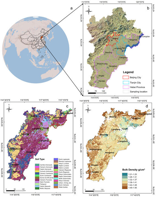
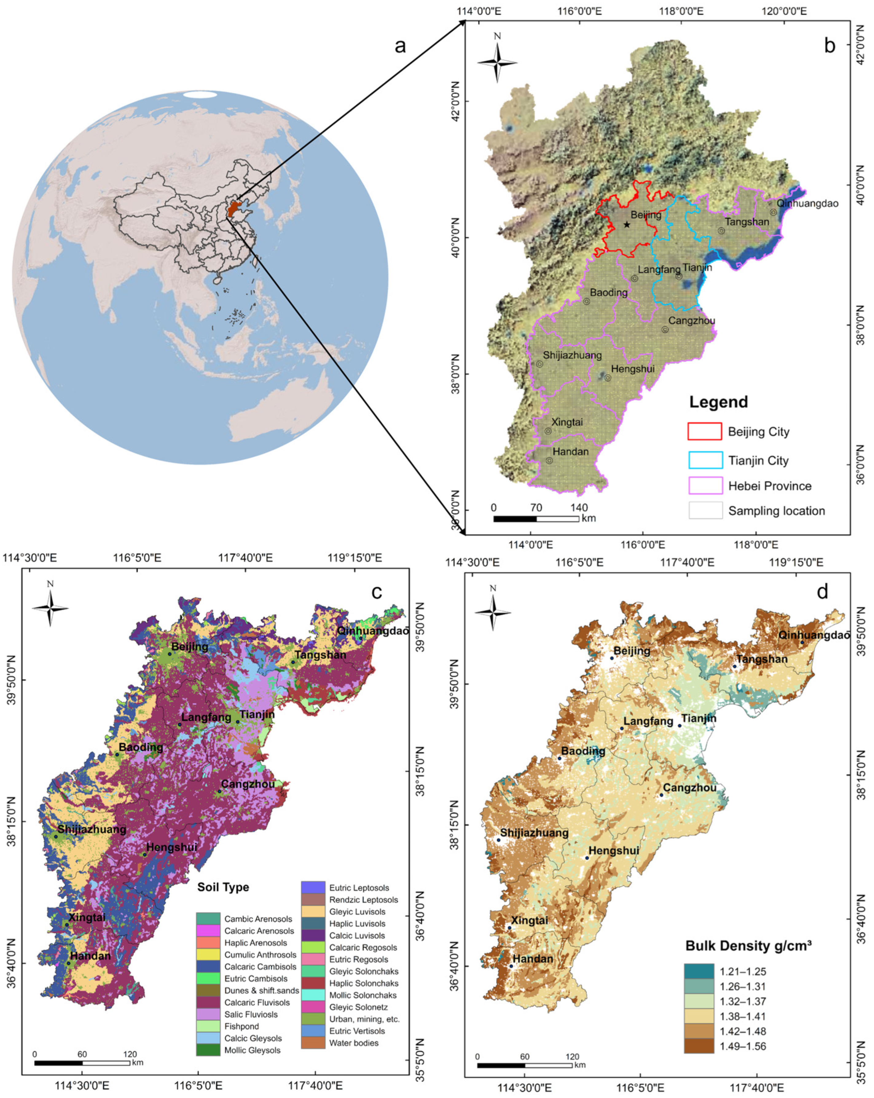
The research area is located on the southeastern plain of the BTH region, extending from 36°05′ to 42°40′ N and from 113°27′ to 119°50′ E. The basic geographic information of the research area, including location, administrative divisions, topography, soil types, and soil bulk density, is shown in Figure 1. The BTH region is an important economic, agricultural, and political center of China. In 2022, the region’s GDP reached 10.03 trillion yuan, with a permanent population of approximately 109.67 million. It forms the core area of northern China, characterized by abundant energy resources and a well-developed industrial base [16]. The climate in the region is mild with distinct seasonal variations. Between 2000 and 2020, annual precipitation ranged from 300 mm to 750 mm, and the mean annual temperature varied between 10.5 °C and 14.5 °C [17]. Cropping in this region typically follows a stable winter wheat–summer maize rotation system with large-scale cultivation. Therefore, the BTH region was selected as the research area to investigate the relationship patterns of crop rotation and other environmental factors on SOC.

Figure 1. The basic information of the research area: (a) location, (b) terrain and administrative divisions, (c) soil type, and (d) bulk density.

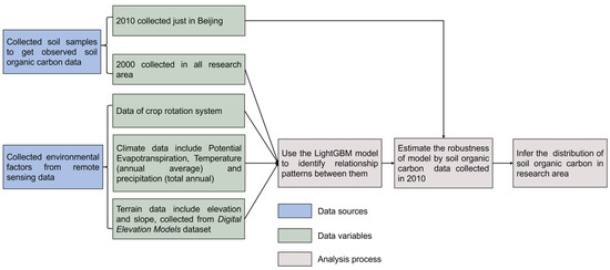
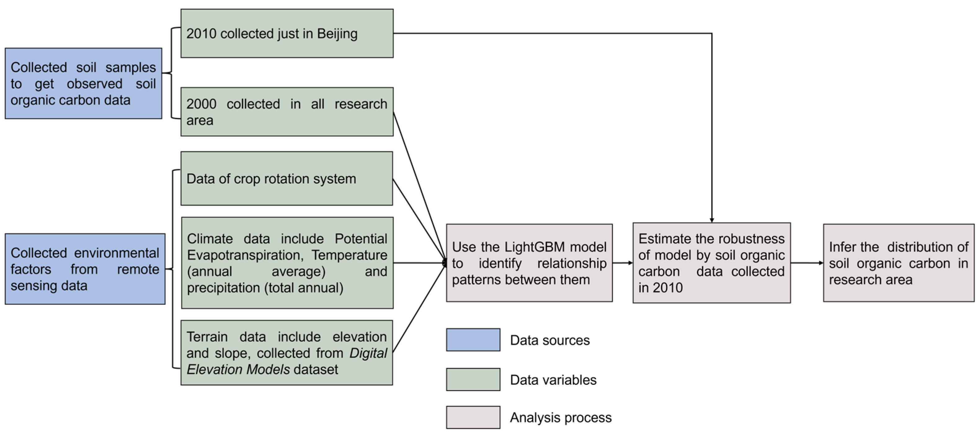
SOC data for 2000 and 2010 were obtained through field sampling and laboratory analysis, while environmental factors data were derived from publicly available datasets. The LightGBM model was used to identify relationship patterns between SOC and environmental factors based on the data in 2000, thereby establishing an inference model for SOC inference. The 2010 field-sampled SOC data from Beijing were then used to validate the model’s inference performance. Using this model, we inferred the spatial distribution of SOC for the years 2000, 2005, 2010, 2015, and 2020. The overall workflow is illustrated in Figure 2.

Figure 2. Workflow.

2.2. Research Data

The data used in this study consist of two components: SOC data and environmental data.

2.2.1. Soil Organic Carbon

The SOC data consists of two time periods. The first dataset, from the year 2000, covers the entire research area with a total sampled area of 100,904.57 km². These data were provided by the Institutes of Geological Survey in Tianjin, Hebei, and Beijing. The second dataset, from 2010, covers the plain area of Beijing, with a sampled area of 6613 km², and was obtained from the Beijing Institute of Geological and Mineral Exploration, Beijing Institute of Ecological Geology.

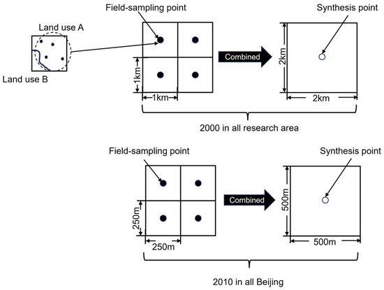
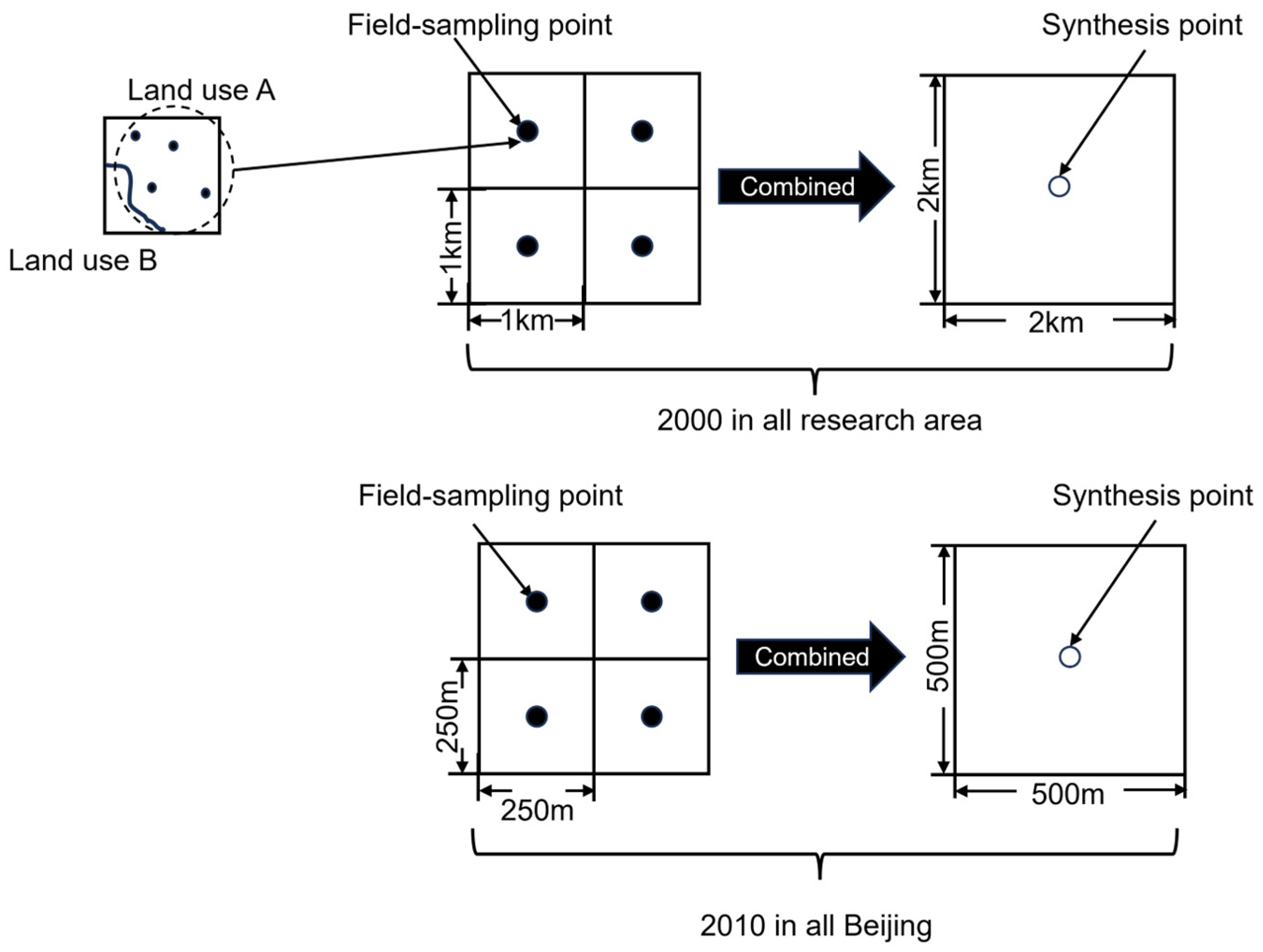
All sampling sites in this study were collected using the multi-purpose regional geochemical survey methods [18,19,20]. In 2000, SOC sampling was conducted at a scale of 1:250,000; in total, 75,684 samples were collected. Sampling locations were selected away from roads, industrial and mining enterprises, residential areas, and sites with evident pollution. All samples come from cropland. The coordinates of each sampling point were determined using GPS. Within a 100 m radius of each point, 3 to 5 subsamples were collected and thoroughly mixed in equal proportions to form a composite sample. Soil was collected from a depth of 0–20 cm, with each composite sample weighing approximately 2 kg. Samples were placed in clean cloth bags, air-dried, and then sieved through a 10-mesh nylon screen. The processed soil was subsequently stored in plastic sampling bottles. After the combination, 18,921 SOC data points were obtained. It should be noted that the four collected soil samples were physically mixed prior to analysis. This procedure does not involve post hoc numerical weighting or statistical compression of 75,684 independent SOC measurements.

In 2010, SOC sampling was conducted at a scale of 1:50,000; similarly, only the samples associated with cropland were used. Therefore, 29,884 cropland points were actually sampled, and 7471 remained after combination. The procedure of actual sampling and data combination for 2000 and 2010 is shown in Figure 3.

Figure 3. The sampling method of the multi-purpose geochemical survey.

The methods for sample collection and processing in 2010 were the same as those used in 2000. However, due to the higher testing density of the 2010 soil samples, the measured data used the resampled method in ArcGIS 10.2 to a density of one point per 4 km² to allow for a consistent comparison between the inferred results and the observed data.

The SOC content was determined via the volumetric oxidation-reduction method (VOL) by reacting 0.5 g of the sieved samples with K₂Cr₂O₇–H₂SO₄ solution in a heated sand bath. The total carbon content was measured by infrared spectroscopy by broiling 0.1 g of the sample in a high-frequency furnace [21]. To ensure analytical precision and accuracy, four standard reference samples were included in each analytical batch (consisting of 50 samples) and analyzed alongside the soil samples. Accuracy was assessed by calculating the deviation between the measured and certified values of the standard samples using the formula $\Delta lgC=\left|lgC\right(observed)-lgC(standard\left)\right|$. Precision was evaluated using the formula $\lambda =\sqrt{{\displaystyle \frac{{\sum }_{i=1}^n(\mathit{lg}{C}_{observed}-\mathit{lg}{C}_{standard}{)}^2}{4-1}}}$ where $n$ = 4. The analytical results were considered valid if $\Delta lgC$≤ 0.07 and $\lambda$ ≤ 0.10, with an acceptable pass rate of no less than 98%. In the experiments, SOC content was expressed as “Corg/%”. Therefore, the figures in this paper also use “Corg/%” to represent SOC content.

2.2.2. Environmental Factors

The environmental factors used in this study include vegetation, climate, and terrain, all of which were obtained from publicly available datasets, as summarized in Table 1.

Table 1. Data on environmental factors.

Data Type	Data Name	Spatial Resolution	Time Resolution	Unit (Original Data)	Reference
Soil	LU	30 m2	Year	-	[22]
	BD	-	-	g/cm3	[23]
	Soil type	-	-	-
Vegetation	NDVI	250 m2	16 day	-	[24]
	EVI	250 m2	16 day	-
Climate	PRE	1 Km2	Month	0.1 mm	[25]
	TMP	1 Km2	Month	0.1 °C	[26]
	PET	1 Km2	Month	0.1 mm	[27]
Terrain	EL	30 m2	-	m	[28]
	SL	30 m2	-	°

Note: the abbreviations of data are as follows: Land use (LU), Bulk density (BD), Normalized Difference Vegetation Index (NDVI), Enhanced Vegetation Index (EVI), precipitation (PRE), Temperature (TMP), Potential Evapotranspiration (PET), Elevation (EL), Slope (SL).

When extracting environmental factors, spatial consistency between environmental variables and SOC data must be ensured. In this study, the SOC observation unit represents a composite sampling unit of approximately 4 km². Therefore, environmental variables were resampled from their original spatial resolution (e.g., 30 m) to 4 km² to match the SOC analysis scale. Although this transformation may smooth local spatial heterogeneity to some extent, the SOC data themselves already represent the average condition within the 4 km² sampling unit. Environmental datasets were first resampled to the SOC analysis scale using the Resampling tool in ArcGIS. The “Extract Multi Values to Points” tool was then used to extract the resampled environmental variables to the SOC sampling locations, establishing a one-to-one correspondence for subsequent modeling analysis.

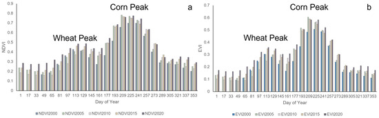
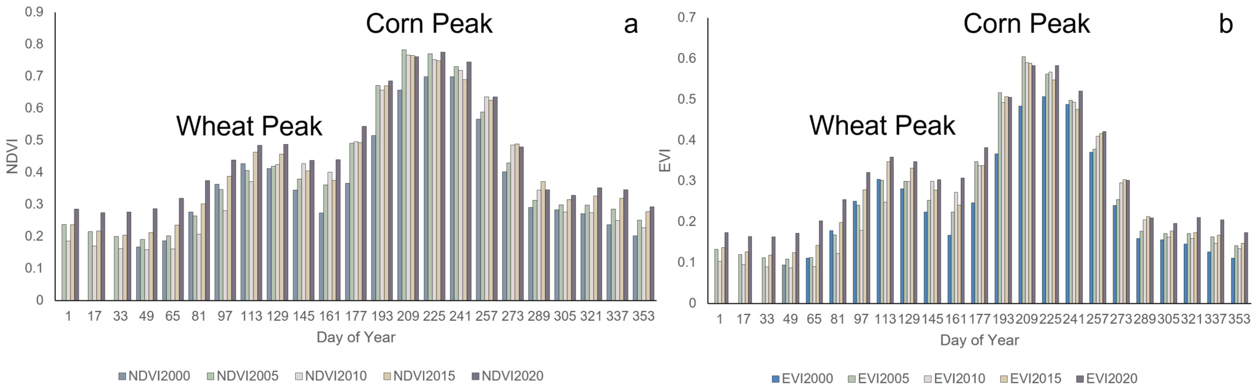
The rotation system divided by season is an important variable in this study. Due to the wheat–corn rotation system in this region, vegetation-related indices typically exhibit two distinct annual peaks. These peaks correspond to the growth and residue production of wheat and corn, respectively, and can serve as indicators of seasonal organic carbon inputs to the soil. We refer to these as the “wheat peak” and the “corn peak.” The identification of these two peaks is illustrated in Figure 4.

Figure 4. The ‘wheat peak’ and the ‘corn peak’ during the research year. (a) NDVI; (b) EVI.

As shown in the figure, although the timing of the wheat and corn peaks in NDVI and EVI differs slightly, the overall difference is minimal. These results indicate that winter wheat is generally harvested between April and May, and summer corn between August and September. The NDVI and EVI values on the identified peak dates were selected as vegetation variables and, together with climatic and topographic variables, were used as environmental factors for model training.

The climate factors include temperature (TMP), annual precipitation (PRE), and potential evapotranspiration (PET). TMP and PET represent the annual average values, while PRE refers to the total annual precipitation. PET refers to the water from moist soil that evaporates into the air and can indicate the soil’s water-holding capacity. The terrain factors include elevation (EL) and slope (SL). Since terrain remains relatively stable over short time periods, a single-period dataset was used to represent the overall terrain conditions.

2.3. Research Method

LightGBM was chosen to find relationship patterns between environmental factors and SOC to make an inference model because it performs well with large and complex datasets and, compared with traditional models, can better avoid overfitting, making it worth applying in soil-related studies. The model of lightGBM is shown in Equation (1) [12].

$${\tilde{V}}_j(d)={\displaystyle \frac{1}{n}}\left({\displaystyle \frac{({\sum }_{x_i\in A_l} g_i+\frac{1-a}{b}{\sum }_{x_i\in B_l} g_i{)}^2}{n_l^j(d)}}+{\displaystyle \frac{({\sum }_{x_i\in A_r} g_i+\frac{1-a}{b}{\sum }_{x_i\in B_r} g_i{)}^2}{n_r^j(d)}}\right)$$

(1)

In the equation, $V_j\left(d\right)$ denotes the variance gain of feature $j$ at split point $d$. $O$ represents the training dataset at the current decision tree node. $g_i$ is the gradient of data point $i$, and $n_O$ is the number of data points in $O$. $n_{l|O}^j\left(d\right)$ and $n_{r|O}^j\left(d\right)$ indicate the number of data points assigned to the left and right child nodes, respectively, after the split based on feature $j$ at point $d$.

Compared with the traditional GBDT model, Equation (1) introduces two distinct subsets of the dataset: subset A, which contains data points with larger gradients, and subset B, which contains data points with smaller gradients. $A_l$ and $A_r$ represent the subsets of larger-gradient samples that are assigned to the left and right child nodes, respectively. $B_l$ and $B_r$ denote the subsets of smaller-gradient samples, which are randomly sampled and then assigned to the left and right child nodes, respectively. After sampling the smaller-gradient subset B, a weighting factor of ${\displaystyle \frac{1-a}{b}}$ is applied to compensate for the effect of resampling. As a result, using LightGBM to train the inference model significantly reduces the computational cost while maintaining a comparable level of inference accuracy. In this study, the dataset was randomly split into a training set (80%) and a test set (20%) for model inference using LightGBM. The LightGBM model was implemented using the lightgbm package in R (version 4.5.0; R version 4.0.5). Additionally, 10-fold cross-validation was performed to evaluate the model’s stability and generalization ability.

In this model, the dependent variable is the observed SOC in 2000, and the independent variables include climate, vegetation, and terrain. Although SOC is also affected by human activities and soil properties, these variables are difficult to obtain and cannot be used in high-resolution spatiotemporal SOC inference. In this study, climate and vegetation variables can be obtained annually from remote sensing datasets, while terrain factors remain largely unchanged over time; therefore, their temporal variations are not considered. To obtain the optimal parameters, we used a Bayesian process for optimization.

The accuracy of the inference model is evaluated using the coefficient of determination (R²) and the Root Mean Square Error (RMSE), as defined in Equations (2) and (3), respectively.

$${\mathrm{R}}^2={\displaystyle \frac{{\sum }_{\mathrm{i}=1}^{\mathrm{n}} {\left({\mathrm{X}}_{\mathrm{i}}-\overline{{\mathrm{Y}}_{\mathrm{i}}}\right)}^2}{{\sum }_{\mathrm{i}=1}^{\mathrm{n}} {\left({\mathrm{Y}}_{\mathrm{i}}-\overline{{\mathrm{Y}}_{\mathrm{i}}}\right)}^2}}$$

(2)

$$\mathrm{R}\mathrm{M}\mathrm{S}\mathrm{E}=\sqrt{{\displaystyle \frac{1}{n}}{\sum }_{i=1}^n {\left(X_i-Y_i\right)}^2}$$

(3)

In Equations (2) and (3), $X_i$ and $Y_i$ represent the observed and inferred values of SOC content, respectively, and $n$ denotes the number of samples.

When finding the relationship patterns, the indicators Gain and Cover from the LightGBM framework were used to evaluate the importance of different predictor variables. Specifically, Gain indicates the extent to which a factor improves model accuracy during inference, while Cover represents the number of samples involved when the feature is split. Together, they reflect the importance of the factor in shaping the spatial distribution of SOC [12].

Equation (4) was used to convert SOC content into soil organic carbon density (SOCD):

$$SOCD=Corg\left(\%\right)\times BD\times D\times 100$$

(4)

In Equation (4), SOCD represents soil organic carbon density, expressed in t/km². BD refers to the soil bulk density, with units of g/cm³. D denotes the sampling depth of the soil profile in centimeters; in this study, all samples were collected at a uniform depth of 20 cm.

3. Results

3.1. SOC Inference Model and Its Robustness

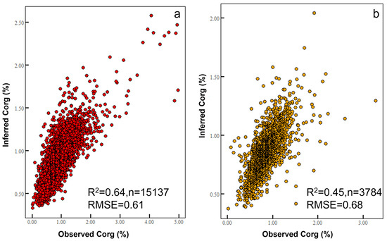
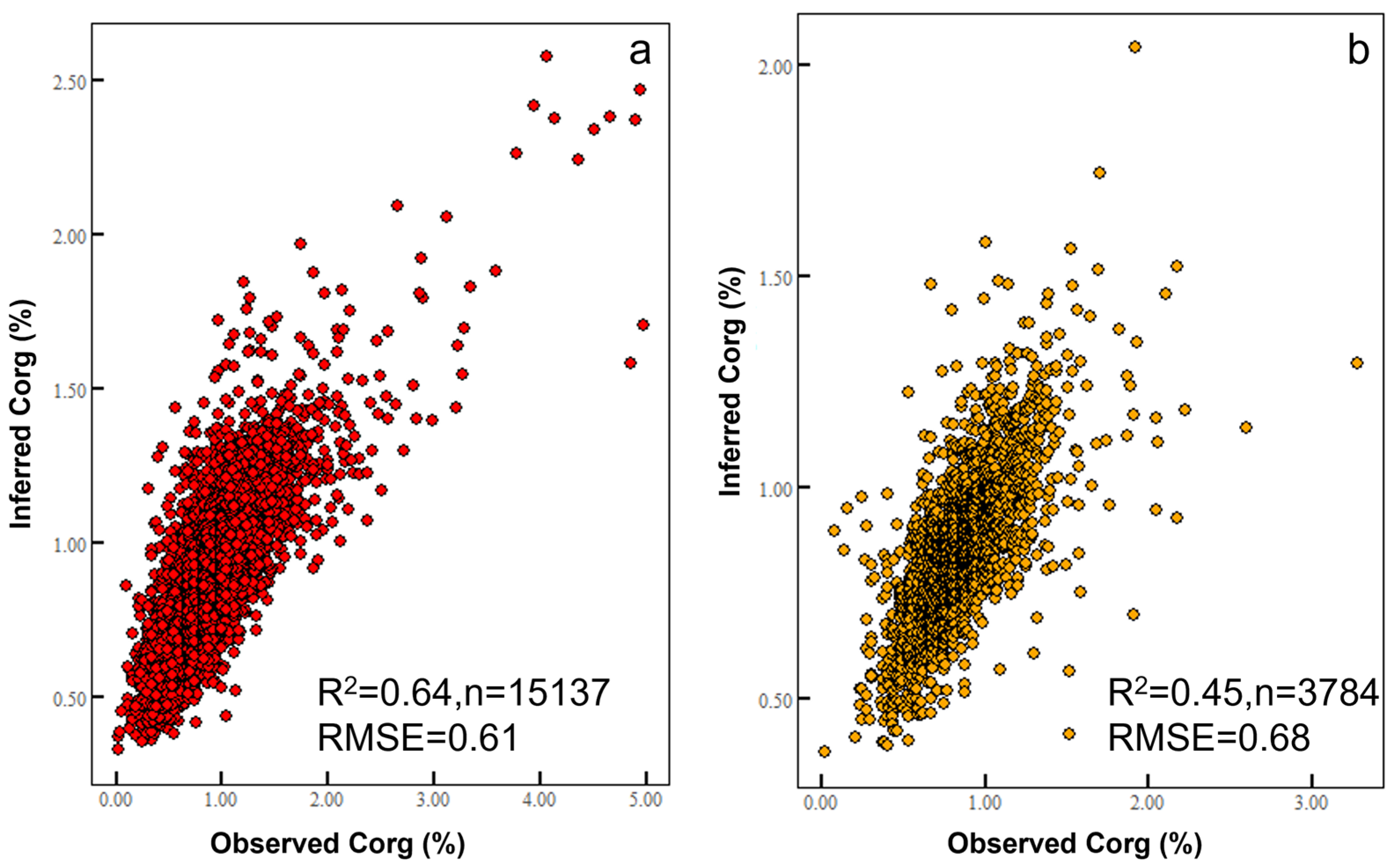
To infer SOC in unsampled years, we constructed the inference model and verified it. Figure 5 presents the model constructed according to the procedure described in Section 2.3. After training and testing, the R² values for the training and testing sets were 0.64 and 0.45, respectively, with corresponding RMSE values of 0.63 and 0.73. The training and testing sets contained 15,137 and 3784 samples, respectively.

Figure 5. Accuracy of the training and testing sets in the SOC inference model. (a) Training set, (b) Testing set. Note: This figure shows the observed SOC in 2000 and the values inferred by inference model using environmental factors. The dataset was randomly divided into training and testing sets at a ratio of 8:2, with the testing set not involved in training.

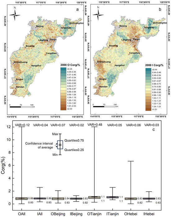
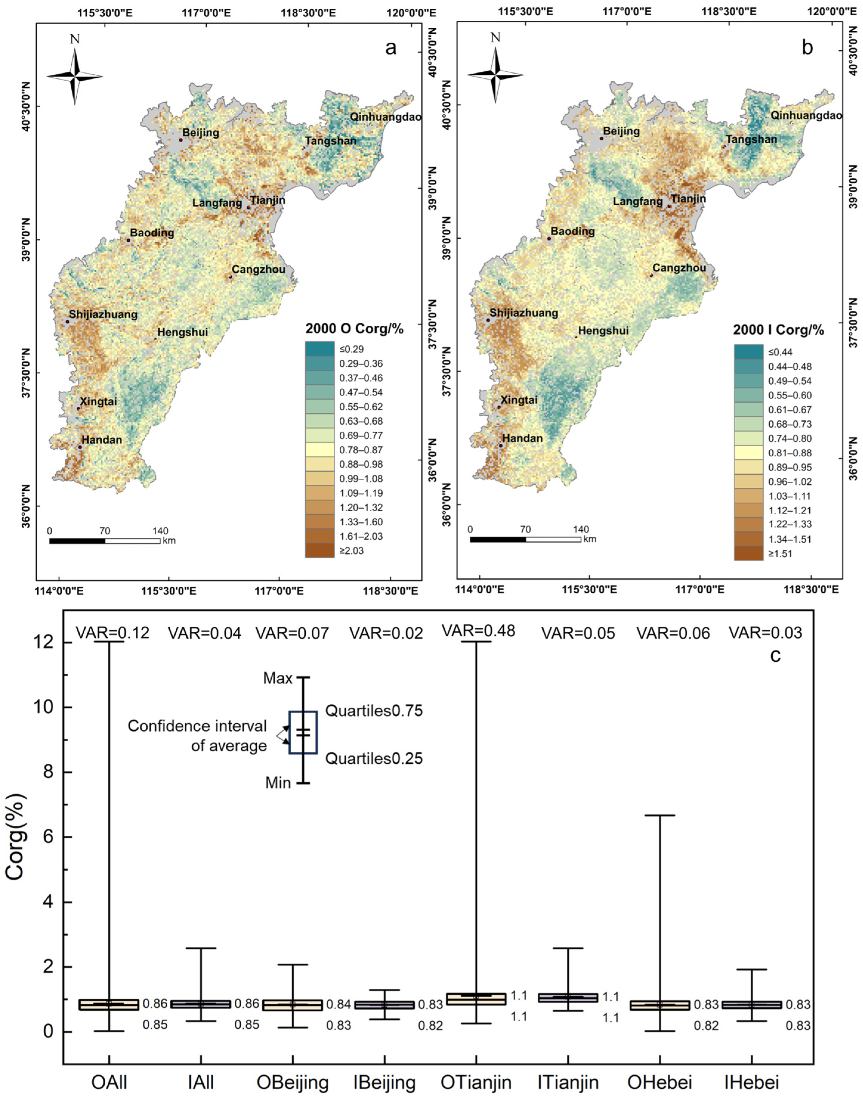
A comparison between the inference and observed spatial distributions of SOC content in the year 2000 shows a high degree of consistency, as illustrated in Figure 6. From a quantitative perspective, the average SOC content for both the inference and observed data is 0.85%.

Figure 6. Inferred and observed spatial distributions of SOC content. (a) Inferred, (b) Observed. (c) The variance and confidence interval of the observed and inferred values in each area. Note: O is the value that can be observed, I is the value that can be inferred.

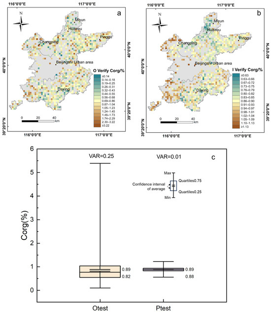
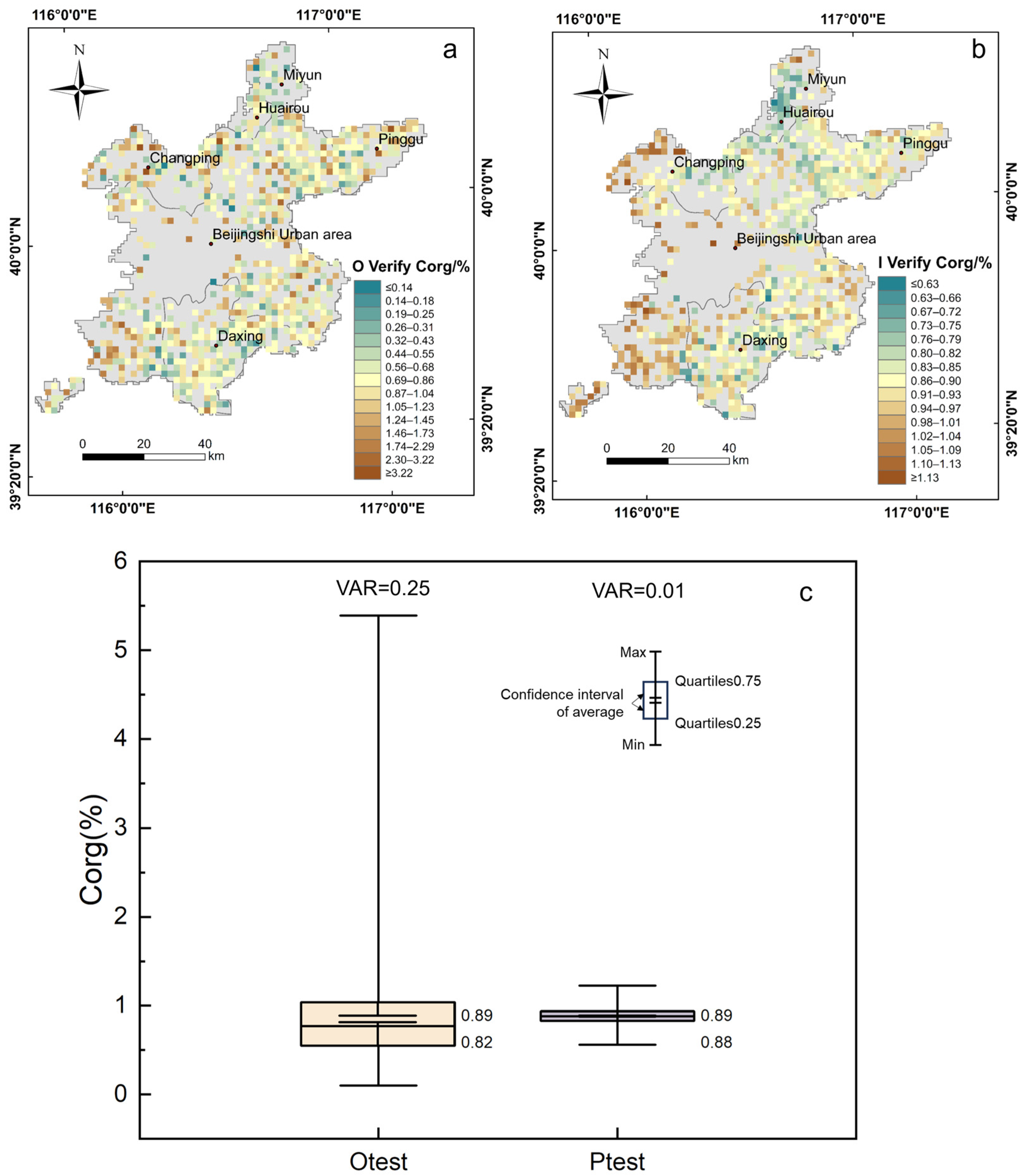
The inferred SOC content for the year 2010 was validated against observed values in the validation area, Beijing, as shown in Figure 7. The observed SOC content shows relatively high concentrations in the southwestern and southeastern parts of Beijing’s urban area, as well as in the northern part of the Changping District and in the Pinggu District. These relatively high concentrations were generally captured in the inferred results. However, in the southeastern part of Beijing’s urban area, the inferred high-value areas did not align well with the observed values. In the southwestern part of Beijing’s urban area, the inferred high-value area was larger than the observed high-value area. In the northern part of Beijing’s urban area and in the Daxing District, the observed SOC content was at a moderate level, which aligned well with the inferred values. In the Miyun District, the SOC content in cropland was generally low, although a few cropland areas exhibited relatively high values. The inferred value also indicated low SOC levels in Daxing cropland, with some scattered high-value points. However, the spatial locations of these inferred high values did not fully match the observed data. From the perspective of each administrative district, the model performs poorly in inferred extreme values, narrowing the range of SOC. The variance between inferred and observed values in Tianjin is the largest, lowering the overall performance. Overall, the model was able to capture the relative spatial distribution of SOC content; however, discrepancies remained in the inference of absolute values.

Figure 7. Predicted and observed spatial distributions of SOC content. (a) Inferred, (b) Observed; (c) The variance and confidence interval of the observed and inferred values in each area.

Quantitatively, the mean observed SOC content in cropland within the validation area in 2010 was 0.85%, compared to an inferred mean of 0.88%. It can be seen in Figure 7c that during validation, the inferred data inherited the characteristics observed in 2000: the actual maximum value is much greater than the inferred maximum, and the inferred range is narrower than the observed range. This indicates that the model can only capture part of the relative spatiotemporal distribution but is limited in terms of absolute values.

3.2. SOC Distribution in Unsampled Periods

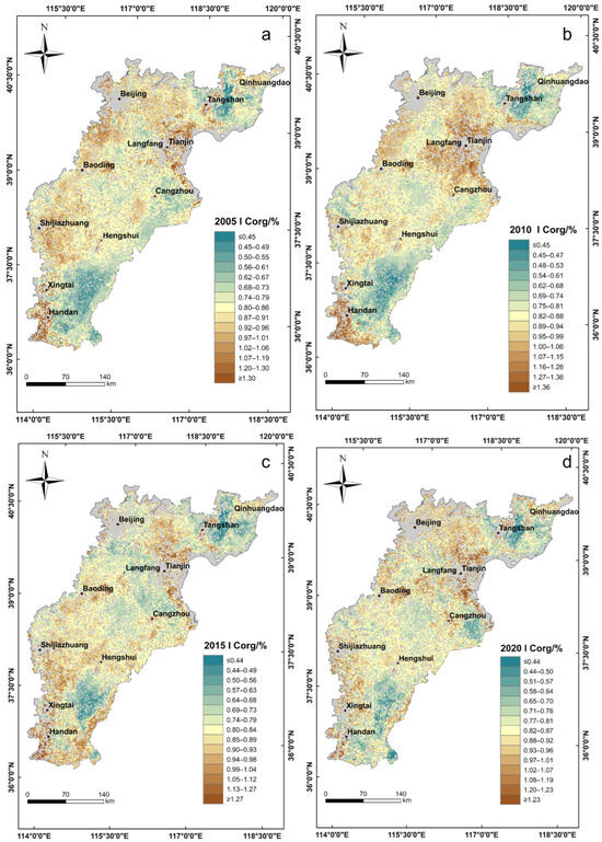
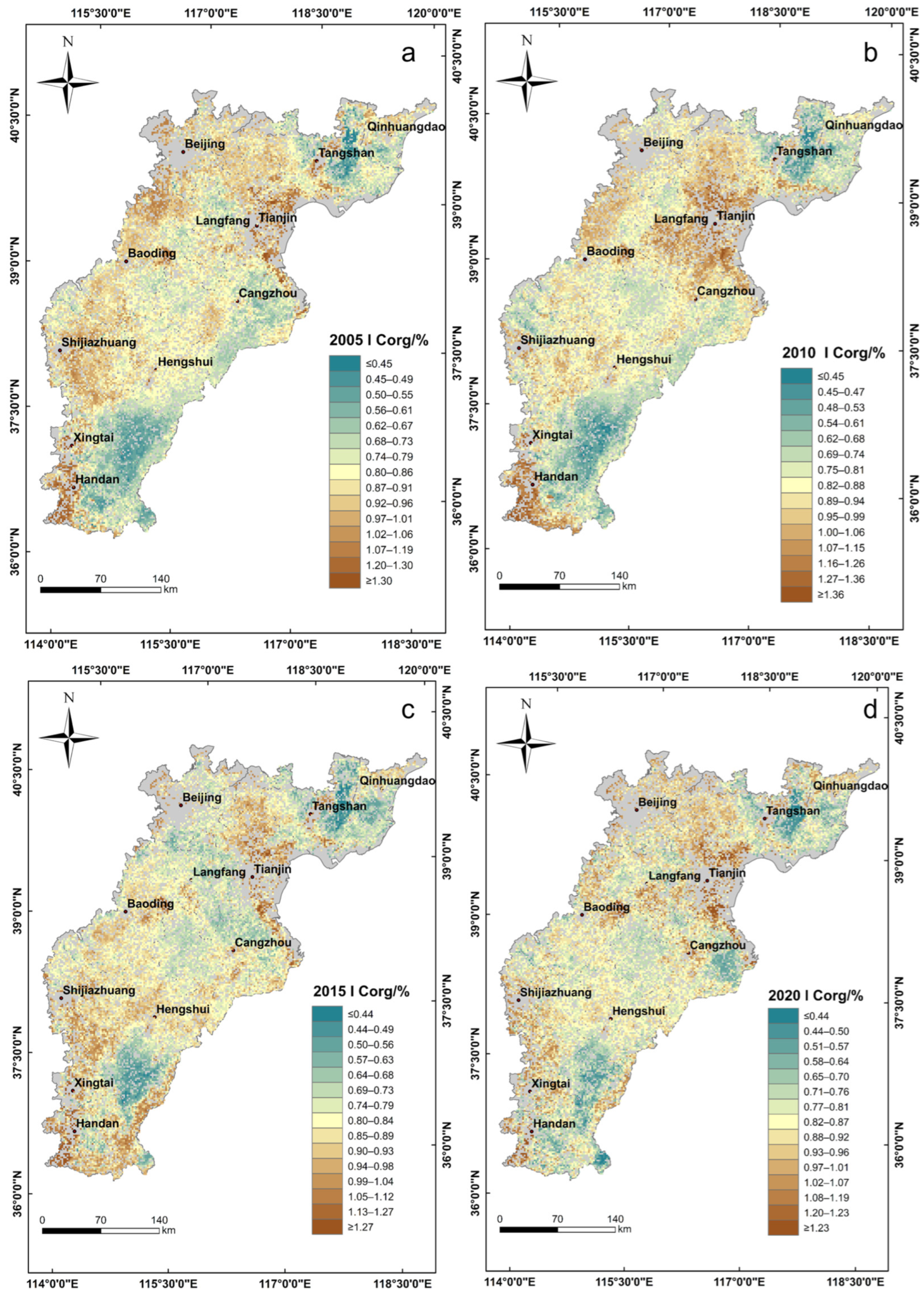
After constructing the inference model of SOC, we obtained the SOC distribution in cropland of the BTH region using this inference model, as shown in Figure 8. The model that passed the robustness evaluation was applied to the entire research area from 2005 to 2020 to obtain the spatiotemporal dynamics of SOC. Regions with significant changes in SOC content were mainly located along the Beijing–Tianjin area and near Handan and Xingtai. The primary low-value areas were distributed to the east of Xingtai and Handan, as well as around Tangshan and Qinhuangdao.

Figure 8. 2005–2020 SOC distribution in cropland of the research area. (a) 2005, (b) 2010, (c) 2015, (d) 2020.

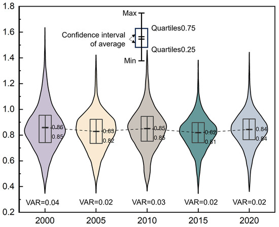
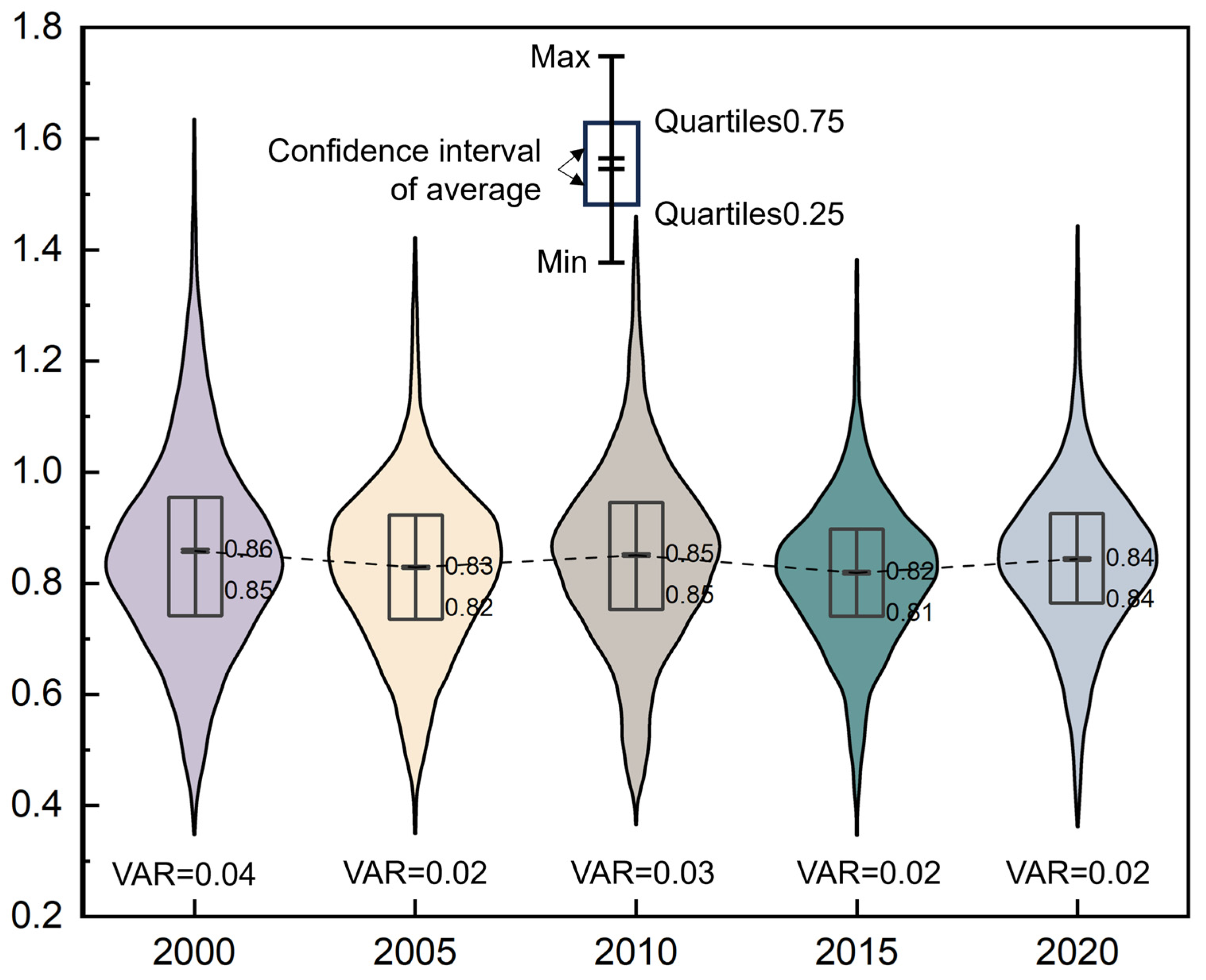
Based on the inferred spatial distribution in each time period, the average SOC content was calculated, as shown in Figure 9. From 2000 to 2020, the overall SOC content in the research area showed a declining trend; however, the decrease was not significant. The average SOC content was 0.86% in 2000 and 0.84% in 2020, representing a slight reduction of only 0.02%, with limited impact on the overall level. The cropland SOC in the research area acted as a carbon source.

Figure 9. The change in average SOC in cropland of research area. Note: For comparison among inferred SOC values, the SOC in 2000 was also represented by inference values. The dashed line represents the trend of the mean SOC change.

4. Discussion

4.1. Comparison with a Baseline Model and Interpretation of Model Performance

To evaluate the advantages of the LightGBM model relative to a baseline model and to verify the necessity of machine learning in this study, multiple linear regression (MLR) was further introduced as the baseline model. Using the same input variables and the same training/testing dataset partition, the predictive performance of the two models was compared, as shown in Table 2.

Table 2. Comparison of model performance.

Model	R2 (Train)	R2 (Test)	RMSE (Train)	RMSE (Test)
lightGBM	0.64	0.45	0.61	0.68
MLR	0.15	0.17	0.93	0.87

The results show that the R² values of MLR for the training and testing datasets are 0.15 and 0.17, respectively, which are significantly lower than the corresponding values of 0.64 and 0.45 obtained by the LightGBM model. This indicates that, under the current environmental factors system, the relationships between SOC and the predictor variables are not simple linear relationships. The LightGBM model is able to capture more complex nonlinear patterns and therefore demonstrates stronger predictive capability than the simple linear model.

Although the LightGBM model shows better performance than the baseline model, the R² of the testing dataset is still only 0.45. This indicates that the currently included environmental variables alone cannot fully explain the spatial variability of SOC. A possible reason is that SOC distribution is influenced not only by environmental factors but also by human management practices, such as irrigation, fertilization, cropping methods, and straw return. However, these management factors usually lack continuous and high-quality raster datasets at the regional scale. As a result, they were not included as model inputs, which may limit the model’s ability to further explain the variability of SOC.

The uncertainties in this study mainly arise from several aspects. First, SOC data were obtained using composite samples, which may smooth small-scale spatial variability, although it reduces local noise. Second, remote sensing data were resampled to match the spatial scale of the SOC data, which may weaken local heterogeneity. Finally, the SOC distribution is influenced by both environmental and human management factors, whereas the current model mainly includes environmental variables, which may limit its explanatory power.

In addition, regularization strategies were applied during model construction to control model complexity and reduce the risk of overfitting. However, a performance gap still exists between the training and testing datasets of the LightGBM model, indicating that its generalization ability remains limited. Besides model complexity, this difference may also be related to the strong spatial heterogeneity of SOC in agricultural areas, the lack of local management information, and uncertainties in the samples themselves. Therefore, the model is considered feasible for SOC inference in unsampled years and performs significantly better than a simple linear model, although its inference accuracy and applicability are still constrained by the input variable system and associated uncertainties.

4.2. Performance of the SOC Inference Model in Comparison with Previous Studies

The performance of the SOC inference model developed in this study is comparable to, and in some cases exceeds, that reported in previous large-scale SOC mapping studies based on machine learning approaches. For example, Dharumarajan et al. reported an R² of approximately 0.31 and an RMSE of around 1.0 for the prediction of SOC at a depth of 15–20 cm on the test set [29]. Similarly, de Brogniez et al. reported an R² of 0.29 for topsoil SOC prediction on the training set and 0.27 on the test set, with the RMSE of the test set ranging from 0.96 to 3.20 [30]. Wang et al. reported that the R² of their model on the test set ranged from 0.12 to 0.28, while the RMSE ranged from 4.03 to 12.03 [31]. These results indicate that the predictive accuracy of the model developed in this study is higher than that reported in some comparable studies, suggesting that it is sufficiently reliable for practical application.

In comparison, the SOC inference model presented in this study achieved an R² of 0.45 on the test set, with a corresponding RMSE of 0.73. These results indicate that, under similar modeling frameworks and data constraints, the predictive performance of the present model is within the upper range of reported values. This may be partly attributed to the integration of season-based crop rotation variables, which provide additional information on vegetation dynamics that is not captured when vegetation is treated as a single annual indicator.

4.3. Relationship Patterns Between SOC and Environmental Factors

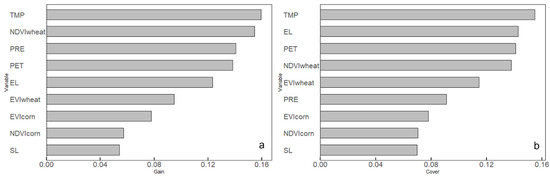
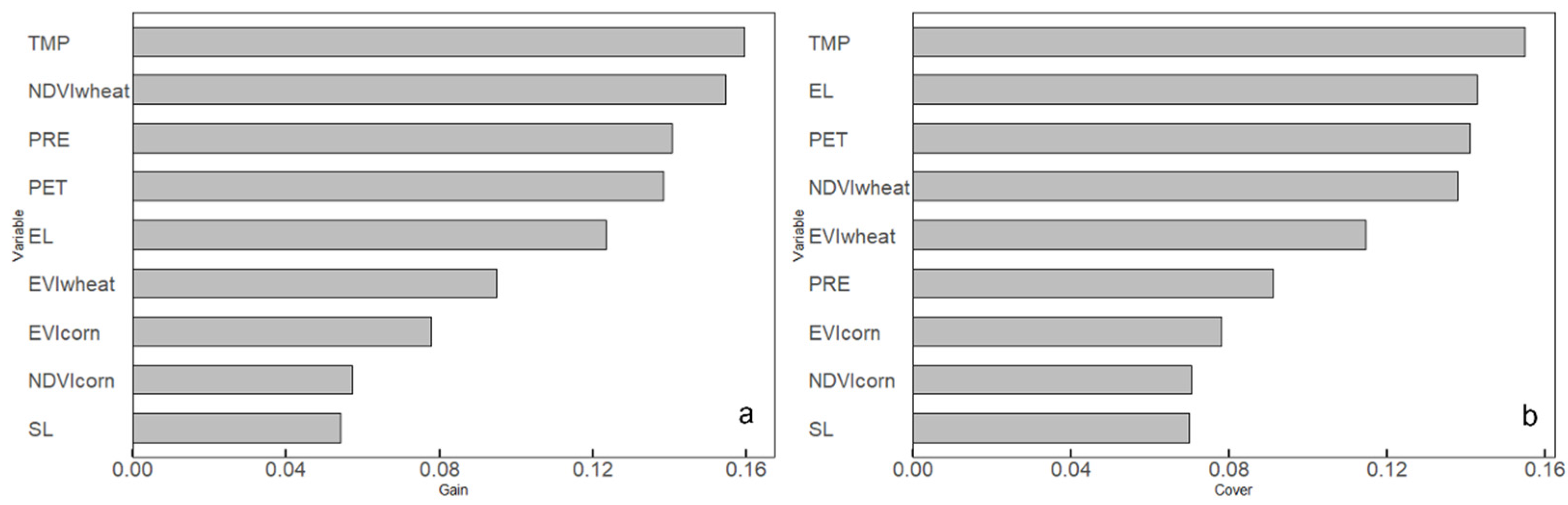
The importance of environmental factors in explaining the spatial distribution of SOC can be partly represented by their rankings in the inference model. Figure 10a shows the Gain of the model, whereas Figure 10b shows the Cover of the model.

Figure 10. The contribution of environmental factors to spatial distribution of SOC. (a) Gain, (b) Cover.

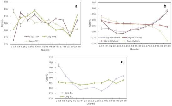
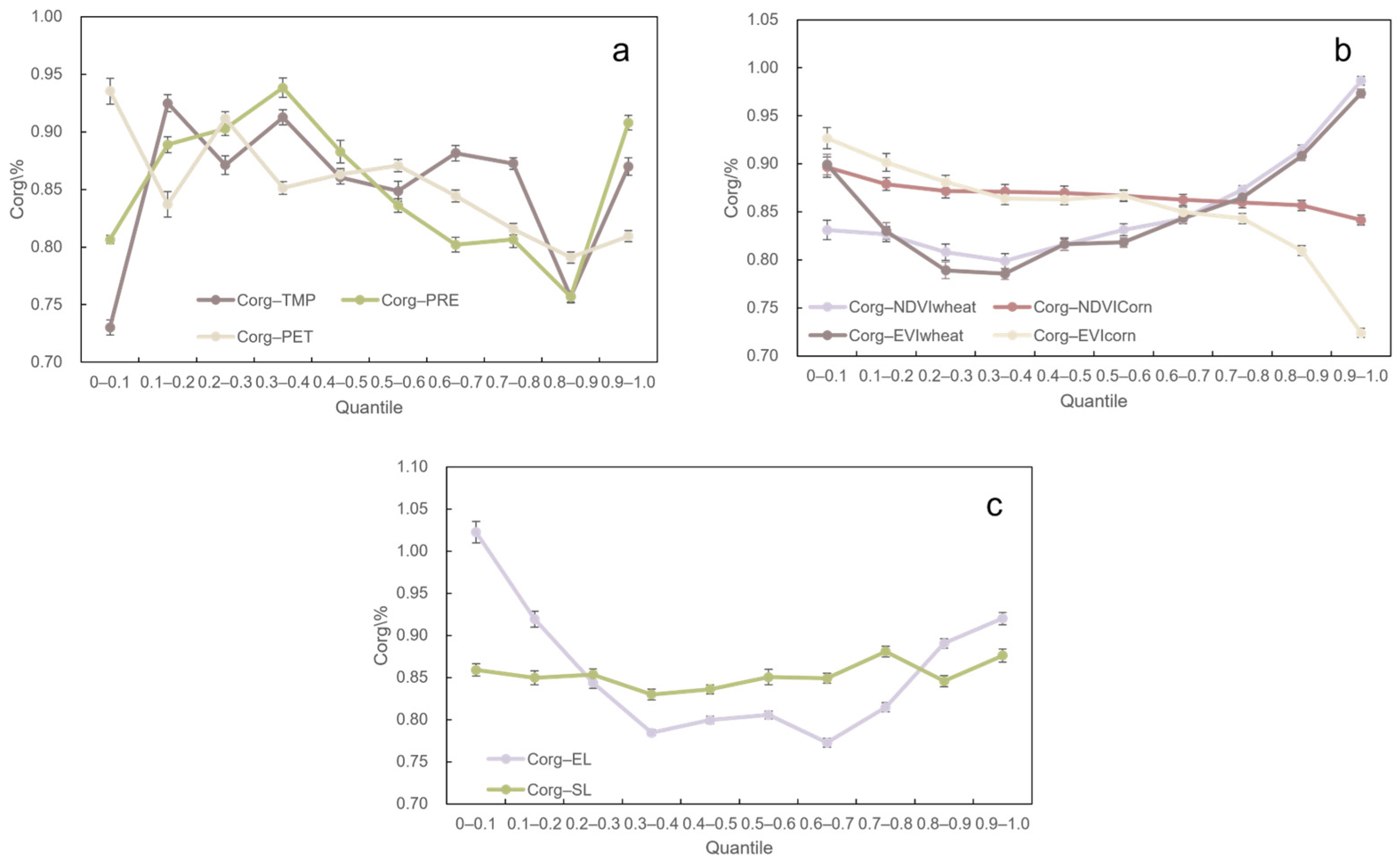
To explore the correlations between SOC and environmental factors, the mean SOC values across different quantiles of each environmental variable were analyzed. This approach effectively displays the relationship between the two variables more clearly, providing an intuitive means of understanding their association [32]. In this study, deciles (10 quantiles) were used to represent the distribution. Table 3 presents the specific values of each decile for the environmental variables within the research area.

Table 3. Specific values of each decile for the environmental factors.

Quantiles	TMP (°C)	PRE (mm)	PET (mm)	NDVI Wheat -	NDVI Corn -	EVI Wheat -	EVI Corn -	EL (m)	SL-
0.0	10.33	335.20	73.95	0.10	0.10	0.07	0.07	0.00	0.00
0.1	11.66	387.00	91.25	0.18	0.55	0.11	0.35	4.00	0.09
0.2	12.23	406.20	94.63	0.23	0.61	0.15	0.41	7.00	0.14
0.3	12.88	416.50	97.26	0.29	0.66	0.19	0.45	10.00	0.18
0.4	13.16	426.60	98.29	0.35	0.69	0.24	0.49	16.00	0.22
0.5	13.30	440.10	98.72	0.41	0.72	0.29	0.52	22.00	0.27
0.6	13.40	461.60	99.07	0.48	0.75	0.34	0.54	28.00	0.33
0.7	13.48	477.50	99.39	0.55	0.77	0.39	0.57	35.00	0.44
0.8	13.62	506.00	99.80	0.62	0.79	0.45	0.60	43.00	0.65
0.9	13.76	567.60	100.26	0.69	0.81	0.52	0.64	60.00	1.49
1.0	14.56	665.60	102.44	0.89	0.90	0.71	0.84	406.00	49.40

Based on the decile grouping of each environmental factor, the mean SOC value within each decile group was calculated and is presented in Figure 11 to illustrate the overall trend of SOC along environmental gradients. Error bars represent the standard error (SE) of the mean SOC within each decile group.

Figure 11. The correlation between SOC and environmental variables. (a) Climate, (b) Vegetation, (c) Terrain. Note: The x-axis represents the deciles of the climatic factors, and the y-axis represents the mean SOC within each decile.

From the perspective of climate, TMP, PRE, and PET all show a negative correlation with SOC content across the study area. As shown in Figure 10, among the climate variables, TMP is identified as the most important factor influencing SOC accumulation. The loss of SOC induced by climate warming may be attributed to increased microbial activity, which accelerates the decomposition of organic matter [33]. Feng et al. suggested that the negative correlation between PRE and SOC may be attributed to SOC loss caused by soil runoff [34]. PET can, to some extent, represent the intensity of soil respiration. Stronger soil respiration indicates higher microbial activity, which in turn accelerates the decomposition of SOC and leads to its loss [35,36]. However, starting from the 0.8 quantile—when the mean TMP exceeds 13.62 °C, PRE exceeds 506 mm, and mean annual PET exceeds 99.80—the relationship between climatic variables and SOC in the research area shifts to a positive correlation, as shown in Figure 11. The potential reason is that higher TMP and PRE promote plant growth, and the increased plant inputs and litter decomposition may compensate for SOC loss, thereby contributing to a net accumulation of SOC [37].

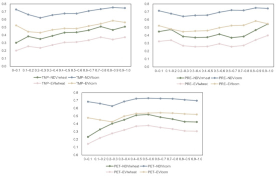
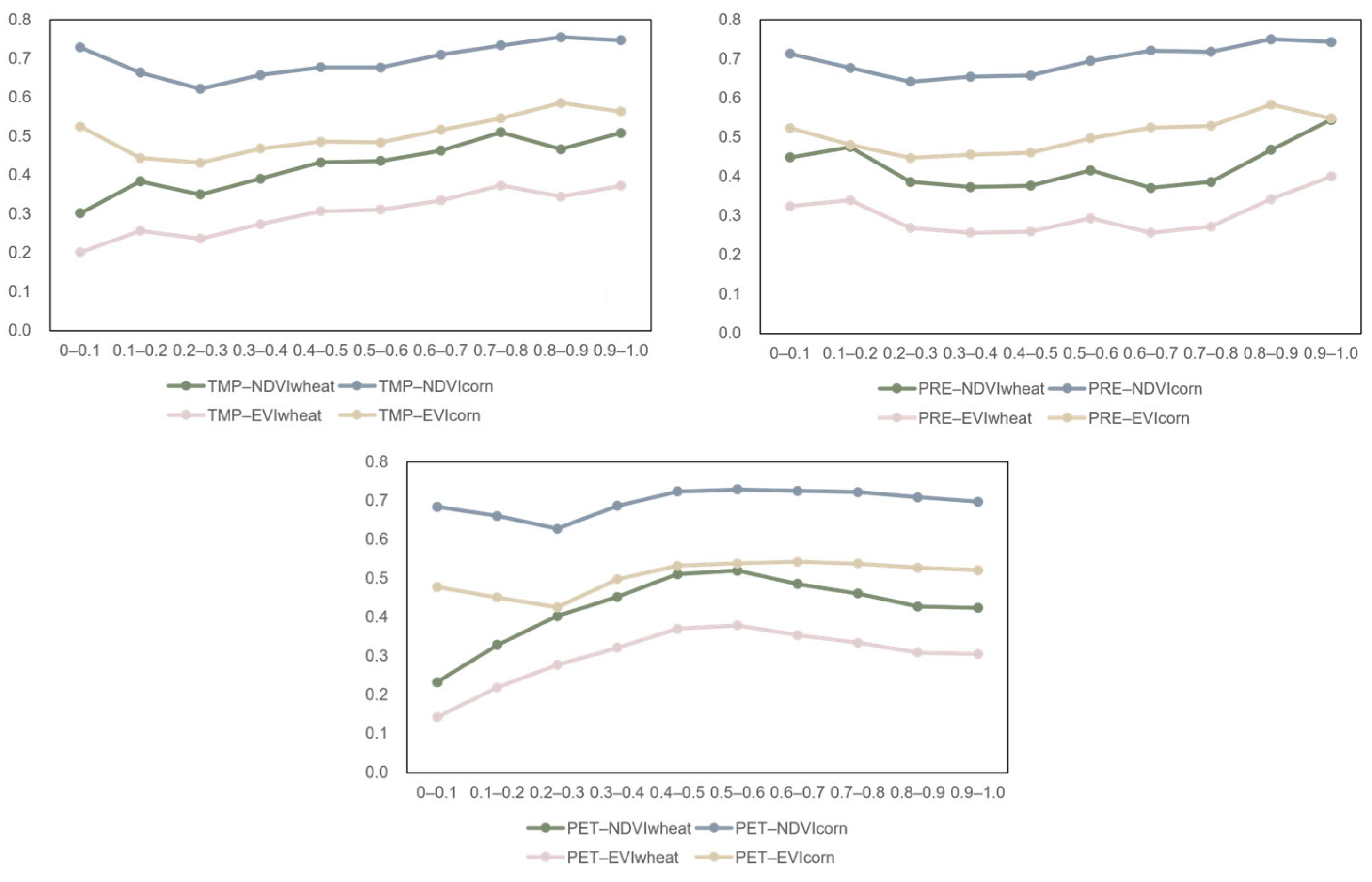
From the perspective of crop rotation, the importance of wheat growth, as reflected in both NDVI and EVI, is greater than that of corn in both model construction and optimization. In the research area, when the quantile exceeds 0.3, SOC content tends to increase as wheat growth improves. However, corn growth does not show a significant correlation with SOC content; in some areas with vigorous corn growth, SOC content may even decrease. The phenomenon of declining SOC content despite vigorous vegetation growth is consistent with the findings of Spohn et al. and may be attributed to inappropriate soil management practices such as fertilization [38]. This suggests that the current management practices for corn cultivation in the research area may need to be adjusted. Although NDVIwheat contributed substantially during model construction, vegetation variables were less influential than climatic variables during the optimization process. This may be due to the relatively uniform crop growth conditions across the study area’s farmland, which limited the additional information that vegetation indicators could provide during model optimization. Meanwhile, the relationship between climate and crops can be used as a reference, as shown in Figure 12. The TMP has a positive relationship with all vegetation factors.

Figure 12. Relationship between vegetation and climate.

From the perspective of terrain, EL consistently showed greater importance than SL in both the construction and optimization of the inference model. SL was the least important variable throughout both stages of the modeling process. The research area is located in a plain region, where slope variation is minimal, which may explain the low importance of slope. This suggests that even in areas with little change in slope, variations in EL can still play a significant role in SOC accumulation and should not be overlooked. From the correlation between EL and SOC content, SOC decreases with increasing EL before the 0.4 quantile but increases with EL beyond this point. This pattern is consistent with the findings of Ma et al., who observed that above a certain EL, SOC content increases with altitude; they suggested that changes in microbial activity associated with increasing elevation are a major factor contributing to the accumulation of SOC [39].

Overall, spatially, the primary factor contributing to SOC accumulation is the growth of wheat during the year. On the other hand, climatic variables play a more important role in the model, with TMP being the most influential climatic factor in both model construction and optimization.

4.4. Estimation of the SOC Level of the Research Area Globally

To evaluate the global level of soil organic carbon density (SOCD) in the research area, we compared it with other regions worldwide. This comparison provides a preliminary indication of whether the SOC in the research area still has potential for further accumulation. SOCD was selected as the comparison indicator because several previous studies reported only SOCD without providing SOC content. In addition, SOCD values are more commonly reported in existing studies. Therefore, we converted SOC content (Corg) into SOCD for comparison, as shown in Equation (4). When selecting previous studies, if specific geographic coordinates of the study area were unavailable, the coordinates of the corresponding country or province were used. If the study area boundaries were clearly defined, the coordinates of the central point of the area were adopted. For studies where SOCD was obtained for other experimental purposes, the SOCD of the control group was used. When multiple samples were collected within the target area, the median SOCD value was used for analysis.

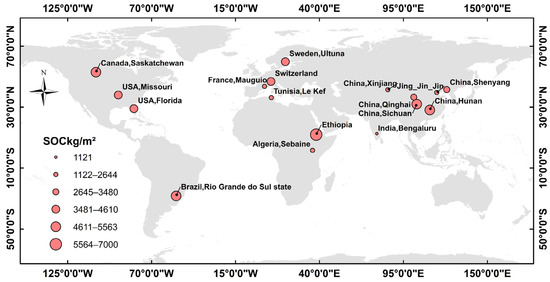
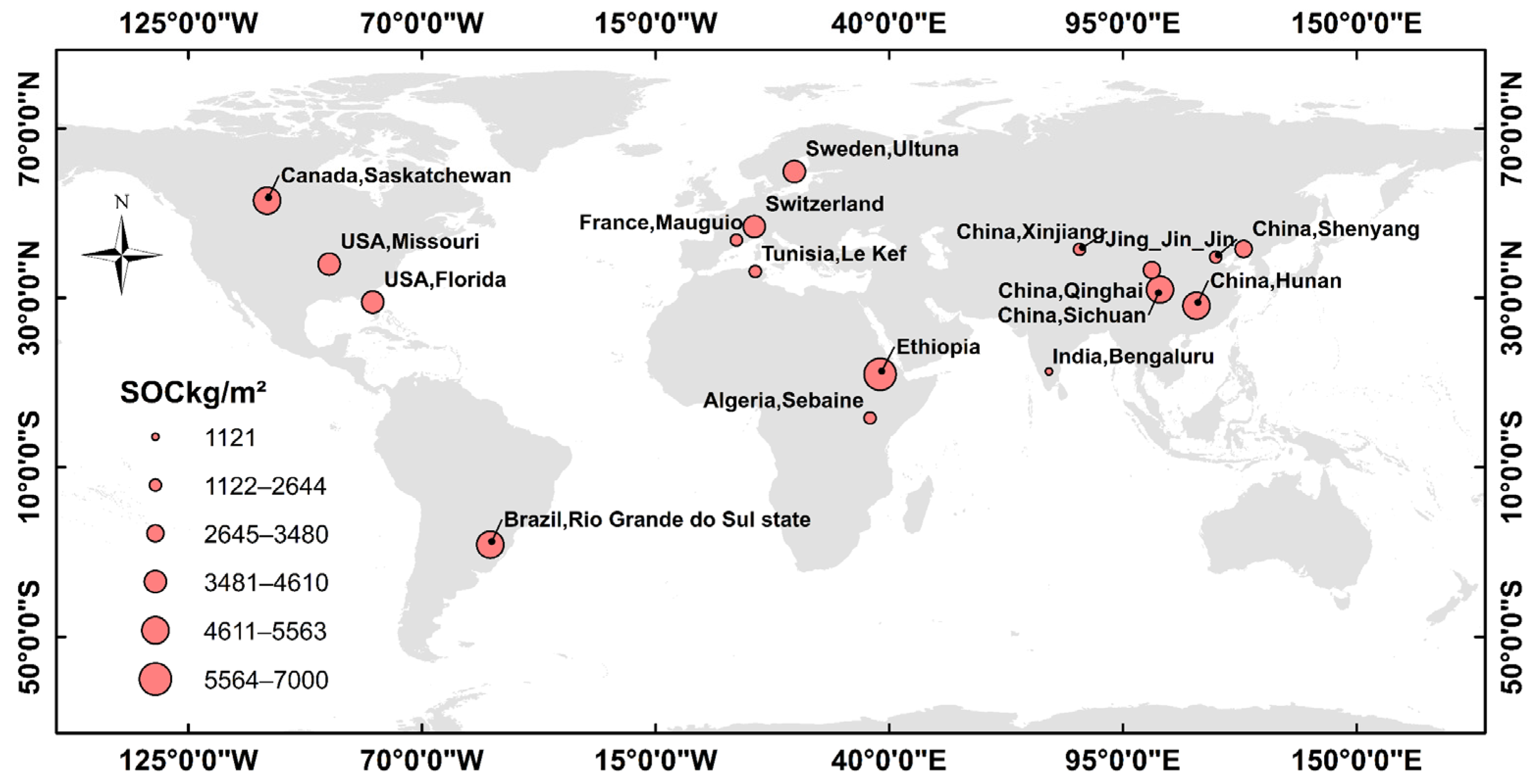
The field sampling results from 2000 show that the average SOCD in the croplands of the BTH region was 2284.97 t/km². The global distribution of SOCD is presented in Figure 13.

Figure 13. Global distribution of SOCD in croplands at 20 cm depth.

From a national perspective, the SOCD in the BTH region is relatively low, and is lower than that in Qinghai, Hunan, Shenyang, and Sichuan [40,41,42,43]; however, it is larger than Xinjiang [44].

From a global perspective, the SOCD in the BTH region is also relatively low, ranking just above that of Tunisia, India, and Algeria [45,46,47], similar to the Mauguio province of France [48] and smaller than other regions [38,39,40,41,42,43,44,45,46,47,48,49,50,51,52,53,54]. Among the previously published data collected in this study, the highest SOCD in cropland was observed in the Ethiopian Highlands, reaching up to 7000 t/km², while the lowest value was found in the Bangalore region of India, with an SOCD of 1121 t/km².

Overall, the SOCD in the BTH region is relatively low both nationally and globally. Compared with Missouri, USA, which shares similar latitude and climatic conditions with an SOCD of 4100 t/km² [50], the BTH region still has significant potential for improvement in its cropland SOCD.

4.5. Limitations and Outlook

The limitations of this study are as follows: First, although environmental factors can partly reflect the spatial distribution of SOC, they cannot represent it entirely. Under the current data conditions, datasets related to fertilization, tillage, and other management practices cannot be matched accurately to raster scales, leading to incomplete data; thus, they cannot be used as predictive variables in the SOC inference model. Second, the available soil property datasets are outdated (measured mainly in the 1960s–1980s) and of low resolution; therefore, they were not included as input parameters in the model but were used only as reference information. Third, the SOC validation dataset used for the Beijing region in 2010 was not derived from original field samples. Similar to previous studies, the datasets that can reliably verify large-scale SOC inference models remain incomplete and require improvement. Finally, as this study established the relationship between environmental factors and SOC based on data from a single period, the results cannot fully represent long-term SOC accumulation. Hence, field sampling at different time periods remains essential. The approach in this research is applied to the extant SOC and environmental factors’ data, uses machine learning to find relationship patterns between them, and makes an inference of SOC distribution in the unsampled periods. The approach applied in this study aims to explore the relationship patterns between SOC and environmental factors using available data and machine learning methods, and to further infer the potential distribution of SOC during unsampled periods based on these patterns. However, this approach represents a potential solution under data-limited conditions and cannot replace field sampling or mechanistic models. Therefore, we will further explore mechanistic models in future research.

5. Conclusions

In this research, we conducted two periods of field sampling in cropland across the southeastern plain of the BTH region. The first sampling campaign was carried out in 2000 and covered the entire study area. Based on these data, we explored the spatial relationship patterns between SOC and environmental factors and assessed the feasibility of inferring potential future SOC changes in cropland. Field sampling data collected from cropland in Beijing in 2010 were used as a reference for comparison with the inferred results. Environmental factors considered in this study included climatic variables, seasonal vegetation growth associated with the crop rotation system, and topographic factors. A LightGBM model was applied to investigate the relationship patterns between SOC and these environmental factors and to evaluate the feasibility of inferring SOC distributions during unsampled periods. Furthermore, SOC distributions for four unsampled years (2005, 2010, 2015, and 2020) were inferred. The results are as follows:

(1)

According to the field sampling results, the average SOC density in the croplands of the BTH region is 2284.97 t/km², which is relatively low globally and comparable to that of France.

(2)

According to the crop rotation system, consistent with our hypothesis, wheat growth showed the strongest positive correlation with SOC content. In contrast, corn growth had little impact on SOC in most cases, and high corn vigor was even associated with a decline in SOC. Therefore, improved fertilization and management strategies for corn are needed in the region.

(3)

According to the other environmental factors, TMP played the most important role among climatic variables in influencing SOC formation in the research area.

(4)

According to the cross-period inferences between environmental factors and SOC, the difference between the inference and observed mean values and confidence intervals in 2000 exceeded 0.3, while all other differences were below 0.1. In the 2010 validation, the difference between the inferred and observed mean values and confidence intervals was also less than 0.1. This indicates that the model can reasonably estimate the overall regional SOC conditions. However, the maximum and minimum values of the inferred and observed SOC in both 2000 and 2010 showed large discrepancies, as the model tended to narrow the range between extremes. Therefore, this method can serve as a reference for SOC inference and cannot replace field sampling activities.

References

- Lal, R. Agricultural Activities and the Global Carbon Cycle. Nutr. Cycl. Agroecosyst. 2004, 70, 103–116. [Google Scholar] [CrossRef] [Scilit]
- Zomer, R.J.; Bossio, D.A.; Sommer, R.; Verchot, L.V. Global Sequestration Potential of Increased Organic Carbon in Cropland Soils. Sci. Rep. 2017, 7, 15554. [Google Scholar] [CrossRef] [Scilit] [PubMed]
- Jia, J.; de Goede, R.; Li, Y.; Zhang, J.; Wang, G.; Zhang, J.; Creamer, R. Unlocking Soil Health: Are Microbial Functional Genes Effective Indicators? Soil Biol. Biochem. 2025, 204, 109768. [Google Scholar] [CrossRef] [Scilit]
- Țopa, D.-C.; Căpșună, S.; Calistru, A.-E.; Ailincăi, C. Sustainable Practices for Enhancing Soil Health and Crop Quality in Modern Agriculture: A Review. Agriculture 2025, 15, 998. [Google Scholar] [CrossRef] [Scilit]
- Yang, R.; Zhu, C.; Zhang, X.; Huang, L. A Preliminary Assessment of the Space-for-Time Substitution Method in Soil Carbon Change Prediction. Soil Sci. Soc. Am. J. 2022, 86, 423–434. [Google Scholar] [CrossRef] [Scilit]
- Zhang, S.; Tian, J.; Lu, X.; Tian, Q. Temporal and Spatial Dynamics Distribution of Organic Carbon Content of Surface Soil in Coastal Wetlands of Yancheng, China from 2000 to 2022 Based on Landsat Images. Catena 2023, 223, 106961. [Google Scholar] [CrossRef] [Scilit]
- Song, X.; Yang, J.; Zhao, M.; Zhang, G.-L.; Liu, F.; Wu, H.-Y. Heuristic Cellular Automaton Model for Simulating Soil Organic Carbon under Land Use and Climate Change: A Case Study in Eastern China. Agric. Ecosyst. Environ. 2019, 269, 156–166. [Google Scholar] [CrossRef] [Scilit]
- Muñoz, A.; Alvis, Á.; Martínez, I. A Random Forest Model to Predict Soil Organic Carbon Storage in Mangroves from Southern Colombian Pacific Coast. Estuar. Coast. Shelf Sci. 2024, 299, 108674. [Google Scholar] [CrossRef] [Scilit]
- Chen, F.; Feng, P.; Harrison, M.T.; Wang, B.; Liu, K.; Zhang, C.; Hu, K. Cropland Carbon Stocks Driven by Soil Characteristics, Rainfall and Elevation. Sci. Total Environ. 2023, 862, 160602. [Google Scholar] [CrossRef] [Scilit]
- Breiman, L. Random Forests. Mach. Learn. 2001, 45, 5–32. [Google Scholar] [CrossRef] [Scilit]
- Chen, T.; Guestrin, C.; Assoc Comp, M. Xgboost: A Scalable Tree Boosting System. In Proceedings of the 22nd ACM SIGKDD International Conference on Knowledge Discovery and Data Mining (KDD), San Francisco, CA, USA, 13–17 August 2016; pp. 785–794. [Google Scholar]
- Ke, G.; Meng, Q.; Finley, T.; Wang, T.; Chen, W.; Ma, W.; Ye, Q.; Liu, T.Y. Lightgbm: A Highly Efficient Gradient Boosting Decision Tree. In Proceedings of the 31st Annual Conference on Neural Information Processing Systems (NIPS), Long Beach, CA, USA, 4–9 December 2017. [Google Scholar]
- Adeniyi, O.D.; Brenning, A.; Maerker, M. Spatial Prediction of Soil Organic Carbon: Combining Machine Learning with Residual Kriging in an Agricultural Lowland Area (Lombardy Region, Italy). Geoderma 2024, 448, 116953. [Google Scholar] [CrossRef] [Scilit]
- Wang, F.; Liang, R.; Li, S.; Xiang, M.; Yang, W.; Lu, M.; Song, Y. Assessing the Impact of Multi-Source Environmental Variables on Soil Organic Carbon in Different Land Use Types of China Using an Interpretable High-Precision Machine Learning Method. Ecol. Indic. 2024, 169, 112865. [Google Scholar] [CrossRef] [Scilit]
- Ou, J.; Wu, Z.; Yan, Q.; Feng, X.; Zhao, Z. Improving Soil Organic Carbon Mapping in Farmlands Using Machine Learning Models and Complex Cropping System Information. Environ. Sci. Eur. 2024, 36, 80. [Google Scholar] [CrossRef] [Scilit]
- Mu, J.; Wang, J.; Liu, B.; Yang, M. Spatiotemporal Dynamics and Influencing Factors of Co2 Emissions under Regional Collaboration: Evidence from the Beijing-Tianjin-Hebei Region in China. Environ. Pollut. 2024, 357, 124403. [Google Scholar] [CrossRef] [Scilit] [PubMed]
- Xu, C.; Lu, C.; Wang, J. Impact of Meteorological Factors on Wheat Growth Period and Irrigation Water Requirement—A Case Study of the Beijing-Tianjin-Hebei Region in China. bioRxiv 2021. [Google Scholar] [CrossRef] [Scilit]
- Yang, Z.; Yu, T.; Hou, Q.; Xia, X.; Feng, H.; Huang, C.; Wang, L.; Lv, Y.; Zhang, M. Geochemical Evaluation of Land Quality in China and Its Applications. J. Geochem. Explor. 2014, 139, 122–135. [Google Scholar] [CrossRef] [Scilit]
- Li, M.; Xi, X.; Xiao, G.; Cheng, H.; Yang, Z.; Zhou, G.; Ye, J.; Li, Z. National Multi-Purpose Regional Geochemical Survey in China. J. Geochem. Explor. 2014, 139, 21–30. [Google Scholar] [CrossRef] [Scilit]
- Xu, M.; Fu, Y.; Pan, W.; Zhou, G.; Sun, W. Exploring Effective Network Design for Monitoring Soil Ph and Potentially Toxic Elements Based on Geochemical Surveys in Economically Developed Area. Environ. Geochem. Health 2023, 45, 9709–9725. [Google Scholar] [CrossRef] [Scilit]
- Yu, T.; Fu, Y.; Hou, Q.; Xia, X.; Yan, B.; Yang, Z. Soil Organic Carbon Increase in Semi-Arid Regions of China from 1980s to 2010s. Appl. Geochem. 2020, 116, 104575. [Google Scholar] [CrossRef] [Scilit]
- Yang, J.; Huang, X. The 30 M Annual Land Cover Dataset and Its Dynamics in China from 1990 to 2019. Earth Syst. Sci. Data 2021, 13, 3907–3925. [Google Scholar] [CrossRef] [Scilit]
- Nachtergaele, F.; Van Velthuizen, H.; Verelst, L.; Batjes, N.; Dijkshoorn, K.; van Engelen, V.; Fischer, G.; Jones, A.; Montanarella, L.; Petri, M.; et al. Harmonized World Soil Database. In Proceedings of the 19th World Congress of Soil Science, Soil Solutions for a Changing World; International Union of Soil Sciences: Brisbane, Australia, 2010. [Google Scholar]
- Yao, R.; Zhang, Y.; Wang, L.; Li, J.; Yang, Q. Reconstructed Ndvi and Evi Datasets in China (Revichina) Generated by a Spatial-Interannual Reconstruction Method. Int. J. Digit. Earth 2023, 16, 4749–4768. [Google Scholar]
- Peng, S. 1-Km Monthly Precipitation Dataset for China (1901–2024); National Tibetan Plateau Data Center: Beijing, China, 2020. [Google Scholar] [CrossRef]
- Peng, S. 1-Km Monthly Mean Temperature Dataset for China (1901–2024); Edited by Center, National Tibetan Plateau/Third Pole Environment Data, 2019. Available online: https://data.tpdc.ac.cn/en/data/71ab4677-b66c-4fd1-a004-b2a541c4d5bf/ (accessed on 1 January 2026).
- Peng, S. 1-Km Monthly Potential Evapotranspiration Dataset for China (1901–2024). Edited by Center, National Tibetan Plateau/Third Pole Environment Data, 2022. Available online: https://loess.geodata.cn/data/datadetails.html?dataguid=34595274939620&docid=74 (accessed on 1 January 2026).
- Farr, T.G.; Rosen, P.A.; Caro, E.; Crippen, R.; Duren, R.; Hensley, S.; Kobrick, M.; Paller, M.; Rodriguez, E.; Roth, L.; et al. The Shuttle Radar Topography Mission. Rev. Geophys. 2007, 45, RG2004. [Google Scholar] [CrossRef] [Scilit]
- Dharumarajan, S.; Kalaiselvi, B.; Suputhra, A.; Lalitha, M.; Vasundhara, R.; Kumar, K.A.; Nair, K.; Hegde, R.; Singh, S.; Lagacherie, P. Digital Soil Mapping of Soil Organic Carbon Stocks in Western Ghats, South India. Geoderma Reg. 2021, 25, e00387. [Google Scholar] [CrossRef] [Scilit]
- de Brogniez, D.; Ballabio, C.; Stevens, A.; Jones, R.J.A.; Montanarella, L.; van Wesemael, B. A Map of the Topsoil Organic Carbon Content of Europe Generated by a Generalized Additive Model. Eur. J. Soil Sci. 2014, 66, 121–134. [Google Scholar] [CrossRef] [Scilit]
- Wang, T.; Zhou, W.; Xiao, J.; Li, H.; Yao, L.; Xie, L.; Wang, K. Soil Organic Carbon Prediction Using Sentinel-2 Data and Environmental Variables in a Karst Trough Valley Area of Southwest China. Remote Sens. 2023, 15, 2118. [Google Scholar] [CrossRef] [Scilit]
- Gashu, G.; Awoke, H. Effect of Environmental Gradient on Organic Carbon Stock of Wacho Forest Soil, South Western Ethiopia. Proc. Natl. Acad. Sci. India Sect. A Phys. Sci. 2023, 94, 11–15. [Google Scholar] [CrossRef] [Scilit]
- Prietzel, J.; Zimmermann, L.; Schubert, A.; Christophel, D. Organic Matter Losses in German Alps Forest Soils since the 1970s Most Likely Caused by Warming. Nat. Geosci. 2016, 9, 543–548. [Google Scholar] [CrossRef] [Scilit]
- Feng, Y.; Xiao, J.; Wei, Y.; Cai, H.; Yu, J. Large Macroaggregate Disintegration Contributes to Cpom Transfer and Carbon Loss in Forest Soil under Rainfall Simulation. J. Soils Sediments 2022, 23, 777–791. [Google Scholar] [CrossRef] [Scilit]
- Yang, X.; Wang, M.; Huang, Y.; Wang, Y. A One-Compartment Model to Study Soil Carbon Decomposition Rate at Equilibrium Situation. Ecol. Model. 2002, 151, 63–73. [Google Scholar] [CrossRef] [Scilit]
- Lohila, A.; Aurela, M.; Regina, K.; Laurila, T. Soil and Total Ecosystem Respiration in Agricultural Fields: Effect of Soil and Crop Type. Plant Soil. 2003, 251, 303–317. [Google Scholar] [CrossRef] [Scilit]
- Chalchissa, F.B.; Kuris, B.K. Modelling Soil Organic Carbon Dynamics under Extreme Climate and Land Use and Land Cover Changes in Western Oromia Regional State, Ethiopia. J. Environ. Manage. 2024, 350, 119598. [Google Scholar] [CrossRef] [Scilit] [PubMed]
- Spohn, M.; Braun, S.; Sierra, C.A. Continuous Decrease in Soil Organic Matter Despite Increased Plant Productivity in an 80-Years-Old Phosphorus-Addition Experiment. Commun. Earth Environ. 2023, 4, 251. [Google Scholar] [CrossRef] [Scilit]
- Ma, H.-P.; Yang, X.-L.; Guo, Q.-Q.; Zhang, X.-J.; Zhou, C.-N. Soil Organic Carbon Pool Along Different Altitudinal Level in the Sygera Mountains, Tibetan Plateau. J. Mt. Sci. 2016, 13, 476–483. [Google Scholar] [CrossRef] [Scilit]
- Zhang, Y.; Cai, X.; Lv, J. Size and Dynamics of Soil Organic Carbon Stock in Cropland of the Eastern Qinghai-Tibetan Plateau. Agric. Ecosyst. Environ. 2016, 222, 125–132. [Google Scholar] [CrossRef] [Scilit]
- Lou, Y.; Xu, M.; Wang, W.; Sun, X.; Liang, C. Soil Organic Carbon Fractions and Management Index after 20 Yr of Manure and Fertilizer Application for Greenhouse Vegetables. Soil Use Manage. 2011, 27, 163–169. [Google Scholar] [CrossRef] [Scilit]
- Tang, H.; Li, C.; Xiao, X.; Pan, X.; Cheng, K.; Shi, L.; Li, W.; Wen, L.; Wang, K. Effects of Long-Term Fertiliser Regime on Soil Organic Carbon and Its Labile Fractions under Double Cropping Rice System of Southern China. Acta Agric. Scand. Sect. B—Soil Plant Sci. 2020, 70, 409–418. [Google Scholar] [CrossRef] [Scilit]
- Li, S.; Zhang, S.; Pu, Y.; Li, T.; Xu, X.; Jia, Y.; Deng, O.; Gong, G. Dynamics of Soil Labile Organic Carbon Fractions and C-Cycle Enzyme Activities under Straw Mulch in Chengdu Plain. Soil Tillage Res. 2016, 155, 289–297. [Google Scholar] [CrossRef] [Scilit]
- Shan, Y.; Li, G.; Bai, Y.; Liu, H.; Zhang, J.; Wei, K.; Wang, Q.; Wu, B.; Cao, L. Effects of Different Improvement Measures on Hydrothermal Carbon and Cotton (Gossypium hirsutum L.) Yield in Saline-Alkali Soil. Appl. Ecol. Environ. Res. 2022, 20, 1821–1835. [Google Scholar] [CrossRef] [Scilit]
- Salima, B.; Fatiha, F.; Karima, O. Incidence of Manure Amendment on Soil Organic Carbon Stock under Semi-Arid Environment. Fresenius Environ. Bull. 2022, 31, 10892–10902. [Google Scholar]
- Jaziri, S.; M’Hamed, H.C.; Rezgui, M.; Labidi, S.; Souissi, A.; Rezgui, M.; Barbouchi, M.; Annabi, M.; Bahri, H. Long Term Effects of Tillage-Crop Rotation Interaction on Soil Organic Carbon Pools and Microbial Activity on Wheat-Based System in Mediterranean Semi-Arid Region. Agronomy 2022, 12, 953. [Google Scholar] [CrossRef] [Scilit]
- Prasad, J.; Rao, C.S.; Srinivas, K.; Jyothi, C.N.; Venkateswarlu, B.; Ramachandrappa, B.; Dhanapal, G.; Ravichandra, K.; Mishra, P. Effect of Ten Years of Reduced Tillage and Recycling of Organic Matter on Crop Yields, Soil Organic Carbon and Its Fractions in Alfisols of Semi Arid Tropics of Southern India. Soil Tillage Res. 2016, 156, 131–139. [Google Scholar] [CrossRef] [Scilit]
- Siegwart, L.; Piton, G.; Jourdan, C.; Piel, C.; Sauze, J.; Sugihara, S.; Bertrand, I. Carbon and Nutrient Colimitations Control the Microbial Response to Fresh Organic Carbon Inputs in Soil at Different Depths. Geoderma 2023, 440, 116729. [Google Scholar] [CrossRef] [Scilit]
- Ross, C.W.; Grunwald, S.; Myers, D.B. Spatiotemporal Modeling of Soil Organic Carbon Stocks across a Subtropical Region. Sci. Total Environ. 2013, 461–462, 149–157. [Google Scholar] [CrossRef] [Scilit] [PubMed]
- Eynard, A.; Schumacher, T.; Lindstrom, M.; Malo, D. Effects of Agricultural Management Systems on Soil Organic Carbon in Aggregates of Ustolls and Usterts. Soil Tillage Res. 2005, 81, 253–263. [Google Scholar] [CrossRef] [Scilit]
- Bruni, E.; Guenet, B.; Clivot, H.; Kätterer, T.; Martin, M.; Virto, I.; Chenu, C. Defining Quantitative Targets for Topsoil Organic Carbon Stock Increase in European Croplands: Case Studies with Exogenous Organic Matter Inputs. Front. Environ. Sci. 2022, 10, 824724. [Google Scholar] [CrossRef] [Scilit]
- Abegaz, A.; Winowiecki, L.A.; Vågen, T.-G.; Langan, S.; Smith, J.U. Spatial and Temporal Dynamics of Soil Organic Carbon in Landscapes of the Upper Blue Nile Basin of the Ethiopian Highlands. Agric. Ecosyst. Environ. 2016, 218, 190–208. [Google Scholar] [CrossRef] [Scilit]
- Bortolon, E.S.O.; Mielniczuk, J.; Tornquist, C.G.; Lopes, F.; Bergamaschi, H. Validation of the Century Model to Estimate the Impact of Agriculture on Soil Organic Carbon in Southern Brazil. Geoderma 2011, 167–168, 156–166. [Google Scholar] [CrossRef] [Scilit]
- Sorenson, P.T.; Bedard-Haughn, A.K.; Luce, M.S. Combining Predictive Soil Mapping and Process Models to Estimate Future Carbon Sequestration Potential under No-Till. Can. J. Soil Sci. 2024, 104, 469–481. [Google Scholar] [CrossRef] [Scilit]
Disclaimer/Publisher’s Note: The statements, opinions and data contained in all publications are solely those of the individual author(s) and contributor(s) and not of MDPI and/or the editor(s). MDPI and/or the editor(s) disclaim responsibility for any injury to people or property resulting from any ideas, methods, instructions or products referred to in the content. |
© 2026 by the authors. Licensee MDPI, Basel, Switzerland. This article is an open access article distributed under the terms and conditions of the Creative Commons Attribution (CC BY) license.