


Abstract
Global Navigation Satellite Systems (GNSS) positioning accuracy is affected by multiple error sources, including atmospheric delays, multipath propagation, and receiver noise, which can significantly reduce positioning reliability in low-cost receivers. This study investigates the use of a feedforward neural network to compensate for positioning errors in a static GNSS receiver scenario. A synthetic dataset was generated in MATLAB/Simulink by simulating positioning perturbations around a known reference location. Consecutive coordinate differences were used as input features, and a compact feedforward neural network with 45 hidden neurons was trained using the Levenberg–Marquardt algorithm to estimate positioning error components. The proposed approach was evaluated through residual error distribution, regression, temporal dispersion, and spatial scatter analyses. The results indicate that, for the primary 10 m error scenario, neural network-based compensation reduced temporal dispersion by approximately 46% and produced a more compact spatial distribution of corrected positions around the reference location. The residual errors remained concentrated near zero, indicating improved positioning consistency under the investigated simulation conditions. Sensitivity analysis across nominal error radii of = 1, 5, 10, 15, and 20 m showed consistent reductions in both RMSE and standard deviation for radii of 10 m and above, whereas no consistent improvement was observed at lower error levels. In a preliminary comparison with random forests, XGBoost, Long Short-Term Memory (LSTM), and Gated Recurrent Unit models using the same training, validation, and test samples, the Feedforward Neural Network (FNN) achieved competitive test MSE while requiring substantially less training time and runtime memory than the LSTM. These findings support the proof-of-concept feasibility of lightweight FNN-based correction for simulated static GNSS positioning. Future work will focus on validation using real GNSS measurements and extension to dynamic positioning applications.
1. Introduction
Global Navigation Satellite Systems (GNSS), including the Global Positioning System (GPS), GLONASS, Galileo, and BeiDou, have become indispensable technologies for positioning, navigation, and timing applications across numerous scientific, industrial, environmental, and engineering domains [1]. Their widespread adoption has been facilitated by the increasing availability of low-cost receivers, the expansion of multi-constellation services, and the growing demand for location-aware systems in areas such as intelligent transportation, precision agriculture, geodesy, autonomous platforms, infrastructure monitoring, and Internet of Things (IoT) applications, and nanosatellite missions requiring autonomous onboard processing and reliable positioning capabilities [1,2]. Despite these advances, the positioning performance of low-cost GNSS receivers remains significantly affected by a variety of error sources, including satellite orbit and clock inaccuracies, ionospheric and tropospheric propagation delays, multipath propagation, non-line-of-sight (NLOS) reception, signal blockage, receiver noise, and local environmental conditions [3,4,5,6,7,8]. These factors often lead to degraded positioning accuracy and reduced stability of the estimated coordinates, particularly in challenging operating environments.
To mitigate such errors, numerous positioning enhancement techniques have been developed over the past decades. Differential GNSS, Real-Time Kinematic (RTK), and Precise Point Positioning (PPP) are among the most widely adopted approaches for improving positioning accuracy beyond the capabilities of standalone GNSS receivers [9,10,11,12]. RTK positioning achieves centimetre-level accuracy by resolving carrier-phase ambiguities using observations from nearby reference stations, while PPP exploits precise satellite orbit and clock products to achieve decimetre-level positioning without local infrastructure. Furthermore, Kalman-filter-based estimation frameworks remain fundamental components of modern navigation systems and Global Navigation Satellite System/Inertial Navigation System (INS) integration architectures [3,11,13]. Although these methods provide substantial performance improvements, their practical implementation often requires access to correction services, reference networks, high-quality observations, communication links, or computationally demanding processing chains. Consequently, their applicability may be limited in low-cost deployments or in scenarios where supporting infrastructure is unavailable.
The rapid development of machine learning and deep learning techniques has created new opportunities for addressing GNSS positioning errors through data-driven approaches [4,14,15,16,17,18,19,20,21,22,23,24,25,26,27]. Unlike traditional stochastic models, machine-learning methods can learn complex nonlinear relationships directly from data and can adapt to error characteristics that are difficult to represent analytically. Recent studies have demonstrated the effectiveness of machine learning for NLOS detection, multipath mitigation, pseudo-range correction, positioning error estimation, adaptive filtering, and GNSS/INS integration [15,16,17,18,19,20,21,22,23,24,25,26,27]. Support vector machines, random forests, FNNs, convolutional neural networks (CNNs), recurrent neural networks, long short-term memory (LSTM) architectures, graph neural networks (GNNs), and hybrid learning-filtering frameworks have all been investigated as potential solutions for improving positioning performance under challenging conditions [14,15,16,17,18,19,23,25,26,27].
Among these approaches, neural network-based correction methods have attracted particular attention due to their ability to approximate highly nonlinear error processes. Kanhere et al. [15] demonstrated that neural network-generated corrections can significantly improve GNSS positioning accuracy by learning relationships between measurement features and positioning errors. Similarly, Du et al. [22] proposed an error-correction framework for integrated BeiDou Navigation Satellite System (BDS)/GPS positioning, while Ramavath and Perumalla [27] employed machine-learning techniques to estimate satellite-based positioning errors. More recent studies have explored advanced deep-learning architectures capable of exploiting temporal dependencies and measurement relationships. LSTM-assisted positioning algorithms [23], CNN-Gated Recurrent Unit (GRU)-based GNSS/INS integration models [18], and deep-learning-enhanced Kalman filtering approaches [19] have demonstrated notable improvements in positioning robustness and accuracy, particularly in dynamic navigation environments.
Another emerging research direction involves graph neural networks, which explicitly model relationships among satellites, observations, and constellation geometry. Previous studies have shown that GNN-based correction models can outperform conventional neural networks in smartphone positioning applications and integrated GNSSs [16,21,28]. Nevertheless, these architectures generally require large datasets, richer feature representations, and greater computational resources than simpler feedforward neural networks. Such requirements may limit their applicability in resource-constrained environments or in preliminary proof-of-concept investigations where the primary objective is to evaluate the feasibility of data-driven correction strategies.
In parallel with advances in machine learning, considerable attention has been devoted to mitigating multipath and NLOS effects, which remain among the most challenging sources of GNSS positioning degradation [4,25,26]. Learning-based classification and correction methods have demonstrated superior performance compared with purely model-based approaches in handling complex, non-Gaussian error distributions [25,26,27]. These findings further support the hypothesis that machine-learning techniques can complement traditional navigation algorithms by capturing error characteristics that are difficult to model using conventional statistical assumptions.
Despite the growing body of research on machine-learning-assisted GNSS positioning, several gaps remain. First, most published studies focus on dynamic navigation scenarios involving vehicles, smartphones, robots, or GNSS/INS-integrated systems [16,17,18,19,20,21,22,23,29,30]. In such applications, the principal objective is trajectory estimation and navigation continuity, often requiring the exploitation of temporal dependencies through recurrent or hybrid architectures. Compared with dynamic positioning scenarios, in which the receiver is moving, static positioning scenarios involve a fixed receiver and emphasise positioning stability over trajectory reconstruction. However, static positioning applications are relevant in numerous practical contexts, including environmental monitoring stations, geodetic reference points, infrastructure observation systems, scientific instrumentation, and fixed IoT deployments.
Second, most existing machine-learning studies rely on real-world datasets and raw GNSS observables such as pseudo-range measurements, carrier-phase observations, signal-to-noise ratios, or satellite geometry indicators [15,16,22,25]. While these datasets are essential for operational validation, they are often difficult to acquire, pre-process, and annotate. Synthetic datasets provide an attractive complementary framework because they enable controlled experimentation, reproducibility, and direct access to ground-truth positioning errors. Synthetic data have been successfully employed in numerous machine-learning and navigation applications during the initial stages of algorithm development, yet their potential for evaluating lightweight GNSS error-compensation strategies remains insufficiently explored.
Third, model evaluation in GNSS machine-learning studies is frequently dominated by regression-oriented metrics such as mean squared error, root mean squared error, and correlation coefficients [15,19,23]. Although these indicators provide valuable information regarding prediction performance, they do not necessarily reflect the stability of the corrected positioning solution. For static GNSS applications, the ultimate objective is not merely accurate error prediction but the reduction in coordinate dispersion around a fixed reference point. Consequently, the statistical characteristics of the residual positioning errors, including their distribution, temporal consistency, and spatial concentration, should be considered alongside conventional regression metrics.
Motivated by these observations, this study investigates the feasibility of using a compact feedforward neural network (FNN) to compensate for GNSS positioning errors in a static-receiver scenario. Unlike many existing approaches that rely on raw GNSS observables or complex deep-learning architectures, the proposed method utilizes only coordinate-domain information derived from consecutive position variations. A synthetic dataset was generated in MATLAB Simulink (version R2025a) by introducing controlled positioning perturbations around a known reference location. The resulting data were used to train and evaluate a lightweight feedforward neural network designed to estimate the components of latitude and longitude error from consecutive coordinate differences.
The main contributions of this work are fourfold. First, a MATLAB/Simulink-based framework for generating synthetic GNSS positioning errors around a fixed reference point is developed. Second, a computationally efficient feedforward neural network architecture is proposed for coordinate-domain error estimation. Third, a correction methodology is formulated that uses estimated positioning errors to compensate for measured coordinates, thereby improving positioning stability. Finally, a comprehensive evaluation strategy is adopted, combining conventional regression analysis with residual error distribution analysis, temporal dispersion assessment, and spatial consistency analysis. The proposed framework is intended as a proof of concept demonstrating the potential of lightweight neural network-based GNSS error compensation for static positioning applications, and as a foundation for future investigations using real-world measurements and more sophisticated error models.
2. Materials and Methods
2.1. Problem Formulation
The objective of this study is to investigate whether a lightweight machine-learning model can reduce the variability of GNSS positioning errors in a static receiver scenario using only coordinate-domain information. Unlike many existing machine-learning-based GNSS correction approaches that rely on raw observables, signal-quality indicators, satellite geometry parameters, or integrated navigation measurements [15,16,22,25,26,27], the proposed framework operates exclusively on consecutive coordinate variations derived from standard GNSS position outputs. This design choice was motivated by the widespread availability of coordinate information across commercial GNSS receivers and by the desire to develop a correction framework that remains independent of proprietary receiver-level measurements.
Consider a GNSS receiver deployed at a fixed location with known true coordinates. In practical applications, the measured position differs from the true position due to the combined effects of satellite-related errors, atmospheric propagation, multipath interference, NLOS reception, receiver noise, and local environmental conditions [3,4,5]. This formulation is consistent with recent mathematical analyses of modern geolocation technologies, which emphasize the importance of system-level modelling in analyzing positioning processes and error propagation [31]. The measured position can therefore be expressed as:
where
denotes the GNSS position vector at measurement i, represents the true position, and
is the corresponding positioning error vector, incorporating the combined effects of systematic bias, atmospheric delays, multipath propagation, and receiver noise, where and denote the latitude and longitude error components.
Recent machine-learning studies have demonstrated that positioning errors can be estimated from a variety of input features, including pseudo-range residuals, carrier-phase measurements, signal-to-noise ratios, dilution-of-precision indicators, and coordinate-domain observations [15,22,25,26,27]. Although these feature sets often improve predictive performance, they typically require access to receiver-level measurements that may not be available in low-cost positioning devices. Therefore, the present study investigates whether positioning error can be corrected using only successive coordinate estimates from the receiver.
For a static receiver, the true-position vector p0 remains constant, whereas the measured position at observation k can be expressed as:
where denotes the positioning-error vector associated with the i-th observation. The difference between two consecutive measured positions is therefore:
The use of consecutive coordinate differences offers several methodological advantages. First, it reduces the model’s dependence on absolute geographic coordinates, thereby improving the approach’s potential portability across different deployment locations. Second, coordinate variations implicitly capture local fluctuations in the positioning solution, which may reflect the behaviour of the underlying error process. Third, this representation enables the development of a lightweight correction framework that does not require access to raw GNSS observables or auxiliary sensors.
The adopted formulation is also consistent with recent studies emphasising positioning-error consistency and the use of feature-based correction strategies within GNSS and GNSS/INS frameworks [24]. In contrast to dynamic navigation applications, where the primary objective is trajectory estimation and temporal-state prediction [18,23], the present work focuses on static positioning, aiming to improve coordinate stability and reduce the spatial dispersion of repeated measurements around a known reference point.
The choice of consecutive coordinate differences as input features can be justified on both physical and statistical grounds. From a physical perspective, consecutive differences capture the short-term dynamics of positioning error, including systematic biases that tend to exhibit temporal persistence due to slowly varying atmospheric conditions, multipath environments, and satellite geometry [6,7]. From a statistical perspective, first-order differencing is a well-established technique for achieving weak stationarity in time-series data: it reduces non-stationary drift components and produces a more homogeneous input distribution, which is known to improve gradient-based optimization during neural network training.
Accordingly, the effectiveness of the proposed model is evaluated not only by conventional regression metrics but also by its ability to reduce residual positioning dispersion and improve the consistency of corrected position estimates.
2.2. Synthetic Dataset Generation
The development and validation of machine-learning models for GNSS positioning applications require datasets containing both positioning observations and corresponding reference values. In real-world GNSS deployments, however, the true positioning error is generally unknown and can only be approximated through high-precision surveying equipment or differential correction techniques. Consequently, synthetic datasets have become an important complementary tool for algorithm development, sensitivity analysis, and proof-of-concept validation, as they provide complete control over the underlying error-generation process and direct access to ground-truth error values [14,15,22].
Several recent studies have emphasised the importance of controlled experimental environments during the early stages of machine-learning model development, particularly when investigating novel correction strategies or evaluating the behaviour of lightweight architectures [15,22]. Synthetic datasets enable reproducible experimentation, facilitate the interpretation of model behaviour, and eliminate uncertainties associated with uncontrolled environmental influences. Although synthetic data cannot fully reproduce the complexity of real GNSS measurements, it provides an appropriate framework for assessing whether a learning algorithm can identify and compensate for systematic positioning variations under controlled conditions.
For these reasons, the present study employs a synthetic data-generation framework implemented in MATLAB/Simulink. The framework was designed to simulate positioning perturbations around a known static reference point while preserving full control over the spatial distribution of the generated errors. The resulting dataset serves as a preliminary validation environment for evaluating the feasibility of neural network-based GNSS error compensation prior to real-world deployment.
The complete data-generation architecture is illustrated in Figure 1. The model incorporates random signal generators, coordinate transformation blocks, WGS84-based coordinate conversion modules, and statistical monitoring components that continuously evaluate the dispersion of the generated positioning errors.
Figure 1.
Simulink data-generation framework used for synthetic GNSS error modelling.
The selected reference location corresponds to a fixed point situated on the campus of the Technical University of Moldova in Chisinau (47°03′46″ N, 28°52′05″ E). This location was used exclusively as a geographic anchor for the simulation and provides the ground-truth coordinates against which all generated positioning errors were computed. The reference point is presented in Figure 2.
Figure 2.
Geographic location of the reference point used for synthetic data generation.
The adopted simulation strategy assumes that positioning errors can be modelled as random perturbations centred on the true receiver position. While real GNSS errors exhibit more complex characteristics arising from atmospheric propagation, satellite geometry, multipath effects, and receiver-specific factors [3,4,5], controlled perturbation models are frequently used during preliminary algorithm development because they allow the influence of individual design choices to be isolated and evaluated [15,22].
To generate the perturbations, two independent random variables were employed. The angular component a (in radians) was generated according to a uniform distribution:
which ensures isotropic error directions around the reference point. This assumption avoids introducing directional bias in the synthetic dataset and ensures that the generated errors are uniformly distributed across the entire azimuth range.
The radial component r was generated according to:
where denotes the maximum simulated radial deviation. For the primary scenario, a nominal 95% containment radius of = 10 m was selected. Because r follows a uniform radial distribution, the corresponding maximum deviation was calculated as:
Consequently, 95% of the generated radial deviations were within 10 m of the reference position, while the remaining 5% were distributed between 10 and approximately 10.53 m. The nominal 10 m containment radius was selected as a representative controlled-error scenario for preliminary evaluation of the proposed correction framework [5,9].
The generated polar coordinates were subsequently transformed into Cartesian displacement components according to:
This formulation allows the synthetic positioning errors to be represented as two-dimensional spatial perturbations around the reference location. The Cartesian displacements were then converted into geographic coordinate offsets using a local WGS84 approximation:
where denotes the latitude of the reference point and 111,320 m/degree represents the approximate mean length of one degree of latitude on the WGS84 reference ellipsoid [1]. This value represents a global mean and introduces a systematic approximation, yielding a relative error below 0.3% at latitude 47° N. The resulting positional uncertainty is negligible for the relative performance evaluation conducted in this study.
The perturbed coordinates were subsequently obtained as:
thus generating a synthetic set of GNSS observations distributed around the true receiver location.
The resulting spatial distribution of the generated measurements is presented in Figure 3. The simulated observations form a cloud of points around the reference position and reproduce the fundamental characteristic of static GNSS positioning uncertainty: the dispersion of repeated measurements around a fixed location.
Figure 3.
Spatial dispersion of simulated GNSS positioning errors.
To provide a more intuitive representation of the generated dataset, the simulated coordinates were additionally visualised in geographic space, as shown in Figure 4.
Figure 4.
Geographic visualization of simulated GNSS measurements relative to the reference point.
A comparison between Figure 2 and Figure 4 illustrates the effect of the adopted perturbation process. A single reference coordinate is transformed into a distributed set of observations whose spatial variability resembles the behaviour of a low-cost GNSS receiver operating under positioning uncertainty. Although the adopted error model does not explicitly simulate individual physical phenomena such as atmospheric delays, multipath propagation, or satellite-dependent biases, it provides a controlled experimental environment in which the effectiveness of the proposed neural network compensation strategy can be investigated independently of external influences.
The final dataset consisted of 1000 simulated positioning observations. Following common machine-learning practice [32], the data were partitioned into training (70%), validation (15%), and testing (15%) subsets. For each observation, the corresponding latitude and longitude error components were computed relative to the known reference position, while consecutive coordinate differences were derived and stored as input features for neural network training.
This synthetic dataset forms the foundation of the experimental framework adopted in the present study and enables a systematic evaluation of the proposed feedforward neural network-based GNSS error-compensation methodology.
2.3. Feedforward Neural Network Architecture
Machine-learning approaches for GNSS positioning enhancement have employed a wide variety of architectures, ranging from traditional feedforward neural networks (FNNs) and support vector machines to recurrent neural networks, convolutional networks, graph neural networks, and hybrid learning-filtering frameworks [14,15,16,17,18,19,20,21,22,23,24,25,26,27]. The choice of architecture depends largely on the characteristics of the available data, the complexity of the positioning scenario, and the computational requirements of the target application.
In dynamic navigation environments, recurrent architectures such as Long Short-Term Memory networks and hybrid CNN-GRU models have demonstrated superior performance by explicitly exploiting temporal dependencies in sequential positioning data [18,23]. Similarly, graph neural networks have shown considerable potential for GNSS applications by modelling relationships among satellites, measurements, and constellation geometry [16,21,28]. However, these approaches typically require richer feature representations, larger datasets, and substantially higher computational complexity than conventional feedforward neural networks.
The present study addresses a fundamentally different problem. Unlike dynamic navigation scenarios, the investigated receiver remains stationary throughout the observation period, and the primary objective is not trajectory reconstruction but the reduction in coordinate dispersion around a fixed reference point. Under such conditions, the temporal dependencies exploited by recurrent architectures become less critical, while the simplicity, interpretability, and computational efficiency of feedforward neural networks become attractive characteristics.
Feedforward neural networks remain among the most widely used nonlinear approximation models due to their proven universal approximation capability. According to Hornik [33], a feedforward neural network with a sufficiently large hidden layer can approximate arbitrary continuous nonlinear functions with any desired level of accuracy. This theoretical property makes FNNs particularly suitable for modelling the nonlinear relationship between coordinate variations and positioning errors investigated in this work.
Furthermore, previous studies have successfully employed feedforward neural networks for GNSS error estimation and correction tasks [14,15,27], demonstrating their ability to capture complex relationships between measurement features and positioning errors while maintaining moderate computational requirements. These characteristics motivated the selection of an FNN as the baseline architecture for the proposed proof-of-concept framework.
The adopted network architecture is illustrated in Figure 5.
Figure 5.
Feedforward neural network architecture implemented in MATLAB Neural Network Toolbox.
The network consists of three layers:
- An input layer containing two neurons corresponding to the measured latitude and longitude error components.
- A hidden layer containing 45 neurons.
- An output layer containing two neurons corresponding to the estimated latitude and longitude error components.
The input layer receives consecutive measurement differences (Δlat, Δlon) that describe the variation between successive GNSS position measurements. These inputs are processed by a hidden layer comprising 45 neurons, with a weight matrix (W) and a bias vector (b). Each neuron applies a nonlinear transformation to the weighted input combination using the hyperbolic tangent activation function as:
where denotes the connection weight between input i and hidden neuron j, represents the input feature, is the neuron bias, and is the output of hidden neuron j.
The hyperbolic tangent sigmoid activation function was selected because it provides smooth nonlinear transformations, exhibits favourable convergence properties in feedforward neural networks, and has been widely used in regression and function-approximation tasks [32,34]. Since the generated positioning errors contain both positive and negative values, the tanh activation function’s symmetric output range is particularly well-suited to modelling the expected error behaviour.
The output layer consists of two linear neurons that estimate the corresponding positioning error components (). These estimated errors are subsequently used to compute the corrected position. A linear activation function was used in the output layer because the positioning error estimation problem is a continuous regression problem. Unlike classification tasks, regression applications require unrestricted numerical outputs that can accurately represent the magnitude and sign of the estimated positioning errors.
The network, therefore, implements the nonlinear mapping:
which enables simultaneous estimation of both coordinate error components within a single model.
The hidden layer size was set to 45 neurons. This value was selected empirically through preliminary experiments aimed at balancing approximation capability and model complexity. Networks with substantially fewer neurons exhibited insufficient modelling capacity and greater residual positioning dispersion, whereas larger architectures yielded only marginal improvements, thereby increasing computational complexity and the risk of overfitting. The selected configuration, therefore, represents a compromise among predictive performance, model compactness, and computational efficiency.
From an implementation perspective, the resulting architecture remains considerably simpler than the deep recurrent, graph-based, and hybrid learning-filtering models commonly reported in recent GNSS literature [16,17,18,19,21,23,25]. Nevertheless, the architecture retains sufficient nonlinear modelling capability to investigate whether coordinate-domain information alone can be used to estimate and compensate positioning errors in a static GNSS scenario.
The complete network was implemented using the MATLAB Neural Network Toolbox, which provides efficient support for feedforward network design, training, validation, and performance evaluation. The relatively low-dimensional input space and compact network structure also enable rapid training and inference, making the proposed framework suitable for future deployment in computationally constrained GNSS applications.
In terms of computational complexity, the proposed FNN comprises 227 trainable parameters. Each forward pass requires approximately 180 multiply–accumulate (MAC) operations and executes 45 hyperbolic tangent (tanh) activations. During execution on the test computer, the model required approximately 15.6 KB of memory for storing its parameters and associated model data.
2.4. Training Procedure
The proposed feedforward neural network was trained using the Levenberg–Marquardt (LM) backpropagation algorithm. Among the optimisation methods available for supervised neural network training, the Levenberg–Marquardt algorithm is widely recognised as one of the most effective approaches for small- to medium-sized feedforward networks due to its rapid convergence and favourable numerical stability [34]. Unlike conventional gradient-descent methods, which rely exclusively on first-order information, the LM algorithm combines the advantages of gradient descent and Gauss–Newton optimisation, enabling faster convergence toward local minima and improved training efficiency.
The selection of the LM algorithm was motivated by several considerations. First, the proposed network has relatively few inputs, hidden neurons, and outputs, making it well-suited to second-order optimisation techniques [34]. Second, previous studies have shown that LM training often yields lower final regression errors than standard gradient-descent approaches for function approximation and nonlinear regression problems [32,34]. Finally, because the objective of the present study is to investigate the feasibility of coordinate-domain GNSS error compensation rather than large-scale deep-learning deployment, training efficiency and stable convergence were prioritised over scalability to extremely large datasets.
The network was trained to minimise the discrepancy between the estimated and target components of the positioning error. This objective was formulated through the mean squared error (MSE) cost function:
where N denotes the number of training samples.
Mean squared error was selected because it remains the most commonly adopted objective function in regression-based neural network applications and GNSS error-estimation studies [14,15,19,23]. The quadratic formulation assigns greater weight to larger prediction errors, thereby encouraging the optimisation process to reduce significant deviations that may contribute disproportionately to positioning uncertainty. Since the proposed framework aims to minimise positioning dispersion, the MSE criterion provides a natural measure of the quality of the correction.
The complete dataset consisted of 1000 simulated observations. Following established machine-learning practice [32], the data were partitioned into three mutually exclusive subsets:
- Training set: 70% of observations;
- Validation set: 15% of observations;
- Test set: 15% of observations.
The training subset was used for weight optimisation, while the validation subset was used to monitor generalisation performance during learning. The independent test subset was reserved exclusively for final performance evaluation and was not used during parameter adjustment. This partitioning strategy reduces the risk of overfitting and provides a more reliable assessment of the network’s ability to generalise beyond the training data.
Although alternative validation strategies, such as k-fold cross-validation, can provide additional robustness, the adopted train–validation–test partition is widely used in neural network research and is particularly appropriate for proof-of-concept studies involving controlled synthetic datasets [32]. Furthermore, the objective of the present work is not to identify the globally optimal architecture but rather to evaluate whether meaningful GNSS error compensation can be achieved using a compact feedforward model.
Training was performed in the MATLAB Neural Network Toolbox using an initial Levenberg–Marquardt parameter of μ = 0.005 and a gradient threshold of 1 × 10⁻⁷. The gradient threshold was selected to ensure that optimisation terminated only after the learning process reached a sufficiently stable region of the error surface. This stopping criterion reduces the likelihood of premature termination while preventing unnecessary iterations once additional improvements become negligible.
During training, the network performance improved from an initial MSE of 1.42 × 10⁻⁷ to a final value of 2.32 × 10⁻⁹. Simultaneously, the gradient magnitude decreased from 2.40 × 10⁻⁷ to 2.25 × 10⁻⁸, falling below the target threshold and triggering the termination of the optimisation process. The Levenberg–Marquardt parameter μ decreased from 0.005 to 0.0005, indicating stable convergence throughout training.
The observed convergence behaviour indicates that the selected architecture possessed sufficient representational capacity to model the synthetic positioning-error process without exhibiting numerical instability during training. Moreover, the simultaneous reduction in training error and gradient magnitude suggests that the solution was not due to random parameter fluctuations but rather reflected a stable optimisation trajectory.
It should be emphasised that low training error alone does not necessarily imply improved positioning performance. Previous studies have shown that neural network models with strong regression performance may still produce unsatisfactory positioning solutions if the resulting residual errors remain highly dispersed [14,24]. Consequently, the present study evaluates network performance not only using conventional regression metrics but also by examining the statistical characteristics of the residual positioning errors after correction.
The trained network was subsequently applied to the independent testing dataset to estimate latitude and longitude positioning errors. These estimates were then used to generate corrected coordinates, which formed the basis for the residual-error, temporal-dispersion, regression, and spatial-consistency analyses presented in the following sections.
2.5. Performance Evaluation
The evaluation of machine-learning models for GNSS applications is commonly based on regression-oriented performance metrics, including mean squared error, root mean squared error, mean absolute error, and correlation coefficients [14,15,19,23]. These metrics provide valuable information about a model’s predictive capability and quantify the agreement between estimated and target values. However, for GNSS positioning applications, particularly in static scenarios, prediction accuracy alone does not necessarily guarantee improved positioning solution quality.
Previous studies have emphasised that navigation-system performance should ultimately be evaluated in terms of the quality, reliability, and stability of the estimated position rather than solely through regression statistics [24]. A model may achieve a relatively strong correlation with target values while still producing corrected positions characterised by large residual dispersion. Conversely, a model with a lower correlation coefficient may yield more stable position estimates if residual errors are concentrated around the true reference location.
This distinction is particularly important for static GNSS receivers. Unlike dynamic navigation systems, where trajectory reconstruction and temporal prediction are primary objectives [18,23], static positioning applications focus on minimising the variability of repeated measurements around a fixed coordinate. Consequently, the effectiveness of a correction model should be assessed not only through its ability to predict positioning errors but also through its ability to reduce the spatial and temporal dispersion of the resulting coordinates.
For this reason, the evaluation framework adopted in the present study combines conventional regression analysis with performance indicators oriented toward positioning. The assessment was conducted using four complementary perspectives: residual error distribution, regression behaviour, temporal dispersion evolution, and spatial consistency.
2.5.1. Residual Error Distribution Analysis
The first evaluation criterion examines the distribution of the neural network’s residual prediction errors. For each observation, the residual error is defined as:
where represents the target positioning error and denotes the corresponding neural network prediction, and is the residual error remaining after compensation.
The residual-error histogram provides insight into the statistical behaviour of the correction model. A successful compensation strategy is expected to produce a distribution concentrated around zero, indicating that the majority of positioning errors have been effectively reduced.
Particular attention is given to:
- Concentration of residuals around the zero-error reference;
- Symmetry of the error distribution;
- Absence of significant bias;
- Reduction in extreme residual values.
These characteristics provide information that cannot be fully captured by regression coefficients alone. In static positioning applications, a narrow and symmetric residual-error distribution is often a stronger indicator of correction quality than a high correlation coefficient.
2.5.2. Regression and Correlation Analysis
To enable comparison with existing machine-learning-based GNSS studies, a conventional regression analysis was also performed. The relationship between network outputs and target error values was evaluated using the Pearson correlation coefficient:
where N is the total number of observations, denotes the target positioning error value, represents the corresponding neural network prediction, and and are the mean values of the target and predicted errors, respectively.
The correlation coefficient quantifies the linear association between predicted and target values and remains one of the most frequently reported performance indicators in machine-learning-based positioning research [14,15,23]. Nevertheless, because the objective of the present work is positioning stabilisation rather than exact error reconstruction, regression performance was interpreted alongside residual-error characteristics and dispersion metrics.
2.5.3. Temporal Dispersion Analysis
A central objective of the proposed methodology is to reduce positioning variability over time. To evaluate this aspect, the evolution of positioning dispersion was monitored throughout the entire observation sequence.
The dispersion of the positioning solution was quantified using running variance and standard deviation estimators implemented within the Simulink evaluation framework:
Standard deviation is a widely adopted indicator of positioning stability because it directly quantifies the dispersion of measurements around their mean value [1,3]. Lower values indicate improved consistency of the estimated position and reduced sensitivity to random perturbations. Since variance is proportional to the square of the standard deviation, both metrics convey equivalent information about dispersion around the mean.
The temporal-dispersion analysis compares the evolution of these statistics before and after neural network compensation. An effective correction model should produce a sustained reduction in dispersion throughout the observation period rather than a localised improvement restricted to a limited segment of the dataset.
2.5.4. Spatial Consistency Assessment
Because GNSS positioning is inherently spatial, the final evaluation criterion examines the geometric distribution of the corrected coordinates relative to the known reference position.
The spatial distribution of these measured and corrected positions provides a direct visualisation of positioning quality. If the proposed compensation strategy is effective, the corrected measurements should form a more compact cluster around the reference location than the original observations.
Spatial consistency analysis is particularly relevant for static GNSS applications because it assesses the practical impact of the correction process on positioning. While regression metrics assess the quality of error prediction, spatial analysis reveals whether the corrected coordinates actually become more concentrated around the true position.
2.5.5. Model Selection Strategy
An important methodological aspect of the present study concerns the criteria used for model selection.
In many machine-learning investigations, the model exhibiting the highest correlation coefficient or lowest prediction error is automatically considered optimal. However, recent research on GNSS error consistency and navigation system evaluation has shown that regression-oriented metrics alone may not adequately characterise the quality of the resulting positioning solution [24].
Accordingly, the present study adopts a multi-criteria evaluation strategy. Candidate models were assessed using:
- Residual-error distribution;
- Regression characteristics;
- Temporal dispersion reduction;
- Spatial consistency improvement.
Greater importance was placed on the statistical behaviour of the residual positioning errors and on the stability of the corrected coordinates than on the correlation coefficient alone. This decision reflects the specific requirements of static GNSS positioning, where coordinate consistency is often more important than exact reconstruction of individual error samples.
Consequently, the model selected for detailed analysis was not necessarily the one with the highest correlation coefficient, but rather the model that produced the most stable and consistent positioning solution across the entire dataset.
2.5.6. Evaluation Framework for Positioning Compensation
The trained neural network was repeatedly evaluated using the Simulink framework shown in Figure 6. The testing architecture processes both the original simulated GNSS measurements and the ANN-corrected coordinates in parallel, enabling a direct comparison of their statistical characteristics.
Figure 6.
Simulink evaluation framework used for ANN-based GNSS positioning error compensation.
For each signal branch, running variance and standard deviation estimators continuously monitor the dispersion of the positioning solution. The corrected position output, denoted outP_Corrected, is analysed alongside the original simulated measurements to quantify the effect of the neural network compensation process.
The adopted evaluation framework provides a direct assessment of positioning stability before and after correction. By comparing the statistical properties of the two signal streams, it is possible to determine whether the proposed neural network model produces a meaningful reduction in coordinate variability rather than merely improving regression performance.
3. Results
3.1. Residual Error Distribution
The residual error distribution obtained after applying the trained feedforward neural network to the test set is shown in Figure 7. The histogram, generated with 20 bins, illustrates the statistical behaviour of the residual prediction errors remaining after neural network compensation.
Figure 7.
Residual error histogram obtained from the testing dataset.
As shown in Figure 7, the residual errors are concentrated near the zero-error reference, indicating that the network successfully reduced a substantial portion of the simulated positioning errors. The distribution is approximately symmetric around zero, suggesting that the correction process is not significantly biased.
The highest frequency of observations occurs within the central bins of the histogram, while the occurrence of larger residual errors decreases progressively toward the tails of the distribution. This behaviour indicates that the neural network generates stable corrections for most positioning samples and that large uncompensated errors occur relatively infrequently.
The concentration of residual errors around the zero-error reference is particularly relevant for static GNSS positioning because it reflects reduced variability in the corrected coordinate estimates. Although a limited number of larger residuals remain, the overall distribution demonstrates that the proposed compensation model effectively constrains the magnitude of the residual positioning errors.
From a positioning perspective, the observed residual-error behaviour provides initial evidence that the corrected coordinates are likely to exhibit improved spatial consistency relative to the original measurements. This observation is further investigated through regression, temporal dispersion, and spatial consistency analyses presented in the following sections.
3.2. Regression Analysis
The relationship between the neural network outputs and the corresponding target error values is illustrated in Figure 8. The regression analysis performed on the independent testing dataset yielded a Pearson correlation coefficient of R = 0.31422.
Figure 8.
Regression relationship between estimated and target positioning errors.
The obtained correlation coefficient indicates a positive relationship between the predicted and target error values, although considerable dispersion of observations around the regression line remains. As expected, the scatter plot shows that the network does not reproduce the exact magnitudes of individual positioning errors.
At first glance, the moderate correlation coefficient might appear inconsistent with the observed improvement in positioning stability. However, this result should be interpreted in the context of the present study’s specific objective. Unlike many machine-learning applications that aim to maximise predictive accuracy, the proposed framework seeks to reduce the variability of the positioning solution rather than to reconstruct every individual error sample with high precision.
A substantial proportion of observations are concentrated near the origin of the regression plot, indicating that most positioning errors are relatively small and that the network-generated corrections remain bounded within a limited range. This behaviour is consistent with the residual error distribution shown in Figure 7, where most residuals cluster around the zero-error reference.
The results suggest that, although the network does not achieve strong point-by-point error prediction, it successfully captures sufficient information about the underlying error process to improve the consistency of the resulting positioning solution. Consequently, the regression analysis should be interpreted together with the positioning-oriented indicators presented in the subsequent sections.
This observation supports the hypothesis that, for static GNSS positioning applications, regression performance alone may not fully characterise the effectiveness of a correction model. The practical value of the model is best assessed by its impact on residual error dispersion and coordinate stability.
3.3. Temporal Dispersion Reduction
The temporal evolution of the positioning dispersion for the original measurements and the ANN-corrected coordinates is shown in Figure 9.
Figure 9.
Temporal evolution of total spatial dispersion for raw (SD) and ANN-corrected positioning solutions.
Figure 9 illustrates the running dispersion computed over the complete sequence of 1000 simulated positioning observations. The blue curve corresponds to the original GNSS measurements, while the orange curve represents the coordinates corrected by the proposed feedforward neural network.
During the initial portion of the observation sequence, both curves exhibit transient behaviour as the running statistical estimators stabilise. As the number of observations increases, both curves converge toward stable long-term values, enabling a reliable comparison of the positioning variability before and after correction.
A clear separation between the two curves becomes evident after the transient period. The original measurements stabilise at approximately 76–78 × 10−8, whereas the ANN-corrected coordinates converge toward values of approximately 41–43 × 10−8 throughout the remainder of the evaluation interval. This reduction corresponds to an improvement of around 45–46% in the observed spatial dispersion.
Importantly, the improvement is not limited to isolated intervals of the dataset. The separation between the two curves remains visible throughout the entire observation period, indicating that the reduction in positioning variability is consistently maintained across all simulated measurements. This behaviour suggests that the neural network compensation process modifies the statistical properties of the positioning solution rather than producing sporadic local improvements.
From a practical perspective, reduced temporal dispersion implies greater coordinate stability for a static GNSS receiver. Since the receiver position remains fixed, an ideal positioning solution would generate repeated coordinate estimates concentrated around a single location. The observed reduction in dispersion, therefore, indicates that the corrected coordinates more closely approach this ideal behaviour.
The temporal dispersion analysis is one of the strongest indicators of the proposed methodology’s effectiveness. While the regression analysis demonstrated only moderate agreement between predicted and target error values, the substantial reduction in coordinate variability confirms that the neural network successfully improves the stability of the resulting positioning solution.
These findings support the central hypothesis of the present study: in static GNSS applications, a correction model may provide meaningful positioning improvements even when conventional regression metrics do not indicate highly accurate point-by-point error prediction.
Furthermore, the persistence of the observed improvement throughout the complete dataset suggests that the network learned general characteristics of the synthetic positioning-error process rather than merely fitting isolated observations. This behaviour is particularly important for future extensions involving real-world GNSS measurements, where robustness and consistency are essential requirements.
3.4. Spatial Consistency Analysis
The effectiveness of the proposed neural network compensation approach can be further evaluated by examining the spatial distribution of the estimated positions relative to the known reference location. A reduction in the spatial spread of the measurements indicates improved positioning consistency and complements the statistical analyses. Figure 10 presents the two-dimensional spatial distribution of the original simulated measurements, the ANN-corrected coordinates, and the reference position used during dataset generation.
Figure 10.
Spatial distribution of raw measurements (red), ANN-corrected positions (blue), and reference location (green).
The original measurements (red points) form a relatively dispersed cluster surrounding the reference position. This distribution reflects the variability introduced by the synthetic GNSS error-generation process and represents the positioning uncertainty that the neural network aims to reduce.
After applying the proposed feedforward neural network compensation, the corrected coordinates (blue points) become visibly more concentrated around the reference location. Although residual deviations remain, the corrected point cloud occupies a substantially smaller spatial region than the original measurements.
The reduction in spatial spread observed in Figure 10 is consistent with the residual error distribution shown in Figure 7 and the temporal dispersion analysis shown in Figure 9. In all three evaluations, the neural network compensation process produces a more concentrated positioning solution characterised by lower variability and improved consistency.
From a geometric perspective, the corrected coordinates exhibit a stronger tendency to cluster around the true receiver location. This behaviour indicates that the proposed model successfully reduces the simulated positioning uncertainty and shifts the overall distribution toward a more stable spatial configuration.
An important observation is that the ANN-corrected positions do not merely reduce individual errors but also alter the overall statistical structure of the positioning solution. The resulting coordinate cloud becomes more compact and less dispersed, suggesting that the neural network effectively learns characteristics of the underlying positioning-error process rather than generating isolated corrections for individual samples.
The visual evidence in Figure 10, therefore, complements the statistical analyses presented in the previous sections. The reduction in residual-error magnitude, the decrease in temporal dispersion, and the increased concentration of the corrected coordinates all indicate improved positioning stability following neural network compensation.
Therefore, the results from the histogram analysis, regression assessment, temporal dispersion evaluation, and spatial consistency investigation provide a coherent picture of the model’s behaviour. Although the network does not perfectly reconstruct individual positioning errors, it successfully reduces the overall variability of the positioning solution and improves coordinate consistency around the reference location. For static GNSS applications, where positioning stability is often more important than exact reconstruction of individual error samples, such behaviour represents a meaningful improvement in positioning performance.
3.5. Comparative and Sensitivity Analysis
To contextualize the predictive performance and computational requirements of the proposed FNN, a preliminary comparison was conducted with four alternative machine learning models: Random Forest (RF), XGBoost, Long Short-Term Memory (LSTM), and Gated Recurrent Unit (GRU). All five models were trained and evaluated on the same synthetic dataset corresponding to the primary nominal error-radius scenario ( = 10 m), with 700 training samples, 150 validation samples, and 150 test samples. The same two coordinate-difference features and the same two target error components were used for all models. Compact model configurations were selected to achieve, as far as permitted by the structural differences among the methods, comparable numbers of trainable parameters while preserving the characteristic architecture of each model. The comparative results are presented in Table 1.
Table 1.
Comparative evaluation of machine learning models for GNSS error correction.
All models achieved test MSE values of the same order of magnitude. The LSTM produced the lowest test MSE (7.234 × 10⁻¹⁰), followed by the GRU (7.283 × 10⁻¹⁰) and the proposed FNN (7.310 × 10⁻¹⁰). The differences among these three models were small, whereas their computational requirements differed substantially.
Training and inference times were measured under the same computational conditions. RAM denotes runtime memory consumption, whereas model size refers to the serialized model representation. The comparison is intended as a preliminary computational benchmark rather than as an exhaustive hyperparameter-optimization study.
The FNN required 0.043 s for training, compared with 0.523 s for the LSTM and 0.386 s for the GRU. Its test MSE was also lower than those obtained with XGBoost and Random Forest. Although Random Forest and XGBoost required shorter training times, they produced higher test MSE values. Therefore, the FNN provided a balanced combination of predictive performance, compact architecture, and low computational requirements for the investigated static-positioning scenario.
To examine the influence of error magnitude on correction performance, RMSE and standard deviation were additionally evaluated for simulated error radii of = 1, 5, 10, 15, and 20 m. The corresponding results are summarized in Table 2.
Table 2.
RMSE and standard deviation before and after FNN correction across nominal 95%—containment error radii.
The effect of FNN correction depended on the magnitude of the simulated positioning error. For = 1 m, standard deviation decreased by approximately 48.7%, but RMSE increased from 3.82432 × 10⁻⁶ to 6.57747 × 10⁻⁵. For = 5 m, RMSE increased by approximately 69.8%, while standard deviation increased by approximately 1.9%. Therefore, the correction did not provide a consistent benefit in either lower-error scenario.
Consistent reductions in both metrics were observed for nominal radii of 10, 15, and 20 m. For the primary = 10 m scenario, RMSE decreased by approximately 29.3%, from 5.43970 × 10⁻⁵ to 3.84386 × 10⁻⁵, while standard deviation decreased by approximately 29.4%, from 7.69294 × 10⁻⁵ to 5.43440 × 10⁻⁵. At = 15 m, RMSE and standard deviation decreased by approximately 30.4% and 42.4%, respectively. At = 20 m, the corresponding reductions were approximately 39.6% and 46.5%.
Figure 11 visualizes these results and shows that both metrics decreased consistently from the nominal 10 m scenario onwards. However, because only five discrete error-radius scenarios were evaluated, 10 m should not be interpreted as an exact or universal activation threshold. The results only show that, among the tested conditions, consistent improvement began at the nominal 10 m radius.
Figure 11.
RMSE and standard deviation before and after FNN correction across the evaluated nominal 95%—containment error radii: (a) RMSE and (b) standard deviation. Among the tested scenarios, consistent reductions in both metrics were observed from = 10 m onwards.
These results indicate that the FNN was effective for moderate-to-large simulated positioning errors under the investigated conditions but did not provide a consistent benefit at lower error levels. Because only five discrete error radii were evaluated, = 10 m should not be interpreted as an exact universal threshold. Additional intermediate error levels would be required to determine more precisely the point at which the correction becomes beneficial.
4. Discussion
4.1. Interpretation of Results
The experimental results demonstrate that the proposed feedforward neural network can reduce the dispersion of simulated GNSS positioning errors in a static-positioning scenario. For the primary nominal 10 m scenario, the positioning-oriented evaluation criteria indicated improved coordinate stability after compensation. However, the sensitivity analysis showed that this improvement was not consistently reproduced at lower error levels.
This observation highlights an important distinction between predictive performance and positioning performance. In many machine-learning applications, model quality is primarily assessed through regression-oriented metrics such as correlation coefficients, mean squared error, or prediction accuracy. However, for static GNSS positioning applications, the ultimate objective is not necessarily the exact reconstruction of individual error samples but rather the reduction in coordinate dispersion around the true receiver location.
The residual-error distribution analysis revealed that most corrected observations remained concentrated around the zero-error reference. At the same time, the temporal-dispersion analysis demonstrated a persistent reduction of approximately 46% in positioning variability throughout the complete observation sequence. Furthermore, the spatial-consistency assessment showed that the corrected coordinates formed a substantially more compact cluster around the reference position than the original measurements.
These findings suggest that the neural network successfully learned the characteristics of the underlying synthetic error process, even though it did not reproduce individual error samples with high precision. From a positioning perspective, the resulting reduction in coordinate variability is more important than exact point-by-point error reconstruction because it directly affects the stability and reliability of the estimated position.
The observed behaviour is also consistent with the concept of positioning-error consistency introduced in recent GNSS research [24]. Rather than focusing exclusively on minimising prediction error, consistency-oriented approaches aim to improve the statistical properties of the resulting positioning solution. The results of this study support this perspective by demonstrating that meaningful improvements in positioning can be achieved even when conventional regression indicators remain moderate.
Another noteworthy observation is that the proposed model achieves these improvements using only coordinate-domain information. Unlike many machine-learning-based GNSS correction methods that rely on pseudo-range observations, carrier-phase measurements, satellite geometry indicators, or signal-quality metrics [15,22,25], the present framework operates exclusively on consecutive coordinate variations. This finding suggests that useful information about positioning uncertainty is embedded in the coordinate sequence itself and can be exploited by relatively simple neural network architectures.
The effectiveness of the proposed approach should nevertheless be interpreted within the context of the adopted experimental framework. Because the model was trained and evaluated on synthetic data generated under controlled conditions, the results should be viewed as evidence of methodological feasibility rather than a demonstration of operational GNSS correction performance. Additional validation using real-world measurements remains necessary before definitive conclusions regarding practical deployment can be drawn.
Nevertheless, the combination of residual-error concentration, reduced temporal dispersion, and improved spatial consistency provides strong evidence that the proposed neural network framework contributes to positioning stabilisation in the investigated static GNSS scenario.
The limited linear correlation (R = 0.31) observed in the regression scatter plot (Figure 8) should be interpreted together with the positioning-oriented metrics. Pointwise prediction accuracy was not the only evaluation objective; the analysis also examined whether the correction reduced the dispersion of repeated position estimates around the known reference point. For the primary nominal 10 m scenario, Table 2 shows reductions of approximately 29.3% in RMSE and 29.4% in standard deviation. In addition, the running dispersion measure presented in Figure 9 decreased by approximately 45–46% after the initial transient period. These results indicate improved positioning consistency despite the limited pointwise correlation between predicted and target errors.
The residual directional pattern visible in Figure 10 cannot be attributed directly to satellite geometry or DOP effects because these factors were not explicitly represented in the synthetic error-generation model. Instead, the observed directional bias may arise from the non-uniqueness of the relationship between consecutive GNSS coordinate differences and the required corrections: the two-dimensional input vector may correspond to different correction values, whereas the FNN produces a single deterministic output for each input.
4.2. Comparison with Existing Studies
The proposed methodology shares the general objective of improving GNSS positioning performance through data-driven error compensation but differs substantially from many existing studies in terms of data requirements, model complexity, and application scope.
Several recent investigations have employed neural networks to estimate GNSS positioning errors directly from raw receiver observations. Kanhere et al. [15] demonstrated that neural network-based corrections can improve GNSS positioning accuracy when trained on measurement-level features. Similarly, Du et al. [22] proposed an error-correction framework for integrated BDS/GPS positioning systems using richer observational information than that employed in the present study. These approaches benefit from access to receiver-level measurements but require data that may not be readily available from standard positioning outputs.
Other studies have focused on integrating deep-learning architectures with navigation filters. Wang et al. [23] employed LSTM networks to assist Extended Kalman Filter positioning, while Meng et al. [18] proposed a CNN-GRU-based compensation framework for GNSS/INS navigation during GNSS outages. Zhang et al. [19] further demonstrated the potential of deep-learning-driven adaptive Kalman filtering for improving positioning robustness in challenging environments. Such approaches exploit temporal dependencies and dynamic-state information, making them particularly suitable for navigation applications involving moving receivers.
Graph neural networks have also emerged as a promising research direction. Mohanty and Gao [16,21] demonstrated that graph-based architectures can effectively model relationships among satellites and measurements, thereby improving positioning performance in smartphone-based GNSS applications. More recently, graph-based reinforcement learning approaches have been investigated for GNSS correction tasks [28]. Although these architectures offer considerable modelling power, they generally require substantially more complex input representations and computational resources than conventional feedforward neural networks.
The present study differs from these approaches in several important respects. First, it focuses exclusively on static positioning rather than dynamic navigation. Second, the proposed model relies solely on coordinate-domain information derived from standard positioning outputs and does not require access to raw GNSS observables. Third, a lightweight feedforward neural network architecture was deliberately selected to investigate whether meaningful improvements in positioning could be achieved with minimal computational complexity.
The obtained results indicate that even a relatively simple feedforward architecture can produce measurable improvements in positioning stability. While the proposed model is unlikely to outperform state-of-the-art deep-learning frameworks operating on rich observational datasets, it demonstrates that coordinate-domain error compensation remains a viable research direction, particularly for low-cost or resource-constrained GNSS applications. The relatively low computational complexity of the proposed feedforward neural network also makes it attractive for embedded implementations in resource-constrained platforms. Similar design principles are increasingly adopted in FPGA-based onboard systems developed for nanosatellite missions, where artificial intelligence is employed to perform autonomous data processing while maintaining low power consumption and limited hardware resources [2].
From a methodological perspective, the present work also differs from many previous studies by emphasising consistency of positioning rather than prediction accuracy alone. The results suggest that evaluating residual-error behaviour and positioning stability may provide additional insight into the performance of correction models beyond conventional regression metrics. This observation aligns with recent work on the optimisation of positioning-error consistency within integrated navigation systems [24].
Therefore, the proposed framework should be viewed as a lightweight proof-of-concept approach that complements rather than competes with more sophisticated GNSS correction methodologies. Its principal contribution is to demonstrate that meaningful reductions in positioning variability can be achieved using only coordinate-domain information and a compact neural network architecture.
A preliminary direct comparison of the proposed FNN with alternative machine learning models is presented in Table 1 (Section 3.5). Using the same training, validation, and test samples and compact model configurations, the FNN achieved a test MSE of 7.310 × 10⁻¹⁰, compared with 7.234 × 10⁻¹⁰ for LSTM, 7.283 × 10⁻¹⁰ for GRU, 7.610 × 10⁻¹⁰ for XGBoost, and 8.256 × 10⁻¹⁰ for Random Forest. The recurrent architectures achieved marginally lower test MSE values but required longer training times, particularly the LSTM. Conversely, Random Forest and XGBoost trained more rapidly but produced higher test MSE values. The comparison therefore indicates that the proposed FNN offers a favorable balance between predictive performance and computational requirements, rather than demonstrating uniform superiority over all alternative models.
4.3. Limitations and Future Research Directions
Although the proposed framework demonstrates the feasibility of neural network-based GNSS error compensation in a controlled static-positioning environment, several limitations should be acknowledged when interpreting the results.
The most significant limitation of the present study is its exclusive reliance on synthetic positioning data. While synthetic datasets provide a controlled environment for algorithm development, reproducibility, and proof-of-concept validation, they cannot fully reproduce the complexity of real GNSS observations. Actual positioning errors are influenced by numerous interacting factors, including satellite geometry, atmospheric conditions, multipath propagation, NLOS reception, receiver-specific characteristics, signal interruptions, and environmental variability [3,4,5]. Consequently, the synthetic perturbation model adopted in this study should be viewed as a simplified representation of positioning uncertainty rather than a complete model of real-world GNSS error behaviour.
A second limitation concerns the adopted static positioning scenario. The proposed methodology was developed and evaluated exclusively for a stationary receiver whose true position remains constant throughout the observation period. Under these conditions, the principal objective is positioning stabilization rather than trajectory reconstruction. Dynamic navigation applications introduce additional sources of variability related to receiver motion, acceleration, changing satellite geometry, and temporal correlations in positioning errors [18,23,29,30]. Therefore, the performance of the proposed approach in dynamic environments remains unknown and requires dedicated investigation.
Another limitation stems from the simplicity of the input representation. The neural network receives only two input variables corresponding to consecutive coordinate differences. Although this design was intentionally selected to investigate the information content of coordinate-domain observations, it excludes many variables known to influence GNSS positioning quality, including dilution-of-precision indicators, signal-to-noise ratios, carrier-phase information, pseudo-range residuals, satellite elevation angles, and multipath-related features [15,25,26,27]. The incorporation of such variables could potentially improve predictive performance and provide a more comprehensive representation of the positioning-error process.
The adopted network architecture also represents a deliberate simplification. Recent GNSS studies have demonstrated the effectiveness of recurrent neural networks, graph neural networks, hybrid learning-filtering frameworks, and deep-learning-assisted navigation systems [16,17,18,19,21,23,28]. These architectures are capable of modelling complex temporal and spatial dependencies that cannot be fully captured by a shallow feedforward neural network. Consequently, the objective of the present work was not to compete with state-of-the-art deep-learning solutions but rather to establish a computationally efficient baseline framework for coordinate-domain GNSS error compensation.
An additional limitation concerns the geographic scope of the generated dataset. All simulations were performed around a single reference location. Although the use of coordinate differences reduces dependence on absolute geographic coordinates, the robustness of the proposed methodology under different latitudes, satellite visibility conditions, and environmental characteristics has not yet been evaluated. Future investigations should therefore include multiple reference locations and a broader range of operating conditions.
A preliminary sensitivity analysis was conducted for nominal 95% containment error radii of 1, 5, 10, 15, and 20 m (Table 2). Consistent reductions in both RMSE and standard deviation were observed for the 10, 15, and 20 m scenarios. In contrast, the correction did not consistently yield a benefit in the 1 m and 5 m scenarios. This result indicates that the effectiveness of the correction depends on the magnitude of the initial positioning error and that applying the model under already low-error conditions may provide limited benefit or degrade performance. Because intermediate radii were not evaluated, the precise transition point remains unknown.
Despite these limitations, the results demonstrate that meaningful reductions in positioning dispersion can be achieved with a compact feedforward neural network that operates solely on coordinate-domain information. The findings, therefore, provide evidence that the proposed methodology warrants further investigation and validation.
Several directions for future research emerge from this work.
The most immediate priority is validating the proposed framework using real GNSS measurements. Such experiments should involve static receivers operating under different environmental conditions, including open-sky, suburban, and urban environments. Reference coordinates should be established using high-precision surveying techniques or differential GNSSs to enable accurate assessment of the residual positioning errors.
A second research direction involves developing hybrid training strategies that combine synthetic and real-world observations. Synthetic datasets offer advantages in terms of scalability and controlled experimentation, whereas real measurements provide realistic error characteristics. Combining both sources of information may improve model robustness and reduce the amount of field data required for training.
Future studies should also investigate more realistic error-generation models that can reproduce temporal correlations, satellite-dependent biases, atmospheric effects, and environment-specific multipath characteristics. Such developments would provide a more representative test environment for evaluating machine-learning-based correction methodologies.
Another promising direction is extending the proposed framework to dynamic positioning applications. Unlike static positioning, dynamic navigation requires the modelling of temporal dependencies and motion-related effects. Under these conditions, recurrent architectures such as LSTM networks, graph neural networks, or hybrid learning-filtering models may offer additional benefits [18,21,23]. Comparing the performance of feedforward and recurrent architectures under identical conditions would provide valuable insight into the trade-offs between model complexity and positioning performance.
Further improvements may also be achieved by incorporating additional input variables. Future models could integrate dilution-of-precision indicators, satellite geometry information, signal-quality metrics, carrier-phase observations, and multi-frequency GNSS measurements. Such features have been shown to contain valuable information regarding positioning uncertainty and could potentially improve the accuracy and robustness of the correction process [15,25,26,27].
Finally, future work should investigate integrating neural network-based correction models with traditional navigation filters, including Kalman-filter-based frameworks commonly employed in GNSS and GNSS/INSs [12,18,19]. Such hybrid approaches may combine the interpretability and robustness of classical estimation methods with the nonlinear modelling capabilities of machine-learning algorithms.
5. Conclusions
This study evaluated the potential of a lightweight feedforward neural network for GNSS positioning error compensation in a static receiver scenario. Using a synthetic dataset generated in MATLAB/Simulink, the proposed model was trained to estimate latitude and longitude error components from consecutive coordinate differences.
The results demonstrated that the neural network improved positioning stability and reduced the spatial dispersion of the estimated coordinates around the reference location. The corrected solutions exhibited a more compact spatial distribution and an approximately 46% reduction in positioning variability compared with the original simulated measurements. These findings indicate that meaningful improvements in positioning can be achieved even when only coordinate-domain information is available.
The study also showed that conventional regression metrics alone may not fully reflect the effectiveness of GNSS correction models. Positioning-oriented indicators, such as residual-error distribution, temporal consistency, and spatial concentration, provide additional insight into correction performance and should be considered when evaluating machine-learning-based positioning approaches.
Although the proposed framework was assessed under controlled conditions using synthetic data, the results support the feasibility of lightweight neural network-based GNSS error compensation without requiring access to raw observables, satellite geometry parameters, or external correction services. The experimental framework was implemented entirely within a synthetic simulation environment. Sensitivity analysis across nominal 95%—containment error radii of 1, 5, 10, 15, and 20 m showed consistent reductions in both RMSE and standard deviation for the 10, 15, and 20 m scenarios, whereas no consistent improvement was observed for the two lower-error scenarios. The proposed approach should therefore be interpreted as a proof of concept, with its effectiveness demonstrated under specific simulated conditions rather than across the entire evaluated error range.
Future work will focus on validating the methodology using real GNSS measurements collected in different environments and extending the approach to dynamic positioning scenarios. Additional investigations will examine the incorporation of signal-quality indicators, multi-frequency observations, and alternative machine learning architectures to further improve positioning accuracy and robustness. A preliminary comparison with Random Forest, XGBoost, LSTM, and GRU showed that the FNN achieved competitive test MSE and a favourable balance between training time, runtime memory consumption, model complexity, and predictive performance. However, these results represent a compact benchmark under the investigated synthetic conditions and should not be interpreted as demonstrating general superiority over the alternative architectures.
Author Contributions
Conceptualization, V.C. and I.C.; Investigation, V.C., I.C., M.G., L.R. and V.M.; Methodology, V.M. and L.R.; Software, V.C. and I.C.; Validation, V.C. and I.C.; Formal analysis, M.G. and V.M.; Writing—original draft preparation, V.C. and M.G.; writing—Review and editing, M.G. and V.C.; Visualization, M.G. and I.C.; Project administration, V.C. All authors have read and agreed to the published version of the manuscript.
Funding
This research was funded by the National Agency for Research and Development of the Republic of Moldova (NARD) through the Research Excellence Stimulation Project “Investigation of Methods for Precise Position Determination of Nanosatellites in Orbit”, grant number 25.80012.5007.78SE. The APC was funded by the National Agency for Research and Development of the Republic of Moldova (NARD) through the same project (grant no. 25.80012.5007.78SE).
Data Availability Statement
The raw data supporting the conclusions of this article will be made available by the authors on request.
Acknowledgments
The authors gratefully acknowledge the support of the Technical University of Moldova in conducting this research.
Conflicts of Interest
The authors declare no conflicts of interest.
References
- Misra, P.; Enge, P. Global Positioning System: Signals, Measurements, and Performance, 2nd ed.; Ganga-Jamuna Press: Lincoln, MA, USA, 2006. [Google Scholar]
- Secrieru, N.; Carbune, V.; Zadorojneac, T.; Melnic, V.; Ivanovici, M.; Bertescu, A.; Popa, S.; Kazak, A. Architecture of the Space Radiation Sensor Satellite Module Based on Artificial Intelligence. J. Eng. Sci. 2025, 31, 73–83. [Google Scholar] [CrossRef] [Scilit] [PubMed]
- Boguspayev, N.; Akhmedov, D.; Raskaliyev, A.; Kim, A.; Sukhenko, A. A Comprehensive Review of GNSS/INS Integration Techniques for Land and Air Vehicle Applications. Appl. Sci. 2023, 13, 4819. [Google Scholar] [CrossRef] [Scilit]
- Xu, P.; Zhang, G.; Yang, B.; Hsu, L.-T. Machine Learning in GNSS Multipath/NLOS Mitigation: Review and Benchmark. IEEE Aerosp. Electron. Syst. Mag. 2024, 39, 26–44. [Google Scholar] [CrossRef] [Scilit]
- Angrisano, A.; Gaglione, S.; Gioia, C. Performance Assessment of GPS/GLONASS Single Point Positioning in an Urban Environment. Acta Geod. Geophys. 2013, 48, 149–161. [Google Scholar] [CrossRef] [Scilit]
- Arief, S.; Heki, K. GNSS Meteorology for Disastrous Rainfalls in 2017–2019 Summer in SW Japan: A New Approach Utilizing Atmospheric Delay Gradients. Front. Earth Sci. 2020, 8, 182. [Google Scholar] [CrossRef] [Scilit]
- Qing, Y.; Lou, Y.; Dai, X.; Liu, Y. Benefits of Satellite Clock Modeling in BDS and Galileo Orbit Determination. Adv. Space Res. 2017, 60, 2550–2560. [Google Scholar] [CrossRef] [Scilit]
- Borowski, L.; Kudrys, J.; Kubicki, B.; Slámová, M.; Maciuk, K. Phase Centre Corrections of GNSS Antennas and Their Consistency with ATX Catalogues. Remote Sens. 2022, 14, 3226. [Google Scholar] [CrossRef] [Scilit]
- Zangenehnejad, F.; Jiang, Y.; Gao, Y. GNSS Observation Generation from Smartphone Android Location API: Performance of Existing Apps, Issues and Improvement. Sensors 2023, 23, 777. [Google Scholar] [CrossRef] [Scilit] [PubMed]
- Ji, Y.; Zhang, F.; Qin, D.; Jin, K.; Xu, Z. A Multilevel Error Suppression and Ambiguity Enhancement for GNSS-RTK Positioning. In Proceedings of the Fifth International Conference on Optics and Communication Technology (ICOCT 2025); Zhou, J., Zhao, Y., Eds.; SPIE: Harbin, China, 2025; p. 33. [Google Scholar]
- Elmezayen, A.; El-Rabbany, A. Real-Time GNSS Precise Point Positioning Using Improved Robust Adaptive Kalman Filter. Surv. Rev. 2021, 53, 528–542. [Google Scholar] [CrossRef] [Scilit]
- Rui, S.; Xiaotong, S.; Qi, C.; Lei, J.; Qi, S. A Tightly Coupled GNSS RTK/IMU Integration with GA-BP Neural Network for Challenging Urban Navigation. Meas. Sci. Technol. 2024, 35, 086310. [Google Scholar] [CrossRef] [Scilit]
- Kalman, R.E. A New Approach to Linear Filtering and Prediction Problems. J. Basic Eng. 1960, 82, 35–45. [Google Scholar] [CrossRef] [Scilit]
- Liu, X.; Tang, Z.; Wei, J. Multi-Layer Perceptron Model Integrating Multi-Head Attention and Gating Mechanism for Global Navigation Satellite System Positioning Error Estimation. Remote Sens. 2025, 17, 301. [Google Scholar] [CrossRef] [Scilit]
- Kanhere, A.V.; Gupta, S.; Shetty, A.; Gao, G.X. Improving GNSS Positioning Using Neural Network-Based Corrections. NAVIG. J. Inst. Navig. 2021, 69, 548. [Google Scholar] [CrossRef] [Scilit]
- Mohanty, A.; Gao, G. Learning GNSS Positioning Corrections for Smartphones Using Graph Convolution Neural Networks. In Proceedings of the 35th International Technical Meeting of the Satellite Division of The Institute of Navigation (ION GNSS+ 2022), Denver, CO, USA, 19–23 September 2022; pp. 2215–2225. [Google Scholar]
- Jiang, X.; Li, Q.; Wei, D. A BDS/GPS Integrated Positioning Algorithm Based on Kalman Filter and Deep Neural Networks. In Proceedings of the 2023 16th International Congress on Image and Signal Processing, Bio-Medical Engineering and Informatics (CISP-BMEI), Taizhou, China, 28–30 October 2023; IEEE: Piscataway, NJ, USA, 2023; pp. 1–9. [Google Scholar]
- Meng, X.; Tan, H.; Yan, P.; Zheng, Q.; Chen, G.; Jiang, J. A GNSS/INS Integrated Navigation Compensation Method Based on CNN–GRU + IRAKF Hybrid Model During GNSS Outages. IEEE Trans. Instrum. Meas. 2024, 73, 2510015. [Google Scholar] [CrossRef] [Scilit]
- Zhang, H.; Shen, S.; Li, L.; Zhang, J.; Li, H.; Liu, D.; Li, Z.; Zhang, Z.; Wang, X. Deep Learning-Driven Adaptive-Weight Kalman Filtering for Low-Cost GNSS in Challenging Environments. Sensors 2026, 26, 2694. [Google Scholar] [CrossRef] [Scilit] [PubMed]
- Ali, H.; Waqar, M.M.; Ma, R.; Kim, S.C.; Baek, Y.; Kim, J.; Lee, H. RTK-GNSS Increment Prediction with a Complementary “RTK-SeqNet” Network: Exploring Hybridization with State-Space Systems. Sensors 2025, 25, 6349. [Google Scholar] [CrossRef] [Scilit] [PubMed]
- Mohanty, A.; Gao, G. Tightly Coupled Graph Neural Network and Kalman Filter for Smartphone Positioning. In Proceedings of the 36th International Technical Meeting of the Satellite Division of The Institute of Navigation (ION GNSS+ 2023), Denver, CO, USA, 11–15 September 2023; pp. 175–187. [Google Scholar]
- Du, L.; Ji, J.; Pei, Z.; Chen, W. A Novel Error Correction Approach to Improve Standard Point Positioning of Integrated BDS/GPS. Sensors 2020, 20, 6162. [Google Scholar] [CrossRef] [Scilit] [PubMed]
- Wang, J.; Tang, D.; Lv, S.; Wan, P.; Dong, X. A GNSS Positioning Algorithm Assisted by LSTM Neural Network and EKF. In Proceedings of the 2023 IEEE/CIC International Conference on Communications in China (ICCC Workshops), Dalian, China, 10–12 August 2023; IEEE: Piscataway, NJ, USA, 2023; pp. 1–6. [Google Scholar]
- Niu, X.; Dai, Y.; Liu, T.; Chen, Q.; Zhang, Q. Feature-Based GNSS Positioning Error Consistency Optimization for GNSS/INS Integrated System. GPS Solut. 2023, 27, 89. [Google Scholar] [CrossRef] [Scilit]
- Lou, J.; Zhang, R. LF-GNSS: Towards More Robust Satellite Positioning with a Hard Example Mining Enhanced Learning-Filtering Deep Fusion Framework. arXiv 2025, arXiv:2505.19560. [Google Scholar]
- Suzuki, T.; Amano, Y. NLOS Multipath Classification of GNSS Signal Correlation Output Using Machine Learning. Sensors 2021, 21, 2503. [Google Scholar] [CrossRef] [Scilit] [PubMed]
- Ramavath, A.K.; Perumalla, N.K. A Machine-Learning Approach to Estimate Satellite-Based Position Errors. J. Appl. Geod. 2024, 18, 335–344. [Google Scholar] [CrossRef] [Scilit]
- Zhao, H.; Tang, J.; Li, Z.; Wu, Z.; Xie, S.; Wu, Z.; Liu, M.; Kumara, B.T.G.S. Efficient Graph Neural Network Driven Recurrent Reinforcement Learning for GNSS Position Correction. In Proceedings of the 36th International Technical Meeting of the Satellite Division of the Institute of Navigation (ION GNSS+ 2023), Denver, CO, USA, 11–15 September 2023; pp. 216–230. [Google Scholar]
- Huang, G.-S.; Wu, Y.-F.; Kao, M.-C. Inertial Sensor Error Compensation for Global Positioning System Signal Blocking “Extended Kalman Filter vs. Long- and Short-Term Memory”. Sens. Mater. 2022, 34, 2427. [Google Scholar] [CrossRef] [Scilit]
- Li, Y.; Yu, H.; Xiao, L.; Yuan, Y. Inspection Robot GPS Outages Localization Based on Error Kalman Filter and Deep Learning. Robot. Auton. Syst. 2025, 183, 104824. [Google Scholar] [CrossRef] [Scilit]
- Rotaru, L.; Cojuhari, I.; Gutu, M.; Kazak, A. Mathematical Models and System-Level Analysis of Modern Geo-location Technologies. In Proceedings of the 2026 International Conference on Development and Application Systems (DAS), Suceava, Romania, 21–23 May 2026; pp. 134–141. [Google Scholar]
- Haykin, S. Neural Networks and Learning Machines, 3rd ed.; Prentice Hall: New York, NY, USA, 2009. [Google Scholar]
- Hornik, K. Approximation Capabilities of Multilayer Feedforward Networks. Neural Netw. 1991, 4, 251–257. [Google Scholar] [CrossRef] [Scilit]
- Hagan, M.T.; Menhaj, M.B. Training Feedforward Networks with the Marquardt Algorithm. IEEE Trans. Neural Netw. 1994, 5, 989–993. [Google Scholar] [CrossRef] [Scilit] [PubMed]
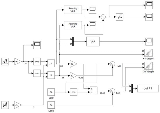
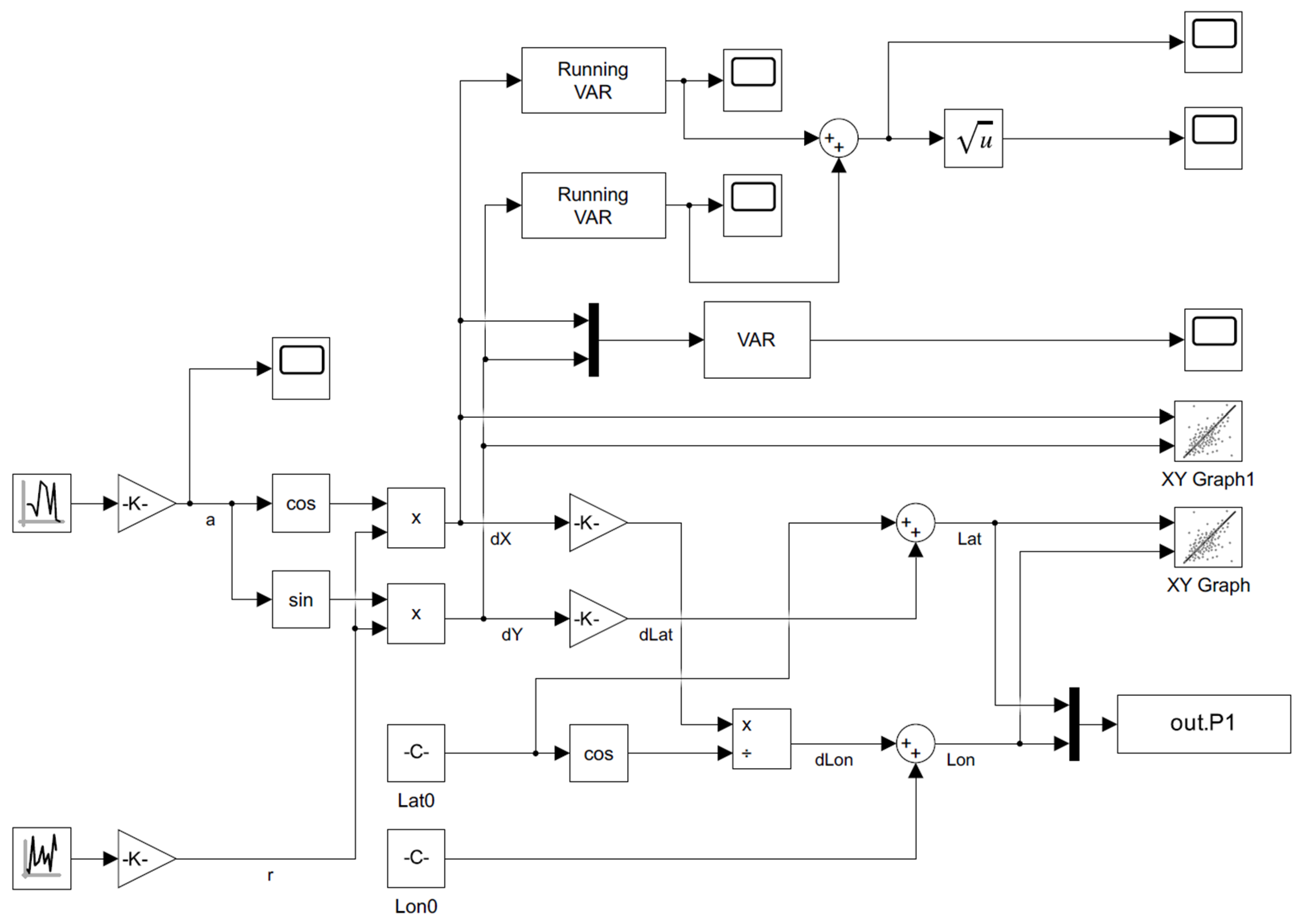
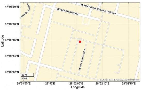
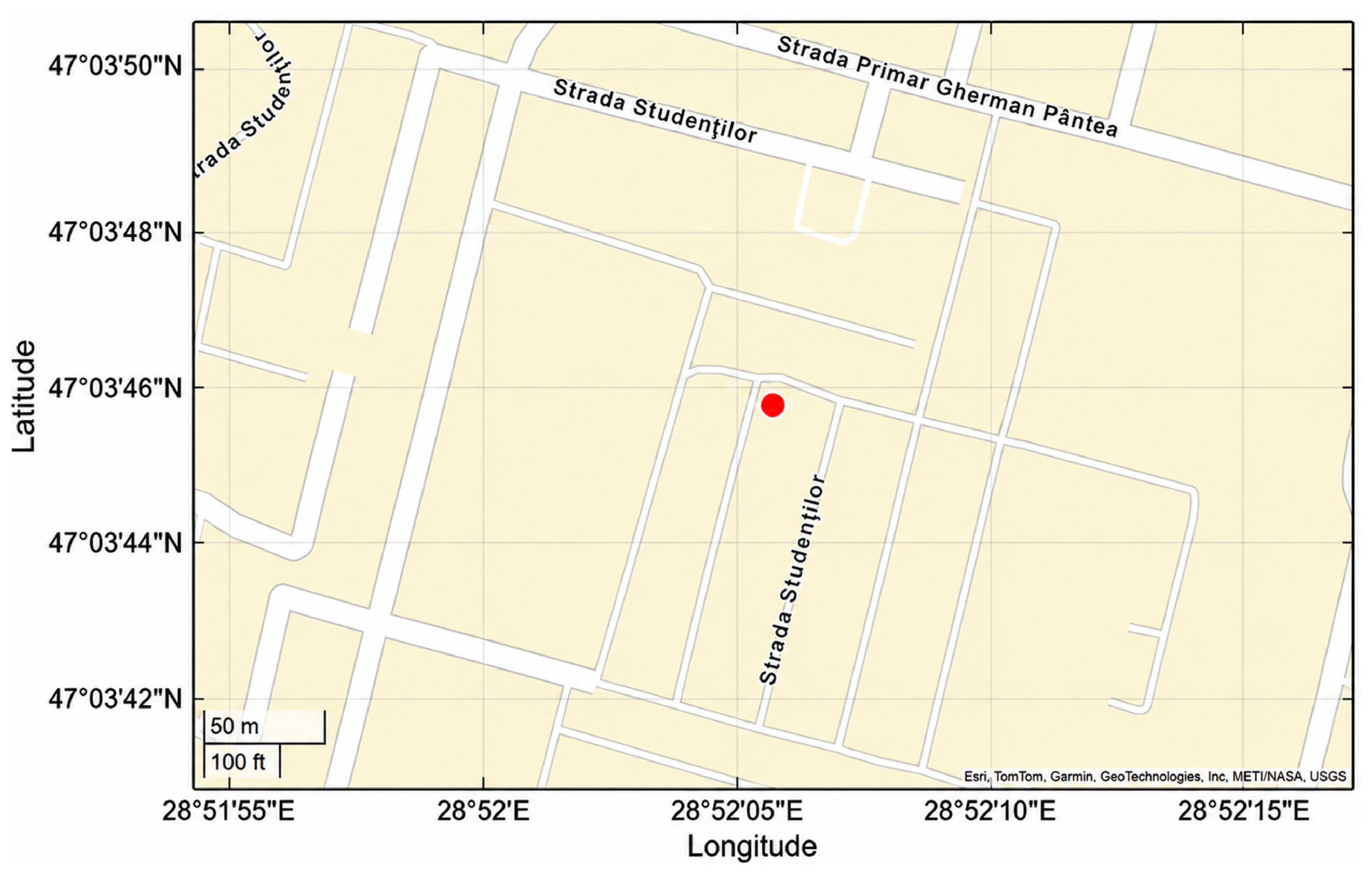
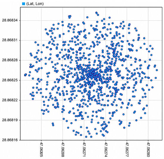
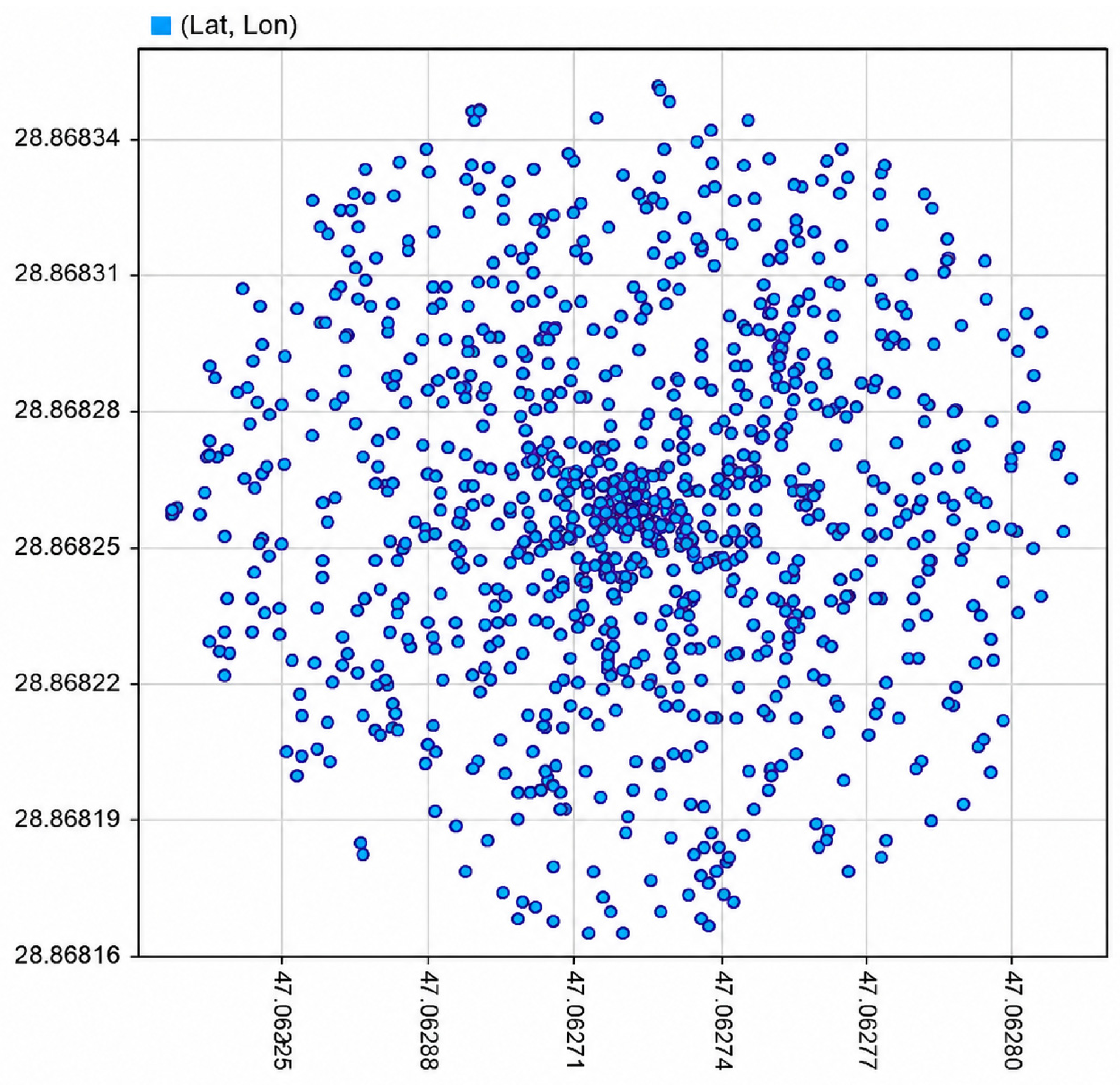
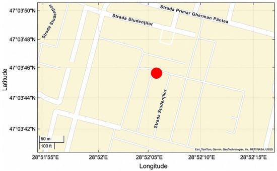
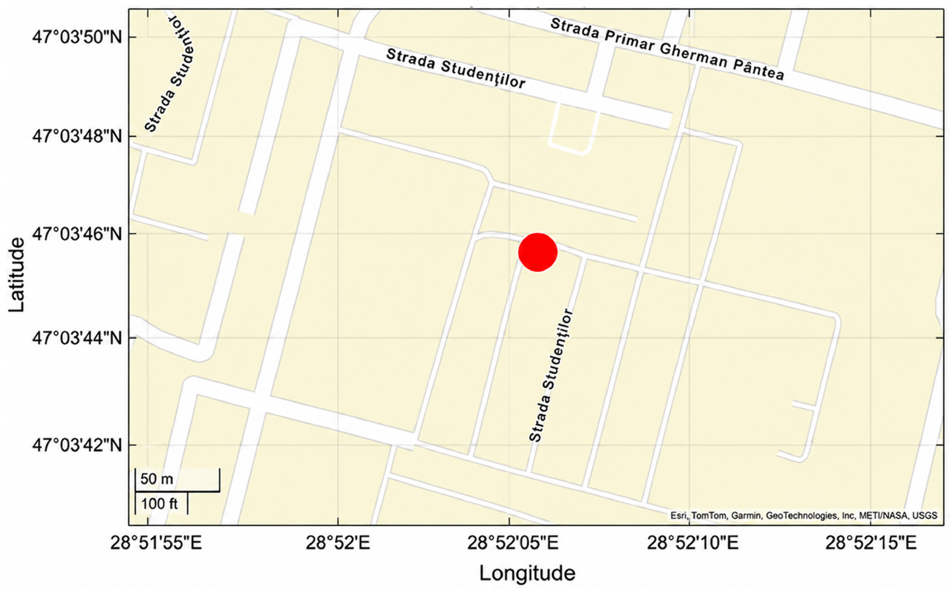
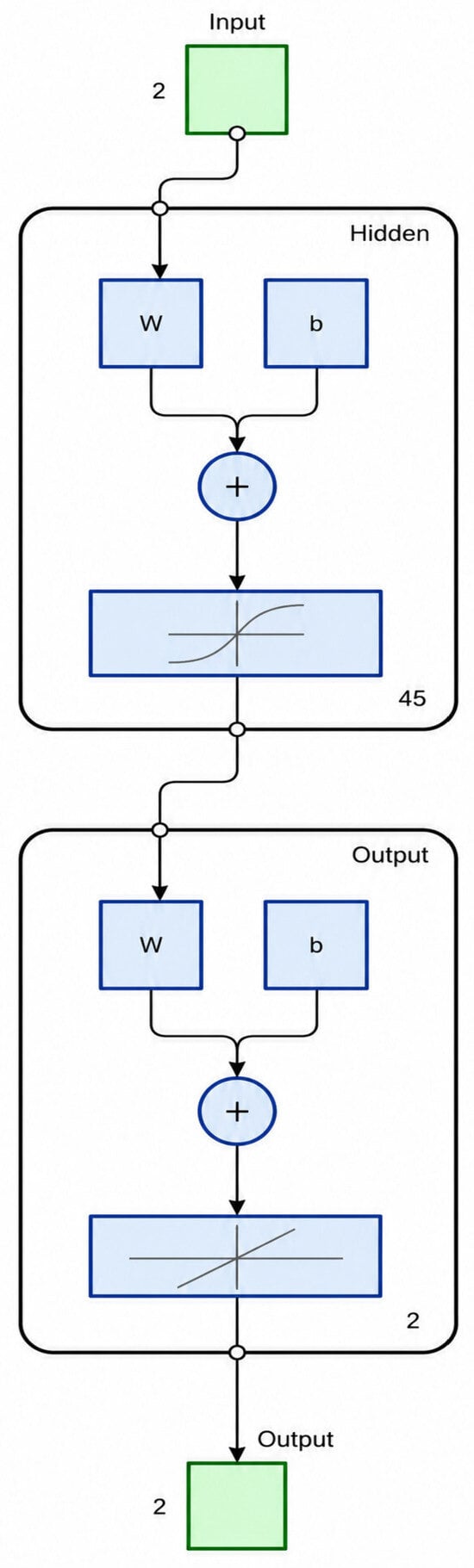
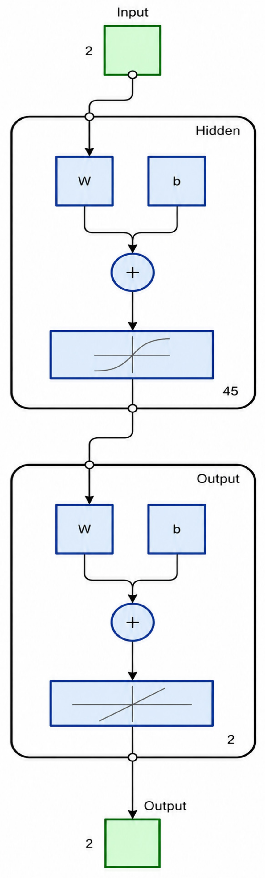
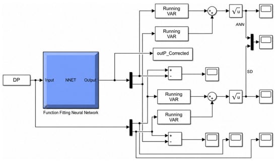
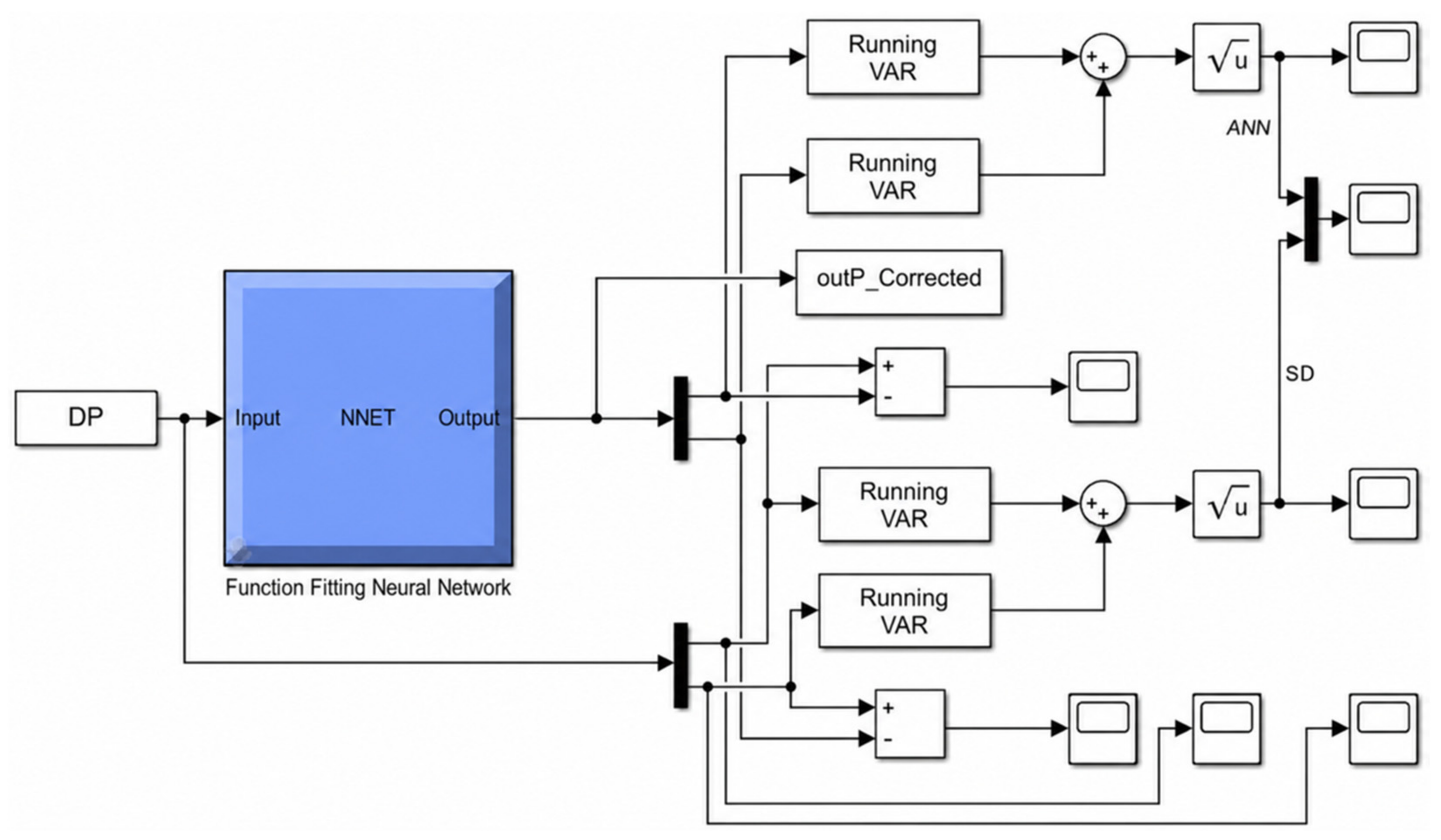
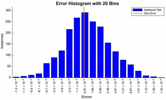
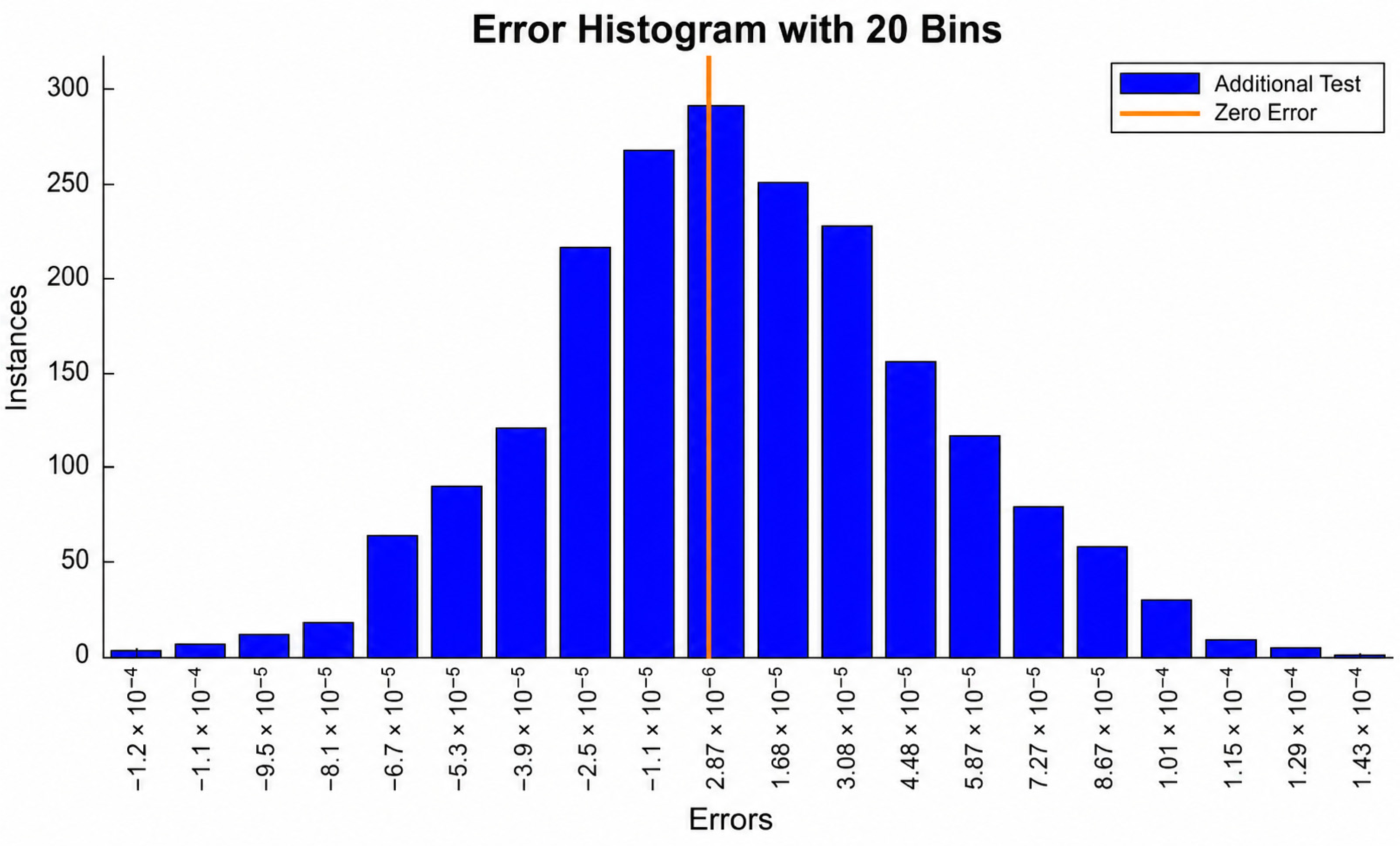
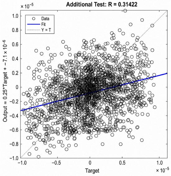
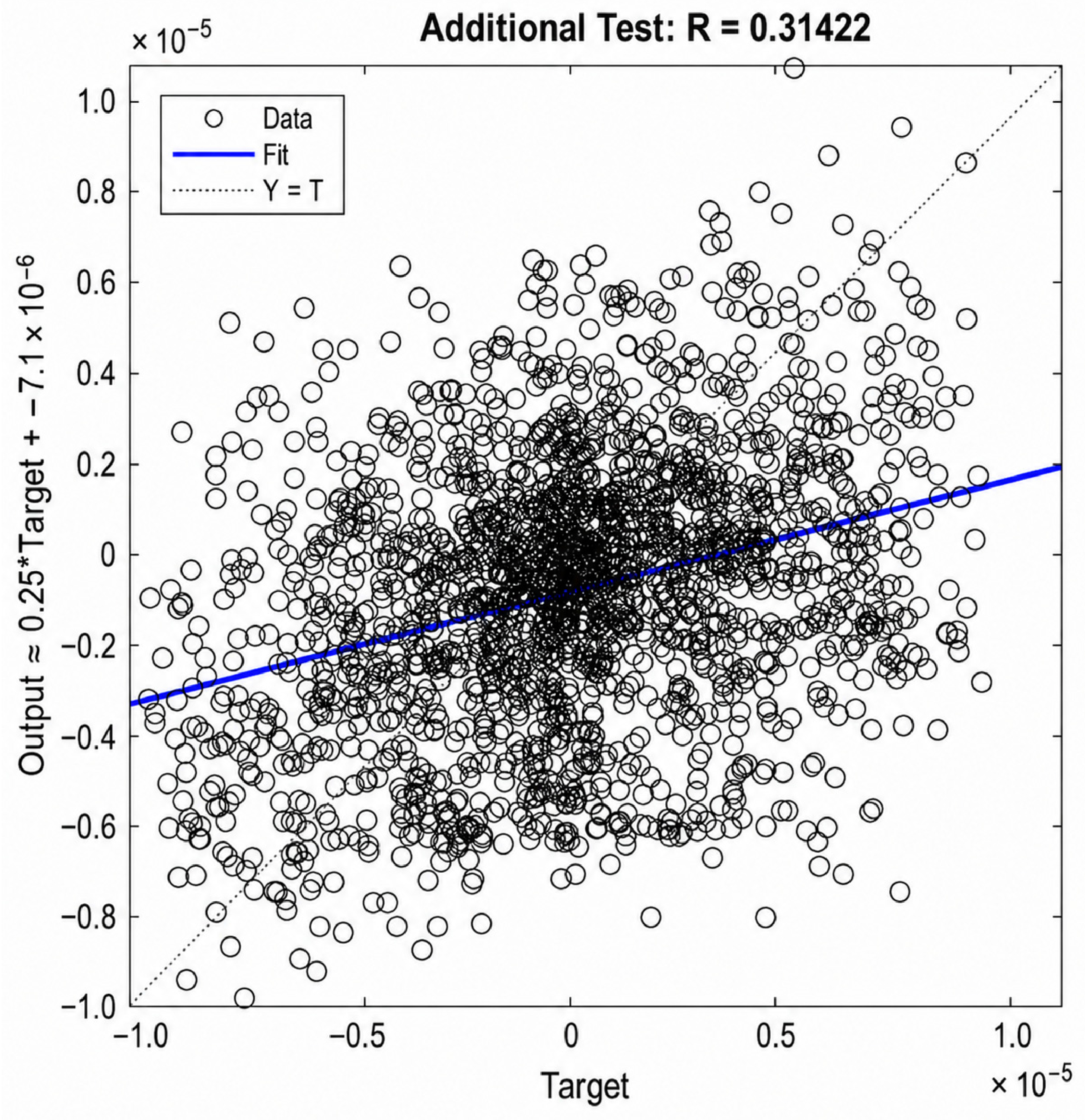
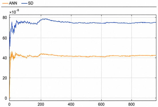
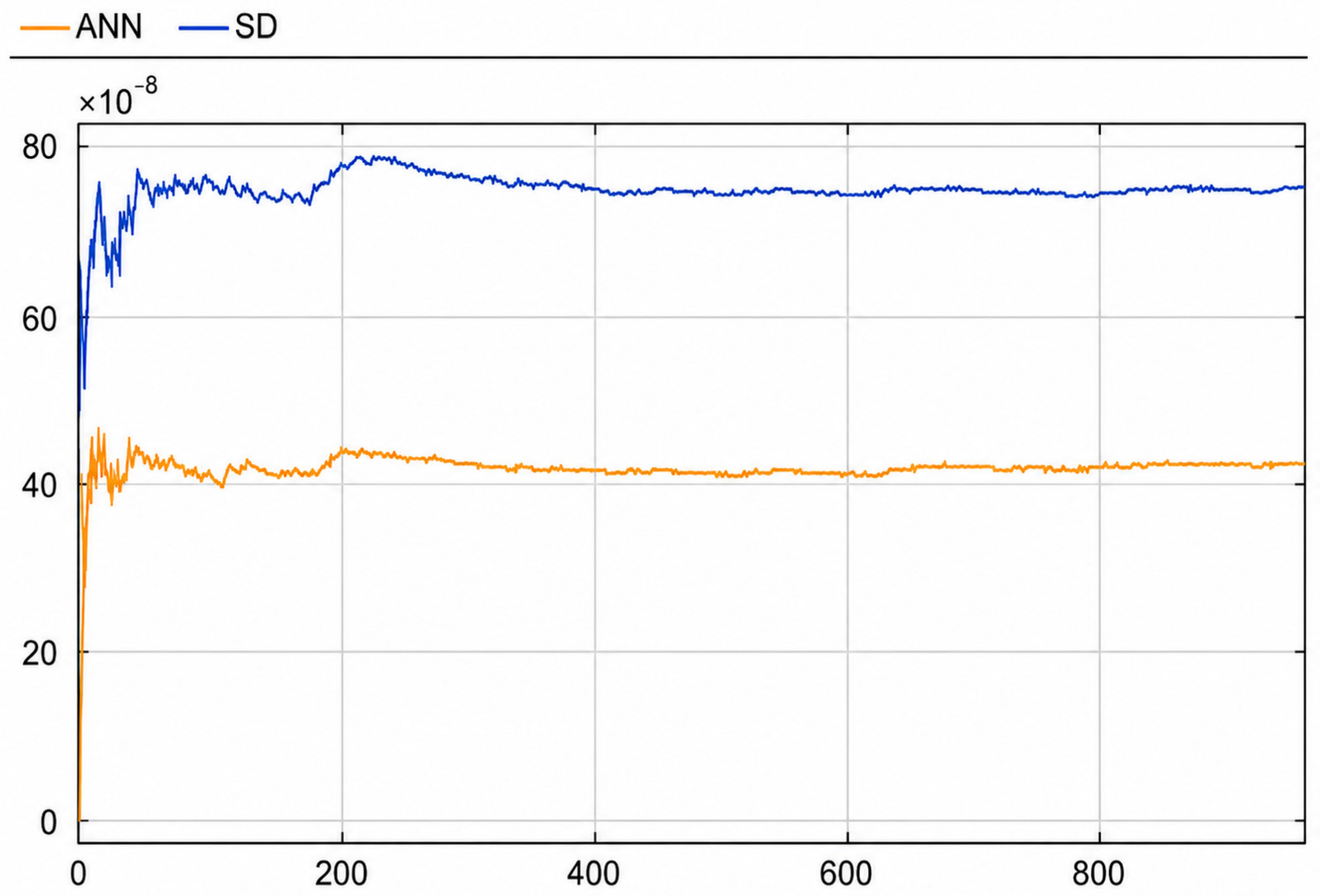
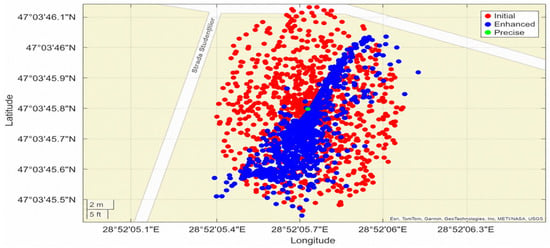
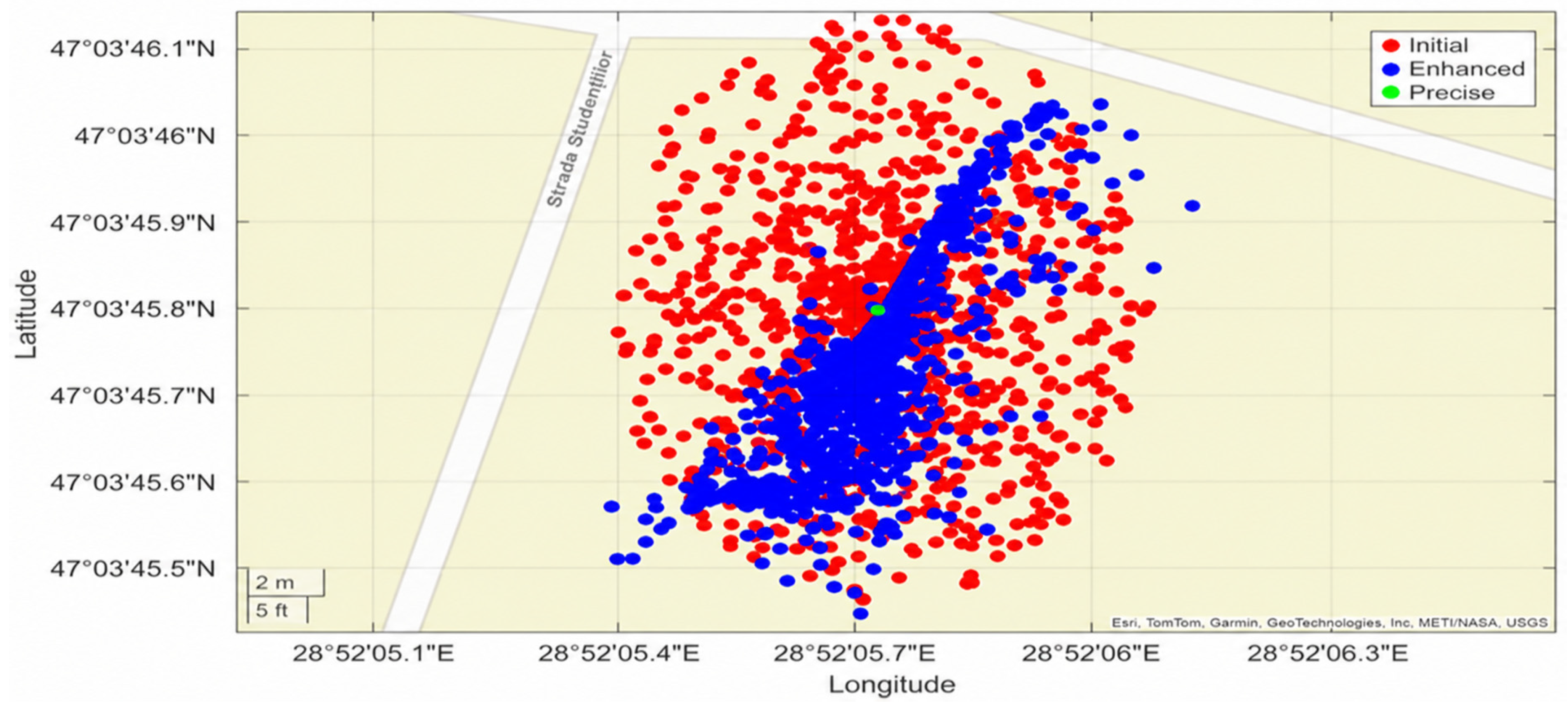
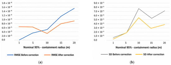

Disclaimer/Publisher’s Note: The statements, opinions and data contained in all publications are solely those of the individual author(s) and contributor(s) and not of MDPI and/or the editor(s). MDPI and/or the editor(s) disclaim responsibility for any injury to people or property resulting from any ideas, methods, instructions or products referred to in the content. |
© 2026 by the authors. Licensee MDPI, Basel, Switzerland. This article is an open access article distributed under the terms and conditions of the Creative Commons Attribution (CC BY) license.