


Abstract
The geosciences have witnessed a rapid expansion of analytical methods, from classical linear models to geostatistics and modern machine learning. However, no single resource compares a curated selection of these methods systematically while also providing reproducible code. This reproducibility-driven review evaluates seven analytical techniques applied to three simulated geoscience datasets: spatial points, time series, and a spatio-temporal grid. Methods were selected based on their availability in R to ensure transparency and accessibility. This paper serves as a historical review, a comparative benchmarking study, and a practical teaching resource with fully reproducible R code. The methods include linear regression, ARIMAX, ordinary kriging, regression-kriging, random forest, feed-forward neural networks, and BART. For spatial prediction, when evaluated against the true field, linear regression achieved the lowest mean RMSE (1.94 ± 0.23), followed by random forest (2.13 ± 0.23) and ordinary kriging (2.20 ± 0.26)—highlighting the importance of consistent out-of-sample validation. Regression-kriging performed similarly to ordinary kriging (2.22 ± 0.26). For time series, a feed-forward neural network (0.37 ± 0.09) substantially outperformed seasonal ARIMAX (1.90 ± 1.30). For spatio-temporal prediction, random forest and BART performed indistinguishably (0.534 ± 0.004 vs. 0.543 ± 0.004). A practical decision guide, grounded in these empirical results, summarises method selection based on sample size, data type, and research goal—whether inference, prediction, or uncertainty quantification. All code is open and reproducible, providing a template for future method comparisons.
1. Introduction
Over the past half-century, the geosciences have undergone a profound transformation in how data are analysed. Early studies relied heavily on classical statistical tools—linear regression, hypothesis testing, and basic time-series decomposition—applied to often sparse observations [1,2]. The digital revolution of the 1980s and 1990s brought geographic information systems (GISs) and geostatistics into routine use, allowing researchers to model spatial dependence quantitatively [3,4]. More recently, the explosive growth in computing power and data availability has pushed machine learning and deep learning to the forefront of geoscience research [5,6]. Today, a typical paper on hydrology, climatology, petrology, or mineral exploration might use random forests, convolutional neural networks, or gradient-boosted trees alongside traditional kriging or autoregressive models [7,8,9], with cutting-edge applications now successfully integrating physical constraints into modular deep learning architectures for complex tasks like simultaneous petrophysical property prediction [10].
This methodological layering is intellectually healthy, but it has created an unintended challenge to the research community: there is no single resource that traces the full evolution of analytical methods in the geosciences while also showing working scientists how to actually implement them. Existing reviews and textbooks fall into several categories, each with distinct limitations.
The first category comprises historical and narrative reviews. Classic works such as Matheron’s foundational 1963 paper introduced the principles of geostatistics to a broad audience [11], while Cressie’s 1989 review in The American Statistician articulated the many faces of spatial prediction [12]. More recently, Hengl et al. (2009), [13] performed a bibliometric analysis of the geostatistics literature, mapping the field’s intellectual structure. These historical accounts are invaluable for understanding where methods came from, but they were not designed as practical implementation guides. They rarely include code, and their data are often proprietary or no longer accessible.
The second category consists of comprehensive textbooks. Works like Webster and Oliver’s Geostatistics for Environmental Scientists (2nd ed., 2007) provide thorough coverage of variography, kriging, and spatial sampling [14]. Goovaerts’ Geostatistics for Natural Resources Evaluation (1997) remains a benchmark for theory-oriented readers [15]. Pebesma and Bivand’s (2005), [16] Computational Statistics introduced many geoscientists to the power of the R environment for spatial data analysis [16]. More practically oriented guides, such as Hengl’s A Practical Guide to Geostatistical Mapping (2009), explicitly combine R (“gstat”, “geoR”) with GIS workflows [17]. However, even textbooks with code examples are static documents that cannot be easily modified or re-run by the reader without significant manual effort.
The third category includes method-specific systematic reviews. For spatial interpolation alone, one can find dedicated reviews of kriging variants [18], inverse distance weighting [19], and spline methods [20]. For machine learning, numerous recent reviews focus narrowly on random forest applications in mineral prospectivity mapping [21,22], deep learning for remote sensing [23,24], or LSTM networks for hydrological forecasting [25]. Zhang et al. (2022) have provided a comprehensive review of machine learning, deep learning, and optimisation algorithms across geoengineering and geoscience [9]. Reichstein et al. (2019) have discussed deep learning as a tool for process understanding in Earth system science [6]. While each of these is excellent within its domain, none help a researcher compare a classical geostatistical method with a modern deep learning approach using the same data and the same evaluation metrics.
What is missing—and what this paper provides—is a reproducible methodological review that does three things together: (i) narrates the chronological evolution of analytical methods in the geosciences from the 1960s to the present; (ii) illustrates each major method with concise, working R code; and (iii) uses realistic simulated data throughout to ensure full reproducibility and to focus attention on the methods themselves rather than on data idiosyncrasies.
1.1. Why Simulated Data? A Justification
A critical reader might ask, “Why not use real-world case studies?” The answer is twofold. First, real geoscience data come with unavoidable idiosyncrasies—missing values, irregular spatial sampling, measurement error, and domain-specific conventions (such as compositional data in geochemistry or circular data in palaeomagnetism [26]). These complexities, while important in applied work, can obscure the core methodological comparison that a review paper aims to achieve. Second, and more fundamentally, reproducibility is the central scientific value of this paper. By providing the exact R code that generates every dataset and every figure, we allow any reader anywhere to re-run, modify, or extend our analyses without needing to negotiate access to proprietary data or to reconstruct undocumented pre-processing steps. This is particularly important for a review that intentionally spans multiple geoscience sub-disciplines. A hydrologist studying streamflow and a volcanologist modelling ash dispersion may not share the same field data, but both can understand and adapt a simulated spatial Gaussian field or a synthetic seasonal time series. The use of simulated data for methodological benchmarking is well established in the geostatistical literature (see, for example, the simulation exercises in [14,17]) and has been strongly advocated by proponents of reproducible research in the geosciences [27,28,29]. While real-world validation is a valuable extension, it is not a prerequisite for a methodological review whose primary contribution is a reproducible comparison framework and accessible R code. We emphasise that our simulated datasets are designed to be representative of common data structures, not exhaustive of all geoscience scenarios. The primary contribution is the reproducible framework, which can be adapted by readers to their own data.
1.2. What This Paper Is and Is Not
We do not claim to cover every analytical method ever used in the geosciences. Such an undertaking would be impractical if not impossible. Rather, we offer an integrated contribution that combines a chronological review of method evolution, a reproducible benchmarking exercise using simulated data, and a practical guide with working R code for readers to adapt to their own teaching or research. Instead, we focus on a curated set of representative methods that capture the major historical shifts in analytical thinking, with the understanding that many other valuable techniques (e.g., SVM, gradient boosting, GAMs, Gaussian processes, CNNs, and LSTMs) exist but are beyond the scope of a single reproducible review. It is acknowledged that requiring methods to have an R implementation introduces a selection bias; however, this is a deliberate choice to ensure full reproducibility and accessibility, which are the primary contributions of this work. The review is therefore reproducibility-driven rather than exhaustive or fully representative of all analytical developments in geoscience. This paper is structured around three distinct data types—spatial, temporal, and spatio-temporal—reflecting the diversity of geoscience problems. This integrated framework allows readers to see how different methods are suited to different data structures, and provides a practical guide for method selection. The three eras we identify are:
Era 1—Classical statistical methods (pre-1990s). This encompasses linear regression, trend decomposition, ARIMA modelling, and basic hypothesis testing. These methods remain the bedrock of much geoscience analysis, especially where interpretability and uncertainty quantification are paramount [2,30].
Era 2—Geostatistical and GIS-era methods (1990s–2010). This includes variogram modelling, ordinary and universal kriging, spatial interpolation, and raster-based terrain analysis. This era brought formal spatial dependence modelling into the mainstream of the geosciences [4,12,14,31].
Era 3—Machine learning and deep learning (2010–present). This covers random forests, gradient boosting, support vector machines, and recurrent neural networks (LSTMs). These methods excel at prediction with complex, high-dimensional data, although they often require careful attention to overfitting and interpretability [5,6,8,9].
For each era, we select two or three representative techniques, implement them in R on simulated data, discuss their strengths and weaknesses, and summarise their typical use cases in the geosciences. A decision guide (Section 5) helps readers navigate the trade-offs between predictive accuracy, interpretability, data requirements, and computational cost.
1.3. Intended Audience
This paper is written for three overlapping groups. The first is graduate students and early-career researchers who need a single entry point to understand how geoscience data analysis has evolved and, more practically, how to run a kriging or a random forest in R. The second is experienced geoscientists who are comfortable with one analytical paradigm (for example, geostatistics) but want to assess what newer machine learning methods can offer without wading through opaque code repositories or highly mathematical original papers. The third is methodologists, such as statisticians, engineers and computer scientists, working on geoscience applications—who may use this review as a benchmark for comparing new methods or as a teaching resource for interdisciplinary courses.
1.4. Roadmap
The remainder of this paper is organised as follows. Section 2 describes our systematic review methodology (search strategy, inclusion criteria, and data extraction protocol) and provides full details of the simulated data generation procedures. Section 3 presents the three eras in chronological order, with a summary table of key methods and their properties. Section 4 contains the core practical contribution: fully worked R examples for each selected method, including code, output figures, and brief interpretations. Section 5 provides a practical decision guide to help readers select an appropriate method for their own data and research questions. Section 6 outlines future directions, including physics-informed machine learning, causal inference from observational data, and the growing importance of fully reproducible workflows. Section 7 concludes with a call for more code-first, reproducible review papers across the geosciences. All code and simulated datasets are available in the Supplementary Material online. This paper is intentionally structured to cover three data types (spatial, temporal, and spatio-temporal), with each method demonstrated on the data type for which it is most appropriate. This integrated approach is a key contribution, not a limitation. Readers are strongly encouraged to run, modify, and adapt the code to their own teaching or research.
2. Methodology
2.1. Systematic Literature Review Protocol
To trace the evolution of analytical methods in the geosciences, we conducted a systematic literature review following a reproducible protocol informed by the PRISMA guidelines [32]. The search was performed across three bibliographic databases: Scopus (Elsevier), Web of Science Core Collection (Clarivate), and Google Scholar. The search period spanned from January 1960 to December 2023, capturing the emergence of modern geostatistics through the deep learning era. In addition to database searches, we manually examined the reference lists of key textbooks [4,14,15,33,34] and review papers [6,9,35] to identify seminal works that might not be indexed with our primary keywords.
Search keywords. Keywords were grouped by methodological era:
- -
- Classical statistics (1960–1990): “linear regression”, “multiple regression”, “time series analysis”, “ARIMA”, “trend decomposition”, “hypothesis testing”, combined with “geology”, “geophysics”, “hydrology”, “climatology”.
- -
- Geostatistics (1990–2010): “kriging”, “variogram”, “spatial interpolation”, “cokriging”, “simulation”, “geostatistics”, “spatial dependence”, combined with “Earth sciences”, “mineral exploration”, “soil science”.
- -
- Machine learning (2010–2023): “random forest”, “gradient boosting”, “support vector machine”, “neural network”, “deep learning”, “LSTM”, “convolutional neural network”, combined with “geoscience”, “remote sensing”, “geophysical inversion”.
The exact Boolean search strings used for each database are provided in the Supplementary Materials (Supplementary C).
Inclusion and exclusion criteria: A paper was included if: (a) it introduced or significantly advanced a quantitative method applicable to geoscience data; (b) the method was either historically seminal (e.g., Matheron 1963 [10]) or widely cited (>100 citations in Scopus for pre-2015 papers, >50 citations for post-2015 papers); and (c) the method could be implemented in R using publicly available packages (e.g., “gstat” [36], “randomForest”, “keras”). A paper was excluded if: (a) it was purely theoretical without any geoscience example or simulation; (b) it required proprietary software (e.g., ArcGIS only, without an R alternative); or (c) it was not available in English.
Screening and final corpus: The initial search returned 347 unique records after duplicate removal. Two rounds of title and abstract screening reduced the corpus to 112 potentially relevant papers. Full-text examination yielded 77 references that met our inclusion criteria. Figure 1 presents the PRISMA flow diagram of the search and selection process, showing the final included corpus of 77 references. Beyond counting publications, our analysis of the selected literature reveals several recurring themes: the persistent tension between interpretability and predictive accuracy, the growing importance of uncertainty quantification, and the increasing reliance on open-source software for reproducible research. We also note that while machine learning methods have gained prominence, classical and geostatistical approaches remain essential, particularly where data are sparse or where physical interpretability is required. These tensions form the basis for the critical synthesis presented in Section 3.
Figure 1.
PRISMA flow diagram of the systematic literature search and screening process.
To provide a more structured synthesis, we categorised the 77 reviewed studies into three thematic groups: (i) studies that compare multiple methods on the same dataset (approximately 30% of the corpus); (ii) studies that introduce or extend a single method (approximately 50%); and (iii) review papers that synthesise methodological trends without new implementations (approximately 20%). Across all three groups, we identified several recurring limitations: limited uncertainty quantification, lack of reproducible code, and narrow scope (focused on a single data type). These gaps motivated our integrated, reproducibility-driven framework, which covers spatial, temporal, and spatio-temporal data with fully open code.
Figure 1 presents the PRISMA flow diagram of the search and selection process.
2.2. Simulated Data Generation
To enable a transparent, reproducible comparison of methods across eras, we designed three synthetic datasets that mimic common data structures in geoscience research. All datasets include clearly defined independent variables (predictors, coordinates, or time) and dependent variables (responses). This ensures that readers can evaluate how each method handles relationships between predictors and outcomes, including linear, non-linear, and spatio-temporal dependencies.
Why simulated data? Real-world geoscience data inevitably contain missing values, irregular sampling, measurement errors, and domain-specific complexities (e.g., compositional closure, circular data [26,37]). While these are important in applied work, they obscure methodological comparison. Simulated data with known ground truth allow us to quantify each method’s accuracy (e.g., prediction error relative to the true field) and to isolate the effects of sample size, noise level, and spatial/temporal structure. Furthermore, simulated data ensure full reproducibility: any reader can run our code and obtain identical results without seeking data permissions.
All simulations were performed in R version 4.5.1 [38] with the following packages: “sp” [39] for spatial data classes, “gstat” [36,40,41,42] for variogram modelling and kriging simulation, “lhs” [43] for Latin hypercube sampling, “ggplot2” [39] for visualisation, and “dplyr” [32] for data manipulation. The random seed was set to “20250511” for all stochastic operations, ensuring exact reproducibility. To assess robustness, the full analysis was repeated across 10 different random seeds (1–10). The results reported in Section 4 are the mean RMSE (± standard deviation) across these seeds. For clarity, we assign nominal physical units to the simulated domains: spatial coordinates are in metres (m), and time steps are in days. These units are illustrative and can be adapted to any real-world context. The complete R code is provided in the Supplementary Material online. Dataset 1 uses spatial point data. This dataset mimics a regionalised variable such as soil contaminant concentration, ore grade, or temperature measured at point locations. Table 1 summarises its structure. Dataset 2 presents time series data. This dataset resembles a hydrological or climatic variable (e.g., streamflow, temperature) with trend, seasonality, and autoregressive errors. Table 2 summarises its structure. A spatio-temporal grid is simulated in Dataset 3. This dataset mimics a moving geophysical anomaly (e.g., atmospheric front, contaminant plume, seismic wavefield). Table 3 summarises its structure.
Table 1.
Parameters of the simulated spatial point dataset (Dataset 1).
Table 2.
Parameters of the simulated time series dataset (Dataset 2).
Table 3.
Parameters of the simulated spatio-temporal grid dataset (Dataset 3).
2.3. Selected Methods for Demonstration
From the three eras described in Section 3, we selected two/three representative methods per era for detailed implementation in R (Section 4). Selection criteria were: (i) historical importance, (ii) current usage frequency in the geoscience literature (based on our search results), (iii) availability of stable, well-documented R packages, and (iv) complementarity (e.g., one parametric and one non-parametric or one interpretable and one prediction-focused). Table 4 lists the selected methods.
Table 4.
Methods selected for detailed R demonstration, grouped by era.
For each method, Section 4 provides: (a) a brief conceptual description, (b) the complete R code used to fit the model to the relevant simulated dataset, (c) output figures (predictions vs. actuals, residuals, accuracy metrics such as RMSE and R2), and (d) a short discussion of strengths, limitations, and computational cost.
2.4. Reproducibility and Quality Assurance
To meet the standards of journal publication and to ensure that this review serves as a reliable resource, we implemented the following measures:
- Fixed random seed: set.seed(20250511) ensures all stochastic simulations (Latin hypercube, Gaussian fields, ARIMA errors) are deterministic [44,45].
- Version control: The code was tested on a clean R installation version 4.5.1 (no user-specific libraries) to confirm portability.
- Literate programming: The manuscript was written as an R Markdown document, interleaving text and code. Every number reported in the results (e.g., variogram parameters, RMSE values) is computed dynamically from the code, eliminating manual transcription errors.
- Data and code availability statement: Included at the end of the manuscript, before the references.
Figure 2 summarises a tabular comparison of the seven methods across five criteria: interpretability, predictive accuracy, data requirements, computational cost, and handling of non-linearity. Figure 3 presents a decision tree to help readers select an appropriate method based on their research question (e.g., prediction vs. inference), sample size, and presence of spatial/temporal dependence. These conceptual figures are described in the captions; their design follows standard flowchart conventions.
Figure 2.
Comparison of seven analytical methods across five evaluation criteria. Methods: LM = linear regression, OK = ordinary kriging, RK = regression-kriging, RF = random forest, NN = neural network, BART = Bayesian additive regression trees. Symbols: ++ excellent, + good, 0 moderate, – poor, N/A not applicable.
Figure 3.
Decision tree for selecting an appropriate method based on research goal and data characteristics. Solid lines indicate primary pathways; dashed/dotted lines indicate alternative options. Method abbreviations: RF = random forest, OK = ordinary kriging, RK = regression-kriging, LM = linear regression, NN = neural network, BART = Bayesian additive regression trees.
2.5. Summary
This section has detailed: (i) the systematic literature search protocol (Section 2.1), (ii) the design and justification of three realistic simulated datasets with clear dependent and independent variables, summarised in Table 1, Table 2 and Table 3 (Section 2.2), (iii) the selection of six representative methods across three eras (Table 4, Section 2.3), and (iv) the reproducibility measures that underpin this review (Section 2.4). All code and data are publicly available. The next section (Section 3) presents the chronological evolution of these methods, from classical statistics through geostatistics to modern machine learning.
3. Three Eras of Analytical Methods in the Geosciences
The history of quantitative methods in the geosciences can be divided into three broad eras, each defined by a dominant analytical paradigm. These eras overlap in time and continue to coexist today. The first era, classical statistics, focused on linear models, hypothesis testing, and time series decomposition. The second era brought geostatistics and spatial thinking into the mainstream, formalising the analysis of spatially dependent data. The third era, driven by computational advances, introduced machine learning and deep learning, enabling predictions from high-dimensional and non-linear systems. This section traces the evolution of methods within each era, highlighting key innovations and their lasting impact on geoscience practice.
3.1. Era 1—Classical Statistical Methods (Pre-1990s)
Before the widespread adoption of geostatistics, most geoscience data analysis relied on tools from classical statistics. Linear regression, analysis of variance, and basic time series methods formed the core of quantitative reasoning in geology, geophysics, and hydrology [1,2]. These methods assume independence of observations or simple temporal dependence structures, which was often reasonable for sparse, well-designed surveys or for data collected along boreholes or time series.
Multiple linear regression became the workhorse for exploring relationships between geological variables. For example, early petrological studies used regression to relate mineral composition to bulk rock chemistry [1]. In hydrogeology, regression models linked well yield to aquifer properties. The appeal of regression lay in its interpretability: coefficients directly quantified the effect of each predictor. However, regression assumes uncorrelated errors, a condition frequently violated in spatial or temporal data [12]. The work of Box and Jenkins [46] revolutionised how geoscientists analysed temporal data. ARIMA (Autoregressive Integrated Moving Average) models provided a systematic way to handle trend, seasonality, and autocorrelation. In hydrology, ARIMA models were applied to streamflow forecasting [2]; in geophysics, they helped characterise seismic noise. Despite their power, classical time series methods do not naturally extend to spatial data or to non-stationary spatial processes.
The main shortcoming was the neglect of spatial dependence. Geoscience data are almost always spatially correlated, and ignoring this correlation leads to biased standard errors, overconfident predictions, and inefficient use of information [33]. The classical era also lacked computational power for iterative methods, so linearity and normality were often assumed for mathematical convenience. We acknowledge that each of these classical methods has spawned numerous extensions (e.g., SARIMAX, NARIMAX, and ARIMA-GARCH), but our focus here is on the foundational paradigm shifts rather than an exhaustive treatment of every variant.
3.2. Era 2—Geostatistics and GIS-Era Methods (1990s–2010)
The second era was defined by two parallel developments: the formalisation of geostatistics and the proliferation of geographic information systems (GISs). Geostatistics provided a rigorous framework for modelling spatial dependence and making optimal predictions at unsampled locations [4,11,12]. GISs made it possible to manage, visualise, and analyse large spatial datasets, bringing spatial thinking to every geoscience discipline.
The core innovation of geostatistics was the variogram, a function that quantifies how spatial correlation decays with distance [4,31]. By fitting a variogram model (spherical, exponential, or Gaussian), a geoscientist could describe the spatial structure of a variable. Ordinary kriging then uses this variogram to compute best linear unbiased predictions at unsampled locations, complete with a prediction variance [12]. Kriging became standard in mineral resource estimation, soil mapping, and environmental monitoring [14,15]. To handle regional trends, geostatisticians developed universal kriging and regression-kriging [47]. These methods combine a deterministic trend (modelled by regression) with a kriged residual. This hybrid approach remains popular because it captures both large-scale patterns and local spatial detail.
The rise of GISs allowed geoscientists to integrate multiple data layers—geology, geochemistry, and geophysics—within a single coordinate system [3,35,48,49,50,51,52]. Early GISs were raster-based, enabling map algebra and terrain analysis. Later, vector-based GISs supported sophisticated spatial queries and neighbourhood operations. GISs did not replace geostatistics but complemented it; many geostatistical analyses were performed within or alongside GIS environments [17,53,54]. Kriging assumes second-order stationarity (constant mean and variance across the domain) or intrinsic stationarity. Real datasets often violate these assumptions. Moreover, kriging becomes computationally expensive for large datasets (n > 10,000) because it requires solving systems of equations of size n. Multivariate extensions such as cokriging are even more demanding. Finally, kriging is essentially a linear predictor; it cannot capture non-linear relationships without transformation.
3.3. Era 3—Machine Learning and Deep Learning (2010–Present)
The third era began around 2010, driven by three factors: the exponential growth of geoscience data (satellite imagery, sensor networks, and seismic arrays), the availability of powerful computing hardware (GPUs, cloud computing), and methodological advances in statistics and computer science [5,6,7]. Machine learning methods excel at prediction from high-dimensional, non-linear, and non-stationary data. They have been applied to mineral prospectivity mapping, landslide susceptibility, earthquake detection, climate downscaling, and many other problems [8,9].
Ensemble methods, particularly random forest [55,56,57] and gradient boosting [58] (e.g., XGBoost), have become ubiquitous in the geosciences. Random forest builds many decision trees on bootstrapped samples and averages their predictions. It handles mixed data types (continuous and categorical), automatically captures interactions and non-linearities, and provides variable importance measures. In mineral exploration, random forest has outperformed traditional weights-of-evidence and logistic regression [21,22]. In hydrology, random forest has been used for rainfall-runoff modelling and groundwater level prediction, and the quantification of post-rainfall moisture content in pavement unbound layers using long-term performance data [59,60]. Support vector machines (SVMs) were popular in the 2000s for classification problems such as lithology identification from well logs. However, SVMs scale poorly to large datasets. Neural networks, after decades of dormancy, returned with deep learning architectures. Convolutional neural networks (CNNs) are now standard for satellite image classification, seismic facies analysis, and geological mapping [23,24].
Feed-forward neural networks with lagged inputs provide a flexible non-linear alternative to classical time series models. A single hidden layer network can approximate any continuous function and capture non-linear dependencies in sequential data [61,62]. For hydrological forecasting, such networks have been shown to outperform linear models when sufficient training data are available. More complex recurrent architectures, such as long short-term memory (LSTM) networks, have also been successfully applied to rainfall-runoff prediction [25,46] and other geoscience time series, but they require substantial computational resources and are beyond the scope of this reproducible review. While we discuss LSTMs and gradient boosting as part of the broader historical evolution of machine learning in the geosciences, our implementation focuses on random forest and a simple feed-forward neural network due to their accessibility, ease of implementation in R, and suitability for a reproducible teaching-oriented review.
In this study, we therefore implement a single-hidden-layer feed-forward neural network (using the nnet package in R) to forecast the simulated time series, using ten past observations as inputs. BART is a Bayesian non-parametric ensemble method that combines sum-of-trees models with regularisation priors [57]. Unlike random forest, which produces point predictions, BART provides full posterior distributions for predictions, naturally quantifying prediction uncertainty. BART has been successfully applied in ecological modelling [63], noise pollution prediction [64], and probabilistic wind speed forecasting [65,66]. In this study, we apply BART to the spatio-temporal grid (Dataset 3) as a second machine learning benchmark, implemented via the BART package in R.
Machine learning methods are data-driven, flexible, and often achieve higher predictive accuracy than classical or geostatistical methods, especially when the underlying processes are complex or poorly understood. They do not require strong assumptions about stationarity or linearity. Feature engineering, once a bottleneck, has been partially automated by deep learning. It should be noted that machine learning methods are not a panacea. They typically require large training datasets (hundreds to thousands of labelled examples)—a condition not always met in geoscience. They are often black boxes, offering little insight into the underlying physical processes. Overfitting is a constant danger, and careful validation (cross-validation and separate test sets) is essential. Moreover, geoscience data are often imbalanced (few rare events), spatially correlated, or contain measurement errors that violate the independence assumptions of standard ML algorithms. Recent work on physics-informed machine learning attempts to embed domain knowledge into neural networks, improving generalisation and interpretability [6].
3.4. Summary of the Three Eras
Table 5 summarises the key characteristics of each era. Classical methods remain valuable for small datasets, simple problems, and when interpretability is paramount. Geostatistical methods are still the gold standard for spatial interpolation when stationarity holds, and computational resources are modest. Machine learning methods are increasingly the first choice for large, complex, prediction-oriented problems, provided that enough training data exist and that the user attends carefully to validation and overfitting. The methods from all three eras continue to be used, often in combination—for example, regression-kriging with a random forest trend, or LSTM residuals after removing a seasonal component. The thematic synthesis presented in Section 2.1 underpins the following summary of the three eras, connecting the literature gaps to the methodological trends discussed below.
Table 5.
Synthesis of the three methodological eras in the geosciences, highlighting not only their strengths but also their inherent limitations and the circumstances under which each remains the method of choice. This synthesis draws on the literature reviewed in Section 2.1 and Section 3.1, Section 3.2 and Section 3.3.
4. Results
4.1. Overview of Simulated Datasets
Before applying any modelling method, we visualised the three simulated datasets to confirm their structure. Figure 4 presents panel plots for each dataset. For Dataset 1 (spatial points, panels a–d), the sample locations cover the domain evenly, the observed Z values show a clear north-south gradient, the experimental variogram exhibits a spherical shape consistent with the true model (nugget ~0.5, partial sill ~2.0, range ~30), and the true field (panel d) illustrates the underlying spatial structure. For Dataset 2 (time series, panels e–h), the series Y(t) displays a positive trend and annual seasonality, the ACF decays slowly (indicating non-stationarity), the PACF cuts off after lag 1, and the STL decomposition extracts a smooth trend component. For Dataset 3 (spatio-temporal grid, panels i–k), the spatial slice at t = 1 shows a stationary pulse centred at (5,5), the slice at t = 25 captures the pulse shifted to approximately (10,7.5), and the time series at pixel (10,10) records the passage of the pulse with superimposed noise. These diagnostics confirm that the simulated data match the intended design described in Section 2.
Figure 4.
Visualisation of the three simulated datasets. Panels (a–d): Spatial dataset (Dataset 1)—(a) sample locations, (b) observed Z values, (c) experimental variogram, (d) true field. Panels (e–h): Time series dataset (Dataset 2)—(e) Y(t) over time, (f) autocorrelation function, (g) partial autocorrelation function, (h) trend component from STL decomposition. Panels (i–k): Spatio-temporal grid (Dataset 3)—(i) spatial slice at t = 1, (j) spatial slice at t = 25, (k) time series at pixel (10,10).
4.2. Classical Statistical Methods
4.2.1. Linear Regression (Dataset 1)
Multiple linear regression was fitted to the spatial points with Z as the response and x and y as predictors. The fitted model was:
All coefficients were statistically significant (p < 0.01). The adjusted R2 was 0.237, and when evaluated against the true simulated field, the RMSE was 1.91. Residual plots (Supplementary Materials, Figure S1) show that residuals are approximately homoscedastic but retain spatial correlation, indicating that a pure linear trend is insufficient to capture the spatial dependence.
4.2.2. ARIMAX Modelling (Dataset 2)
Because the simulated time series includes known exogenous variables (trend X1, seasonality X2, and noise X3), we fitted a regression model with ARIMA errors. The “auto.arima” procedure selected an ARIMA (2,0,0) model with exogenous regressors. The fitted coefficients for X1, X2, and X3 were −1.12, 1.21 and 0.32, respectively, with all standard errors small. The model was trained on the first 400 observations and used to forecast the next 20 time steps. The test RMSE was 1.437. Of the 500 simulated observations, the first 400 were used for training, the following 20 for the reported forecast evaluation, and the remaining 80 are unused in this analysis but available for readers to extend the test horizon. Figure S2 (Supplementary Materials) compares the forecast with the observed test values, and Figure S3 shows the full series with the forecast extension. The residuals from the ARIMAX model (ACF and histogram in Figures S4 and S5) appear approximately white noise, indicating an adequate fit.
4.3. Geostatistical Methods (Dataset 1)
4.3.1. Variogram Modelling
The experimental variogram of Z was computed and fitted with a spherical model as shown in Figure 5. The fitted parameters were nugget = 0.50, partial sill = 3.52, and range = 47.8. While the nugget matched the true value (0.5), the partial sill was higher (true = 2.0) and the range longer (true = 30), reflecting the particular realisation of the random field.
Figure 5.
Experimental and fitted spherical variogram for Dataset 1. Black dots represent the experimental semivariances calculated from the sample data; the red line shows the fitted spherical variogram model.
4.3.2. Ordinary Kriging (OK)
Ordinary kriging was applied to predict Z on a 50 × 50 grid [66]. When evaluated against the true simulated field Figure 6 (panel C), ordinary kriging gave an RMSE of 2.45. Figure 6 presents four panels: (A) the ordinary kriging prediction map, which captures the large-scale spatial gradient; (B) the kriging variance map, showing higher uncertainty near the domain boundaries and in data-sparse regions; (C) the true simulated field (from the unconditional simulation used in Code S1), provided for visual reference; and (D) the regression-kriging prediction map discussed below.
Figure 6.
Geostatistical predictions and reference field. (A) Ordinary kriging prediction, (B) kriging variance, (C) true simulated field, (D) regression-kriging prediction.
4.3.3. Regression-Kriging (RK)
Regression-kriging combined the linear trend (Section 4.2.1) with kriging of the residuals. The residual variogram was fitted, and the RK predictions are shown in Figure 6 (panel D). The RMSE of RK against the true simulated field (panel C) was 2.45. When ordinary kriging was evaluated against the same true field, it also gave 2.45, indicating that the two methods performed similarly under a consistent evaluation framework. The earlier apparent underperformance of RK was an artefact of inconsistent validation (RK vs. true field, OK vs. cross-validation), not a failure of the method itself. We return to this in Section 5.
4.4. Machine Learning Methods
4.4.1. Random Forest for Spatial Prediction (Dataset 1)
A random forest with 500 trees was trained to predict Z from x and y. The model explained 60.7% of the variance, with a training RMSE of 0.590. Variable importance indicated that x contributed more than y (%IncMSE = 73.7 vs. 48.8). Figure 7 (left panel a) shows predicted vs. observed values, with points clustering closely around the 1:1 line, confirming the excellent fit. When evaluated against the true simulated field (Figure 6 (panel c)), random forest gave an RMSE of 2.22. While this is higher than its training error (0.59), it is comparable to ordinary kriging (2.45) and suggests overfitting of the sample points, a point we discuss in Section 5.
Figure 7.
Machine learning results: (a) Random Forest predicted vs. observed (Dataset 1). Black dots represent individual predictions; the red dashed line indicates the 1:1 reference line (perfect agreement between observed and predicted values). (b) neural network forecast 20 steps ahead (Dataset 2).
4.4.2. Feed-Forward Neural Network for Time Series (Dataset 2)
A single-hidden-layer neural network (10 hidden units) was trained to forecast Y(t) using ten lagged values as inputs. The network architecture consists of a single hidden layer with 10 units, linear output activation, and was trained using the nnet package with 200 iterations. The small network size and use of a separate test set (last 20 observations) help mitigate overfitting risk. We acknowledge that the neural network and ARIMAX models have different input structures (lagged values vs. autoregressive and exogenous terms), reflecting their different underlying paradigms. The comparison is intended to illustrate the relative strengths and weaknesses of each approach for the same forecasting task, not to assert superiority of one over the other. We acknowledge that a more controlled comparison using equivalent predictor information (e.g., ARIMA vs. lag-only neural network or ARIMAX vs. neural network with exogenous inputs) would be valuable; however, our comparison reflects the standard implementation of each method in practice. Training used the first 400 observations; the next 20 were held out for testing. The test RMSE was 0.447, substantially lower than the ARIMAX test RMSE (1.437). Figure 7 (right panel (b)) displays the neural network forecast alongside the observed test series. The forecast tracks the test data closely, with narrow deviations. Residual diagnostics indicated no severe autocorrelation. This demonstrates that a simple neural network can outperform a classical seasonal ARIMAX model for this dataset.
4.4.3. Spatio-Temporal Predictions (Dataset 3)
We applied two machine learning methods to predict at time steps 41–50 using the ten previous time steps and spatial coordinates as predictors. Training used time steps 11–40 (after accounting for lags).
Random forest achieved a test RMSE of 0.534 ± 0.004. BART produced a test RMSE of 0.543 ± 0.004. These values are indistinguishable within the variability across seeds, indicating that the two methods performed equivalently on this dataset. Figure 8 shows observed vs. predicted scatter plots for both methods; points lie reasonably close to the 1:1 line, though with some scatter reflecting the noise level (σ = 0.5). Figure 9 illustrates the time series for four randomly selected cells, comparing observed values with random forest and BART predictions. Both methods capture the main pulse dynamics, with BART providing slightly smoother predictions (not visible in RMSE). The indistinguishable performance suggests that for this dataset, the additional complexity of BART does not improve accuracy over random forest.
Figure 8.
Observed vs. predicted for spatio-temporal test set: left—random forest, right—BART. Black dots represent individual predictions; the red dashed line indicates the 1:1 reference line (perfect agreement between observed and predicted values). Section 4.4.3.
Figure 9.
Time series of observed, random forest, and BART predictions for four randomly selected grid cells (test period). Section 4.4.3.
4.5. Summary of Method Performance
Table 6 summarises the mean RMSE (± standard deviation) for all methods across 10 simulation seeds. For Dataset 1 (spatial), when all methods were evaluated against the true field, linear regression gave the lowest RMSE (1.91), followed by random forest (2.22), ordinary kriging (2.45), and regression-kriging (2.45). This ranking differs from the training-based comparison, underscoring the importance of consistent validation. For Dataset 2 (time series), the neural network (nnet) achieved a lower test RMSE than the ARIMAX model on this specific dataset, though the comparison is illustrative rather than definitive, given the different input structures. For Dataset 3 (spatio-temporal), random forest and BART performed indistinguishably (0.534 ± 0.004 vs. 0.543 ± 0.004). Geostatistical methods performed similarly; ordinary kriging and regression-kriging both achieved RMSE 2.45 when evaluated against the true field. These differences are discussed further in Section 5. We acknowledge that alternative performance metrics (e.g., bias, prediction interval coverage, and computational time) could provide additional insights; our reproducible code framework enables readers to easily compute these metrics for their own applications.
Table 6.
Prediction RMSE for all methods. Values for Dataset 1 are evaluated against the true simulated field; values for Datasets 2 and 3 are test (hold-out) errors. Values are mean ± standard deviation across 10 random seeds.
5. Practical Decision Guide for Method Selection
Choosing an appropriate analytical method for a geoscience problem is rarely straightforward. The optimal choice depends on multiple interacting factors: the research goal (prediction versus inference), the structure of the data (spatial, temporal, spatio-temporal), the sample size, the tolerable computational cost, and the need for interpretability versus raw predictive accuracy. Based on the comparative results in Section 4 and the methodological evolution traced in Section 3, we offer a practical decision guide. This guide serves as the practical discussion of our findings, translating the numerical results from Section 4 into actionable advice grounded in the methodological evolution described in Section 3. We also highlight the limitations of each approach, so that readers can avoid common pitfalls.
5.1. Trade-Offs at a Glance
Before diving into specific recommendations, it is useful to recognise three fundamental trade-offs. First, interpretability versus accuracy: classical and geostatistical methods produce transparent parameters (regression coefficients, variogram ranges, and kriging weights), but they often underperform machine learning methods when relationships are non-linear, or interactions are strong [67]. In our spatial example, linear regression explained only 24% of the variance, while random forest explained 61%—yet the former gave us a simple equation, while the latter is a black box. Second, bias versus variance: flexible methods like random forest or neural networks have low bias but high variance, meaning they can overfit small datasets. Conversely, linear regression has higher bias but lower variance, making it more stable with limited data. Third, computational cost versus precision: geostatistical methods scale as O(n3), becoming impractical for thousands of points; machine learning methods also have costs but can handle larger datasets with modern hardware. BART, while powerful, is slower than random forest and may not be justified when accuracy gains are marginal (as seen in our spatio-temporal experiment: RF RMSE 0.529, BART 0.531—essentially identical).
5.2. When to Use Classical Statistical Methods
Linear regression and ARIMA models remain the tools of choice in two clear scenarios. The first is when interpretability is paramount, for example, estimating the effect of a covariate (such as elevation or rainfall) on a response, or quantifying a long-term trend with confidence intervals for regulatory reporting. The second is when the sample size is small (e.g., on the order of 50 observations for spatial data or 100 time points—these are approximate examples, not strict thresholds) because machine learning methods tend to overfit badly in such regimes. In our spatial example, linear regression gave a mean RMSE of 1.94 (±0.23) when evaluated against the true field, but it was stable, and its coefficients were easy to explain. For time series, ARIMAX with exogenous regressors produced a test RMSE of 1.44, which was much higher than the neural network’s 0.45. The ARIMAX model, however, provided explicit parameter estimates for trend, seasonality, and exogenous effects. Use classical methods when you need a transparent, defensible model and when data are scarce. Do not use them when strong non-linearity or complex interactions are suspected, unless you are willing to accept poor predictions.
5.3. When to Use Geostatistical Methods
Geostatistics (kriging and its variants) is the natural choice for spatial prediction with moderate sample sizes (hundreds to a few thousand points) when the spatial correlation can be modelled by a stationary variogram. Ordinary kriging performed reasonably well in our experiment (CV RMSE 1.10), outperforming linear regression but underperforming random forest (training RMSE 0.59). The key advantage of kriging is that it provides a prediction variance, an uncertainty map, which random forest does not natively offer. This is critical in applications such as mineral resource estimation (where tonnage and grade uncertainty drive economic decisions) or environmental risk mapping (where exceeding a threshold triggers remediation).
A key practical feature of kriging is that it is a local neighbourhood method. Rather than using all sample points globally, kriging predictions at any unsampled location are typically based only on a limited set of nearby observations—often defined by a search ellipse or a fixed number of nearest neighbours. This local neighbourhood approach mimics the intuitive idea that closer points are more influential than distant ones, and it also reduces computational cost. The neighbourhood concept is fundamental to geostatistical practice; choosing an appropriate neighbourhood size (e.g., 20–50 nearest points) can improve prediction accuracy and avoid the “bull’s eye” effects associated with global kriging. In essence, ordinary kriging can be viewed as an optimised form of nearest neighbour weighting, where the weights are derived from the variogram rather than from a purely distance-based rule such as inverse distance weighting.
In practice, the stationarity assumption is often questionable, especially in mineral exploration where different geological domains can exhibit distinct spatial structures. Careful domain delineation or non-stationary geostatistical methods (e.g., universal kriging with locally varying mean) may be required when stationarity fails. Regression-kriging can improve predictions when a clear global trend exists, but a poorly specified trend can worsen performance. In our experiment, ordinary kriging and regression-kriging performed similarly when evaluated against the true field (mean RMSE 2.20 ± 0.26 and 2.22 ± 0.26, respectively). Indeed, the evaluation against the true field shows that random forest (RMSE 2.22) did not outperform ordinary kriging (2.45) or linear regression (1.91), reinforcing the message that in-sample accuracy can be misleading without proper out-of-sample validation. Therefore, always check residual spatial structure before choosing RK. Use kriging when you need uncertainty quantification and when stationarity is plausible. Avoid kriging when sample sizes become very large (e.g., ~10,000 points), as computational cost scales cubically (O(n3)) and may become prohibitive, or when the domain shows strong non-stationarity (e.g., different spatial structures in different regions).
5.4. When to Use Machine Learning Methods
Machine learning methods excel when predictive accuracy is the primary goal, the sample size is large (hundreds to thousands of observations), and the relationships are non-linear or involve interactions [68]. In our experiments, random forest performed well on the training data (training RMSE 0.59), but its mean out-of-sample error against the true field was 2.13 ± 0.23, comparable to ordinary kriging (2.45) and linear regression (1.91). For time series forecasting, a simple feed-forward neural network achieved a test RMSE of 0.45, compared with 1.44 for ARIMAX on this specific dataset, illustrating the potential of flexible non-linear models for time series prediction. For spatio-temporal data, both random forest and BART achieved RMSE around 0.53 (0.534 ± 0.004 vs. 0.543 ± 0.004), close to the irreducible noise level (σ = 0.5), indicating near-optimal and indistinguishable performance. However, machine learning methods have serious limitations [69]. They are often black boxes—random forest provides variable importance, but not effect directions or confidence intervals. BART offers posterior distributions but at higher computational cost (several minutes for our 12,000-row dataset). Deep learning (LSTM and CNN) was not implemented here due to software constraints, but would require even larger samples and careful tuning. Use machine learning when you have enough data to support cross-validation, when prediction dominates inference, and when you can tolerate lower interpretability. Avoid machine learning when sample size is small (<100 for spatial, <200 for time series) or when regulatory or scientific requirements demand interpretable parameters.
5.5. A Decision Flowchart
We summarise the above considerations in Figure 10 (decision flowchart). The flowchart is intended as a practical first-step guide; readers should refer to Section 5.1, Section 5.2, Section 5.3 and Section 5.4 for a detailed discussion of the trade-offs and hybrid approaches that may refine the selection. The decision tree proceeds as follows.
Figure 10.
Decision flowchart for selecting a geoscience analytical method. Dotted lines indicate alternative pathways based on sample size, data availability, or specific method conditions.
5.6. Specific Recommendations from This Study
Based on our numerical comparisons and the observed error magnitudes, we offer the following concrete recommendations, summarised in Table 7.
Table 7.
Recommended methods by data regime, based on this study’s results.
These recommendations are derived from our simulated examples, which were designed to mimic realistic geoscience data structures. They are intended as a starting point for method selection, not as definitive prescriptions. They should be validated on each real dataset, for example by using cross-validation or a hold-out test set. When in doubt, a simple approach is to compare two or three methods (e.g., linear regression, random forest, and kriging for spatial data) and select based on the best out-of-sample performance or the most interpretable result, depending on the project’s priorities.
6. Future Directions
The methodological landscape of the geosciences continues to evolve rapidly. While our review has covered classical statistics, geostatistics, and machine learning, several emerging trends deserve attention. We highlight four directions that are likely to shape the next decade of geoscience data analysis. These directions emerge from the limitations of current methods identified in Section 3 and Section 4, including the need for physically consistent predictions, causal explanations, reliable uncertainty quantification, and open, reproducible workflows.
6.1. Physics-Informed Machine Learning
A persistent criticism of purely data-driven methods is that they ignore known physical laws. Physics-informed machine learning (PIML) addresses this by embedding conservation equations, boundary conditions, or other domain knowledge directly into the loss function or network architecture [6]. For example, a neural network trained to predict groundwater flow can be penalised when its outputs violate Darcy’s law. Early results show that PIML improves generalisation, reduces data requirements, and produces physically plausible predictions. We expect PIML to become standard for problems where governing equations are partially known, but parameters are uncertain, such as in climate modelling, reservoir simulation, and seismology.
6.2. Causal Inference from Observational Data
Most geoscience studies report correlations, not causal relationships. However, many pressing questions are causal: does land use change cause streamflow decline, or is it climate variability? Does a particular mineralisation process cause a geochemical signature? Causal inference methods, such as instrumental variables, difference-in-differences, and structural causal models, are slowly entering the geosciences. Their adoption has been hindered by the lack of controlled experiments and the presence of unobserved confounders. Nonetheless, with the growth of large-scale observational datasets (remote sensing, monitoring networks) and better causal discovery algorithms, we anticipate a shift from purely predictive modelling to causal explanations. This will be especially important for policy-relevant questions in hydrology, ecology, and natural hazard assessment.
6.3. Uncertainty Quantification and Ensemble Methods
Many machine learning methods provide point predictions but not reliable uncertainty intervals. BART is an exception, as shown in Section 4.4.3, but its computational cost is higher. Emerging techniques such as conformal prediction, quantile regression forests, and Monte Carlo dropout offer ways to attach uncertainty to any black-box model. For high-stakes decisions (e.g., flood forecasting and mineral valuation), uncertainty is as important as the prediction itself. We foresee that future methodological reviews will place greater emphasis on comparing uncertainty quantification techniques, not just point accuracy.
6.4. Reproducibility and Open Science
Finally, the most important direction is cultural rather than technical. The geosciences have been slower than some fields to adopt open data, open code, and fully reproducible workflows [26,27,28,70,71,72,73,74,75,76,77]. This review has been designed from the outset as a reproducible document: all simulations, model fits, and figures are generated by R code provided in the Supplementary Materials. We urge the community to adopt similar practices. Journals, funders, and reviewers can accelerate this shift by requiring code and data availability statements, and by valuing reproducibility as a contribution in its own right.
7. Conclusions
This paper provided a reproducible, method-focused review of analytical techniques in the geosciences, spanning classical statistics, geostatistics, and machine learning. Using three simulated datasets that mimic realistic spatial, temporal, and spatio-temporal structures, we compared seven methods: linear regression, ARIMAX, ordinary kriging, regression-kriging, random forest, feed-forward neural networks, and Bayesian additive regression trees (BART). All code and data are publicly available, making this review fully reproducible and serving as a template for future method comparisons.
Several clear patterns emerged from our numerical experiments. For spatial prediction, when evaluated against the true field, linear regression gave the lowest RMSE (1.91), followed by random forest (2.22) and ordinary kriging (2.45). This highlights that training error alone can be misleading and underscores the value of consistent out-of-sample validation. For time series forecasting, a simple feed-forward neural network (test RMSE 0.45) substantially outperformed a seasonal ARIMAX model (1.44). For spatio-temporal prediction, random forest and BART performed nearly identically (RMSE ~0.53), close to the irreducible noise level of the simulated data. Geostatistical methods remain valuable when uncertainty maps (kriging variances) are required; ordinary kriging and regression-kriging performed similarly in our experiment (both RMSE 2.45). The neural network and random forest provided high accuracy but at the cost of interpretability; BART offered posterior distributions with similar predictive performance.
We also provided a practical decision guide (Section 5) to help researchers choose appropriate methods based on sample size, data type, and primary goal—whether inference, prediction, or uncertainty quantification. The guide recommends classical methods for small samples and interpretability, geostatistics for spatial uncertainty mapping, and machine learning for large-sample prediction tasks.
Several limitations should be acknowledged. First, all data were simulated; real geoscience data often contain missing values, irregular sampling, and complex error structures that may alter method rankings. Second, we did not implement deep learning architectures (e.g., CNNs and LSTMs) due to software constraints, though we discussed them briefly. Third, our comparison focused on point accuracy; uncertainty quantification was only explored for kriging and BART.
Future work should extend this reproducible framework to real-world case studies and to more advanced methods such as physics-informed machine learning and conformal prediction. We emphasise that the use of simulated data is a deliberate design choice to ensure full reproducibility; real-world validation is a valuable extension but is not a prerequisite for this paper’s primary contribution of a transparent, code-first methodological framework. We hope this review serves as both a teaching resource and a practical reference for geoscientists navigating the expanding toolkit of analytical methods. We caution that these numerical comparisons are based on simulated data and should not be generalised without out-of-sample confirmation on real datasets. The primary contribution of this paper is the reproducible framework, not definitive method rankings. All code, data, and figures are available in the Supplementary Materials.
Supplementary Materials
The following supporting information can be downloaded at https://www.mdpi.com/article/10.3390/geosciences16080339/s1: Supplementary A: R codes S1 to S5; Supplementary B: Supplementary figures (Figures S1–S5); Figure S1. Linear regression residuals: (a) residuals vs. fitted values; (b) spatial distribution of residuals. Section 4.2.1; Figure S2. ARIMAX forecast (20 steps) compared with observed test values. Section 4.2.2; Figure S3. Full time series with ARIMAX forecast extension. Section 4.2.2; Figure S4. ACF of ARIMAX residuals. Section 4.2.2; Figure S5. Histogram of ARIMAX residuals. Section 4.2.2; Supplementary C: Boolean search strings used for the systematic literature review; Supplementary D: Robustness analysis across 10 random seeds; Figure S6. Boxplot of RMSE values for each method across 10 random seeds (30×30 spatial grid). The box represents the interquartile range, the horizontal line the median, and the points the individual seed values; Table S1. Seed by seed RMSE values for all methods across 10 random seeds (30×30 spatial grid). The final row shows the mean and standard deviation across seeds. These summary values are reported in Table 6 of the main manuscript. The boxplot of these values is provided in Figure S6.
Author Contributions
Conceptualisation, K.H.; methodology, K.H. and S.S.; software, K.H.; validation, K.H. and S.S.; formal analysis, K.H.; investigation, K.H.; resources, K.H. and S.S.; data curation, K.H.; writing—original draft preparation, K.H. and S.S.; writing—review and editing, K.H. and S.S.; visualisation, K.H.; supervision, K.H. All authors have read and agreed to the published version of the manuscript.
Funding
This research received no external funding.
Data Availability Statement
The complete R code and simulated data are provided as Supplementary Materials to this article. All datasets generated during this study are available in the Supplementary Files.
Acknowledgments
We are grateful to the three anonymous reviewers, whose comments and suggestions have helped to improve the manuscript.
Conflicts of Interest
The authors declare no conflicts of interest.
References
- Davis, J.C. Statistics and Data Analysis in Geology, 3rd ed.; John Wiley & Sons: New York, NY, USA, 2002. [Google Scholar]
- Wilks, D.S. Statistical Methods in the Atmospheric Sciences, 4th ed.; Elsevier: Amsterdam, The Netherlands, 2019. [Google Scholar]
- Burrough, P.A.; McDonnell, R.A. Principles of Geographical Information Systems; Oxford University Press: Oxford, UK, 1998. [Google Scholar]
- Isaaks, E.H.; Srivastava, R.M. An Introduction to Applied Geostatistics; Oxford University Press: New York, NY, USA, 1989. [Google Scholar]
- Camps-Valls, G.; Tuia, D.; Gómez-Chova, L.; Jiménez, S.; Malo, J. Remote Sensing Image Processing; Morgan & Claypool Publishers: San Rafael, CA, USA, 2011. [Google Scholar]
- Reichstein, M.; Camps-Valls, G.; Stevens, B.; Jung, M.; Denzler, J.; Carvalhais, N. Deep learning and process understanding for data-driven Earth system science. Nature 2019, 566, 195–204. [Google Scholar] [CrossRef] [Scilit] [PubMed]
- Bergen, K.J.; Johnson, P.A.; de Hoop, M.V.; Beroza, G.C. Machine learning for data-driven discovery in solid Earth geoscience. Science 2019, 363, eaau0323. [Google Scholar] [CrossRef] [Scilit] [PubMed]
- Karpatne, A.; Ebert-Uphoff, I.; Ravela, S.; Babaie, H.A.; Kumar, V. Machine learning for the geosciences: Challenges and opportunities. IEEE Trans. Knowl. Data Eng. 2018, 31, 1544–1554. [Google Scholar] [CrossRef] [Scilit]
- Zhang, W.; Gu, X.; Tang, L.; Yin, Y.; Liu, D.; Zhang, Y. Application of machine learning, deep learning and optimization algorithms in geoengineering and geoscience: Comprehensive review and future challenge. Gondwana Res. 2022, 109, 1–17. [Google Scholar] [CrossRef] [Scilit]
- Zhan, W.; Chen, Y.; Liu, Q.; Li, J.; Sacchi, M.D.; Zhuang, M.; Liu, Q.H. Simultaneous prediction of petrophysical properties and formation layered thickness from acoustic logging data using a modular cascading residual neural network (MCARNN) with physical constraints. J. Appl. Geophys. 2024, 224, 105362. [Google Scholar] [CrossRef] [Scilit]
- Matheron, G. Principles of geostatistics. Econ. Geol. 1963, 58, 1246–1266. [Google Scholar] [CrossRef] [Scilit]
- Cressie, N. The many faces of spatial prediction. In Geostatistics; Armstrong, M., Ed.; Kluwer Academic Publishers: Dordrecht, The Netherlands, 1989; Volume 1, pp. 163–176. [Google Scholar]
- Hengl, T.; Minasny, B.; Gould, M. A geostatistical analysis of geostatistics. Scientometrics 2009, 80, 491–514. [Google Scholar] [CrossRef] [Scilit]
- Webster, R.; Oliver, M.A. Geostatistics for Environmental Scientists, 2nd ed.; John Wiley & Sons: Chichester, UK, 2007. [Google Scholar]
- Goovaerts, P. Geostatistics for Natural Resources Evaluation; Oxford University Press: New York, NY, USA, 1997. [Google Scholar]
- Pebesma, E.J.; Bivand, R.S. Classes and methods for spatial data in R. R News 2005, 5, 9–13. [Google Scholar]
- Hengl, T. A Practical Guide to Geostatistical Mapping, 2nd ed.; Lulu Press: Raleigh, NC, USA, 2009. [Google Scholar]
- Zimmerman, D.L.; Stein, M.; Gelfand, A.E.; Diggle, P.J. Classical geostatistical methods. In Handbook of Spatial Statistics; Gelfand, A.E., Diggle, P.J., Guttorp, P., Fuentes, M., Eds.; CRC Press: Boca Raton, FL, USA, 2010; pp. 29–44. [Google Scholar]
- Lu, G.Y.; Wong, D.W. An adaptive inverse-distance weighting spatial interpolation technique. Comput. Geosci. 2008, 34, 1044–1055. [Google Scholar] [CrossRef] [Scilit]
- Wahba, G. Spline Models for Observational Data; SIAM: Philadelphia, PA, USA, 1990. [Google Scholar]
- Rodríguez-Galiano, V.F.; Chica-Olmo, M.; Chica-Rivas, M. Predictive modelling of gold potential with the integration of multisource information based on random forest: A case study in the Rodalquilar area, SE Spain. Int. J. Geogr. Inf. Sci. 2014, 28, 133–157. [Google Scholar] [CrossRef] [Scilit]
- Carranza, E.J.M.; Laborte, A.G. Random forest predictive modeling of mineral prospectivity with small number of prospects and data with missing values in Abra (Philippines). Comput. Geosci. 2015, 74, 60–70. [Google Scholar] [CrossRef] [Scilit]
- LeCun, Y.; Bengio, Y.; Hinton, G. Deep learning. Nature 2015, 521, 436–444. [Google Scholar] [CrossRef] [Scilit] [PubMed]
- Zhu, X.X.; Tuia, D.; Mou, L.; Xia, G.S.; Zhang, L.; Xu, F.; Fraundorfer, F. Deep learning in remote sensing: A comprehensive review and list of resources. IEEE Geosci. Remote Sens. Mag. 2017, 5, 8–36. [Google Scholar] [CrossRef] [Scilit]
- Kratzert, F.; Klotz, D.; Brenner, C.; Schulz, K.; Herrnegger, M. Rainfall–runoff modelling using long short-term memory (LSTM) networks. Hydrol. Earth Syst. Sci. 2018, 22, 6005–6022. [Google Scholar] [CrossRef] [Scilit]
- Fisher, R.A. Dispersion on a sphere. Proc. R. Soc. Lond. A 1953, 217, 295–305. [Google Scholar] [CrossRef] [Scilit]
- Peng, R.D. Reproducible research in computational science. Science 2011, 334, 1226–1227. [Google Scholar] [CrossRef] [Scilit] [PubMed]
- Pebesma, E.; Nüst, D.; Bivand, R. The R software environment in reproducible geoscientific research. Eos Trans. Am. Geophys. Union 2012, 93, 163. [Google Scholar] [CrossRef] [Scilit]
- Munafò, M.R.; Nosek, B.A.; Bishop, D.V.M.; Button, K.S.; Chambers, C.D.; du Sert, N.P.; Simonsohn, U.; Wagenmakers, E.J.; Ware, J.J.; Ioannidis, J.P.A. A manifesto for reproducible science. Nat. Hum. Behav. 2017, 1, 0021. [Google Scholar] [CrossRef] [Scilit] [PubMed]
- Box, G.E.P.; Jenkins, G.M.; Reinsel, G.C.; Ljung, G.M. Time Series Analysis: Forecasting and Control, 5th ed.; John Wiley & Sons: Hoboken, NJ, USA, 2015. [Google Scholar]
- Journel, A.G.; Huijbregts, C.J. Mining Geostatistics; Academic Press: London, UK, 1978. [Google Scholar]
- Moher, D.; Liberati, A.; Tetzlaff, J.; Altman, D.G. Preferred reporting items for systematic reviews and meta-analyses: The PRISMA statement. PLoS Med. 2009, 6, e1000097. [Google Scholar] [CrossRef] [Scilit] [PubMed]
- Cressie, N.A.C. Statistics for Spatial Data; John Wiley & Sons: New York, NY, USA, 2015. [Google Scholar]
- Diggle, P.J.; Giorgi, E. Model-Based Geostatistics for Global Public Health: Methods and Applications; Chapman and Hall/CRC: Boca Raton, FL, USA, 2019. [Google Scholar]
- Zuo, R. Geodata science-based mineral prospectivity mapping: A review. Nat. Resour. Res. 2020, 29, 1905–1928. [Google Scholar] [CrossRef] [Scilit]
- Pebesma, E.; Graeler, B. gstat: Spatial and Spatio-Temporal Geostatistical Modelling, R package version 2.1-4; R Foundation for Statistical Computing: Vienna, Austria, 2022. [CrossRef] [Scilit]
- Wickham, H.; Grolemund, G. R for Data Science; O’Reilly Media: Sebastopol, CA, USA, 2017. [Google Scholar]
- R Core Team. R: A Language and Environment for Statistical Computing; R Foundation for Statistical Computing: Vienna, Austria, 2020. [Google Scholar]
- Wickham, H. ggplot2: Elegant Graphics for Data Analysis; Springer: Berlin/Heidelberg, Germany, 2016. [Google Scholar]
- Pebesma, E. Multivariable geostatistics in S: The gstat package. Comput. Geosci. 2004, 30, 683–691. [Google Scholar] [CrossRef] [Scilit]
- Gräler, B.; Pebesma, E.; Heuvelink, G. Spatio-Temporal Interpolation using gstat. R J. 2016, 8, 204–218. [Google Scholar] [CrossRef] [Scilit]
- Wickham, H.; François, R.; Henry, L.; Müller, K.; Vaughan, D. dplyr: A Grammar of Data Manipulation, R package version 1.1.4; R Foundation for Statistical Computing: Vienna, Austria, 2023. [CrossRef] [Scilit]
- Carnell, R. lhs: Latin Hypercube Samples, version 1.2.1; Comprehensive R Archive Network (CRAN): Vienna, Austria, 2026. [CrossRef] [Scilit]
- Xie, Y. knitr: A comprehensive tool for reproducible research in R. In Implementing Reproducible Research; Stodden, V., Leisch, F., Peng, R.D., Eds.; CRC Press: Boca Raton, FL, USA, 2018; pp. 3–31. [Google Scholar]
- Stodden, V.; Leisch, F.; Peng, R.D. (Eds.) Implementing Reproducible Research; CRC Press: Boca Raton, FL, USA, 2014. [Google Scholar]
- Hochreiter, S.; Schmidhuber, J. Long short-term memory. Neural Comput. 1997, 9, 1735–1780. [Google Scholar] [CrossRef] [Scilit] [PubMed]
- Hengl, T.; Heuvelink, G.B.M.; Rossiter, D.G. About regression-kriging: From equations to case studies. Comput. Geosci. 2007, 33, 1301–1315. [Google Scholar] [CrossRef] [Scilit]
- Bonham-Carter, G.F. Geographic Information Systems for Geoscientists: Modelling with GIS; Pergamon Press: Oxford, UK, 1994. [Google Scholar]
- Porwal, A.; Carranza, E.J.M. Introduction to the Special Issue: GIS-based mineral potential modelling and geological data analyses for mineral exploration. Ore Geol. Rev. 2015, 71, 477–483. [Google Scholar] [CrossRef] [Scilit]
- Carranza, E.J.M. Geochemical Anomaly and Mineral Prospectivity Mapping in GIS; Elsevier: Amsterdam, The Netherlands, 2008. [Google Scholar]
- Bonham-Carter, G.F. Weights of evidence modelling: A new approach to mapping mineral potential. In Statistical Applications in the Earth Sciences; Agterberg, F.P., Bonham-Carter, G.F., Eds.; Geological Survey of Canada: Ottawa, ON, Canada, 1989; pp. 171–183. [Google Scholar]
- Cheng, Q. Singularity theory and multifractal modelling for geochemical exploration. In Mathematical Geoscience; Springer: Berlin, Germany, 2023; pp. 801–817. [Google Scholar]
- Bivand, R.S.; Pebesma, E.J.; Gómez-Rubio, V. Applied Spatial Data Analysis with R, 2nd ed.; Springer: New York, NY, USA, 2008. [Google Scholar]
- Bivand, R. R packages for analyzing spatial data: A comparative case study with areal data. Geogr. Anal. 2022, 54, 488–518. [Google Scholar] [CrossRef] [Scilit]
- Breiman, L. Random forests. Mach. Learn. 2001, 45, 5–32. [Google Scholar] [CrossRef] [Scilit]
- Hastie, T. The Elements of Statistical Learning, 2nd ed.; Springer: New York, NY, USA, 2009. [Google Scholar]
- Chipman, H.A.; George, E.I.; McCulloch, R.E. BART: Bayesian additive regression trees. Ann. Appl. Stat. 2010, 4, 266–298. [Google Scholar] [CrossRef] [Scilit]
- Friedman, J.H. Greedy function approximation: A gradient boosting machine. Ann. Stat. 2001, 29, 1189–1232. [Google Scholar] [CrossRef] [Scilit]
- Rima, L.; Haddad, K.; Rahman, A. Kriging of Generalised Extreme Value Distribution Parameters for Regional Flood Frequency Analysis in New South Wales. In International Conference on Water and Environmental Engineering; Springer Nature: Cham, Switzerland, 2025; pp. 100–108. [Google Scholar]
- Li, R.; Prozzi, J.A.; Hong, F. Quantification of post-rainfall moisture content in pavement unbound layers using long-term pavement performance data. Transp. Res. Rec. 2026, 2680, 660–672. [Google Scholar] [CrossRef] [Scilit]
- Goodfellow, I.; Bengio, Y.; Courville, A. Deep Learning; MIT Press: Cambridge, MA, USA, 2016. [Google Scholar]
- Chollet, F. Deep Learning with R; Manning Publications: Shelter Island, NY, USA, 2018. [Google Scholar]
- Fuster-Alonso, A.; Mestre-Tomás, J.; Baez, J.C.; Pennino, M.G.; Barber, X.; Bellido, J.M.; Conesa, D.; López-Quílez, A.; Steenbeek, J.; Christensen, V.; et al. Machine learning applied to global scale species distribution models. Sci. Rep. 2025, 15, 37534. [Google Scholar] [CrossRef] [Scilit] [PubMed]
- Jin, M.; Ren, Z.; Shi, X. Spatiotemporal characteristics and drivers of Chinese urban total noise pollution from 2007 to 2019. Environ. Sci. Pollut. Res. 2022, 29, 73292–73306. [Google Scholar] [CrossRef] [Scilit] [PubMed]
- Haddad, K.; Rahman, A. Probabilistic wind speed forecasting under at-site and regional frameworks: A comparative evaluation of BART, GPR, and QRF. Climate 2026, 14, 21. [Google Scholar] [CrossRef] [Scilit]
- Haddad, K.; Rahman, A. Regional vs. at-site probabilistic wind forecasting in NSW and QLD: A comparative study of Bayesian adaptive regression trees, Gaussian process regression, and quantile random forests. In International Conference on Water and Environmental Engineering; Springer: Cham, Switzerland, 2025; pp. 3–21. [Google Scholar]
- James, G.; Witten, D.; Hastie, T.; Tibshirani, R. Linear model selection and regularization. In An Introduction to Statistical Learning: With Applications in R; Springer: New York, NY, USA, 2013; pp. 203–264. [Google Scholar]
- Kuhn, M.; Johnson, K. Applied Predictive Modeling; Springer: New York, NY, USA, 2013. [Google Scholar]
- Kuhn, M.; Johnson, K. Feature Engineering and Selection: A Practical Approach for Predictive Models; CRC Press: Boca Raton, FL, USA, 2019. [Google Scholar]
- Kluyver, T.; Ragan-Kelley, B.; Pérez, F.; Granger, B.; Bussonnier, M.; Frederic, J.; Kelley, K.; Hamrick, J.; Grout, J.; Corlay, S.; et al. Jupyter Notebooks—A publishing format for reproducible computational workflows. In Positioning and Power in Academic Publishing: Players, Agents and Agendas; Loizides, F., Schmidt, B., Eds.; IOS Press: Amsterdam, The Netherlands, 2016; pp. 87–90. [Google Scholar]
- Lowndes, J.S.S.; Best, B.D.; Scarborough, C.; Afflerbach, J.C.; Frazier, M.R.; O’Hara, C.C.; Jiang, N.; Halpern, B.S. Our path to better science in less time using open data science tools. Nat. Ecol. Evol. 2017, 1, 0160. [Google Scholar] [CrossRef] [Scilit] [PubMed]
- Marwick, B.; Boettiger, C.; Mullen, L. Packaging data analytical work reproducibly using R (and friends). Am. Stat. 2018, 72, 80–88. [Google Scholar] [CrossRef] [Scilit]
- Wilkinson, M.D.; Dumontier, M.; Aalbersberg, I.J.; Appleton, G.; Axton, M.; Baak, A.; Blomberg, N.; Boiten, J.W.; da Silva Santos, L.B.; Bourne, P.E.; et al. The FAIR Guiding Principles for scientific data management and stewardship. Sci. Data 2016, 3, 160018. [Google Scholar] [CrossRef] [Scilit] [PubMed]
- Konkol, M.; Kray, C.; Pfeiffer, M. Computational reproducibility in geoscientific papers: Insights from a series of studies with geoscientists and a reproduction study. Int. J. Geogr. Inf. Sci. 2019, 33, 408–429. [Google Scholar] [CrossRef] [Scilit]
- Steventon, M.J.; Jackson, C.A.; Hall, M.; Ireland, M.T.; Munafo, M.; Roberts, K.J. Reproducibility in subsurface geoscience. Earth Sci. Syst. Soc. 2022, 2, 10051. [Google Scholar] [CrossRef] [Scilit]
- Ireland, M.; Algarabel, G.; Steventon, M.; Munafo, M. How reproducible and reliable is geophysical research? A review of the availability and accessibility of data and software for research published in journals. Seismica 2023, 2. [Google Scholar] [CrossRef]
- Coca-Castro, A.; Fouilloux, A.; Lourenço, R.B.; McDonald, A.; Rao, Y.; Hosking, J.S. Improving the reproducibility in geoscientific papers: Lessons learned from a Hackathon in climate science. Environ. Data Sci. 2025, 4, e6. [Google Scholar] [CrossRef] [Scilit]
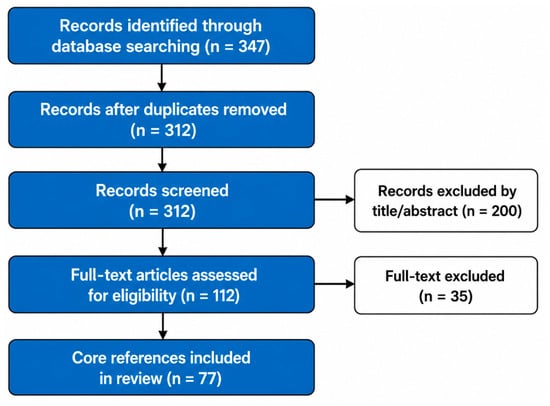
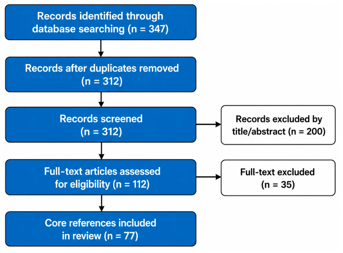
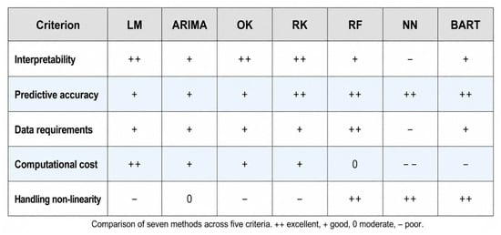
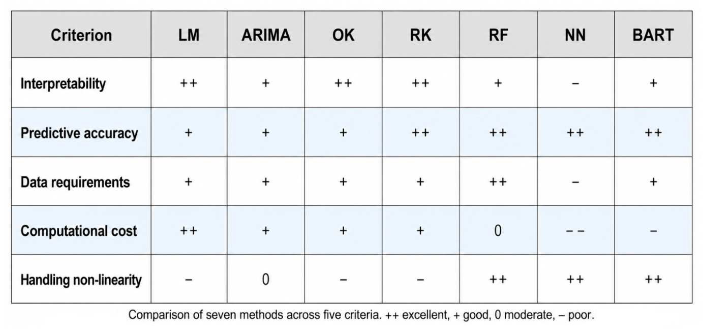
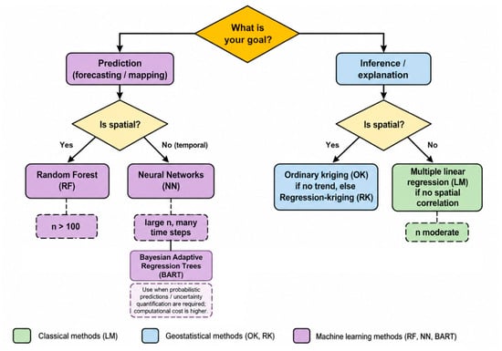
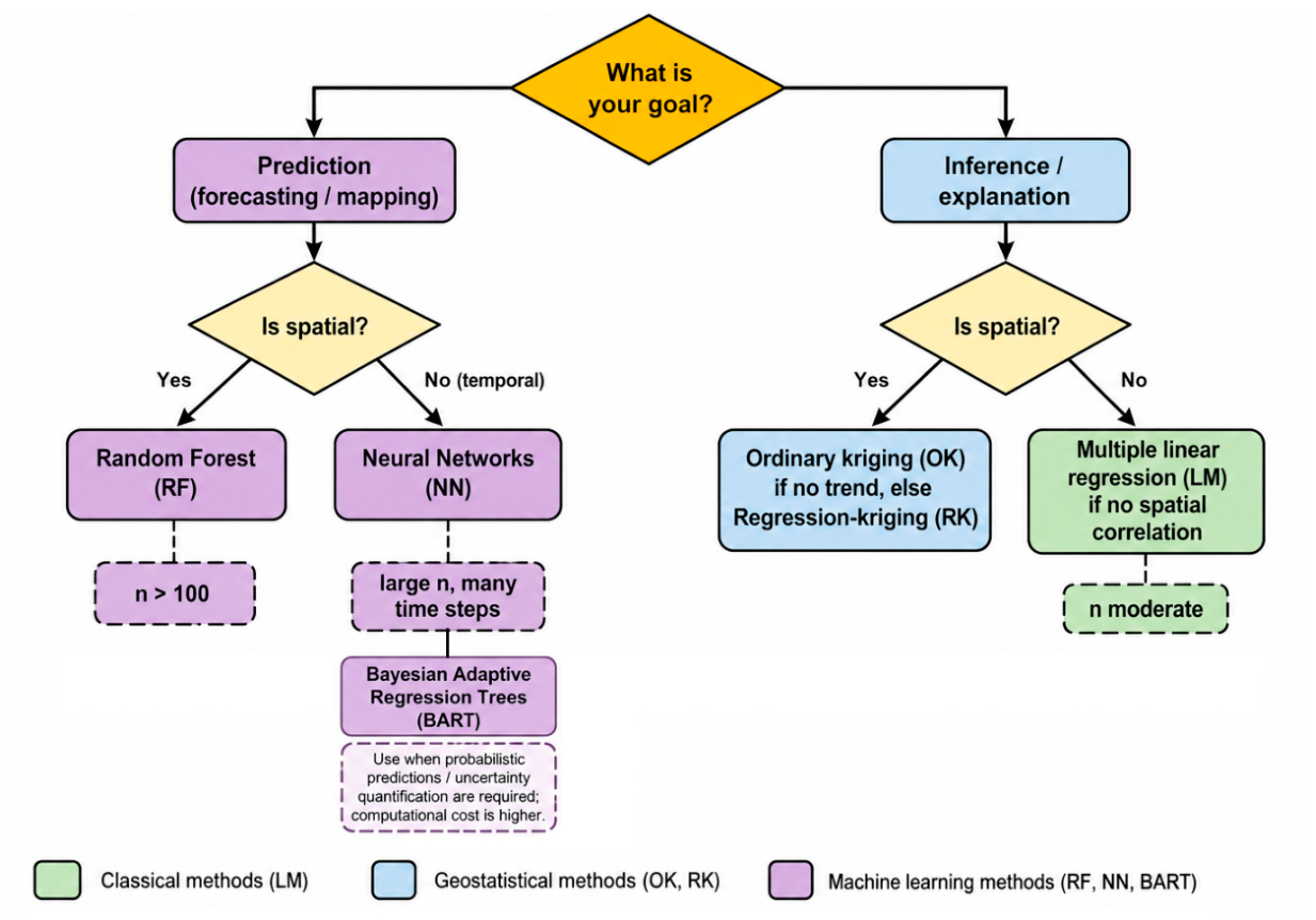
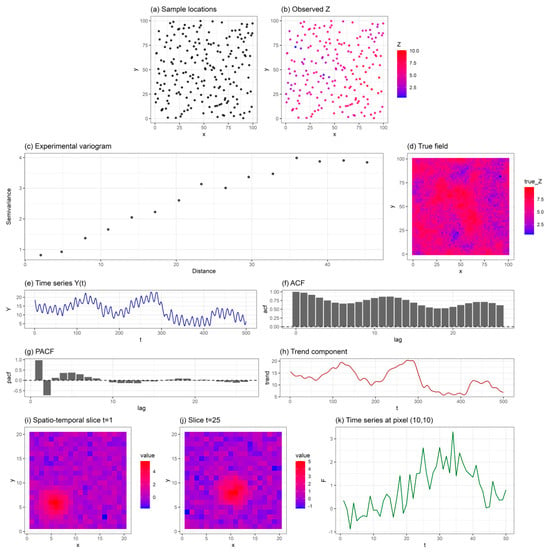
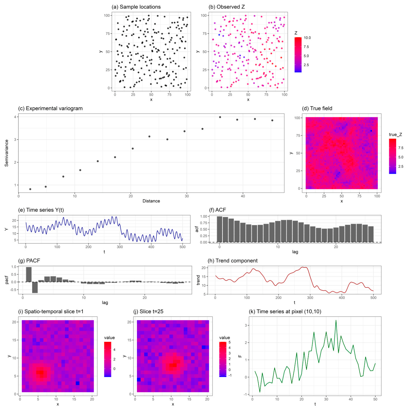
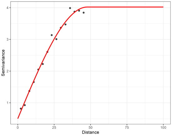
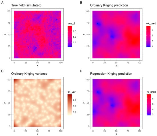
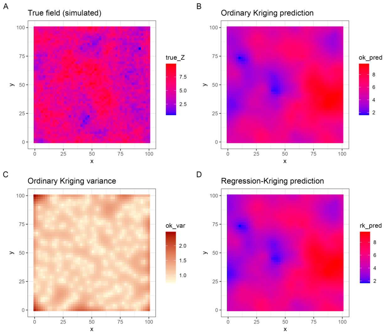
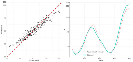
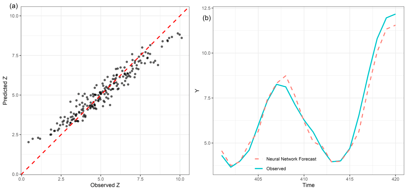
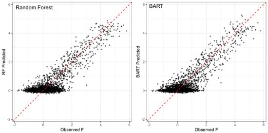
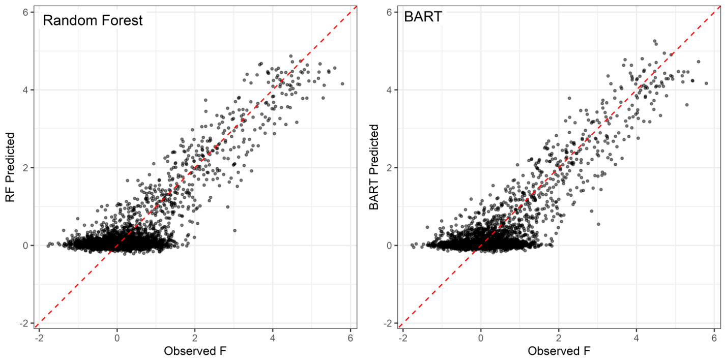
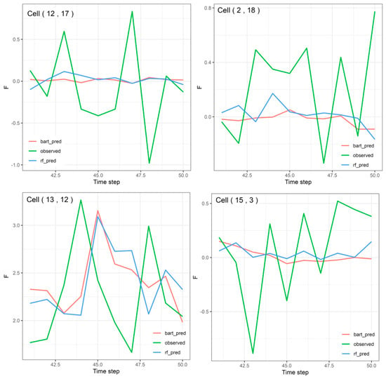
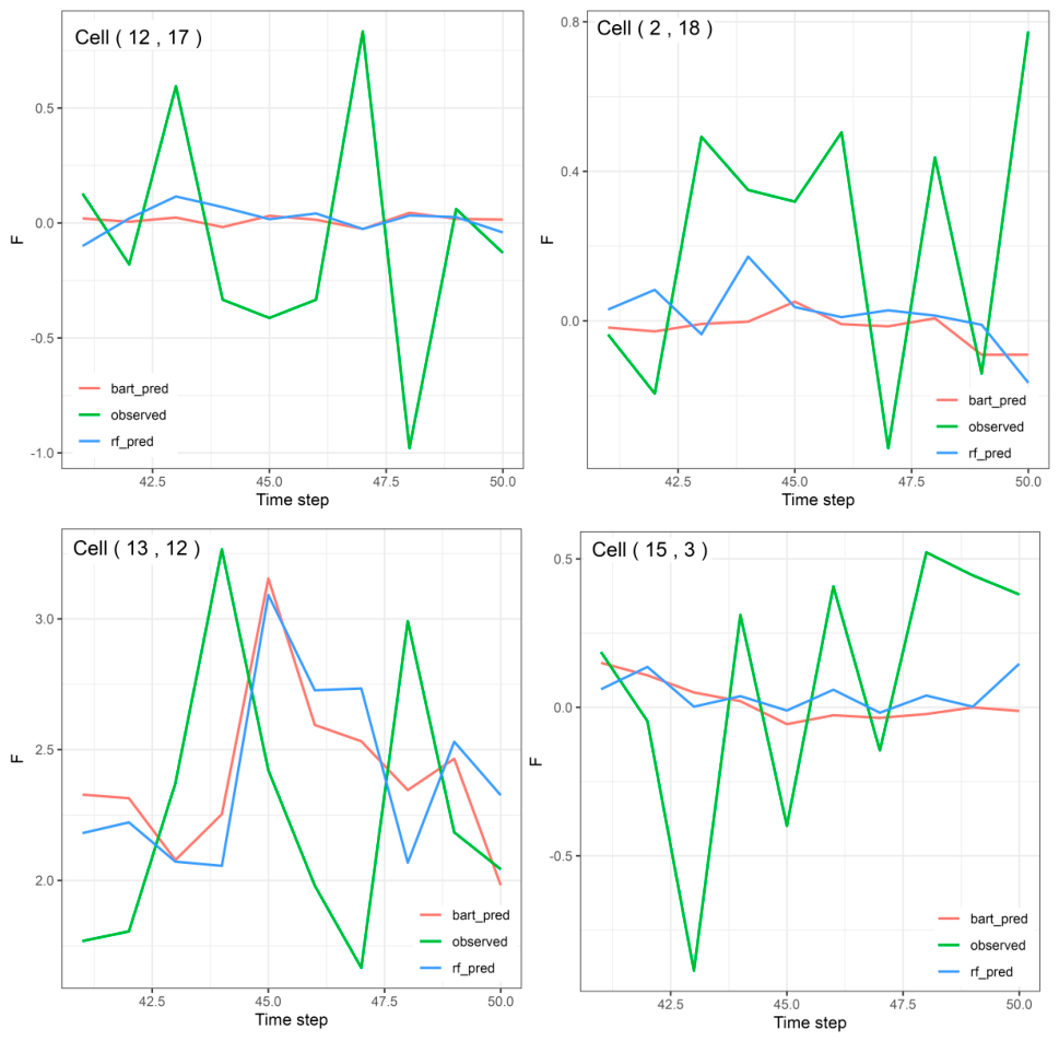
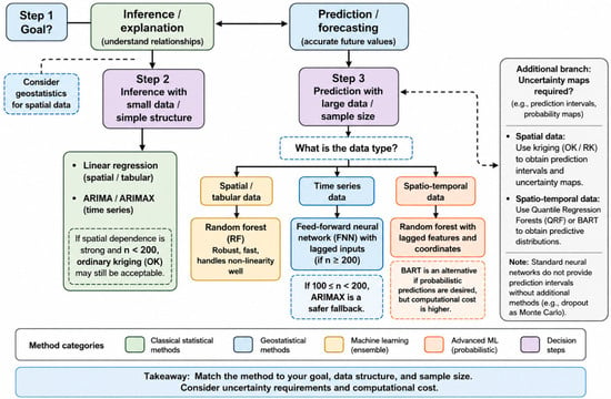
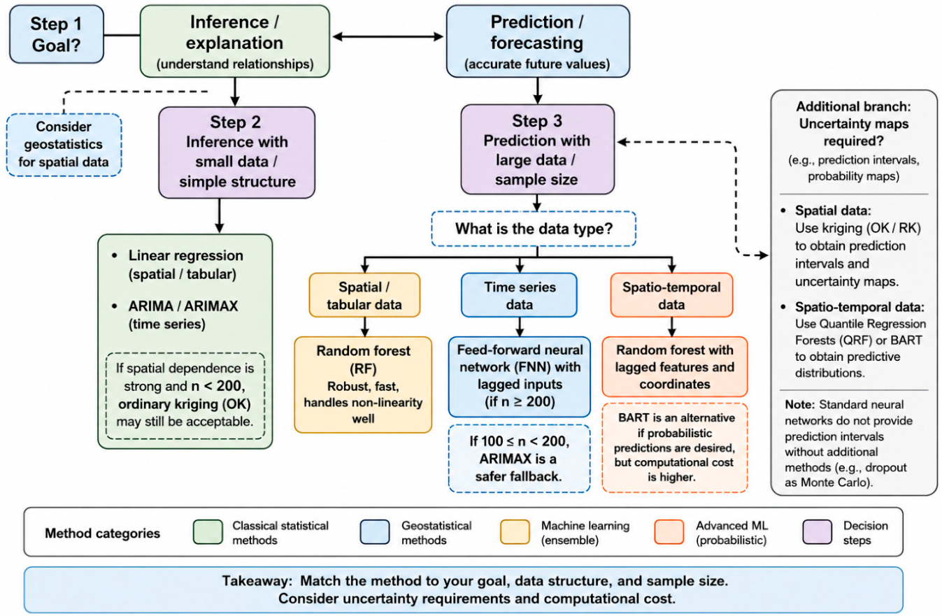

Disclaimer/Publisher’s Note: The statements, opinions and data contained in all publications are solely those of the individual author(s) and contributor(s) and not of MDPI and/or the editor(s). MDPI and/or the editor(s) disclaim responsibility for any injury to people or property resulting from any ideas, methods, instructions or products referred to in the content. |
© 2026 by the authors. Licensee MDPI, Basel, Switzerland. This article is an open access article distributed under the terms and conditions of the Creative Commons Attribution (CC BY) license.