Poststack Seismic Geomechanical Property Evaluation of the Pennsylvanian Strawn–Canyon Group in Salt Creek Field, Midland Basin, Kent County, West Texas

Abstract

Geomechanical properties of rock are essential components in designing hydraulic fracturing procedures. Although ultrasonic measurement methods are usually utilized to obtain static geomechanical properties of rocks in the laboratory, they are limited to borehole locations. To obtain spatial distribution of these properties, a 3D prestack seismic inversion process is employed to derive them dynamically. However, 3D prestack seismic datasets are less readily available compared to 3D poststack seismic. We present a methodology that integrates 3D poststack seismic and wireline log data using a machine learning workflow to compute the dynamic geomechanical properties, namely Young’s modulus (E), Mu-Rho (MR), and brittleness (BRI) volumes, and generate crossplots to characterize the Salt Creek carbonate reservoir in the Midland Basin, Kent County, Texas. Our results show that: (1) Based on the comparison of seismically (dynamically) derived E and BRI maps with litho-facies maps, the zones with the highest porosity (oolites) are characterized by low E and low BRI. (2) Each of these properties is linearly related to the photoelectric factor (PEF) log, which can indicate porosity and calcite richness within a mixed carbonate–siliciclastic system. (3) In a mixed carbonate and siliciclastic system, geomechanical properties, especially E, can be used to identify rigid rock layers within the reservoir and deduce possible lithologies. Finally, when prestack seismic data are unavailable, our workflow offers a quick and inexpensive method to generate dynamic geomechanical property maps to characterize hydrocarbon reservoirs using poststack seismic data and well logs.

1. Introduction

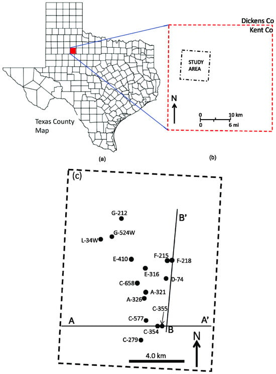
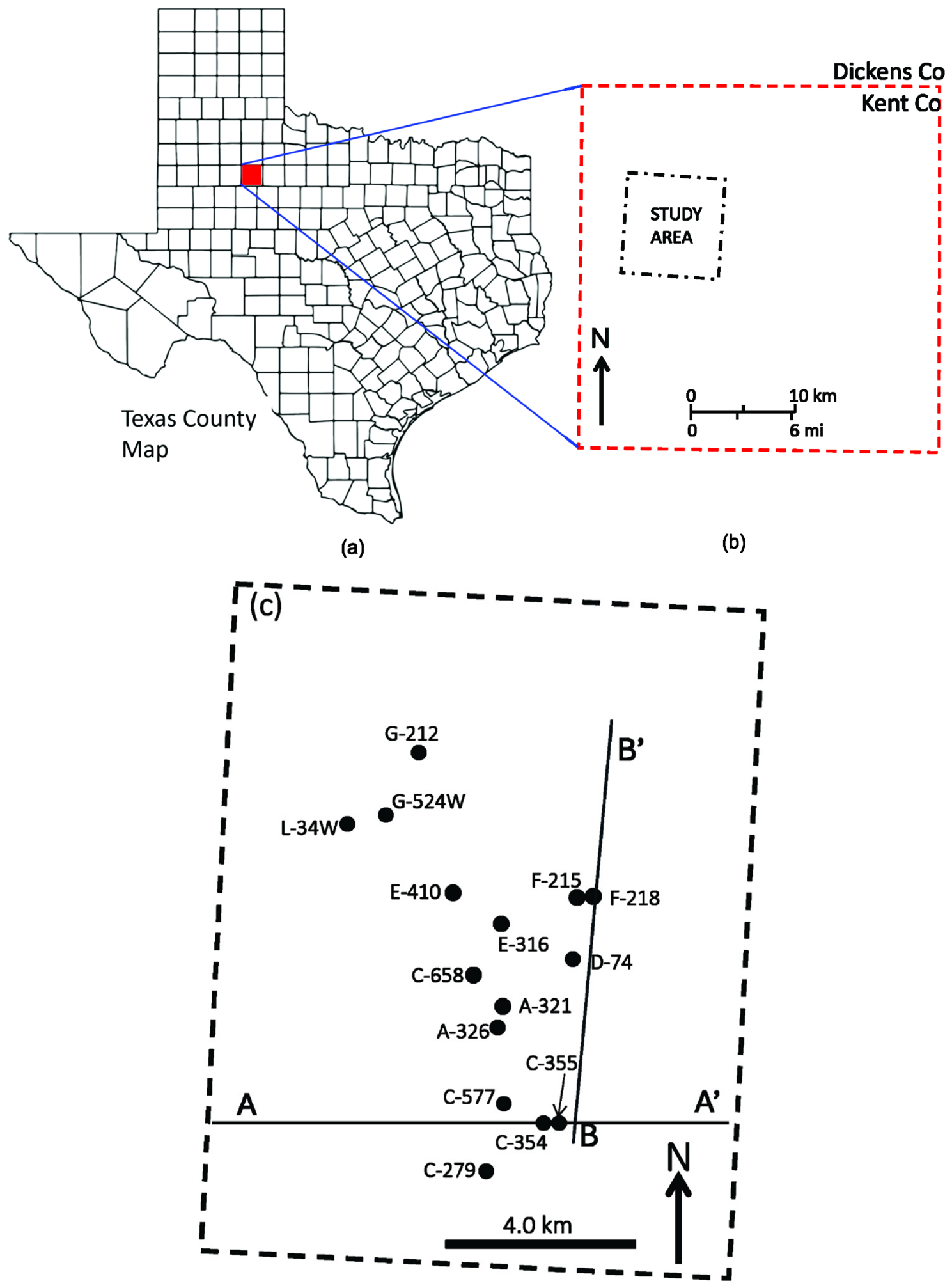
This article is an expanded version of an extended abstract of a conference paper, titled “Geomechanical property evaluation of the Pennsylvanian Strawn-Canyon Group using machine-learning methods: Insights from Salt Creek Field, Midland Basin, Kent County, West Texas”, which was presented at the George Brown Convention Center, Houston, Texas, on 26–29 August 2025 [1]. The area of investigation is Salt Creek Field, which is part of the Horseshoe Atoll located about 150 miles (~240 km) northeast of the Midland Basin, Kent County, West Texas (Figure 1 [2]). The intervals of interest are the Pennsylvanian Strawn, Canyon, and Cisco Groups, composed mostly of carbonates with few siliciclastic (shale) stringers. The porous zones consist of (a) skeletal packstones (b) algal boundstone, (c) oolitic grainstones, and (d) basal dark wackestone or mudstone [2,3,4,5]. Of these, the most porous intervals are oolitic grainstones with porosity values ranging up to 30% [2]. The entire Strawn and Canyon Group interval is capped by the Wolfcamp Formation, composed of thick shales with some interbedded thin carbonate layers [2,6]. Although Salt Creek Field has been producing since the 1950s, knowing the spatial geomechanical properties of the reservoir rocks would allow for better selection of drilling sites, drilling trajectories, and hydraulic fracturing designs to recover the remaining hydrocarbons. Several authors have discussed the use of geomechanical properties in fracture direction estimation. For example, ref. [7] discussed laboratory ultrasonic (dynamic) test equipment and procedures to obtain Young’s moduli and Poisson’s ratios for optimized fracture designs. The author provided equations for calculating dynamic Young’s modulus from borehole sonic logs and estimating the corresponding static Young’s modulus. Based on crossplots of Young’s modulus versus P-wave sonic (in km/s), the researcher derived an empirical relationship that can be used to calculate Young’s modulus given P-wave sonic velocities. Ref. [8] provided a comprehensive review of the theoretical basis of geomechanics and then went further to discuss the application of geomechanical properties in the characterization of the Fuja Field offshore Niger Delta. Working from Southwestern Iran, ref. [9] discussed modeling of geomechanical unit using seismic and well log data. The authors provided results of the application of Young’s modulus and Poisson’s ratio in optimizing drilling operation during the life cycle of hydrocarbon reservoirs in southwestern Iranian oilfields. Ref. [10] discussed the relationship between static Young’s modulus and seismic parameters (P-impedance, S-impedance, Lambda-Rho, and Mu-Rho). Based on crossplots, the authors derived equations that can be used to estimate static and dynamic Young’s modulus.

Figure 1. (a) Map of the State of Texas showing location of study area (red rectangle), (b) enlarged version of red rectangle showing location of study area in Kent County, (c) well database map showing lines of cross-sections A–A’ and B–B’ discussed in the text.

In addition to Young’s modulus computation, several other researchers (e.g., refs. [11,12,13,14,15]) have discussed brittleness of rock and its computation. Ref. [13] noted that different methods of computing brittleness have been suggested by different researchers based on different viewpoints, such as the strength of the rock, stress–strain, mineral composition, hardness, inner friction angle, elastic Young’s modulus, and Poisson’s ratio [13]. Irrespective of how it is computed or defined, brittleness is a key parameter in evaluating the risk of rock-burst, and rock fracturing to facilitate the production of shale gas and oil [13]. The above geomechanical properties are mostly computed from borehole wireline geophysical logs. However, boreholes are only available at discrete points and cannot be laterally representative of the entire rock body. Prestack 3D seismic inversion in which seismic trace locations can be as closely spaced as 12 m apart offers a way to obtain lateral distribution of geomechanical properties of rocks. However, generating dynamic geomechanical property volumes from seismic data requires three physical properties of the rock. These are density, P-wave acoustic impedance (Zp), and S-wave acoustic impedance (Zs) volumes. These parameter volumes are usually obtained from 3D prestack seismic datasets using simultaneous AVO inversion equation according to [16]

$$R_{PP }\left(\theta \right)= c_1{R}_P+ c_2{R}_S+c_3{R}_D$$

(1)

where R_PP is reflection amplitude at an incident point, (ϴ) is the angle of incidence, R_P is reflectivity due to changes in P-wave acoustic impedance, R_S is reflectivity due to changes in S-wave acoustic impedance, R_D is reflectivity due to changes in density, c₁ is a function of angle (ϴ), and c₂ and c₃ are functions of angle (ϴ) and velocity ratio (Vs/Vp). From Equation (1), Zp, Zs, and density volumes are obtained after several iterations. Once these three parameter volumes have been generated, the geomechanical properties of the rock can be computed including Lambda–Mu-Rho (LMR). The LMR inversion transforms the seismic data into geologically meaningful rock and fluid properties. It is very useful for differentiating lithologies (for example, sandstones and shales), identifying hydrocarbons, and assessing rock brittleness. Lambda-Rho, the product of incompressibility and density, is very sensitive to pore fluids such as gas and oil and porosity [17] but relatively unaffected by the rock matrix. Mu-Rho, the product of rigidity and density, indicates the shear strength of the rock. It is sensitive to the solid rock matrix, and it is independent of the pore fluids [17].

However, 3D prestack datasets are less common compared to 3D poststack seismic data which are readily available in the oil industry. The question now is, in the absence of prestack datasets, can we get the required three parameter volumes from poststack seismic data? If it is possible, how can we derive these parameter volumes from poststack datasets?

This paper discusses how to generate these volumes from poststack seismic data. The main novelty of the paper lies in a workflow that we constructed to generate the required volumes, and subsequently compute the lateral and temporal distribution of the reservoir geomechanical properties, including Young’s modulus and rock brittleness, in Salt Creek Field. Here, brittleness refers to the tendency of a rock to shatter or break suddenly with minimal or no bending, when subjected to pressure. We accomplished this feat by integrating 3D poststack seismic, wireline log data, multiattribute analysis, and machine learning probabilistic neural networks (PNNs).

2. Geology

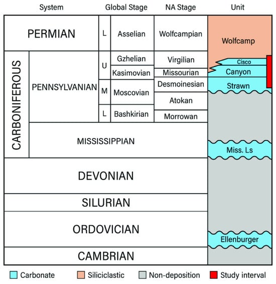
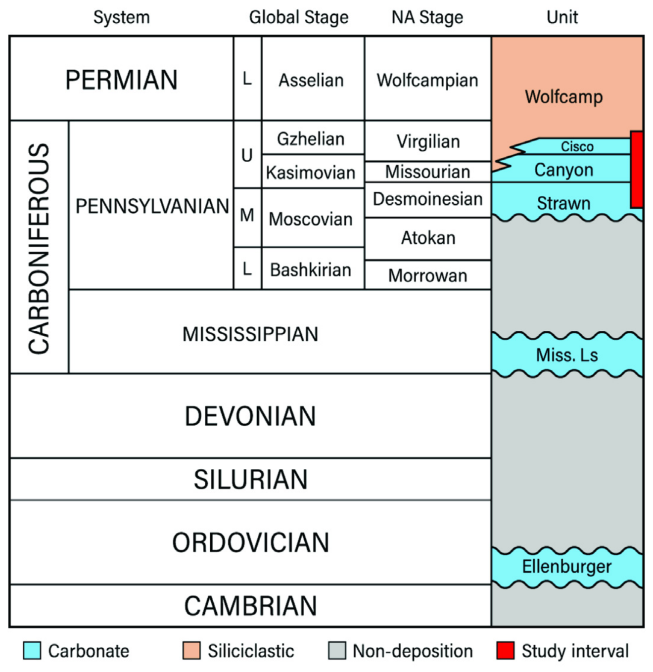
The schematic diagram (Figure 2) shows the various formations in the study area. The detailed geology of the Salt Creek Field has been discussed by many authors (e.g., refs. [6,18,19,20,21]) and as such, it will not be repeated here. However, it suffices to mention that the interval of interest is the Pennsylvanian Strawn–Canyon–Cisco Group, which is composed of mostly carbonates with some siliciclastic shale stringers (narrow red rectangle, Figure 2). The entire unit is part of the Horseshoe Atoll in the Midland Basin, Texas, made up of several algal reef buildups. Although hydrocarbons have been found within these carbonates, the most porous and productive zones within the Cisco and the Canyon are composed of oolitic grainstone, whereas, within the Strawn, the productive zones are the crinoidal grainstone and packstone [22]. In both cases, the productive zones are capped by the less porous and impermeable carbonates of algal boundstone and mudstone.

Figure 2. Schematic diagram showing the stratigraphy of the study interval composed of Strawn, Canyon, and Cisco Groups in Salt Creek Field (narrow red rectangle). Note: Letters “L”, “U”, “M” means lower, upper, and middle respectively. After [21] used with permission from Geosciences.

3. Database

There are 15 available wells in the study area, out of which nine were used to train and validate PNN (probabilistic neural networks). The suite of wireline logs consists of P-wave sonic logs, S-wave sonic logs, gamma ray logs, photoelectric factor (PEF) logs, density and neutron porosity logs, and resistivity logs. The poststack migrated 3D seismic dataset has a 90 × 90 ft (27.4 × 27.4 m) stacking bin size and is sampled at 2 ms interval. Cross-sections A‒A′ and B‒B′ (Figure 1c) display the results from poststack seismic inversion, PNN prediction, and geomechanical calculation processes discussed in Section 4.

4. Methods

4.1. Model-Based Acoustic Impedance Inversion

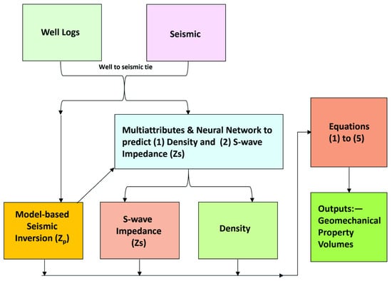
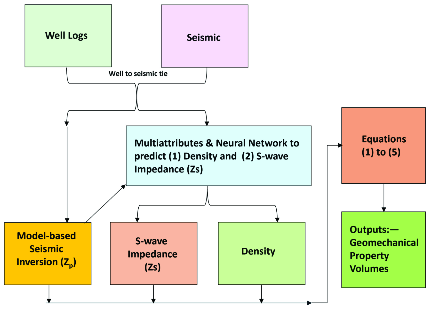
The computation of dynamic geomechanical properties from seismic data requires P-wave acoustic impedance Zp, S-wave impedance (Zs), and density volumes as necessary inputs into the algorithm. These volumes are obtained from 3D prestack seismic inversion. However, because of the lack of prestack data in our area, we designed a workflow (Figure 3) to generate these three required volumes. In this workflow we used HampsonRussell software (HRS) version 13.1. First, we performed poststack seismic inversion, and then multiattribute analysis and probabilistic neural networks (PNNs) to predict these volumes following methods discussed by (e.g.,ref. [21,23,24,25,26]). We utilized model-based poststack seismic inversion discussed by [23,24] to generate Zp volume. The first step was to generate a low-frequency model by applying a low-pass frequency filter to the wireline logs (acoustic impedance logs). This process was accomplished by interpolating the logs between the horizons utilizing the inverse distance method. Frequencies < 15 Hz are retained while those > 15 Hz are attenuated. We then used the low-frequency model combined with the extracted group wavelet to accomplish the inversion analysis process using the convolutional model expressed as [23]

$$S=W\ast R+Noise$$

(2)

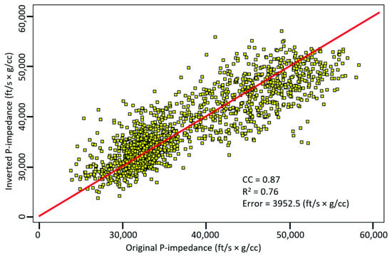
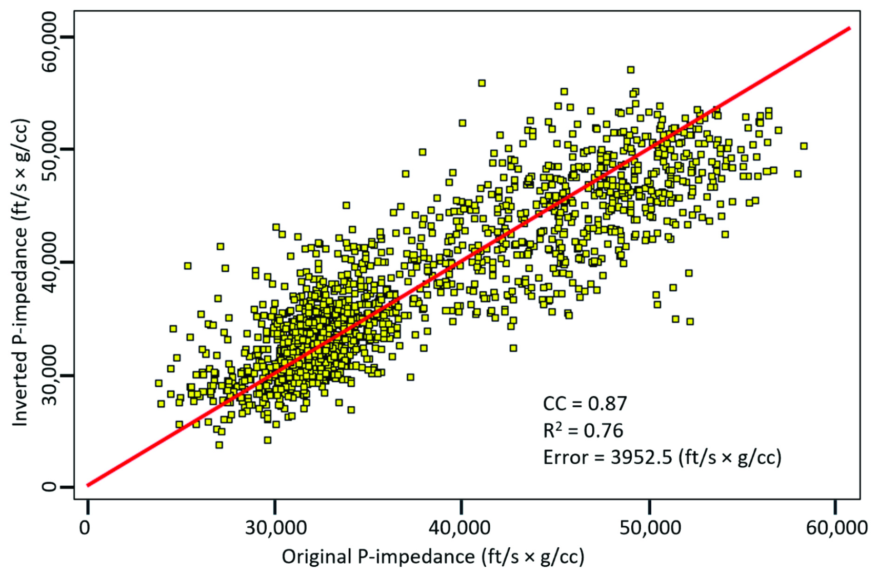
where S is the seismic trace, W is the wavelet, R is the reflectivities, and * is the convolution operator. The noise is random noise embedded within the seismic data. It does not correlate with the seismic signal and therefore is expected to cancel out. At this stage, optimal parameters are selected to execute the inversion procedure. This entails a repetition of the minimization process where the root mean-squared error between the inverted and actual impedance at every well location is computed. Once the minimum error has been determined, the process is terminated. Based on our investigation, the average R² from the crossplots between the inverted and actual Zp was 0.76 (Figure 4). The final Zp volume was obtained by applying the selected parameters to the entire seismic volume.

Figure 3. Schematic diagram showing workflow employed in this investigation. In this figure, density and Zs are outputs from multiattribute analysis and PNN processes. These volumes, together with Zp from poststack inversion, are input into Equations (2)–(6) to compute geomechanical properties.

Figure 4. Crossplots of inverted acoustic impedance (Zp) versus actual Zp showing R² of 0.76.

4.2. Multiattribute Analysis and Probabilistic Neural Networks (PNNs)

Having generated the acoustic impedance volume, we predicted Zs and density volumes using machine learning methods. To determine the sought-for log volumes (for example, Zs and density log volumes), the optimal number of seismic attributes are selected from a collection of attributes to train multiattribute and probabilistic neural network (PNN) using HRS version 13.1 software. Although we had 15 wells in the database, we used nine wells in the training and validation processes. The reason for this decision was because some of them either have poor quality logs or that the well stopped before reaching the objective interval, and thus, were excluded from the training processes. However, these nine wells are adequate for this project because of the small size of the field.

The collection of attributes consists of both internal attributes (that is, those that are generated on the fly from the seismic data by the software), and external attributes (i.e., previously computed volumes such as Zp, that are exported into the software by the user). The prediction process involves the determination of a statistical linear relationship between the sought-for log property (for example, density log), and seismic attributes employing the multilinear regression method expressed as [25]

$$Target Log\left(t\right)=w_{0 }+w_{1 }{\ast A}_{1 }\left(t\right)+w_{2 }{\ast A}_{2 }\left(t\right)+w_{3 }\ast A_{3 }\left(t\right)+ ..$$

(3)

where w_i are the weights, A_i(t) are the seismic attributes at each time sample, Target Log(t) is the sought-for log, and * is the convolutional operator [25]. The derived relationship is used to compute the sought-for log property for every sample and at every seismic trace location within the field. The algorithm is designed in such a manner that it employs the same datasets (well logs) for both the training and testing (cross validation). In the first stage (Round 1), the process begins with, for example, m wells, from which one is hidden, while the remaining (m − 1) are used in the training [25]. In Round 2, the well that was hidden is now brought back into the process for the next round of training; but in this training round, a new well is hidden. This procedure continues until every well has been involved in the training and validation processes. This means that every well also acts as a blind well.

During each round of the training, the least-squared error between the predicted and actual log is calculated and stored. The more attributes are added to the process, the more the error diminishes. However, adding more attributes could lead to overfitting the data and introducing noise and irrelevant attributes. Therefore, to avoid this problem, the cross-validation process is invoked [25]. This process identifies the location of the attribute at which the least-squared error started to increase rather than decreasing. At this stage, all the attributes used up to this point are taken as the required number of attributes needed to determine the sought-for log property. The accuracy is limited by the quality of the seismic data (signal-to-noise ratio and seismic resolution), quality of wireline logs, and well-to-seismic tie. To facilitate the predictability of Zs and density volumes, we loaded the inverted Zp volume from Section 4.1 and the neutron porosity NPHI volume that was previously determined from another project into the software as external attributes.

4.2.1. Prediction of Zs

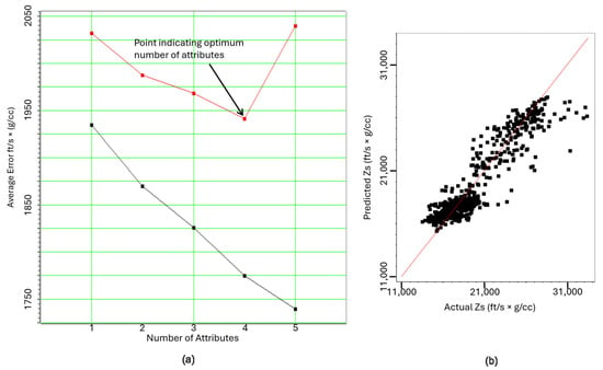
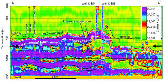
Based on the methods discussed in Section 4.2 above, we generated Zs volume. During the training and validation processes, the number of selected attributes to predict Zs was four (Figure 5a). We used the multiattribute linear regression method to select the attributes using an operator length of nine. That is, the number of samples employed in the convolutional process was nine. The algorithm selected the required attributes based on the order of relevance to the sought-for log property. The first attribute to predict Zs is neutron porosity (NPHI). Porosity has a strong linear relationship to impedance (velocity times density). The second attribute is Zp. Both Zp and Zs are also strongly related. The third attribute is integrated amplitude, which is related to acoustic impedance [27] and therefore is relevant to Zs. The fourth attribute is apparent polarity. This attribute is the signed reflection strength (amplitude envelope) which is also acoustic impedance-related [27,28] and thus is related to Zs. Having selected the attributes, we used the PNN algorithm to predict Zs using the following settings: an operator length of 9; the number of sigmas (smoothers) for training was 25; the sigma range was 0.1 to 3; the number of conjugate-gradient iterations was 20; and the pre-whitening used during training was 0.1%. We then generated crossplots of the predicted Zs versus actual Zs obtained during the training and validation processes to demonstrate the correlation between them (Figure 5b). The correlation coefficients for the training and validation processes are 0.92 and 0.89 respectively, and R² values are 0.85 and 0.79 respectively. Cross-section A–A’ through the predicted Zs volume (Figure 6) shows that the calcareous shale (Wolfcamp Formation) interval overlying the Canyon–Strawn Group is stratified. We interpret the strata that are associated with low Zs values as the shale-rich zones, while the strata with relatively high Zs values as the calcareous-rich zones. Below this interval is the Canyon–Strawn Group. This is the carbonate interval, and it is also stratified because of the different facies. We interpret zones that are characterized by low Zs values as the porous carbonate facies and those with high Zs values as low-porosity carbonates.

Figure 5. Crossplots from Zs prediction showing (a) average error versus number of attributes, and (b) predicted Zs versus actual Zs. Note: The red curve in a, is the plot of average error versus the number of attributes as one well is removed, while the black curve indicates the plot of average error versus the number of attributes using all wells during the training process. The red line in b, is line of best fit.

Figure 6. Cross-section A–A’ through predicted Zs volume. Note: Bold black arrows indicate timeline 970 ms at which time slice maps discussed in text were generated. This definition applies to subsequent cross-section figures. Note: Blue horizon is top of Strawn. Note: Dotted black outline indicate porous zones within the Strawn Group, while the dashed black outlines indicate outlines of the breccias on top of the Canyon discussed in the text. Note: There is a mismatch between the predicted Zs and the actual Zs in the inserted log within the Wolfcamp Formation. This is because Zs was under predicted at the shallow level where the beds are thin and below seismic resolution.

4.2.2. Prediction of Bulk Density

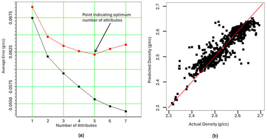
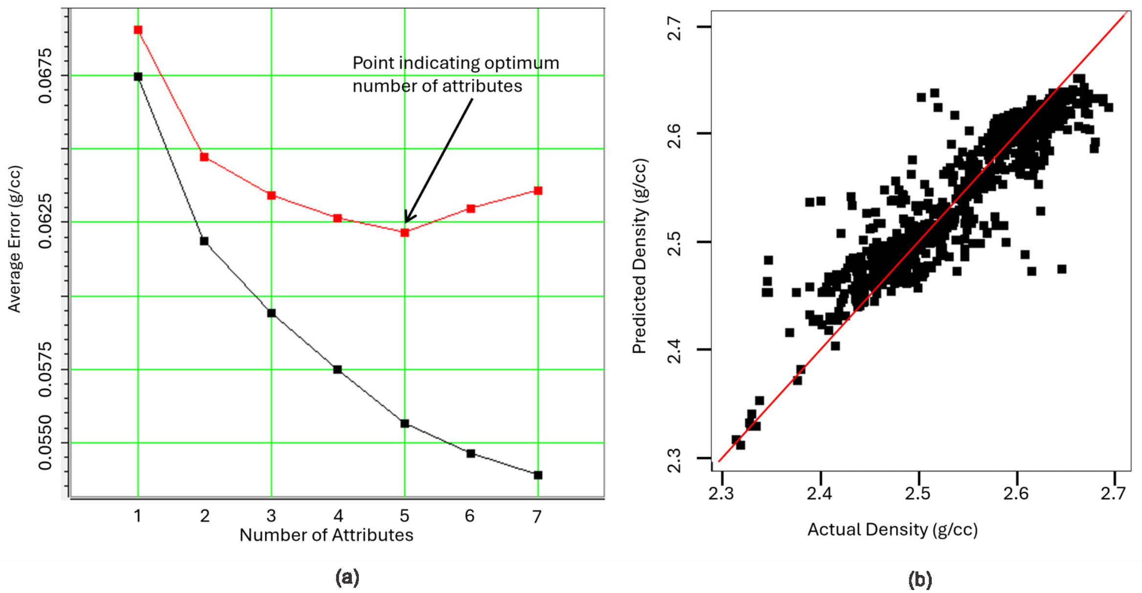
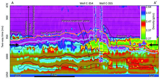
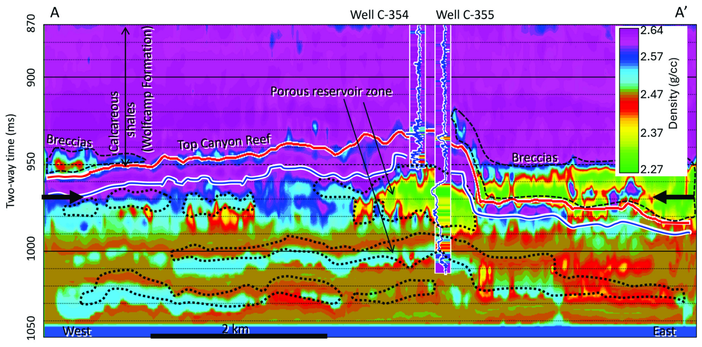
As in the prediction of Zs, multiattribute linear regression was used to select the required number of attributes, while PNN was used to predict the log using the same settings. During the training and validation processes to generate the bulk density volume, five attributes were selected based on the order of relevance to the log (Figure 7a). The first attribute is time, which is the time value of the seismic trace. It outlines a ‘slope function’ that can provide a trend to the computed reservoir property. The relevance of time to density can be viewed as the time of occurrence of events which are velocity related. The second attribute is neutron porosity (NPHI). Porosity is strongly related to density. The third attribute is Zp, which is also related strongly to density. The fourth and fifth attributes are the low-frequency (10 to 15 Hz) and high-frequency (10 to 50 Hz) filters suggesting the range of frequencies contained in the datasets. The low frequencies refer to highly porous zones, while the high frequencies refer to the low-porosity zones. Because frequencies are porosity related, and density is strongly related to porosity, therefore, frequencies are related to density. The crossplots of predicted versus actual density logs (Figure 7b) show that the correlation coefficients for the training and validation are 0.93 and 0.71 respectively, while the calculated R² are 0.86 and 0.5 respectively. Although R² for the validation is low, nevertheless, cross-section A–A’ through the density volume (Figure 8) clearly distinguishes between the breccias and the underlying Canyon–Strawn Group carbonates.

Figure 7. Crossplots from the prediction of density showing (a) average error versus number of attributes, and (b) predicted density versus actual density. Note: The red curve in a, is the plot of average error versus the number of attributes as one well is removed, while the black curve indicates the plot of average error versus the number of attributes using all wells during the training process. The red line in b, is line of best fit.

Figure 8. Cross-section A–A’ through density volume showing that the calcareous shale is denser than the underlying breccias and as dense as the underlying non-porous carbonate zones. Note: Blue horizon is top of Strawn. Note: the bold black arrows, dotted black outlines and the dashed black outlines are as defined in Figure 6. Note: There is a mismatch between the predicted density and the actual density in the inserted log within the Wolfcamp Formation. This is because density was under predicted at the shallow level where the beds are thin and below seismic resolution.

4.3. Computation of Dynamic Geomechanical Properties from Seismic Data

Having completed the multiattributes and PNN processes, the predicted density, Zs, and Zp volumes were input into Equations (4)–(8) to compute geomechanical properties at every seismic trace location to characterize the reservoir according to [11,15,29].

$$PR={\displaystyle \frac{0.5\ast {\left(\frac{Vp}{Vs}\right)}^2-1}{{\left(\frac{Vp}{Vs}\right)}^2-1}}$$

(4)

$$E={\displaystyle \frac{2\ast Z_s^2\ast \left(1+PR\right)}{Density}}$$

(5)

$$BRI=100\ast \left(w\ast {\displaystyle \frac{\left({PR}_{max}-PR\right) }{{PR}_{max}-{PR}_{min}}}+\left(1-w\right)\ast {\displaystyle \frac{\left(E-E_{min}\right)}{E_{max}-E_{min}}}\right)$$

(6)

where * denotes multiplication, PR is Poisson’s ratio, Zs is S-wave impedance, E is Young’s modulus, E_max and E_min are maximum and minimum Young’s modulus respectively, PR_max and PR_min are maximum and minimum Poisson’s ratio respectively, and w is aggregate weight of the minerals composing the rock. In this case, we assumed it to be 0.5 by taking the average of Poisson’s ratio and Young’s modulus [11]. We also computed Lambda-Rho and Mu-Rho using the following equations:

$$LR= Z_p^2-c\ast Z_s^2$$

(7)

$$MR=\mu \times \rho =Z_s^2$$

(8)

where LR is Lambda-Rho, MR is Mu-Rho, Zp is acoustic impedance, Zs is S-wave impedance, and c is assumed to be 2. Note that before deriving the geomechanical properties using seismic data, we first calculated the properties from the wireline logs (sonic velocity and bulk density logs) at every well location.

5. Results

5.1. Crossplots

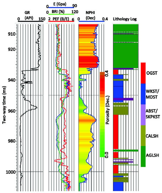
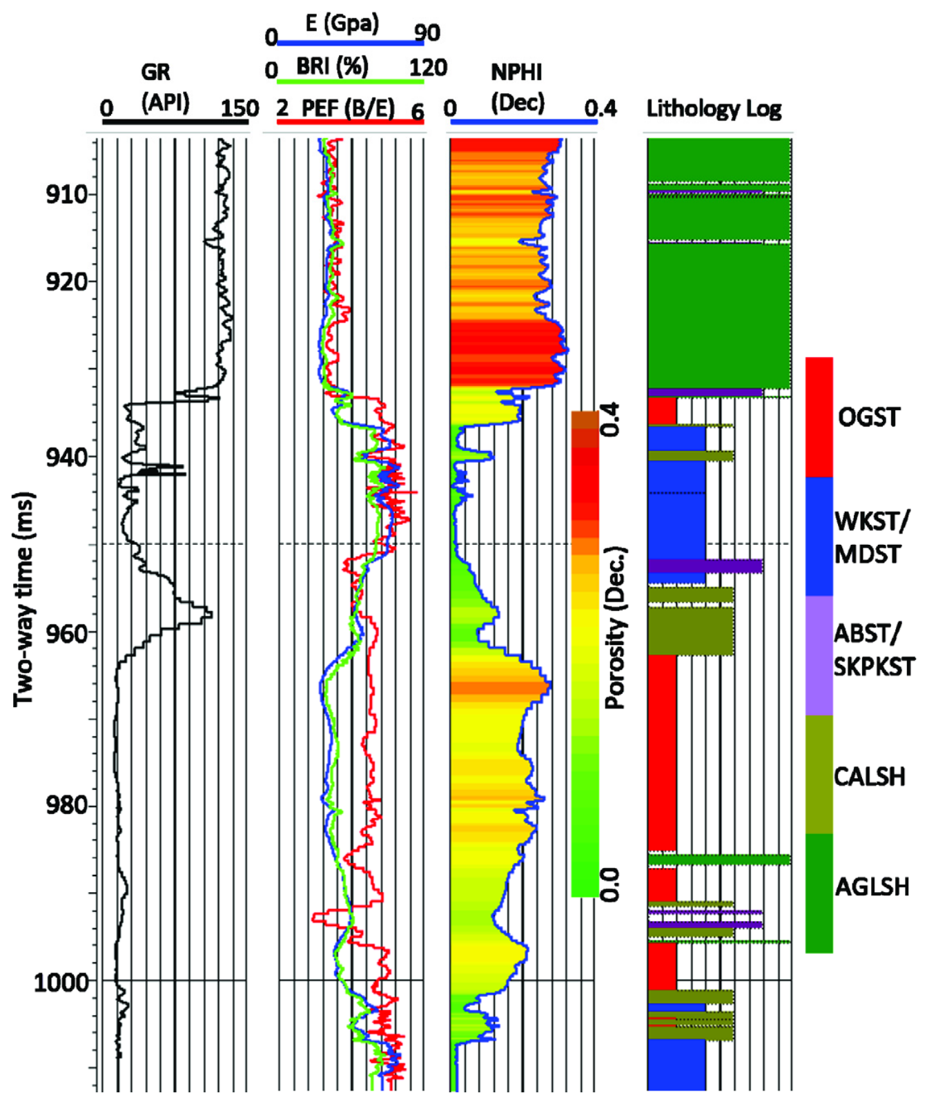
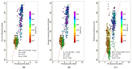
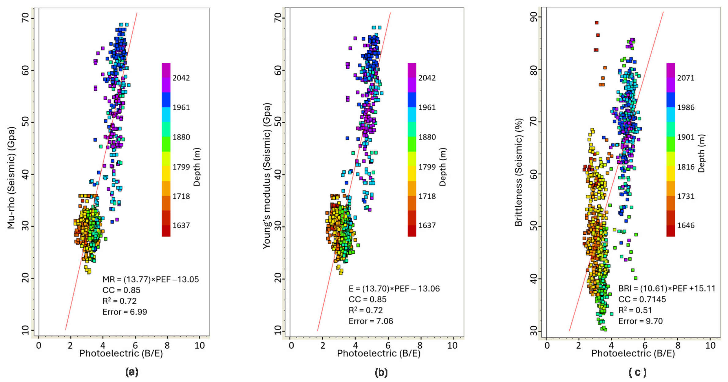
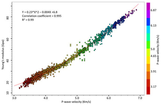
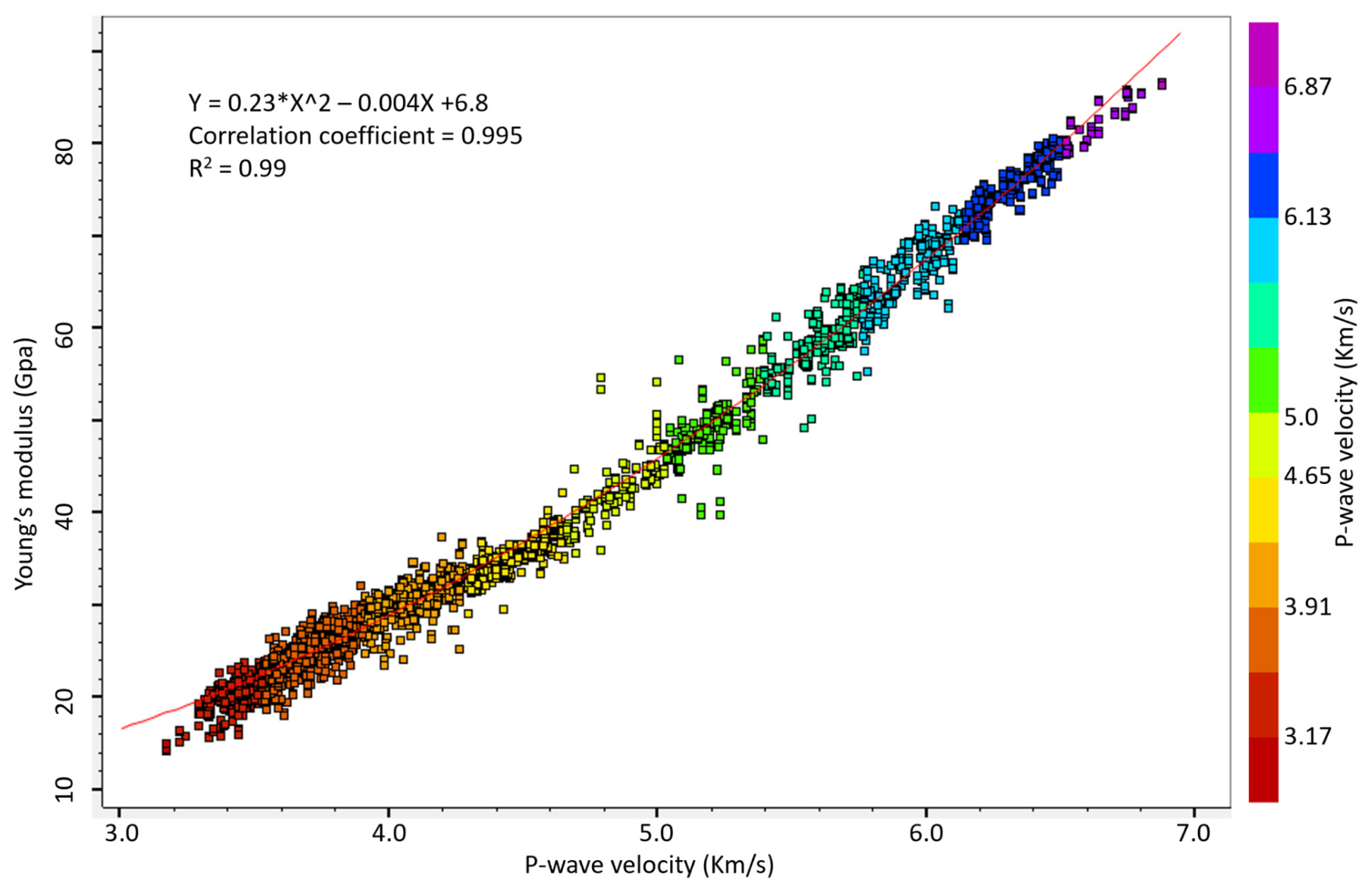
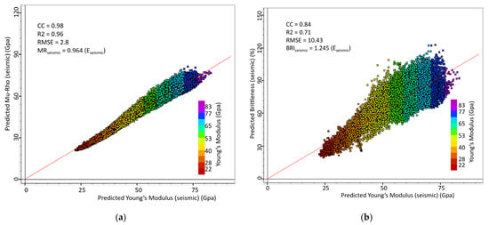
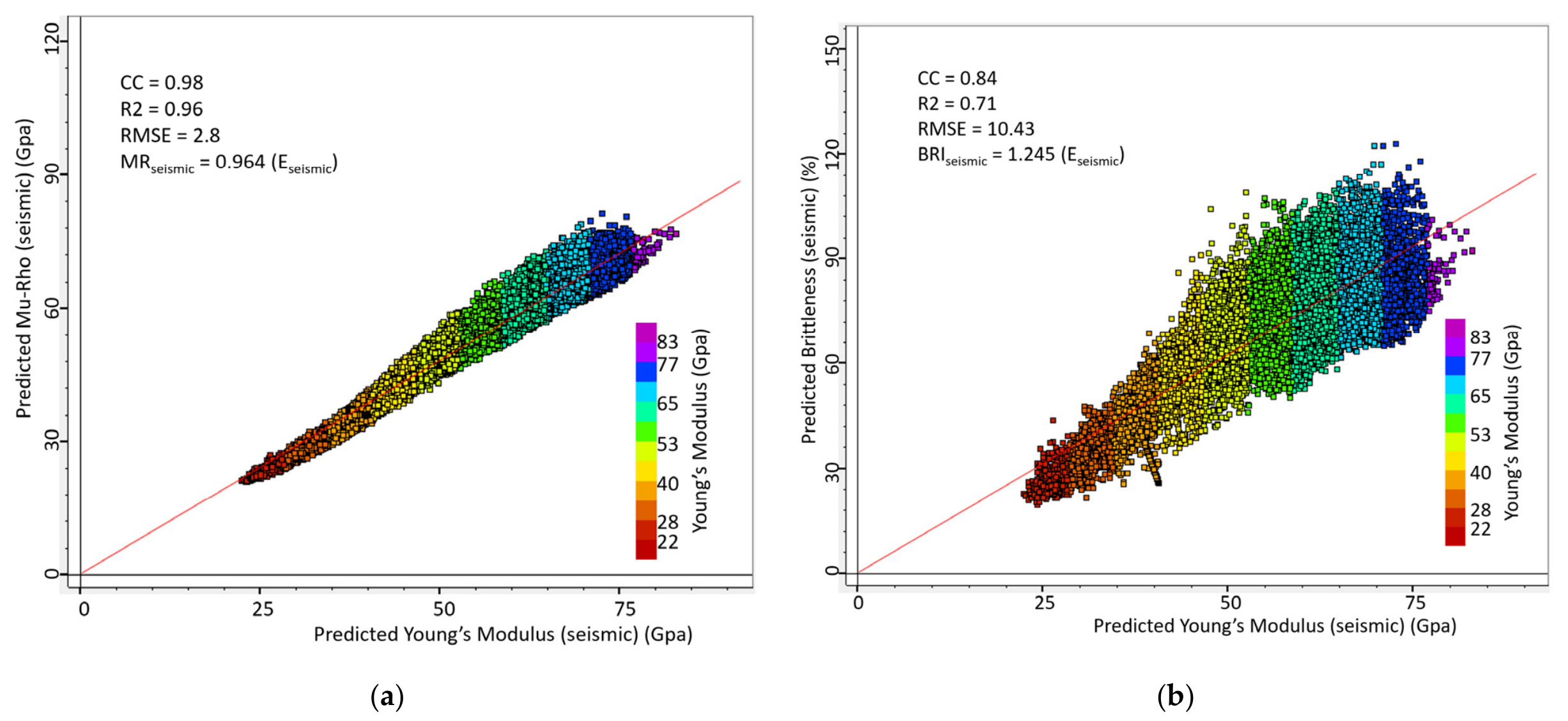
We demonstrate our results through series of crossplots, cross-sections, and maps obtained from the seismically derived geomechanical properties. First, we display log-calculated geomechanical property logs together with other logs such as gamma ray, photoelectric factor, and neutron porosity logs as well as the lithology log (Figure 9). We then generated crossplots of each of the geomechanical properties versus photoelectric factor logs (PEF) to derive a relationship between Young’s modulus and PEF and then relate lithology to brittleness. From this display, we observed that the PEF log appears to correlate well with E and BRI and that the most porous zones are characterized by unique PEF values [21]. By correlating PEF and geomechanical properties, the range of brittleness values characterizing the porous zones can be identified. Thus, we generated crossplots of E, MR, and BRI versus PEF color-coded in depth (Figure 10a–c). Both the plots of E and MR versus PEF show R² of 0.72. The plots indicate that E and MR increase as PEF increases (Figure 10a,b). We note here that although E and MR are strongly linearly related, they are not independent of each other since both depend on the same parameters or equations. As such, it suffices to interpret the results from E. Because high PEF values are indicative of high calcite concentrations (i.e., carbonate-rich rocks) [21], we infer that the high E not only suggests intervals of high rigidity but also provides insights into the lithological composition of the rocks. In addition, we note that the low-E (<37 GPa) zones occur at shallow depths (<6267 ft (1910 m)) whereas the high-E (>37 GPa) zones occur at depths > 6367 ft, ~1940 m) (Figure 10a,b). The vertical distribution of E values suggests that the less rigid rocks (that is, the siliciclastic) mostly occur at shallower depths, whereas the most rigid rocks (that is, the carbonates, characterized by high PEF) are located at greater depths. The plots of BRI versus PEF show similar results with R² of 0.51 (Figure 10c). Although the plot exhibits low R², it nevertheless shows that BRI increases as PEF increases. To demonstrate the relationship between E and P-wave, we present crossplots of Young’s modulus E versus P-wave sonic velocity obtained at one of the well’s locations (e.g., well F-215) (Figure 11). The plot shows a quadratic relationship with R² of 0.99 similar to [7]’s expression, suggesting a very good relationship. This observation should not come as a surprise since E is partly derived from P-wave [30]. To demonstrate that the seismically derived geomechanical properties are linearly related, we show crossplots of E versus MR and E versus BRI (Figure 12a,b). We observe that the plot of E versus MR has R² of 0.96 and that E and MR have almost identical or very similar values, suggesting that MR can be used/substituted in place of E and vice versa to characterize the rock. On the other hand, although the plot of E versus BRI has a very good relationship, R² is low, 0.71. Because brittleness is partly calculated from E and Poisson’s ratio, the correlation between E and brittleness is not fully independent just like between E and MR, hence the strong relationship that is observed between BRI and E. Figure 11 and Figure 12 were generated to be certain that our computed E and BRI agree with previously published results (e.g., refs. [7,30]).

Figure 9. Display of well logs plotted against time (ms) featuring photoelectric factor (PEF, red curve), gamma ray (black curve), neutron porosity, lithology log, and log-calculated geomechanical logs of Young’s modulus (E; blue curve) and brittleness (BRI; green curve). Note: OGST = Oolitic grainstone, WKST = Wackestone, MDST = Mudstone, ABST = Algal boundstone, SKPKST = Skeletal Packstone, CALSH = Calcareous shale, AGLSH = Argillaceous shale [1,22]. Note: The dashed horizontal line between two-way time 940 amd 960 ms, indicates time line 950 ms.

Figure 10. Crossplot of geomechanical property logs versus photoelectric factor log featuring (a) Young’s modulus E versus PEF, (b) Mu-rho versus PEF, and (c) brittleness versus PEF.

Figure 11. Crossplots of log-calculated Young’s modulus versus P-wave sonic velocity showing that the relationship between the two is quadratic. Note: The “*” in the equation is a multiplication sign.

Figure 12. Crossplots between geomechanical properties showing (a) Young’s modulus versus Mu-rho, and (b) Young’s modulus versus brittleness [1].

5.2. Cross-Sections

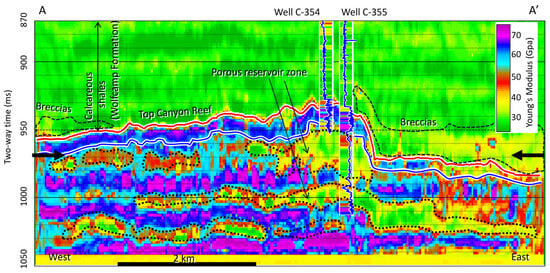
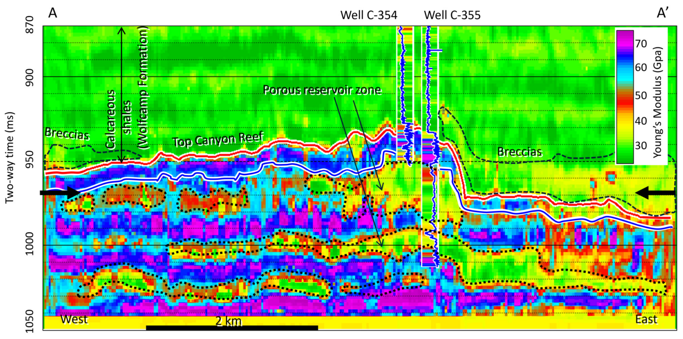
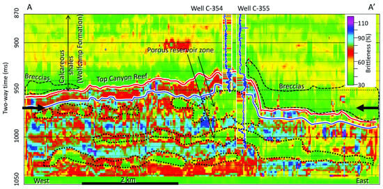
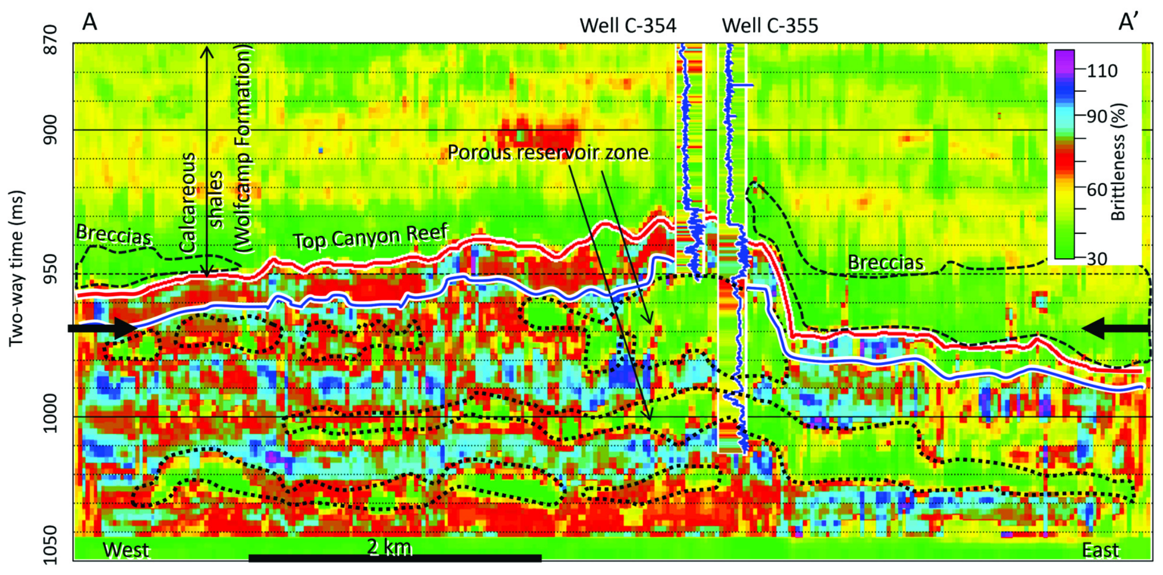
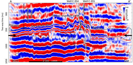
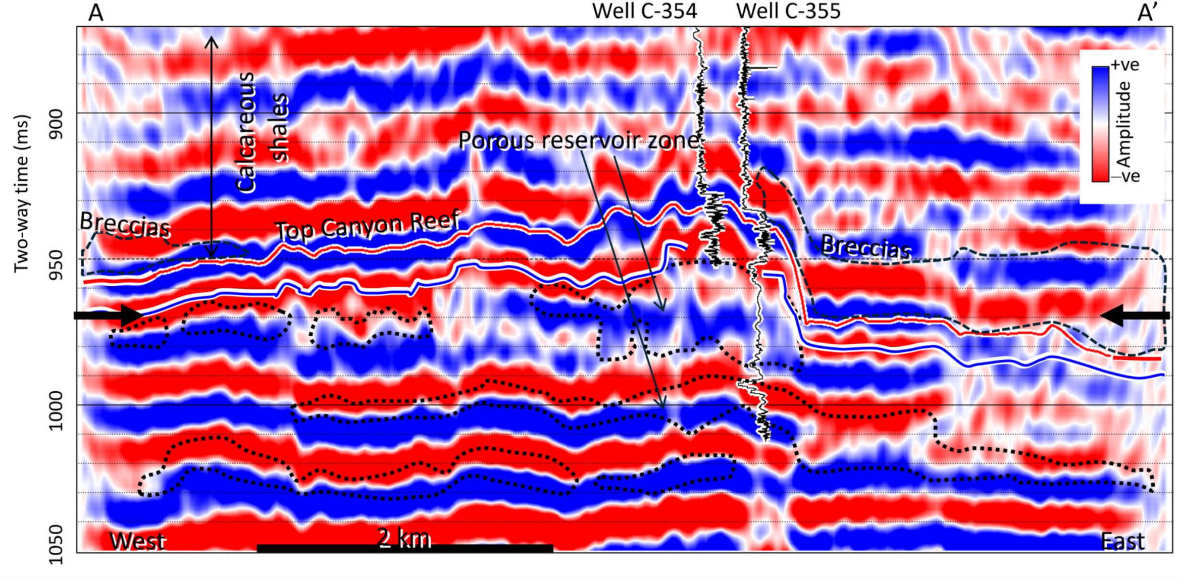
Cross-section A‒A′ through the predicted Young’s modulus (E) and BRI volumes featuring wells C-354 and C-355 (Figure 13 and Figure 14) respectively shows both vertical and lateral variations in E and BRI. Areas characterized by high E values are the light-blue-, blue-, and magenta-colored areas, while the low E zones are the green-, yellow-, red-, and brown-colored areas. Based on the inserted PEF log (blue curve), we note that the intervals of high PEF values, which are the calcite-rich and low-porosity zones, correspond to high E, while the low PEF values, which are the high-porosity zones, correspond to low E, as shown in Figure 13. Similarly, in the cross-section through the BRI volume (Figure 14), the high BRI zones correspond to low-porosity zones composed of high PEF. These two figures show the geomechanical stratification of the rocks composing the Strawn–Canyon interval. The low E values associated with the porous reservoir zone have values ranging from 25 to 45 GPa (Figure 9 and Figure 13). The zone is also characterized by moderately high PEF of about 4–4.8 B/E and low BRI values ranging from about 30 to 50% (Figure 9 and Figure 14). The corresponding cross-section through the 3D seismic volume (Figure 15) shows that both the porous and non-porous zones are hardly distinguishable. However, on transferring the porous outlines in E cross-section onto the seismic cross-section, we observe that the amplitudes corresponding to the porous zones at wells C-354 and C-355 appear to be distorted, low, and broad, compared to those in the non-porous zones. The change in amplitude suggests that major changes in acoustic impedance have occurred.

Figure 13. Cross-section A‒A′ through Young’s modulus (E) volume showing zones of low E (i.e., porous zone). Note: Blue horizon is top of Strawn. Note: The bold black arrows, dotted black outlines and the dashed black outlines are as defined in Figure 6. The mismatch between predicted E and actual E in the inserted log within the Wolfcamp Formation, occurred mostly at the shallow level where bed thicknesses are below seismic resolution.

Figure 14. Cross-section A‒A′ through brittleness (BRI) volume showing zones of low-BRI (i.e., porous zone). Note: Blue horizon is top of Strawn. Note: Bold black arrows, dotted black outlines and the dashed black outlines are as defined in Figure 6. The mismatch between predicted BRI and actual BRI in the inserted log within the Wolfcamp Formation, occurred mostly at the shallow level where bed thicknesses are below seismic resolution.

Figure 15. Cross-section A‒A′ through 3D poststack seismic volume showing zones of low, broad, and distorted amplitudes within the porous zone. Note: Blue horizon is top of Strawn. Note: Bold black arrows, dotted black outlines and the dashed black outlines are as defined in Figure 6.

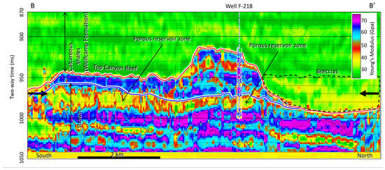
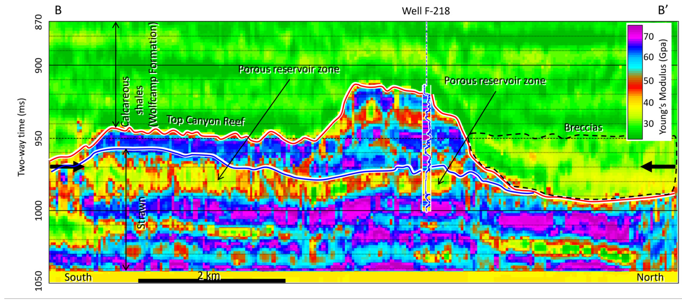
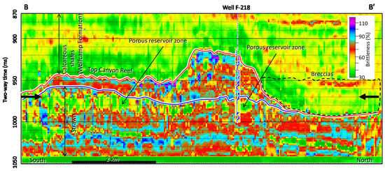
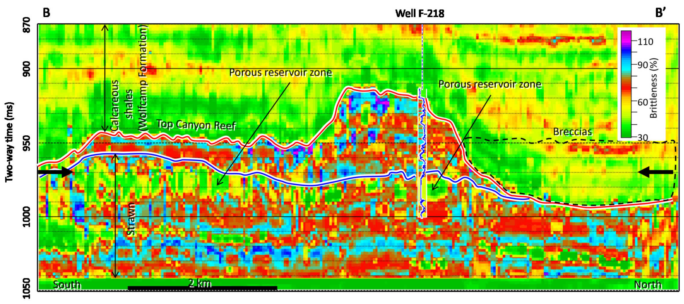
Cross-section B‒B′ through E volume taken at a blind well (F-218) location, which was not involved in the training (Figure 16), shows good agreement between the log-calculated E and the seismically derived E. The well log started just above the Canyon and thus, log values are not available for the Wolfcamp Formation at this location. In the Canyon interval, there are two intervals—one between 940 and 950 ms two-way time, and the other from approximately 963 ms two-way time to the top of Strawn—where the log-calculated E (shown on the inserted log) has higher values than the seismically derived E. In the Strawn interval, both the seismically derived E and log-calculated E show very good agreement. The same cross-section B‒B′ through BRI volume shows similar results (Figure 17). In this interval, both the seismically derived BRI and log-calculated BRI show very good agreement. Overall, the results show that both the log-calculated and seismically derived E and BRI are quite comparable.

Figure 16. Cross-section B–B’ through E volume showing comparison between seismically derived E and log-calculated E values at well F-218 location. Note: E log started from top of Canyon and thus, is not available within the Wolfcamp Formation. Note: The blue horizon is the top of the Strawn Group. Note: Bold black arrows, and the dashed black outlines are as defined in Figure 6. Note that top of the Strawn surface terminates against top of the Canyon to the north, suggesting that the top of the Canyon is an unconformity surface.

Figure 17. Cross-section B–B’ through BRI volume showing comparison between seismically derived and log-calculated BRI values at well F-218 location. Note: BRI log started from top of Canyon and thus, is not available within the Wolfcamp Formation. Note: The blue horizon is the top of the Strawn Group. Note: Bold black arrows, and the dashed black outlines are as defined in Figure 6. Note that top of the Strawn surface terminates against top of the Canyon to the north, suggesting that the top of the Canyon is an unconformity surface.

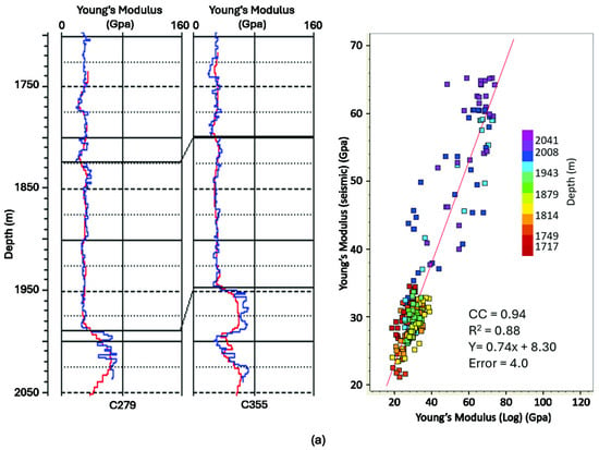
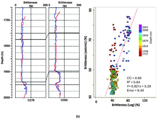
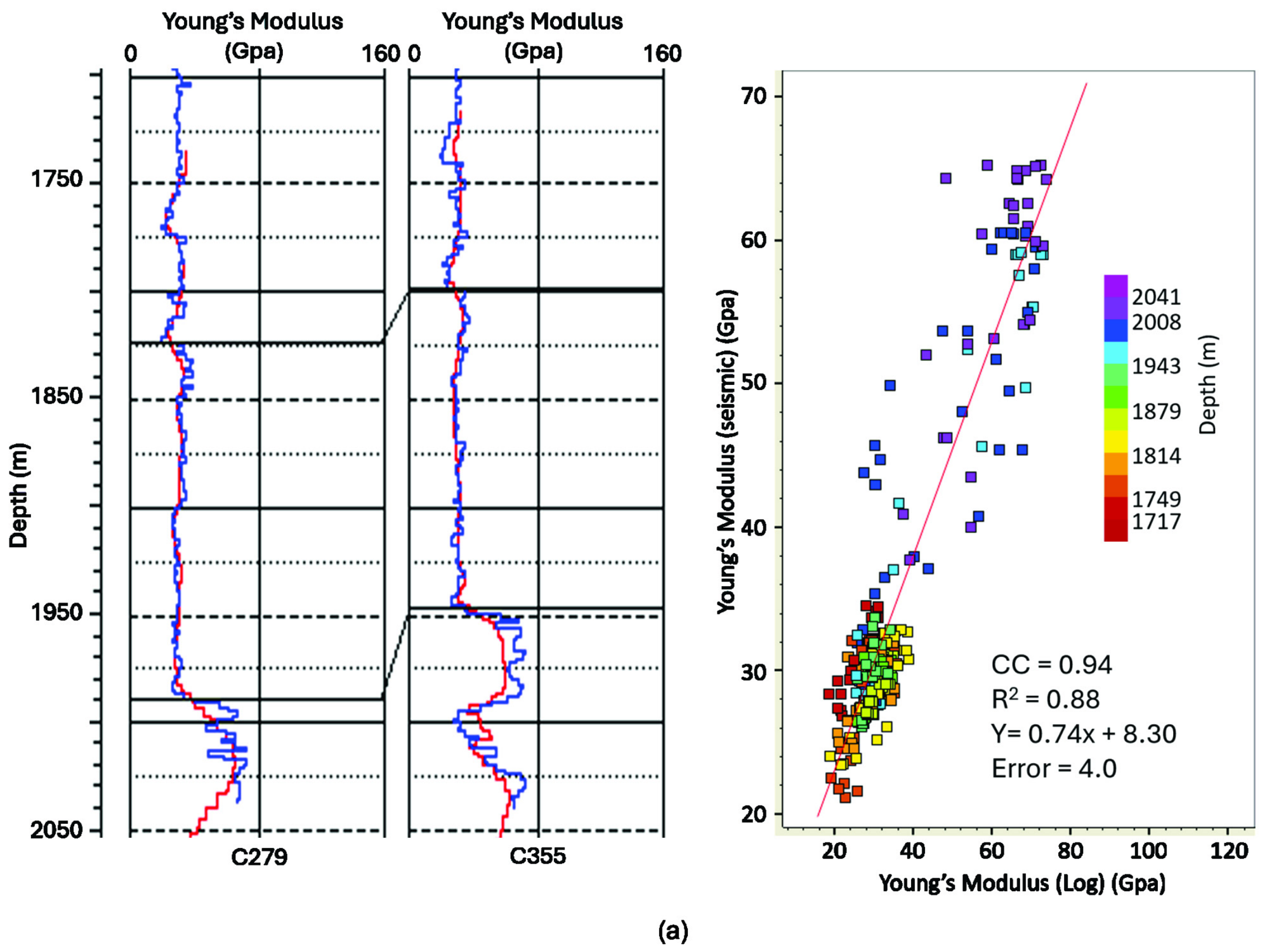
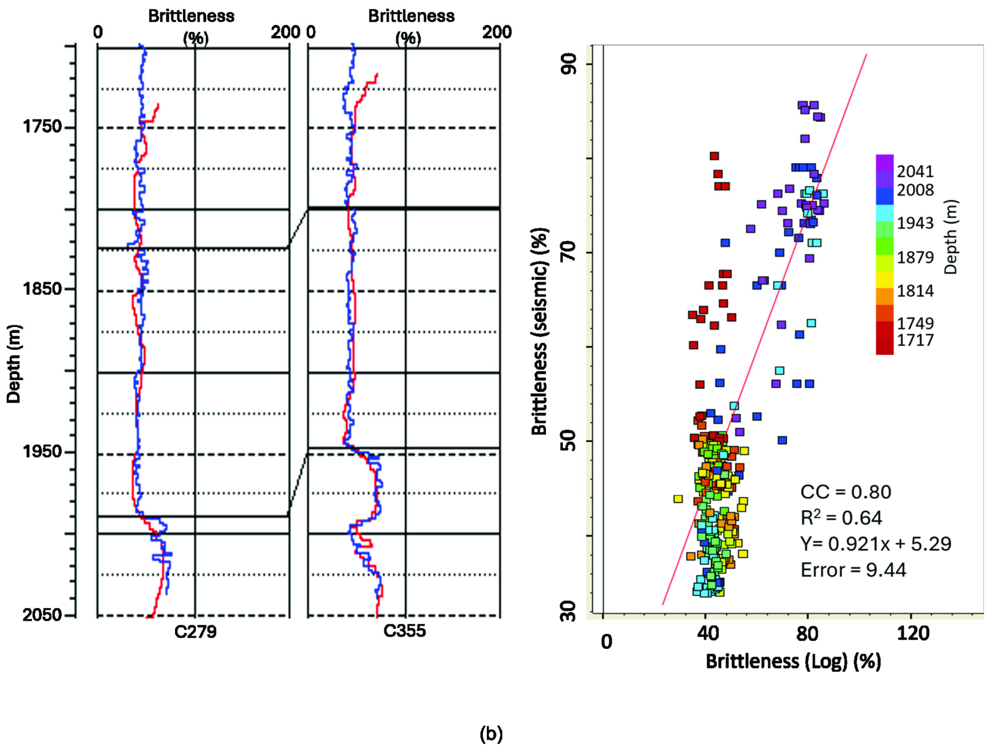
A crossplot to determine the relationship between the seismically predicted E versus the log-calculated E (color-coded in depth, Figure 18a) shows that there is a high degree of correlation, with a correlation coefficient of 0.94 and R² of 0.88 suggesting minimal error. However, the correlation coefficient and R² that we obtained for the BRI are low compared to E, being 0.8 and 0.64 respectively (Figure 18b). In addition, the crossplot suggests that most of the low-E zones occur at depths ranging from about 5578 to 6234 ft (~1700 to 1900 m). Although a few high E values are observed within this depth interval, the high-E zones occur at depths > 6234 ft (~1900 m) where the carbonates are dominant. We note that although the overall prediction is good, the R² value depends on the number of wells used in the crossplot and the errors associated with each of them. For example, using two wells (C-279 and C-355), the R² values for E and BRI were 0.88 and 0.64 respectively (Figure 18a,b), whereas using three wells (C-279, C-354, and C-355), the R² values for E and BRI were 0.85 and 0.53 respectively. The decrease in R² in this case suggests that the error associated with C-354 is relatively high.

Figure 18. Crossplots between log-calculated and seismically derived geomechanical properties featuring (a) log-calculated versus seismically derived Young’s modulus (right panel) and display of logs for two wells (left panel). (b) Log-calculated versus seismically derived brittleness (right panel) and display of logs for three wells (left panel). Note: In both a and b, left panel, blue curves are log-calculated logs, and red curves are seismically derived logs.

5.3. Comparison with Litho-Facies

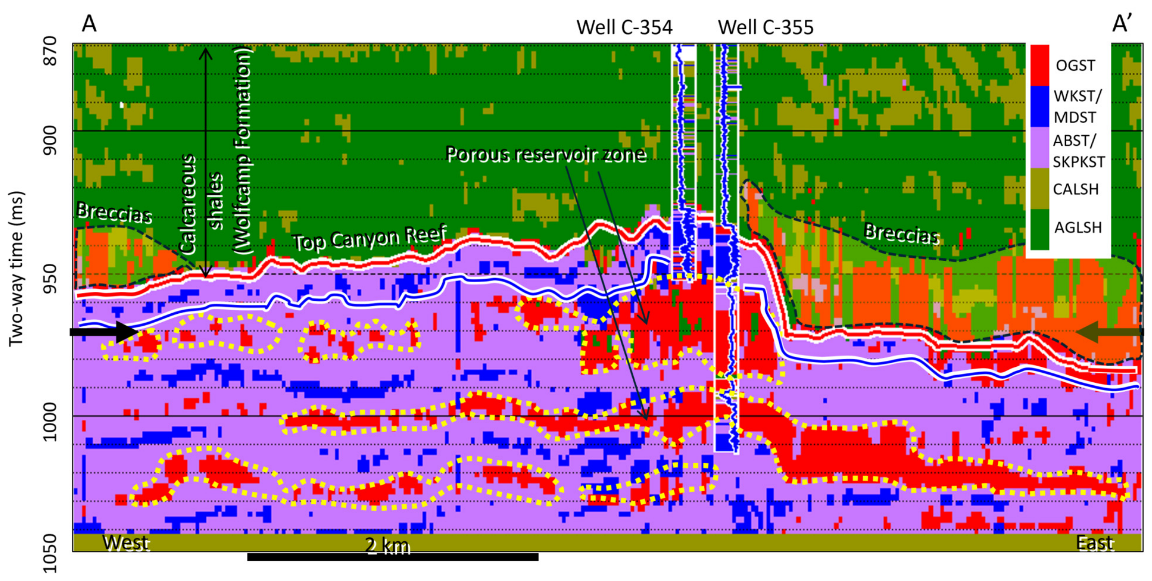
To associate the geomechanical properties with litho-facies, we generated cross-section A‒A′ through the litho-facies volume that we previously predicted in another project [22] (Figure 19). By transferring the dotted outlines of the low-E and low-BRI zones (Figure 13 and Figure 14) onto the litho-facies cross-section (Figure 19), we observed that these outlines correspond to porous oolitic- and crinoidal-grainstone zones (dotted yellow outlines). The high E values > 55 GPa (Figure 13) correspond to the less porous zones, which are skeletal packstone, wackestone/mudstone, and algae boundstone (cyan- and blue-colored zones, Figure 19). The caprock (calcareous shales, Figure 19) sitting on top of the red horizon is characterized by low E values of about ≤30 GPa except in the areas we have interpreted as breccias where E values range from ~30 to 45 GPa (Figure 13 and Figure 19). Although the porous interval is composed of carbonate, the associated high-porosity values make it less rigid compared to the surrounding rocks. We observed that at the shallow interval within the Wolfcamp Fornation, the predicted lithofacies differ from the actual lithofacies seen in the inserted log. The differences occurred due to: (1) at this shallow level, the strata are composed of many thin siliciclastic beds whose thicknesses are below seismic resolution. (2) The model lithology log used in the Bayesian classification, although was designed for the Strawn-Canyon Group, it was applied to the entire seismic volume. Thus, it did not properly capture the shallow zone; hence the presence of blank spaces and the misclassification seen in the inserted log at this level. However, this misclassification is inconsequential as it did not affect the results within the Strawn-Canyon Group which is the interval of interest.

Figure 19. Cross-section A‒A′ through litho-facies volume showing zones composed of oolitic grainstones (OGSTs). The section also shows the lateral distribution of different carbonate facies. Note: Carbonate breccias sitting on top of Canyon reef. Note: All abbreviations are as defined previously. Note: Blue horizon is top of Strawn. Note: OGST = Oolitic grainstone, WKST = Wackestone, MDST = Mudstone, ABST = Algal boundstone, SKPKST = Skeletal Packstone, CALSH = Calcareous shale, AGLSH = Argillaceous shale [1,23]. Note: Bold, black arrows, dotted yellow outlines and the dashed black outlines are as defined in Figure 6. The dotted yellow outlines here are black in Figure 6.

5.4. Extracted Geomechanical Property Maps

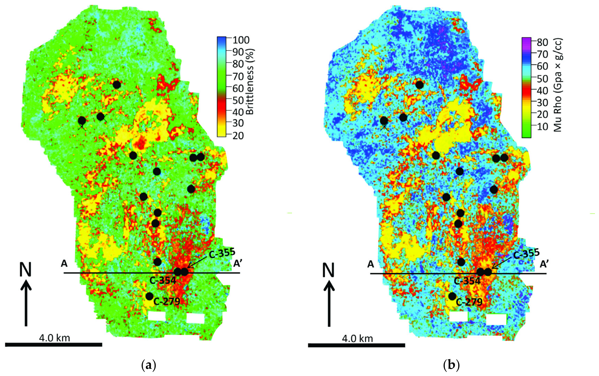
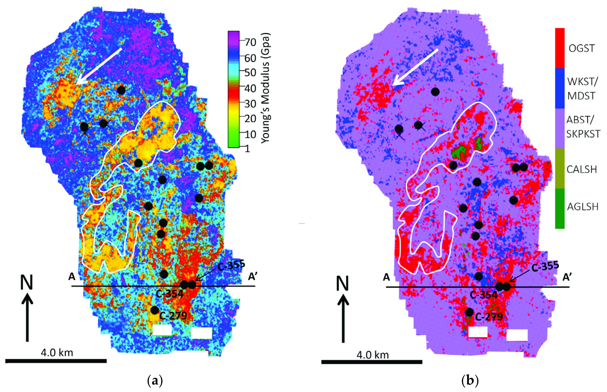
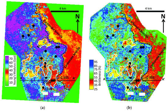
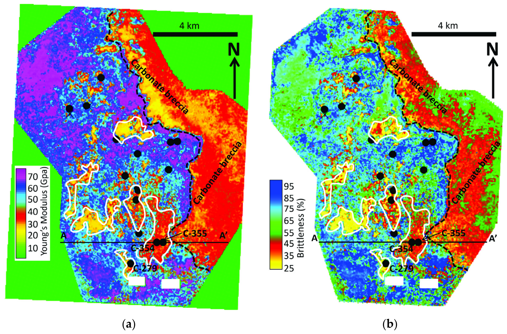
To demonstrate the areal distribution of geomechanical properties within the Salt Creek Field, we extracted E, MR, and BRI 5 milliseconds below the top of the Strawn Group (blue horizon). However, because these properties are related to each other as shown by crossplots (e.g., Figure 11 and Figure 12), the maps are almost identical. For example, a comparison of BRI and MR extracted maps (Figure 20a,b) shows the areas of low brittleness (red and yellow zones) and areas of low MR (yellow and red zones). The morphology of these zones on both maps is almost identical. Similarly, a comparison of both E and litho-facies [23] maps extracted 5 milliseconds below the blue horizon also shows the almost identical nature of the low-E zones (red and yellow areas, Figure 21a) and high-porosity zones (red areas, Figure 21b). Although there are several of these zones, by transferring the outline of one of them such as the white outline on the E map onto the litho-facies map (Figure 21b), we confirm that the low-E zones are almost identical to the porous zones on the litho-facies map. We note that porous zones such as the one identified by the white arrow, which no well has penetrated, could constitute potential areas, and thus, should be investigated further to confirm their structural integrity. On the E map, the brittle zones are the magenta, blue, and cyan areas (Figure 21a) with E values > 44 GPa, whereas, in Figure 21b, these areas are the blue and magenta zones (skeletal packstone, wakestone/mudstone). To determine the areal extent of the breccias on top of the red horizon (Figure 13, Figure 14 and Figure 19), we generated a time slice at 970 ms two-way time through the E and BRI volumes (Figure 22a,b). Like the previous E map (Figure 21), the time slice shows the lateral distribution of E and BRI values, highlighting outlines of low-E and low-BRI zones (porous zones). There are several of these porous zones of which six of them were outlined in solid white outlines. We note that west of the dashed-black line is the area occupied by the Canyon reef structure shown previously (Figure 20 and Figure 21), whereas, east of this line lies the area filled with carbonate breccias embedded within the calcareous shale characterized by low E from 25 to 44 GPa. Based on information from the regional geology of the Atoll area, the breccias have been interpreted to be carbonate sediments eroded from the Canyon reef topographic highs and redeposited on the flanks of the structure.

Figure 20. Extracted geomechanical property maps showing (a) lateral distribution of brittleness obtained 5 milliseconds below top of Strawn Group (blue horizon) and (b) lateral distribution of Mu-rho obtained 5 milliseconds below top of Strawn Group (blue horizon). Note almost identical morphology of porous zones (red and yellow zones) on both maps. Line A‒A′ is line of section along which cross-sections shown in Figure 13, Figure 14 and Figure 19 were generated. This definition applies to subsequent figures. Note: The black dots are well locations shown in Figure 1c. The blank rectangular zones indicate no data zones.

Figure 21. (a) Map of Young’s modulus extracted 5 milliseconds below top of Strawn Group (blue horizon) showing lateral distribution of porous zones (red and yellow areas), and (b) litho-facies map extracted 5 milliseconds below top of Strawn Group (blue horizon), showing lateral distribution of different carbonate facies particularly most porous facies—oolitic grainstone (OGST; red areas). Note: Thin white outline on both maps confirms almost identical morphology of porous zones identified by Young’s modulus and litho-facies. Solid white arrow indicates one of the untested porous zones within Strawn Group. All abbreviations remain as previously defined. Note: The black dots are well locations shown in Figure 1c. The blank rectangular zones indicate no data zones. White arrows indicate potential prospective zone discussed in the text.

Figure 22. Time slice at 970 ms through (a) Young’s modulus volume showing lateral distribution of porous zones (low E values), and (b) brittleness volume showing lateral distribution of porous zones (low-BRI values) in the area occupied by Canyon reef structure—area west of dashed-black line. Note: Areas east of dashed-black line are zones occupied by carbonate breccias. Note: The black dots are well locations shown in Figure 1c. The blank rectangular zones indicate no data zones.

6. Discussion

In this section, the focus is on the limitations of the workflow and the correlations between the seismically derived geomechanical and the litho-facies maps. Although our workflow would be highly beneficial to reservoir geoscientists, it does have some limitations due to associated errors. Some of the sources of errors could be traceable to the quality of the 3D seismic data (land datasets acquired in 1990s). For example, poor resolution seismic data with embedded random noise can adversely affect seismic-to-well ties, leading to the mismatch of well log data and seismic events. This problem is not a trivial issue because computed seismic attributes can be misinterpreted based on the well tie. Other sources of errors are poor quality well logs such as those from washout zones and those with spikes due to logging processes. These types of logs not only affect well-to-seismic ties but also introduce errors when employed in multiattribute and machine learning procedures. Compounding these errors are the ones associated with the multiattribute and PNN predicted volumes due to the non-optimal selection of predicting seismic attributes. These errors cumulatively degrade the final calculated geomechanical properties of the rock. This degradation is reflected in the low correlation coefficient and R² scores seen in the crossplots between the log-calculated and seismically derived BRI (brittleness). The BRI values are mostly affected probably because of the assumed 0.5 used to represent the aggregate weight (W) of the minerals in the rock in Equation (6). From Equation (6), in addition to the sources of errors discussed above, BRI calculation has two sources of errors, that is, error in E and Poisson’s ratio (PR). In this case, BRI would be affected more adversely than E, hence the lower R² score associated with BRI than E. However, if, for example, the actual weight (W) approaches 1, then BRI would depend wholly on (PR), which in turn depends solely on velocity ratio (Vp/Vs).

Next, we will discuss the correlation/similarity between the seismically (dynamically) derived geomechanical properties. The strong linear relationships between E and MR (Figure 18a) should not be a surprise because both properties depend on the square of S-wave impedance (Z_s) (refer to Equations (5) and (8)). The relationship between E and BRI (Figure 18b) is also very good because BRI is computed as the average of the sum of Young’s modulus E and Poisson ratio PR (Equation (6)) [11]. Hence, the extracted maps of E, MR, and BRI are very similar (Figure 20a,b and Figure 21a). We note that although the cross-sections from the litho-facies and E volumes are very similar, and that the corresponding maps are also very similar and have identical features, the two properties were derived differently and do not have any common parameter in the computation. For example, in predicting the litho-facies volume, which we generated in another project using Bayesian classification [22], the two key attributes that played key roles are photoelectric factor (PEF) and neutron porosity, and they were not calculated using any formula. Although neutron porosity was used to predict Zs and density volumes, it was not used in the computation of E and BRI. What can be said to be common to both E and litho-facies is that both are targeting the porous zones, which are the zones of low brittleness. Irrespective of the approaches, both E and litho-facies volumes successfully identified the porous zones. That the porous zones identified by both methods appear to be identical is a testimony to the accuracy of each method. Furthermore, it shows that Young’s modulus derived from seismic (dynamic) data can reliably be utilized to find porous as well as low-brittleness zones. In fact, ref. [7] argued that dynamically derived Poisson’s ratio and Young’s modulus should be used routinely in engineering studies.

Another point we would like to emphasize here is that in the absence of prestack datasets, poststack seismic procedures such as the one discussed in this paper would serve as a very good alternative to generate geomechanical properties. The justification of this approach is evidenced by the correlation between the seismically derived E and log-calculated E (Figure 18), and by the comparison between litho-facies and E maps (Figure 21a,b). Because poststack seismic datasets are more available to oil companies, the procedure discussed in this paper would offer those without prestack data a quick and inexpensive way to generate geomechanical maps to characterize and evaluate hydrocarbon reservoirs. In fact, there are occasions where bulk density log prediction results from poststack seismic and PNN have been found to be much more accurate than prestack results (e.g., ref. [31]).

7. Conclusions

We have shown that in the absence of prestack seismic inversion data, we can generate dynamic geomechanical properties using poststack seismic data combined with wireline logs and seismic attributes employing machine learning and neural network procedures. By computing the geomechanical properties (Young’s modulus (E), Mu-Rho (MR), and brittleness (BRI)) in a 3D sense and generating time slices, porous reservoir zones can be distinguished from non-reservoir zones. We observed that each of these properties correlates well with the photoelectric factor (PEF) log, which can identify calcite richness and porosity within a mixed carbonate–siliciclastic system [21]. In a mixed carbonate and siliciclastic system, geomechanical properties, especially E, can be employed to find the rigid rock layers within the reservoir and deduce porous zones and lithologies. However, the accuracy is limited by poor data quality and errors associated with the machine learning processes.

References

- Ogiesoba, O.C.; Palacios, F.C. Geomechanical property evaluation of the Pennsylvanian Strawn-Canyon Group using machine-learning methods: Insights from the Salt Creek Field, Midland Basin, Kent County, West Texas. In Proceedings of the SEG/AAPG International Meeting for Applied Geoscience & Energy, Houston, TX, USA, 25–28 August 2025; pp. 1781–1785. [Google Scholar] [CrossRef] [Scilit]
- Walker, D.; Jensen, J.; Zody, S.; Reid, S.T. Pennsylvanian cycle stratigraphy and carbonate facies control of reservoirdevelopment in the Salt Creek Field, Kent County, Texas. In Permian Basin Oil and Gas Fields: Innovative Ideas in Exploration and Development: West Texas Geological Society, Publication No. 90-87; Flis, J., Price, R., Eds.; AAPG: Tulsa, OK, USA, 1990; pp. 107–112. [Google Scholar]
- Heckel, P.H. Sea-level curve for Pennsylvanian eustatic marine transgressive-regressive depositional cycles along midcontinent outcrop belt, North America. Geology 1986, 14, 330–334. [Google Scholar] [CrossRef] [Scilit]
- Reid, A.M.; Reid, S.T.; Mazullo, S.J. Lowstand carbonate reservoirs: Upper Pennsylvanian sea level changes and reservoir development adjoining the Horseshoe Atoll: Southwest Section Meeting Abstracts. AAPG Bull. 1990, 74, 221. [Google Scholar] [CrossRef] [Scilit]
- Bishop, D.L.; Williams, M.E.; Gardner, S.E.; Smith, D.P.; Cochrane, T.D. Vertical conformance in a mature carbonate CO2 flood: Salt Creek Field Unit, Texas. In Proceedings of the Abu Dhabi International Conference and Exhibition, Abu Dhabi, United Arab Emirates, 10–13 October 2004. Paper Number SPE-88720. [Google Scholar] [CrossRef]
- Fairhurst, B.; Ewing, T.; Lindsay, B. West Texas (Permian) super basin, United States: Tectonics, structural development, sedimentation, petroleum systems, and hydrocarbon reserves. AAPG Bull. 2021, 105, 1099–1147. [Google Scholar] [CrossRef] [Scilit]
- Lacy, L.L. Dynamic rock mechanics testing for optimized fracture designs. In Proceedings of the SPE Annual Technical Conferences and Exhibition, San Antonio, TX, USA, 5–8 October 1997. [Google Scholar]
- Agoha, C.C.; Opara, A.I.; Okeke, O.C.; Okereke, C.N.; Onwubuariri, C.N.; Akiang, F.B.; Osaki, L.J.; Omenikolo, I.A. Integrated 3D geomechanical characterization of a reservoir: Case study of Fuja field, offshore Niger Delta, Southern Nigeria. J. Pet. Explor. Prod. Technol. 2021, 11, 3637–3662. [Google Scholar] [CrossRef] [Scilit]
- Sarem, M.N.; Riahi, M.A. Geomechanical unit modeling using seismic and well log data in one of the southwestern Iranian oilfields. J. Pet. Explor. Prod. Technol. 2020, 10, 2805–2823. [Google Scholar] [CrossRef] [Scilit]
- Sharifi, J.; Nooraiepour, M.; Amir, M.; Mondol, N.H. Developing a relationship between static Young’s modulus and seismic parameters. J. Pet. Explor. Prod. Technol. 2023, 13, 203–218. [Google Scholar] [CrossRef] [Scilit]
- Rickman, R.; Mullen, M.J.; Petre, J.E.; Grieser, W.V.; Kundert, D. A practical use of shale petrophysics for stimulation design optimization: All shale plays are not clones of the Barnett shale. In SPE Annual Technical Conference and Exhibition; SPE: Richardson, TX, USA, 2008. [Google Scholar] [CrossRef] [Scilit]
- Wood, D.A. Brittleness index predictions from lower Barnett Shale well-log data applying an optimized data machine algorithm at various sampling densities. Geosci. Front. 2021, 12, 101087. [Google Scholar] [CrossRef] [Scilit]
- Liu, C.; Du, L.; Zhang, X.; Wang, Y.; Hu, X.; Han, Y. A new rock brittleness evaluation method based on the complete stress-strain curve. Lithosphere 2021, 2021, 4029886. [Google Scholar] [CrossRef] [Scilit]
- Xia, Y.; Zhou, H.; Zhang, C.; He, S.; Gao, Y.; Wang, P. The evaluation of rock brittleness and its application: A review study. Eur. J. Environ. Civ. Eng. 2022, 26, 239–279. [Google Scholar] [CrossRef] [Scilit]
- Lee, J.; Lumley, D.E. Predicting shale mineralogical brittleness index from seismic and elastic property logs using interpretable deep learning. J. Pet. Sci. Eng. 2023, 220, 111231. [Google Scholar] [CrossRef] [Scilit]
- Fatti, J.; Smith, G.; Vail, P.; Strauss, P.; Levitt, P. Detection of gas in sandstone reservoirs using AVO analysis: A 3D Seismic Case History Using the Geostack Technique. Geophysics 1994, 59, 1362–1376. [Google Scholar] [CrossRef] [Scilit]
- Goodway, B.; Chen, T.; Downton, J. Improved AVO fluid detection and lithology discrimination using Lamé petrophysical parameters: “λp”, “µp”, and λ/µ fluid stack”: From P and S inversions. Recorder 1997, 22, 7. Available online: https://csegrecorder.com/articles/view/improved-avo-fluid-detection-and-lithology-discrimination-using-lame-petrop (accessed on 20 July 2026).
- Alnazghah, M.; Kerans, C. Late Pennsylvanian glaciation: Evidence of icehouse conditions from Canyon and Cisco Units, Midland Basin, Texas. Mar. Pet. Geol. 2018, 94, 198–211. [Google Scholar] [CrossRef] [Scilit]
- Sur, S.; Soreghan, G.S.; Soreghan, M.J.; Yang, W.; Saller, A.H. A record of glacial aridity and Milankovitch-scale fluctuations in atmospheric dust from the Pennsylvanian tropics. J. Sediment. Res. 2010, 80, 1046–1067. [Google Scholar] [CrossRef] [Scilit]
- Ewing, T.E. Tectonics of the Wast Texas (Permian) Basin: Origins, structural geology and later modification. In Anatomy of a Paleozoic Basin: The Permian Basin, USA; AAPG Memoir 118; Ruppel, S.C., Ed.; AAPG Memoir: Tulsa, OK, USA, 2019; Volume 1, pp. 63–96. [Google Scholar]
- Ogiesoba, O.C.; Palacios, F.C. Photoelectric factor characterization of a mixed carbonate and siliciclastic system using machine-learning methods: Pennsylvanian Canyon and Strawn Reef Systems, Midland Basin, West Texas. Geosciences 2025, 15, 3. [Google Scholar] [CrossRef] [Scilit]
- Ogiesoba, O.C.; Palacios, F.C. Probabilistic Neural Network and Bayesian Characterization of Salt Creek Field, Midland Basin, Kent County, Texas. Geoenergy Sci. Eng. 2026, 263, 214536. [Google Scholar] [CrossRef] [Scilit]
- Russell, B.H. Introduction to Seismic Inversion Methods: Society of Exploration Geophysicists; Course Notes, No. 2; SEG Books: Tulsa, OK, USA, 1988; Volume 2, 176p, ISBN 0931830656, 9780931830655; Available online: https://books.google.com.au/books/about/Introduction_to_Seismic_Inversion_Method.html?id=uUIx-89aifwC&redir_esc=y (accessed on 2 August 2026).
- Russell, B.; Hampson, D. A comparison of poststack seismic inversion methods. In Proceedings of the SEG International Exposition and Annual Meeting, Houston, TX, USA, 10–14 November 1991; pp. 876–878. [Google Scholar]
- Hampson, D.; Schuelke, J.; Quirein, J. Use of multiattribute transform to predict log properties from seismic data. Geophysics 2001, 66, 220–236. [Google Scholar] [CrossRef] [Scilit]
- Chopra, S.; Sharma, R.K.; Keay, J. Seismic reservoir characterization of Bone Spring and Wolfcamp Formations in the Delaware Basin—A case study: Part 1. Interpretation 2020, 8, T927–T940. [Google Scholar] [CrossRef] [Scilit]
- Tana, M.; Koehler, F.; Sheriff, R.E. Complex seismic trace analysis. Geophysics 1979, 44, 1041–1063. [Google Scholar] [CrossRef] [Scilit]
- Abatzis, I.; Kerr, J. Near spatial visualization techniques in tectonic and stratigraphic interpretation optimize reservoir delineation of the Roar Field, Danish North Sea. In Proceedings of the SEG Technical Program Expanded Abstracts, Houston, TX, USA, 10–14 November 1991; pp. 263–265. Available online: http://onepetro.org/SEGAM/proceedings-pdf/SEG91/SEG91/SEG-1991-0263/1998406/seg-1991-0263.pdf/ (accessed on 15 July 2026).
- Mavko, G.; Mukerji, T.; Dvorkin, J. The Rock Physics Handbook; Cambridge University Press: Cambridge, UK, 2009. [Google Scholar] [CrossRef] [Scilit]
- Schmid, S.; Hachmann, C.; Boehm, C.; Krischer, L.; Mendler, A.; Kollofrath, J.; Grosse, C.U. Estimating Young’s moduli based on ultrasound and full-waveform inversion. Ultrasonics 2023, 136, 107165. [Google Scholar] [CrossRef] [Scilit] [PubMed]
- Sharma, R.K.; Chopra, S. Determination of Density from Seismic Data; AAPG: Tulsa, OK, USA, 2019; pp. 1–6. Available online: https://www.searchanddiscovery.com/documents/2019/42456sharma/ndx_sharma.pdf (accessed on 21 July 2026).
Disclaimer/Publisher’s Note: The statements, opinions and data contained in all publications are solely those of the individual author(s) and contributor(s) and not of MDPI and/or the editor(s). MDPI and/or the editor(s) disclaim responsibility for any injury to people or property resulting from any ideas, methods, instructions or products referred to in the content. |
© 2026 by the authors. Licensee MDPI, Basel, Switzerland. This article is an open access article distributed under the terms and conditions of the Creative Commons Attribution (CC BY) license.