


Abstract
Accurate calculation of microseismic wave attenuation in engineering remains challenging because of the high noise levels and short durations of microseismic signals. The conventional methods applied to the calculation of microseismic wave attenuation are often very ineffective and do not yield good attenuation patterns. Hence, this study improves conventional algorithms and uses body wave data to calculate the quality factor Q value, including both regression analysis and spectral ratio methods. A fixed-length S-window is adopted, and a multitaper spectral algorithm is employed to optimize spectral estimation. The improved method is applied to process microseismic data obtained from two projects. The results demonstrate that the magnitude of the Q values is consistent with the geological conditions on site. Compared to the results before improvement, the optimized results exhibit high stability and significantly improved resolution of the Q values. The results also show a pronounced minimum in Q over the analyzed frequency range, indicating strong frequency-dependent behavior. The improved method provides more stable Q estimates for short-duration records affected by noise and limited spectral resolution.
1. Introduction
Microseismic monitoring technology is widely used for safety monitoring in the construction of mines, hydropower stations, tunnels and other rock engineering projects [1,2,3]. The basic principle of microseismic monitoring is to achieve early warning of engineering disasters in terms of both time and location by observing the fracture process of a rock body, i.e., interpreting the rupture information generated by microearthquakes, and using preexisting information to form a conclusion with this information. In the process of interpreting the rock fracture information, the quality factor Q is a very important parameter. For instance, Q must be used to correct the waveform energy loss when calculating radiated energy [4]. When determining the focal mechanism, Q is also required to correct the waveform amplitude for the calculation of the moment tensor [5,6]. Furthermore, analogous to wave velocity, Q can characterize the physical properties of the propagation medium, which enables the evaluation of rock mass quality [7].
The attenuation characteristics of seismic waves are one of the core topics in geophysics research, and scholars have conducted in-depth explorations into their propagation laws and physical mechanisms [8,9,10,11]. However, some key scientific issues remain controversial. In particular, no unified consensus has been reached in the academic community on the frequency dependence of the quality factor Q and its underlying physical mechanisms [7,12,13].
Compared with regional or crustal-scale seismological applications, attenuation estimation in engineering microseismic monitoring faces a different set of data conditions that has not been fully addressed by existing Q-estimation workflows. Engineering microseismic signals are commonly recorded over meter-scale propagation paths, exhibit relatively high dominant frequencies and short durations, and are often contaminated by construction-related noise. In addition, single-component sensors are frequently used in geotechnical engineering monitoring systems [14], whereas three-component records are more common in natural seismology. These differences reduce the direct transferability of conventional seismological attenuation methods and create a specific methodological gap: the need for a stable, frequency-dependent Q-estimation approach that remains effective for short-duration, high-frequency, and noise-contaminated microseismic body waves.
All the waveforms used for analysis in geotechnical engineering are body waves. Therefore, it is extremely important to find a suitable method for calculating attenuation based on body waves. There are two main methods that have been widely used for studies that adopt body waves: the regression analysis method (RAM) and the spectral ratio method (SRM). In 1992, Atkinson and Mereu [15] proposed a new spectral modeling method to calculate S-wave attenuation in southeastern Canada, which is widely used because it requires a lower signal-to-noise ratio [16,17]. The SRM is the best known method, which estimates the attenuation by linearly fitting the relationship between the logarithmic spectral ratio and frequency [12]. However, the original SRM has the following problems: (1) only frequency-independent Q values can be calculated, (2) the selection of seismic data is rather demanding, which requires the source and receiver to be in a straight line, and (3) the accuracy decreases rapidly with increasing noise.
Some of these methods have already been applied to attenuation calculation in geotechnical engineering. For example, Feustal [18] used the original SRM to calculate the Underground Research Laboratory (URL) attenuation Q value for Atomic Energy of Canada, Ltd. However, that method required that the artificial source and multiple sensors be located in a straight line. Cichowicz and Green [19] used a single scattering model to study the variation in coda wave Q in the mining environment. Feustel and Young [20] also used multiple-lapse time window analysis to separate the intrinsic and scattering attenuation of URLs, but all of these studies assumed that Q was constant. Zhu et al. [21] used the RAM to calculate the quality factor Q in two rock projects and obtained attenuation trends that are more similar to the results obtained in seismology (the Q value is constant at low frequencies and increases at high frequencies).
Although RAM and SRM provide useful theoretical frameworks for attenuation estimation, their direct application to engineering microseismic data remains limited. In particular, the lag-window spectral technique used in conventional RAM requires data segmentation to obtain stable spectra [15]. For short-duration microseismic waveforms, this segmentation reduces frequency resolution and weakens the ability to identify the frequency dependence of Q. The original SRM also imposes restrictive assumptions on source-receiver geometry and is sensitive to noise, which further limits its applicability to field monitoring data acquired during engineering construction.
To address these limitations, this study develops a robust attenuation-estimation workflow for microseismic body waves in geotechnical engineering. The novelty of the proposed approach lies in combining engineering-adapted RAM and SRM formulations with fixed-length S-wave windows and multitaper spectral estimation, thereby improving spectral stability without sacrificing frequency resolution. The main contributions are threefold: (1) a frequency-dependent Q-estimation procedure is established for short-duration and noise-contaminated microseismic records; (2) the stability and resolution of RAM- and SRM-based attenuation estimates are improved through optimized spectral estimation; and (3) the method is validated using field microseismic data from two engineering projects, demonstrating its practical value for characterizing attenuation behavior in rock engineering environments.
2. Methodology
The quality factor Q is estimated using two body-wave attenuation approaches: the regression analysis method (RAM) and the spectral ratio method (SRM), both of which have been widely applied in earthquake seismology.
2.1. Basic Method
The RAM describes the recorded spectrum as the combined effect of the source spectrum, geometrical spreading, attenuation, site response, and instrument response [15]. The signal received by a sensor can be expressed as:
where f is the frequency; r is the hypocentral distance, defined here as the three-dimensional straight-line distance between the located microseismic source and the receiving sensor; S(f) is the spectrum of the recorded microseismic signal; O(f) is the source spectrum; G(r) indicates the geometric spreading, and G(r) = 1/r for microseismic waves propagating in the form of body waves at short distances; F(f, r) indicates the attenuation and generally has the form of F(f, r) = e−πfr/vQ(f); R(f) indicates the site effect and can be ignored for sensors buried in bedrock; and I(f) indicates the instrument response.
In the engineering cases considered in this study and in similar monitoring scenarios where the sensor array covers a relatively limited region within a rock mass of approximately uniform properties, variations in site response among sensors can be assumed to be minor. Under this condition, the site effect is neglected. When the signal frequency band falls within the flat response range of the instruments, the instrument response can also be ignored without correction. Under these assumptions, Equation (1) can be simplified as follows:
Numbering the terms gives:
where i denotes the source index and j denotes the sensor index. Oi(f) denotes the i-th source spectrum, Sij(f) denotes the observed displacement spectrum of the i-th microseism received by the j-th sensor, and rij denotes the distance from the j-th sensor to the i-th source.
2.1.1. RAM
Taking the common logarithm of Equation (3) and rearranging the terms gives:
Then, the total residuals are calculated:
where
M microseismic events (each with unequal N seismograms) are used to determine the residuals. The Q corresponding to the minimum residual of each frequency point is the optimal value.
2.1.2. SRM
The sensors for the original spectral ratio method can only be arranged in a straight line. Chun et al. and Chung et al. [22,23,24] improved this method, enabling it to be applied to sensor arrays of arbitrary shapes.
For microseismic attenuation analysis, the SRM can be simplified by removing terms that are either common to the sensor pair or negligible under the adopted assumptions. For the k-th microseismic event, the spectral ratio recorded by the i-th and j-th sensors can be expressed as:
Simplifying and taking the natural logarithm gives:
where
where denotes the difference in hypocentral distance between two sensors for the same microseismic event. The corresponding b(f) is obtained by fitting a straight line to all data at each frequency point, which gives the quality factor Q(f).
2.2. Calculation and Optimization of Spectrum
2.2.1. Conventional Spectrum Estimation: Limitations and Challenges
Direct spectral estimation using the Fast Fourier Transform (FFT) is often hindered by significant spectral leakage, high variance, and limited resolution. Chael [25] and Atkinson and Mereu [15] used a lag-window spectral technique to calculate the Fourier spectrum to obtain a stable spectral estimate. In the method, they define the “S-window” as starting from the direct S-wave and ending at the point where it accounts for 90% of the total S-wave energy. Then, the S-window is divided into intervals of 256 samples, each with a 50% overlap. Afterward, a 5% cosine window is added to each data segment; a Fourier transform is performed on each segment; and the mean of these spectra, which will be involved in the calculation of attenuation, is calculated.
The above procedure is widely applied to the calculation of seismic wave spectra. However, there are still some problems:
- The lag-window spectral technique is equivalent to “averaging” or “smoothing” different segments of the data spectrum. When the selected signal segment is relatively stationary, which means that the statistical characteristics of the signal do not vary much over time, a more stable spectrum can be expected. However, if the signal is not stationary, then the “averaging” becomes less meaningful.
- For seismic or microseismic events that occur near the sensors, the S-window is very short, and it is difficult to smooth the spectrum when only a small number of segments are available. Increasing the number of segments requires shortening each segment; however, for a segment containing N samples at a sampling frequency fs, the frequency resolution is Delta Δf = fs/N. Thus, shortening the segment increases Delta f and reduces the ability to characterize the variation in Q with frequency. In the original seismological setting, 256 samples are commonly used as the segment length. Because the microseismic signals analyzed in this study are much shorter in duration, this setting would provide too few segments for spectral averaging. Therefore, a segment length of 64 samples was adopted in the lag-window-based comparison. With fs = 4000 Hz, this segment length corresponds to a frequency resolution of 62.5 Hz, which limits the identification of the Q-frequency relationship.
Therefore, the lag-window spectral technique is not optimal for spectral estimation. It is very similar to the weighted overlapped segment averaging (WOSA) proposed by Welch for power spectrum estimation. To make the estimated spectrum more stable and smooth, some researchers have used window functions to smooth the spectrum [17,26]. However, these methods are generally less effective than the multitaper spectral method.
2.2.2. Multitaper Spectral Algorithm
The multitaper spectral method was first proposed by Thomson [27] and used to estimate the power spectrum of a signal. Bronez [28] showed that multitaper spectral algorithms have significant advantages over the WOSA in terms of spectral leakage, variance and resolution and should be used more widely. Wang [29] introduced the method to the SRM to obtain stable Q values for inverse Q filtering, but its advantages and usefulness in attenuation calculations have not been fully revealed. The multitaper spectral algorithm consists of two main steps: calculating the window function and calculating the adaptive spectrum. The Slepian sequences [30] are selected as the window functions, and the specific calculation steps are given in Slepian’s work.
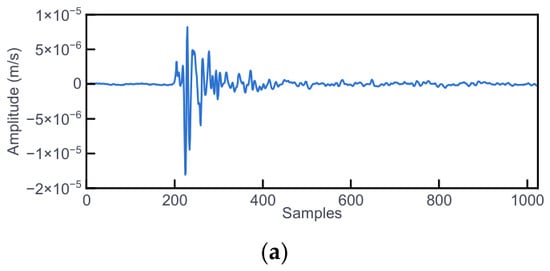
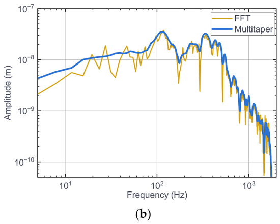
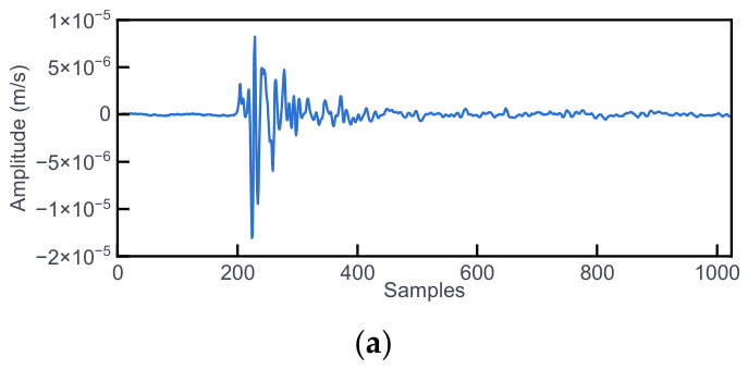
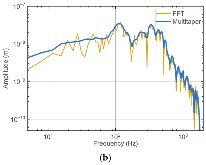
When the multitaper spectral algorithm is used, instead of averaging the data in segments, a set of windows is added to the same segment of data for FFT weighted averaging, and the obtained spectrum is superior to the WOSA or lag-window spectral techniques; in particular, the resolution of the spectrum is greatly improved. Figure 1 illustrates a comparative spectral analysis of a representative microseismic signal using both the standard FFT and the multitaper method. While the FFT-derived spectrum exhibits significant fluctuations and noise-induced artifacts, the multitaper estimate provides a markedly more stable and smoother spectral envelope. This enhanced stability is achieved by applying a set of orthogonal Slepian sequences as windows, which significantly suppresses spectral leakage and improves frequency resolution. Such precision is vital for the subsequent extraction of Q values from short-duration waves.
Figure 1.
(a) The microseismic signal and (b) its corresponding spectra estimated using the FFT and multitaper methods. NW = 4 and K = 5 were used for the multitaper estimate.
3. Data and Processing
3.1. Project Background
3.1.1. Project 1: Hanjiang-to-Weihe River Diversion Project (HRD)
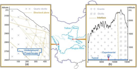
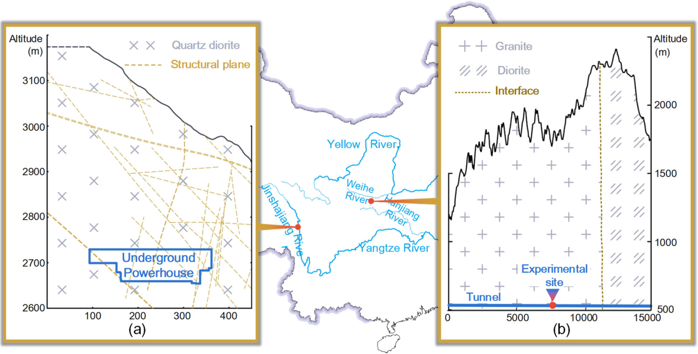
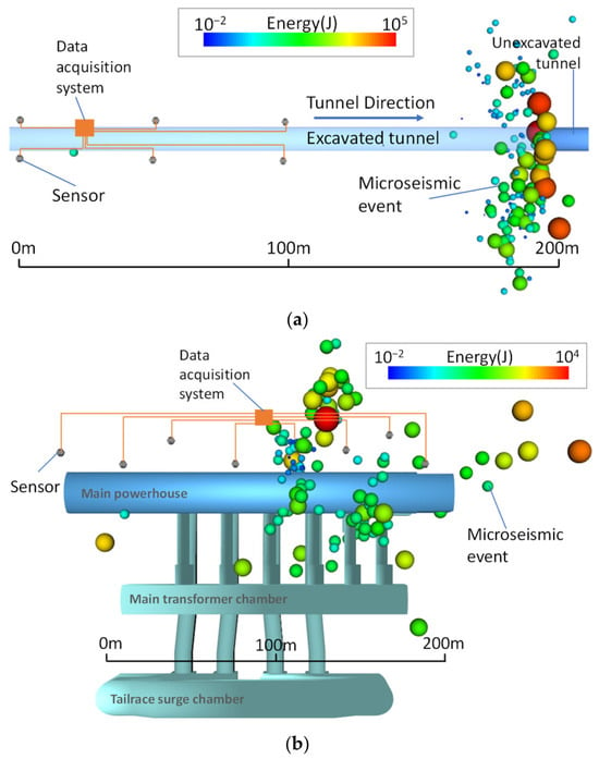
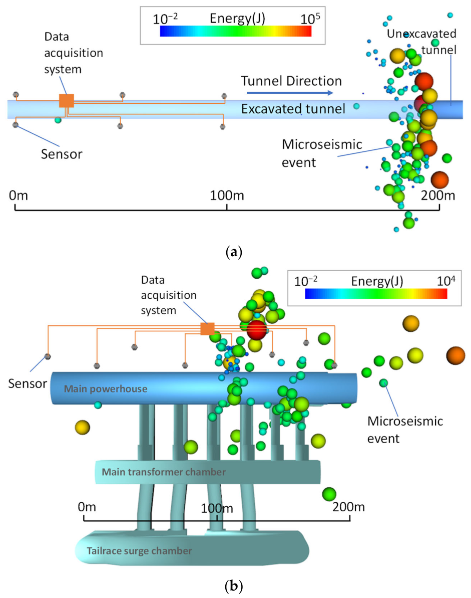
The Hanjiang-to-Weihe River Diversion Project (HRD) is located in Shaanxi Province, China. The Qinling water conveyance tunnel, a key component of the project, is 81.78 km long and has a maximum burial depth of approximately 2012 m, resulting in high geostress and elevated temperature conditions during construction [31,32]. The monitored region is a 40 m long section of Qinling Tunnel No. 4, buried at approximately 1250 m and dominated by granite (see Figure 2b). This section is representative of a deeply buried hard-rock tunnel. To support rockburst risk monitoring and construction safety assessment, a microseismic monitoring system comprising six single-component sensors arranged in three rows on both sides of the tunnel was installed, as shown in Figure 3a.
Figure 2.
Geographic location and geological conditions of the study sites. (a) The YHS test site is located in quartz diorite. (b) The HRD project area is characterized by granite and diorite lithologies, and the test site is located within the granite unit.
Figure 3.
Layout of the microseismic monitoring system for (a) HRD and (b) YHS. The gray dots in the figure represent the sensors deployed on-site, while the spheres of varying sizes and colors denote microseismic events and their magnitudes.
According to the site-specific parameters reported for the monitored HRD section [32], the P-wave velocity of the rock mass is vp = 5430 m/s, and the Poisson’s ratio is ν = 0.18. According to the relationship [33]:
the S-wave velocity can be calculated as vs = 3393 m/s.
3.1.2. Project 2: Yebatan Hydropower Station (YHS)
The Yebatan Hydropower Station (YHS) is located in the upper reaches of the Jinsha River, at the boundary between Sichuan Province and Tibet. The project includes an underground powerhouse, a concrete hyperbolic dam, and a flood dissipation system. The underground powerhouse comprises three main caverns: the main powerhouse, the main transformer chamber, and the tailrace surge chamber, together with associated auxiliary structures. The test site is located in quartz diorite. According to the geological survey, the underground powerhouse is buried at a vertical depth of 252–420 m, and the rock mass integrity is reduced by the presence of structural planes (see Figure 2a). During construction, local rock instability, including spalling and collapse, was observed. To monitor rock mass damage during excavation and support construction safety assessment, a microseismic monitoring system comprising eight single-component sensors was installed upstream of the main powerhouse, as shown in Figure 3b. The P-wave velocity of the rock mass in the study area is vp = 5002 m/s, and the Poisson’s ratio is ν = 0.24, giving an S-wave velocity of vs = 2926 m/s.
The sensors in both projects were tightly coupled with the rock mass through borehole grouting installation to improve waveform quality. Velocity sensors were used in both projects, with an effective frequency response range of 10~1000 Hz, and the sampling frequency of the system was 4000 Hz. The source location procedure was implemented using the Newton iterative method [34], while the seismic energy was calculated using a velocity spectrum integration approach based on the Brune source model (see Section 8.2 of Mendecki [35]).
A summary of the project conditions and monitoring system configurations for the two field cases is provided in Table 1.
Table 1.
Summary of the two engineering projects and monitoring systems.
The recorded data used in this study were obtained from the microseismic monitoring networks described above rather than from a single sensor. For each detected microseismic event, waveforms recorded by multiple sensors were used for event location and subsequent attenuation analysis. The source-to-sensor distances obtained from the monitoring networks were then used in the RAM and SRM calculations.
3.2. Window Selection
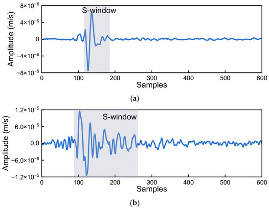
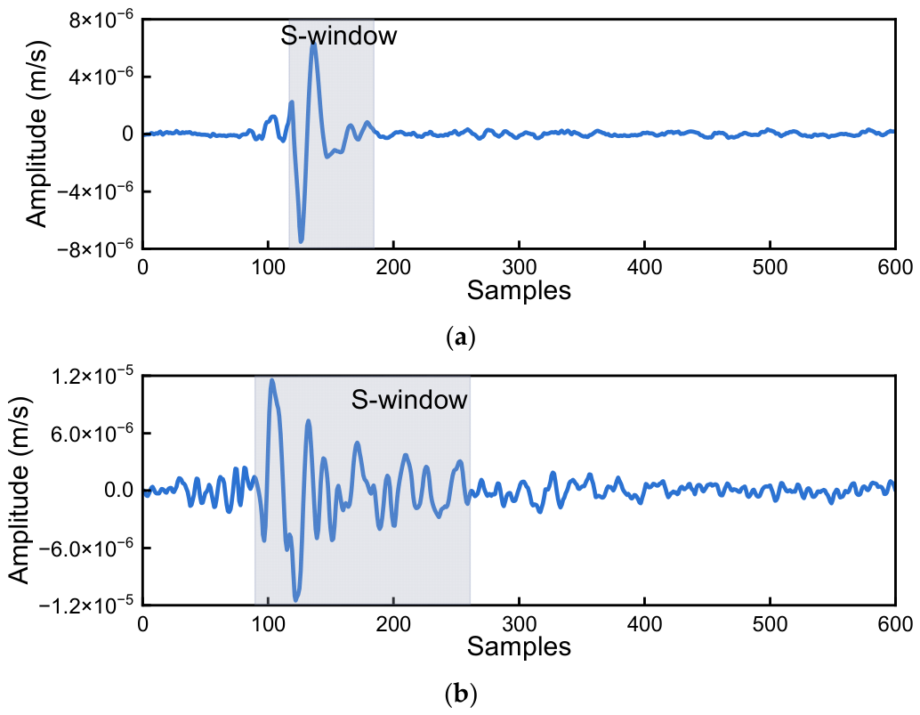
The “S-window” refers to the data window that contains the direct S-wave, and it is also the data segment directly used for attenuation calculation. The “S-window” generally ranges from the arrival of the S-wave to its termination. The arrival of the S-wave is usually relatively easy to identify, and a variety of methods have been developed for this purpose. In the absence of noise interference, the termination position of the S-wave can be set as far as possible from its arrival time, which ensures that all S-wave signals are included in the “S-window”. However, practical engineering scenarios are invariably subject to various types of noise interference. To mitigate such interference, the “S-window” needs to be as short as possible to eliminate the impact of noise signals on the calculation. Therefore, an appropriately sized “S-window” should contain most of the S-wave information while avoiding the noise segment to the greatest extent possible. Figure 4 displays the S-windows of a typical signal from the HRD and the YHS. It can be observed that the S-window of the HRD is shorter, whereas that of the YHS is longer.
Figure 4.
Schematic diagrams of the S-window of (a) the HRD and (b) the YHS.
To achieve consistent frequency resolution of Q in calculation, the lengths of the “S-windows” selected within the same project must be uniform.
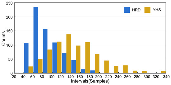
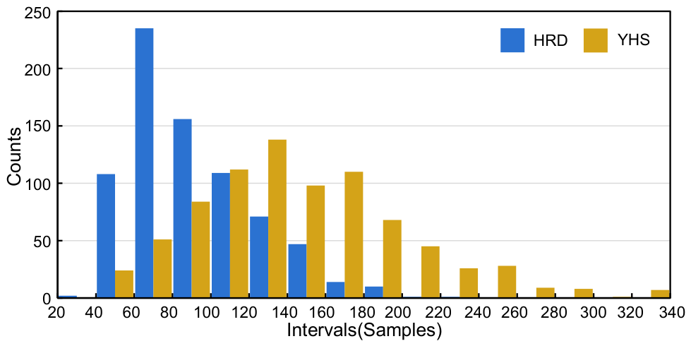
Based on the above principles, the S-window lengths of the HRD and YHS were statistically analyzed, and their distributions are shown in Figure 5. The results show that the S-window lengths of the microseismic data of the HRD are shorter and more concentrated overall, while the S-window lengths of the YHS are longer and more dispersed overall, which is related to the geological conditions and environmental noise. A higher rock mass integrity combined with lower background noise results in microseismic waveforms that are more impulsive and concentrated within the time domain.
Figure 5.
S-window length distribution interval statistics for the HRD and YHS.
Finally, the statistical average of 917 waveforms in the HRD yielded an S-window length of 92 samples; therefore, 100 samples were used for calculation convenience. For the YHS underground powerhouse, the statistical average of 831 waveforms yielded an S-window length of 148 samples; therefore, 150 samples were used. At the sampling frequency of 4000 Hz, these window lengths correspond to frequency resolutions of 40 Hz for the HRD and 26.7 Hz for the YHS, respectively.
3.3. Processing Workflow
According to the foregoing, there are two major steps in calculating the Q value: estimating the S-wave spectrum and calculating the Q value. The method of calculating the Q value is introduced in Section 2; when calculating the S-wave spectrum, the noise spectrum also requires attention. The steps for calculating the Q value are as follows.
Before spectral estimation and Q-value inversion, a waveform-level quality-control procedure was applied to reduce the influence of background noise. The P- and S-wave arrivals were manually picked from each waveform. For each triggered waveform, the S-wave signal window was extracted from two samples before the manually picked S-wave arrival. The pre-event noise window was selected before the manually picked P-wave arrival and ended 10 samples before the P-wave arrival to avoid contamination by the signal onset. The signal-to-noise ratio (SNR) was calculated from the average signal and noise energies as follows:
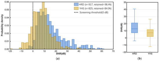
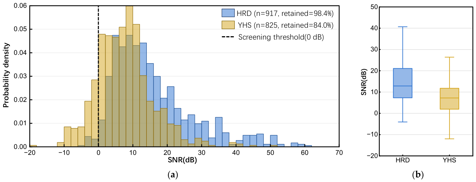
where and denote the average energies of the S-wave signal window and the pre-event noise window, respectively. Waveforms with SNR lower than 0 dB were regarded as strongly affected by noise and were excluded from the attenuation inversion. To make the data-selection procedure more transparent, the SNR distributions of the HRD and YHS datasets are summarized in Figure 6. The results show that 902 of 917 HRD waveforms (98.4%) and 693 of 825 YHS waveforms (84.0%) satisfied the SNR criterion. For the remaining valid waveforms, the spectra of the S-wave window and the pre-event noise window were calculated separately, and the observed spectrum used for Q estimation was obtained after noise-spectrum correction.
Figure 6.
SNR distributions of the waveforms used in this study. (a) Probability density distributions of SNR for the HRD and YHS datasets. (b) Boxplot summary of SNR values for the two projects. The dashed line indicates the waveform screening threshold of 0 dB.
After this quality-control procedure, the Q-value calculation was performed using the following steps:
- (1)
- Calculate the length of the “S-window” for each project and obtain an average window length L.
- (2)
- Extract a noise segment with a length of L before the P-wave arrival.
- (3)
- Calculate the frequency spectrum X(f) of the S-window and the frequency spectrum N(f) of the noise segment separately using the multitaper spectrum algorithm.
- (4)
- Subtract the noise spectrum N(f) from the frequency spectrum X(f) corresponding to the “S-window” to obtain the observed spectrum S(f).
- (5)
- In actual signal records, velocity spectra and acceleration spectra are generally used. For the convenience of calculation, convert the observed spectrum into a displacement spectrum.
- (6)
- Calculate the Q value using the RAM/SRM described in Section 2.
In the Q-value calculation using RAM, the objective function is the total residual defined in Equations (5) and (6). At each frequency point, the optimal Q value is determined by minimizing this residual. Because the RAM objective function is nonlinear with respect to Q, the differential evolution (DE) algorithm is employed for numerical minimization. DE is a population-based stochastic optimization algorithm that generates trial solutions through scaled differences between candidate parameter vectors and retains solutions with lower objective-function values [36]. In the SRM calculation, least-squares linear regression is used to estimate b(f) at each frequency point according to Equation (8), and the corresponding Q value is then calculated using Equation (9).
4. Results
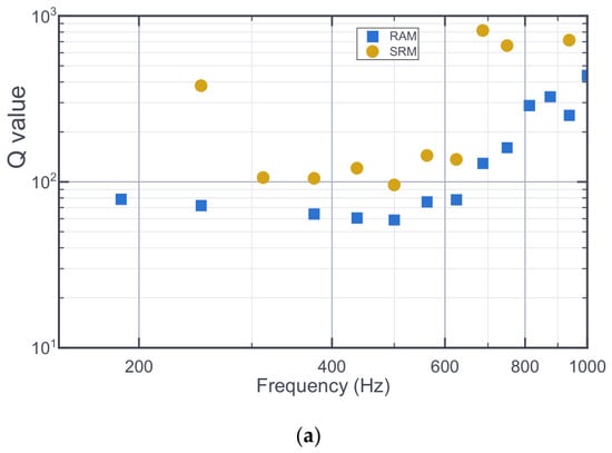
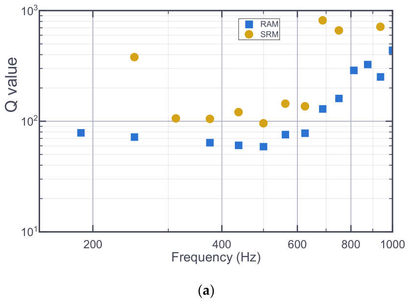
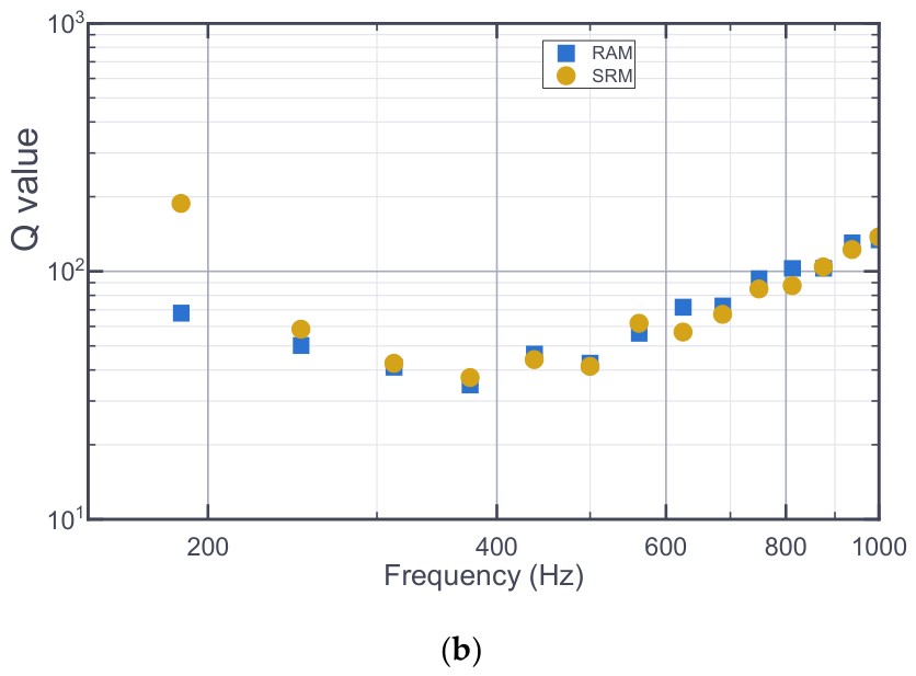
For the convenience of comparative analysis, calculations were also performed based on the original method [21,24,37]. The calculation results are presented in Figure 7. Although the Q factor generally exhibits a non-monotonic trend—initially decreasing before rising with frequency—this pattern remains indistinct in the unoptimized results. In the low-frequency range (f < 500 Hz), the Q values show high discreteness. Particularly in the HRD Project, the variation trend of Q with frequency is not clear. The ambiguous relationship between Q and frequency—specifically whether Q remains constant or attenuates—precludes the use of a unified mathematical model for these results. The frequency resolution of the Q value is 62.5 Hz, which is relatively low.
Figure 7.
Calculation results of (a) HRD and (b) YHS before optimization using the RAM and the SRM, respectively. The blue circle is the result of a calculation using the original RAM. The tan square is the result of the calculation using the original SRM.
Based on the calculation results of the two methods shown in the figure, it can be seen that the SRM results represented by the brown dots are more unstable than the RAM results represented by the blue dots. This indicates that directly applying the Atkinson method and the spectral ratio method to engineering microseismic data entails considerable problems.
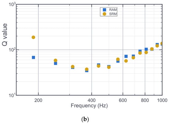
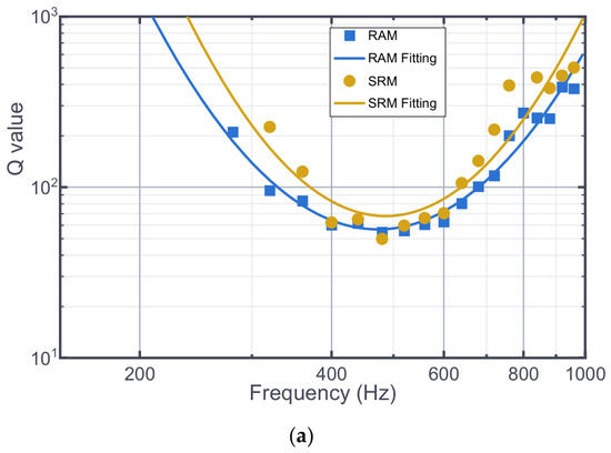
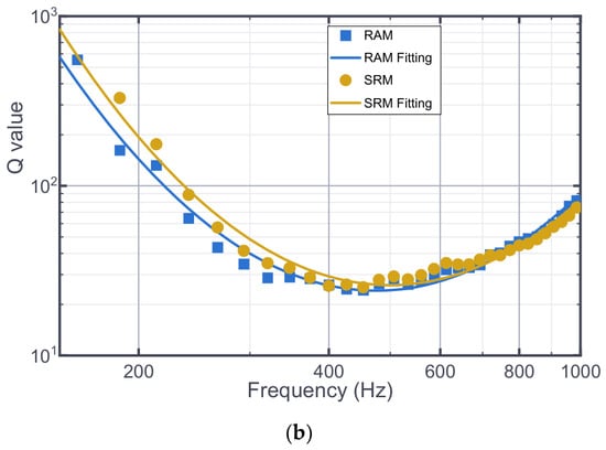
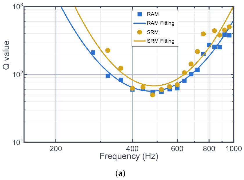
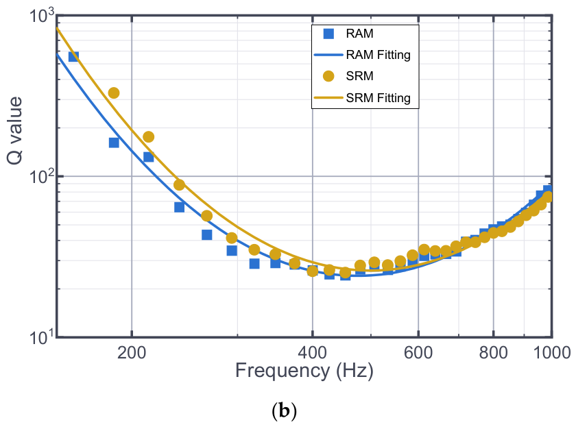
The attenuation Q values of the two projects were calculated based on the optimized Atkinson method and spectral ratio method, and the calculation results are presented in Figure 8. Overall, all the calculation results exhibit distinct regularity. A strong frequency dependence of the Q value is observed in all cases, with the Q value showing a trend of decreasing first and then increasing as the frequency rises. Compared with the calculation results obtained before optimization, the results yield a more consistent and stable distribution pattern. The frequency resolution of the Q value reaches 40 Hz (for HRD) and 26.7 Hz (for YHS), respectively, representing a substantial improvement.
Figure 8.
Calculation results of the optimized (a) HRD and (b) YHS using the RAM and the SRM. The blue square is the result of a calculation using the optimized RAM, and the blue curve is its fitted curve. The tan circle is the result of the calculation using the optimized SRM, and the tan curve is its fitted curve.
Visual analysis shows that the calculated results approximate a parabolic shape in the logarithmic coordinate system. To quantitatively describe the Q value, the following expression is adopted for fitting:
The calculation and fitting results of the two methods in the two projects are shown in Figure 8, and the fitted expressions are shown in Table 2.
Table 2.
Attenuation Calculation Fitting Results by the RAM and SRM.
Next, the attenuation results for the same project calculated by the two methods were compared. For the HRD, the minimum Q values obtained by the two methods were 55 (RAM) and 50 (SRM), respectively. After fitting, the minimum Q value calculated by the Atkinson method was Qmin ≈ 56.65, with the axis of symmetry at f = 473.13 and the quadratic coefficient a = 9.95. In contrast, the fitting results of the spectral ratio method showed Qmin ≈ 67.78, with the axis of symmetry at f = 486.00 and the quadratic coefficient a = 12.09. These parameters are very similar. The coefficient of determination (goodness of fit) of the fitting based on the RAM results was 0.95, while that based on the SRM results was 0.87, indicating a high correlation between the numerical values and the curve model.
For the RAM results, the minimum Q value for the HRD is Qmin = 50 and that for the YHS is Qmin = 24. After curve fitting, the minimum Q value of the HRD is Q’min = 56.65 with a quadratic term coefficient a = 9.95 (the coefficient a reflects the growth rate or opening size of the parabola; the larger a is, the faster the curve growth), and the minimum Q value of the YHS is Qmin = 24.10 with a quadratic term coefficient a = 5.49. The above calculation results and curve fitting results show that the Q value of the HRD is higher than that of the YHS. The same conclusion can be obtained for the calculation results of the SRM.
The higher Q value of the HRD than that of the YHS indicates that the microseismic wave propagation attenuation in the HRD is less than that in the YHS. This is due to the high ground stress and intact rock mass in the HRD and the lower ground stress and more fragmented rock mass in the YHS. This is consistent with the understanding that Q values are closely related to geological conditions, indicating that Q values can reflect geological information and verifying the reasonableness of the calculation results.
5. Discussion
Reliable estimation of microseismic attenuation has direct implications for engineering decision-making. First, improved Q estimates provide a more stable basis for characterizing attenuation behavior and comparing propagation conditions among engineering rock masses. Second, because attenuation is closely linked to rock mass integrity and heterogeneity, spatial or temporal variations in Q can serve as indicators of damage accumulation and stress redistribution during excavation. Although the present analysis is based on two specific engineering projects with distinct geological settings, the proposed workflow is not restricted to these sites. Its broader applicability lies in the processing strategy for short-duration, high-frequency, and noise-contaminated microseismic body waves, including fixed-length S-window selection, multitaper spectral estimation, and frequency-dependent Q inversion using RAM and SRM. Therefore, the method can be applied to other geotechnical engineering projects where microseismic events are recorded by a sensor network and reliable source-to-sensor distances are available. However, the absolute Q values and fitted attenuation parameters should be interpreted as site-dependent quantities and should be re-evaluated according to local lithology, fracture development, in situ stress conditions, sensor geometry, and noise level. The following sections further evaluate the performance of the proposed methodologies, discuss the underlying physical mechanisms, and explore the practical implications alongside the inherent limitations of this study.
5.1. The Comparison of RAM and SRM
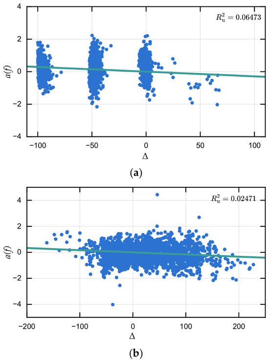
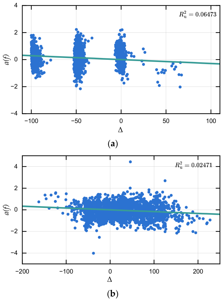
Figure 8 indicates that the Q estimates for the YHS have higher frequency resolution than those for the HRD, primarily because the YHS waveforms have longer durations (Figure 4). Nevertheless, the variation pattern of Q with frequency is preserved in both projects. Table 3 shows that the determination coefficients obtained for the YHS are higher than those for the HRD when the same method is applied, indicating greater overall stability of the fitted Q-frequency relationships for the YHS dataset. This difference may be associated with both waveform duration and sensor-source geometry; at the HRD site, the sensors are mainly distributed on one side of the sources, which may provide less favorable ray-path coverage. Figure 9 illustrates the SRM fitting process for b(f) = πf/[vQ(f)] at one selected frequency point for each project. The values displayed in the two panels quantify the zero-intercept linear fits only at the shown frequency points and are not used as a project-wide comparison of inversion performance.
Table 3.
Attenuation Model Parameters Derived from RAM and SRM.
Figure 9.
SRM fitting process for b(f) at one selected frequency point in (a) the HRD and (b) the YHS. The horizontal axis Δ denotes the differential hypocentral distance, and the vertical axis a(f), calculated using Equation (9), denotes the distance-corrected spectral ratio. The scattered points are calculated from recorded microseismic events, and the solid line represents the zero-intercept linear fit prescribed by Equation (8). The displayed values are the uncentered coefficients of determination for the zero-intercept fits.
It can also be seen in Table 3 that the determination coefficients of the RAM results are all higher than those of the SRM. The difference between the computed results of these two methods in YHS is not significant, but the difference in HRD is larger. In Figure 8a, it can be seen that the SRM results are generally more scattered, especially at low and high frequencies. The above results indicate that if the position of sensors relative to the seismic source is more dispersed, the difference between the results calculated by RAM and SRM is not significant. When the position of sensors relative to the source is less favorable, the results of RAM are better than those of SRM, which indicates that SRM requires higher quality data and is less stable than RAM.
Based on the above comparison, the key methodological differences and application-related insights of RAM and SRM are summarized in Table 4.
Table 4.
Comparison between the RAM and SRM approaches in this study.
5.2. Discussion on Attenuation Law
Combining the results of the above analyses, the results of the two projects calculated using the two methods show consistency in general, i.e., the Q value is closely dependent on frequency and first decreases and then increases with increasing frequency. This trend is in high agreement with that exhibited by the standard linear solid model [38]. This suggests that the reason for this pattern may be related to intrinsic absorption, although it is generally accepted that intrinsic absorption, which can be characterized by the generalized standard linear solid model, is frequency-independent. The more likely reason is that the attenuation is mainly caused by scattering, which closely agrees with the corresponding trend for inhomogeneous media derived by Wu [39] and Sato [40,41] on the basis of Born’s approximation theory. As early as 1980, Aki [42] conjectured that the Q value has a valley at some frequency. Sato built his theoretical model based on Aki’s conjecture. The results calculated by Fehler et al. [43] showed the same pattern of the Q value being closely dependent on frequency, first decreasing and then increasing with increasing frequency, while a lower-resolution Q value trend was obtained by his calculations. This may be because the finite length of the coda wave at low frequencies prevented him from obtaining a reliable result, which thus prevented him from capturing the variation in the Q value over a wider bandwidth and led him to believe that the variation in the Q value was only weakly frequency dependent. In addition to the above attenuation pattern caused by intrinsic or scattering attenuation, another possible explanation is noise. Assuming that the noise is uniformly distributed throughout the frequency band, the weight of the noise in the microseismic signal becomes larger with increasing frequency. In the low frequency band, the proportion of the noise relative to the microseismic signal is negligible, and as the frequency increases the microseismic wave attenuates more and more, and the result is manifested as a Q value that becomes smaller with frequency. In the higher frequency bands, the effect of noise becomes progressively more significant. Homogeneous noise then exhibits a decrease in apparent attenuation, which manifests itself as an increase in the Q value. Overall, although the above trend of a frequency-dependent Q value with a valley has been found and can be supported theoretically, the evidence in support of this trend is not sufficient, and more observational evidence is needed to verify it.
5.3. Engineering Implications and Limitations
To facilitate practical application, the evolution of the Q value provides a promising conceptual framework for assessing engineering safety. As micro-fractures accumulate under geostress, the intensification of seismic wave scattering may lead to a detectable reduction in the quality factor. However, whether such a reduction can serve as a definitive precursor for rock mass instability—such as rockbursts or collapses—remains an open question that requires further systematic research. Establishing robust early-warning criteria will depend on further enhancing the inversion accuracy and numerical reliability of Q estimation across a wider range of geological conditions.
Despite the improvements achieved by the optimized framework, a primary inherent limitation of the current study lies in the sensitivity to source location and distance uncertainty. The hypocentral distance r is a fundamental input for both RAM and SRM, serving as the basis for calculating geometric spreading and path-dependent attenuation. Consequently, the accuracy of the Q factor estimation is intrinsically coupled with the precision of microseismic localization. Inherent uncertainties in source coordinates can propagate directly into the attenuation inversion, potentially introducing systematic bias into the Q(f) profile. A rigorous quantitative assessment of how localization errors—stemming from velocity model inaccuracies or arrival-time picking uncertainties—influence the stability and resolution of Q values remains a critical subject for future sensitivity analyses. Because the monitoring systems used single-component sensors, the reconstructed S-wave amplitudes may still be affected by sensor orientation and radiation-pattern effects; therefore, the derived Q values should be interpreted as statistically averaged attenuation parameters over many source-sensor paths rather than as fully vector-resolved wavefield measurements.
Future studies should focus on refining attenuation models to account for anisotropy and on bridging the gap between geophysical parameters and real-time engineering decision-making through long-term temporal monitoring.
6. Conclusions
This study presents an optimized framework for estimating frequency-dependent attenuation of microseismic body waves that is specifically tailored to the characteristics of geotechnical engineering data. By adopting fixed-length S-wave windows and replacing conventional lag-window spectral estimation with the multitaper method, both the frequency resolution and numerical stability of Q-value estimation are significantly improved. Applications to two large-scale engineering projects demonstrate that the optimized regression analysis and spectral ratio methods yield consistent and physically meaningful results, with the regression analysis method showing superior robustness under less favorable sensor geometries.
The obtained Q values exhibit a clear frequency-dependent pattern, decreasing at low frequencies and increasing at higher frequencies, and their relative magnitudes correlate well with rock mass integrity and stress conditions at the project sites. These findings confirm that microseismic attenuation parameters can serve as effective indicators of engineering geological conditions. Overall, the proposed methodology provides a reliable basis for attenuation-aware microseismic analysis, contributing to more accurate source parameter estimation, improved interpretation of rock mass damage, and enhanced early warning capabilities for underground engineering hazards.
Author Contributions
Conceptualization, X.Z.; methodology, X.Z.; software, B.C.; validation, B.C.; formal analysis, B.C.; investigation, X.Z.; resources, B.C.; data curation, X.Z.; writing—original draft preparation, X.Z.; writing—review and editing, B.C.; visualization, X.Z.; supervision, B.C.; project administration, B.C.; funding acquisition, X.Z. and B.C. All authors have read and agreed to the published version of the manuscript.
Funding
This research was funded by the National Natural Science Foundation of China (grant no. 52509157), and the Deep Earth Probe and Mineral Resources Exploration-National Science and Technology Major Project (grant no. 2025ZD1011302).
Data Availability Statement
All the datasets obtained and discussed in this study are available at https://doi.org/10.5281/zenodo.8249065.
Acknowledgments
The Hanjiang-to-Weihe River Valley Water Diversion Project Construction Co., Ltd., and Chengdu Engineering Corporation Limited provided invaluable support and assistance during field monitoring and data acquisition.
Conflicts of Interest
The authors declare no conflicts of interest.
References
- Chen, B.-R.; Feng, X.-T.; Li, Q.-P.; Luo, R.-Z.; Li, S. Rock Burst Intensity Classification Based on the Radiated Energy with Damage Intensity at Jinping II Hydropower Station, China. Rock Mech. Rock Eng. 2015, 48, 289–303. [Google Scholar] [CrossRef] [Scilit]
- Dai, F.; Li, B.; Xu, N.; Fan, Y.; Zhang, C. Deformation Forecasting and Stability Analysis of Large-Scale Underground Powerhouse Caverns from Microseismic Monitoring. Int. J. Rock Mech. Min. Sci. 2016, 86, 269–281. [Google Scholar] [CrossRef] [Scilit]
- Zhao, J.-S.; Jiang, Q.; Lu, J.-F.; Chen, B.-R.; Pei, S.-F.; Wang, Z.-L. Rock Fracturing Observation Based on Microseismic Monitoring and Borehole Imaging: In Situ Investigation in a Large Underground Cavern under High Geostress. Tunn. Undergr. Space Technol. 2022, 126, 104549. [Google Scholar] [CrossRef] [Scilit]
- Castro, R.R.; Mendoza-Camberos, A.; Pérez-Vertti, A. Radiated Seismic Energy of Earthquakes in the South–Central Region of the Gulf of California, Mexico. Geophys. J. Int. 2018, 214, 990–1003. [Google Scholar] [CrossRef] [Scilit]
- Zhu, L.; Helmberger, D.V. Advancement in Source Estimation Techniques Using Broadband Regional Seismograms. Bull. Seismol. Soc. Am. 1996, 86, 1634–1641. [Google Scholar] [CrossRef] [Scilit]
- Pugh, D.J.; White, R.S. MTfit: A Bayesian Approach to Seismic Moment Tensor Inversion. Seismol. Res. Lett. 2018, 89, 1507–1513. [Google Scholar] [CrossRef] [Scilit]
- Santos, E.B.; Dantas, R.R.S.; Xavier, M.M., Jr.; Medeiros, W.E.; Santana, F.L.; Correa, M.A. Constant-Q Model Can Reproduce the Frequency-Dependent Dispersion of GPR Signals in Sedimentary Rocks. J. Appl. Geophys. 2025, 243, 105945. [Google Scholar] [CrossRef] [Scilit]
- Das, V.; Mukerji, T.; Mavko, G. Scale Effects of Velocity Dispersion and Attenuation (Q-1) in Layered Viscoelastic Medium. Geophysics 2019, 84, T147–T166. [Google Scholar] [CrossRef] [Scilit]
- Wang, Y. A Constant-Q Model for General Viscoelastic Media. Geophys. J. Int. 2019, 219, 1562–1567. [Google Scholar] [CrossRef] [Scilit]
- Hao, Q.; Tsvankin, I. Thomsen-Type Parameters and Attenuation Coefficients for Constant-Q Transverse Isotropy. Geophysics 2023, 88, C123–C134. [Google Scholar] [CrossRef] [Scilit]
- Li, H.; Liu, B.; Liu, X.; Al-Shuhail, A.A.; Mahmoud, S.M.H.; Chen, Y. Frequency-Independent Centroid Frequency Shift Method for Signal Attenuation Estimation. IEEE Trans. Geosci. Remote Sens. 2023, 61, 4504212. [Google Scholar] [CrossRef] [Scilit]
- Solomon, S.C.; Toksöz, M.N. Lateral Variation of Attenuation of P and S Waves beneath the United States. Bull. Seismol. Soc. Am. 1970, 60, 819–838. [Google Scholar] [CrossRef]
- Chen, X.; Zong, Z.; Yang, Y.; Zeng, Y. Frequency-Dependent Nonlinear AVO Inversion for Q-Factors in Viscoelastic Media. IEEE Trans. Geosci. Remote Sens. 2023, 61, 5900817. [Google Scholar] [CrossRef] [Scilit]
- Xiao, P.; Mao, H.; Qian, B.; Li, B.; Yang, X.; Xu, N. Stability Analysis of Surrounding Rock Mass in Underground Powerhouse Considering Damage Effect of Microfractures. J. Rock Mech. Geotech. Eng. 2022, 14, 1115–1130. [Google Scholar] [CrossRef] [Scilit]
- Atkinson, G.M.; Mereu, R.F. The Shape of Ground Motion Attenuation Curves in Southeastern Canada. Bull. Seismol. Soc. Am. 1992, 82, 2014–2031. [Google Scholar] [CrossRef] [Scilit]
- Kkallas, C.; Papazachos, C.B.; Margaris, B.N.; Boore, D.; Ventouzi, C.; Skarlatoudis, A. Stochastic Strong Ground Motion Simulation of the Southern Aegean Sea Benioff Zone Intermediate-Depth Earthquakes. Bull. Seismol. Soc. Am. 2018, 108, 946–965. [Google Scholar] [CrossRef] [Scilit]
- Ren, Y.; Zhou, Y.; Wang, H.; Wen, R. Source Characteristics, Site Effects, and Path Attenuation from Spectral Analysis of Strong-Motion Recordings in the 2016 Kaikoura Earthquake Sequence. Bull. Seismol. Soc. Am. 2018, 108, 1757–1773. [Google Scholar] [CrossRef] [Scilit]
- Feustal, A.J. Seismic Attenuation in Underground Mines: Measurement Techniques and Applications to Site Characterization. Doctoral Dissertation, Queen’s University, Kingston, ON, Canada, 1995. [Google Scholar]
- Cichowicz, A.; Green, R.W.E. Changes in the Early Part of the Seismic Coda Due to Localized Scatterers: The Estimation of Q in a Stope Environment. Pure Appl. Geophys. 1989, 129, 497–511. [Google Scholar] [CrossRef] [Scilit]
- Feustel, A.J.; Young, R.P. Qβ Estimates from Spectral Ratios and Multiple Lapse Time Window Analysis: Results from an Underground Research Laboratory in Granite. Geophys. Res. Lett. 1994, 21, 1503–1506. [Google Scholar] [CrossRef] [Scilit]
- Zhu, X.; Chen, B.; Cao, D.; Wang, X.; Wang, Q. Study on the Calculation of Attenuation Quality Factor Q-Value in Microseismic Monitoring: Results from Two Rock Engineering Cases. Adv. Transdiscipl. Eng. 2022, 31, 814–822. [Google Scholar] [CrossRef] [Scilit]
- Chun, K.-Y.; West, G.F.; Kokoski, R.J.; Samson, C. A Novel Technique for Measuring Lg Attenuation—Results from Eastern Canada between 1 to 10 Hz. Bull. Seismol. Soc. Am. 1987, 77, 398–419. [Google Scholar] [CrossRef] [Scilit]
- Chung, T.W.; Park, Y.K.; Kang, I.B.; Lee, K. Crustal QLg−1 in South Korea Using the Source Pair/Receiver Pair Method. Bull. Seismol. Soc. Am. 2005, 95, 512–520. [Google Scholar] [CrossRef] [Scilit]
- Zhu, X.; Chen, Y. An Inversion of Site Response and Lg Attenuation Using Lg Waveform. Acta Seismol. Sin. 2007, 20, 605–616. [Google Scholar] [CrossRef] [Scilit]
- Chael, E.P. Spectral Scaling of Earthquakes in the Miramichi Region of New Brunswick. Bull. Seismol. Soc. Am. 1987, 77, 347–365. [Google Scholar] [CrossRef] [Scilit]
- Konno, K.; Ohmachi, T. Ground-Motion Characteristics Estimated from Spectral Ratio between Horizontal and Vertical Components of Microtremor. Bull. Seismol. Soc. Am. 1998, 88, 228–241. [Google Scholar] [CrossRef] [Scilit]
- Thomson, D.J. Spectrum Estimation and Harmonic Analysis. Proc. IEEE 1982, 70, 1055–1096. [Google Scholar] [CrossRef] [Scilit]
- Bronez, T.P. On the Performance Advantage of Multitaper Spectral Analysis. IEEE Trans. Signal Process. 1992, 40, 2941–2946. [Google Scholar] [CrossRef] [Scilit]
- Wang, Y. Quantifying the Effectiveness of Stabilized Inverse Q Filtering. Geophysics 2003, 68, 337–345. [Google Scholar] [CrossRef] [Scilit]
- Slepian, D. Prolate Spheroidal Wave Functions, Fourier Analysis, and Uncertainty—V: The Discrete Case. Bell Syst. Tech. J. 1978, 57, 1371–1430. [Google Scholar] [CrossRef] [Scilit]
- Liu, F.; Tang, C.; Ma, T.; Tang, L. Characterizing Rockbursts Along a Structural Plane in a Tunnel of the Hanjiang-to-Weihe River Diversion Project by Microseismic Monitoring. Rock Mech. Rock Eng. 2019, 52, 1835–1856. [Google Scholar] [CrossRef] [Scilit]
- Liu, F.; Zhang, Y.; Ma, T.; Liang, C. Interpretation of Generation Process and Precursors of Successive Rockbursts in a Deep Hard-Rock Water Conveyance Tunnel by Microseismic Monitoring. J. Appl. Geophys. 2025, 243, 105973. [Google Scholar] [CrossRef] [Scilit]
- Tatham, R.H. Vp/Vs and Lithology. Geophysics 1982, 47, 336–344. [Google Scholar] [CrossRef] [Scilit]
- Li, Q.P.; Chen, B.R. Research on Micro-Seismic Source Location During Linear Excavation Process of Deep Tunnel. In Proceedings of the ISRM SINOROCK 2013, Shanghai, China, 18–20 June 2013. [Google Scholar]
- Mendecki, A.J. Seismic Monitoring in Mines; Chapman & Hall: London, UK, 1997. [Google Scholar]
- Storn, R.; Price, K. Differential Evolution—A Simple and Efficient Heuristic for Global Optimization over Continuous Spaces. J. Glob. Optim. 1997, 11, 341–359. [Google Scholar] [CrossRef] [Scilit]
- Atkinson, G.M. Attenuation and Source Parameters of Earthquakes in the Cascadia Region. Bull. Seismol. Soc. Am. 1995, 85, 1327–1342. [Google Scholar] [CrossRef] [Scilit]
- Ben-Menahem, A.; Singh, S.J. Seismic Waves and Sources; Springer: New York, NY, USA, 1981. [Google Scholar]
- Wu, R.-S. Attenuation of Short Period Seismic Waves Due to Scattering. Geophys. Res. Lett. 1982, 9, 9–12. [Google Scholar] [CrossRef] [Scilit]
- Sato, H. Attenuation of S Waves in the Lithosphere Due to Scattering by Its Random Velocity Structure. J. Geophys. Res. 1982, 87, 7779–7785. [Google Scholar] [CrossRef] [Scilit]
- Sato, H. Unified Approach to Amplitude Attenuation and Coda Excitation in the Randomly Inhomogeneous Lithosphere. Pure Appl. Geophys. 1990, 132, 93–121. [Google Scholar] [CrossRef] [Scilit]
- Aki, K. Scattering and Attenuation of Shear Waves in the Lithosphere. J. Geophys. Res. Solid Earth 1980, 85, 6496–6504. [Google Scholar] [CrossRef] [Scilit]
- Fehler, M.; Roberts, P.; Fairbanks, T. A Temporal Change in Coda Wave Attenuation Observed during an Eruption of Mount St. Helens. J. Geophys. Res. 1988, 93, 4367–4373. [Google Scholar] [CrossRef] [Scilit]

Disclaimer/Publisher’s Note: The statements, opinions and data contained in all publications are solely those of the individual author(s) and contributor(s) and not of MDPI and/or the editor(s). MDPI and/or the editor(s) disclaim responsibility for any injury to people or property resulting from any ideas, methods, instructions or products referred to in the content. |
© 2026 by the authors. Licensee MDPI, Basel, Switzerland. This article is an open access article distributed under the terms and conditions of the Creative Commons Attribution (CC BY) license.