


Abstract
Spontaneous potential (SP) logging remains a widely used method in well geophysics. However, its interpretation is often limited by simplified physical models and correction charts that do not fully account for the processes governing SP generation, particularly in shaly and heterogeneous formations. In this study, we develop a finite element-based algorithm for modeling SP responses in complex near-wellbore environments, with the aim of providing a more physically consistent framework for interpretation. The proposed algorithm is based on the numerical solution of the Poisson equation with electrochemical source terms, incorporating the cation transport number to describe diffusion–adsorption processes and allowing for smooth variations in formation resistivity, fluid properties, and shale content. The numerical implementation is validated against published analytical solutions, correction charts, and previous numerical studies, showing good agreement in both the shape and amplitude of modeled SP responses across a range of geological scenarios, including thin beds and invasion zones. Application to real data from a Southeast Asia gas field demonstrates that the approach provides reliable estimates of formation water salinity and the cation transport number, with results consistent with independent estimates. The proposed method offers a flexible tool for SP response modeling and may complement existing interpretation techniques, particularly when working with heterogeneous formations and limited legacy datasets.
1. Introduction
Despite its nearly century-long history, spontaneous potential (SP) logging remains a widely used method in well geophysics. It is commonly applied for lithological differentiation of well sections, identification of pay zones, and estimation of their shale content. However, in practice, the interpretation of SP data is often based on a number of simplifying assumptions. The primary toolkit for SP log analysis still consists of correction charts derived from equivalent electrical circuits and analytical solutions obtained for simplified models [1,2,3]. In some cases, these charts allow the effects of shoulder beds, heterogeneous resistivity distribution, and the presence of a mud filtrate invasion zone to be taken into account. However, this approach does not fully capture the physical and chemical processes responsible for the formation of SP responses [4], which may lead to unreliable interpretation results.
At the same time, more advanced approaches to well log interpretation have been developed that rely on the solution of forward and inverse problems. Several numerical techniques have been successfully applied to model the SP response, including the finite element method [5,6], the finite difference method [7,8], and the mode-matching method [9], among others. Despite improving interpretation quality over traditional correction charts, most of these approaches share a key limitation: they rely on the static potential approximation, which provides an incomplete description of SP generation [1]. In this approach, SP sources are represented by infinitely extended dipole layers positioned at the interfaces between the borehole and the adjacent formations. This oversimplifies the physical mechanisms behind the SP response. The static potential model applies strictly to clean sandstones and cannot reliably link formation petrophysical properties to the observed SP response. As a result, it may lead to incorrect interpretation of SP logs in shaly reservoirs.
A key aspect in the study of such formations is the proper characterization of shale-related parameters in the reservoir. The presence of clay minerals significantly affects not only the electrical resistivity of the reservoir rock but also its diffusion–adsorption activity, which controls the magnitude of the SP response [10]. The behavior of SP logs in shaly formations can be explained by incorporating shale content into the earth model via petrophysical relationships that link clay volume and type to the macroscopic electrochemical properties of the formations.
A major contribution to the development of this approach was made by the work [4], in which total ionic diffusion is treated as the combined effect of diffusion through the pore fluid and ion drift along the solid–water interface within the electrical double layer. The application of the coupled-flux formalism [11] and nonequilibrium thermodynamics made it possible to relate the magnitude of the diffusion–adsorption potential to porosity and the cation exchange capacity of the solid particles forming the rock matrix. This parameter reflects the amount of surface-exchangeable counterions per unit mass of porous material and depends both on the type of clay minerals present in the formation and on their concentration. The model was later extended to describe ion diffusion in media with arbitrary degrees of fluid saturation [12].
In [13], this approach was employed to develop an algorithm for inverting key reservoir petrophysical parameters, including formation water salinity, porosity, water saturation, cation exchange capacity, cementation exponent, and saturation exponent. However, the model’s complexity means that solving the inverse problem requires not only SP logs but also resistivity, density, neutron porosity, and gamma-ray data. The need for such extensive a priori information therefore limits the applicability of the method, particularly when interpreting incomplete legacy datasets.
Another key aspect in modeling and interpreting SP logs is how the spatial distribution of formation electrophysical properties is parameterized. A common approach, used in resistivity well log inversion of any dimensionality, is to represent properties as piecewise-constant zones. This makes both theoretical analysis and numerical modeling straightforward. In practice, each layer is usually described by just two radial blocks (annular zones): the invaded zone and the virgin formation. This parameterization can explain measured logging responses with sufficient accuracy for most practical purposes, as long as the formation models adequately represent the studied deposits. It remains the predominant method in SP data modeling [5,9,13,14,15].
Nevertheless, piecewise-constant parameterization of the radial property profile is not entirely natural. It was already recognized in the 1950s [16,17] that the variation in formation resistivity with distance from the borehole wall during mud filtrate invasion is not truly stepwise. In general, a hydrodynamically consistent representation involves a smooth radial variation in properties, since the profile is formed by gradual filtration of drilling mud into the reservoir with partial mixing as formation fluid is displaced. Radial resistivity profiles have been studied, and methods have been proposed to account for near-wellbore variations in a simplified manner during modeling and inversion of well log data [18,19].
This issue becomes particularly important when integrating results from different physical measurements. In such cases, approximating the radial resistivity profile with just two piecewise-constant zones may be insufficient, and additional subdivision into several steps is applied. Moreover, reconciling different measurement types requires a consistent parameterization of the formation across all analyzed methods. For modeling SP responses, this approach is employed in [8]. However, it should be noted that in that study, the influence of resistivity contrast in the near-wellbore region on the SP response is neglected for electrochemical sources and considered only for electrokinetic sources.
In summary, current techniques for interpreting SP logs do not fully exploit the potential of the method. A growing trend in petroleum geophysics is the reinterpretation of legacy well log data to identify hydrocarbon accumulations that may have been overlooked in mature fields. One of the key reasons for such oversights is the presence of shaly zones, which create complex near-wellbore environments. In this context, the limitations of conventional SP interpretation approaches become particularly evident. Meanwhile, SP data are abundantly available in legacy datasets and may represent the only source of information for estimating formation water salinity. The development of more advanced SP interpretation tools therefore provides an opportunity to extract more complete and reliable information about reservoir properties, even under conditions of limited data.
This paper presents a newly developed algorithm for modeling SP well logs in complex near-wellbore environments using the finite element method. The algorithm is implemented within the classical paradigm [1,3], which accounts for resistivity contrasts among the borehole, the invaded zone, the uninvaded formation, and surrounding rocks, controlling the amplitude and shape of the SP response. At the same time, it incorporates a physically grounded electrochemical source term expressed via the cation transport number directly into the FEM formulation, preserving the link between SP response and petrophysical properties. In contrast to conventional piecewise-constant models, the proposed approach introduces a smooth parameterization of radial and vertical variations in formation resistivity, formation water salinity, and cation transport number, enabling a more realistic representation of mud-filtrate invasion and heterogeneous formations. The accuracy of the algorithm is validated against solutions available in the open literature, and its applicability to real-world problems is demonstrated through simulations in a model of sediments from one of Southeast Asia’s natural gas fields.
2. Methodology
2.1. Geological Model and Physical Principles of Spontaneous Potential Generation
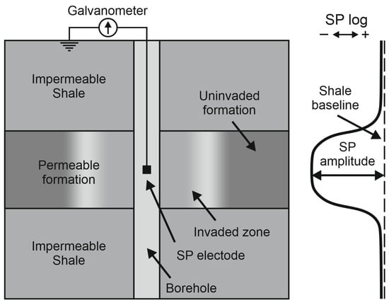
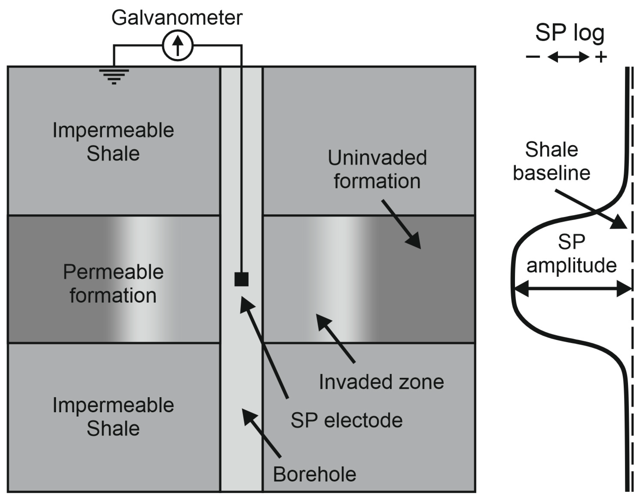
The problem is formulated for a geological model representing a vertical borehole that intersects a sequence of plane-parallel sedimentary formations with varying thickness and significant contrasts in electrical properties (Figure 1). During drilling, mud filtrate invades permeable reservoir formations, creating a near-wellbore zone with altered fluid saturation. In conventional well-logging practice, the radial structure of this region is commonly represented by a set of coaxial cylindrical zones, typically including the flushed zone and the transition or annulus zone. However, a hydrodynamically consistent description requires a smooth radial variation in properties, as the profile develops due to progressive filtrate invasion into the pore space and its partial mixing with the formation fluid during displacement.
Figure 1.
Schematic representation of SP generation in a geological medium with altered near-wellbore zones of permeable formations.
Spontaneous potentials arise from electromotive forces (EMFs) that develop at the boundaries between media with contrasting electrophysical properties. These forces drive ion motion in the pore fluid, leading to the generation of source currents that produce a potential distribution in the near-wellbore region. The total current in the medium is the sum of conduction and source currents. Applying the law of electric charge conservation leads to the Poisson equation:
where is the electrical conductivity of the medium, and is the scalar potential of the spontaneous polarization field, —volume current density of external sources.
The main contribution to arises from the electrochemical source caused by ionic diffusion between regions with different concentrations of dissolved salts. The effect of filtration and redox processes on the amplitude of spontaneous polarization potentials is much smaller and can usually be neglected [8,13,14,20,21].
By analogy with [13], the current density of the electrochemical source can be expressed as
where is the Hittorf transport number for cations, is Bolzman constant (J/K), is temperature (K), is the elementary charge (C), and is the electrical conductivity of the fluid (Sm/m).
The transport number represents the fraction of the electric charge carried by cations in a porous medium. As shown in [4,20], the use of the cation transport number allows the combined influence of microphysical processes occurring at interfaces between media with different electrophysical properties to be taken into account. Its value is controlled by the contributions of two main phenomena—the membrane and diffusion potentials—whose combined effect produces the observed spontaneous polarization response.
The diffusion component is caused by charge transport in the pore fluid driven by differences in the salinity of the contacting media. In clean water-saturated sandstone, diffusive charge transport dominates, and the transport number reaches its minimum value, typically in the range of 0.38–0.42 [4,21]. The membrane component arises from the ion-selective properties of shale formations, where a double electric layer originates on the surface of mineral particles, creating a local electromotive force in the presence of an ion concentration gradient. The presence of clay material in the reservoir enhances the membrane component of the potential and affects both the amplitude and polarity of the recorded SP response. In the limiting case of ideal clay, when charge transport is governed by the surface conductivity of clay minerals, the transport number approaches a value of 1.
Taking into account Equation (2), the Poisson Equation (1) can be rewritten as
where and are the electrical resistivities of the fluid and the medium, respectively.
2.2. Numerical Solution of the Forward Spontaneous Potential Logging Problem
2.2.1. Boundary-Value Problem
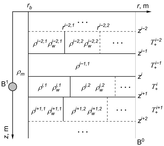
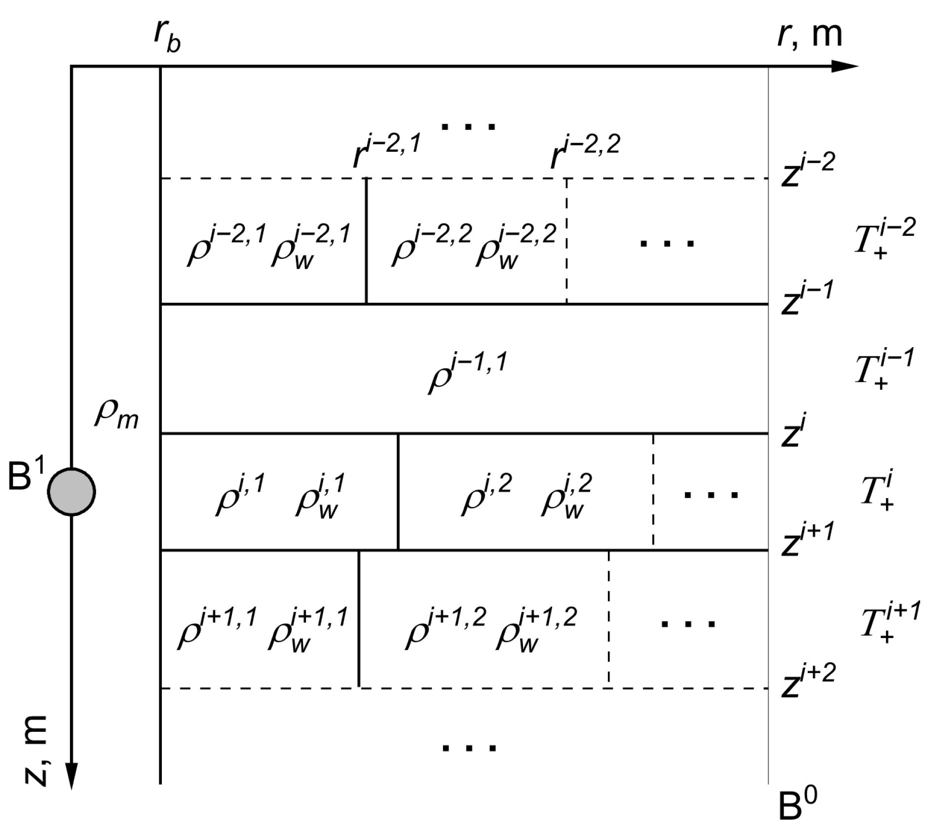
To solve the forward SP problem, we consider a model formulated in cylindrical coordinates (Figure 2). The vertical z-axis coincides with the borehole axis, and no dependence on the azimuthal angle is assumed (axisymmetric formulation). In the general case, the near-wellbore region within each permeable layer may consist of several coaxial cylindrical zones. Under these assumptions, Poisson’s Equation (3) can be written in the following form:
Figure 2.
Axisymmetric model of a medium including a borehole, multiple formations, and radial zones with different electrophysical properties.
As can be seen, the coefficient of the diffusion–adsorption electromotive force has a constant value in the radial direction and varies only along the z-axis, reflecting the lithological heterogeneity of the medium. At the same time, the electrical resistivity of the medium and the electrical resistivity of the pore fluid may differ both radially and vertically, depending on the spatial distribution of electrophysical parameters. Within the borehole, and are assumed to be equal and correspond to the electrical resistivity of the drilling mud .
To describe the potential distribution, it is also necessary to specify boundary conditions for the computational domain. The first boundary condition is applied at the surface of the measuring electrode . Since the electrode is not a current source, no current flows through its surface; this is expressed as a zero normal derivative of the potential:
The second boundary condition is specified at the outer boundary of the modeled domain , where the potential is assumed to be zero:
This condition corresponds to placing the boundary far from the region influenced by the current sources and ensures that the field decays at large distances from the borehole.
2.2.2. Implementation of the Finite Element Method
Equation (4), together with boundary conditions (5) and (6), defines a boundary-value problem for the potential in the axisymmetric domain shown in Figure 2. To solve this problem, a modified numerical algorithm based on the finite element method (FEM) is used. This approach has proven effective for lateral logging problems [22] and spontaneous potential logging [23]. The use of FEM is well suited in this problem because its variational formulation allows heterogeneous conductivity distributions and distributed source terms to be incorporated naturally, without introducing special approximations at the boundaries between zones.
For the numerical solution, the Poisson Equation (4) is considered in a two-dimensional domain with heterogeneous electrophysical properties.
The problem is formulated in a variational form, where the unknown potential and the test functions belong to the space , which vanishes at the outer boundary of the domain.
For the subsequent application of the finite element method, Equation (4) is rewritten in variational form. The objective is to find a potential function such that, for any test function , the following equality holds:
where describes the distribution of source currents.
This representation is equivalent to the original differential equation and satisfies the boundary conditions (5) and (6).
For an approximate solution of the variational problem, the potential is expanded in terms of a finite set of basis functions defined on the finite element mesh:
where are the expansion coefficients corresponding to the nodal values of the potential.
Substituting this expression into the variational equation and taking into account that any test function can be expanded on the same basis, we obtain a system of linear algebraic equations:
As a result of the discretization, the problem is reduced to solving this system of linear algebraic equations:
where the vector contains the coefficients of the potential expansion in terms of the basis functions.
The elements of the matrix and the right-hand side vector are determined by integration over the domain :
In the axisymmetric formulation, bilinear basis functions defined on a rectangular finite element mesh are used. The resulting matrix is symmetric and positive definite, which allows the system to be solved efficiently using the Cholesky method.
2.2.3. Parameterization of Electrophysical Properties and Current Sources
An important aspect of the numerical implementation is not only the choice of algorithm for solving the Poisson equation but also the proper parameterization of the distributions of the electrophysical properties and current sources specified in the right-hand side of the equation. In particular, both the radial and vertical components of the source current density must be taken into account. This allows the potential distribution near fluid contacts and at formation boundaries to be accurately described. The vertical variation in the potential strongly depends on the z-coordinate, which must be considered when modeling SP responses in media with thin or highly contrasting formations.
To define the right-hand-side function in Equation (4), it is necessary to specify the distributions of the formation resistivity , the fluid resistivity , and the cation transport number .
Since these parameters differ in the borehole and within each radial zone of the reservoirs, it is convenient to prescribe them as piecewise-constant functions in both coordinates r and z:
where is the electrical resistivity of the j-th radial zone of the i-th formation (layer), and is the Heaviside step function, defined as
is the radius of the j-th radial zone of the i-th formation, is the number of radial zones in formation i, and is the number of formations. An analogous expression can be written for and .
Since the Heaviside function is discontinuous, the stepwise parameter fields are approximated using smoothed transition functions and , which represent gradual changes in properties with radius and depth, respectively:
Sigmoid functions of the following form are employed as the transition functions:
where the parameters and determine the sharpness of the transitions in the radial and vertical directions, respectively. These parameters have the dimension of inverse length and define the characteristic width of the transition zones, which can be estimated as and . In the limit , the function reduces to the original stepwise model (12).
Approximating , and with smooth transition functions allows the derivatives in the right-hand side of the Poisson Equation (4) to be computed analytically:
To avoid excessive differentiation when the number of zones is large, the right-hand side is represented as the sum of local contributions from all radial and vertical boundaries:
For the vertical transition at the interface , the variation of can be described as
where defines the vicinity of the interface, and an analogous expression for .
The corresponding contribution to the right-hand side of the Poisson equation is then evaluated as
Analogously, for the radial transition at the interface :
with the following contribution to the right-hand side of the Poisson equation:
The decomposition is valid provided that the widths of the transition zones are much smaller than the distances between adjacent boundaries:
which prevents the overlap of adjacent transitions.
In this approximation, the right-hand side is constructed as a sum of independent smooth contributions, ensuring numerical stability and accuracy regardless of the number of radial and vertical zones. The use of multiple radial zones, in turn, enables flexible assignment of electrophysical parameters in the near-wellbore region. As the number of zones increases, the discrete parameterization converges toward a smooth radial profile that reflects the gradual invasion of the drilling mud filtrate into the formation and its mixing with the formation fluid. This representation provides a physically consistent description of the invasion zone and an accurate reproduction of the transitional processes between the borehole and the surrounding formation.
The expressions obtained for the right-hand-side function (16) are used to assemble the right-hand-side vector of system (10). The element integrals were evaluated using a numerical quadrature based on successive mesh refinement with Richardson extrapolation (Romberg-type integration) [24]. The integration procedure starts from a trapezoidal approximation and iteratively refines the discretization, while higher-order estimates of the integral are obtained through extrapolation of the results computed on consecutive refinement levels. The iterative process is terminated when the difference between successive approximations satisfies a prescribed tolerance. Despite the relative simplicity of this approach, the scheme provides numerical stability and independence from the predefined integration grid, which is especially important when the model geometry or the parameters of the radial zones are varied.
3. Results and Discussion
3.1. Validation of the Numerical Algorithm
Validation of the SP response modeling algorithm requires demonstrating its ability to accurately reproduce both the shape and the amplitude of the signal for a given set of geometric and electrophysical parameters. The response shape is primarily determined by the geometry of the beds and the distribution of electrical resistivity in the near-wellbore region, whereas the amplitude is controlled by electrochemical processes associated with ion diffusion. The electrochemical SP contribution is expressed in terms of formation-water resistivity , as this is standard in well-log interpretation and convenient for practical use. However, in the general case, a more accurate description is achieved in terms of electrolyte concentration (salinity), while the most rigorous thermodynamic approach is based on the use of ionic activities, as it accounts for deviations of real ion behavior in electrolyte solutions from the ideal case, which assumes the absence of interionic interactions, particularly at elevated salinities. In the implemented program, the conversion from to salinity is performed using an empirical relationship, whereas ionic activities are calculated using the Davies equation.
In previous studies [8,21], the electrochemical component of the SP response was also described using ionic activities, enabling a direct comparison of absolute SP response amplitudes with the results obtained in the present work. It should be noted, however, that the effect of electrical resistivity contrasts on the electrochemical component was not considered in those studies. Therefore, when reproducing the selected results, the electrical resistivity was assumed to be uniform throughout the entire modeling domain. All other modeling parameters were set in accordance with those used by the authors.
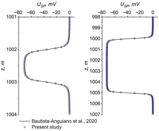
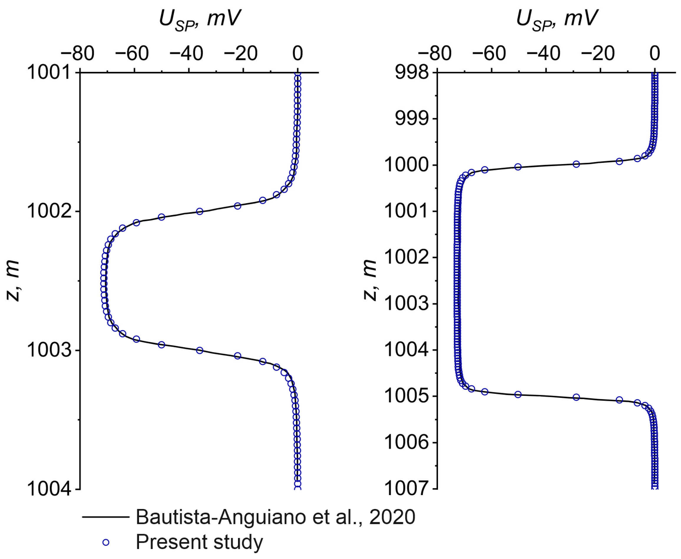
Figure 3 presents the results of SP response modeling for a three-layer medium, in which a permeable sandstone bed is bounded by two shale layers treated as ideal semipermeable membranes. The drilling mud salinity was set to 5 kppm, and the formation water salinity to 50 kppm. The borehole radius was set to 0.1 m. Comparison with the results reported in [8] demonstrates good agreement in both the shape and the amplitude of the SP curves, including the typical signal smoothing observed as the thickness of the permeable bed decreases. Furthermore, in the same study, the numerical modeling results were also compared with those reported in [9], allowing the present analysis to serve as a validation of the implemented algorithm against both approaches.
Figure 3.
Comparison of the calculated SP responses for a three-layer medium with the results reported in [8]. (Left): permeable bed thickness of 1 m; (right): permeable bed thickness of 5 m.
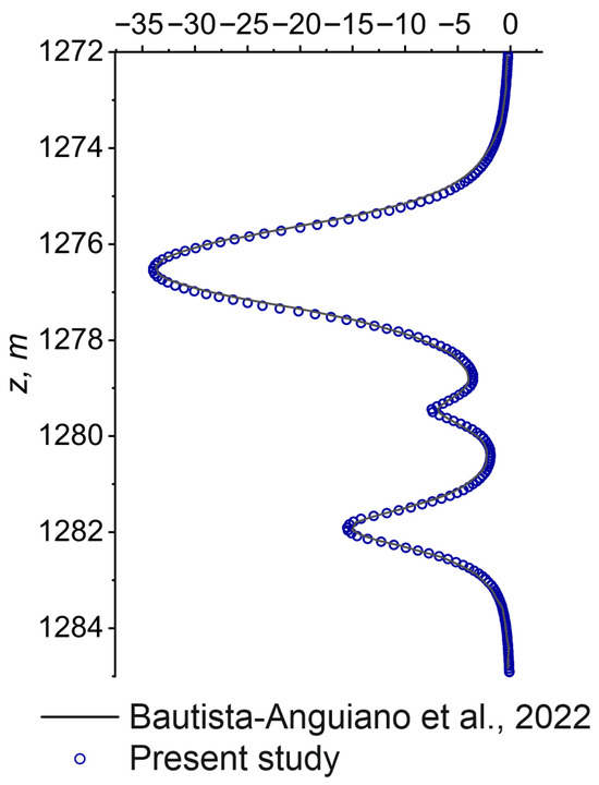
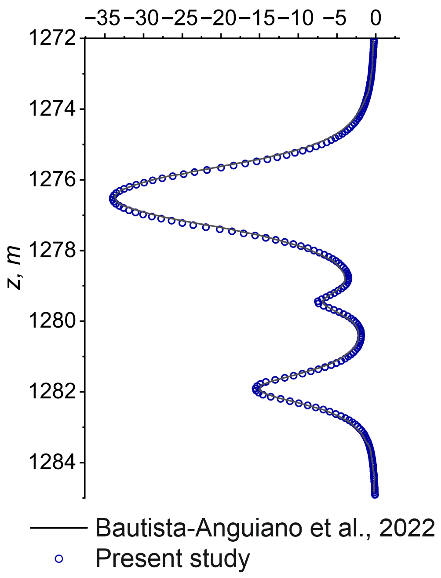
Correct treatment of the mud-filtrate invasion zone also plays a key role in validating the computational algorithm. As noted above, increasing the invasion radius leads to a reduction in the SP response amplitude, with this effect being most pronounced for thin beds. Figure 4 shows the modeling results for the medium considered in [21], which includes three permeable beds of varying thicknesses and different depths of mud-filtrate invasion (0.843 m, 0.473 m, and 0.646 m, respectively), bounded by impermeable shale layers. As in the previous example, electrical resistivity was assumed to be uniform throughout the modeling domain to allow a consistent comparison. The drilling mud salinity was set to 7.5 kppm and the formation water salinity to 60 kppm. The borehole radius was set to 0.1 m. The results are in good agreement with the data reported in [21], confirming that the invasion zone is correctly treated in the absence of resistivity-contrast effects.
Figure 4.
Comparison of the calculated SP responses for a medium with a mud-filtrate invasion zone with the results reported in [21].
The numerical modeling results obtained allow a clear analysis of the influence of bed thickness and invasion-zone width on the shape and amplitude of the SP responses, as well as an assessment of the correct implementation of the electrochemical SP source. However, as is well known, heterogeneity in the resistivity distribution of the medium also affects the SP response [1,3]. Accounting for this factor requires a more complex medium model and additional validation of the algorithm.
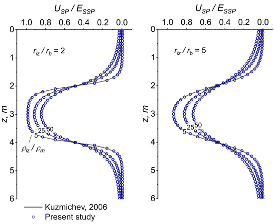
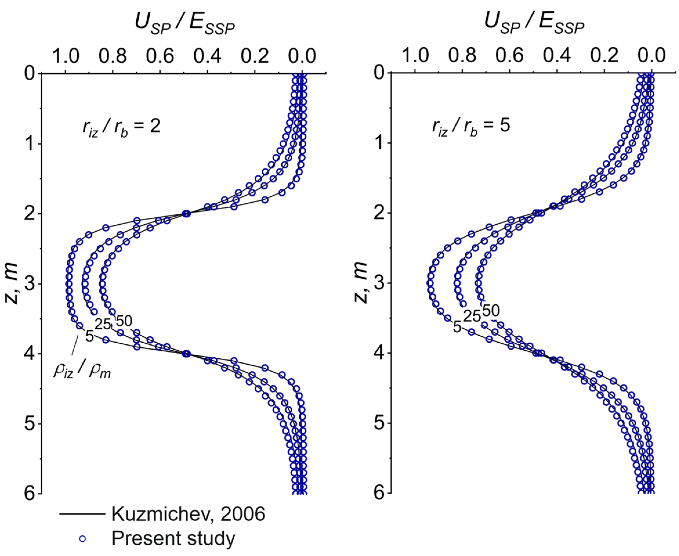
In a previous study [23], the effect of resistivity contrast between the borehole and the surrounding formations was demonstrated, while a more general case is considered here. Figure 5 presents a comparison between the numerical modeling results and the analytical solution from [25]. Although this solution does not consider the resistivity of the shale shoulder beds, it allows one to evaluate the effect of resistivity contrast between the borehole, the invasion zone, and the uninvaded part of the permeable bed for an arbitrary invasion zone width.
Figure 5.
Comparison of the calculated SP responses with the analytical solution from [25] for different resistivity ratios (indicated in the curve labels) between the invasion zone and the borehole. (Left): invasion zone radius equal to twice the borehole radius; (right): invasion zone radius equal to five times the borehole radius. The resistivity of the invasion zone is five times that of the uninvaded part of the permeable bed.
For a more comprehensive description of SP responses that includes the effect of the resistivity of the adjacent formations, no analytical solution is available. One of the tools that allows the combined effects of resistivity distribution to be taken into account is the use of correction charts, which show the dependence of normalized SP amplitude on the thickness of the permeable bed for different resistivity ratios between the borehole, the invasion zone, the surrounding shale layers, and the uninvaded part of the reservoir.
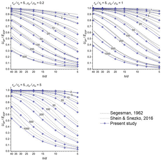
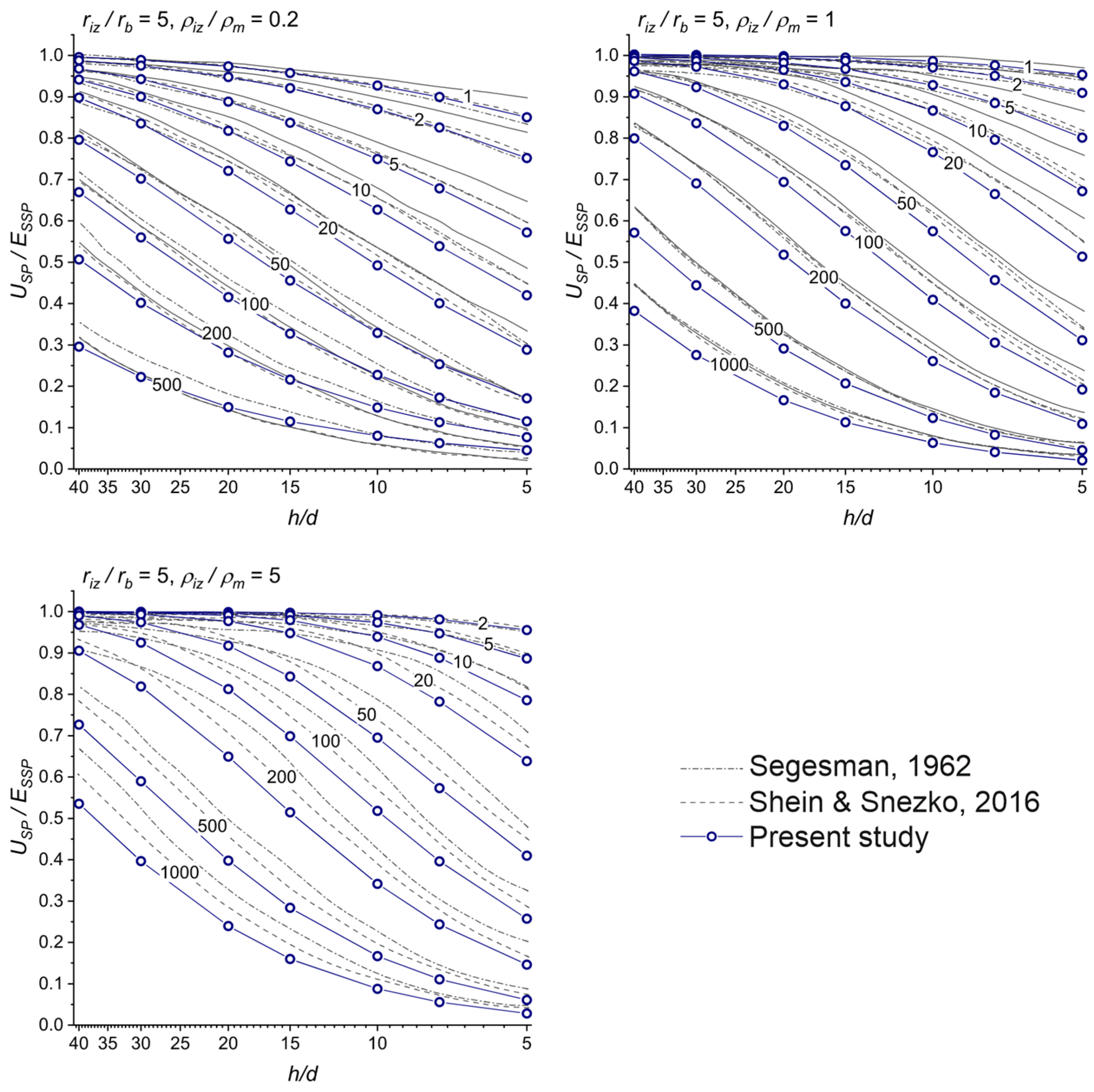
The original correction charts were obtained in [3] using an equivalent resistive network and are still included in the official Schlumberger chart book [26]. Similar relationships were later reproduced using numerical modeling in [27]. Figure 6 presents a comparison of our numerical modeling results with the digitized charts from [3,27] for a resistivity ratio of 20 between the borehole and the adjacent formations.
Figure 6.
Comparison of calculated normalized SP responses with the correction charts from [3,27]. Each subplot corresponds to a different resistivity ratio between the invasion zone and the borehole. Curve labels indicate the resistivity ratio between the invasion zone and the uninvaded part of the permeable formation. The resistivity of the adjacent formations is 20 times that of the borehole.
All charts exhibit similar qualitative behavior; however, quantitative differences of up to approximately 10% are observed both among previously published charts and between those charts and our calculations. Our numerical modeling results show a more pronounced reduction in SP amplitude, particularly when the resistivity of the invasion zone is higher than that of the uninvaded part of the permeable bed. Definitive validation would require experimental data and systematic analysis, which are not currently available in the open literature.
Nevertheless, each of the provided validation examples has inherent limitations that should be acknowledged. Analytical solutions, such as that used in Figure 5, are available only for simplified geometries and resistivity distributions and therefore cannot serve as a comprehensive benchmark for the full range of model complexity considered here. Previously published numerical results [8,21] provide a more direct basis for comparison but are themselves subject to modeling assumptions that partially overlap with our own, limiting their independence as validation references. Correction charts [3,26,27], while widely used in practice, were derived from equivalent resistive network models and are known to be approximate; the quantitative discrepancies of up to 10% observed in Figure 6 likely reflect differences in underlying modeling assumptions rather than errors in any single implementation. Most importantly, no experimental benchmark, such as laboratory measurements on physical models or well-controlled field data with independently verified ground truth, is currently available in the open literature for this class of problems. This absence is a recognized limitation of the field as a whole and is not specific to the present study. Taken together, the available validation evidence supports the correctness of the implemented algorithm within the tested parameter range, but a definitive quantitative assessment of its accuracy under the full range of field conditions remains an open problem that will ultimately require dedicated experimental datasets to be properly resolved.
3.2. Practical Example (Southeast Asia Natural Gas Field)
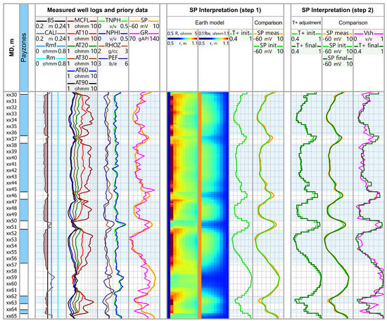
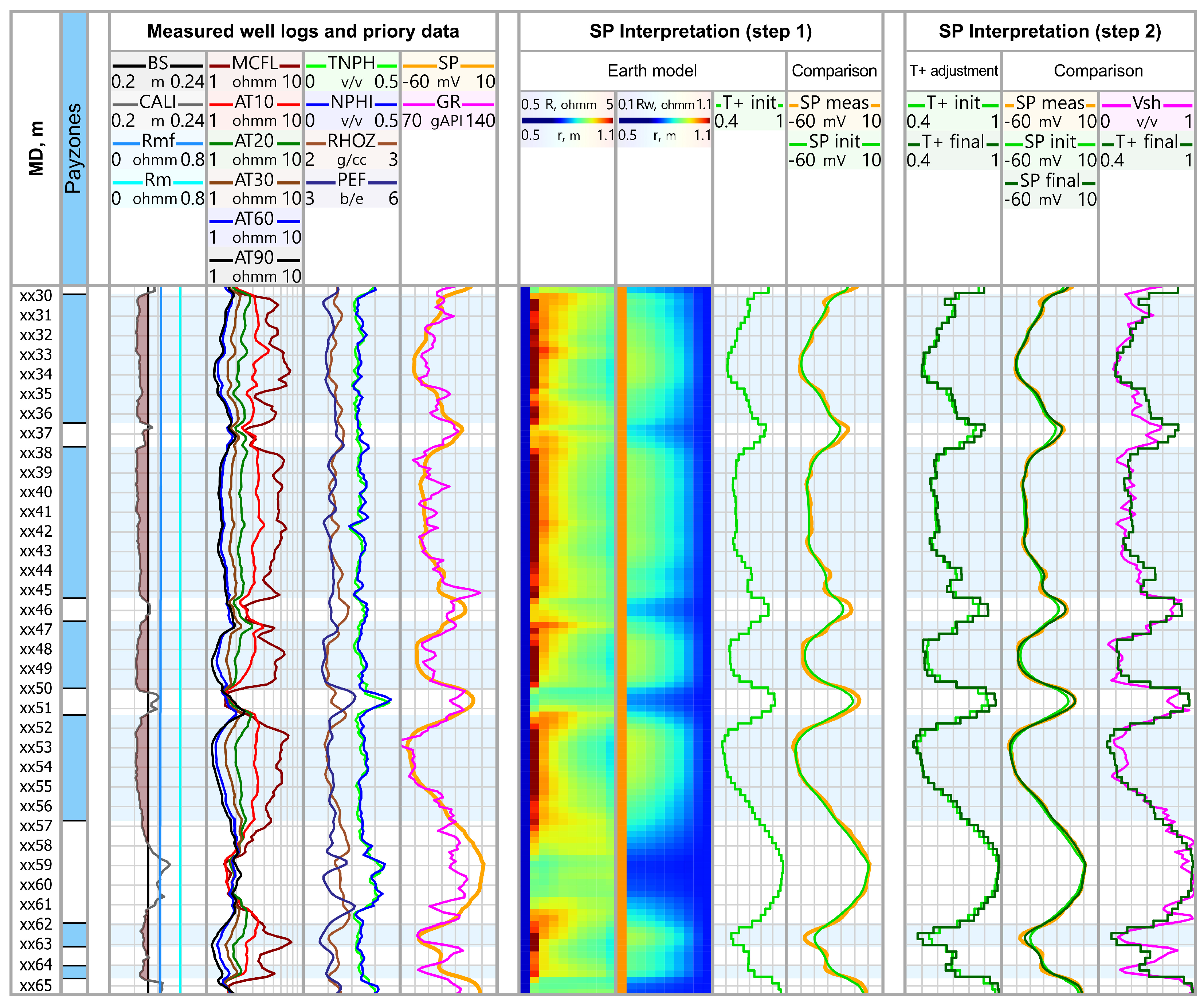
The developed algorithm can be applied to the interpretation of field SP data. As an example, we consider modeling results for an interval of interbedded water-saturated sand-shale deposits of Upper Miocene age (inner-shelf marine sediments) from a Southeast Asian natural gas field (Figure 7). The predominantly water-saturated nature of the formation allows SP data to be interpreted with an evaluation of formation water salinity and the cation transport number () while requiring minimal a priori information. Correlation of SP data with gamma-ray (GR) log and salinity estimates obtained from resistivity logs suggests that the water salinity remains largely constant over the interval and that variations in the SP response can be attributed primarily to changes in .
Figure 7.
Application of the developed algorithm to the interpretation of field SP data. From (left) to (right): reservoir flag; measured well log data; initial earth model and comparison of simulated SP logs with the measured data (step 1); final interpretation results (step 2) and comparison of the derived cation transport number with .
As input data for SP modeling, the following information was used: borehole caliper measurements; a smooth resistivity model derived from array induction tool (AIT) and micro-cylindrically focused logging (MCFL) data; the electrical resistivity of the drilling mud; and the resistivity of the mud filtrate, calculated based on the drilling mud properties using the Overton & Lipson model [26].
The interpretation was carried out in two steps. In the first step, formation water salinity was estimated (assumed uniform across the interval). Initial values of the cation transport number were assigned based on the SP response: for the cleanest sandstones, was set to 0.4, and for the most shale-rich intervals was set to 1.0. For sandstone intervals with intermediate shale content, was assumed proportional to the observed SP response. As a result, a formation water salinity of 37 kppm was determined, which agrees well with estimates from the established petrophysical model for the deposits (36–39 kppm). The synthetic SP curve calculated using these parameters is labeled as “SP init” in the figure. As seen, there is good agreement between the synthetic and measured data for the thickest reservoir intervals, whereas for thinner beds, discrepancies are observed, which can be attributed to the neglect of the effect of surrounding formations in the initial estimation. It should be noted that the initial assignment of values is based on heuristic assumptions reflecting the expected range between clean sandstones and shale-rich intervals and that the assumption of uniform formation water salinity represents a prior constraint that influences the inversion results. This assumption is, however, physically motivated and supported by independent resistivity-based salinity estimates showing no systematic depth trend over the studied interval, as well as by consistency with the established regional petrophysical model for these deposits. Similarly, the restriction of to depth-only variations is a simplifying assumption adopted for this particular example rather than a fundamental limitation of the proposed algorithm, which supports radially varying without any modification to the underlying formulation; introducing radial heterogeneity of would, however, substantially increase the non-uniqueness of the interpretation problem and would require additional independent constraints, such as radially resolved clay content estimates, that are not available for the current dataset.
Therefore, in the second step, the previously determined formation water salinity was held constant, while the initial values were refined to minimize the misfit between measured and synthetic SP data. The final outcome of the interpretation includes the estimated formation water salinity and the profile as a function of depth. The comparison shown on the rightmost track between the derived values and the curve obtained from GR, Neutron, and Density logs shows good correlation, confirming both the validity of the interpretation assumption of uniform formation water salinity and the overall correctness of the implemented algorithm.
4. Discussion
Above, we intentionally considered only the water-bearing interval with uniform formation water salinity. This allowed us to separate the demonstration of the correctness of the developed algorithm from issues related to the petrophysical interpretation of well log data. In practice, the primary interest lies in hydrocarbon-bearing intervals. It is also important to note that the cation transport number is a physico-chemical parameter that itself requires petrophysical interpretation. Such an interpretation can, for example, be performed using the Waxman–Smits model [13,28], within which is expressed as follows:
where is the porosity, is the water saturation, is the effective mobility of cations on the mineral surface, is the solid phase density (2650 kg·m−3 for silica), is the cation exchange capacity and is the microscopic Hittorff number (0.4 for NaCl solution), determined by the relative mobility of cations in the free electrolyte.
It is important to emphasize that the decomposition of the SP response into contributions from formation water salinity and the cation transport number is physically motivated but not mathematically unique in the general case. Different combinations of these parameters may produce similar SP responses, which reflects the inherent non-uniqueness of the inversion problem. In this study, additional constraints are introduced through geological context and independent petrophysical information; however, a formal uncertainty analysis is beyond the scope of the present work and remains a subject for future investigation.
The dependence of on formation water salinity, porosity, saturation, and cation exchange capacity requires additional information to estimate these parameters in intervals with mixed saturation, depth-varying clay mineralogy, and/or variable water salinity. Under such conditions, it is more appropriate to treat SP modeling not as a method for direct estimation of a specific petrophysical parameter, but rather as a tool that provides an additional independent equation within a comprehensive petrophysical interpretation. This approach enables the evaluation of various parameters depending on the available data and the geological characteristics of the section.
Another aspect worth noting is computational efficiency. The present study considers a 2D formulation, which offers a reasonable compromise for the analysis of data acquired in vertical and low-to-moderate inclination wells. Even so, the computation is not trivial: assembly of the right-hand-side vector in system (10) requires numerical integration of the source term over the entire mesh, and for fine discretizations or models with many radial zones, this step dominates the runtime. In the current implementation, a single forward simulation for a logging interval comparable to that shown in Figure 7 (35 m, 120 layers, 10 radial zones per layer, ~106 finite elements combined) requires approximately 15 min on a single thread of an AMD Ryzen 9 7950X workstation. While acceptable for research-oriented forward modeling, this runtime makes iterative inversion impractical under field conditions. Extension to a full 3D formulation introduces no fundamental mathematical differences, but the computational cost scales prohibitively, making direct 3D inversion infeasible with current hardware.
In addition to the obvious solution of parallelizing the computations, another promising approach is the construction of a deep-learning-based accelerated model of the numerical solver. Such solutions have already been explored in well logging for other methods, both for forward [29,30] and inverse simulations [31,32]. The present problem, however, poses additional challenges: the SP response depends simultaneously on spatial distributions of formation resistivity, pore-fluid resistivity, and the cation transport number in both the radial and vertical directions, resulting in a high-dimensional input space that requires a more expressive network architecture and a carefully designed training dataset. Addressing these challenges, including the generation of a sufficiently diverse synthetic training set and validation against the FEM solver across a representative range of geological scenarios, will be the focus of future work.
5. Conclusions
In this study, we present a novel finite element-based algorithm for modeling SP well logs in complex near-wellbore environments. The proposed approach combines a physically consistent description of electrochemical SP generation mechanisms with a flexible parameterization of electrophysical properties. Unlike conventional methods that use simplified analytical models and correction charts, the proposed formulation explicitly accounts for shale content via the cation transport number and models smooth radial variations in formation and pore-fluid resistivity near the wellbore.
The numerical implementation was validated against previously published analytical and numerical solutions, demonstrating good agreement in terms of both SP response amplitude and shape under a range of model conditions. The results confirm that the algorithm adequately captures the influence of key factors, including bed thickness, invasion-zone geometry, and resistivity contrasts. At the same time, some discrepancies with existing correction charts highlight the sensitivity of the SP response to modeling assumptions and emphasize the need for further verification, particularly in the absence of comprehensive experimental benchmarks.
Application of the method to field data illustrates its practical potential for interpreting SP logs in shaly sand reservoirs. In the considered example, the approach provides reliable estimates of formation water salinity and the cation transport number. These results suggest that the method can be used as an additional tool within integrated petrophysical interpretation workflows, especially in cases where available data are limited.
It should be noted, however, that the proposed approach does not eliminate the inherent non-uniqueness of SP log interpretation and still requires auxiliary information for reliable estimation of formation parameters in more complex geological settings. Furthermore, computational efficiency remains an important consideration, particularly for potential extensions to three-dimensional problems. Future work will focus on accelerating the forward solver through deep learning to enable practical inversion in large logging intervals and extension to more complex reservoir conditions with mixed hydrocarbon–water saturation.
Author Contributions
Conceptualization, K.D.; methodology, K.D. and A.G.; software, K.D. and A.G.; validation, A.G. and A.P.; writing—original draft preparation, K.D., A.G. and A.P.; visualization, A.G. and A.P.; project administration, K.D.; funding acquisition, K.D. All authors have read and agreed to the published version of the manuscript.
Funding
This research was funded by the Russian Science Foundation, grant number 25-77-00054 “Advanced software-algorithmic solutions for the interpretation of spontaneous potential logging data in hydrodynamically consistent models of shaly fluid-saturated sediments through numerical simulation and deep learning”.
Data Availability Statement
The data generated and analyzed during the current study are available from the corresponding author on reasonable request.
Conflicts of Interest
The authors declare no conflicts of interest.
Abbreviations
The following abbreviations are used in this manuscript:
| AIT | Array Induction Tool |
| CEC | Cation Exchange Capacity |
| EMF | Electromotive Force |
| FEM | Finite Element Method |
| GR | Gamma Ray |
| MCFL | Micro-Cylindrically Focused Logging |
| SP | Spontaneous Potential |
| Cation Transport Number | |
| Shale Volume Fraction |
References
- Doll, H.G. The S.P. Log: Theoretical Analysis and Principles of Interpretation. Trans. AIME 1949, 179, 146–185. [Google Scholar] [CrossRef] [Scilit]
- Worthington, A.E.; Meldau, R.F. Departure Curves for the Self-Potential Log. Trans. AIME 1958, 213, 11–16. [Google Scholar] [CrossRef] [Scilit]
- Segesman, F. New SP Correction Charts. Geophysics 1962, 27, 815–828. [Google Scholar] [CrossRef] [Scilit]
- Revil, A. Ionic Diffusivity, Electrical Conductivity, Membrane and Thermoelectric Potentials in Colloids and Granular Porous Media: A Unified Model. J. Colloid Interface Sci. 1999, 212, 503–522. [Google Scholar] [CrossRef] [Scilit]
- Li, T.; Tan, Y.; Peng, Y. Mathematical Model and Method for Spontaneous Potential Well Logging. Eur. J. Appl. Math. 1994, 5, 123–139. [Google Scholar] [CrossRef] [Scilit]
- Zhang, G.J.; Wang, G.L. Application of vector potential theory to spontaneous potential computation. Radio Sci. 1997, 32, 899–905. [Google Scholar] [CrossRef] [Scilit]
- Pan, K.J.; Tan, Y.J.; Hu, H.L. Mathematical Model and Numerical Method for Spontaneous Potential Log in Heterogeneous Formations. Appl. Math. Mech. 2009, 30, 209–219. [Google Scholar] [CrossRef] [Scilit]
- Bautista-Anguiano, J.; Torres-Verdín, C.; Strobel, J. Mechanistic 3D Finite-Difference Simulation of Borehole Spontaneous Potential Measurements. Geophysics 2020, 85, D105–D119. [Google Scholar] [CrossRef] [Scilit]
- Zhang, G.J.; Wang, G.L. A New Approach to SP Computation-Vector Potential Approach. IEEE Trans. Geosci. Remote Sens. 1999, 37, 2092–2098. [Google Scholar] [CrossRef] [Scilit]
- Zhao, P.; Wang, Y.; Li, G.; Hu, C.; Xie, J.; Duan, W.; Mao, Z. Joint Inversion of Saturation and Qv in Low-Permeability Sandstones Using Spontaneous Potential and Resistivity Logs. Petrophysics 2023, 64, 741–752. [Google Scholar] [CrossRef] [Scilit]
- Sill, W.R. Self-Potential Modeling from Primary Flows. Geophysics 1983, 48, 76–86. [Google Scholar] [CrossRef] [Scilit]
- Revil, A.; Jougnot, D. Diffusion of ions in unsaturated porous materials. J. Colloid Interface Sci. 2008, 319, 226–235. [Google Scholar] [CrossRef] [Scilit]
- Woodruff, W.F.; Revil, A.; Jardani, A.; Nummedal, D.; Cumella, S. Stochastic Bayesian Inversion of Borehole Self-Potential Measurements. Geophys. J. Int. 2010, 183, 748–764. [Google Scholar] [CrossRef] [Scilit]
- Salazar, J.M.; Wang, G.L.; Torres-Verdín, C.; Lee, H.J. Combined simulation and inversion of SP and resistivity logs for the estimation of connate-water resistivity and Archie’s cementation exponent. Geophysics 2008, 73, E107–E114. [Google Scholar] [CrossRef] [Scilit]
- Kuzmichev, O.B.; Zhonin, A.V.; Martynova, Y.V.; Kolomasova, S.A. Solution of the Inverse Problem of Self-Polarization Logging in a Pack of Layers with a Penetration Zone (Terrigenous Section). Oil Ind. 2019, 10, 38–41. [Google Scholar] [CrossRef] [Scilit]
- Dakhnov, V.N. Prospective Geophysics; Pershina, V.G., Fedotova, I.G., Eds.; State Scientific and Technical Publishing House of Oil and Mining and Fuel Literature: Moscow, Russia, 1959. (In Russian) [Google Scholar]
- Pirson, S.J. Oil Reservoir Engineering, 2nd ed.; McGraw-Hill: New York, NY, USA, 1958. [Google Scholar]
- Jiao, D.; Sharma, M. An Experimental Investigation of the Resistivity Profile in the Flushed Zone. Log. Anal. 1992, 33, 145–154. [Google Scholar]
- Allen, D.; Auzerias, F.; Dussan, E.; Goode, P.; Ramakrishnan, T.S.; Schwartz, L.; Wilkinson, D.; Fordham, E.; Hammond, P.; Williams, R. Invasion Revisited. Oilfield Rev. 1991, 3, 10–23. [Google Scholar]
- Revil, A.; Linde, N. Chemico-Electromechanical Coupling in Microporous Media. J. Colloid Interface Sci. 2006, 302, 682–694. [Google Scholar] [CrossRef] [Scilit]
- Bautista-Anguiano, J.; Torres-Verdín, C. Inversion-Based Interpretation of Borehole Spontaneous Potential Measurements for Accurate Estimation of Water Resistivity in the Presence of Shoulder-Bed and Mud-Filtrate Invasion Effects. Geophysics 2022, 87, D47–D65. [Google Scholar] [CrossRef] [Scilit]
- Nechaev, O.V.; Glinskikh, V.N. Three-dimensional simulation and inversion of lateral logging sounding and lateral logging data in media with tilt of the main axes of the dielectric anisotropy tensor. Vestn. NSU 2018, 16, 127–139. [Google Scholar] [CrossRef] [Scilit]
- Epov, M.; Glinskikh, A.; Nechaev, O. Finite-Element Modeling of Spontaneous Potential in an Axisymmetric Reservoir Model with Account of Its Shale Content. Geosciences 2022, 12, 30. [Google Scholar] [CrossRef] [Scilit]
- Romberg, W. Vereinfachte numerische Integration. Det. K. Nor. Vidensk. Selsk. Forh. 1955, 28, 30–36. (In German) [Google Scholar]
- Kuzmichev, O.B. Investigation of Natural Electric Fields in Oil and Gas Exploration Wells (Theory, Instrumentation, Methodology, Borehole Tests); Nedra LLC: St. Petersburg, Russia, 2006; 252p. (In Russian) [Google Scholar]
- Schlumberger. Log Interpretation Charts; Schlumberger: Houston, TX, USA, 2013. [Google Scholar]
- Shein, Y.L.; Snezhko, O.M. A Solution of the Direct and Inverse Problems in The Spontaneous Potential Technique for the Formation Bundle. A Practical Application. Karotazhnik 2016, 9, 156–171. (In Russian) [Google Scholar]
- Waxman, M.H.; Smits, L.J.M. Electrical Conductivities in Oil-Bearing Shaly Sands. Soc. Pet. Eng. J. 1968, 8, 107–122. [Google Scholar] [CrossRef] [Scilit]
- Hagiwara, T. Machine-Learning-Based Convolution Method for Fast Forward Modeling of Induction Log. Petrophysics 2023, 64, 312–322. [Google Scholar] [CrossRef] [Scilit]
- Petrov, A.M.; Leonenko, A.R.; Danilovskiy, K.N.; Nechaev, O.V. Fast 2D Forward Modeling of Electromagnetic Propagation Well Logs Using Finite Element Method and Data-Driven Deep Learning. Artif. Intell. Geosci. 2025, 6, 100112. [Google Scholar] [CrossRef] [Scilit]
- Hagiwara, T. Machine-Learning-Based Deconvolution Method Provides High-Resolution Fast Inversion of Induction Log Data. Petrophysics 2023, 64, 304–311. [Google Scholar] [CrossRef] [Scilit]
- Leonenko, A.R.; Petrov, A.M.; Danilovskiy, K.N. A method for correction of shoulder-bed effect on resistivity logs based on a convolutional neural network. Russ. Geol. Geophys. 2023, 64, 1058–1064. [Google Scholar] [CrossRef] [Scilit]
Disclaimer/Publisher’s Note: The statements, opinions and data contained in all publications are solely those of the individual author(s) and contributor(s) and not of MDPI and/or the editor(s). MDPI and/or the editor(s) disclaim responsibility for any injury to people or property resulting from any ideas, methods, instructions or products referred to in the content. |
© 2026 by the authors. Licensee MDPI, Basel, Switzerland. This article is an open access article distributed under the terms and conditions of the Creative Commons Attribution (CC BY) license.