Rainfall-Induced Landslide Stability for Variably Shaped Slopes: A Multi-Model Integration Approach Through Green-Ampt Theory and Numerical Validation

Abstract

As one of the most catastrophic geological hazards globally, landslides exhibit heightened risks due to their increasing frequency, destructive potential, and extensive spatial distribution. The primary objective of this study is to develop an integrated analytical framework to quantitatively evaluate the stability of variably shaped slopes under rainfall infiltration. The core hypothesis is that slope curvature significantly alters infiltration behavior and stress distribution, leading to morphology-dependent failure mechanisms. Employing Green-Ampt infiltration theory coupled with limit equilibrium analysis, we establish stability prediction models for three fundamental slope geometries (linear, concave, convex) under contrasting rainfall regimes (high-intensity vs. low-intensity precipitation). The derived analytical solutions reveal two critical phenomena: (1) progressive downward migration of the saturation front maintaining parallelism with slope surfaces during infiltration and (2) time-dependent stability deterioration following hyperbolic decay patterns. The proposed models are rigorously validated through numerical simulations employing finite element methods, which demonstrate remarkable congruence with theoretical predictions, showing safety factor discrepancies below 5% (ΔFs < 0.05). Particularly, concave slopes exhibit 18–22% faster destabilization rates compared to convex counterparts under equivalent rainfall conditions. The validated models elucidate the spatiotemporal evolution of matric suction and pore pressure distributions, providing quantitative insights into morphology-dependent failure thresholds. These findings advance predictive capabilities for rainfall-induced landslides through physics-based stability criteria, offering critical guidance for terrain-specific early warning systems and mitigation strategies in geohazard-prone regions.

1. Introduction

Landslides are typical geological disasters characterized by complex formation mechanisms and strong destructive power. They are recognized as one of the most critical and hazardous geological hazards worldwide [1,2,3]. China has complex geological conditions, diverse landforms, and variable climatic environments. As a result, China experiences one of the highest frequencies of landslide disasters globally. These disasters have caused severe losses to the safety of people’s lives and property [4,5,6] Accordingly, strengthening landslide research is of great significance for geological disaster prevention and reduction [7,8].

Rainfall is one of the most common triggering factors of landslide [9]. Specifically, the impact of rainfall on slope is mainly reflected in the following three aspects: (1) rainfall will increase the water content of the slope, which tends to increase the sliding force of slope [9,10,11]; (2) the matrix suction in the slope and the mechanical properties of soil will be weakened by the rainfall infiltration, reducing the anti-sliding force of the slope [12]; (3) the groundwater level is prone to rise from rainfall infiltration, which has a detrimental impact on the stress state and slope structure [13,14]. Therefore, it is necessary to study the infiltration law of slope under the action of rainfall for slope stability analysis and prevention [15]. Regarding the theoretical research, many rainfall infiltration models have been proposed and improved gradually, such as Green-Ampt model (GA model) [16], Richards model [17], Mein–Larson model (ML model) [18], etc. Whereafter, GA model has been improved by many scholars [19,20,21,22]. In recent years, the application of GA model has been further developed under complex conditions, such as layered soil [23,24,25], fissured soil [26], unsaturated flows [27], semi-arid basins [28], hemispherical infiltration [29], and 3D slope stability. These models mostly focus on parameter improvement and application under complex conditions, while there are few studies on rainfall infiltration models with different slope forms.

Slopes in nature are usually not linear, but a curved shape or stepped shape. Qiao et al. (2006) divided the landslides of the Three Gorges reservoir area into five shapes, of which the curved slope accounted for about 88% [30]. However, the shape of the slope exerts a considerable influence on its stress state and hydrological response [31,32]. Recent studies have demonstrated that different slope curvatures produce distinct stress distributions, leading to varying stability behaviors under identical rainfall conditions [33,34]. Sannino et al. [35] provided a comprehensive review of physically based distributed models for rainfall-induced shallow landslides, emphasizing that topographic curvature is a critical factor controlling failure initiation and should be explicitly incorporated into stability assessments. Moradi et al. [36] compared different coupling strategies in hydromechanical models and revealed that slope geometry significantly affects the infiltration–stability relationship, with convex slopes exhibiting faster pore pressure responses and earlier failure compared to concave slopes under the same rainfall intensity. Zhou et al. [37] investigated the response patterns of soil water recharge on slopes with different curvatures and established quantitative relationships between slope shape and rainfall infiltration efficiency, demonstrating that concave slopes retain moisture longer while convex slopes drain more rapidly. Tang et al. [31] developed numerical models for multi-layered slopes that explicitly account for slope geometry effects on hydrological mechanisms and failure timing, confirming that curvature-dependent stress redistribution plays a key role in slope instability processes. Recent advances in landslide hydrology have progressed along three complementary directions: (1) rainfall threshold studies establishing empirical intensity–duration relationships for early warning [38,39]; (2) hydrological slope stability modeling coupling distributed hydrological models with stability analysis [40,41]; and (3) coupled hydromechanical approaches incorporating unsaturated soil behavior and pore pressure–mechanical interactions [42,43]. While these approaches have significantly advanced the field, a gap remains in the analytical treatment of slope curvature effects on rainfall infiltration and stability—most existing analytical frameworks assume linear slope geometry or treat curvature empirically. This study aims to fill this gap by extending the classical Green-Ampt infiltration model to concave and convex slopes through the introduction of a position-dependent equivalent slope angle.

Despite the widespread application of Green-Ampt-based models in slope stability analysis, existing studies predominantly focus on linear slopes with simplified geometry, leaving the analytical treatment of slope curvature—particularly its explicit integration into both infiltration and stability calculations—largely unexplored. This study addresses this gap by developing a unified analytical framework that quantitatively links slope morphology (concave, convex, linear) to rainfall-induced failure mechanisms. The main novelty lies in (1) the theoretical extension of the classical Green-Ampt model to variably shaped slopes via a position-dependent equivalent slope angle, enabling quantitative analytical characterization of curvature–infiltration links; (2) the derivation of closed-form stability solutions that explicitly incorporate slope curvature as a controlling parameter, quantifying geometry–failure timing relationships; and (3) systematic validation against independent numerical simulations, with statistical error metrics (RMSE = 0.018, R² = 0.976) confirming the framework’s accuracy and reliability. Unlike existing infiltration–stability coupled models, our approach uniquely integrates unified multi-morphology treatment, rigorous curvature-incorporating analytical derivation, and comprehensive numerical verification. The model provides new insights into morphology-dependent failure behavior—for instance, concave slopes destabilize 18–22% faster than convex slopes under identical rainfall—offering a physics-based foundation for terrain-specific early warning and hazard assessment.

2. Rainfall Infiltration Models

2.1. Geological Models of Different Slope Shapes

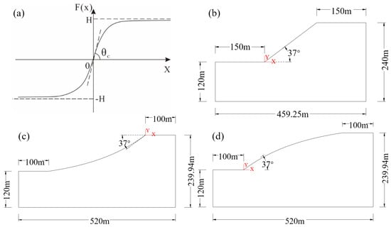
Slope morphology can be portrayed by function curve. Currently, slope morphology is described by exponential, logarithmic, and hyperbolic functions. For the sake of convenience, this paper assumed that slope geometry satisfies an exponential function and established a global coordinate system with slope midpoint as the origin, then slope function can be expressed as

$$F(x)=\left\{\begin{array}{cc}-H\left[1-\exp \left({\displaystyle \frac{x}{H}}\tan {\theta }_c\right)\right]\hfill & x<0\hfill \\ H\left[1-\exp \left(-{\displaystyle \frac{x}{H}}\tan {\theta }_c\right)\right]\hfill & x\ge 0\hfill \end{array}\right.$$

(1)

where θ_c is denoted as the maximum equivalent slope angle and H as the equivalent height of slope. Slope surface curve is shown in Figure 1a.

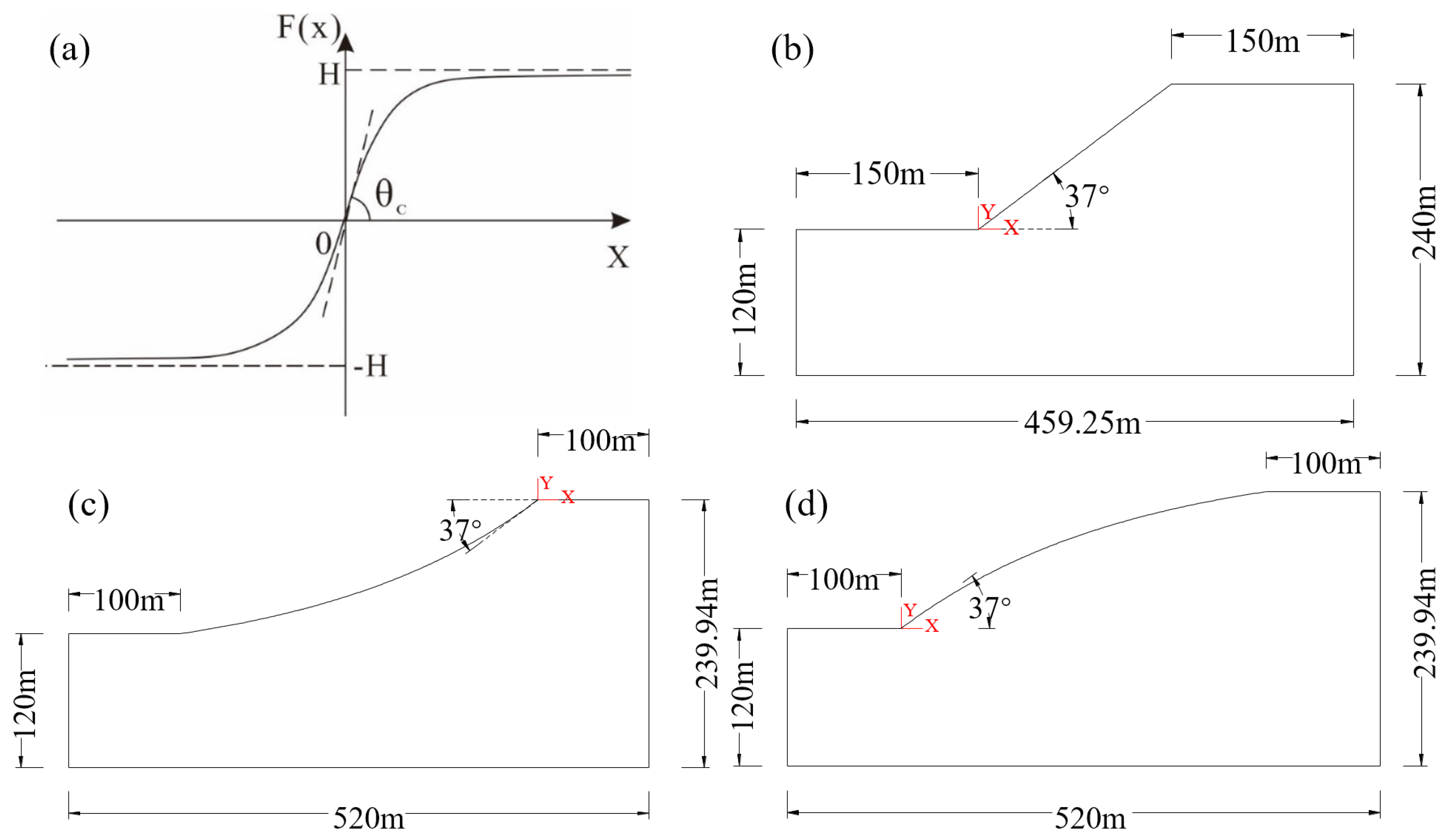
Figure 1. (a) Slope function curve, (b) Geological model of linear slope, (c) Geological model of concave slope, (d) Geological model of convex slope.

As demonstrated by Figure 1, the degree of concave and convex can be converted by changing the values of θ_c and H. For concave slopes, the slope function curve in the interval (x < 0) can be selected to describe the shapes, in which the top of the slope is located at the origin and there is a maximum equivalent slope angle θ_c. That is, the slope function of the concave slope is

$$F(x)=H\left[1-\exp \left({\displaystyle \frac{x}{H}}\tan {\theta }_c\right)\right],x<0$$

(2)

For any point P(x,y) on the concave slope surface, the tangent slope f(x) of this point can be obtained as Equation (3):

$$f(x)=\tan {\theta }_c\cdot \exp \left({\displaystyle \frac{x}{H}}\tan {\theta }_c\right),x<0$$

(3)

For convex slopes, to facilitate the study of the stability calculation model, the convex slope function curve can be described by moving the slope function in the interval (x > 0) down by h and moving to the left by ω, the top of the slope is located at the origin, and there is a maximum equivalent slope angle θ_c at the toe. That is, the slope function of the convex slope is

$$F(x)=H\left[1-\exp \left(-{\displaystyle \frac{x+\omega }{H}}\tan {\theta }_c\right)\right]-h,x<0$$

(4)

For any point P(x,y) on the convex slope surface, the tangent slope f(x) of this point can be obtained as Equation (5):

$$f(x)=\tan {\theta }_c\cdot \exp \left(-{\displaystyle \frac{x+w}{H}}\tan {\theta }_c\right),x<0$$

(5)

Denote the angle between the tangent to the point P and the horizontal direction as β, which is the equivalent slope angle of the point P, then,

$$f(x)=\tan \beta$$

(6)

Therefore, for any point P on the slope surface, the equivalent slope angle β of the point can be determined according to the mathematical relationship; when the equivalent slope angle is constant, that is, β = θ_c, the slope curve is a linear line, and the described side slope is a linear slope. To facilitate the description of the linear slope, the form of y = kx is used to express the linear slope. Then, the function expression of the linear slope is

$$f(x)=\tan {\theta }_{c}x$$

(7)

Inevitably, the calculation results shall be affected by the size of the model to a certain extent. In this paper, the three types of slope model settings are shown in Figure 1b–d.

It is important to clarify that the three slope models presented above (linear, concave, and convex) are idealized representations constructed for the purpose of mechanistic analysis. Instead of relying on a specific digital elevation model (DEM) from a test site, these geometries are generated using a parameterized mathematical approach based on exponential functions (Equations (2), (4), and (7)). The curvature of concave and convex slopes is mathematically represented by the spatial variation of the equivalent slope angle β(x). For concave slopes, β(x) increases towards the toe (derived from Equation (3)); for convex slopes, β(x) decreases towards the toe (derived from Equation (5)). This position-dependent β(x) is the key parameter linking slope geometry to infiltration and stability. This method allows for the systematic control of key morphological variables—specifically, the maximum equivalent slope angle and equivalent height—while keeping all other geotechnical parameters constant. By isolating the geometric variable, this theoretical approach enables a fundamental investigation into the causal relationship between slope curvature and rainfall-induced instability, free from the confounding influences of site-specific heterogeneities. While this study focuses on the underlying physical mechanisms, future work should aim to validate and calibrate these findings using real-world terrain data acquired from field surveys or remote sensing technologies.

2.2. Green-Ampt Infiltration Model

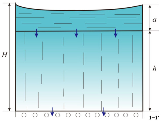
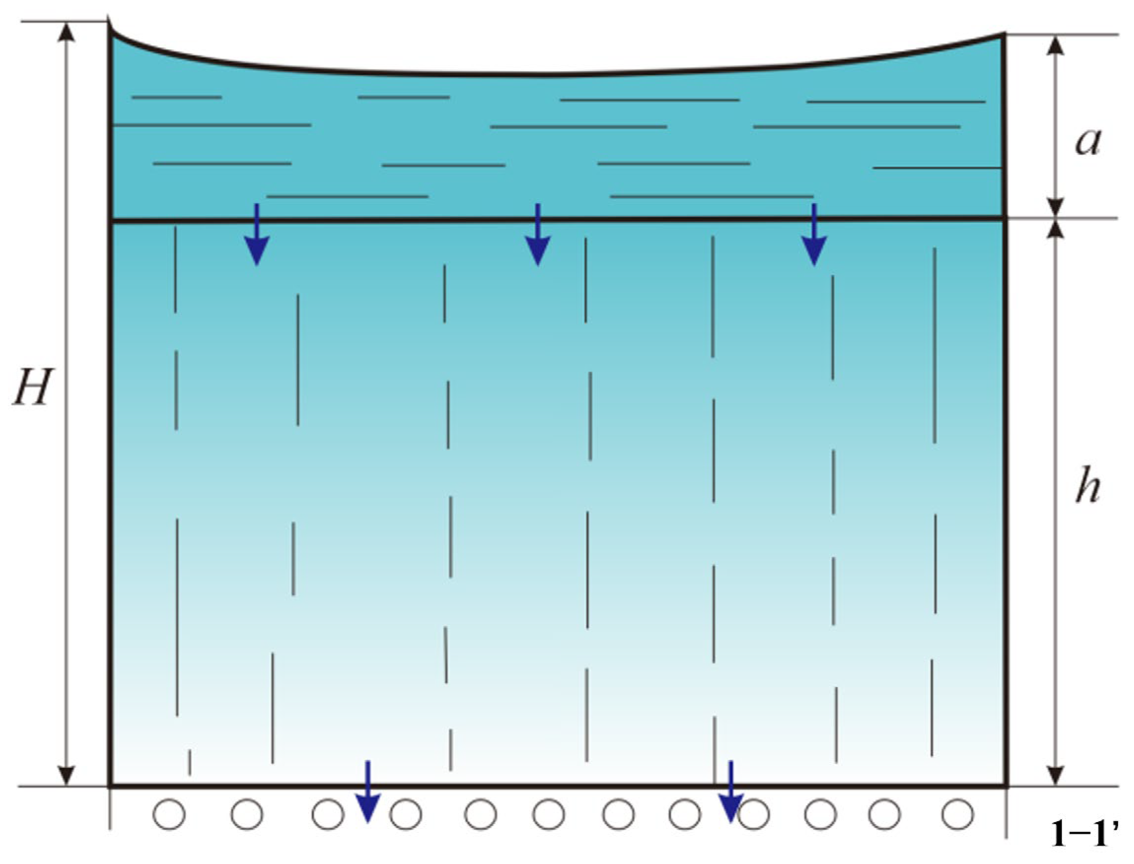
The Green-Ampt infiltration model was proposed by Green and Ampt in 1911 based on a constant water head [16]. The infiltration model is shown in Figure 2. Specifically, the upper part is water body in the height of a. Due to the gravity, the water shall flow downward. The soil body is uniform and isotropic, and the cross-sectional area of the soil is in unit one. It can be seen from the figure that the wetting front of the infiltration reaches the 1−1′ cross-section at this time. During the infiltration process, the soil will be divided into two parts by the wetting front. The soil in the upper part of the wetting front is saturated due to water infiltration, while the soil in the lower part of the wetting front is still in a natural state, where water content is the initial water content.

Figure 2. Schematic diagram of rainfall infiltration.

According to Darcy’s law,

$$i=K_s{\displaystyle \frac{h+a+S_f}{h}}$$

(8)

where i is the infiltration rate; S_f is the matrix suction of the wetting front at the 1-1′ section; a is the height of the water body; h is the water seepage path, that is, the distance between the top of the soil and the wetting front; K_s is the saturation permeability coefficient; h + a + S_f is the total water head.

Assuming that the moisture content inside the soil is uniformly distributed and equal to θ_i in the initial state, the moisture content in the saturated state is θ_s. Then the accumulated water infiltration amount in the soil is

$$I=({\theta }_s-{\theta }_i)h$$

(9)

Simplified,

$$i=K_s\left[1+{\displaystyle \frac{({\theta }_s-{\theta }_i)(S_f+a)}{I}}\right]$$

(10)

Set the difference of the moisture content as M = θ_s − θ_i. However, the total infiltration volume I and infiltration distance h are related to time t. Therefore, the derivation, integration, and simplification of Equation (9) can be obtained as follows:

$${\displaystyle \frac{dI}{dt}}=i=M{\displaystyle \frac{dh}{dt}}$$

(11)

$${\displaystyle \frac{dh}{dt}}={\displaystyle \frac{K_s}{M}}{\displaystyle \frac{h+a+S_f}{h}}$$

(12)

$${\displaystyle \int \frac{K_s}{M}}dt={\displaystyle \int \frac{h}{h+S_f+a}}dh$$

(13)

$${\displaystyle \frac{K_s}{M}}t=h-(a+S_f)\ln \left(1+{\displaystyle \frac{h}{S_f+a}}\right)$$

(14)

If S = a + S_f, the relationship between total infiltration volume I and time t can be obtained by combining Equations (6) and (11):

$$K_{s}t=I-SM\ln \left(1+{\displaystyle \frac{I}{SM}}\right)$$

(15)

According to Equations (14) and (15), the position of the wetting front and the total infiltration at any time can be obtained. However, this model can only be applied to the vertical infiltration of the horizontal plane; consequently, the Green-Ampt model shall be improved to make it suitable for rainfall infiltration of different slope shapes.

2.3. Rainfall Infiltration Law

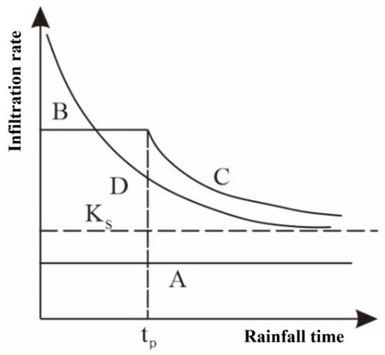
For the proposed Mein–Larson model [18], the regular curve of rainfall infiltration can be summarized as shown in Figure 3.

Figure 3. Curve of rainfall infiltration law.

Defining the rainfall intensity is p, the saturated permeability coefficient is K_s, and the soil water permeability is f_p.

Case A: Under the condition of low-intensity rainfall, p < K_s, all rainfall infiltrates without runoff, which is shown in curve A.

Case B: p < K_s < f_p, the rainfall intensity remains unchanged, the soil has a strong initial water permeability, and all rainfall penetrates the soil. In this case, the infiltration rate is equal to the unit rainfall, and the water level near the soil surface increases, which is the line segment B in the curve BC.

Case C: K_s < f_p ≤ p, with the infiltration of rainfall, the soil gradually becomes saturated, and the infiltration capacity decreases. When it is lower than the rainfall intensity, runoff occurs, and the time to start water accumulation is recorded as t_p, which is shown in curves C and D.

It is worth noting that most rainfall conditions may be rainfall infiltration with constant rainfall intensity in the water accumulation state, as shown in curve D, where t_s represents the time taken for the accumulated rainfall to reach I_p under the rainfall infiltration in the initial state of accumulation.

In short, based on the above-mentioned rainfall infiltration law, this paper explored the rainfall infiltration models of different slopes from two situations under constant rainfall conditions, namely, high-intensity rainfall (p > K_s) and low-intensity rainfall (p < K_s).

2.4. Rainfall Infiltration Models of Different Slope Shapes

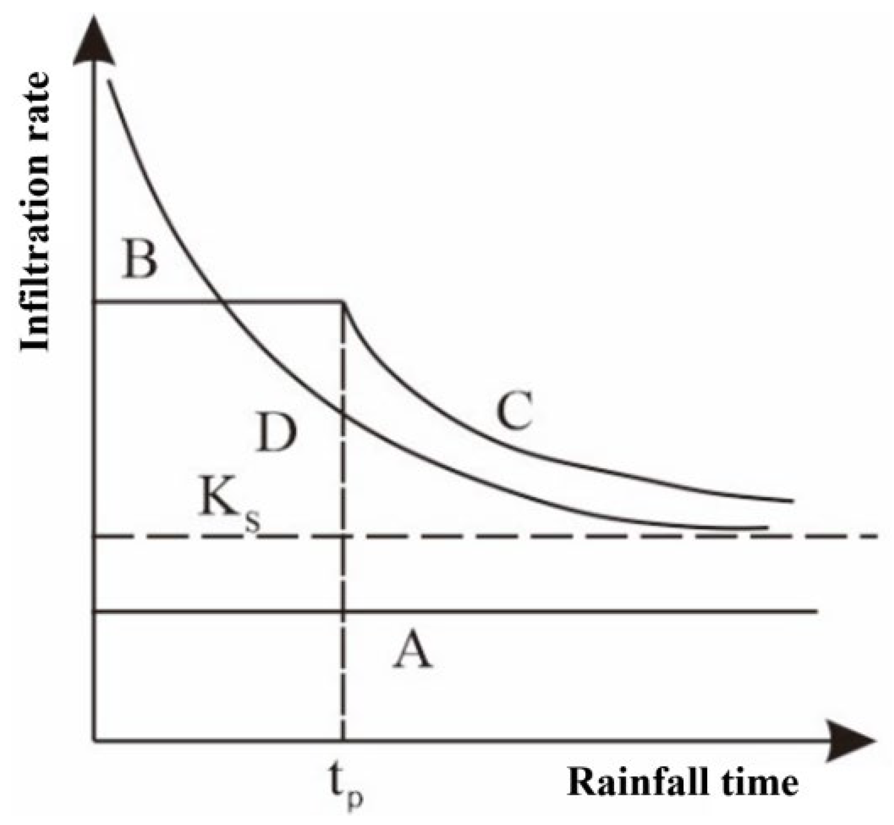
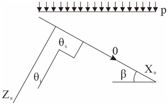
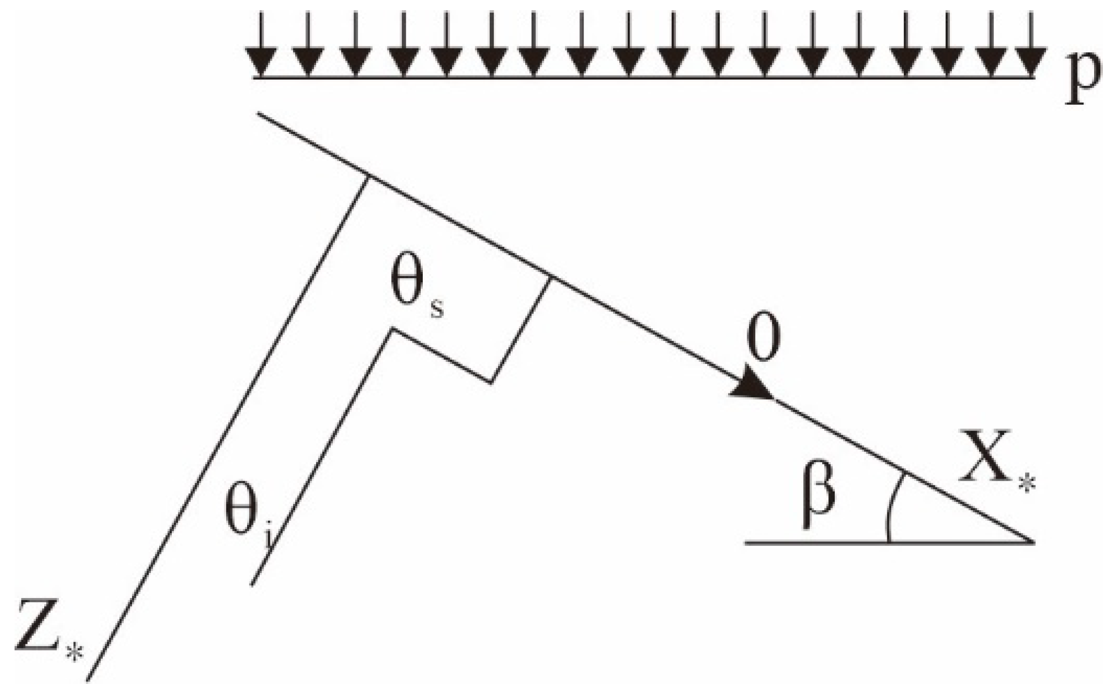
As substantiated from the definition of slope shape function, the main controlling factor for different slope shapes is the equivalent slope angle β. Therefore, regardless of the slope shape, the rainfall infiltration state of any point P(x,y) on the slope can be analyzed first, and the rainfall infiltration calculation diagram is portrayed in Figure 4.

Figure 4. Schematic diagram of rainfall infiltration model calculation (* indicates the direction of the coordinate axis).

Here, p is the rainfall intensity, and X_∗ and Z_∗ are the tangent direction of point P down the slope and the direction of the vertical tangent to the interior of the slope, respectively. θ_s is recorded as the saturated volumetric water content of the soil at point P; θ_i is recorded as the initial volumetric water content at point P; β is the equivalent slope angle of point P.

(1)

High-intensity rainfall (p > K_s)

When t is less than the water accumulation time t_p, that is, the line segment B in Figure 3, under this circumstance, the rainfall infiltration rate i is

$$i=p\cos \beta$$

(16)

Then, until the period of water accumulation, the cumulative infiltration amount I_p is

$$I_p={\displaystyle \frac{SM}{\frac{p\cos \beta }{K_s}-\cos \beta }}$$

(17)

Time t_p of this period is

$$t_p={\displaystyle \frac{SM}{\frac{p^2{\cos }^2\beta }{K_s}-p{\cos }^2\beta }}$$

(18)

When the time t is greater than the water accumulation time t_p, the rainfall infiltration law at this moment can be equivalently described by the curve D in Figure 3. Then, we let T = t − (t_p − t_s), and the time T represents the rain time when the initial state is the accumulation of water.

Applying Darcy’s law to the saturated zone above the wetting front, the infiltration rate i can be expressed as

$$i=K_s{\displaystyle \frac{Z_{\ast f}\cos \beta +S}{Z_{\ast f}}}$$

(19)

where Z_∗f is the depth of the wetting front measured along the Z_∗-axis (normal to the slope), Z_∗fcosβ represents the gravitational head at the wetting front, and S is the average matrix suction head at the wetting front [16,18]. This equation reflects the physical principle that the infiltration rate is controlled by the hydraulic gradient across the saturated zone.

Defining the water content deficit M = θ_s − θ_i, the cumulative infiltration I at time T is related to the wetting front depth by

$$I=M{Z}_{\ast f}$$

(20)

Deriving Equation (20),

$${\displaystyle \frac{dI}{dT}}=i=M{\displaystyle \frac{d{Z}_{\ast f}}{dT}}$$

(21)

Simultaneously, Equation (19) is

$${\displaystyle \frac{d{Z}_{\ast f}}{dT}}={\displaystyle \frac{K_s}{M}}{\displaystyle \frac{Z_{\ast f}\cos \beta +S}{Z_{\ast f}}}$$

(22)

Equation (22) is a differential equation describing the evolution of cumulative infiltration with time under ponded conditions. Integrating Equation (22),

$${\displaystyle \int \frac{K_s}{M}}dT={\displaystyle \int \frac{Z_{\ast f}}{Z_{\ast f}\cos \beta +S}}d{Z}_{\ast f}$$

(23)

Further simplified,

$$K_{s}T\cos \beta =I-{\displaystyle \frac{SM}{\cos \beta }}\ln \left(1+{\displaystyle \frac{I\cos \beta }{SM}}\right)$$

(24)

Equation (24) is the implicit Green-Ampt infiltration equation adapted for sloping surfaces, where the gravitational term appears through the relationship between Z_∗f and I in Equation (20), and the slope angle β influences the conversion between normal depth and vertical depth when needed.

At the moment ponding begins (t = t_p), the cumulative infiltration is I_p. The corresponding shifted time t_s (the time required to reach I_p under ponded conditions) can be obtained from Equation (24) by setting I = I_p and solving for T = t_s:

$$t_s=\left[I_p-{\displaystyle \frac{SM}{\cos \beta }}\ln \left(1+{\displaystyle \frac{I_p\cos \beta }{SM}}\right)\right]/K_s\cos \beta$$

(25)

where t_s is the time required when the initial rainfall condition is accumulated water and the total infiltration amount I = I_p.

In summary, it is reasonable to submit that the penetration depth of the wetting front in the Z_∗ direction at any time can be expressed as

$$\left\{\begin{array}{cc}{Z}_{\ast f}={\displaystyle \frac{pt\cos \beta }{M}}\hspace{1em}\hspace{1em}& t\le t_p\\ K_s\left[t-\left(t_p-t_s\right)\right]={\displaystyle \frac{1}{\cos \beta }}\left[Z_{\ast f}-{\displaystyle \frac{S}{\cos \beta }}\ln \left({\displaystyle \frac{Z_{\ast f}\cos \beta +S}{S}}\right)\right]& t>t_p\end{array}\hspace{1em}\hspace{1em}\right.$$

(26)

Equation (26) provides a complete description of wetting front advancement under high-intensity rainfall, accounting for both the pre-ponding and post-ponding phases.

(2)

Low-intensity rainfall (p < K_s)

When rainfall intensity is lower than the saturated permeability(p < K_s), no ponding occurs and all rainfall infiltrates. In this case, the infiltration rate equals the rainfall intensity throughout the process, and the cumulative infiltration increases linearly with time:

$$I=p\mathrm{tcos}\beta$$

(27)

Using the relationship between cumulative infiltration and wetting front depth (Equation (20)), the wetting front depth along the Z_∗-direction is

$$Z_{\ast f}={\displaystyle \frac{pt\cos \beta }{M}}$$

(28)

Equations (27) and (28) represent the simplest form of the infiltration model under low-intensity rainfall, where the wetting front advances at a constant rate determined by the rainfall intensity and the soil’s water content deficit.

Furthermore, the equivalent slope angle β and the depth of the wetting front at point P shall also change with the position of point P. Additionally, when a certain infiltration point on the slope is determined, the depth of its wetting front is also uniquely determined. Therefore, for a slope with any slope shape, the infiltration depth of the wetting front at each point of the slope can be obtained by the above model according to the two kinds of rainfall conditions; that is, the change law of the wetting front with time can be obtained to explore the law of rainfall infiltration on different slopes. The local slope angle β influences infiltration depth through two mechanisms: (1) the gravitational head term Z_∗f cosβ in Equation (19), which affects the infiltration rate; (2) the conversion from normal depth Z_∗f to vertical depth Z_w = Z_∗f/cosβ used in stability calculations. As a result, for the same normal infiltration depth, convex slopes (smaller cosβ near the toe) yield larger vertical depths, accelerating failure.

3. Stability Model of Different Slope Shapes

The stability calculation method in this paper makes the following assumptions: (1) the soil in the slope is an isotropic homogeneous body; (2) there is no accumulated water on the surface, which means the surface water head H = 0.

3.1. Infiltration Modeling Framework

The infiltration analysis in this study considers two distinct rainfall regimes with different boundary conditions. For high-intensity rainfall, the rainfall intensity exceeds the soil’s infiltration capacity. Initially, all rainfall infiltrates (flux-controlled boundary). Once the surface becomes saturated at ponding time tp, the boundary condition switches to head-controlled (zero pressure head at the surface), and runoff may occur. For low-intensity rainfall, rainfall intensity is less than the saturated hydraulic conductivity. All rainfall infiltrates throughout the event, and the surface never reaches saturation. The boundary remains flux-controlled, with infiltration rate equal to rainfall intensity throughout.

3.2. Linear Slope Model

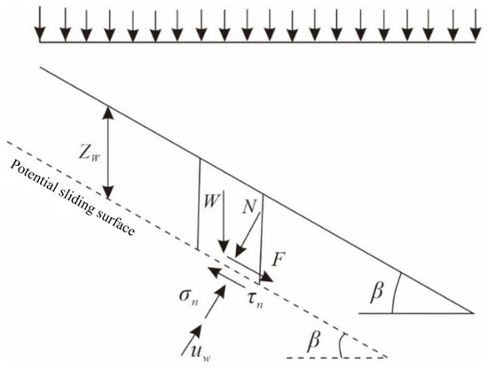
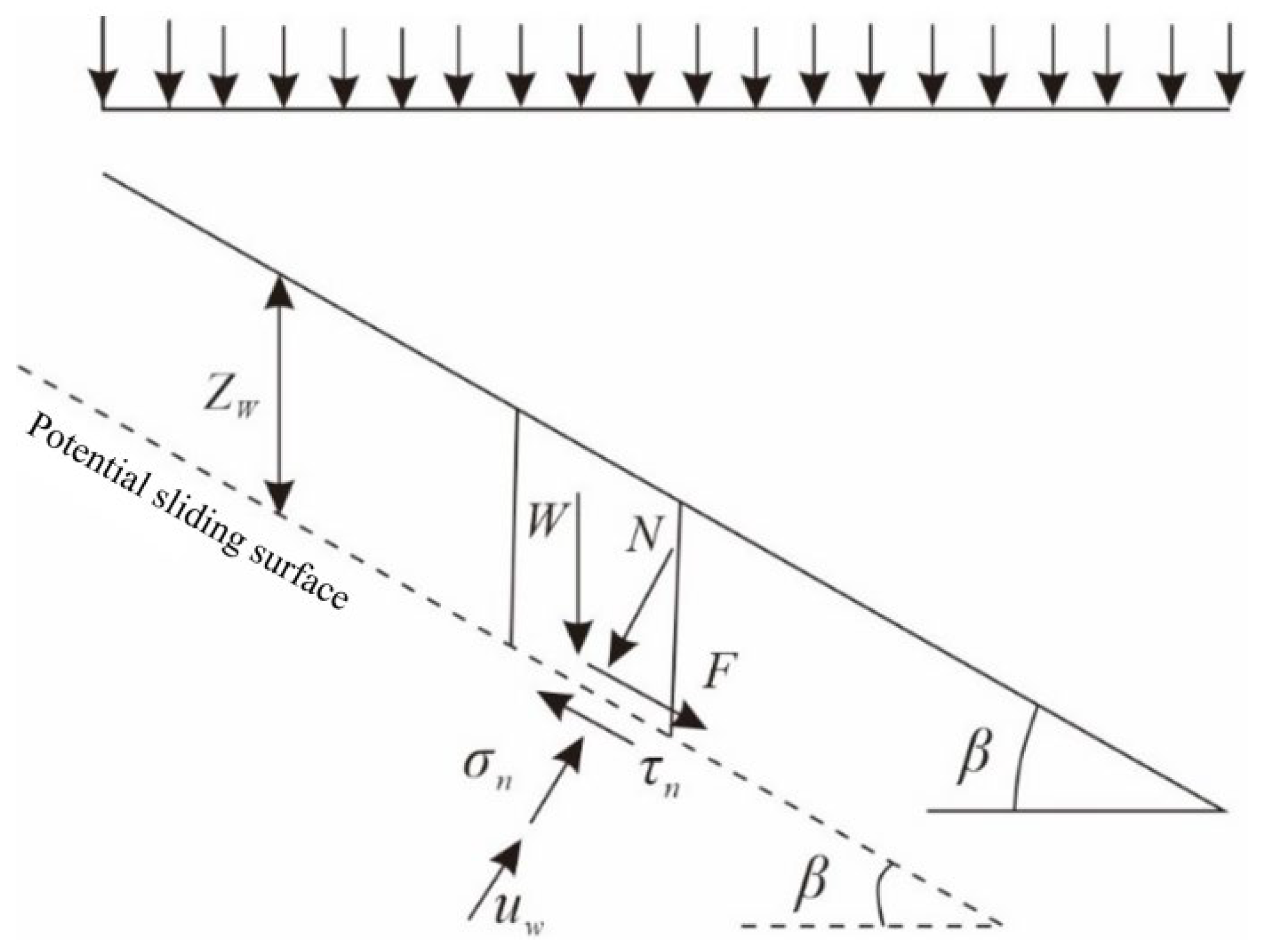
Linear slope can usually be regarded as an infinite slope. Thus, we take any element of the slope for stability analysis. The stability calculation model is shown in Figure 5.

Figure 5. Schematic diagram of linear slope stability calculation.

Where Z_W is the vertical infiltration depth of the wetting front, and Z_W = Z_∗f/cosβ, the slope angle is β, and the relevant parameters at the potential sliding surface are assumed to be normal stress σ_n, shear stress τ_n, pore pressure u_w. The soil state from top to bottom of the wetting front is saturated and natural, respectively.

Then, the gravity of the unit body is

$$W={\gamma }_{sat}{Z}_W$$

(29)

In Equation (29), γ_sat is the saturation weight of the soil, and other parameters are the same as above.

Decomposing gravity along the slope direction and perpendicular to the slope direction, thus, the normal stress N and the sliding force F can be written as

$$N=W\cos \beta ={\gamma }_{sat}{Z}_W\cos \beta$$

(30)

$$F=W\sin \beta ={\gamma }_{sat}{Z}_W\sin \beta$$

(31)

Considering the effective surface area of the unit body S = 1/cosβ, therefore, the total normal stress σ_n on the potential sliding surface is

$${\sigma }_n=N/{\displaystyle \frac{1}{\cos \beta }}={\gamma }_{sat}{Z}_W{\cos }^2\beta$$

(32)

Furthermore, the shear stress τ_n on the potential sliding surface is

$${\tau }_n=F/{\displaystyle \frac{1}{\cos \beta }}={\gamma }_{sat}{Z}_W\sin \beta \cos \beta$$

(33)

Mohr–Coulomb formula:

$$\tau =c+\sigma \tan \phi$$

(34)

Therefore, the shear strength τ of the unit body is

$$\tau =c\prime +\sigma \tan \phi \prime =c\prime +({\sigma }_n-u_w)\tan \phi \prime$$

(35)

In Equation (35), c′, φ′ are the cohesion and internal friction angle in the saturated state, respectively. Other parameters are the same as above.

The factor of safety of the slope is

$$F_{Sz}={\displaystyle \frac{\tau }{{\tau }_n}}={\displaystyle \frac{c\prime +({\sigma }_n-u_w)\tan \phi \prime }{{\gamma }_{sat}{Z}_W\sin \beta \cos \beta }}$$

(36)

In Equation (36), we introduce the F_Sz to represent the factor of safety of the linear slope, and other parameters are the same as above.

If the infiltration depth of the wetting front is less than the depth of the bedrock, the pore water pressure (u_w) remains constant, and u_w = −Sγ_w, where S is the equivalent head of the matrix suction at the wetting front. Accordingly, the factor of safety of the slope is

$${F_S}_z={\displaystyle \frac{\tau }{{\tau }_n}}={\displaystyle \frac{c\prime +({\gamma }_{sat}{Z}_W{\cos }^2\beta +S{\gamma }_w)\tan \phi \prime }{{\gamma }_{sat}{Z}_W\sin \beta \cos \beta }}$$

(37)

(1)

High-intensity rainfall (p > K_s)

The vertical infiltration depth Z_W of the wetting front in each period is

$$\left\{\begin{array}{ll}{Z}_W={\displaystyle \frac{pt}{M}}\hspace{1em}\hspace{1em}& t\le t_p\\ Z_W={\displaystyle \frac{I}{M\cos \beta }}& t>t_p\end{array}\hspace{1em}\hspace{1em}\right.$$

(38)

Especially, when the rainfall time is determined, the vertical wetting front infiltration depth Z_W of the linear slope can be obtained. Therefore, the stability under the condition of high-intensity rainfall is

$$\left\{\begin{array}{cc}{F_S}_z={\displaystyle \frac{\tan \phi \prime }{\tan \beta }}+{\displaystyle \frac{(c\prime +S{\gamma }_w\tan \phi \prime )M}{{\gamma }_{sat}pt\sin \beta \cos \beta }}& t\le t_p\\ {F_S}_z={\displaystyle \frac{\tan \phi \prime }{\tan \beta }}+{\displaystyle \frac{(c\prime +S{\gamma }_w\tan \phi \prime )M}{{\gamma }_{sat}I\sin \beta }}& t>t_p\end{array}\hspace{1em}\hspace{1em}\right.$$

(39)

where M is the difference in water content, p is the rainfall intensity, and I is the cumulative infiltration.

(2)

Low-intensity rainfall (p < K_s)

The vertical infiltration depth Z_W of the wetting front under low rainfall intensity is

$$Z_W={\displaystyle \frac{pt}{M}}$$

(40)

Similarly, when the rainfall time is determined, the wetting front infiltration depth Z_W in the vertical direction of the linear slope can be obtained. Thus, the stability under the condition of low rainfall can be expressed as

$${F_S}_z={\displaystyle \frac{\tan \phi \prime }{\tan \beta }}+{\displaystyle \frac{(c\prime +S{\gamma }_w\tan \phi \prime )M}{{\gamma }_{sat}pt\sin \beta \cos \beta }}$$

(41)

3.3. Concave Slope Model

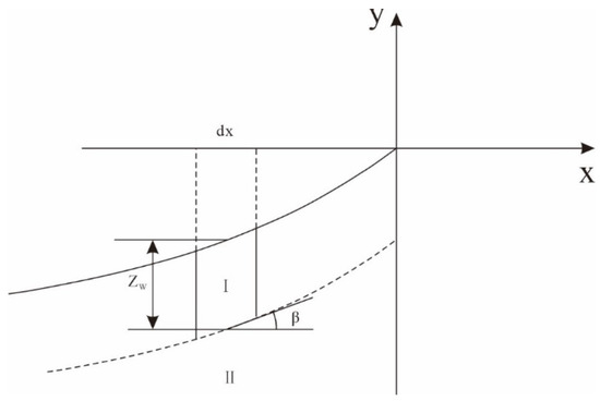
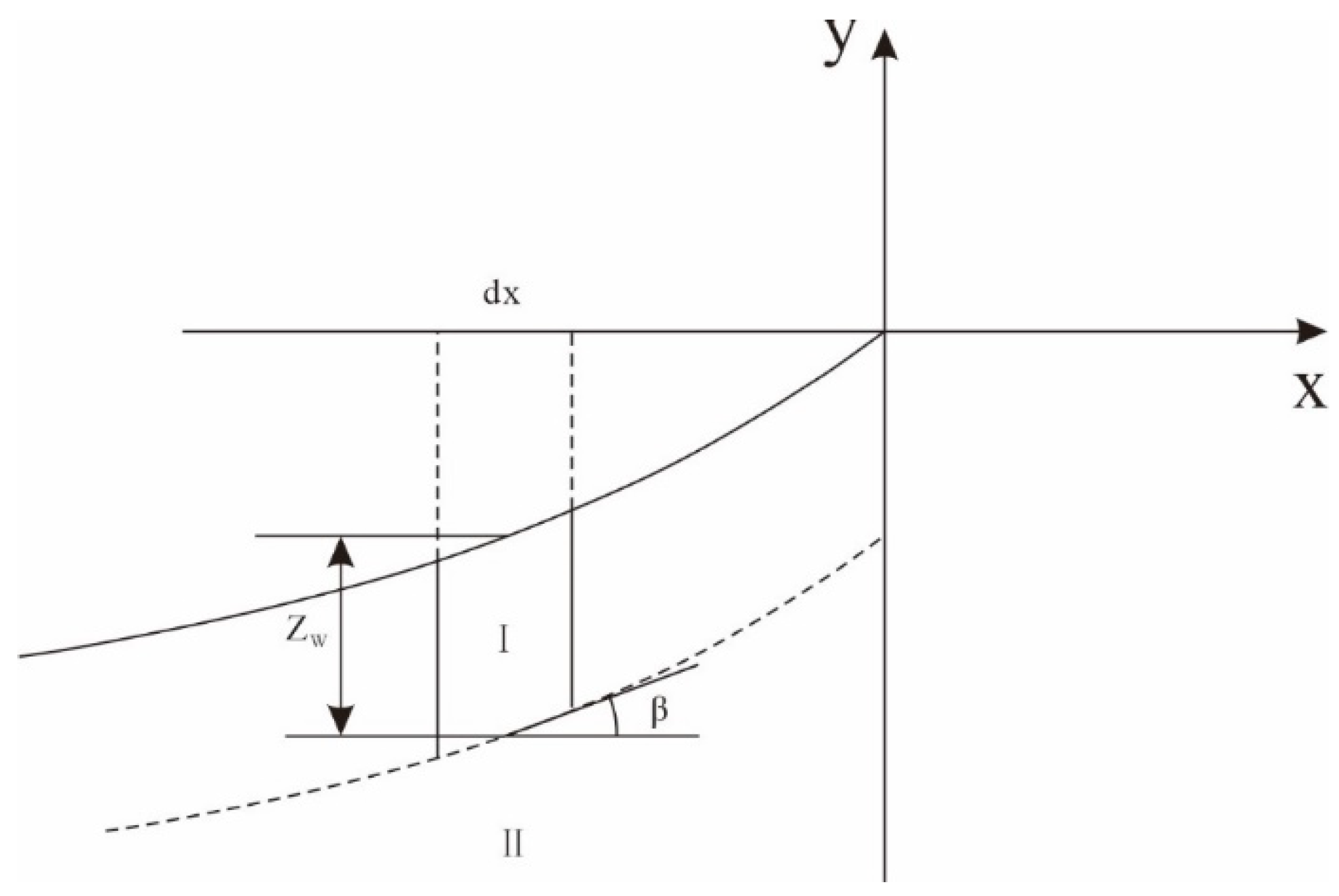
Owing to its homogeneity and isotropy, the wetting front infiltration depth of the concave slope soil is parallel to the slope surface; then, it is reasonable to assume that the wetting front is the potential sliding surface of the concave slope. As shown in Figure 6, the slope is equally divided into n blocks with a spacing of dx. In addition, the part above the wetting front is zone I, while the part below the wetting front is zone II. Notably, the slope in zone I is already in a fully saturated state, thus, the buoyant unit weight γ′ is employed for calculation, while natural unit weight γ_t is taken for the slope in zone II, which is still in a natural state.

Figure 6. Schematic diagram of stability calculation of concave slope.

As for the calculation of factor of safety, the vertical infiltration depth of a wetting front on any slope, alternatively, the average value of the vertical infiltration depth at both ends of the wetting front, is recorded as Z_W, and the average value of the equivalent slope angle at both ends of the wetting front is denoted as β.

Therefore, we can perform a mechanical analysis on the block, and the gravity dW₁ of the block in Zone I can be obtained by Equation (42):

$$d{W}_1={\gamma }^{\prime }{Z}_{W}dx$$

(42)

Decomposing gravity along the tangent direction of the block and perpendicular to the tangent direction of the block, the normal stress dN and the sliding force dF are

$$dN=d{W}_1\cos \beta ={\gamma }^{\prime }{Z}_W\cos \beta dx$$

(43)

$$dF=d{W}_1\sin \beta ={\gamma }^{\prime }{Z}_W\sin \beta dx$$

(44)

According to the Mohr–Coulomb formula, the sliding resistance dR of the slope can be obtained as

$$dR=d{W}_1\cos \beta \tan \phi \prime +c\prime {\displaystyle \frac{dx}{\cos \beta }}=(\gamma \prime Z_W\cos \beta \tan \phi \prime +{\displaystyle \frac{c\prime }{\cos \beta }})dx$$

(45)

where c′, φ′ are the cohesion and internal friction angle in the saturated state, respectively, and other parameters are the same as above.

From the definition of unit permeability,

$$J={\gamma }_{w}i$$

(46)

Here, J represents the permeability of saturated soil, γ_w is the weight of water, and i is the water potential gradient.

Since the block is so small that the change in the equivalent slope angle β can be ignored, we can approximate cosβ ≈ 1. Furthermore, the water potential gradient i of the block is

$$i=\tan \beta =\sin \beta$$

(47)

So that

$$dJ={\gamma }_w{S}_{k}i={\gamma }_w{Z}_{W}dx\sin \beta$$

(48)

where S_k is the area of the block, and other parameters have the same meaning as above.

Therefore, the anti-sliding force, penetration force, and sliding force of the block can be obtained by summing the blocks, which are

$$R={\displaystyle \sum _1^{n}d}R\hspace{1em}$$

(49)

$$J={\displaystyle \sum _1^{n}d}J$$

(50)

$$F={\displaystyle \sum _1^{n}d}F\hspace{1em}$$

(51)

If there is shallow failure at the wetting front of the concave slope, the stability calculation formula at the wetting front is changed to

$$F_{Sa}={\displaystyle \frac{R}{F+J}}$$

(52)

where F_sa is the factor of safety of the concave slope, and the expansion is

$$F_{Sa}={\displaystyle \sum _1^n\frac{\gamma \prime Z_W{\cos }^2\beta \tan \phi \prime +c\prime }{{\gamma }_{sat}{Z}_W\sin \beta \cos \beta }}={\displaystyle \sum _1^n(\frac{\gamma \prime \tan \phi \prime }{{\gamma }_{sat}\tan \beta }+\frac{c\prime }{{\gamma }_{sat}{Z}_W\sin \beta \cos \beta })}$$

(53)

In Equation (53), γ_sat is the saturation weight of the soil, and γ_sat = γ_w + γ′. The meaning of other parameters is the same as above. Physically, the higher stability of concave slopes arises from the “buttressing effect”: as β increases towards the toe, the normal stress on the potential sliding surface increases, enhancing frictional resistance. This is captured in Equation (53) through the integration of cosβ terms.

(1)

High-intensity rainfall (p > K_s)

If the rainfall time is determined, the vertical wetting front infiltration depth Z_W of the concave slope can be obtained. Therefore, the factor of safety of the concave slope under the condition of high-intensity rainfall is

$$\left\{\begin{array}{ll}{F_S}_a={\displaystyle \sum _1^n(\frac{\gamma \prime \tan \phi \prime }{{\gamma }_{sat}\tan \beta }+\frac{Mc\prime }{{\gamma }_{sat}pt\sin \beta \cos \beta })}\hspace{1em}& t\le t_p\\ \hspace{1em}{F_S}_a={\displaystyle \sum _1^n(\frac{\gamma \prime \tan \phi \prime }{{\gamma }_{sat}\tan \beta }+\frac{Mc\prime }{{\gamma }_{sat}I\sin \beta })}& t>t_p\end{array}\hspace{1em}\hspace{1em}\right.$$

(54)

where M is the difference in water content, p is the rainfall intensity, and I is the cumulative infiltration.

(2)

Low-intensity rainfall (p < K_s)

Like the former, when the rainfall time is determined, the vertical wetting front infiltration depth Z_W of the concave slope can also be obtained. Therefore, the factor of safety of the concave slope under the condition of low rainfall can be expressed as

$${F_S}_a={\displaystyle \sum _1^n(\frac{\gamma \prime \tan \phi \prime }{{\gamma }_{sat}\tan \beta }+\frac{Mc\prime }{{\gamma }_{sat}pt\sin \beta \cos \beta })}\hspace{1em}$$

(55)

3.4. Convex Slope Model

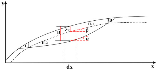
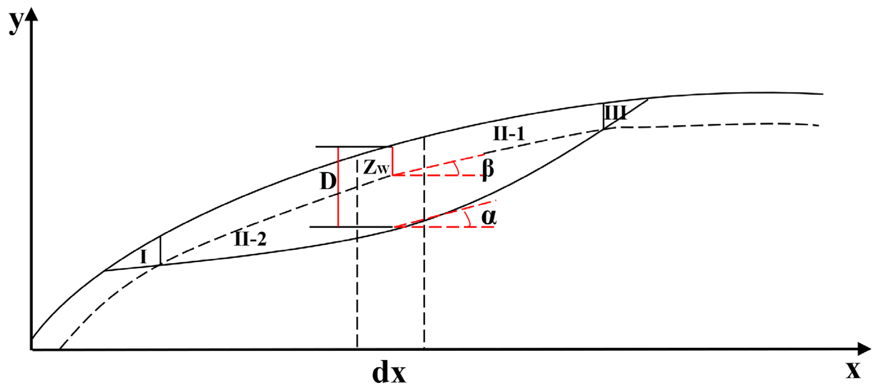
The infiltration depth of the wetting front of the isotropic homogeneous convex slope is parallel to the slope. In addition, the slopes tend to rupture in the shapes of arcs or concave lines. The convex slope calculation model is shown in Figure 7. Like the method for concave slopes, to obtain the factor of safety of convex slopes under two constant rainfall conditions, we divide the slopes into three areas, in which the soils in zones I and III are saturated, and the soil in Zone II-1 is saturated, and the soil in Zone II-2 is in a natural state. Moreover, the buoyant unit weight γ′ is employed for the calculation of saturated soil, while natural unit weight γ_t is applied for the slope that is still in a natural state.

Figure 7. Schematic diagram of stability calculation of convex slope.

The three parts are divided into n blocks, and the spacing of each block is dx.

When calculating the factor of safety of the slope, we can use the average value of the vertical infiltration depth at both ends of the wetting front to replace the vertical infiltration depth of the wetting front at any slope, which is recorded as Z_W. The thickness of the slope is D, and D = F(x) − R(x). The average values of the equivalent slope angles at both ends of the potential sliding surface and the wetting front are denoted as α and β, respectively.

The gravity levels of the blocks in zone I and zone III are

$$d{W}_1=d{W}_3=\gamma \prime Ddx$$

(56)

where γ′ is the buoyant unit weight of the soil.

The gravity is decomposed along the tangent direction of the potential sliding surface and the tangent direction perpendicular to the sliding surface, and the normal stress dN₁, dN₃ and sliding force dF₁, dF₃ can be obtained as follows:

$$d{N}_1=d{N}_3=\gamma \prime D\cos \alpha dx$$

(57)

$$d{F}_1=d{F}_3=\gamma \prime D\sin \alpha dx$$

(58)

According to the Mohr–Coulomb formula,

$$d{R}_1=d{R}_3=\gamma \prime D\cos \alpha \tan \phi \prime dx+c\prime {\displaystyle \frac{dx}{\cos \alpha }}$$

(59)

where c′, φ′ are the cohesion and internal friction angle in the saturated state, respectively, and other parameters have the same meaning as above.

From the previous analysis on the permeability of the concave slope, the permeability dJ₁ and dJ₃ of the block can be expressed as follows:

$$d{J}_1=d{J}_3={\gamma }_w{S}_{k}i={\gamma }_{w}Ddx\sin \alpha$$

(60)

where S_k is the area of the block, γ_w is the weight of water, and i is the water potential gradient. The meaning of other parameters is the same as above.

Then, the gravity dW₂₁ of the block in the Zone II-1 is

$$d{W}_{21}=\gamma \prime Z_{W}dx$$

(61)

Furthermore, the gravity dW₂₂ of block in the Zone II-2 is

$$d{W}_{22}={\gamma }_t(D-Z_W)dx$$

(62)

In Equations (61) and (62), γ_t is the natural gravity of the soil, and other parameters have the same meaning as above.

Decomposing the gravity along the tangent direction of the potential sliding surface and the tangent direction perpendicular to the sliding surface, the normal stress dN₂ and sliding force dF₂ can be obtained as follows:

$$d{N}_2=(d{W}_{21}+d{W}_{22})\cos \alpha =(\gamma \prime Z_W+{\gamma }_t(D-Z_W))\cos \alpha dx$$

(63)

$$d{F}_2=(d{W}_{21}+d{W}_{22})\sin \alpha =(\gamma \prime Z_W+{\gamma }_t(D-Z_W))\sin \alpha dx$$

(64)

From the Mohr–Coulomb formula,

$$d{R}_2=(d{W}_{21}+d{W}_{22})\cos \alpha \tan \phi +c{\displaystyle \frac{dx}{\cos \alpha }}$$

(65)

$$d{R}_2=\left[({\gamma }^{\prime }{Z}_W+{\gamma }_t(D-Z_W))\cos \alpha \tan \phi +{\displaystyle \frac{c}{\cos \alpha }}\right]dx$$

(66)

where c, φ are, respectively, the cohesion and internal friction angle in the natural state, and other parameters are the same as above.

From the previous analysis on the permeability of the concave slope, the permeability dJ₂ of the block can be expressed as

$$d{J}_2={\gamma }_w{S}_{k}i={\gamma }_w{Z}_{W}dx\sin \beta$$

(67)

Therefore, the anti-sliding force, penetration force, and sliding force of the block can be obtained by summing the blocks, which are

$$R={\displaystyle \sum _1^{n}d}R\hspace{1em}$$

(68)

$$J={\displaystyle \sum _1^{n}d}J$$

(69)

$$F={\displaystyle \sum _1^{n}d}F\hspace{1em}$$

(70)

The factor of safety at the potential sliding surface of the convex slope is

$$F_{St}={\displaystyle \frac{R}{F+J}}$$

(71)

where F_st is the factor of safety of the convex slope, and the expansion is

$$F_{st}={\displaystyle \sum _1^n\frac{\left[(\gamma \prime Z_W+{\gamma }_t(D-Z_W))\tan \phi +2\gamma \prime D\tan {\phi }^{\prime }\right]{\cos }^2\alpha +2c\prime +c}{\left[Z_W\sin \beta +2D\sin \alpha \right]{\gamma }_w\cos \alpha +\left[\gamma \prime Z_W+{\gamma }_t(D-Z_W)+2\gamma \prime D\right]\sin \alpha \cos \alpha }}$$

(72)

For convex slopes, the decreasing β towards the toe concentrates shear stress and accelerates pore pressure buildup, reducing stability. This stress concentration is mathematically reflected in Equation (72), where the varying β modifies the driving force integral.

(1)

High-intensity rainfall (p > K_s)

When the rainfall time is determined, the vertical wetting front infiltration depth Z_W of the convex-line slope can be obtained as well. Therefore, the factor of safety of the convex slope under the condition of high-intensity rainfall is as follows:

$$\left\{\begin{array}{cc}{F}_{St}={\displaystyle \sum _1^n\frac{\left[(\gamma \prime pt+{\gamma }_t(DM-pt))\tan \phi +2\gamma \prime DM\tan \phi \prime \right]{\cos }^2\alpha +(2c\prime +c)M}{\left[pt\sin \beta +2DM\sin \alpha \right]{\gamma }_w\cos \alpha +\left[\gamma \prime pt+{\gamma }_t(DM-pt)+2\gamma \prime DM\right]\sin \alpha \cos \alpha }}& t\le t_p\\ F_{St}={\displaystyle \sum _1^n\frac{\left[(\gamma \prime I+{\gamma }_t(DM\cos \beta -I))\tan \phi +2\gamma \prime DM\cos \beta \tan \phi \prime \right]{\cos }^2\alpha +(2c\prime +c)M\cos \beta }{\left[I\sin \beta +2DM\cos \beta \sin \alpha \right]{\gamma }_w\cos \alpha +\left[\gamma \prime I+{\gamma }_t(DM\cos \beta -I)+2\gamma \prime DM\cos \beta \right]\sin \alpha \cos \alpha }}& t>t_p\end{array}\right.$$

(73)

where M is the difference in water content, p is the rainfall intensity, and I is the cumulative infiltration.

(2)

Low-intensity rainfall (p < K_s)

Like the former, if the rainfall time is determined, the vertical wetting front infiltration depth Z_W of the concave slope can also be obtained. Thus, the factor of safety of the concave slope under the condition of low rainfall can be expressed as

$$F_{St}={\displaystyle \sum _1^n\frac{\left[(\gamma \prime pt+{\gamma }_t(DM-pt))\tan \phi +2\gamma \prime DM\tan \phi \prime \right]{\cos }^2\alpha +(2c\prime +c)M}{\left[pt\sin \beta +2DM\sin \alpha \right]{\gamma }_w\cos \alpha +\left[\gamma \prime pt+{\gamma }_t(DM-pt)+2\gamma \prime DM\right]\sin \alpha \cos \alpha }}$$

(74)

4. Case Study

Based on the above theoretical analysis, this paper takes a loess slope as an example to conduct slope stability calculation and numerical simulation analysis under rainfall conditions. The physical parameters of the loess slope are shown in Table 1. The calculation of slope stability is realized on MATLAB 2019a, and the numerical simulation is based on GeoStudio 2018 software. Moreover, the slope stability calculation and numerical simulation analysis are conducted to simulate the distribution law of the wetting front of different slopes under high- and low-intensity rainfall. Additionally, for the convenience of distinguishing, the intensities of two types of rainfall are set as p = 85 mm/d and 20 mm/d, respectively.

Table 1. Slope geotechnical and hydrological parameter.

Parameter	Saturated Cohesion (kPa)	Saturated Internal Friction Angle (°)	Natural Cohesion (kPa)	Natural Internal Friction Angle (°)	Natural Unit Weight (kN·m−3)	Saturated Unit Weight (kN·m−3)	Saturated Permeability Coefficient (m·d−1)
Loess	23	18	32	24.6	18	21	0.075

The geotechnical and hydrological parameters presented in Table 1 are not arbitrarily assigned but are derived from typical ranges reported in established experimental studies on loess soils from the Loess Plateau region of Northwest China [44,45,46]. Specifically, the saturated cohesion (23 kPa) and internal friction angle (18°), the natural cohesion (32 kPa) and friction angle (24.6°), the natural unit weight (18 kN/m³), the saturated unit weight (21 kN/m³), and the saturated permeability coefficient (0.075 m/d) fall within the commonly observed ranges for loess materials. These values are representative of the basic mechanical and hydraulic behavior of loess and are adequate for demonstrating the performance of the theoretical models proposed in this study. It is important to note, however, that for practical engineering applications at specific sites, parameters should be calibrated using site-specific laboratory or in situ tests to ensure accurate stability assessments.

4.1. Linear Slope Model

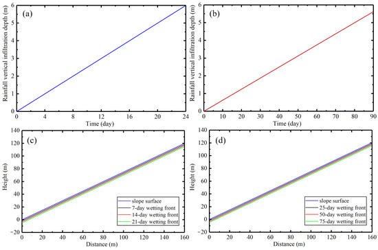
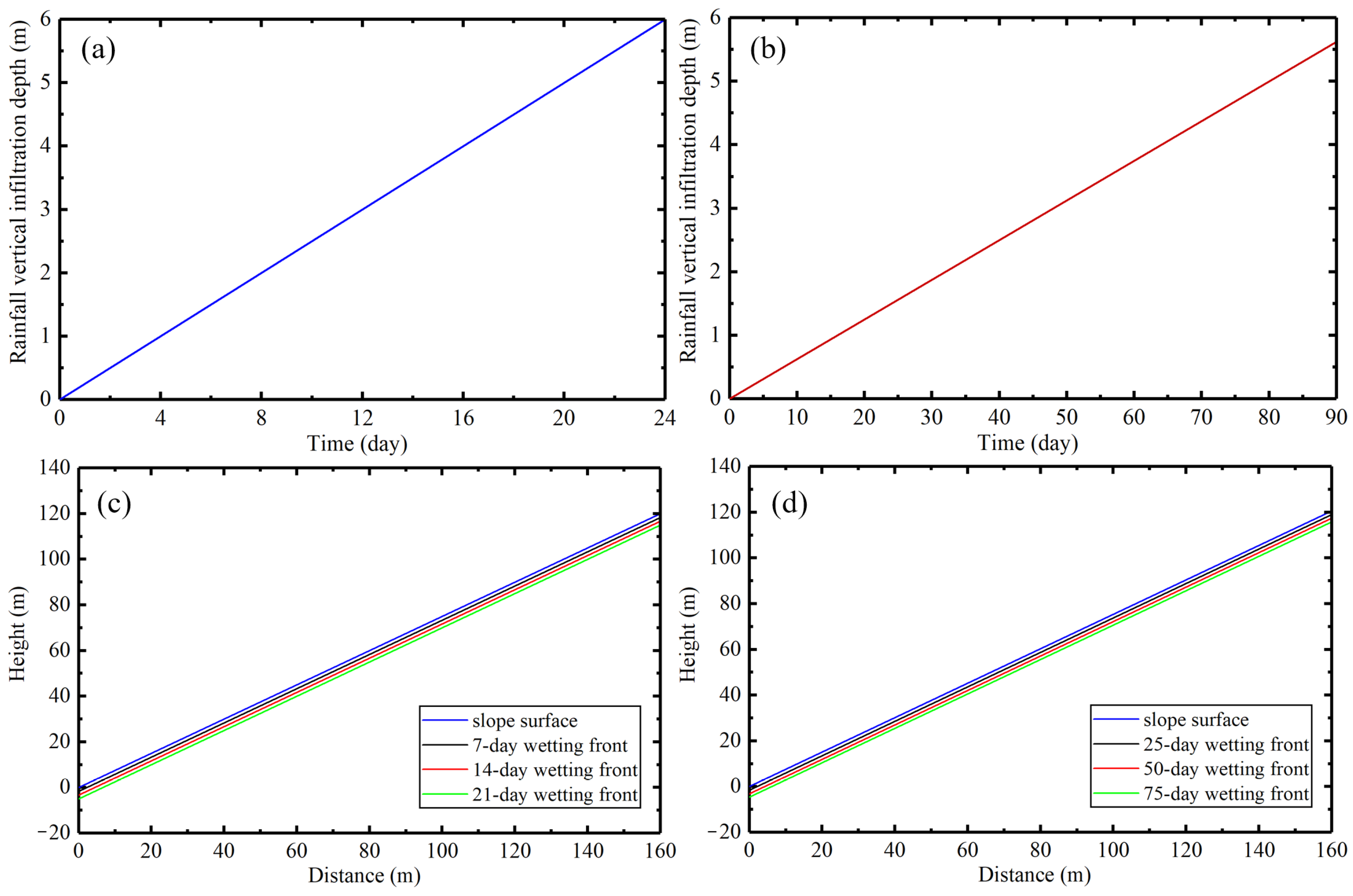
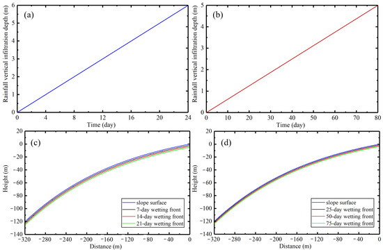
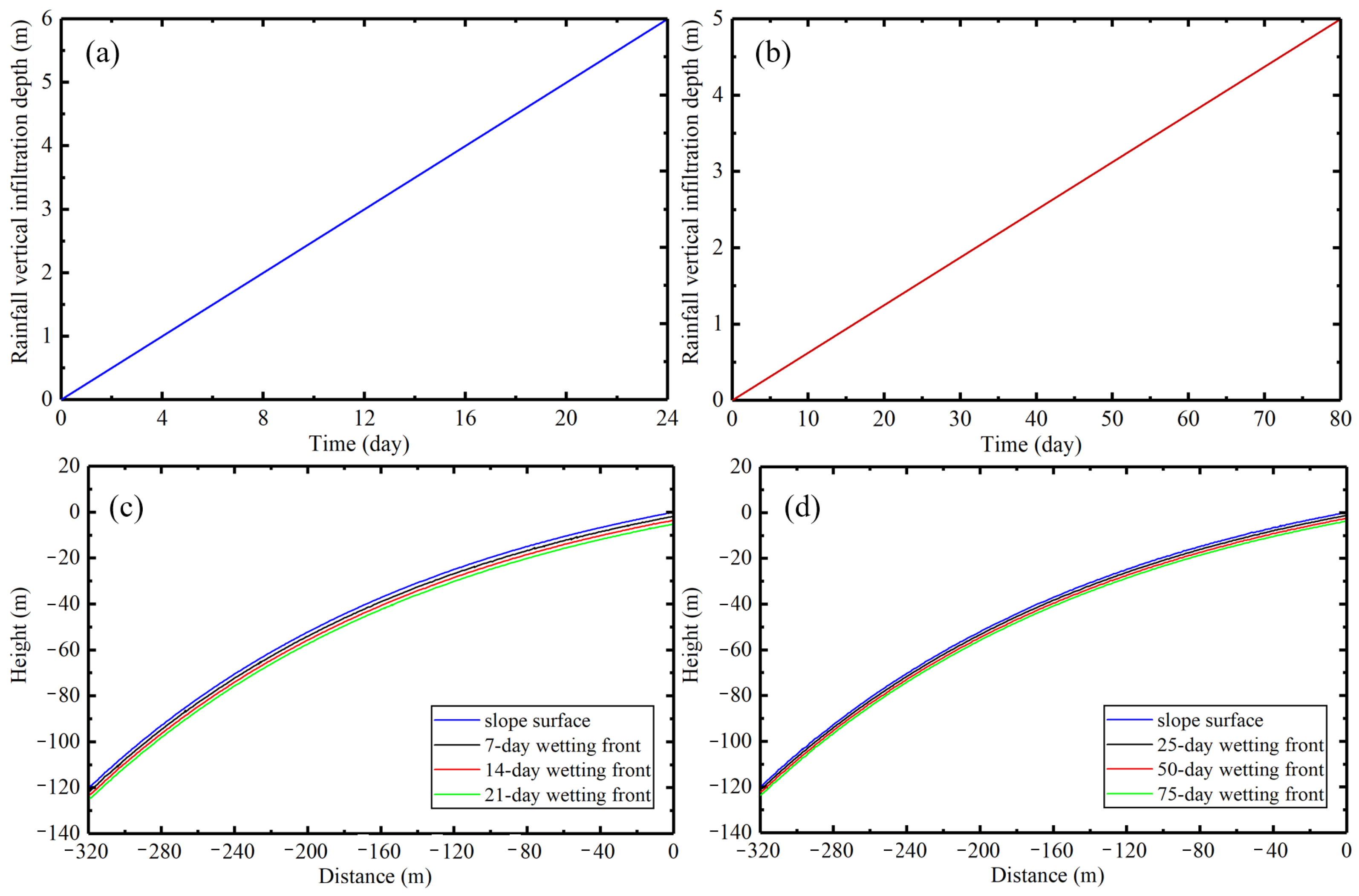
Under the condition of high-intensity rainfall (p = 85 mm/d, p > K_s), the rainfall infiltration of the linear slope is shown in Figure 8a. The vertical infiltration depth of the wetting front increases linearly with rainfall time, reaching the maximum infiltration depth of 5.96 m on the 24th d of continuous rainfall. Then, as shown in Figure 8c, the rainfall infiltrated into the slope body continuously. During the high rainfall intensity, the positions of the wetting front under the periods of 7 d, 14 d, 21 d are always parallel to the slope. Especially, the maximum infiltration depth of the wetting front reaches 5.96 m on the 24th d of continuous rainfall. The reason for this phenomenon is that the slope considered by the rainfall infiltration model is homogeneous and isotropic. Therefore, rainfall infiltrates into the soil evenly at each point on the slope, which makes the vertical infiltration depth of the wetting front at each point the same. Similarly, under the condition of low-intensity rainfall (p = 20 mm/d, p < K_s), the rainfall infiltration of the linear slope is shown in Figure 8b. The maximum infiltration depth is reached at 5.63 m on the 90th d of continuous rainfall. In addition, during the low rainfall intensity, the changing trend in wetting front positions at 25 d, 50 d, and 75 d is the same as that of high-intensity rainfall, which can be proven in Figure 8d.

Figure 8. Rainfall infiltration of linear slope (a) Wetting front of high-intensity rainfall infiltration, (b) Wetting front of low-intensity rainfall infiltration, (c) Wetting front of high-intensity rainfall at various times, (d) Wetting front of low-intensity rainfall at various times.

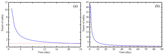
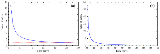
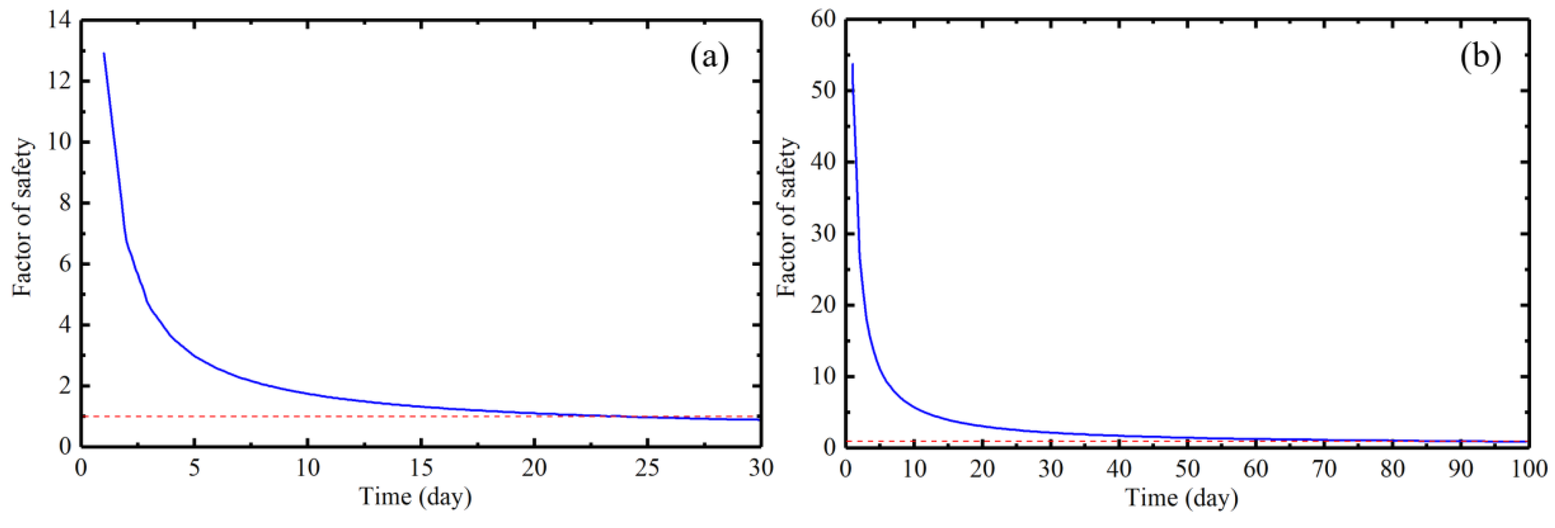
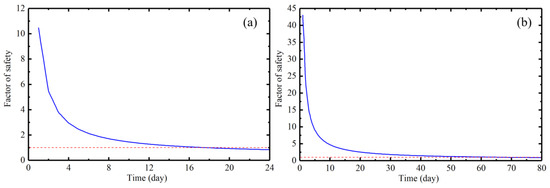
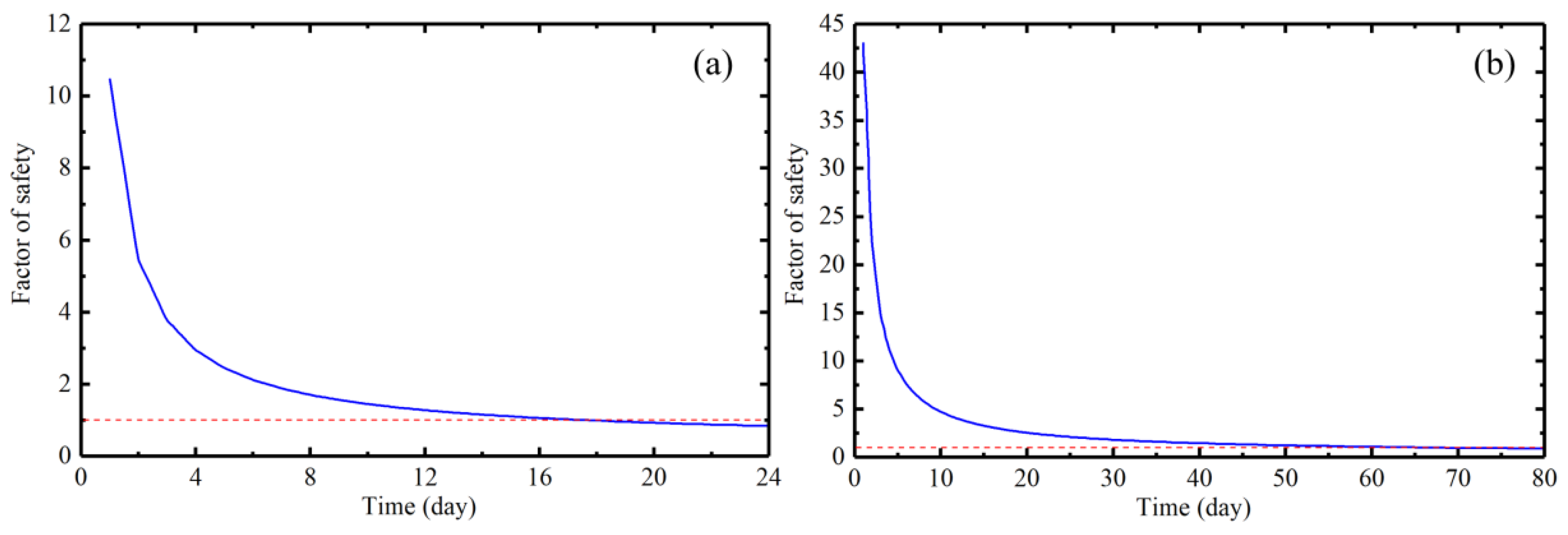
The factor of safety of the linear slope under the two rainfall conditions is shown in Figure 9. The evidence suggests that the factor of safety of the slope decreases with the continuous rainfall. During the high-intensity rainfall, the factor of safety of the slope is equal to 1.012 on the 21st d of rainfall. While under the condition of low-intensity rainfall, the factor of safety of the slope is equal to 1.005 on the 85th d. Notably, the linear slope is a meta-stable state currently. Alternatively, if the rainfall continues, the failure will occur until the factor of safety of the slope is less than 1.

Figure 9. Factor of safety of linear slope: (a) High-intensity rainfall, (b) Low-intensity rainfall.

4.2. Concave Slope Model

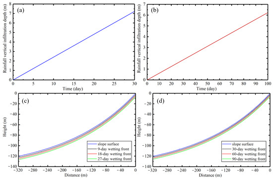
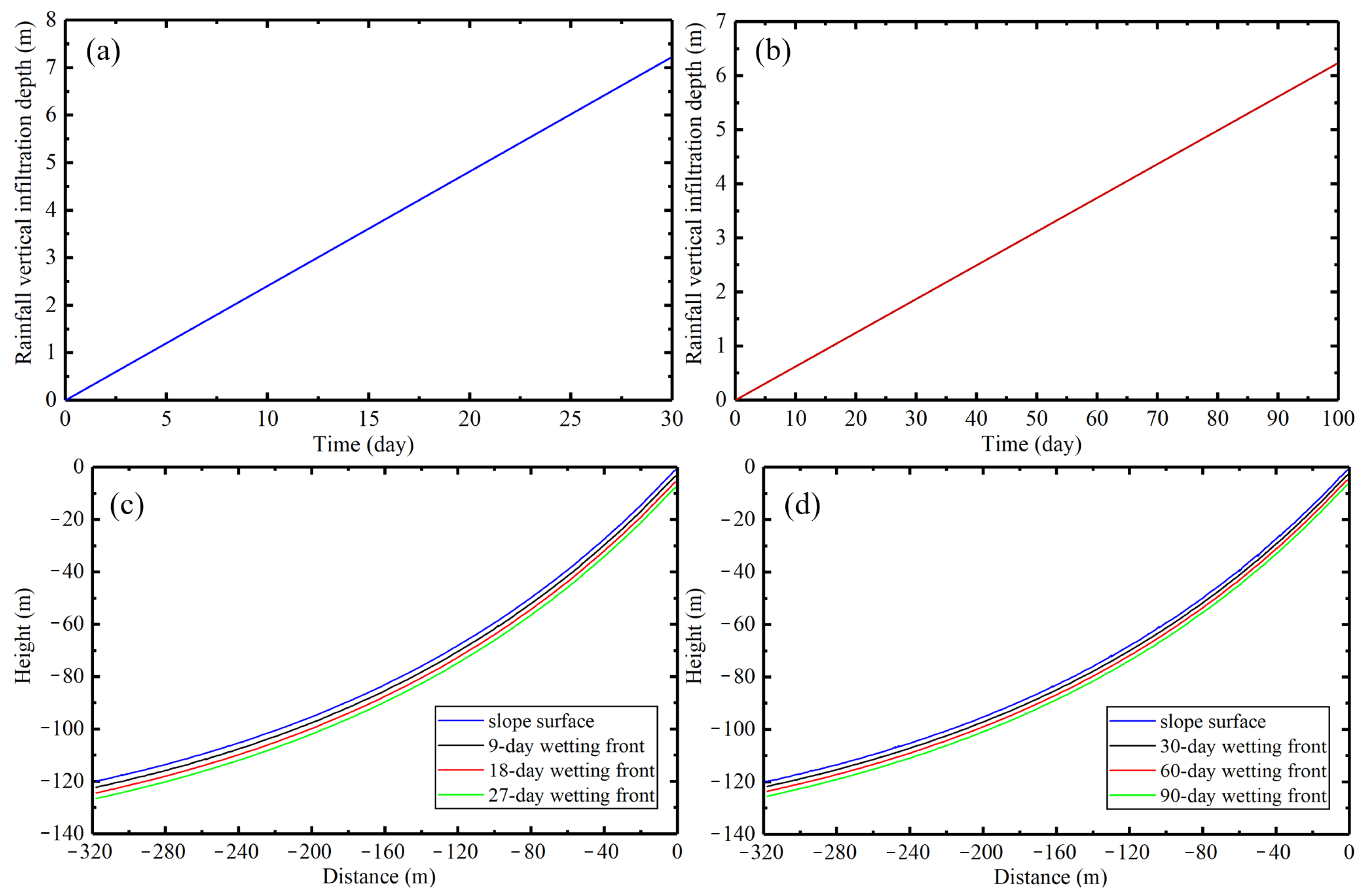
Under the condition of high-intensity rainfall (p = 85 mm/d, p > K_s), the rainfall infiltration of the concave slope is portrayed in Figure 10a. The vertical infiltration depth of the wetting front increases linearly with time. Specifically, the vertical infiltration depth of the wetting front is 5.876 m on the 24th d of continuous rainfall, which is slightly lower than the infiltration depth of the linear slope. After the continuous rainfall time reaches the 30th d, the maximum infiltration depth is 7.301 m. Then, as shown in Figure 10c, the rainfall infiltrates into the slope body continuously with the continuation of the rainfall time. During the high rainfall infiltration, the positions of the wetting front under the periods of 9 d, 18 d, and 27 d are always parallel to the slope. Additionally, under the condition of low-intensity rainfall (p = 20 mm/d, p < K_s), the rainfall infiltration situation of the concave slope is displayed in Figure 10b. Specifically, when continuous rainfall lasts for 90 d, the vertical infiltration depth of the wetting front is 5.54 m, which is less than the linear slope. Furthermore, the maximum infiltration depth is 6.25 m on the 100th d of continuous rainfall. In addition, the change trend in wetting front positions at 30 d, 60 d, and 90 d are the same as high-intensity rainfall under the condition of low rainfall intensity, which can be proven in Figure 10d.

Figure 10. Rainfall infiltration of concave slope: (a) Wetting front of high-intensity rainfall infiltration, (b) Wetting front of low-intensity rainfall infiltration, (c) Wetting front of high-intensity rainfall at various times, (d) Wetting front of low-intensity rainfall at various times.

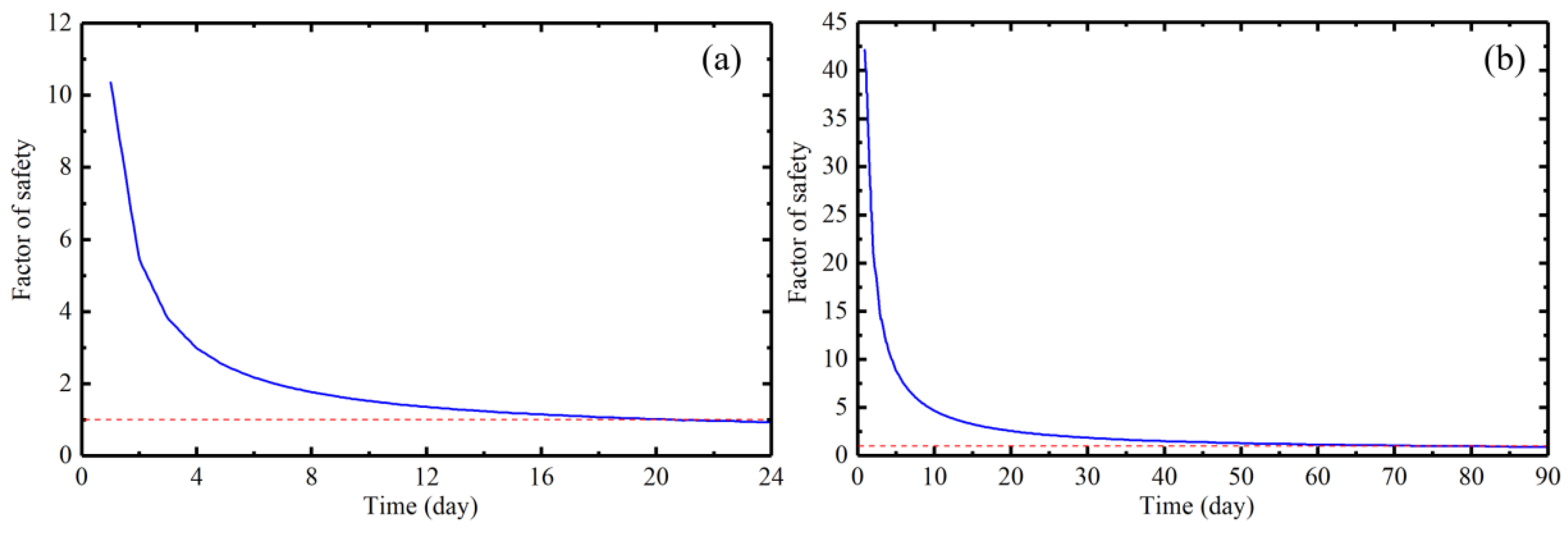
The factor of safety of the concave slope under the two types of rainfall is shown in Figure 11. It is reasonable to conclude that the factor of safety of the slope under two rainfall conditions shows an obvious downward trend with rainfall. Especially, the factor of safety of the concave slope is 1.018 after the high-intensity rainfall reaches the 24th d. Additionally, under low-intensity rainfall conditions, when the rainfall time lasts for 97 d, the factor of safety of the concave slope is equal to 1.004. Moreover, the slope is in a meta-stable state at this moment. Therefore, it can be substantiated that the failure will occur until the factor of safety of the slope is less than 1 as rainfall infiltration lasts.

Figure 11. Factor of safety of concave slope (a) High-intensity rainfall, (b) Low-intensity rainfall.

4.3. Convex Slope Model

Under the condition of high-intensity rainfall (p = 85 mm/d, p > K_s), the rainfall infiltration of the convex slope is shown in Figure 12a. It can be proven that the vertical infiltration depth of the wetting front increases linearly with time, and the vertical infiltration depth of the wetting front is 5.98 m on the 24th d of continuous rainfall, which is larger than the infiltration depth of the linear slope. Then, as shown in Figure 12c, the rainfall infiltrates into the slope body continuously with rainfall. During the high rainfall infiltration, the positions of the wetting front under the periods of 7 d, 14 d, and 21 d are always parallel to the slope. In addition, under the condition of low-intensity rainfall (p = 20 mm/d, p < K_s), the rainfall infiltration of the linear slope is shown in Figure 12b. The maximum infiltration depth is reached at 5 m when the continuous rainfall reaches the 80th d, which is also larger than that of the linear slope. Furthermore, during the low rainfall intensity, the changing trend of wetting front positions at 25 d, 50 d, and 75 d is the same as high-intensity rainfall, which can be proven in Figure 12d.

Figure 12. Rainfall infiltration of convex slope: (a) Wetting front of high-intensity rainfall infiltration, (b) Wetting front of low-intensity rainfall infiltration, (c) Wetting front of high-intensity rainfall at various times, (d) Wetting front of low-intensity rainfall at various times.

The factor of safety of the concave slope under the two types of rainfall is shown in Figure 13. The evidence suggests that the slope stability under both rainfall conditions tends to reduce with continuous rainfall. Specifically, after the high-intensity rainfall lasts for 18 d, the factor of safety of the convex slope is 1.004, while the factor of safety of the linear slope is 1.092. Additionally, under the condition of low-intensity rainfall, the factor of safety of the convex slope is equal to 1.001 on the 72nd d of continuous rainfall, which is 1.094 of the linear slopes. Therefore, it is reasonable to conclude that the linear slope appears more stable than the convex slope under the same rainfall conditions. In addition, consistent with the linear slope, if the rainfall continues infiltrating, the meta-stable state of the convex slope will be destroyed, then the factor of safety of the slope is less than 1, and failure will occur afterwards.

Figure 13. Factor of safety of convex slope (a) High-intensity rainfall; (b) Low-intensity rainfall.

4.4. Numerical Simulation Setup and Validation

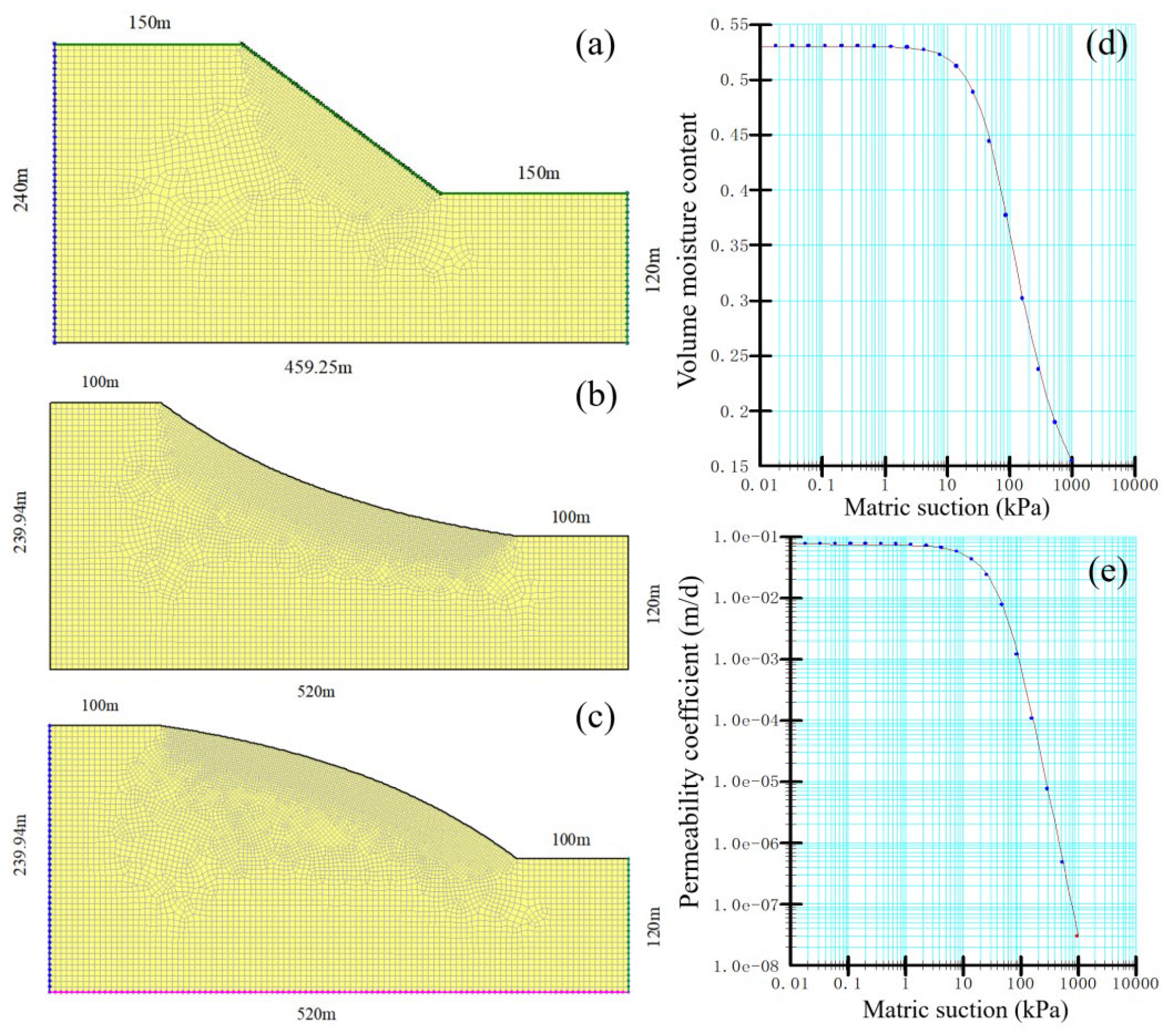
Numerical simulations were conducted using GeoStudio 2021 (SEEP/W for transient seepage and SLOPE/W for stability) to validate the analytical solutions. This software solves the Richards equation and employs the Morgenstern–Price method, making it suitable for benchmarking (Figure 14).

Figure 14. Numerical simulation model and parameters: (a) Linear slope model, (b) Concave slope model, (c) Convex slope model, (d) Volume moisture content, (e) Permeability coefficient.

Model geometry and mesh: Three slope geometries (linear, concave, convex) were discretized with mixed quadrilateral/triangular elements (max. size 0.5 m), yielding 2500–3500 elements. Halving the element size changed the factor of safety by <1%, confirming mesh independence.

Boundary conditions: The slope surface received a unit flux equal to rainfall intensity pp (m/d). The base was impervious; lateral boundaries had constant total head corresponding to the initial water table (2 m above base). Stability analysis used the entry-and-exit method (50 radius/center increments).

Hydraulic parameters: The soil-water characteristic curve and hydraulic conductivity function followed the van Genuchten model with parameters: θs = 0.45, θr = 0.05, a = 0.1 kPa⁻¹, n = 1.5, and m = 0.333 (from loess data [44,45,46]). Saturated conductivity ks = 0.075 m/d (Table 1).

Convergence criteria: Transient seepage used adaptive time-stepping with a pressure-head tolerance of 0.01 m and max. 500 iterations per step. Simulations ran up to 100 days; results were exported daily.

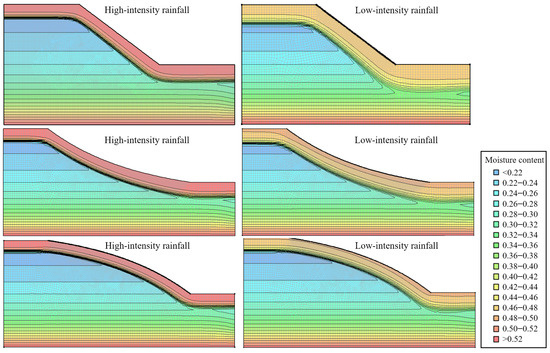
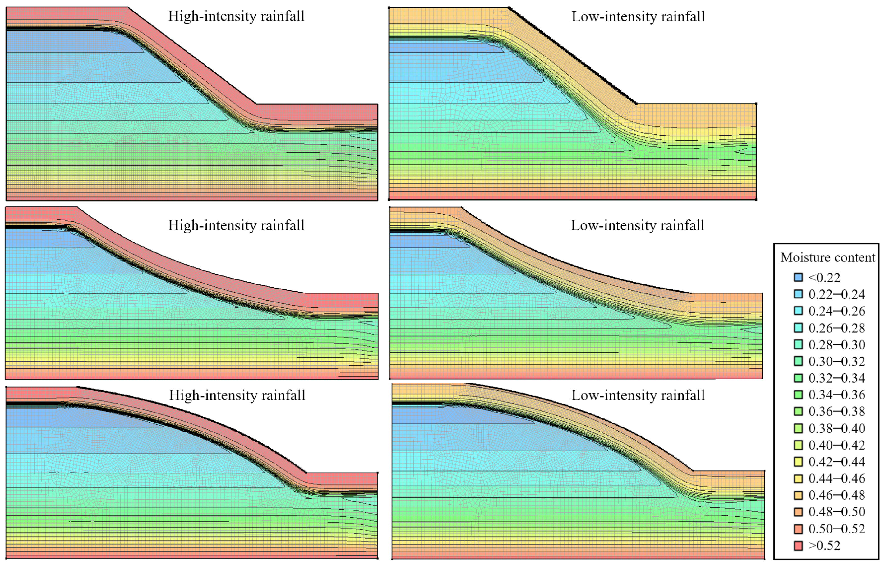
The results (Figure 15) show that the moisture content of the soil is increasing continuously due to rainfall infiltration, and the contour of the moisture content is parallel to the slope surface. In addition, based on the relationship between the wetting front and the moisture content gradient, it can be inferred that the depth of the wetting front should be parallel to the slope, which is consistent with the distribution of the wetting front obtained by the slope rainfall infiltration model. Moreover, under the same rainfall time, the infiltration depth of the wetting front at the toe slope is greater than the middle slope, which is attributed to the mutation of the fore-and-aft inclination and the change in wetting front infiltration depth. Additionally, under the action of gravitational potential energy, rainfall infiltration will also affect the flow to the head of the slope, which is consistent with the actual situation.

Figure 15. The contour map of the moisture content at the last moment of each slope model.

5. Discussion

5.1. Comparison Between Theoretical and Numerical Simulation

The factor of safety of the three slopes under the two rainfall conditions is shown in Table 2. Compared with the numerical simulation calculation results, the factor of safety of the slope and error of the theoretical model established in this paper are both within 0.05, and the failure time of the slope under the two rainfall conditions is also consistent, which can be verified in Table 2. The existence of this error is allowed under the continuous rainfall infiltration for homogeneous soil-slope. Especially, the error of factor of safety is even controlled within 0.02 for the linear slope and concave slope, which also verifies the accuracy and reliability of the model proposed in this paper.

Table 2. Comparison of stability calculation results.

Slope Shape	Rainfall	Failure Time (d)	Factor of Safety		Error
			Theoretical Calculation	Numerical Simulation
Linear slope	High-intensity rainfall	21	1.012	1.023	−0.011
		22	0.990	0.974	0.016
	Low-intensity rainfall	85	1.005	1.016	−0.011
		86	0.999	0.984	0.015
Concave slope	High-intensity rainfall	24	1.018	1.022	−0.004
		25	0.996	0.985	0.011
	Low-intensity rainfall	97	1.004	1.006	−0.002
		98	0.999	0.983	0.016
Convex slope	High-intensity rainfall	18	1.004	1.045	−0.041
		19	0.973	0.984	−0.011
	Low-intensity rainfall	72	1.001	1.017	−0.016
		73	0.993	0.984	0.009

The failure time of the linear slope, concave slope, and convex slope under rainfall infiltration shows that under the same rainfall conditions, the convex slope reaches the failure state earlier, followed by the linear slope, and finally, the concave slope. This phenomenon is related to the shape of the failure surface of the homogeneous soil-slope, which is usually arc-shaped. Due to the difference in the shape of the slope, the sliding force of the convex slope is often greater. However, the sliding force of the concave slope is the smallest. In addition, the results of rainfall infiltration also indicate that the wetting front of the convex slope is deeper, inducing the saturation area of the slid mass to increase, which will also weaken the stability of the slope.

Compared with the previous slope stability methods, we have fully considered the rainfall infiltration laws of slopes of different shapes to propose this model, which is conducive to promotion and application. However, in this paper, both the established rainfall infiltration model and the numerical simulation ignore the impact of surface water on rainfall infiltration, which is also the limitation of the current rainfall infiltration model.

To quantitatively assess the reliability of the proposed analytical models, statistical validation metrics were computed by comparing the theoretical safety factors with numerical simulation results from Table 2. The root mean square error (RMSE) is 0.018, the mean absolute error (MAE) is 0.014, and the coefficient of determination (R²) is 0.976. These low error values and high correlation coefficient demonstrate excellent agreement between the analytical predictions and numerical simulations, confirming the accuracy and reliability of the models developed in this study. The maximum relative error observed across all 12 comparison cases is less than 5%, which is within the acceptable range for engineering practice.

5.2. Influencing Factors of Slope Stability

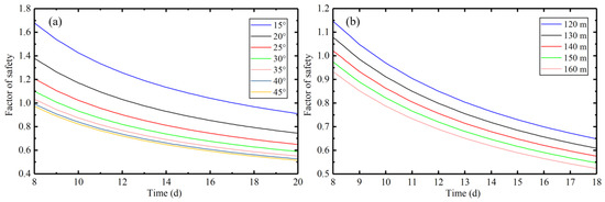
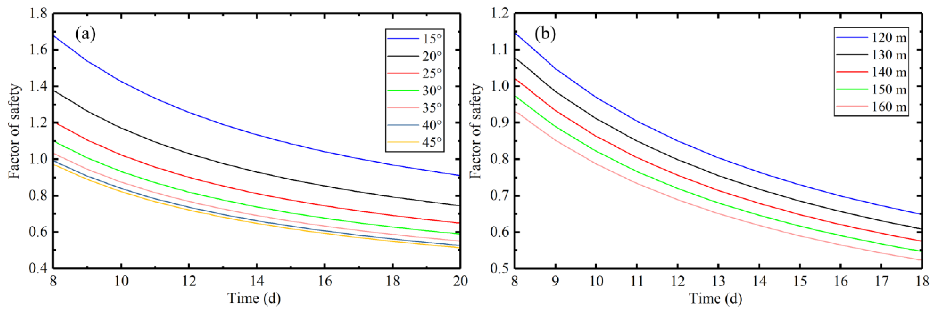
The slope stability calculation formulas for different slopes established in this paper indicate that the slope shape function of linear slope is only related to slope angle. However, the slope functions of concave and convex slopes are related to their respective maximum equivalent slope angles θ_c and the equivalent height of the slope H. Consequently, this paper takes a concave slope as an example, assuming that the rainfall intensity p = 85 mm/d, and explores the weakening law of the concave slope stability by changing the maximum equivalent slope angle θ_c and the equivalent slope height H, respectively. Figure 16a shows the relationship between the factor of safety of the concave slope and the maximum equivalent slope angle under the conditions of H = 150 m and θ_c = 15°~45° during rainfall infiltration. Additionally, under the condition of θ_c = 45°, the relationship between equivalent slope height (H = 120 m, 130 m, 140 m, 150 m, and 160 m) and the factor of safety of the concave slope is shown in Figure 16b.

Figure 16. Factor of safety of concave slope: (a) Different maximum equivalent slope angle, (b) Different equivalent slope height.

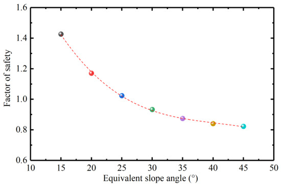
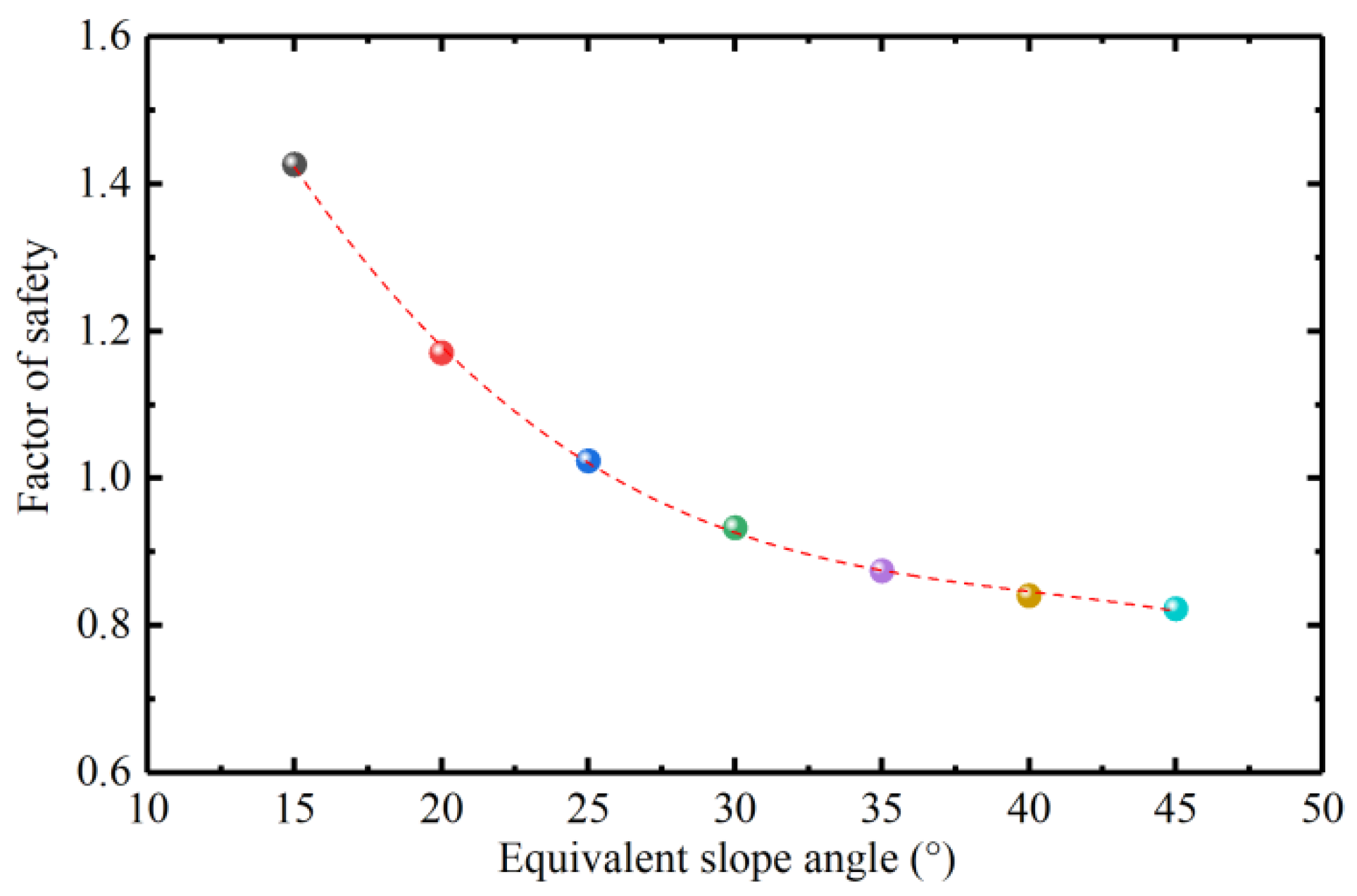
It can be substantiated in Figure 16 that the factor of safety of the slope is obviously weakened by the rainfall infiltration. Alternatively, the factor of safety of the slope is negatively related to the rainfall time and the maximum equivalent slope angle, which means the concave slope with the larger slope angle is more prone to instability failure under the action of rainfall in the interval of θ_c = 15°~45°. Moreover, under the same rainfall time, the factor of safety of the slope decreases with the increase in the equivalent slope height H. Especially, the factor of safety of the slope is the smallest when the equivalent slope height is 160 m. Therefore, it can be inferred that the concave slope with a higher equivalent slope height is more prone to failure under the action of rainfall in the interval of 120 m~160 m. Subsequently, the factor of safety of concave slopes with different equivalent slope angles on the 10th d in Figure 11a is selected for analysis. As demonstrated in Figure 17, the results indicate that there is a trend of negative correlation between the factor of safety of the slope and the equivalent slope angle. Specifically, the slope failure will occur after the equivalent slope angle reaches 26°. Moreover, the increase in the equivalent slope angle will gradually weaken the ability to decrease the factor of safety of the concave slope. In particular, when the equivalent slope angle of the concave slope is greater than 40°, the factor of safety of the concave slope will not decrease significantly.

Figure 17. Factor of safety of concave slopes with different equivalent slope angles at 10 d.

5.3. Discussion of Key Findings in Context

5.3.1. Comparison with Previous Studies and Physical Interpretation

Our results align with and extend several lines of previous research. First, the observed parallelism of the wetting front to the slope surface (Figure 8, Figure 10 and Figure 12) is consistent with Cho [11] and Damiano et al. [34]. Physically, this arises from soil isotropy and the dominance of the normal hydraulic gradient under Green-Ampt assumptions, leading to one-dimensional flow perpendicular to the slope.

Second, the stability ranking (convex < linear < concave) corroborates the 3D limit analysis of Farzaneh et al. [37] and observations of Rassam and Williams [36]. The underlying mechanism is stress redistribution due to curvature: convex slopes concentrate shear stress near the toe, while concave slopes generate a “buttressing effect” that increases confining pressure (Section 5.2). This explains why convex slopes fail 18–22% faster under our test conditions.

Third, the hyperbolic decay of factor of safety with time (Figure 9, Figure 11 and Figure 13) mirrors the infiltration-induced strength loss reported by Tsai et al. [10]. Physically, this reflects the decreasing rate of wetting front advance (Equations (24), (26) and (28)), which slows suction loss and pore pressure accumulation—consistent with landslide monitoring [7,8].

Fourth, contrasting failure times under high- and low-intensity rainfall (Section 4) arise from different pore-pressure responses. High intensity (p > K_s) rapidly builds positive pore pressure, while low intensity (p < K_s) gradually reduces matric suction. This aligns with Mein–Larson [18] and field studies [28], with our model adding explicit consideration of slope shape.

5.3.2. Engineering Applications and Practical Implications

The findings have direct implications for geohazard practice:

Early warning: Curvature-dependent thresholds—lower for convex slopes, higher for concave slopes—improve accuracy over uniform thresholds. Slope stabilization: Convex slopes require toe reinforcement (e.g., buttresses, piles) to counteract stress concentration; concave slopes benefit from the natural “buttressing effect,” often needing only localized drainage. Drainage design: Convex slopes need denser surface drainage to intercept rainfall; concave slopes benefit more from subsurface drainage at the toe. Route selection: Linear infrastructure should preferentially follow concave terrain to reduce long-term landslide risk. Hazard mapping: Coupling DEM-derived curvature with real-time rainfall enables dynamic, physics-based susceptibility mapping.

These applications demonstrate the practical value of accounting for slope shape in landslide hazard assessment.

5.4. Limitations and Implications of Model Assumptions

The analytical framework is built upon classical Green-Ampt assumptions: (1) homogeneous, isotropic soil; (2) sharp wetting front; (3) constant hydraulic conductivity behind the front; and (4) uniform rainfall infiltration. While widely adopted for tractability, these represent idealized conditions that may deviate from field realities.

In natural slopes, heterogeneity, layering, and anisotropic permeability can alter infiltration pathways. Preferential flow through macropores may produce deeper wetting fronts than predicted, accelerating failure; low-permeability layers may create perched water tables and localized pore pressures not captured by the sharp-front assumption. Such deviations could affect calculated safety factors—neglecting preferential flow may overestimate failure time (unconservative), while ignoring layering might underestimate localized instability.

The assumption of a wetting front parallel to the slope surface is critical for our treatment of curved slopes. While reasonable for shallow infiltration in homogeneous soils, it may become less accurate in highly curved slopes where lateral flow or capillary effects become significant. Future studies could refine the model by coupling with Richards equation solutions.

Despite these limitations, the framework serves as a robust mechanistic baseline. By idealizing the infiltration process, we isolate the fundamental influence of slope curvature on stability. For practical applications, model predictions should be interpreted with caution, and site-specific calibration using field measurements or more sophisticated numerical models is recommended.

6. Conclusions

In this paper, based on the establishment of the slope geological model, combined with the Green-Ampt infiltration model, the rainfall infiltration models of different slopes under high-intensity and low-intensity rainfall conditions are derived. In addition, the stability calculation models of different slopes under the two rainfall conditions are established, which is also verified by the numerical simulation method. The conclusions are as follows:

(1)

During rainfall infiltration period, the wetting front is always approximately parallel to the slope surface. Rainfall infiltration rates of different slopes are as follows: convex slope > linear slope > concave slope.

(2)

The factor of safety of the slopes keeps decreasing with rainfall infiltration. Under the condition of high-intensity rainfall, the failure time of linear, concave, and convex slopes are 21 d, 24 d, and 18 d, respectively. In addition, the failure time of the three slopes under low-intensity rainfall conditions are 85 d, 97 d, and 72 d, respectively.

(3)

Compared with the numerical simulation results, the errors of slope stability of the models proposed in this paper are all within 0.05, which also verifies the accuracy and reliability of the models proposed in this paper.

(4)

The factor of safety of the slope decreases with the increase in the slope equivalent height H and the maximum equivalent slope angle θ_c. This effect will be weakened with the increase in the equivalent slope angle. Moreover, when the equivalent slope angle of the slope is greater than 40°, the factor of safety of the concave slope will not decrease significantly.

It is important to acknowledge that while the proposed analytical models have been rigorously validated against FEM numerical simulations (a standard geotechnical benchmarking practice), direct comparison with empirical data from real-world landslides or physical experiments is lacking. This limitation stems from our primary objective: establishing a theoretical framework to isolate the fundamental effects of slope curvature under idealized, mathematically constructed geometries. Consequently, current validation confirms the models’ internal consistency and mathematical accuracy but not site-specific complexities (e.g., soil heterogeneity, vegetation, 3D topography). To address this gap, future research should apply the framework to well-documented landslide case studies, integrating high-resolution LiDAR/UAV-derived DEMs with field-monitored rainfall and pore pressure data. Such validation would assess the model’s predictive capability under complex geological conditions and inform calibrations for practical, terrain-specific hazard assessment.

References

- Juang, C.H.; Dijkstra, T.; Wasowski, J.; Meng, X. Loess geohazards research in China: Advances and challenges for mega engineering projects. Eng. Geol. 2019, 251, 1–10. [Google Scholar] [CrossRef] [Scilit]
- Tang, H.; Wasowski, J.; Juang, C. Geohazards in the three Gorges Reservoir Area, China–Lessons learned from decades of research. Eng. Geol. 2019, 261, 105267. [Google Scholar] [CrossRef] [Scilit]
- Gong, W.; Zhao, C.; Juang, C.H.; Tang, H.; Hu, X. Stratigraphic uncertainty modelling with random field approach. Comput. Geotech. 2020, 125, 103681. [Google Scholar] [CrossRef] [Scilit]
- Wu, L.Z.; Zhang, L.M.; Zhou, Y.; Li, B.E. Analysis of multi-phase coupled seepage and stability in anisotropic slopes under rainfall condition. Environ. Earth Sci. 2017, 76, 469. [Google Scholar] [CrossRef] [Scilit]
- Gong, W.; Tang, H.; Wang, H.; Wang, X.; Juang, C.H. Probabilistic analysis and design of stabilizing piles in slope considering stratigraphic uncertainty. Eng. Geol. 2019, 259, 105162. [Google Scholar] [CrossRef] [Scilit]
- Li, H.; Xu, Q.; He, Y.; Fan, X.; Li, S. Modeling and predicting reservoir landslide displacement with deep belief network and EWMA control charts: A case study in Three Gorges Reservoir. Landslides 2020, 17, 693–707. [Google Scholar] [CrossRef] [Scilit]
- Miao, F.; Wu, Y.; Xie, Y.; Li, Y. Prediction of landslide displacement with step-like behavior based on multialgorithm optimization and a support vector regression model. Landslides 2018, 15, 475–488. [Google Scholar] [CrossRef] [Scilit]
- Miao, F.; Wu, Y.; Li, L.; Tang, H.; Xiong, F. Weakening laws of slip zone soils during wetting–drying cycles based on fractal theory: A case study in the Three Gorges Reservoir (China). Acta Geotech. 2020, 15, 1909–1923. [Google Scholar] [CrossRef] [Scilit]
- Miao, F.S.; Xie, X.X.; Wu, Y.P.; Zhao, F.C. Data Mining and Deep Learning for Predicting the Displacement of "Step-like" Landslides. Sensors 2022, 22, 481. [Google Scholar] [CrossRef] [Scilit]
- Tsai, T.; Tsai, P.; Yang, P. Probabilistic modeling of rainfall-induced shallow landslide using a point-estimate method. Environ. Earth Sci. 2015, 73, 4109–4117. [Google Scholar] [CrossRef] [Scilit]
- Cho, S. Stability analysis of unsaturated soil slopes considering water-air flow caused by rainfall infiltration. Eng. Geol. 2016, 211, 184–197. [Google Scholar] [CrossRef] [Scilit]
- Gong, W.; Juang, C.H.; Wasowski, J. Geohazards and human settlements: Lessons learned from multiple relocation events in Badong, China—Engineering geologist’s perspective. Eng. Geol. 2021, 285, 106051. [Google Scholar] [CrossRef] [Scilit]
- Shi, Z.M.; Shen, D.Y.; Peng, M.; Zhang, L.L.; Wang, F.; Zhene, X. Slope stability analysis by considering rainfall infiltration in multi-layered unsaturated soils. J. Hydraul. Eng. 2016, 47, 977–985. [Google Scholar]
- Wu, Y.; Miao, F.; Li, L.; Xie, Y.; Chang, B. Time-varying reliability analysis of Huangtupo Riverside No. 2 landslide in the Three Gorges Reservoir based on water-soil coupling. Eng. Geol. 2017, 226, 267–276. [Google Scholar] [CrossRef] [Scilit]
- Miao, F.S.; Ruan, Q.Y.; Wu, Y.P.; Qian, Z.; Kong, Z.M.; Qin, Z.K. Landslide Dynamic Susceptibility Mapping Base on Machine Learning and the PS-InSAR Coupling Model. Remote Sens. 2023, 15, 5427. [Google Scholar] [CrossRef] [Scilit]
- Green, W. Studiese on soil physics-part 1, the flow of air and water through soils. J. Agric. Sci. 1911, 4, 1–24. [Google Scholar]
- Richards, L. Capillary conduction of liquids through porous mediums. Physics 1931, 1, 318–333. [Google Scholar] [CrossRef] [Scilit]
- Mein, R.; Larson, C. Modeling infiltration during a steady rain. Water Resour. Res. 1973, 9, 384–394. [Google Scholar] [CrossRef] [Scilit]
- Neuman, P. Wetting front pressure head in the infiltration model of Green and Ampt. Water Resour. Res. 1976, 12, 564–566. [Google Scholar] [CrossRef] [Scilit]
- Chu, S. Infiltration during an unsteady rain. Water Resour. Res. 1978, 14, 461–466. [Google Scholar] [CrossRef] [Scilit]
- Beven, K. Kinematic subsurface stormflow. Water Resour. Res. 1981, 17, 1419–1424. [Google Scholar] [CrossRef] [Scilit]
- Hurley, D.; Pantelis, G. Unsaturated and saturated flow through a thin porous layer on a hillslope. Water Resour. Res. 1985, 21, 821–824. [Google Scholar] [CrossRef] [Scilit]
- Habili, J.; Heidarpour, M. Application of the Green–Ampt model for infiltration into layered soils. J. Hydrol. 2015, 527, 824–832. [Google Scholar] [CrossRef] [Scilit]
- Habili, J.; Heidarpour, M.; Khalili, D. Effect of aggregate size and porosity of clay soils on the hydraulic parameters of the Green-Ampt infiltration model. J. Hydrol. Eng. 2018, 23, 06018001. [Google Scholar] [CrossRef] [Scilit]
- Stewart, R. A dynamic multidomain Green-Ampt infiltration model. Water Resour. Res. 2018, 54, 6844–6859. [Google Scholar] [CrossRef] [Scilit]
- Zhang, Q.; Chen, W.; Zhang, Y. Modification and evaluation of Green–Ampt model: Dynamic capillary pressure and broken-line wetting profile. J. Hydrol. 2019, 575, 1123–1132. [Google Scholar] [CrossRef] [Scilit]
- Alastal, K.; Ababou, R. Moving Multi-Front (MMF): A generalized Green-Ampt approach for vertical unsaturated flows. J. Hydrol. 2019, 579, 124184. [Google Scholar] [CrossRef] [Scilit]
- Huo, W.; Li, Z.; Zhang, K.; Wang, J.; Yao, C. GA-PIC: An improved Green-Ampt rainfall-runoff model with a physically based infiltration distribution curve for semi-arid basins. J. Hydrol. 2020, 586, 124900. [Google Scholar] [CrossRef] [Scilit]
- Tokunaga, T. Simplified Green-Ampt model, imbibition-based estimates of permeability, and implications for leak-off in hydraulic fracturing. Water Resour. Res. 2020, 56, e2019WR026919. [Google Scholar] [CrossRef] [Scilit]
- Qiao, J.; Wu, C.; Tian, H. Contributing ratios of the slope shape toward the landslide- development from Yunyang to Wushan in Three Gorges Reservoir Area. J. Eng. Geol. 2006, 14, 18–22. (In Chinese) [Google Scholar]
- Tang, J.; Ma, Z.; Zhou, D.; Zhang, S.; Zhang, F.; Zhou, X.; Mi, J. Numerical Modeling of Hydrological Mechanisms and Instability for Multi-Layered Slopes. Water 2024, 16, 2422. [Google Scholar] [CrossRef] [Scilit]
- Zhang, Q.; Shen, D. Rainfall-Induced Landslides: Influencing, Modelling and Hazard Assessment. Water 2024, 16, 3384. [Google Scholar] [CrossRef] [Scilit]
- Chinkulkijniwat, A.; Yubonchit, S.; Horpibulsuk, S.; Jothityangkoon, C.; Jeeptaku, C.; Arulrajah, A. Hydrological responses and stability analysis of shallow slopes with cohesionless soil subjected to continuous rainfall. Can. Geotech. J. 2016, 53, 2001–2013. [Google Scholar] [CrossRef] [Scilit]
- Capparelli, G.; Damiano, E.; Greco, R.; Olivares, L.; Spolverino, G. Physical modeling investigation of rainfall infiltration in steep layered volcanoclastic slopes. J. Hydrol. 2020, 580, 124199. [Google Scholar] [CrossRef] [Scilit]
- Sannino, G.; Bordoni, M.; Bittelli, M.; Meisina, C.; Tomei, F.; Valentino, R. Deterministic Physically Based Distributed Models for Rainfall-Induced Shallow Landslides. Geosciences 2024, 14, 255. [Google Scholar] [CrossRef] [Scilit]
- Moradi, S.; Huisman, J.A.; Vereecken, H.; Class, H. Comparing Different Coupling and Modeling Strategies in Hydromechanical Models for Slope Stability Assessment. Water 2024, 16, 312. [Google Scholar] [CrossRef] [Scilit]
- Zhou, X.; Xia, F.; Xiao, H.; Ma, Q.; Zheng, L.; Shi, Y.; Lin, Z. Response Pattern of Rainfall to the Efficiency and Threshold of Soil Water Recharge in Different Slopes. Sustainability 2025, 17, 4018. [Google Scholar] [CrossRef] [Scilit]
- Chinkulkijniwat, A.; Salee, R.; Yubonchit, S.; La Duong, H.; Horpibulsuk, S.; Hoy, M. Evaluation of cumulative rainfall and rainfall event–duration threshold based on triggering and non-triggering rainfalls: Northern Thailand case. Open Geosci. 2025, 17, 20220747. [Google Scholar] [CrossRef] [Scilit]
- Singh, K.; Bera, B. Rainfall threshold for prediction of shallow landslides in the Garhwal Himalaya, India. Nat. Hazards Res. 2024, 4, 345–358. [Google Scholar]
- Chen, G.; Zhang, K.; Li, Y.; Feng, J.; Bogaard, T. Empowering a coupled hydrological-geotechnical model to simulate long-term vegetation dynamics and their impact on catchment-scale flood and landslide hazards. J. Hydrol. 2025, 658, 133225. [Google Scholar] [CrossRef] [Scilit]
- Deng, Z.; Lan, H.; Li, L.; Sun, W. Vegetation-induced modifications in hydrological processes and the consequential dynamic effects of slope stability. Catena 2025, 251, 108793. [Google Scholar] [CrossRef] [Scilit]
- Song, F.; Duan, G.; Wang, H.; Rodriguez-Dono, A.; Wei, Y. Hydro-mechanical analysis of slope stability using anisotropic constitutive model. IOP Conf. Ser. Earth Environ. Sci. 2024, 1335, 012045. [Google Scholar] [CrossRef] [Scilit]
- Li, Z.; Yang, Z.; Teng, L.; Xie, S.; Tian, M. Machine-learning ensembled probabilistic methods for time-dependent reliability analysis of reservoir slopes under rapid water level drawdown using Bayesian model averaging (BMA). Sci. Rep. 2025, 15, 43776. [Google Scholar] [CrossRef] [Scilit]
- Gu, T.; Zhang, M.; Wang, J.; Lin, H.; Tang, Y. The effect of irrigation on slope stability in the Heifangtai Platform, Gansu Province, China. Eng. Geol. 2019, 248, 346–356. [Google Scholar] [CrossRef] [Scilit]
- Guo, Q.; Dai, F.; Zhao, Z. Analysis of the hydraulic properties of undisturbed layered loess in Northwest China. Water 2019, 11, 1379. [Google Scholar] [CrossRef] [Scilit]
- Wang, T.; Hao, Y.; Wang, Z.; Cheng, L.; Li, J. Prediction of permeability coefficient of unsaturated lime-improved loess. Chin. J. Geotech. Eng. 2020, 42, 26–31. [Google Scholar]
Disclaimer/Publisher’s Note: The statements, opinions and data contained in all publications are solely those of the individual author(s) and contributor(s) and not of MDPI and/or the editor(s). MDPI and/or the editor(s) disclaim responsibility for any injury to people or property resulting from any ideas, methods, instructions or products referred to in the content. |
© 2026 by the authors. Licensee MDPI, Basel, Switzerland. This article is an open access article distributed under the terms and conditions of the Creative Commons Attribution (CC BY) license.