


Abstract
Among the most serious types of land degradation, soil erosion poses a major threat to agricultural productivity, water quality, and ecosystem stability. Using a multidisciplinary approach, this study aimed to identify the spatial patterns of soil erosion and dominant drivers influencing soil loss in the Toplica River Basin in southern Serbia. Soil properties, including texture and organic matter content, were analyzed in samples collected throughout the study area, accounting for variations in altitude, soil type, and land use, to determine the erodibility factor (K). The rainfall erosivity factor (R), topographic factor (LS), and cover management factor (C) were determined using available inputs on rainfall erosivity, topography, land use, and vegetation cover. The Revised Universal Soil Loss Equation (RUSLE) was used to estimate annual soil erosion rates, and GIS tools and cartographic techniques were used to create spatial layers for each RUSLE factor and to generate a detailed erosion risk map. The results showed a mean annual soil loss of 5.45 t ha−1 year−1, with values ranging from 0 to 397.09 t ha−1 year−1, indicating considerable spatial variability. The regression modeling revealed the dominant roles of factors LS (β = 0.828), C (β = 0.731), and their interaction (LS × C, β = 0.561), followed by rainfall-related interactions (R × C, β = 0.268 and R × LS, β = 0.261). Two dominant erosion regimes were distinguished: topography-controlled erosion in mountainous regions and land-use-controlled erosion in low- to moderately sloping agricultural areas. The maps and analyses presented in this study provide a process-based framework for interpreting spatial erosion patterns, identifying critical hotspots and areas with higher erosion risk, and supporting more focused and context-aware conservation strategies.
1. Introduction
Sustainably managed fertile soil is essential for agriculture and for meeting future human needs, including food production, livestock feed, and access to clean water [1,2,3,4]. Given that healthy soils provide significant ecosystem services [5,6,7], close collaboration between scientists and policymakers is crucial for achieving sustainable development goals and enhancing the overall well-being of communities.
Among the causes of land degradation worldwide, soil erosion is one of the most significant, as it disrupts essential ecosystem functions, reduces biological diversity, limits agricultural output, and depletes soil organic carbon stocks. These negative impacts further contribute to broader environmental issues, including climate change, deterioration of water quality, and a decline in ecosystem resilience [8,9,10,11,12].
European soil functionality, crop production, and water quality are largely threatened by water-driven soil erosion [8]. This natural process is particularly intensified in areas where land use has been changed, leading to a loss of natural vegetation. Each year, significant amounts of fertile soil are lost to erosion, degrading millions of hectares of productive land and severely impacting agricultural productivity [13,14,15]. Erosion processes, their distribution, and timing are closely linked to anthropogenic factors, such as local social, economic, and demographic conditions [16]. Demographic factors, including population growth, density, and age structure, are key factors in shaping land use practices and, consequently, influence erosion dynamics [17,18,19,20]. Studies have demonstrated that demographic changes, including population decline and aging, lead to land abandonment and reduced agricultural activity, subsequently decreasing erosion intensity [21,22,23,24]. Conversely, intensified land use frequently elevates erosion risk in areas with stable or increasing populations. The reduction or loss of protective land cover increases soil exposure to rainfall and surface runoff, thereby enhancing its susceptibility to erosion [25].
The study of water soil erosion is supported by a wide range of methodological approaches, among which empirical methods are the most commonly applied [26,27]. Empirical models are based on statistical relationships derived from observed erosion data and are frequently used for large-scale assessments due to their simplicity and low data demand [10,28,29]. Among them, the Universal Soil Loss Equation (USLE), developed by Wischmeier and Smith (1978) [30], and its modified versions, such as the Revised Universal Soil Loss Equation (RUSLE) developed by Renard et al. (1997) [31], have been extensively applied worldwide. RUSLE accounts for environmental conditions such as relief, climate, soil properties, and human influence, incorporating factors like rainfall erosivity (R), soil erodibility (K), slope length and steepness (LS), cover-management (C), and support practices (P) to estimate the average annual soil loss resulting from interrill and rill erosion.
According to the study by Pandey et al. (2021) [32], which reviewed 160 scientific papers on soil erosion vulnerability assessment published between 1991 and 2019, RUSLE was identified as the most widely used model, applied in 42.7% of the analyzed studies, reflecting its broad acceptance and applicability across diverse geographical settings. Benavidez et al. (2018) [33] and Alewell et al. (2019) [34] also highlighted that USLE and its modifications, including RUSLE, which have a long history of use for assessing soil erosion worldwide, remain the most widely applied approaches. The popularity of RUSLE is attributed to its simplicity, adaptability, minimal data requirements, and applicability in different environments [35,36,37,38]. Advances in GIS and remote sensing have further improved the predictive capabilities of RUSLE, allowing more accurate spatial modeling of erosion potential [16].
Although RUSLE was initially developed for sheet and rill erosion on farms, it has also proven helpful for larger-scale assessments at national and continental scales [39]. Its suitability for national-scale assessments is supported by several factors: the availability of soil, topographic, climatic, and vegetation datasets, the efficient processing of large amounts of data through GIS integration, extensive scientific literature for regional comparisons, and the ability to assess both current erosion patterns and potential future climate change impacts [40].
The issue of water-induced soil erosion has been extensively addressed by the European Environment Agency (EEA) and the Joint Research Centre (JRC) of the European Commission [41], emphasizing the spatial distribution and environmental impacts of erosion across the European Union. Panagos et al. (2020) [42] estimated the mean soil erosion rate in the EU to be 2.45 t ha−1 year−1 in 2016, which is nearly identical to the 2010 value of 2.46 t ha−1 year−1, indicating a marginal decline of 0.4% over six years. A more pronounced 9% reduction was observed during the period from 2000 to 2010.
While considerable efforts have been made across much of Europe to quantify soil loss and identify erosion-prone areas, comprehensive assessments remain lacking in some regions. In recent decades, USLE and RUSLE have been applied in Serbia and neighboring countries to estimate erosion intensity and support land management planning. However, their application has typically been limited to river catchments or municipal territories, and large-scale assessments remain scarce. In Serbia, previous studies have applied the USLE and RUSLE models to specific areas, including the Bačka region, northern Serbia [43], the Kolubara District [44], and the Crveni Potok watershed in eastern Serbia [45]. Several studies by Perović and collaborators focused on eastern Serbia, including the municipality of Pirot [46], the mountainous Nišava watershed [38], and the municipality of Niš [47]. Similarly, Životić et al. (2012) [48] explored the application of USLE in southeastern Serbia, combining GIS and remote sensing. In the wider region, RUSLE has been used to assess erosion potential in the Republic of Srpska (BiH) [49] and across Romania [50].
Although previous studies have significantly advanced our understanding of soil erosion across various parts of Serbia, many regions remain unassessed by erosion modeling.
The aim of this study was to assess the spatial pattern and relative variability of erosion susceptibility in an environmentally and economically important but insufficiently studied region of southern Serbia. By integrating soil characterization, GIS-based RUSLE modeling, and erosion factor analysis, the research provides novel insights into soil erosion dynamics within the Toplica River Basin and directs soil conservation planning by identifying priority erosion hotspots. The main objectives of this research were to: (1) analyze the overall state of erosion within the Toplica River Basin to evaluate the extent and spatial distribution of erosion processes; (2) identify the most erosion-prone areas and explore the key factors driving high erosion rates; (3) determine the dominant erosion factors and assess their relative significance across different parts of the watershed; (4) investigate potential interactions among erosion factors to identify critical combinations that substantially contribute to erosion intensity; (5) evaluate the findings by comparing them with similar erosion studies conducted in Serbia and worldwide, and (6) contribute to filling gaps on the European soil erosion map.
2. Study Area
The study area encompasses the Toplica River Basin, with its western boundary defined by the eastern slopes of Kopaonik Mountain, a prominent mountain ridge in the southern Serbia (Figure 1). The basin is part of the Južna Morava River system, and the Toplica River represents its largest left-bank tributary. Kopaonik extends in a meridional direction, with its main ridge directing precipitation runoff from the eastern slopes toward the Toplica River. To the north, the basin is bordered by Veliki Jastrebac Mountain, while Radan Mountain forms the southern boundary. In contrast, the eastern side of the basin lacks a distinct morphological barrier, allowing the Toplica River to flow freely toward its confluence with the Južna Morava. Geotectonically and morphostructurally, the study area predominantly belongs to the Serbo-Macedonian Massif and, in its western part, to the Inner Dinarides, particularly to the structural framework of the Kopaonik Block. Some transitional features also indicate influence from the adjacent Vardar Zone. The Serbo-Macedonian Massif was uplifted during the Hercynian orogeny, while the Dinarides were formed during the Alpine orogeny.
Figure 1.
The Toplica River Basin and its geographical location in Serbia (red dots represent the locations of sampling points).
The relief of the Toplica River Basin includes hilly and mountainous landscapes with diverse morphological characteristics and elevation zones. The total basin area is approximately 2197 km2, with an elevation difference of over 1800 m between the highest point in the west, on Kopaonik Mountain (2017 m), and the lowest point near its confluence with the Južna Morava River (approximately 187 m above sea level). The average elevation of the basin is 632 m above sea level, with lacustrine sedimentation and fluvial erosion and sedimentation during the Quaternary period.
The geological structure of the Toplica River Basin is complex, resulting from the interplay of rock formations of different ages, lacustrine phases, fluvial processes, and tectonic activity. In the western part of the basin, on the slopes of Kopaonik Mountain, the geological structure includes various types of igneous rocks of different ages, ranging from the Paleozoic to the Miocene and Pliocene, as well as sandstones, conglomerates, breccias, siltstones, and marlstones of Cretaceous age. Endogenous tectonic processes during the Tertiary shaped the primary morphostructural forms of Kopaonik Mountain, which were later modified by exogenous forces during regression and uplift. Moving eastward, the mountainous terrain is predominantly composed of ancient Paleozoic metamorphic rocks, but includes igneous formations of varying ages, primarily from the Oligocene and Miocene. In the northern part of the basin, on Jastrebac Mountain, the terrain consists of different schists and metamorphosed gabbros, with sporadic occurrences of igneous rocks, particularly gneiss-granites. The southern part of the basin is characterized by widespread occurrences of andesites and pyroclastic rocks, along with clastic rocks composed of volcanic material (tuff, tuffaceous gravel, breccia). The lower parts of the basin, particularly north of the Toplica River, are composed of Miocene lacustrine sediments consisting of gravel, siltstones, clays, and claystones. In this section of the basin, the area along the river is built upon alluvium, above which river terraces rise. Towards Jastrebac Mountain, lacustrine sediments transition into unsorted proluvial and deluvial deposits, transported by mountain streams [51,52]. Due to the basin’s lithological and hydrogeological characteristics, water retention above the erosion base is minimal, resulting in rapid surface runoff during periods of increased precipitation and reduced flow during dry periods [51].
The complex geological structure, intricate climatic characteristics, and associated natural vegetation significantly influence the high diversity of soil types within the Toplica River Basin. In the mountainous areas, where the geological substrate consists of metamorphic and igneous rocks, Vertic Cambisols (Eutric) and Vertic Cambisols (Dystric) are most commonly found, along with Haplic Cambisols (Eutric), Umbric Leptosols (Dystric), and Podzols. Vertic Cambisols (Eutric) are predominantly developed on lacustrine sediments, although smaller areas also exhibit Haplic Cambisols (Eutric). Along rivers, in fluvial deposits, the most prevalent soils are Haplic Fluvisols (Eutric), with less frequent Haplic Fluvisols (Calcaric) [52].
From a biogeographical perspective, Kopaonik Mountain exemplifies the altitudinal vegetation stratification within the northern temperate climatic zone. Vegetation composition is influenced by edaphic factors, regional climatic circulation, and the meridional orientation of the mountain massif. Approximately 1600 plant species have been recorded on Kopaonik, of which 825 belong to the high-mountain flora [53]. These factors cause local differences in vegetation composition between the northern and southern slopes, as well as between the eastern and western sides, separated by the main mountain ridge. The lowest vegetation zone consists of mixed deciduous forests dominated by oak species (Quercus). Thermophilous oak forests occupy the submontane and lower montane belts up to approximately 800 m a.s.l. Above this zone, forests of Sessile oak (Quercus petraea) and Turkey oak (Quercus cerris). In the northern part of Kopaonik Mountain, stands of Balkan beech (Fagetum moesiacae submontanum) are present [54].
Historically, Kopaonik was known for extensive spruce (Picea) forests on podzolic soils. Today, these forests are largely preserved only in fragmented patches within Kopaonik National Park [53], while illegal logging and insufficient regeneration in unprotected areas continue to disrupt the natural cycle. The consequences of deforestation and forest degradation are significant for soil stability, as the removal of vegetation and root systems leaves relatively young soils exposed and prone to erosion. Some stands have also been affected by drought-induced tree mortality, caused by regional climate changes and uneven summer precipitation.
The Toplica River Basin lies within the moderate continental climate zone. Precipitation is the most important climatic factor influencing erosion processes. This basin is among the driest regions in Serbia. At the meteorological station in Kuršumlija, located in the basin’s central part, average annual precipitation is approximately 650 mm. At higher elevations, precipitation increases, exceeding 900 mm at the highest peaks of Kopaonik Mountain. Precipitation is relatively evenly distributed throughout the year, with a maximum from May to July (60–66 mm per month) and a minimum in August (42 mm), January (42 mm), and February (45 mm). A substantial snowpack accumulates in the mountainous areas during winter and melts in spring. Snow cover persists for a particularly long time on Kopaonik, averaging over five months per year. This snowmelt often coincides with peak rainfall, significantly increasing runoff volumes and surface water erosion [55].
3. Materials and Methodology
3.1. Sampling Approach
Soil samples were collected at 46 locations (Figure 1; Table A1) distributed throughout the basin. The sampling points were not laid out on a regular grid; rather, a stratified random sampling design was used to ensure all major sub-regions and land uses within the basin were represented. This allowed us to capture the spatial variability of soil properties across the study area. The sampling included sites under forest (18 sites; 39%), grassland (22 sites; 48%), and agricultural land use (6 sites; 13%), to ensure representativeness across the basin’s main land cover categories. In terms of lithology, the sampling points were distributed across consolidated sedimentary rocks (23 sites; 50.0%), magmatic rocks (10 sites; 21.7%), metamorphic rocks (8 sites; 17.4%), and unconsolidated Quaternary sediments (5 sites; 10.9%), thereby covering the principal geological units that influence soil formation and erosion processes. One composite soil sample was collected at each location from the 0–30 cm depth interval with an auger (Eijkelkamp, Giesbeek, The Netherlands). The disturbed soil samples were immediately placed in labeled plastic bags and sealed to prevent moisture loss or loss of fine soil particles during transport. To determine soil dry bulk density (BD), undisturbed samples were collected using standard steel core rings (5 cm height × 5 cm diameter, 100 cm3). The cylinders were carefully extracted from the soil to prevent soil loss or changes in the sample structure. Sampling points were positioned using a GPS device (TDC100 GPS, Trimble GmbH, Raunheim, Germany).
3.2. Soil Analysis
Soil samples collected from the study area were analyzed for key properties influencing water erosion, including dry bulk density (BD), particle size distribution and coarse fraction content, total organic carbon (TOC), soil structure class (S), and soil permeability (P), with detailed values for each sampling location provided in Table A1. Prior to texture analysis, the soil was sieved at 2 mm to remove the coarse fraction (particles > 2 mm diameter). The remaining fine-earth fraction (<2 mm) was then used for particle size distribution determination.
3.2.1. Dry Bulk Density (BD)
The soil’s dry bulk density (BD) was determined using the Kopecky core method in accordance with the international standard [56]. The samples were dried at 105 °C to a constant weight.
3.2.2. Determination of Particle Size Distribution and Skeletal Content
The determination of the granulometric composition and skeletal content of the soil was conducted according to the standard [57]. The soil samples were first dried to a constant weight to remove moisture and then sieved through a 2 mm mesh to separate the skeletal material from the fine fraction. The skeletal content was expressed as a percentage by mass relative to the sample’s total mass. Organic matter was removed by adding hydrogen peroxide and heating, while carbonates were eliminated by adding a hydrochloric acid solution. Sand fractions, including fine sand (0.05–0.1 mm) and medium to coarse sand (0.1–2.0 mm), were determined by sieving through a series of appropriately sized sieves, while silt (0.002–0.05 mm) and clay (<0.002 mm) fractions were separated by sedimentation.
3.2.3. Total Organic Carbon (TOC)
The organic carbon content was determined in accordance with ISO 14235:1998 [58], a widely used standard in soil research due to its accuracy and simplicity. The water content in the samples, expressed as a percentage of dry mass, was determined according to ISO 11465:1993 [59]. A Lambda 40 spectrophotometer (Perkin Elmer, MA, USA) was used for the spectrophotometric determination of organic carbon. To ensure the accuracy and precision of the results, control samples with known organic carbon content were analyzed, along with blank samples, to eliminate contamination-related measurement errors. Each measurement was performed in triplicate on the same soil sample, and the three results were averaged.
3.2.4. Soil Structure Class (s)
The soil structure class was determined using data from the European Soil Data Centre [60]. The classification was based on pedological parameters, including soil type according to the Food and Agriculture Organization (FAO) classification [61] and soil texture. Based on these characteristics, soil structures were categorized as humic, poor, normal, or good (Table 1).
Table 1.
Soil structure classes according to the ESDAC classification.
3.2.5. Soil Permeability (p)
Soil permeability classes were assigned based on the soil texture classes described in USDA, 1983 [62] (Table 2).
Table 2.
Soil permeability classes based on soil texture.
3.3. Development of the RUSLE Model Factors for Soil Erosion Estimation
The RUSLE is an empirical model used to estimate soil erosion. The equation (Equation (1)) calculates the average annual soil loss (A) as follows:
where A is average annual soil loss rate (t ha−1 year−1); R is rainfall erosivity factor (MJ mm ha−1 h−1 year−1); K is soil erodibility factor (t ha h ha−1 MJ−1 mm−1); LS is topographic factor (dimensionless); C is a cover management factor (dimensionless); and P is a support practice factor (dimensionless).
3.3.1. Rainfall Erosivity Factor (R)
The R factor in the USLE and RUSLE models represents rainfall erosivity. In the original USLE framework, rainfall erosivity is defined based on storm kinetic energy and maximum 30-min rainfall intensity (EI30) derived from standard plot conditions, where other RUSLE factors are assumed constant. This factor measures the impact of rainfall on soil erosion, a relationship initially observed through sediment deposits after intense storms [30]. The R factor reflects the erosive force of rainfall, quantifying the kinetic energy of raindrops and the potential for resulting runoff in terms of volume and rate [31,63]. Calculating the R factor can be challenging because comprehensive rainfall data may not be available in all regions. Accurate localized precipitation data are essential for precisely computing the R factor, underscoring the link between rainfall characteristics and soil erosion potential. The study uses the MeteoSerbia1km dataset, the first daily gridded meteorological dataset at a 1 km spatial resolution across Serbia for the 2000–2019 period [64].
The empirical equation (Equation (2)), originally developed by Arnoldus (1977) [65] for estimating rainfall erosivity, and later corrected to properly incorporate the conversion factor [66] (Chen et al., 2023), was used due to the lack of high-temporal-resolution rainfall intensity data for the study area as follows:
where R—rainfall erosivity factor in MJ mm ha−1 h−1 year−1, Pi—monthly precipitation in mm, and P—annual precipitation in mm.
The ArcMap 10.4.1 Model Builder was employed to automate the processing of raster-based precipitation data. The process started with data normalization, as all original datasets are stored as integers (INT32 data type) to reduce the size of the GeoTIFF files. Precipitation rasters are divided by 10 to obtain precipitation data in millimeters.
After normalizing the data, the annual R factor was computed using the Raster Calculator tool. To obtain a long-term perspective on rainfall erosivity, the annual R factors were averaged over the 18-year study period using the Cell Statistics tool (data from the 2000 were excluded due to missing monthly datasets in the Zenodo repository).
3.3.2. Soil Erodibility Factor (K)
The Soil Erodibility Factor (K) quantifies the resistance of soil or surface materials to erosion by evaluating their susceptibility to detachment and transport by rainfall and runoff. K factor assesses the soil’s ability to withstand the impact of raindrops and the consequent rate and volume of runoff under standardized conditions [67]. The K factor is derived using Equation (3) [30,31]:
where K—soil erodibility factor (t ha h ha−1 MJ−1 mm−1), M—particle size parameter, calculated as (% silt + % very fine sand) × (100 − % clay), OM—organic matter (%), calculated by multiplying TOC by the Van Bemmelen factor (1.724), s—soil structure code, p—soil permeability class, 0.1317—factor for conversion to SI units. Due to the limited number and spatial distribution of soil samples (n = 46), the K factor was interpolated using the Inverse Distance Weighting (IDW) method and interpreted as a generalized spatial representation.
3.3.3. Slope Length and Slope Steepness Factor (LS)
The topographic factor (LS) is the soil loss ratio at a specific site compared to a baseline site, with a standard slope steepness of 9% and a slope length of 22.13 m [68]. LS factor includes two primary components: the slope length factor (L) and the slope steepness factor (S) [69]. Each component contributes to the rate of soil erosion on a given landscape. As the slope length increases, more runoff accumulates and flows downhill, increasing soil erosion. Similarly, increased slope steepness causes runoff to move faster, enhancing its ability to erode soil [63,70].
To calculate the LS factor, data from the Shuttle Radar Topography Mission (SRTM) [71], a digital elevation model (DEM) with a 30 m × 30 m resolution, were used. This is the highest-resolution topographic dataset currently available for Serbia. A detailed assessment of the topographic conditions contributing to soil erosion was provided using these high-resolution data. The DEM was preprocessed by applying a fill-sinks algorithm developed by Wang and Liu (2006) [72], which effectively identifies and removes surface depressions in the elevation data. The methodology for calculating the LS factor was based on the approach proposed by Moore et al. (1991) [73], which integrates both slope length and slope steepness.
3.3.4. Cover Management Factor (C)
The cover management factor (C) reflects how different land cover types affect soil protection against erosion. Vegetation cover acts as a barrier shielding the soil surface from the direct impact of raindrops and dissipating their energy of the raindrops [74] before they reach the soil. Vegetative characteristics influence the soil’s ability to absorb water, slow down runoff, and thus reduce the potential for erosion. The value of the C factor is directly influenced by vegetation type, growth stage, and the percentage of the ground covered by vegetation [67].
The C factor values are assigned to all land use types based on the values cited in the literature [44,75]. The ESA WorldCover dataset, based on Sentinel-1 and Sentinel-2 data, was used as the land cover input [76]. The ESA WorldCover data, initially at 10 m × 10 m resolution, was resampled to 30 m × 30 m using nearest-neighbor interpolation to align with other datasets and ensure consistency in the analysis. The C factor values assigned to specific land cover types ranged from 0 for built-up areas, permanent water bodies, and herbaceous wetlands, where soil erosion is effectively absent due to sealed or non-erodible surfaces, to 0.004 for tree cover, 0.05 for shrubland, 0.1 for grassland, 0.15 for cropland, and 0.3 for bare or sparsely vegetated areas.
3.3.5. Support Practice Factor (P)
The support practice factor (P) value is the ratio of the amount of soil loss after soil conservation measures to the amount of soil loss without any soil conservation measures [77,78]. Field observations revealed that no specific soil conservation practices, such as contour farming, strip cropping, terracing, grassed waterways, windbreaks or conservation tillage, are currently in place in the study area. Therefore, the P factor has been set to 1.0 throughout the entire region, meaning that no interventions to reduce soil loss from erosion are considered in the erosion estimates, and the current erosion susceptibility of the terrain is fully represented. Similar assumptions have been made in previous studies, where the P factor was also set to 1.0 in the absence of soil conservation practices [79,80,81,82,83,84].
3.4. Statistical Analysis
Statistical analysis was performed for each input factor of the RUSLE model and for the resulting erosion rates, including minimum, maximum, range, mean, standard deviation, coefficient of variation, and percentiles (5th, 25th, 50th [median], 75th, and 95th). For that purpose, raster layers generated in the GIS environment were used, including those for rainfall erosivity (R), soil erodibility (K), slope length and steepness (LS), cover management (C), and erosion rates (t ha−1 year−1). Data processing in QGIS 3.40.4 [85] included raster preparation, reprojection, resampling, map algebra, and spatial overlay operations. The K factor was derived from soil property data obtained at 46 sampling locations and interpolated to a continuous raster, while the LS factor was calculated from a DEM, and the C factor was assigned based on land cover data. Statistical analysis of raster layers was performed in SAGA GIS 9.7.1 using the Spatial and Geostatistics—Statistics for Grid module [86].
Additionally, the relationships between the calculated RUSLE erosion rates and the individual RUSLE factors, as well as selected soil properties, were examined through Spearman correlation analysis (ρ). This non-parametric approach was chosen because the data deviated from normality, as indicated by the Shapiro–Wilk test [87]. Correlation coefficients and corresponding p-values were calculated to assess the strength and statistical significance of the relationships. Regression analysis was additionally performed to analyze the contribution of interactions between the RUSLE factors. Calculations were conducted using Excel software [88].
4. Results and Discussion
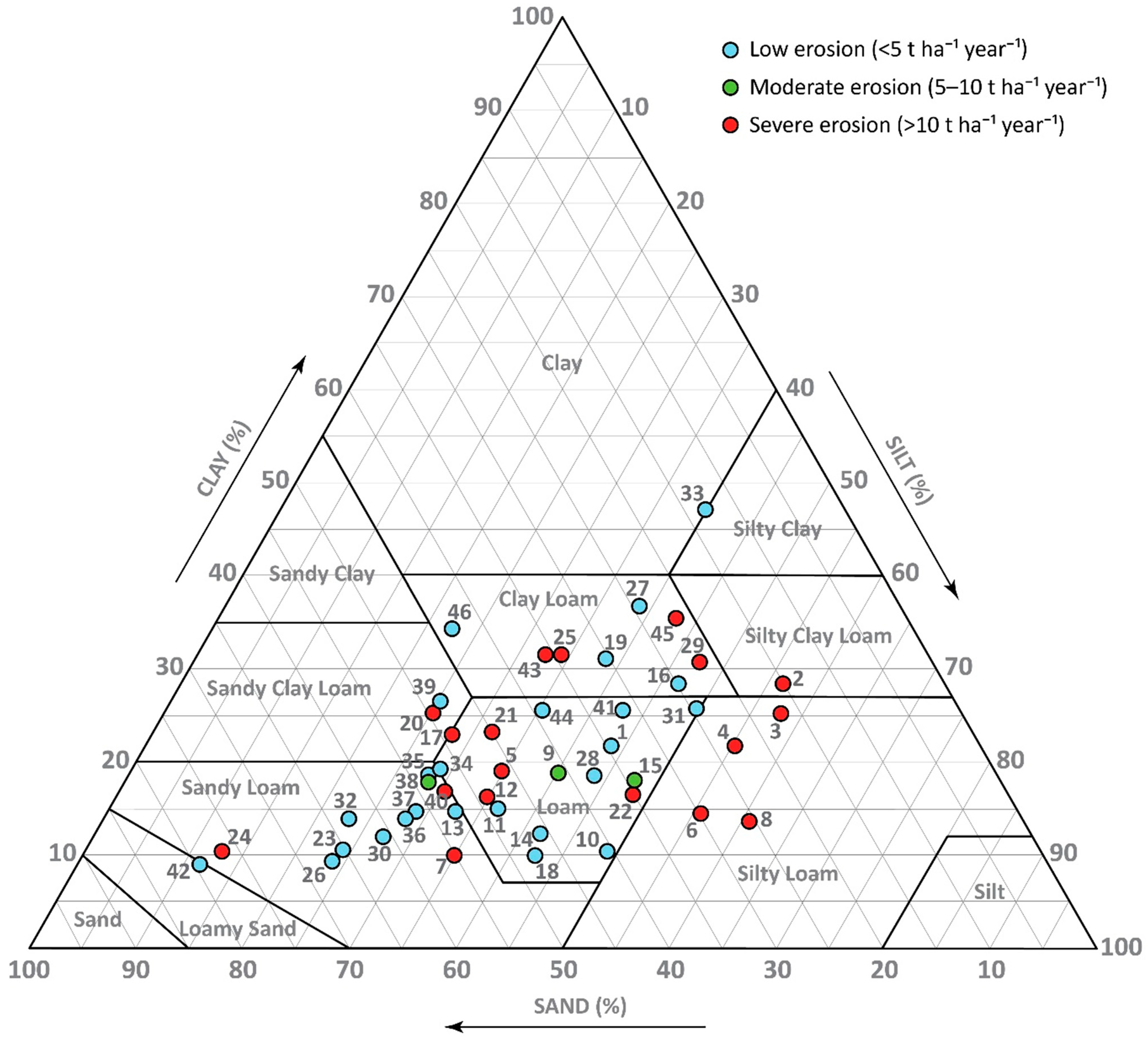
The results of this study are presented in terms of the RUSLE factors—rainfall erosivity (R), soil erodibility (K), slope length and steepness (LS), and cover management (C)—as well as the calculated soil erosion rates, with detailed values for each sampling location provided in Table A1. In addition, the USDA textural classification of the soil samples, colored according to EU erosion severity classes, is shown in Figure A1.
4.1. Analysis of Rainfall Erosivity (R) Factor
The rainfall erosivity factor in the study area ranges from 1194.9 to 3117.7 MJ mm ha−1 h−1 year−1, with a mean value of 1586.3 (Table 3). The dataset shows a noticeable range of values (1922.8 MJ mm ha−1 h−1 year−1) and a standard deviation of 341.8, suggesting some variability in rainfall patterns and their erosive potential across the catchment. However, the coefficient of variation (CV = 22%) indicates that this variability is moderate rather than high, implying a relatively consistent R factor values within the catchment. The R factor distribution shows a clear gradient, with higher values observed in the mountainous regions (Figure 2), particularly in the western part of the basin, where the highest values are recorded on Kopaonik, the highest mountain in the study area. This trend aligns with the overall decrease in annual precipitation from west to east across Serbia [89,90]. Elevated precipitation values are also observed in the northern and southern mountainous areas, such as Jastrebac and Radan, consistent with previous studies [91,92]. In contrast, the lowest R factor values are found in the lower-lying areas, particularly in the valleys of the Toplica River and its main tributaries, as well as in the eastern parts of the basin. The distribution of R factors likely reflects climatic variations in precipitation and topographical influences on rainfall patterns.
Table 3.
Descriptive statistics of RUSLE erosion factors and RUSLE erosion rates in the study area.
Figure 2.
The R factor map of the study area for the period 2001–2019 (MJ mm ha−1 h−1 year−1).
Both the mean value and the percentile distribution (Table 3) indicate that lower R factor values predominate. The fact that the 5th percentile (1274.1 MJ mm ha−1 h−1 year−1) is relatively close to the mean (1586.3 MJ mm ha−1 h−1 year−1), while the 95th percentile (2359.9 MJ mm ha−1 h−1 year−1) is much higher, indicates a right-skewed distribution. Most areas within the basin experience moderate to low rainfall erosivity, while a few locations are subjected to intense erosive rainfall events.
For comparison, previous studies conducted in similar areas in the broader region (Bosnia and Herzegovina) have reported R factor values ranging from 2778.82 to 3656.34 MJ mm ha−1 h−1 year−1 in the Pale Municipality [93], from 1288.01 to 1431.02 MJ mm ha−1 h−1 year−1 in the northern part of the country [94], and from 826.7 to 4934.5 MJ mm ha−1 h−1 year−1 in the Republic of Srpska [49]. Additionally, a study conducted in Northwestern Crete, Greece, which shares comparable Mediterranean climatic influences, reported R factor values ranging from 348 to 3687 MJ mm ha−1 h−1 year−1 [95].
4.2. Spatial Distribution of Soil Erodibility (K) Factor
In the study area, the soil erodibility factor ranges from 0.0155 to 0.0676 t ha h ha−1 MJ−1 mm−1, with a total span of 0.0521 t ha h ha−1 MJ−1 mm−1 (Table 3). The mean value is 0.0436 t ha h ha−1 MJ−1 mm−1, and a standard deviation of 0.0073 t ha h ha−1 MJ−1 mm−1, along with a coefficient of variation of 17%, indicates that most soils have relatively similar erodibility properties. Moreover, the differences between the values of the 5th and 25th, 25th and 50th, 50th and 75th, and 75th and 95th percentiles (Table 3) are similar, indicating a uniform distribution of the K factor across the river basin, with few extreme outliers and no significant skew toward unusually high or low values. The spatial distribution of the soil erodibility factor (Figure 3) does not exhibit a clear pattern. Both high and low values are found across a range of elevations, from higher mountainous regions to lower-lying areas, and occur in a variety of soil types, geological formations, and vegetation cover types. The lack of a clear spatial trend suggests that soil erodibility in the study area is influenced by an interplay of multiple factors, including soil texture, organic content, and local topography, rather than being primarily dictated by any single environmental variable.
Figure 3.
The K factor map of the study area (t ha h ha−1 MJ−1 mm−1).
In line with this interplay of multiple controlling factors, the distribution of the K factor, which characterizes soil susceptibility to erosion, shows no clear spatial pattern and is influenced by individual sampling points. While this provides a general overview of areas with relatively higher or lower soil erodibility, local values may be over- or underestimated, particularly in sparsely sampled areas. Consequently, the K-factor map should be used to identify broad spatial tendencies rather than precise site-specific predictions.
Previous studies in geographically and climatically comparable regions have reported the soil erodibility factor (K) in the range of 0.01 to 0.08 t ha h ha−1 MJ−1 mm−1 in Romania [50], 0 to 0.07 t ha h ha−1 MJ−1 mm−1 in Southeastern Serbia [48] and Pirot Municipality, Serbia [46], and 0 to 0.061 t ha h ha−1 MJ−1 mm−1 in the Republic of Srpska (Bosnia and Herzegovina, BiH) [49]. These studies, conducted in areas with similar topographic and climatic conditions, show soil erodibility orders of magnitude similar to those observed in our study area, further supporting the consistency of soil erodibility characteristics across the region.
4.3. Analysis of Slope Length and Steepness (LS) Factor
The LS erosion factor ranges from 0 to 73.153, with an average of 4.123 and a standard deviation of 3.334 (Table 3; Figure 4). The highest LS values are found in the mountainous areas, particularly in the western part of the basin in Kopaonik, where the terrain is steep and dissected. Additionally, higher LS values are observed in the mountains to the north and south of the river basin, where steep slopes are common. It should be emphasized that the 30 m DEM resolution may smooth local slope extremes and underestimate absolute LS magnitudes in these steepest parts of the study area. On the other hand, lower LS values are recorded in the river valleys, particularly along the main river, Toplica, and in the flatter terrain north of the Toplica River and the downstream, eastern part of the river basin. These areas, with gentler slopes and lower LS values, reflect the reduced potential for erosion.
Figure 4.
The LS factor map of the study area.
The differences between the 25th and 50th percentile values, as well as between the 50th and 75th percentile values, are nearly identical, indicating a relatively consistent distribution of LS values within these ranges (Table 3). However, the difference between the 5th and 25th percentile values is considerably smaller than between the 75th and 95th percentile values. This pattern suggests that higher LS values are less frequent. Additionally, the difference between the minimum value (0) and the 5th percentile is much smaller than that between the 95th percentile and the maximum value (73.153), further supporting the idea that extreme values are rare.
In the Pirot Municipality, Serbia, values of the LS factor reflected a similar distribution, with steep, dissected mountainous areas showing higher values [46]. Similarly, in the Lower Kulsi Basin, India, the LS factor ranged from 0 to 80.5 [96], showing a pattern of higher values in steeper terrain and lower values in flatter areas, which aligns with the findings of our study.
4.4. Cover Management (C) Factor Analysis
The distribution of land cover types within the basin, derived from ESA data (Table 4), plays a crucial role in determining the cover management factor (C) and its influence on erosion potential. Forested areas (tree cover) dominate the landscape, covering 67% of the basin, predominantly in the mountainous and hilly regions in the north, west, and south.
Table 4.
Land cover types and their respective areas based on ESA data.
Forested areas are interspersed with grassland, forming a mosaic-like pattern, except on Jastrebac Mountain, where continuous forested expanses prevail. Due to dense vegetation and well-developed root systems, tree-covered areas contribute to lower C values, offering significant protection against soil erosion by reducing raindrop impact, surface runoff, and soil detachment (Figure 5). Grassland, occupying 21% of the basin provides moderate erosion protection. Compared with forest cover, grassland exhibits slightly higher C values due to its lower canopy cover and weaker root structures, which allow increased surface runoff and soil displacement in steeper regions. Cropland, covering 10% of the basin, is predominantly located in the lower reaches of the Toplica River, in the eastern part of the basin, and in the valley between the Toplica River and the slopes of Jastrebac Mountain. These areas, particularly when cultivated with annual crops and subjected to tillage, exhibit the highest C values, making them more vulnerable to soil erosion. The lack of permanent vegetation cover increases exposure to rainfall impact and surface runoff, leading to increased soil loss.
Figure 5.
The C factor map of the study area.
Although occupying a smaller portion of the basin, built-up areas (1.094%) and bare or sparsely vegetated surfaces (0.021%) also contribute to variations in erosion susceptibility. While built-up surfaces are largely impervious, preventing soil erosion directly, bare areas exhibit some of the highest C values due to minimal vegetation cover and increased susceptibility to surface runoff. Other minor land cover classes, including shrubland (0.003%), permanent water bodies (0.012%), and herbaceous wetlands (0.004%), have negligible effects on overall erosion processes. However, despite their small coverage, wetlands can act as sediment retention zones, helping reduce sediment transport in localized areas.
The types of land cover across the basin strongly influence the C factor. Forested areas tend to have the lowest erosion potential, while cropland and bare soil contribute more to erosion risks. This pattern clearly shows the importance of land cover in mitigating erosion, highlighting the need for sustainable land use and cover to minimize soil loss.
The descriptive statistics (Table 3) support this pattern, as over half of the basin has very low C values (≤0.0041), which are mostly associated with forest and grassland. However, higher C values appear in the upper percentiles, for example, 0.1006 at the 75th percentile and 0.1500 at the 95th percentile, reflecting cropland and sparsely vegetated areas. While the maximum C value (0.3) indicates a potential for high erosion risk, such extreme values are rare, reinforcing that most of the basin is covered by areas less prone to erosion, such as forests and grasslands.
4.5. Soil Erosion Rates from RUSLE
The results of the RUSLE model exhibit substantial spatial heterogeneity across the study area, which can be attributed to the combined influence of multiple erosion factors with varying magnitudes and spatial distributions. Despite this complexity, several general patterns of estimated soil erosion intensity can be identified. Although some parts of the basin exhibit high erosion rates, most of the watershed falls onto the low-erosion category, with soil loss values below 5 t ha−1 year−1. As shown in Table 5, low erosion areas (<5 t ha−1 year−1) cover approximately 78% of the watershed, with the most considerable portion falling within the 2–5 t ha−1 year−1 range (24%) and the 1–2 t ha−1 year−1 range (26%). These classifications are based on the thresholds used by the European Union [97]. Moderate erosion rates (5–10 t ha−1 year−1) cover 8% of the basin, while severe erosion areas (>10 t ha−1 year−1) account for 13% of the total area, with only 1.5% experiencing rates exceeding 50 t ha−1 year−1.
Table 5.
Classification of soil erosion rates and area distribution in the study area based on RUSLE.
The highest erosion rates are observed in the western part of the basin, particularly on the eastern slopes of Kopaonik (Figure 6). This pattern is likely influenced by the high rainfall erosivity in this area, combined with the significant slope length and steepness, which are among the highest in the basin. The C factor indicates that this area is mostly forested, with some grassland patches. While both types of vegetation help reduce erosion, the protective effect is lower on steep slopes and in locations subject to intense rainfall, leading to locally elevated soil loss rates.
Figure 6.
RUSLE distribution of different soil erosion classes for the study area.
Erosion is predominantly low intensity in the basin’s southern part, despite the dominance of hilly and mountainous terrain. A mosaic of moderate-to-severe erosion patches is present in this region, likely due to variations in land cover and local slope conditions. The extensive forested areas in these southern mountainous regions play a crucial role in reducing the potential for erosion, as indicated by the low C factor values. In this region, R and K factors have moderate values and play a relatively minor role in controlling erosion compared to land cover and local slope variations. The lowest erosion rates are estimated in the northern part of the basin, particularly in the Jastrebac Mountain region, where nearly the entire mountain area falls into the low erosion category due to dense forest cover.
In lower-altitude areas with prevalent cropland, the highest erosion rates are observed in the basin’s central part. This is likely due to the hilly terrain, with slope gradients that enhance soil loss and the lack of forest cover in this region. While the LS factor values in the central part are lower than those in the mountainous region, they remain significant due to terrain’s hilly, moderately dissected nature. Although these areas lack the steep slopes characteristic of mountainous zones, the terrain is not entirely flat and still allows surface runoff. In combination with intensive land use, they contribute to substantial erosion. Although the absolute highest erosion values are recorded in the steep western slopes of the basin, the combined effects of terrain, land use, and vegetation cover suggest that, on average, erosion in the central part is among the most pronounced.
In areas with moderate to severe erosion risk, appropriate soil conservation measures are essential to prevent further degradation. Practical strategies commonly used include conservation tillage, cover crops, contour farming, mulching, and terracing, which have been shown to significantly reduce soil loss by increasing soil surface cover, improving infiltration, and reducing runoff impacts. The effectiveness of these practices depends on local conditions, but overall they can reduce current erosion of agricultural and semi-natural landscapes [98,99,100,101,102]. In the cropland areas downstream of the Kosanica River confluence (Figure 1), elevated erosion rates occur despite moderate slope gradients and reduced rainfall erosivity. This suggests that current land use practices significantly determine soil loss, and without mitigation measures, erosion rates could rise rapidly, under increasing social and environmental pressures. Based on a large-scale review of global data, Yang et al. (2023) [103] showed that vegetation restoration through forest and grassland cover significantly reduces runoff and soil erosion while enhancing soil carbon and nitrogen content, particularly in the upper soil layers. Similarly, Thiengo et al. (2024) [104] found that conventional tillage practices on steep slopes lead to substantially greater soil and water losses, whereas no-tillage systems, especially when integrated with tree cover, effectively minimize erosion and improve soil conservation. These findings align with the national-scale study by Feeney et al. (2023) [105] in Kenya, which reported that erosion rates on cropland are nearly three times higher than those under natural vegetation, resulting in widespread topsoil depletion and a reduced soil lifespan.
The lowest erosion values (<0.5 t ha−1 year−1) are primarily found in built-up areas, including two cities and several villages, and are generally located on gentle slopes in areas with low R factor values. Urban and infrastructural areas are typically partially covered by impervious surfaces, such as asphalt and concrete, for which a C factor of 0 is applied in the RUSLE model, resulting in effectively zero erosion rates, regardless of other erosion factors. Overall, the spatial patterns of erosion intensity in the watershed align well with the distribution of the RUSLE factors, reinforcing the importance of integrating multiple erosion drivers when assessing soil loss potential. These results provide a solid foundation for future land management and conservation strategies to mitigate soil erosion in vulnerable areas.
The statistical data (Table 3 and Table 5) confirm the dominance of low-erosion areas within the RUSLE framework. The mean erosion value across the area is 5.45 t ha−1 year−1, indicating a relatively moderate average level of erosion. However, there is a wide range of erosion values, with a minimum of 0 t ha−1 year−1 and a maximum of 397.09 t ha−1 year−1. The standard deviation of 12.20 t ha−1 year−1, along with a high coefficient of variation (CV = 224%), suggests considerable variability in erosion rates across the basin. The occurrence of extreme erosion values in the study area is strongly influenced by the LS factor, as highlighted in previous studies [47]. Among all RUSLE factors, the LS factor generally influences extreme erosion values, contributing to localized high erosion estimates. This aligns with findings that the RUSLE model, due to its sensitivity to topographic conditions, can overestimate erosion in areas with highly complex slopes [106]. The highest extreme values are predominantly found on Kopaonik Mountain, where steep slopes coincide with sparse vegetation cover. Notably, these extreme erosion rates do not occur in forested areas but are primarily found in grassland regions, where soil exposure is more significant. This area also exhibits the highest rainfall erosivity (R factor) values in the basin, further amplifying erosion potential. However, the occurrence of such extreme erosion values exceeding 100 t ha−1 year−1 remains very rare. These values appear as isolated pixels or small pixel groups on the erosion map, where all major erosion factors coincide at their highest values. This spatial distribution underscores the localized nature of extreme erosion estimates and highlights the necessity for careful interpretation when assessing model outputs.
The Spearman correlation analysis indicates varying degrees of association between erosion rates and the individual contributing factors (K, R, LS, and C) (Table 6). The highest correlation was observed with the C factor (ρ = 0.568, p < 0.01), followed by the LS factor (ρ = 0.461, p < 0.01) and the R factor (ρ = 0.301, p < 0.05), indicating different degrees of impact on erosion rates. This suggests that land cover (C factor) is the most influential determinant of soil erosion intensity, followed by topographic characteristics and rainfall erosivity. In contrast, the negative correlation with the K factor was very weak and statistically non-significant (ρ = −0.032, p = 0.835), reflecting the relatively uniform distribution of K factor values across the river basin. This highlights the complexity of erosion processes and the need for integrated assessments that account for interactions among different environmental variables.
Table 6.
Spearman correlation coefficients and corresponding p-values between erosion rates, elevation, selected soil properties, and RUSLE input factors at sampling locations.
The correlation coefficients between erosion rates at sampling locations and soil properties (total bulk density, organic carbon, clay, silt, fine sand, coarse sand, and skeletal content) indicate mostly weak relationships (Table 6). The strongest correlations were observed with fine sand and silt contents, showing a statistically significant moderate negative correlation for fine sand (ρ = −0.376, p < 0.01) and a statistically significant moderate positive correlation for silt (ρ = 0.335, p < 0.05). Clay content showed a slight positive correlation that was not statistically significant (ρ = 0.192, p = 0.201), while coarse sand demonstrated a weak negative and non-significant correlation (ρ = −0.154, p = 0.307). Bulk density (ρ = 0.138, p = 0.359), skeleton content (ρ = 0.105, p = 0.489), and TOC (ρ = 0.089, p = 0.556) showed negligible, statistically non-significant correlations, indicating minimal influence on erosion rates. Although the direct correlations between soil properties and erosion rates are generally weak, their role remains important through their contribution to the soil erodibility factor (K), underscoring the need to consider soil properties within the broader context of interacting environmental factors. The erosion rate shows no significant linear correlation with elevation (ρ = 0.159, p = 0.291). Differences in erosion rates across elevation classes were also not significant, and the pronounced intra-class variability demonstrates the combined effects of local factors within each elevation zone (Appendix C). Consequently, elevation influences erosion primarily through its association with topography, climate, and land-use patterns in the study area. Overall, correlation analysis suggests that soil erosion in the study area is not driven by individual soil properties or elevation but rather by complex interactions within the catchment.
In addition to linear correlation, regression analysis was used to examine the influence of individual factors and their interactions on the spatial variability of predicted erosion rates (Table 7). The RUSLE factors were standardized prior to the analysis to reduce scale-related bias and enable direct comparison of their contributions. Using only RUSLE factors, the linear regression model confirmed the dominant role of the C factor with the highest standardized regression coefficients (β = 0.508), followed by the R and LS factors (β = 0.382 and β = 0.338, respectively), while the influence of factor K was not significant (β = 0.128) in controlling predicted soil loss. However, this model explained only 52% of the variance (R2 = 52.45%, R2adj = 47.81%) and showed limited predictive capability (R2pred = 24.82%, Bayesian Information Criterion, BIC = 118.31), with a relatively high standard error of regression (S = 0.723).
Table 7.
Regression analysis of RUSLE-predicted erosion rates (Predictor = RUSLE factor, quadratic term, or interaction; β = standardized regression coefficient; SE β = standard error of β; p-Value = test statistic for significance; VIF = variance inflation factor; S = standard error of the model; R2, R2adj, R2pred = explained, adjusted, and predicted variance (%); BIC = Bayesian Information Criterion).
When quadratic and interaction terms were included to account for non-linear and combined effects between climatic, topographic, soil, and land-cover controls, the model performance dramatically improved, yielding R2 = 98.93%, R2adj = 98.44%, and R2pred = 92.55%, with a substantial reduction in BIC (−17.87), and S (0.125) indicating strong internal consistency and predictive ability. The hierarchy of influence of the main factors on the normalized erosion rate also changed, indicating significant effects of LS (β = 0.828), C (β = 0.731), and K (β = 0.252), whereas the influence of R as a standalone factor was insignificant (β = 0.080). The most important finding of this analysis is the critical role of factor interactions (all interaction terms were statistically significant at p < 0.01), which accounted for most of the variance not explained by the linear model.
Among the interactions, LS × C had the strongest effect (β = 0.561), highlighting that vegetation’s ability to reduce erosion is substantially limited on steeper slopes. Rainfall-related interactions, R × C (β = 0.268) and R × LS (β = 0.261), were next in importance, indicating that rainfall erosivity becomes a potent erosive force primarily when combined with steep slopes or poorly protected soils. Interactions involving soil erodibility (K × LS, K × C, K × R) had smaller but still significant effects, showing that the influence of K is amplified under less favorable conditions of the other factors. Finally, the limited importance of quadratic terms (except LS2 with β = −0.079, p < 0.002) indicates that non-linearities are primarily expressed through interactions among factors rather than through isolated second-order effects of individual predictors.
It should be emphasized that the results and interpretations presented in this section are subject to the inherent and well-documented limitations of the RUSLE method. These limitations should be carefully considered when evaluating the findings, particularly with respect to data availability and the representation of individual erosion factors.
The K-factor map, representing soil erodibility, is based on a limited number of point samples that were interpolated to produce a continuous spatial representation. While efforts were made to select locations that best represent the study area, this interpolation inevitably introduces uncertainty. Local values may be over- or underestimated, and individual sampling points can exert a strong influence on the results, particularly in sparsely sampled areas. Consequently, the K-factor map provides reliable indications of general spatial tendencies across the study area, highlighting zones of relatively higher or lower soil erodibility, but may not fully capture fine-scale local variability. Therefore, the map is suitable for identifying broad patterns of erosion susceptibility, while detailed, site-specific interpretations should be treated with caution. Regarding the R factor, it should be noted that the applied values represent rainfall erosivity only. Snow cover and snowmelt processes are not explicitly accounted for. This may be relevant in mountainous areas where snow persists for a substantial part of the year. As a result, seasonal variations in erosivity, particularly those associated with spring snowmelt, may not be fully reflected in the modeled R-factor values.
Model validation represents another important source of uncertainty in RUSLE-based studies, as it is essential for assessing the reliability of modeled erosion patterns. External validation against field-measured erosion rates in the study area is not available, and no such measurements have been conducted to date, although they would be ideal for rigorous verification. To partially address this limitation, the modeled results were compared with findings from nearby or environmentally similar study areas, where comparable erosion patterns and magnitudes have been reported. The average annual soil loss in the present study (5.45 t ha−1 yr−1) is of the same order of magnitude as values reported by Tošić et al. [49] for the Republic of Srpska (5.13 t ha−1 yr−1) and Patriche [50] for Romania under current climate conditions (2.94 t ha−1 yr−1). It remains considerably lower than the average erosion rate reported by Životić et al. [48] for the Nišava River basin (13.1 t ha−1 yr−1), an area characterized by more pronounced erosion-prone conditions. Furthermore, the erosion rates in the present study span a wide range. Low to moderate values prevail over most of the area (median 3.89 t ha−1 yr−1), while higher erosion rates occur locally. Given the similarities in applied methodology and environmental conditions, the consistency of erosion rates supports the reliability of the obtained results.
Beyond this comparative assessment, the predictive uncertainty of the modeled erosion rates was quantified using the regression framework (Table 7). For the best-performing model, the standard error of regression (S = 0.125, R2pred = 92.55%) corresponds to an average absolute error of approximately ±2.2 t ha−1 year−1 when expressed in physical units, representing about 18% of the mean erosion rate. While this approach does not replace external validation, it provides a quantitative measure of the internal uncertainty of the modeled erosion estimates at the sampling locations, demonstrates that the model captures the dominant controls and interactions governing spatial variability in erosion, and provides evidence of consistency with the physical processes.
In support of the obtained results, qualitative field observations conducted during sampling (e.g., occurrence of bare soil patches and slope instability) were consistent with areas identified by the model as having elevated erosion risk. Satellite imagery was also examined, particularly in mountainous areas such as the exposed surfaces of Kopaonik Mountain, further supporting the modeled erosion distribution.
5. Conclusions
This study applied an advanced GIS-based RUSLE framework, supported by field-derived soil data, to assess spatial patterns of soil erosion in the Toplica River Basin. The results confirm pronounced spatial variability in erosion intensity and demonstrate that soil erosion is governed by the combined and interacting effects of topography, land cover, rainfall erosivity, and soil properties, rather than by any single dominant factor. Two prevailing erosion regimes were identified across the basin: topography-controlled erosion in mountainous areas and land-use-controlled erosion in low- to moderately sloping agricultural areas.
Although erosion rates are generally low across most of the study area, localized severe erosion zone hotspots (>10 t ha−1 year−1) were identified. This is evident in the mountainous regions of Kopaonik, where intense erosion occurs in specific, smaller areas. However, since forests cover most of this terrain, they significantly mitigate susceptibility to soil loss. In contrast, in the flatter terrains of the central and eastern parts of the watershed, erosion remains significant despite the relatively low R factor and moderate LS values. This is primarily due to agricultural land use, where soil disturbance, reduced vegetation cover, and farming practices increase erosion rates.
The findings emphasize the need for spatially tailored soil conservation measures according to identified erosion regimes. Vegetation protection and slope stabilization are critical in mountainous erosion hotspots, whereas land-use-oriented practices are essential in agricultural hotspots, where erosion is primarily driven by soil disturbance rather than extreme terrain conditions. Although high-altitude areas are not always prioritized economically, erosion in these regions contributes to torrential flows, increased sediment transport, and downstream water pollution, necessitating targeted mitigation strategies. In fertile, low-erosion downstream areas essential for agriculture, preventive measures remain crucial to preserve soil productivity and long-term land sustainability. In these lowland regions, practices such as crop rotation, conservation tillage, contour farming, and the establishment of buffer strips along waterways can be particularly effective. Providing farmers with education on sustainable practices is essential to ensure the successful implementation of these measures and to promote long-term resilience of agricultural systems. These indicative recommendations should be interpreted with consideration of the uncertainties inherent to RUSLE application, particularly those related to the representation of K-factor and the validation constraints of the integrated approach.
Combining RUSLE modeling, soil characterization, and GIS-based spatial analysis provides a basis for identifying priority areas in the Toplica River and supporting region-specific erosion management.
Author Contributions
Conceptualization, M.Đ. (Milan Đorđević), M.Đ. (Mrđan Đokić), M.M., J.V., R.D., I.S., S.D. and A.O.; methodology, M.Đ. (Milan Đorđević), M.Đ. (Mrđan Đokić), M.M., J.V., R.D., I.S., S.D. and A.O.; software, M.M.; validation, M.Đ. (Milan Đorđević), J.V., I.S., S.D. and A.O.; formal analysis, M.Đ. (Milan Đorđević) and M.M.; investigation, M.Đ. (Milan Đorđević), M.M., J.V., R.D., I.S., S.D. and A.O.; resources, M.Đ. (Milan Đorđević); writing—original draft, M.Đ. (Milan Đorđević), M.Đ. (Mrđan Đokić), M.M., R.D., I.S. and S.D.; writing—review and editing, M.Đ. (Milan Đorđević), M.Đ. (Mrđan Đokić), M.M., J.V., R.D., I.S., S.D. and A.O.; visualization, M.Đ. (Milan Đorđević) and M.M.; supervision, M.Đ. (Milan Đorđević), R.D., I.S., S.D. and A.O.; project administration, S.D.; funding acquisition, M.Đ. (Milan Đorđević), M.Đ. (Mrđan Đokić), M.M., J.V., R.D., I.S., S.D. and A.O. All authors have read and agreed to the published version of the manuscript.
Funding
This research was supported by the Science Fund of the Republic of Serbia (grant No. 7047), Development of erosion prediction tool for sustainable soil management—Predict-Er. This paper was also supported by the Ministry of Science, Technological Development and Innovation of the Republic of Serbia (contracts 451-03-33/2026-03/200017, 451-03-34/2026-03/200124, and 451-03-137/2025-03/200116).
Data Availability Statement
The raw data supporting the conclusions of this article will be made available by the authors on request.
Conflicts of Interest
The authors declare no conflicts of interest. The funders had no role in the design of the study; in the collection, analyses, or interpretation of data; in the writing of the manuscript; or in the decision to publish the results.
Abbreviations
The following abbreviations are used in this manuscript:
| CV | Coefficient of Variation |
| DB | Dry Bulk Density |
| DEM | Digital Elevation Model |
| EEA | European Environment Agency |
| ESA | European Space Agency |
| FAO | Food and Agriculture Organization |
| GIS | Geographic Information System |
| GPS | Global Positioning System |
| JRC | Joint Research Centre |
| OM | Organic Matter |
| RUSLE | Revised Universal Soil Loss Equation |
| SD | Standard Deviation |
| SRTM | Shuttle Radar Topography Mission |
| TOC | Total Organic Carbon |
| USDA | United States Department of Agriculture |
| USLE | Universal Soil Loss Equation |
Appendix A
Table A1.
Coordinates of sampling locations with information on corresponding altitude, soil properties, erosion factors, and erosion rates.
Appendix B
Figure A1.
USDA textural classification of samples, colored by EU erosion severity classes.
Appendix C
Table A2.
Point-based descriptive statistics of erosion rates across elevation classes.
References
- Pretty, J.; Bharucha, Z.P. Sustainable intensification in agricultural systems. Ann. Bot. 2014, 114, 1571–1596. [Google Scholar] [CrossRef] [Scilit]
- Amundson, R.; Berhe, A.A.; Hopmans, J.W.; Olson, C.; Sztein, A.E.; Sparks, D.L. Soil and human security in the 21st century. Science 2015, 348, 1261071. [Google Scholar] [CrossRef] [Scilit] [PubMed]
- Chartres, C.J.; Noble, A. Sustainable intensification: Overcoming land and water constraints on food production. Food Secur. 2015, 7, 235–245. [Google Scholar] [CrossRef] [Scilit]
- Lewandowski, A.M.; Cates, A. Connecting soil health and water quality in agricultural landscapes. J. Environ. Qual. 2023, 52, 412–421. [Google Scholar] [CrossRef] [Scilit]
- Adhikari, K.; Hartemink, A.E. Linking soils to ecosystem services—A global review. Geoderma 2016, 262, 101–111. [Google Scholar] [CrossRef] [Scilit]
- Keesstra, S.D.; Bouma, J.; Wallinga, J.; Tittonell, P.; Smith, P.; Cerdà, A.; Montanarella, L.; Quinton, J.N.; Pachepsky, Y.; van der Putten, W.H.; et al. The significance of soils and soil science towards realization of the United Nations Sustainable Development Goals. SOIL 2016, 2, 111–128. [Google Scholar] [CrossRef] [Scilit]
- Telo Da Gama, J. The Role of Soils in Sustainability, Climate Change, and Ecosystem Services: Challenges and Opportunities. Ecologies 2023, 4, 552–567. [Google Scholar] [CrossRef] [Scilit]
- Boardman, J.; Poesen, J. (Eds.) Soil Erosion in Europe, 1st ed.; Wiley: Hoboken, NJ, USA, 2006. [Google Scholar] [CrossRef] [Scilit]
- Pimentel, D.; Burgess, M. Soil Erosion Threatens Food Production. Agriculture 2013, 3, 443–463. [Google Scholar] [CrossRef] [Scilit]
- Bosco, C.; De Rigo, D.; Dewitte, O.; Poesen, J.; Panagos, P. Modelling soil erosion at European scale: Towards harmonization and reproducibility. Nat. Hazards Earth Syst. Sci. 2015, 15, 225–245. [Google Scholar] [CrossRef] [Scilit]
- Steinhoff-Knopp, B.; Kuhn, T.K.; Burkhard, B. The impact of soil erosion on soil-related ecosystem services: Development and testing a scenario-based assessment approach. Environ. Monit. Assess. 2021, 193, 274. [Google Scholar] [CrossRef] [Scilit]
- Galindo, V.; Giraldo, C.; Lavelle, P.; Armbrecht, I.; Fonte, S.J. Land use conversion to agriculture impacts biodiversity, erosion control, and key soil properties in an Andean watershed. Ecosphere 2022, 13, e3979. [Google Scholar] [CrossRef] [Scilit]
- Pimentel, D. Soil Erosion: A Food and Environmental Threat. Environ. Dev. Sustain. 2006, 8, 119–137. [Google Scholar] [CrossRef] [Scilit]
- Nearing, M.A.; Xie, Y.; Liu, B.; Ye, Y. Natural and anthropogenic rates of soil erosion. Int. Soil Water Conserv. Res. 2017, 5, 77–84. [Google Scholar] [CrossRef] [Scilit]
- Shojaeezadeh, S.A.; Al-Wardy, M.; Nikoo, M.R.; Mooselu, M.G.; Alizadeh, M.R.; Adamowski, J.F.; Moradkhani, H.; Alamdari, N.; Gandomi, A.H. Soil erosion in the United States: Present and future (2020–2050). Catena 2024, 242, 108074. [Google Scholar] [CrossRef] [Scilit]
- Borrelli, P.; Robinson, D.A.; Fleischer, L.R.; Lugato, E.; Ballabio, C.; Alewell, C.; Meusburger, K.; Modugno, S.; Schütt, B.; Ferro, V.; et al. An assessment of the global impact of 21st century land use change on soil erosion. Nat. Commun. 2017, 8, 2013. [Google Scholar] [CrossRef] [Scilit] [PubMed]
- Ananda, J.; Herath, G. Soil erosion in developing countries: A socio-economic appraisal. J. Environ. Manag. 2003, 68, 343–353. [Google Scholar] [CrossRef] [Scilit] [PubMed]
- Kodiwo, M.O.; Otieno, C.A.; Ang, F. Socio-demographic Determinants of Soil Erosion Levels among the Farming Households in Nyakach Sub-county, Kenya. IOSR J. Humanit. Soc. Sci. 2019, 24, 12–21. [Google Scholar]
- Walsh, K.; Berger, J.-F.; Roberts, C.N.; Vanniere, B.; Ghilardi, M.; Brown, A.G.; Woodbridge, J.; Lespez, L.; Estrany, J.; Glais, A.; et al. Holocene demographic fluctuations, climate and erosion in the Mediterranean: A meta data-analysis. Holocene 2019, 29, 864–885. [Google Scholar] [CrossRef] [Scilit]
- Wynants, M.; Kelly, C.; Mtei, K.; Munishi, L.; Patrick, A.; Rabinovich, A.; Nasseri, M.; Gilvear, D.; Roberts, N.; Boeckx, P.; et al. Drivers of increased soil erosion in East Africa’s agro-pastoral systems: Changing interactions between the social, economic and natural domains. Reg. Environ. Change 2019, 19, 1909–1921. [Google Scholar] [CrossRef] [Scilit]
- Tošić, R.; Lovrić, N.; Dragićević, S. Assessment of the impact of depopulation on soil erosion: Case study—Republika Srpska (Bosnia and Herzegovina). Carpathian J. Earth Environ. Sci. 2019, 14, 505–518. [Google Scholar] [CrossRef] [Scilit]
- Gocić, M.; Dragićević, S.; Radivojević, A.; Martić Bursać, N.; Stričević, L.; Đorđević, M. Changes in Soil Erosion Intensity Caused by Land Use and Demographic Changes in the Jablanica River Basin, Serbia. Agriculture 2020, 10, 345. [Google Scholar] [CrossRef] [Scilit]
- Huang, L.; Ye, A.; Tang, C.; Duan, Q.; Zhang, Y. Impact of rural depopulation and climate change on vegetation, runoff and sediment load in the Gan River basin, China. Hydrol. Res. 2020, 51, 768–780. [Google Scholar] [CrossRef] [Scilit]
- Petrović, A.M.; Manojlović, S.; Srejić, T.; Zlatanović, N. Insights into Land-Use and Demographical Changes: Runoff and Erosion Modifications in the Highlands of Serbia. Land 2024, 13, 1342. [Google Scholar] [CrossRef] [Scilit]
- Stathopoulos, N.; Lykoudi, E.; Vasileiou, E.; Rozos, D.; Dimitrakopoulos, D. Erosion Vulnerability Assessment of Sperchios River Basin, in East Central Greece—A GIS Based Analysis. Open J. Geol. 2017, 7, 621–646. [Google Scholar] [CrossRef]
- Borrelli, P.; Alewell, C.; Alvarez, P.; Anache, J.A.A.; Baartman, J.; Ballabio, C.; Bezak, N.; Biddoccu, M.; Cerdà, A.; Chalise, D.; et al. Soil erosion modelling: A global review and statistical analysis. Sci. Total Environ. 2021, 780, 146494. [Google Scholar] [CrossRef] [Scilit] [PubMed]
- Bueno-Hurtado, P.; Seidou, O. Empirical and physical modelling of soil erosion in agricultural hillslopes. J. Hydrol. Hydromech. 2024, 72, 279–291. [Google Scholar] [CrossRef] [Scilit]
- Gericke, A. Soil loss estimation and empirical relationships for sediment delivery ratios of European river catchments. Int. J. River Basin Manag. 2015, 13, 179–202. [Google Scholar] [CrossRef] [Scilit]
- Jakubínský, J.; Pechanec, V.; Procházka, J.; Cudlín, P. Modelling of Soil Erosion and Accumulation in an Agricultural Landscape—A Comparison of Selected Approaches Applied at the Small Stream Basin Level in the Czech Republic. Water 2019, 11, 404. [Google Scholar] [CrossRef] [Scilit]
- Wischmeier, W.H.; Smith, D.D. Predicting Rainfall Erosion Losses: A Guide to Conservation Planning. In Agriculture Handbook, No. 537. US Department of Agriculture; United States Department of Agriculture: Washington, DC, USA, 1978. Available online: https://www.ars.usda.gov/ARSUserFiles/60600505/RUSLE/AH_537%20Predicting%20Rainfall%20Soil%20Losses.pdf (accessed on 1 February 2026).
- Renard, K.; Foster, G.; Weesies, G.; McCool, D.; Yoder, D. Predicting Soil Erosion by Water: A Guide to Conservation Planning with the Revised Universal Soil Loss Equation (RUSLE). In Agriculture Handbook; No. 703; US Department of Agriculture: Washington, DC, USA, 1997. Available online: https://www.tucson.ars.ag.gov/unit/publications/PDFfiles/717.pdf (accessed on 1 February 2026).
- Pandey, S.; Kumar, P.; Zlatic, M.; Nautiyal, R.; Panwar, V.P. Recent advances in assessment of soil erosion vulnerability in a watershed. Int. Soil Water Conserv. Res. 2021, 9, 305–318. [Google Scholar] [CrossRef] [Scilit]
- Benavidez, R.; Jackson, B.; Maxwell, D.; Norton, K. A review of the (Revised) Universal Soil Loss Equation ((R)USLE): With a view to increasing its global applicability and improving soil loss estimates. Hydrol. Earth Syst. Sci. 2018, 22, 6059–6086. [Google Scholar] [CrossRef] [Scilit]
- Alewell, C.; Borrelli, P.; Meusburger, K.; Panagos, P. Using the USLE: Chances, challenges and limitations of soil erosion modelling. Int. Soil Water Conserv. Res. 2019, 7, 203–225. [Google Scholar] [CrossRef] [Scilit]
- Kumar, R.; Deshmukh, B.; Kumar, A. Using Google Earth Engine and GIS for basin scale soil erosion risk assessment: A case study of Chambal river basin, central India. J. Earth Syst. Sci. 2022, 131, 228. [Google Scholar] [CrossRef] [Scilit]
- Wang, H.; Zhao, H. Dynamic Changes of Soil Erosion in the Taohe River Basin Using the RUSLE Model and Google Earth Engine. Water 2020, 12, 1293. [Google Scholar] [CrossRef] [Scilit]
- Dutta, D.; Das, S.; Kundu, A.; Taj, A. Soil erosion risk assessment in Sanjal watershed, Jharkhand (India) using geo-informatics, RUSLE model and TRMM data. Model. Earth Syst. Environ. 2015, 1, 37. [Google Scholar] [CrossRef] [Scilit]
- Perović, V.; Životić, L.; Kadović, R.; Đorđević, A.; Jaramaz, D.; Mrvić, V.; Todorović, M. Spatial modelling of soil erosion potential in a mountainous watershed of South-eastern Serbia. Environ. Earth Sci. 2013, 68, 115–128. [Google Scholar] [CrossRef] [Scilit]
- Panagos, P.; Borrelli, P.; Poesen, J.; Ballabio, C.; Lugato, E.; Meusburger, K.; Montanarella, L.; Alewell, C. The new assessment of soil loss by water erosion in Europe. Environ. Sci. Policy 2015, 54, 438–447. [Google Scholar] [CrossRef] [Scilit]
- Marcinkowski, P.; Szporak-Wasilewska, S.; Kardel, I. Assessment of soil erosion under long-term projections of climate change in Poland. J. Hydrol. 2022, 607, 127468. [Google Scholar] [CrossRef] [Scilit]
- European Commission; Joint Research Centre; European Environment Agency. The State of Soils in Europe: Fully Evidenced, Spatially Organised Assessment of the Pressures Driving Soil Degradation; Publications Office: Luxembourg, 2024; Available online: https://data.europa.eu/doi/10.2760/7007291 (accessed on 24 October 2025).
- Panagos, P.; Ballabio, C.; Poesen, J.; Lugato, E.; Scarpa, S.; Montanarella, L.; Borrelli, P. A Soil Erosion Indicator for Supporting Agricultural, Environmental and Climate Policies in the European Union. Remote Sens. 2020, 12, 1365. [Google Scholar] [CrossRef] [Scilit]
- Milentijević, N.; Ostojić, M.; Fekete, R.; Kalkan, K.; Ristić, D.; Bačević, N.; Stevanović, V.; Pantelić, M. Assessment of Soil Erosion Rates Using RevisedUniversal Soil Loss Equation (RUSLE)and GIS in Bačka (Serbia). Pol. J. Environ. Stud. 2021, 30, 5175–5184. [Google Scholar] [CrossRef] [Scilit]
- Belanovic, S.; Perovic, V.; Vidojevic, D.; Kostadinov, S.; Knezevic, M.; Kadovic, R.; Košanin, O. Assessment of soil erosion intensity in Kolubara District, Serbia. Fresenius Environ. Bull. 2013, 22, 1556–1563. [Google Scholar]
- Čupić, A.; Smičiklas, I.; Manić, M.; Đokić, M.; Dragović, R.; Đorđević, M.; Gocić, M.; Jović, M.; Topalović, D.; Gajić, B.; et al. 137Cs-Based Assessment of Soil Erosion Rates in a Morphologically Diverse Catchment with Varying Soil Types and Vegetation Cover: Relationship with Soil Properties and RUSLE Model Predictions. Water 2025, 17, 526. [Google Scholar] [CrossRef] [Scilit]
- Perović, V.; Dordević, A.; Životić, L.; Nikolić, N.; Kadović, R.; Belanović, S. Soil erosion modelling in the complex terrain of Pirot municipality. Carpathian J. Earth Environ. Sci. 2012, 7, 93–100. [Google Scholar]
- Perovic, V.; Jaramaz, D.; Zivotic, L.; Cakmak, D.; Mrvic, V.; Milanovic, M.; Saljnikov, E. Design and implementation of WebGIS technologies in evaluation of erosion intensity in the municipality of NIS (Serbia). Environ. Earth Sci. 2016, 75, 211. [Google Scholar] [CrossRef] [Scilit]
- Životić, L.; Perović, V.; Jaramaz, D.; Dordević, A.; Petrović, R.; Todorović, M. Application of USLE, GIS, and Remote Sensing in the Assessment of Soil Erosion Rates in Southeastern Serbia. Pol. J. Env. Stud. 2012, 21, 1929–1935. [Google Scholar]
- Tošić, R.; Dragićević, S.; Kostadinov, S.; Dragović, N. Assessment of soil erosion potential by the USLE method: Case study, Republic of Srpska—BiH. Fresenius Environ. Bull. 2011, 20, 1910–1917. [Google Scholar]
- Patriche, C.V. Applying RUSLE for soil erosion estimation in Romania under current and future climate scenarios. Geoderma Reg. 2023, 34, e00687. [Google Scholar] [CrossRef] [Scilit]
- Kostadinov, S.; Dragović, N.; Janković, S.; Tošić, R. The impact of anti-erosion works in the Toplica River Basin upstream of the “Selova” dam on soil erosion intensity. Vodoprivreda 2008, 40, 115–126. [Google Scholar]
- ESDAC. European Soil Data Centre. 2024. Available online: https://esdac.jrc.ec.europa.eu/resource-type/datasets (accessed on 22 March 2025).
- Institute for Nature Conservation of Serbia. National Park Kopaonik. Available online: https://zzps.rs/%D0%BD%D0%B0%D1%86%D0%B8%D0%BE%D0%BD%D0%B0%D0%BB%D0%BD%D0%B8-%D0%BF%D0%B0%D1%80%D0%BA-%D0%BA%D0%BE%D0%BF%D0%B0%D0%BE%D0%BD%D0%B8%D0%BA/ (accessed on 26 October 2025).
- Lakušić, D.; Ranđelović, V. Review of plant communities of Mt. Kopaonik (SW Serbia, Yugoslavia). Ekologija 1996, 31, 1–16. [Google Scholar]
- Republic Hydrometeorological Service of Serbia—RHMZ. Hydrological Yearbooks. Available online: https://www.hidmet.gov.rs/ciril/hidrologija/povrsinske_godisnjaci.php (accessed on 27 October 2025).
- ISO 11272:2017; Soil Quality. Determination of Dry Bulk Density. International Organization for Standardization: Geneva, Switzerland, 2017. Available online: https://www.iso.org/standard/68255.html (accessed on 27 October 2025).
- ISO 11277:2020; Soil Quality—Determination of Particle Size Distribution in Mineral Soil Material—Method by Sieving and Sedimentation. International Organization for Standardization: Geneva, Switzerland, 2020. Available online: https://www.iso.org/standard/69496.html (accessed on 27 October 2025).
- ISO 14235:1998; Soil Quality—Determination of Organic Carbon by Sulfochromic Oxidation. International Organization for Standardization: Geneva, Switzerland, 1998. Available online: https://www.iso.org/standard/23140.html (accessed on 27 October 2025).
- ISO 11465:1993; Soil Quality—Determination of Dry Matter and Water Content on A Mass Basis—Gravimetric Method. International Organization for Standardization: Geneva, Switzerland, 1993. Available online: https://www.iso.org/standard/20886.html (accessed on 17 March 2025).
- Godoi, R.D.F.; Rodrigues, D.B.B.; Borrelli, P.; Oliveira, P.T.S. High-resolution soil erodibility map of Brazil. Sci. Total Environ. 2021, 781, 146673. [Google Scholar] [CrossRef] [Scilit]
- World Reference Base for Soil Resources 2022: International Soil Classification System for Naming Soils and Creating Legends for Soil Maps, 4th ed.; International Union of Soil Sciences: Vienna, Austria, 2022.
- National Soil Survey Handbook; The U.S. Department of Agriculture, Natural Resources Conservation Service (NRCS): Washington, DC, USA, 1983. Available online: https://directives.nrcs.usda.gov/sites/default/files2/1719847021/National%20Soil%20Survey%20Handbook%20%28entire%20handbook%29.pdf (accessed on 27 October 2025).
- Xu, Y.-Q.; Shao, X.M.; Kong, X.B.; Peng, J.; Cai, Y.-L. Adapting the RUSLE and GIS to model soil erosion risk in a mountains karst watershed, Guizhou Province, China. Environ. Monit. Assess. 2008, 141, 275–286. [Google Scholar] [CrossRef] [Scilit]
- Sekulić, A.; Kilibarda, M.; Protić, D.; Bajat, B. A high-resolution daily gridded meteorological dataset for Serbia made by Random Forest Spatial Interpolation. Sci. Data 2021, 8, 123. [Google Scholar] [CrossRef] [Scilit]
- Arnoldus, H.M.J. FAO Soil Bulletin 34 Assessing Soil Degradation: Methodology Used to Determine the Maximum Average Soil Loss Due to Sheet and Rill Erosion in Morocco, Rome. 1977. Available online: https://www.fao.org/3/ar114e/ar114e.pdf (accessed on 22 March 2025).
- Chen, W.; Huang, Y.-C.; Lebar, K.; Bezak, N. A systematic review of the incorrect use of an empirical equation for the estimation of the rainfall erosivity around the globe. Earth-Sci. Rev. 2023, 238, 104339. [Google Scholar] [CrossRef] [Scilit]
- Ghosal, K.; Das Bhattacharya, S. A Review of RUSLE Model. J. Indian Soc. Remote Sens. 2020, 48, 689–707. [Google Scholar] [CrossRef] [Scilit]
- Schmidt, S.; Tresch, S.; Meusburger, K. Modification of the RUSLE slope length and steepness factor (LS-factor) based on rainfall experiments at steep alpine grasslands. MethodsX 2019, 6, 219–229. [Google Scholar] [CrossRef] [Scilit]
- Ganasri, B.P.; Ramesh, H. Assessment of soil erosion by RUSLE model using remote sensing and GIS—A case study of Nethravathi Basin. Geosci. Front. 2016, 7, 953–961. [Google Scholar] [CrossRef] [Scilit]
- Allafta, H.; Opp, C. Soil Erosion Assessment Using the RUSLE Model, Remote Sensing, and GIS in the Shatt Al-Arab Basin (Iraq-Iran). Appl. Sci. 2022, 12, 7776. [Google Scholar] [CrossRef] [Scilit]
- NASA JPL. NASA Shuttle Radar Topography Mission Global 1 Arc Second; NASA Land Processes Distributed Active Archive Center: Sioux Falls, SD, USA, 2013. [Google Scholar] [CrossRef] [Scilit]
- Wang, L.; Liu, H. An efficient method for identifying and filling surface depressions in digital elevation models for hydrologic analysis and modelling. Int. J. Geogr. Inf. Sci. 2006, 20, 193–213. [Google Scholar] [CrossRef] [Scilit]
- Moore, I.D.; Grayson, R.B.; Ladson, A.R. Digital terrain modelling: A review of hydrological, geomorphological, and biological applications. Hydrol. Process. 1991, 5, 3–30. [Google Scholar] [CrossRef] [Scilit]
- Efthimiou, N.; Lykoudi, E.; Karavitis, C. Soil erosion assessment using the RUSLE model and GIS. Eur. Water 2014, 47, 15–30. [Google Scholar]
- Rozos, D.; Skilodimou, H.D.; Loupasakis, C.; Bathrellos, G.D. Application of the revised universal soil loss equation model on landslide prevention. An example from N. Euboea (Evia) Island, Greece. Environ. Earth Sci. 2013, 70, 3255–3266. [Google Scholar] [CrossRef] [Scilit]
- Zanaga, D.; Van De Kerchove, R.; De Keersmaecker, W.; Souverijns, N.; Brockmann, C.; Quast, R.; Wevers, J.; Grosu, A.; Paccini, A.; Vergnaud, S.; et al. ESA WorldCover 10 m 2020 v100 2021; Zenodo: Geneva, Switzerland, 2001. [Google Scholar] [CrossRef]
- Chen, P. Assessment of soil loss from land use/land cover change and disasters in the Longmen Shan Mountains, China. Appl. Ecol. Environ. Res. 2019, 17, 11233–11247. [Google Scholar] [CrossRef] [Scilit]
- Kuok, K.K.K.; Mah, D.Y.S.; Chiu, P.C. Evaluation of C and P Factors in Universal Soil Loss Equation on Trapping Sediment: Case Study of Santubong River. J. Water Resour. Prot. 2013, 5, 1149–1154. [Google Scholar] [CrossRef]
- Lu, H.; Prosser, I.P.; Moran, C.J.; Gallant, J.C.; Priestley, G.; Stevenson, J.G. Predicting sheetwash and rill erosion over the Australian continent. Soil Res. 2003, 41, 1037–1062. [Google Scholar] [CrossRef] [Scilit]
- Svorin, J. A test of three soil erosion models incorporated into a geographical information system. Hydrol. Process. 2003, 17, 967–977. [Google Scholar] [CrossRef] [Scilit]
- Sulistyo, B.; Gunawan, T.; Hartono, H.; Danoedoro, P. Toward A Fully and Absolutely Raster-Based Erosion Modeling By Using RS and GIS. Indones. J. Geogr. 2009, 41, 149–170. [Google Scholar]
- Martínez-Graña, A.; Carrillo, J.; Lombana, L.; Criado, M.; Palacios, C. Mapping the Risk of Water Soil Erosion in Larrodrigo (Salamanca, Spain) Using the RUSLE Model and A-DInSAR Technique. Agronomy 2021, 11, 2120. [Google Scholar] [CrossRef] [Scilit]
- Alsafadi, K.; Bi, S.; Abdo, H.G.; Al Sayah, M.J.; Ratonyi, T.; Harsanyi, E.; Mohammed, S. Spatial–temporal dynamic impact of changes in rainfall erosivity and vegetation coverage on soil erosion in the Eastern Mediterranean. Environ. Sci. Pollut. Res. 2022, 31, 40511–40529. [Google Scholar] [CrossRef] [Scilit]
- Sachapara, N.; Patel, M.; Dhameliya, H.; Jodhani, K.; Gupta, N.; Patel, D.; Singh, S.K. Dynamic Flood and Erosion Modeling for the Sabarmati River Using RUSLE and GEE. Available online: https://meetingorganizer.copernicus.org/EGU25/EGU25-664.html (accessed on 24 October 2025).
- QGIS Development Team. QGIS Geographic Information System. 2025. Available online: http://qgis.org (accessed on 2 October 2025).
- Conrad, O.; Bechtel, B.; Bock, M.; Dietrich, H.; Fischer, E.; Gerlitz, L.; Wehberg, J.; Wichmann, V.; Böhner, J. System for Automated Geoscientific Analyses (SAGA) v. 2.1.4. Geosci. Model Dev. 2015, 8, 1991–2007. [Google Scholar] [CrossRef] [Scilit]
- Shapiro, S.S.; Wilk, M.B. An analysis of variance test for normality (complete samples). Biometrika 1965, 52, 591–611. [Google Scholar] [CrossRef] [Scilit]
- Microsoft Excel; Microsoft Corporation: Redmond, WA, USA, 2024; Available online: https://www.microsoft.com/ (accessed on 1 February 2026).
- Ducić, V.; Radovanović, M. Climate of Serbia; Institute for Textbooks and Teaching Aids: Belgrade, Serbia, 2005. [Google Scholar]
- Stanojevic, G. Analysis of annual sums of precipitation in Serbia. J. Geogr. Inst. Jovan Cvijic SASA 2012, 62, 1–13. [Google Scholar] [CrossRef] [Scilit]
- Živković, N.; Anđelković, G. Altitude Precipitation Gradient in Serbia. Bull. Serbian Geogr. Soc. 2024, 84, 31–36. Available online: https://scispace.com/pdf/altitude-precipitation-gradient-in-serbia-2fn5plvxbh.pdf (accessed on 28 October 2025).
- Živković, N. Average Annual and Seasonal River Runoff in Serbia; Faculty of Geography, University of Belgrade: Belgrade, Serbia, 2009. [Google Scholar]
- Golijanin, J.; Nikolić, G.; Valjarević, A.; Ivanović, R.; Tunguz, V.; Bojić, S.; Grmuša, M.; Lukić Tanović, M.; Perić, M.; Hrelja, E.; et al. Estimation of potential soil erosion reduction using GIS-based RUSLE under different land cover management models: A case study of Pale Municipality, B&H. Front. Environ. Sci. 2022, 10, 945789. [Google Scholar] [CrossRef] [Scilit]
- Tošić, R.; Kapović, M.; Lovrić, N.; Dragićević, S. Assessment of soil erosion potential using RUSLE and GIS. Fresenius Environ. Bull. 2013, 22, 3415–3423. [Google Scholar]
- Kouli, M.; Soupios, P.; Vallianatos, F. Soil erosion prediction using the Revised Universal Soil Loss Equation (RUSLE) in a GIS framework, Chania, Northwestern Crete, Greece. Environ. Geol. 2009, 57, 483–497. [Google Scholar] [CrossRef] [Scilit]
- Thakuriah, G. GIS-based revised universal soil loss equation for estimating annual soil erosion: A case of lower Kulsi basin, India. SN Appl. Sci. 2023, 5, 81. [Google Scholar] [CrossRef] [Scilit]
- Eurostat Agri-Environmental Indicator—Soil Erosion. 2020. Available online: https://ec.europa.eu/eurostat/statistics-explained/index.php?title=Agri-environmental_indicator_-_soil_erosion (accessed on 22 March 2025).
- Kostadinov, S.; Braunović, S.; Dragićević, S.; Zlatić, M.; Dragović, N.; Rakonjac, N. Effects of Erosion Control Works: Case Study—Grdelica Gorge, the South Morava River (Serbia). Water 2018, 10, 1094. [Google Scholar] [CrossRef] [Scilit]
- Stefanović, I.; Ristić, R.; Dragović, N.; Stefanović, M.; Živanović, N.; Čotrić, J. Effects of Erosion Control Works: Case Study–Reservoir Celije, Rasina River Basin, the Zapadna Morava River (Serbia). Water 2024, 16, 855. [Google Scholar] [CrossRef] [Scilit]
- Li, P.; Xie, Z.; Yan, Z.; Dong, R.; Tang, L. Assessment of vegetation restoration impacts on soil erosion control services based on a biogeochemical model and RUSLE. J. Hydrol. Reg. Stud. 2024, 53, 101830. [Google Scholar] [CrossRef] [Scilit]
- Sittig, S.; Sur, R. Runoff and erosion mitigation via conservation tillage and cover crops—Derivation of model input parameters from literature. Environ. Chall. 2024, 17, 101015. [Google Scholar] [CrossRef] [Scilit]
- Ahmad, N.S.; Mustafa, F.B.; Didams, G. A systematic review of soil erosion control practices on the agricultural land in Asia. Int. Soil Water Conserv. Res. 2020, 8, 103–115. [Google Scholar] [CrossRef] [Scilit]
- Yang, R.; Yang, S.; Chen, L.; Yang, Z.; Xu, L.; Zhang, X.; Liu, G.; Zhang, X.; Jiao, C.; Bai, R.; et al. Effect of vegetation restoration on soil erosion control and soil carbon and nitrogen dynamics: A meta-analysis. Soil Tillage Res. 2023, 230, 105705. [Google Scholar] [CrossRef] [Scilit]
- Thiengo, C.C.; De Souza, G.S.; Algarin, C.A.V.; Da Silva, D.M.N.; De Sá Mendonça, E. Effects of soil tillage practices on soil conservation in pasture-based integrated management systems: A case study on steep slopes in southeastern Brazil. Discov. Soil 2024, 1, 26. [Google Scholar] [CrossRef] [Scilit]
- Feeney, C.J.; Robinson, D.A.; Thomas, A.R.C.; Borrelli, P.; Cooper, D.M.; May, L. Agricultural practices drive elevated rates of topsoil decline across Kenya, but terracing and reduced tillage can reverse this. Sci. Total Environ. 2023, 870, 161925. [Google Scholar] [CrossRef] [Scilit]
- Mejía-Parada, C.; Mora-Ruiz, V.; Vallejo-Borda, J.A.; Arrieta-Baldovino, J. Influence of LS Factor Overestimation Soil Loss on RUSLE Model for Complex Topographies. J. Indian Soc. Remote Sens. 2024, 52, 1661–1674. [Google Scholar] [CrossRef] [Scilit]
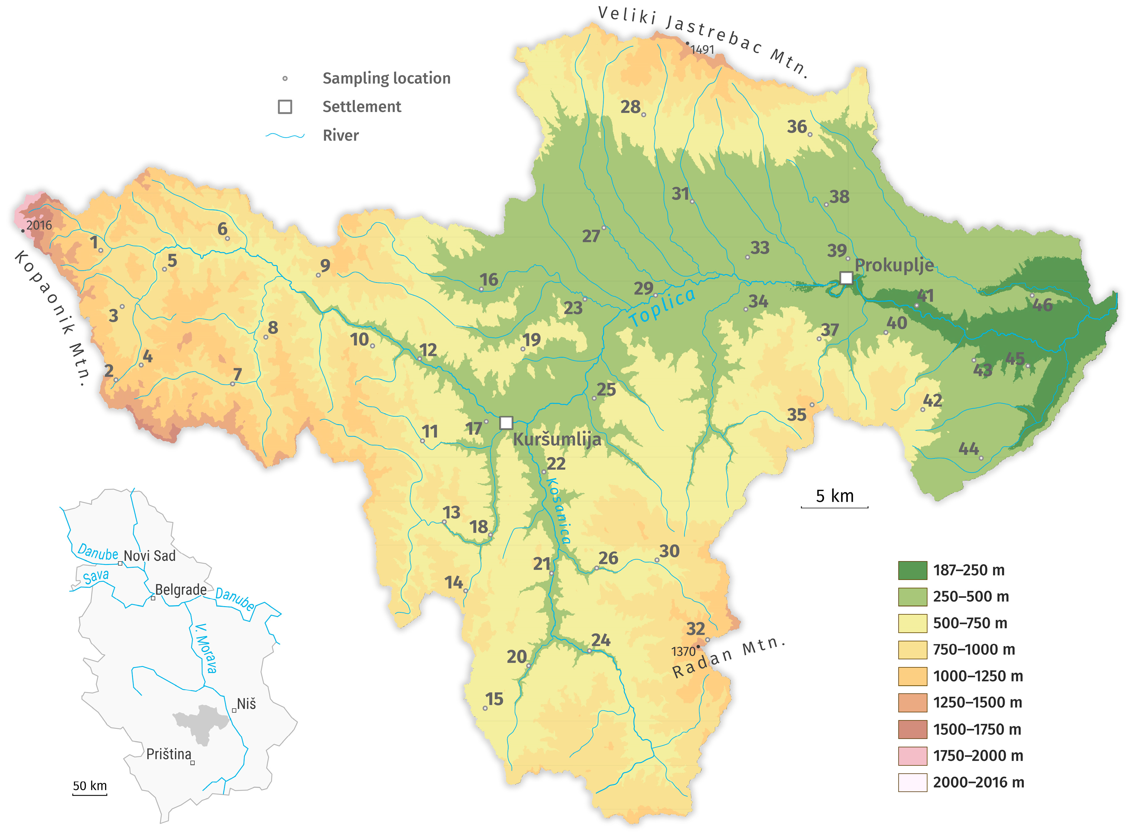
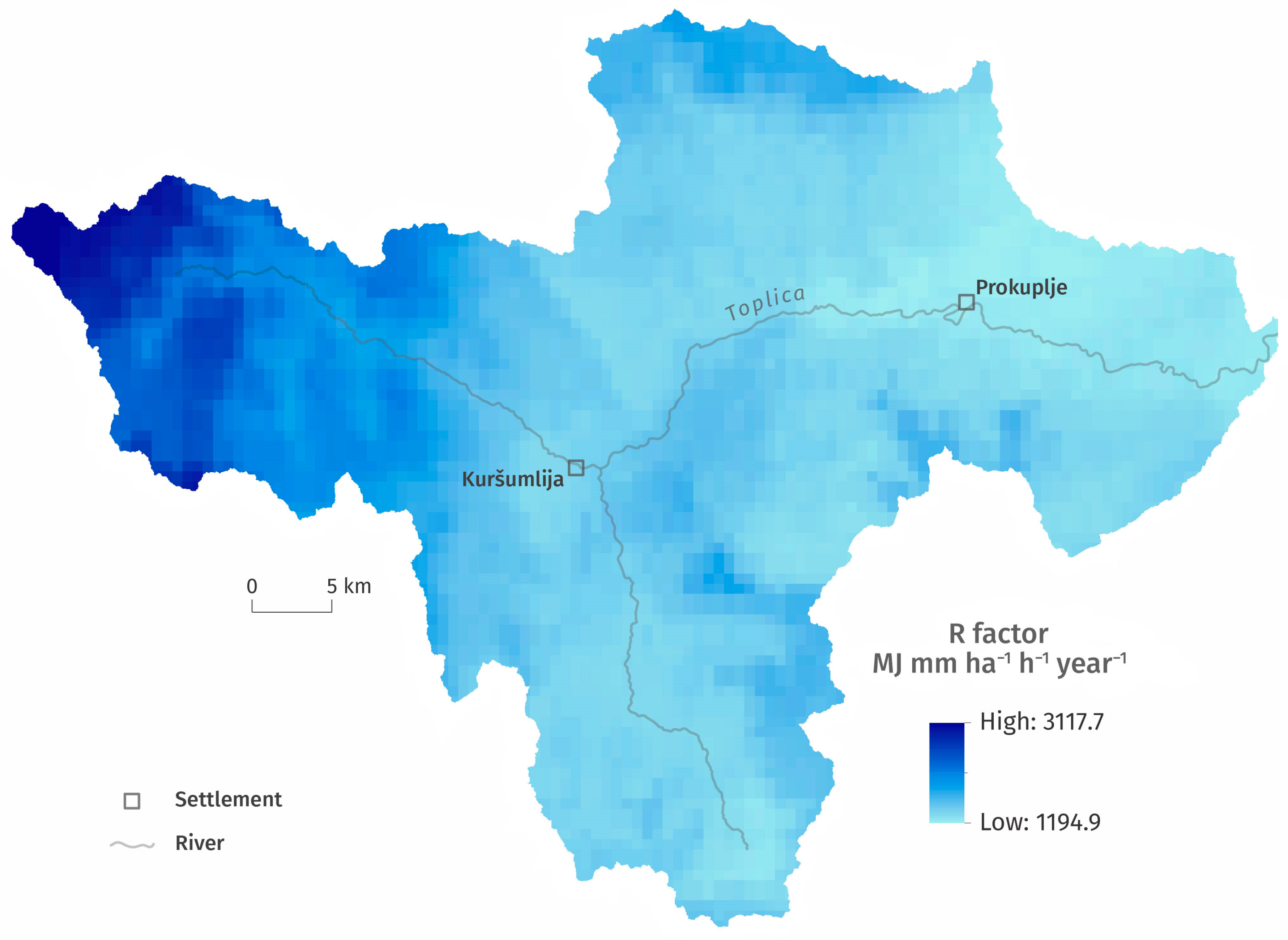
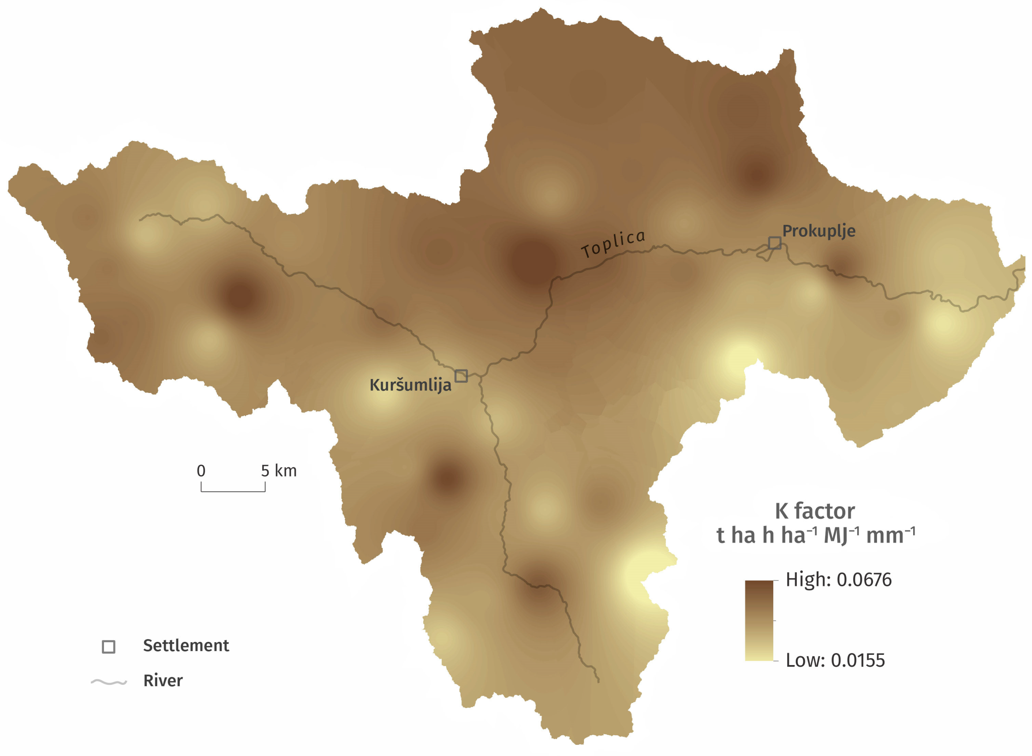
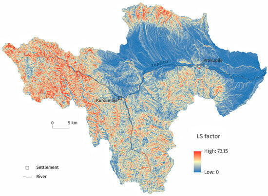
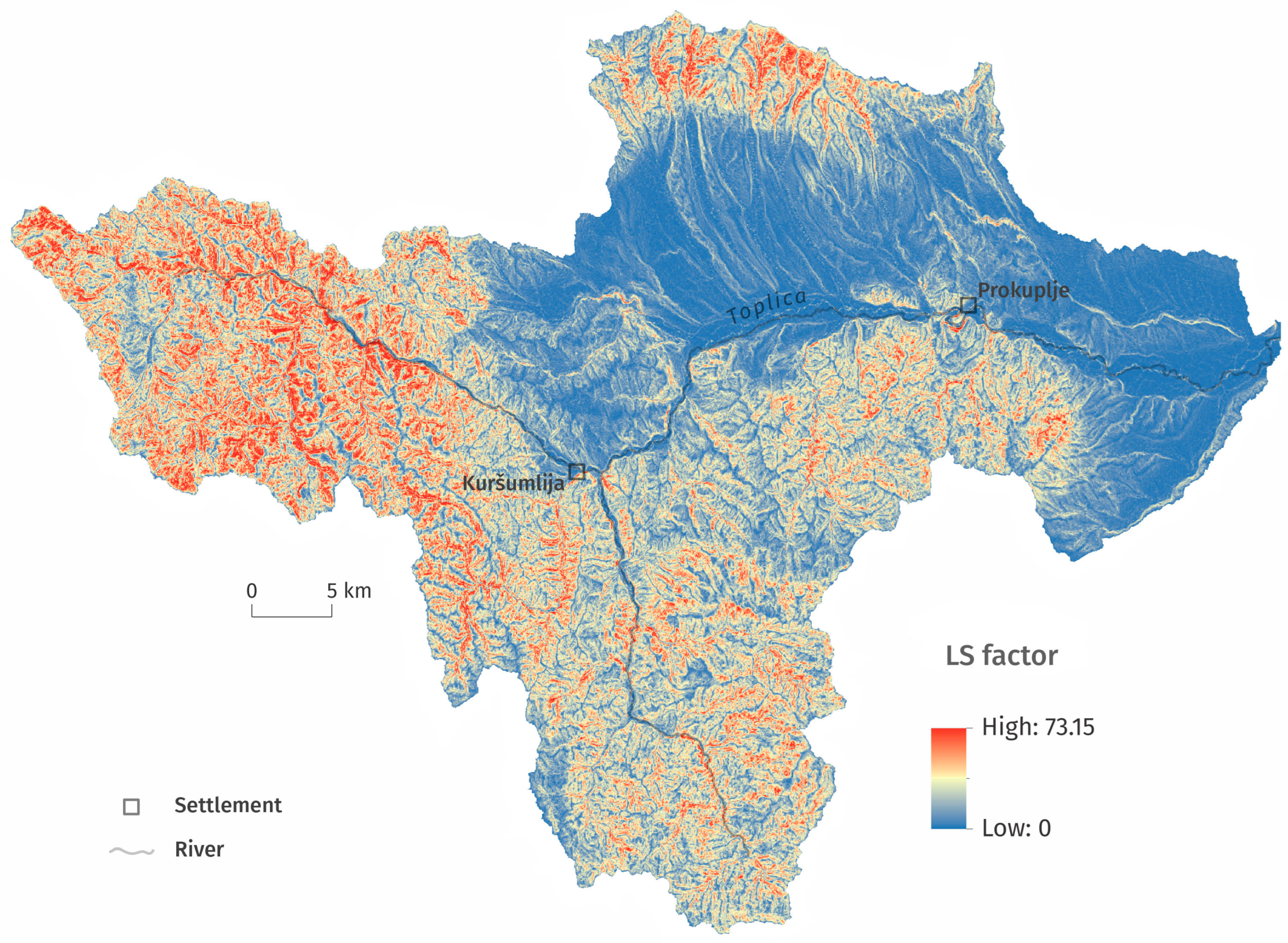
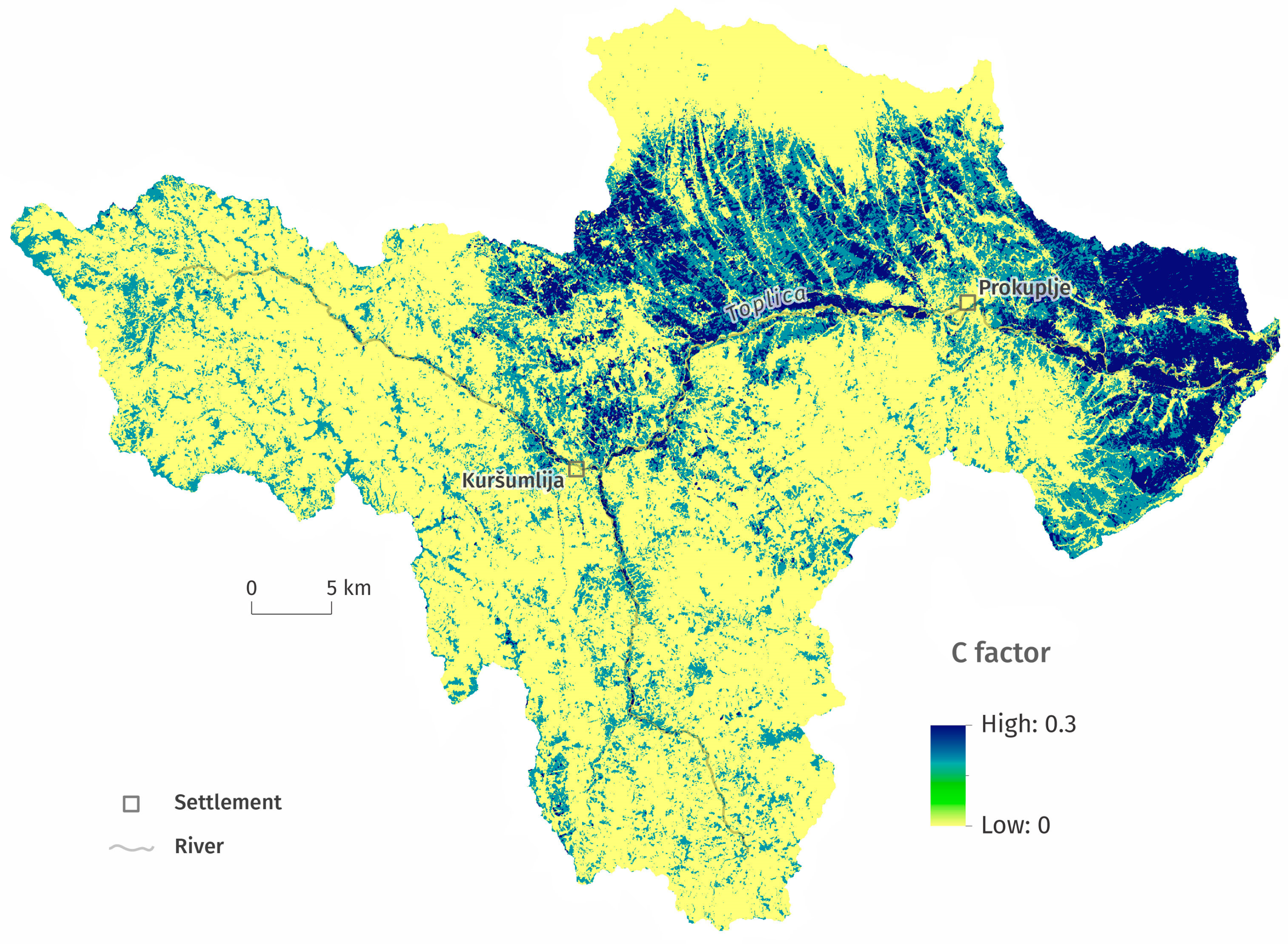
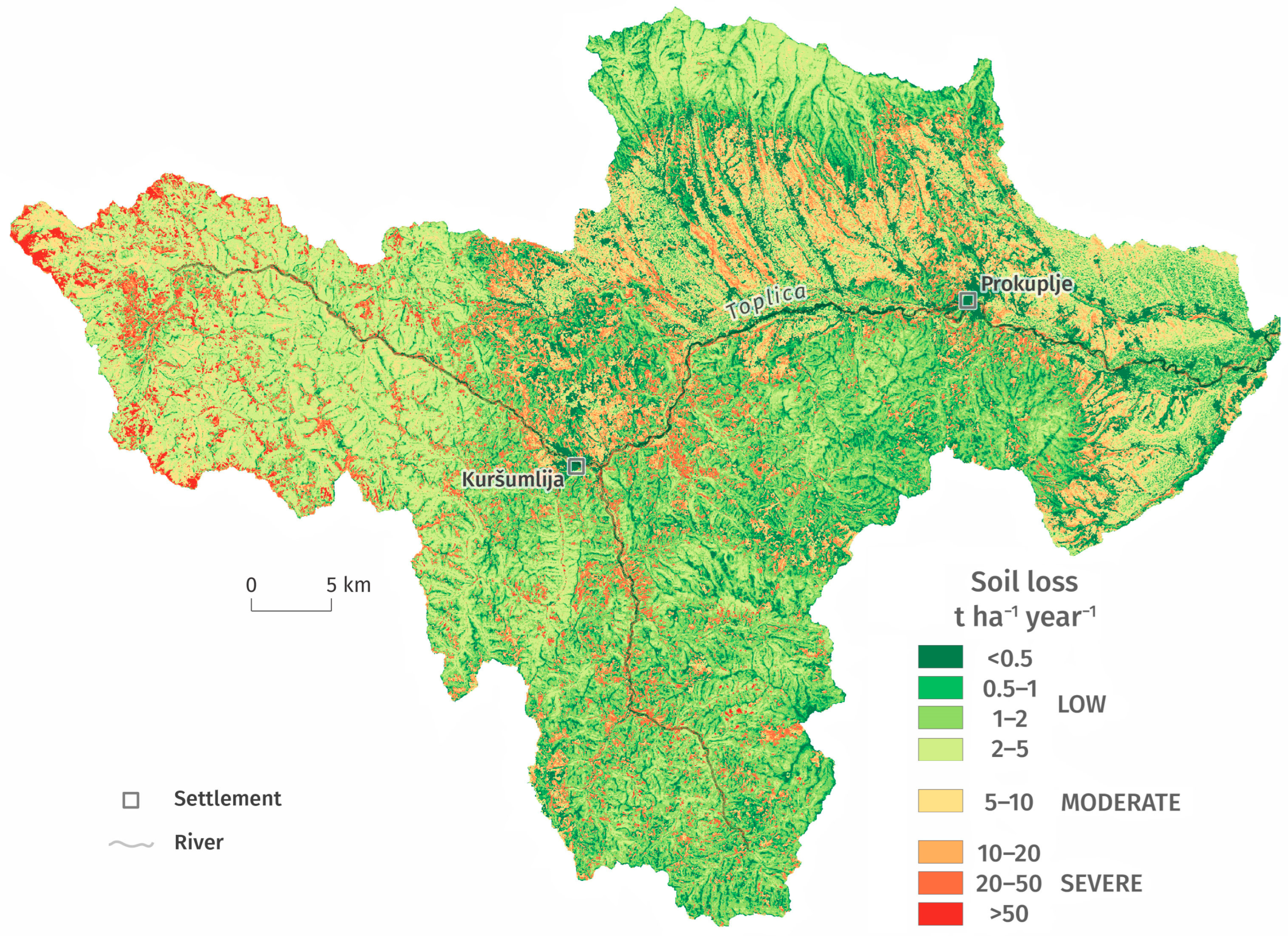

Disclaimer/Publisher’s Note: The statements, opinions and data contained in all publications are solely those of the individual author(s) and contributor(s) and not of MDPI and/or the editor(s). MDPI and/or the editor(s) disclaim responsibility for any injury to people or property resulting from any ideas, methods, instructions or products referred to in the content. |
© 2026 by the authors. Licensee MDPI, Basel, Switzerland. This article is an open access article distributed under the terms and conditions of the Creative Commons Attribution (CC BY) license.