Interpolation of Geological Properties Based on Deep Seismic Attributes

Abstract

Conventional geostatistical methods of spatial interpolation (e.g., inverse distance weighting or kriging) are based on spatial distance and become inaccurate in regions far from sample wells or in the case of geological discontinuities. It looks more natural to estimate geological properties using similarity, not by distance, but by geological conditions, which, in turn, can be estimated using seismic surveys. In this research, we use machine learning to derive seismic attributes that describe the local geological environment and apply interpolation in the resulting attribute space to propagate geological properties from the sample wells to the whole reservoir model. In this representation, geologically similar regions become close in the attribute space even when they are separated in the initial spatial 3D domain. Using an open synthetic dataset, we demonstrate that this approach improves propagation of various geological properties compared to the conventional spatial method and remains effective even with a small number of sample wells. The main advantage of this approach is that, while preserving the simplicity and transparency of geostatistical methods, it enables the use of seismic data without preliminary interpretation to obtain geologically consistent and quick estimates of geological properties in the 3D domain far from sample wells.

1. Introduction

Propagation of geological properties, for example, the propagation of well log data into the inter-well domain, is a common task in geology. It initially arises when the geological model is constructed, and the process is repeated when new data, for example, from new exploratory wells, become available (see, e.g., [1]). When the problem is bounded to the inter-well domain only, i.e., interpolation, and wells are located densely, then the conventional geostatistical interpolation methods (see, e.g., [2]) can be sufficient for a quick estimate. However, they typically fail to propagate properties outside the region where the wells are located, i.e., to extrapolate the data, and one has to involve additional information, e.g., geological structure (see, e.g., [3,4]). If seismic data is available, it can help to improve accuracy in both cases (interpolation and extrapolation), but the question is how to use seismic data efficiently.

The widely used spatial methods are kriging and inverse-distance weighting (IDW). Both methods are essentially linear; the first is based on the assumption of joint normality of the data and allows for uncertainty estimation. The non-trivial parts of the kriging method are selecting and fitting the trend and variogram models, which significantly affect the results. While kriging is a conventional approach in 2D, its application in 3D (e.g., [5]) becomes complicated due to the larger memory consumption for construction of the covariance matrix. One has to consider more efficient approximation methods, e.g., [6,7], and more recent [8,9]. In contrast, the IDW method is much more straightforward for application without significant loss in accuracy (e.g., [10,11,12]), but does not provide uncertainty estimates. In this paper, we will focus on the IDW method in order to avoid problems associated with the application of kriging in high-dimensional space (the proposed method will be used in a space with more than three dimensions) and with selection and estimation of the correlation model.

There are several ways to involve seismic data in the propagation of geological properties. The first approach is known as co-kriging (see review in [13]), in which the estimated variable is modeled as a linear combination of the primary and auxiliary variables at the points where their values are given. The auxiliary variables can be seismic amplitudes or more sophisticated seismic attributes. One can note, however, that knowing the auxiliary variable (seismic data in our case) at the inferred point is not necessary for this method to derive the prediction (auxiliary variables should be known at least at the points that are used for prediction; more data with known auxiliary values only helps to improve covariance and cross-covariance models). This indicates that co-kriging cannot efficiently use information about the auxiliary variable (seismic data). In particular, in [14] it was demonstrated that co-kriging is less accurate than the method that is explicitly based on seismic data at the inferred points.

Another approach is based on seismic inversion. It has a different form and is developed for pre- and post-stack data. Conventionally, it has two steps. The first step is to convert seismic data to acoustic impedance or elastic parameters. In the second step, rock physics and statistical models are used to estimate petrophysical and fluid properties (see, e.g., review in [15]). As is typical for inverse problems, seismic inversion remains computationally intensive, encouraging investigation of alternative approaches. For example, ref. [16] were one of the first to apply neural network models to translate seismic attributes into log properties. Today, deep learning methods are widely investigated; see, e.g., [17,18,19,20,21].

The idea of this paper extends the approach proposed in [14], where the authors measured the distance between points in the reservoir model as the distance between vectors composed of spatial coordinates and seismic attributes and performed kriging based on this distance metric to propagate geological properties. On a set of 2D porosity maps, it was demonstrated that this approach outperforms conventional kriging and co-kriging with seismic attributes.

Our key contribution is that instead of acoustic impedance, which requires seismic inversion, we use a set of seismic features obtained using a machine-learning method directly from seismic amplitudes. By design, this set of features contains complete information about the local seismic structure and does not require seismic inversion. Second, we demonstrate the performance of this approach in 3D rather than in 2D and use a much wider range of geological properties for evaluation. Third, we validate the approach using a synthetic benchmark dataset that allows direct comparison with ground truth and arrange a set of experiments that evaluate both interpolation and extrapolation scenarios.

2. Data and Experimental Setup

We use the open-source Stanford VI synthetic geological model [22] as the benchmark dataset. This model is constructed as an asymmetric anticline filled with a system of channels of decreasing size in deeper layers and representing different sets of facies. In total, the model consists of six million cells arranged in a regular grid of size $150\times 200\times 200$. Cell size is $25\times 25\times 1$ m (depth direction is the last). The stratigraphy is represented by three layers, modeled independently and endowed with different characteristics.

The dataset does not contain seismic data directly, but contains a cube of acoustic impedance. To generate synthetic seismic data, the impedance cube was converted into reflection coefficients calculated as the contrast of acoustic impedance values along the depth axis

$$R_i={\displaystyle \frac{A{I}_{i+1}-A{I}_i}{A{I}_{i+1}+A{I}_i}},$$

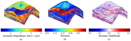
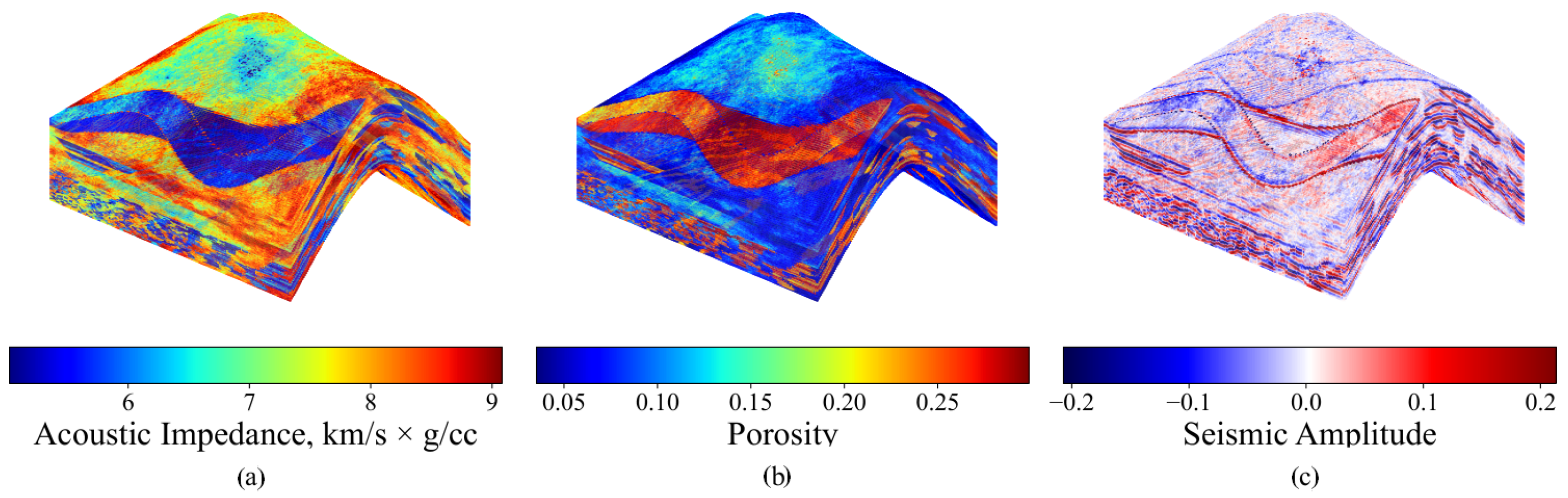
where $A{I}_i$ represents the acoustic impedance at depth level i, and $R_i$ are the derived reflection coefficients. The reflection coefficients were then convolved with a Ricker wavelet with a dominant frequency of 25 Hz and a zero phase. In addition to the acoustic impedance, the dataset contains a set of synthetic petrophysical properties (13 in total, including porosity, permeability, density, seismic P-wave and S-wave velocities, Lame and Poisson coefficients, and initial oil saturation). These arrays are used to evaluate the accuracy of interpolation. Figure 1 shows the geometry of the reservoir model, acoustic impedance, porosity, and generated seismic amplitudes.

Figure 1. Three-dimensional representation of the synthetic reservoir model Stanford VI and values of the acoustic impedance (a), porosity (b), and seismic amplitude generated from the acoustic impedance model (c).

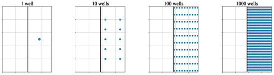
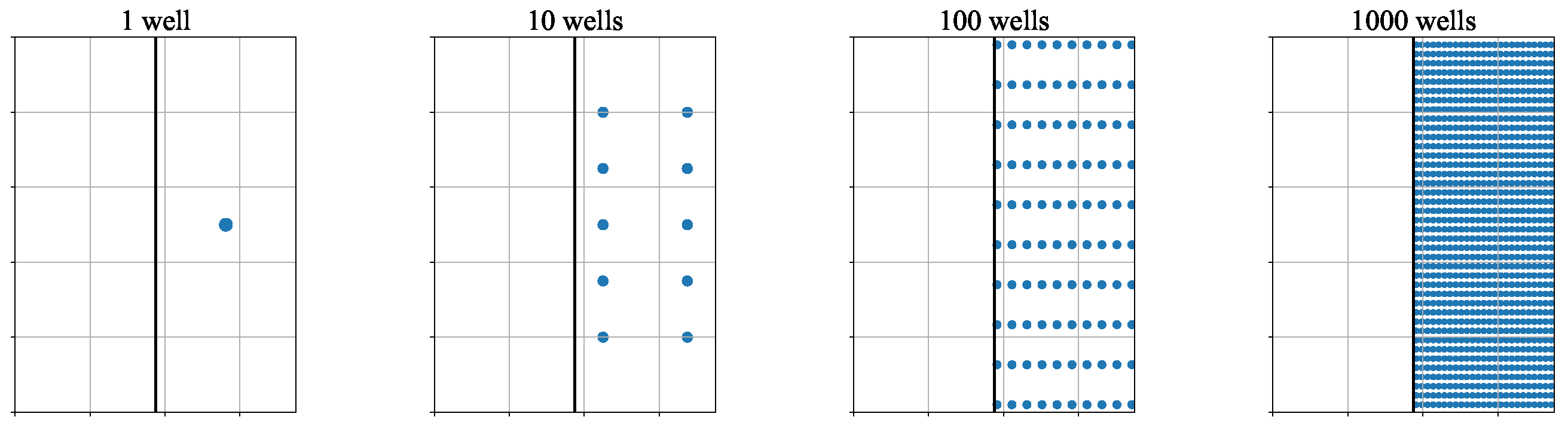
We arrange a set of experiments in which we place a different number of vertical wells (1, 10, 100, and 1000 wells) penetrating the reservoir model from top to bottom in one half of the model (relative to the anticline top). Different numbers of wells are used to investigate how the accuracy of interpolation depends on the number of sample points. The specific location of the well (in one half of the model) will show how the interpolation method works in the domain where no sample points are known (the other half of the reservoir model). Figure 2 shows the location patterns of the sample wells.

Figure 2. Location patterns of the sample wells. The rectangle represents the top view of the reservoir model; the vertical line splits the model into two parts. The wells are located in the right half of the model.

Each well penetrates 200 grid cells and thus provides 200 data points for interpolation of the given property (e.g., porosity, permeability, etc.). The results of interpolation are evaluated on the whole cube using mean squared error (MSE) and $R^2$ (coefficient of determination) metrics. For consistency, all arrays are normalized using min-max scaling based on statistics derived from the training data (sample wells).

3. Methodology

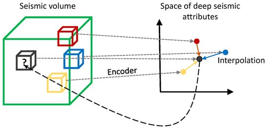
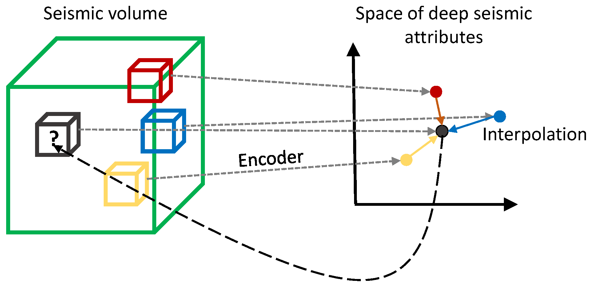
The proposed workflow shown in Figure 3 consists of two main steps: construction of seismic ML attributes and interpolation of well properties using IDW in the resulting feature space. Straightforward IDW interpolation in the initial 3D space is used as a baseline model.

Figure 3. Scheme of the proposed interpolation method. Patches of seismic amplitudes (shown as small boxes; the colors represent the value of the geological property at the patch center) are mapped to seismic attributes using the encoder part of the autoencoder. The geological property is then interpolated in the space of seismic attributes and assigned to the center point of the corresponding patch.

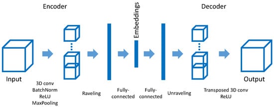
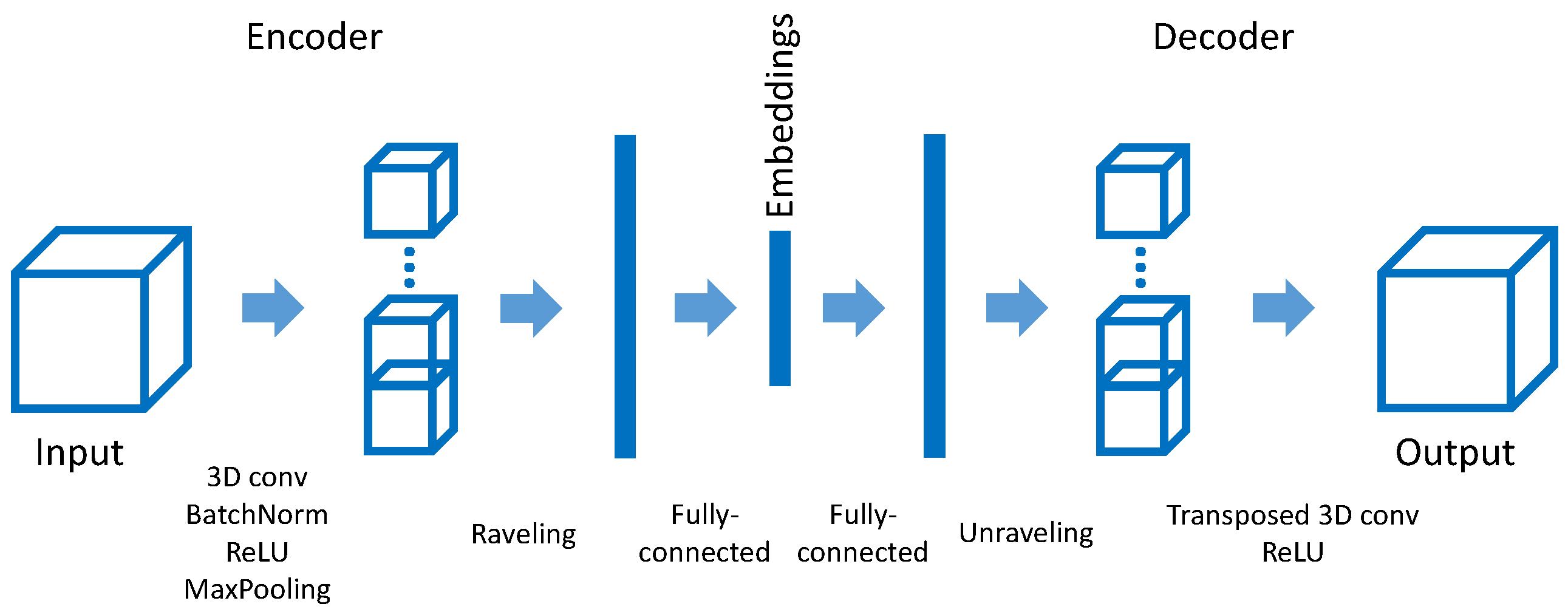
In the first step, a convolutional neural network autoencoder (see, e.g., [23] for general theoretical and practical aspects) is trained to construct seismic attributes that locally describe the geological environment at each point. More specifically, a patch of size $16\times 16\times 16$ grid cells is considered around each cell of the reservoir model. The autoencoder consists of conventional encoder and decoder parts in which 3D convolutions are used. The encoder outputs an array of size eight, considered as the embedding of the given patch. The architecture of the autoencoder is shown in Figure 4. Specifically, the encoder is built as a sequence of three blocks, where each block consists of a 3D convolution with kernel size 3, batch normalization, ReLU activation, and a max-pooling layer. The number of filters in each block doubles and is 32, 64, and 128. After the last block, the output tensor of size $2\times 2\times 2\times 128$ (channel dimension is the last) is flattened and passed to the fully connected layer with an output of size eight, considered as a vector embedding. The decoder is organized in reverse order, and instead of convolutions, transposed convolutions are applied. The autoencoder is trained using the MSE between the input and reconstructed arrays as the loss function. For training, seismic patches were sampled using a sliding window with a stride of one in each direction. Training was performed using the Adam optimizer implemented in Pytorch 2.1.1 [24] with default parameters (including a learning rate of 0.001), with the batch size set to 100, and the number of epochs set to 10. On an NVIDIA Quadro P5000 GPU, the training time was approximately 4 h, with a memory consumption of about 0.3 GB.

Figure 4. Scheme of the autoencoder. The encoder part outputs a vector embedding. The subsequent decoder part is organized in the reverse way.

The key hyperparameter of the autoencoder is the size of the input tensor (3D patch of seismic amplitudes). Smaller patches lead to a more trivial autoencoder, and in the limiting case (a patch consisting of a single cell) the latent vector will just repeat the input seismic amplitude. Larger patches smooth the spatial distribution of the embedding, and it becomes difficult to locate the position of horizons where geological properties change. As a rule of thumb, we propose considering a patch of size 1/10 of the number of cells along the depth axis of the seismic volume. It is also convenient (but not necessary) when the size of the patch is a power of two (this simplifies the down- and upsampling operations in the encoder and decoder parts). For the Stanford VI model, these recommendations yield a patch size of 16 (in each dimension). In order to compress the spatial size of the patch, the number of max pooling layers in the autoencoder should be about ${\log }_{2}D-1$, where D is the size of the patch. For the Stanford VI model, this yields three blocks with max pooling layers.

After training, the encoder part of the autoencoder processes patch-by-patch the full cube of seismic amplitude and assigns an eight-dimensional embedding to each cell of this cube. For a given point a, whose coordinates are ${\overrightarrow{r}}_a=(x_a,y_a,z_a)$, we will denote the embedding as ${\overrightarrow{q}}_a$ (note that its components are dimensionless).

In the second step, geological properties sampled along the well trajectories are interpolated onto the whole reservoir model using the inverse distance weighting [25] method, where the distance between two points a and b of the reservoir model in the baseline model is calculated as the Euclidean distance in the initial three-dimensional space, i.e., $\rho (a,b)=\left|\right|{\overrightarrow{r}}_a-{\overrightarrow{r}}_b\left|\right|$, and in the proposed model the distance is defined as the Euclidean distance between the embeddings ${\overrightarrow{q}}_a$ and ${\overrightarrow{q}}_b$ corresponding to these points, i.e., $\rho (a,b)=\left|\right|{\overrightarrow{q}}_a-{\overrightarrow{q}}_b\left|\right|$.

Due to the overall complexity of the IDW method ($O(n·w)$, where n is the number of points to be interpolated and w is the number of sample points used for interpolation), we use the restricted version of the IDW, in which only k nearest sample points are used for interpolation (the reduced complexity is $O(n·k)$). Formally, to predict a value $\widehat{y}$ at a point ${\mathbf{x}}_0$ given a set of known values $y_i$ at points ${\mathbf{x}}_i$, we use the following equation

$$\widehat{y}\left({\mathbf{x}}_0\right)={\displaystyle \frac{{\sum }_{i\in {\mathcal{N}}_k\left({\mathbf{x}}_0\right)}{w}_i{y}_i}{{\sum }_{i\in {\mathcal{N}}_k\left({\mathbf{x}}_0\right)}{w}_i}},w_i={\displaystyle \frac{1}{\rho {({\mathbf{x}}_0,{\mathbf{x}}_i)}^2}},$$

(1)

where ${\mathcal{N}}_k\left({\mathbf{x}}_0\right)$ denotes a set of k nearest points to the point ${\mathbf{x}}_0$. Note that the distance metric $\rho$ is different in the baseline model and the proposed approach.

The optimal value of k is determined empirically by probing different values and choosing the one that maximizes the interpolation accuracy. Interestingly, as we demonstrate below, the optimal value becomes quite low and much smaller than the maximum possible value of k. Thus, using the restricted IDW not only reduces the time complexity, but also improves the accuracy.

4. Results

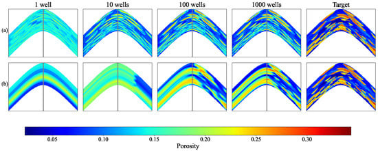
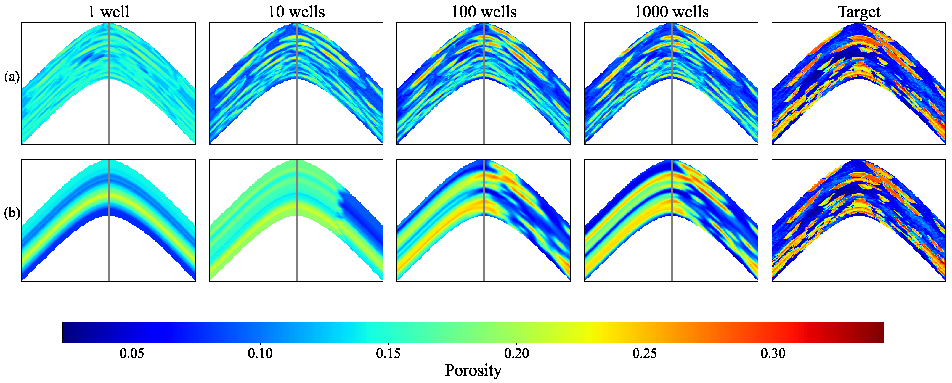
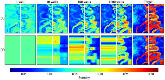
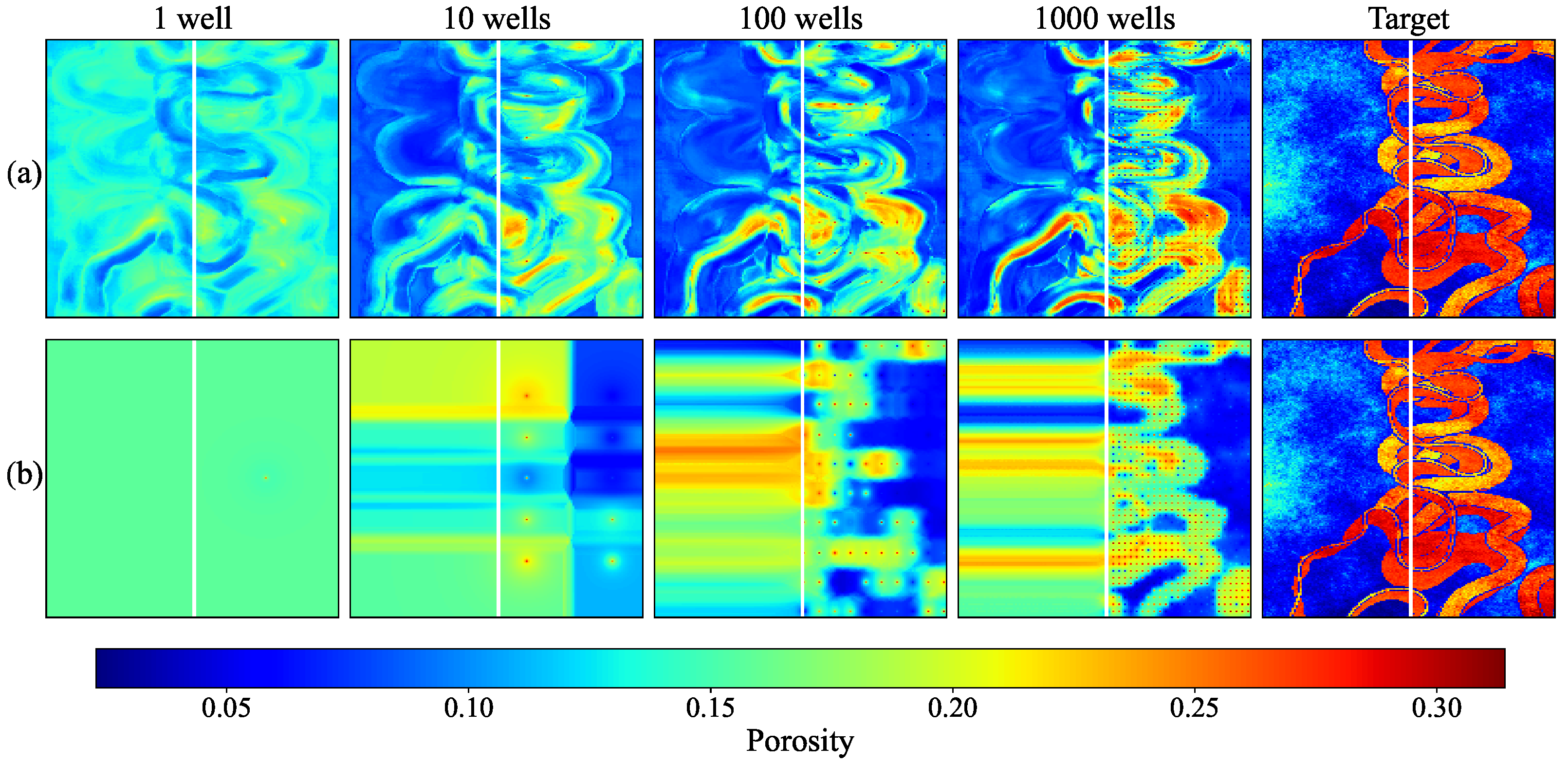
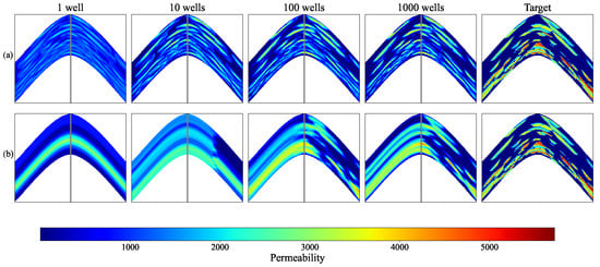
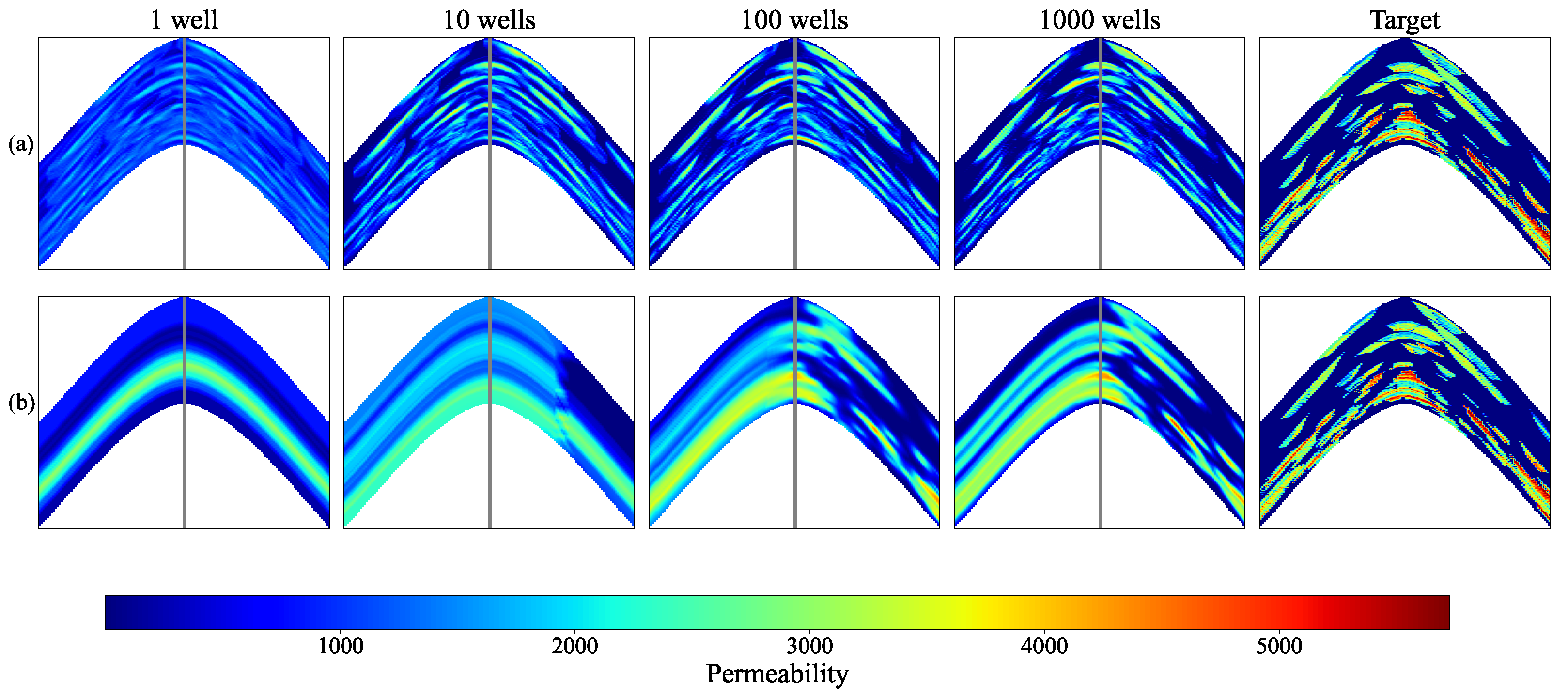
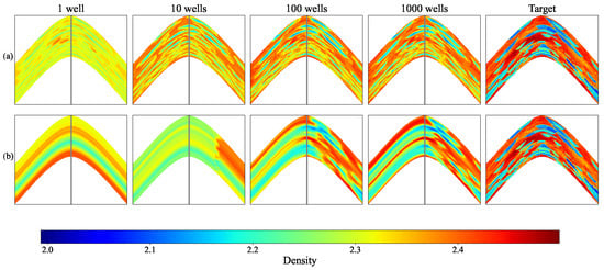
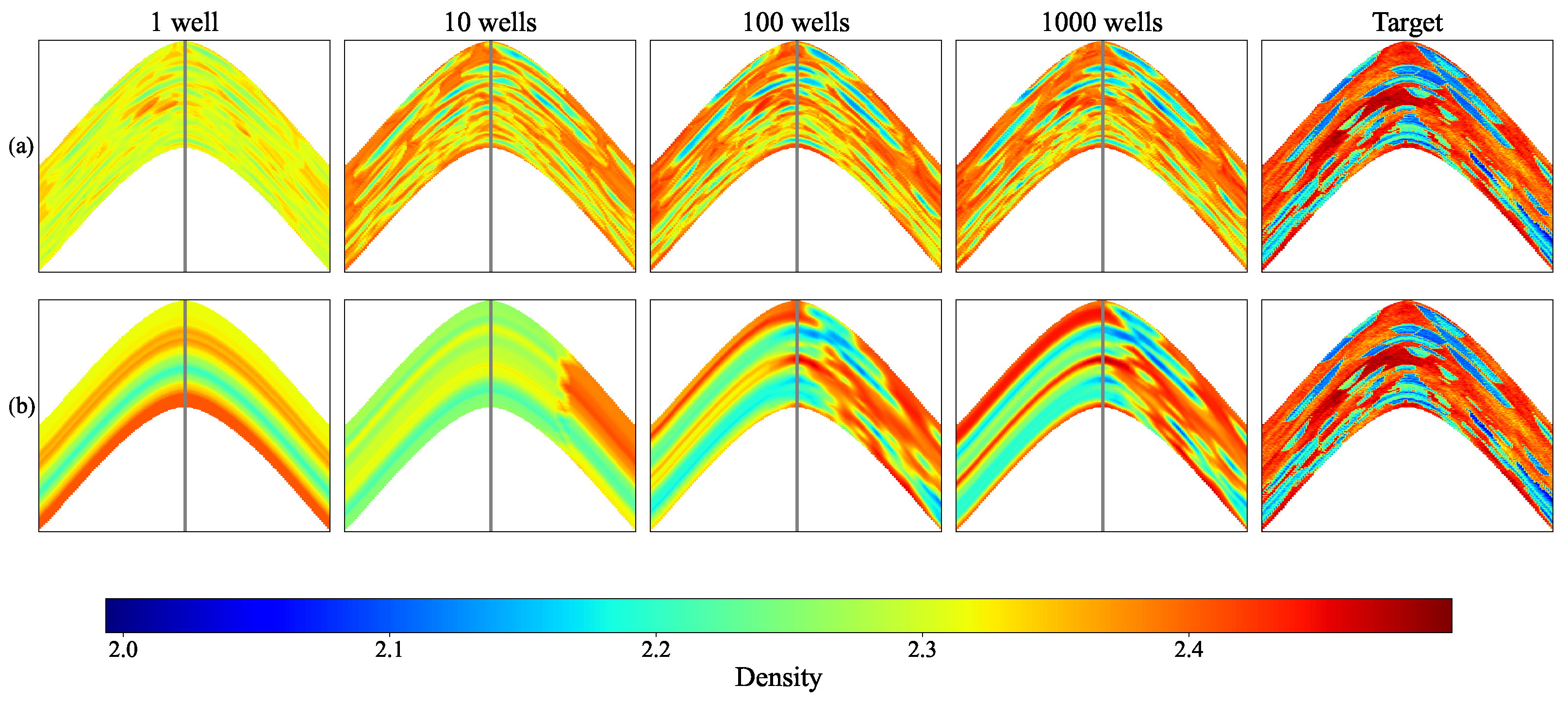
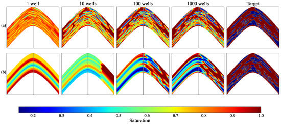
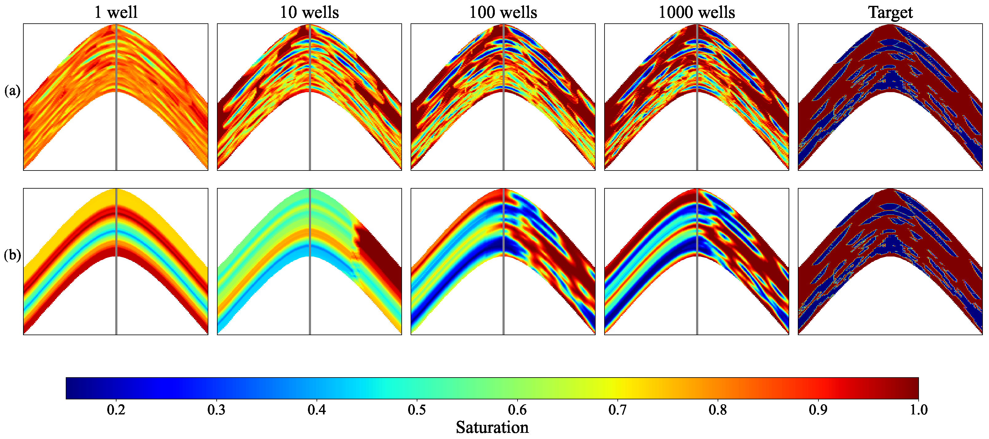
We start with the main result that demonstrates the superior accuracy of the interpolation in the space of the seismic ML attribute compared to the conventional spatial interpolation. Figure 5, Figure 6, Figure 7, Figure 8 and Figure 9 show vertical and horizontal slices of the porosity, permeability, density, and saturation arrays and the results of interpolation from the sample wells located in the right half of the cube onto the whole cube.

Figure 5. Interpolation of the porosity using different numbers of sample wells (the first four columns of subplots for 1, 10, 100, and 1000 wells) and the true values of the porosity (the last column of subplots) for the same vertical slice of the porosity cube. The top row (a) shows the results of IDW interpolation based on the seismic ML attributes. The bottom row (b) shows the results of IDW interpolation based on spatial coordinates. The vertical line in each subplot separates two parts of the reservoir model, and only the right part contains sample wells.

Figure 6. Same as Figure 5 but for a sample horizontal slice.

Figure 7. Same as Figure 5 but for permeability.

Figure 8. Same as Figure 5 but for density.

Figure 9. Same as Figure 5 but for oil saturation.

One can observe in Figure 5, Figure 6, Figure 7, Figure 8 and Figure 9 that the conventional spatial IDW interpolation fails to interpolate the left part of the cube regardless of the number of sample wells in the right part and yields accurate interpolation in the right part only when the sample wells are located densely. Actually, predicting values in the left part of the cube given sample data in the right part using spatial methods is extrapolation rather than interpolation. In this respect, it is natural that the spatial IDW method leads to constant values when extrapolated.

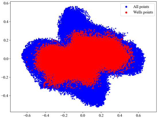
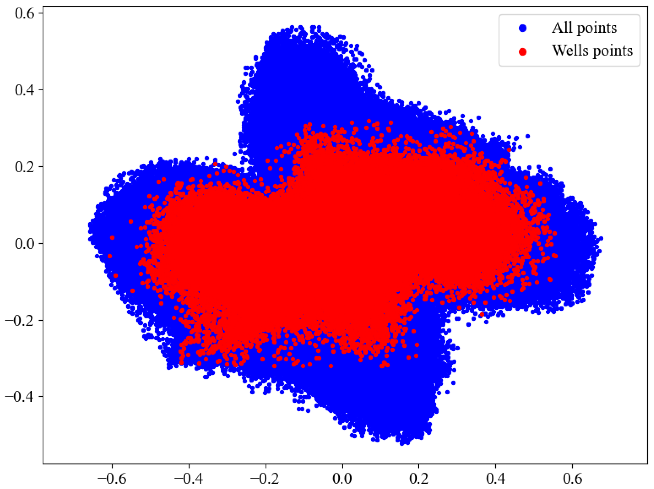
In contrast, we argue that in the space of seismic ML attributes, predicting values in the left part of the cube given sample data in the right part is interpolation rather than extrapolation. To demonstrate it, we project the embeddings onto the 2D plane using the principal component analysis algorithm and show projections of the sample points and the rest points (from the whole cube) using different colors in Figure 10. One can observe that both sets of points are distributed in the same domain, indicating that in the embedding space the left and the right part of the seismic cube are indistinguishable (this situation is shown schematically in Figure 3). This result explains why the IDW method based on seismic ML attributes successfully predicts values in the left part of the cube, as shown in Figure 5, Figure 6, Figure 7, Figure 8 and Figure 9.

Figure 10. PCA projection of the seismic embeddings. Blue dots correspond to the points from the whole seismic cube; red dots correspond to points along the well trajectories.

One more important observation in Figure 5, Figure 6, Figure 7, Figure 8 and Figure 9 is that the IDW method applied in the space of seismic ML attributes requires much fewer sample points to provide reasonable predictions compared to the spatial IDW interpolation. In fact, even a single well is sufficient to reconstruct the porosity distribution pattern, whereas in the case of spatial IDW interpolation, a single well provides just a constant prediction in each layer of the model (which is quite expected).

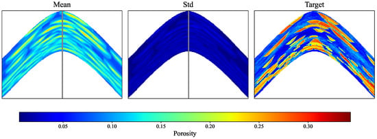
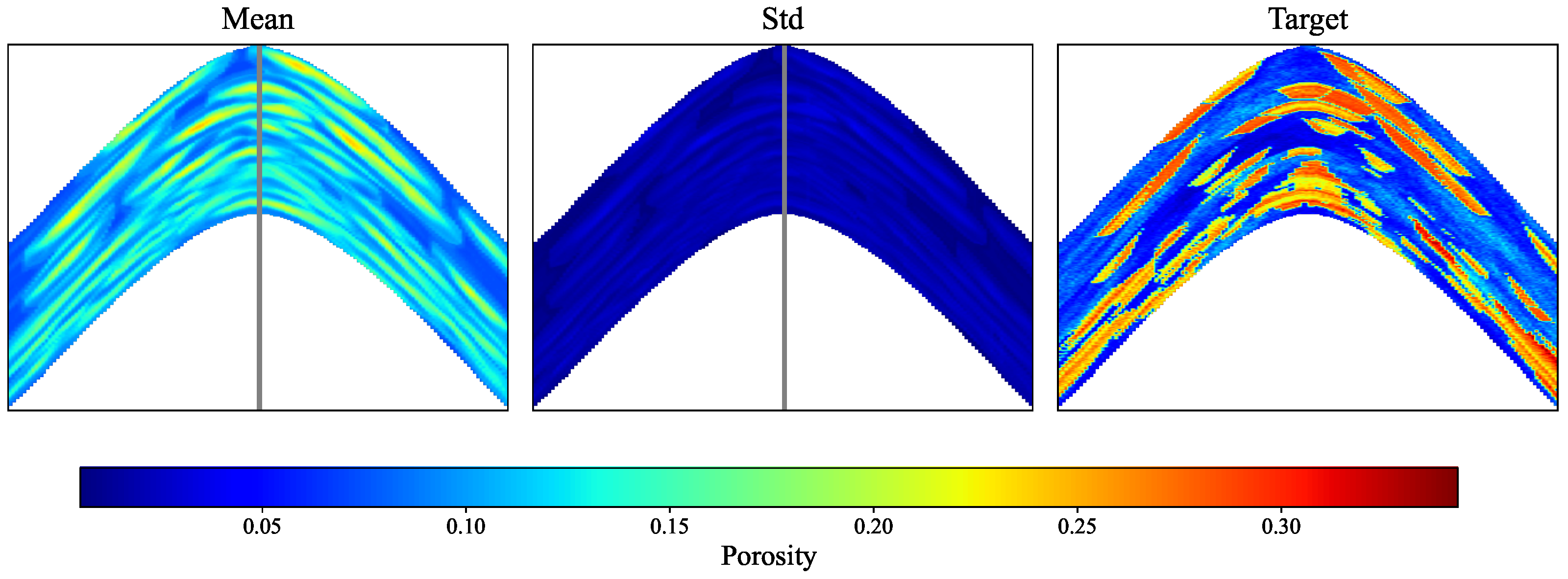
In order to estimate the influence of well location pattern, we performed a test in which 10 wells were located randomly (also in the right part of the model) and the porosity was interpolated using the deep seismic attributes. This test was repeated for 100 independent realizations of well locations, and Figure 11 shows the mean value and standard deviation of the interpolated porosity. We observe that, quantitatively, the results are in agreement with what we observe in Figure 5 for the regularly spaced wells.

Figure 11. Averaged value (left panel) and standard deviation (middle panel) of interpolated porosity (using the deep seismic attributes) based on 100 independent realizations of the random placement of 10 wells. (Right panel) shows the actual porosity values.

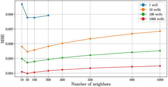
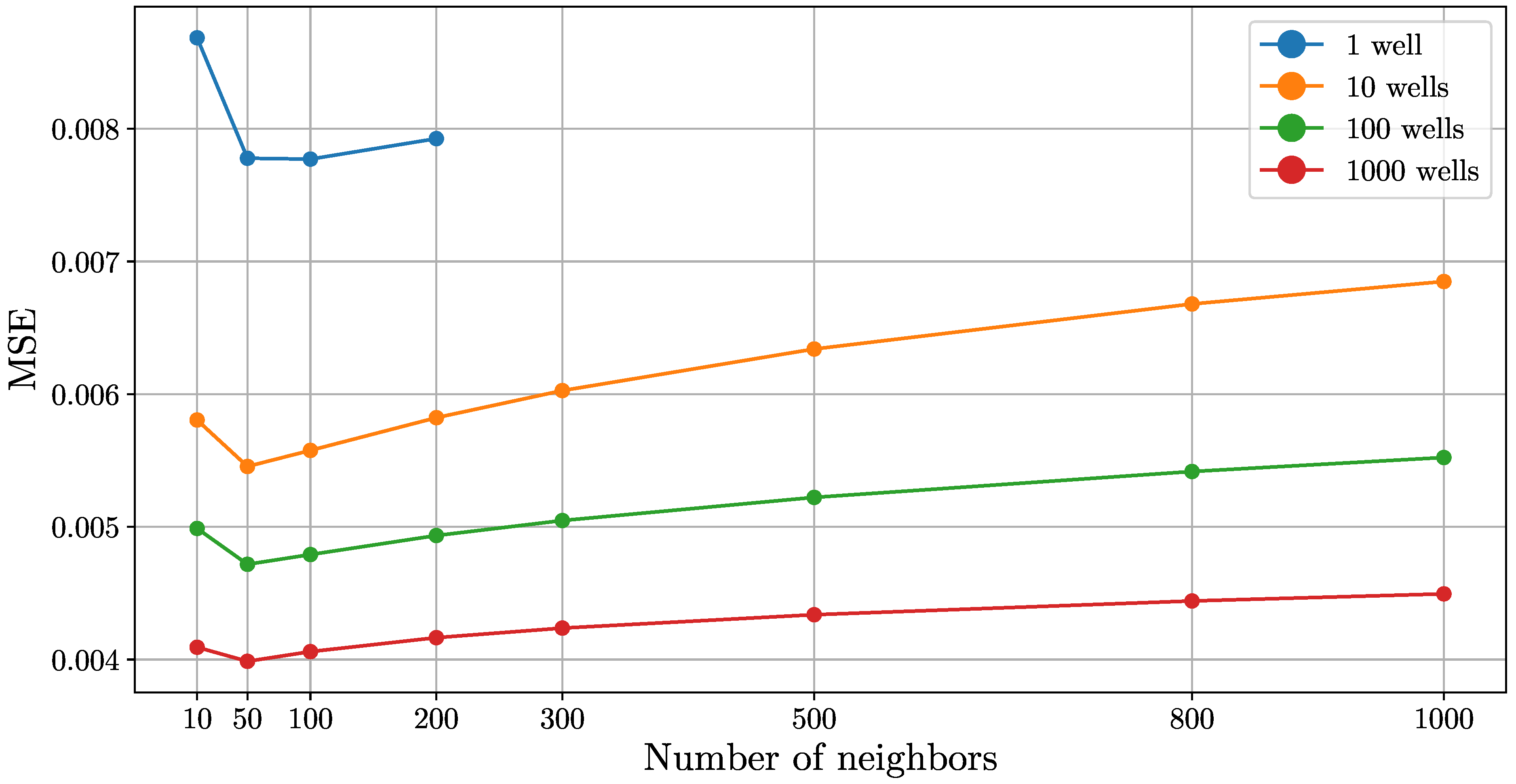
In the above experiments, we use constrained IDW method that takes into account only 50 nearest data points. Now we validate this choice. Figure 12 shows MSE for predicted porosity values in the whole cube using different numbers of nearest neighbors. We observe that regardless of the number of sample wells, the MSE metric is minimized when the number of neighbors is about 50. This result is a bit surprising. A natural expectation is that the larger the number of data used, the better the accuracy. In fact, a large number of neighbors leads to smooth results, while the ground-truth data has sharp boundaries.

Figure 12. MSE of the predicted porosity in the whole cube against the number of nearest neighbors used in the IDW method. Different colors correspond to different numbers of sample wells.

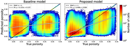
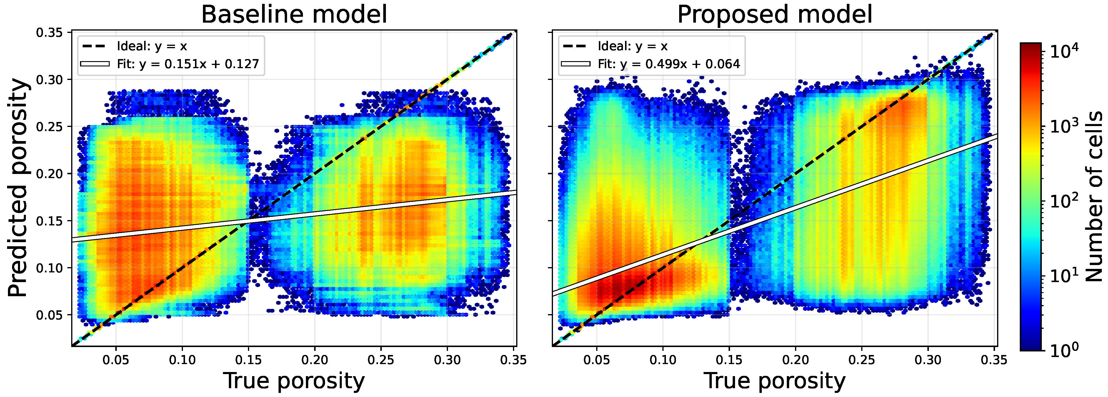
Figure 13 shows the joint distribution of true and predicted porosity values interpolated using the spatial IDW method and IDW interpolation in the space of ML attributes (in both cases, 1000 wells were used as sample data). Although both methods yield a wide spread of predicted values, the distribution for the proposed model is more concentrated around the diagonal line, and the slope of the regression line is closer to 1.

Figure 13. Histogram of predicted and true porosity values for the spatial IDW interpolation (baseline model, left panel) and the IDW interpolation in the space of ML attributes (proposed model, right panel).

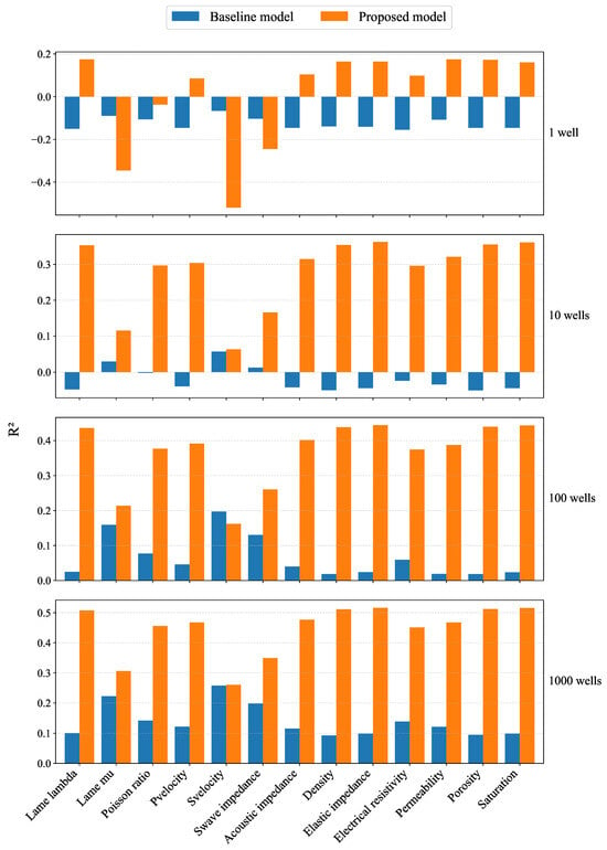
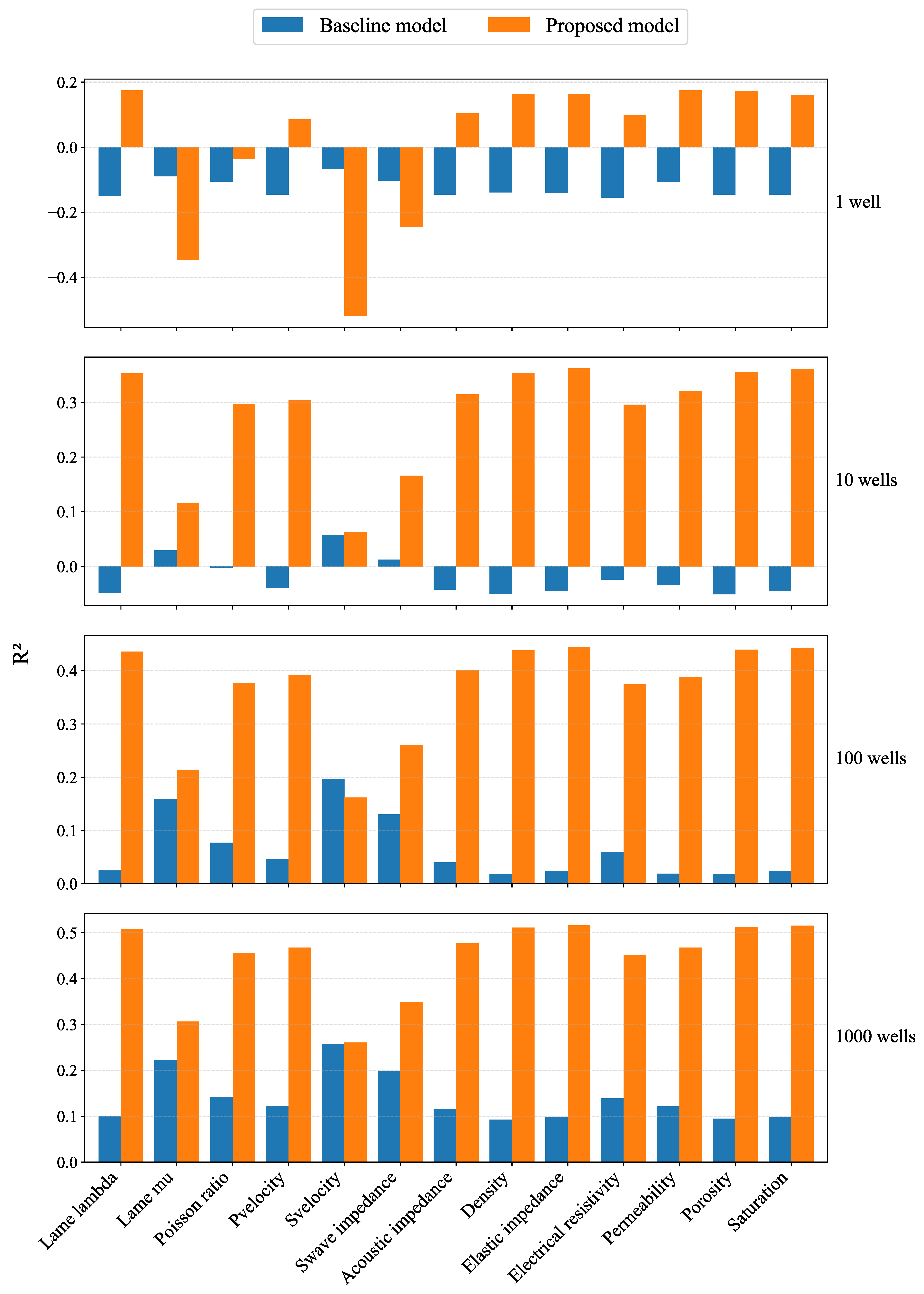
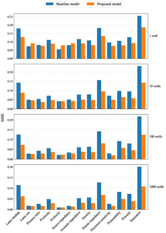
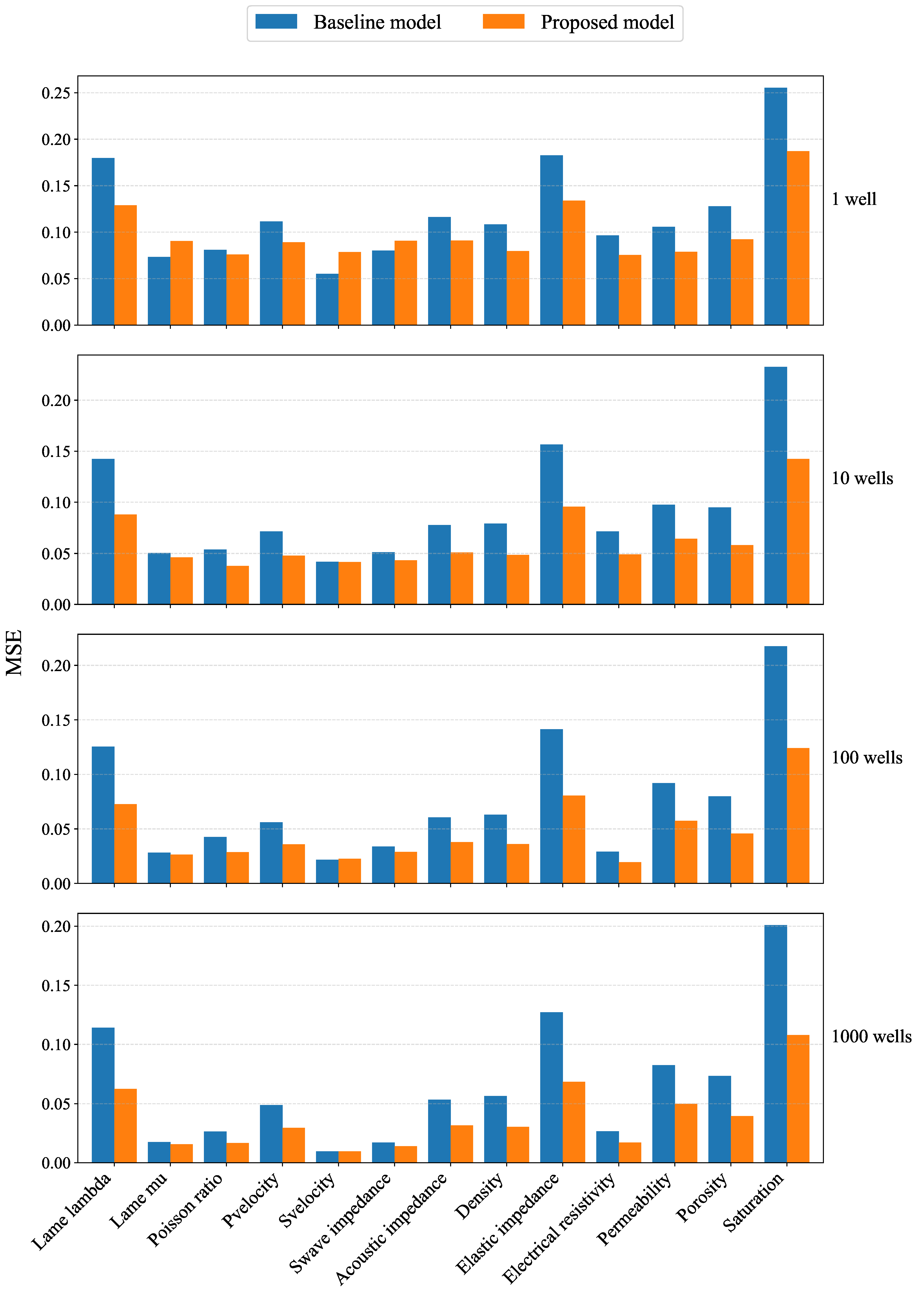
Finally, we demonstrate that the results obtained above remain valid for the other geological properties. Figure 14 and Figure 15 show $R^2$ and MSE metrics for the baseline interpolation model and the proposed one on the whole set of geological properties presented in the Stanford-VI dataset. It can be seen that the proposed approach provides uniformly better results of interpolation for all rock mechanical properties and saturation and for any number of sample wells.

Figure 14. $R^2$ metric for predicted geological properties in the whole cube. Blue bars correspond to the conventional spatial interpolation, orange bars are the interpolation in the space of seismic embeddings.

Figure 15. MSE metric for predicted geological properties in the whole cube. Blue bars correspond to the conventional spatial interpolation, orange bars are the interpolation in the space of seismic embeddings.

5. Discussions

This study proposed a seismic-guided approach to propagating well data in the whole reservoir domain. Importantly, this approach does not require preliminary picking of seismic horizons, similar to the predictive-painting method (see [26]). A convolutional autoencoder was used to construct seismic ML attributes that characterize the local geological environment. The difference between the obtained attributes was used as a distance metric between points in the reservoir domain. Based on this distance metric and the known geological properties along the wells, the geological properties at the remaining points were predicted using the IDW algorithm. Conventional spatial propagation based on the IDW algorithm (using the distance between the spatial coordinates) was considered as the baseline model.

The experiments on a synthetic geological model showed that replacing spatial distances with distances between learned seismic representations uniformly improves propagation of various geological properties. The experiments allowed estimation accuracy of both interpolation and extrapolation scenarios. The most significant difference was observed in the extrapolation scenario. While the conventional spatial IDW method, as expected (see, e.g., [27]), failed to provide reasonable predictions outside the domain where the sample wells were located, the IDW method based on deep seismic attributes yielded accurate results. Remarkably, for the proposed method, even a single well was enough to predict a reasonable pattern of the geological property distribution in the regions far from this well, while the conventional IDW method led to layered constant values.

When the data were interpolated (rather than extrapolated), the difference with the baseline method was also significant. The proposed method required much fewer sample wells to give reasonable results. Even with the maximum number of wells, although the results appear visually similar, the proposed method still demonstrates better qualitative metrics.

The problem of the correspondence between the visual results and formal metrics is in fact non-trivial. Looking at the slices of predicted properties (e.g., Figure 5, Figure 6, Figure 7, Figure 8 and Figure 9) one can clearly note the difference between the both methods. The most prominent difference is in the left part of the model, where the proposed method reconstructs the geological structure, although the amplitudes may not be exact, while the baseline methods fail to reconstruct even the geological structure. A similar situation is observed for a low number of wells in the right part of the model. However, looking at the MSE metrics, the difference appears to be not as dramatic. For example, for porosity, MSE for the baseline model is only twice as high as the MSE of the proposed model. The contrast in the $R^2$ metrics is more pronounced. For example, for porosity it is 0.1 for the base model and 0.5 for the proposed model at 1000 wells, and for the base model it even becomes negative at one well. However, one could argue that 0.5 is still a moderate value for $R^2$. Our conclusion from this case is that the standard metrics do not provide adequate support for perceptual quality control. Apparently, more advanced metrics, such as structural similarity indices [28] should be adopted for evaluation of spatial interpolation.

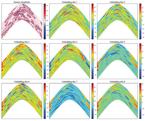
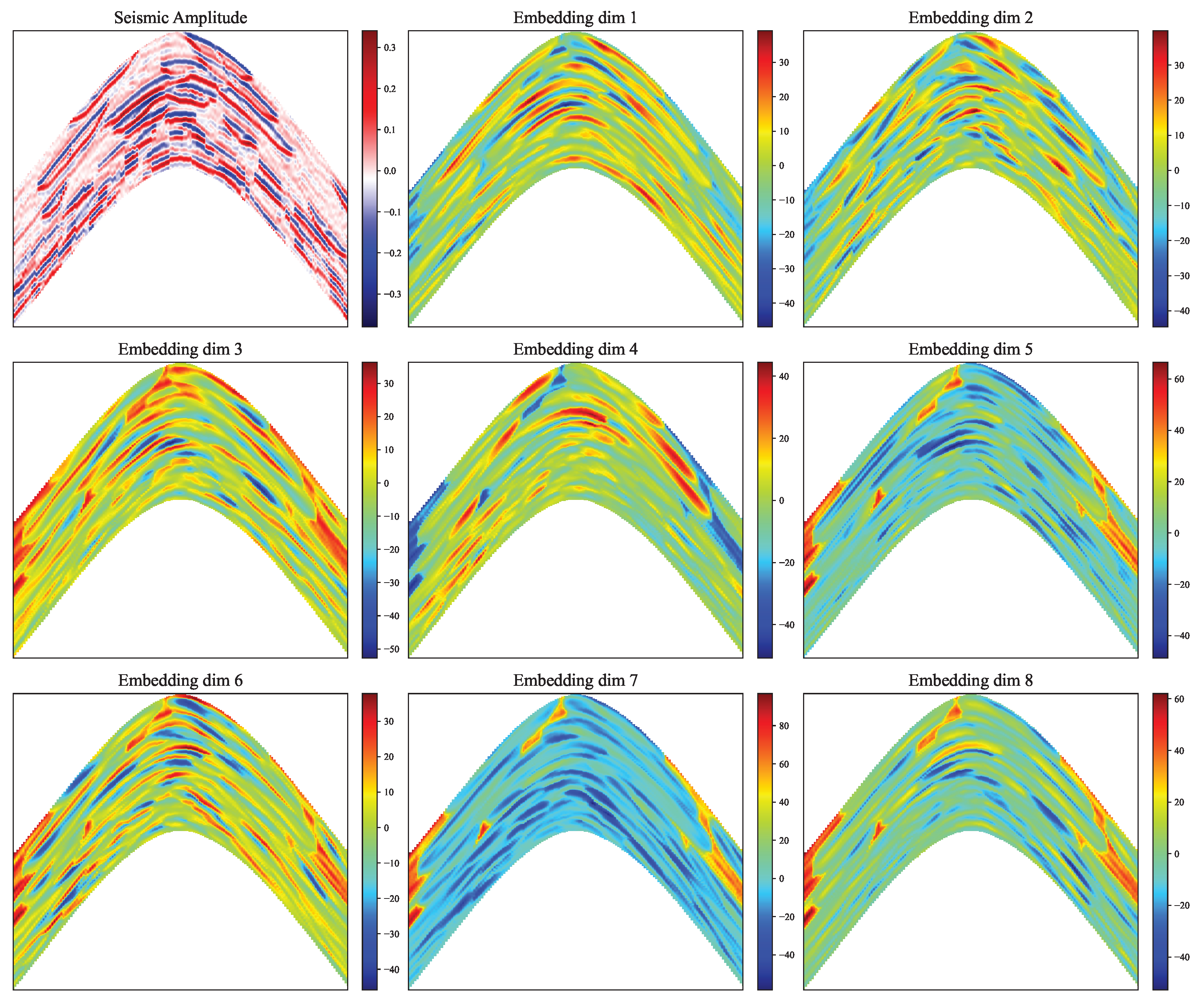
To discuss the physical interpretation of the embeddings, consider Figure 16, in which slices of the cubes of embeddings are compared with the corresponding slice of the cube of seismic amplitudes. One can note that the embeddings do not reproduce seismic amplitudes directly. In contrast, some embeddings, e.g., in dimensions 1, 3, and 4, capture large-scale structures, while embeddings in dimensions 2 and 6 capture rather small-scale structures. Embeddings in dimensions 5, 7, and 8 are most activated in regions of low seismic amplitudes. Thus, we consider the obtained embedding as generic features describing the local geological structure, and these features look more informative for estimation of geological properties in comparison to the seismic amplitudes themselves. Additional terms and constraints in the loss function of the autoencoder can be used to configure the latent space of the autoencoder and provide it with more specific physical meaning (see, e.g., physics-informed autoencoder [29]).

Figure 16. Slice of seismic amplitudes and corresponding slices of the embedding cubes.

The limitations of the proposed model follow directly from its design but still should be noted. First, the model is not sensitive to the nature of the geological property. Thus, the properties that are more correlated with seismic properties are expected to be interpolated more accurately compared to the properties that are less correlated with seismic properties, e.g., fluid properties (see, e.g., [30] for a review of the problem). Second, the autoencoder model trained on a particular seismic dataset is not expected to be accurate on another dataset. At the moment, training a new model for a new dataset looks more pragmatic than creating a universal model. However, modern foundation machine-learning models (see, e.g., [31]) havee the potential to change this point of view. Third, the simple autoencoder lacks a number of symmetries that look physically relevant. For example, rotation of the input tensor along the vertical axis can change the latent representation if the values in the tensor are not rotationally invariant. Addressing this issue will lead to even more useful embeddings that are sensitive to the seismic pattern only and not sensitive to the orientation (see, e.g., [32,33] for possible approaches). Actually, an autoencoder is only one way for the embeddings to be derived, and there are a number of other machine-learning approaches, for example, based on contrastive and self-supervised approaches (see, e.g., [34] for a review). Fourth, the specific parameters of the autoencoder model, the patch size, and other settings are not universal and were selected during a set of experiments (finer optimization is still possible but is out of the scope of this paper). There is also room for optimization of the computational performance. The main bottleneck is the training and inference of the autoencoder. For the dataset investigated, these processes took several hours of computational time. In contrast, the computational time for IDW interpolation with a limited number of neighbors is almost negligible. Fifth, implementation of the proposed approach requires specific frameworks that are beyond typical geological software, as well as collaboration between machine learning specialists and geologists.

We demonstrated the approach using the synthetic dataset only. On the one hand, it allowed arranging a number of experiments with different well locations and geological properties and, most importantly, with known ground truth. We realize that real-world data are more challenging. At the same time, we believe that the core idea described in this paper is generally more valuable than its implementation for a specific dataset, which requires discussing a large number of details (data quality, seismic migration, etc.) that distract from the essence of the solution. Moreover, unfortunately, we were unable to find a proper open-source real-world dataset that could be directly used for evaluation, i.e., containing a large number of wells where well log data would be available and interpreted (e.g., porosity estimated), and seismic data would already be migrated in the depth domain and cover the entire well asset.

We hope that the methodological simplicity and physical transparency of the proposed method will encourage its practical implementation and future development. For example, one of the natural applications is prediction of mud-weight window based on interpolated rock mechanical properties (see, e.g., [35]) and quick update of geological models based on new well logs and seismic data.

6. Conclusions

The key conclusions of this research are:

• Using seismic attributes, the problem of 3D spatial interpolation and, importantly, extrapolation was reduced to the problem of interpolation in the space of seismic attributes, justifying the application of conventional geostatistical method of interpolation (e.g., IDW);
• Rather than deriving seismic attributes explicitly, a machine-learning model can be trained to map data into compact and informative embeddings;
• Seismic attributes were derived from local context windows, and the size of the window is a compromise between accuracy of localization of geological boundaries and ability to relate seismic data to geological properties;
• In the synthetic model, the proposed approach outperformed the conventional 3D spatial interpolation, most significant improvements were observed in regions far from sample wells; based on the results in Figure 15, the MSE metrics were reduced by up to two times;
• In the regions between the sample wells, the proposed approach required fewer sample wells compared to the conventional spatial interpolation to get similar accuracy.

We consider this approach as an intermediate tool between the simplest spatial interpolation and more advanced methods requiring preliminary seismic interpretation, and we expect that it will help to improve the accuracy of the seismic inversion and provide a quick and geologically consistent outlook of the subsurface environment.

References

- Fletcher, S.J. Data Assimilation for the Geosciences: From Theory to Application, 2nd ed.; Elsevier: Amsterdam, The Netherlands, 2022. [Google Scholar]
- Azevedo, L.; Soares, A. Geostatistical Methods for Reservoir Geophysics; Springer: Cham, Switzerland, 2017. [Google Scholar] [CrossRef] [Scilit]
- Chen, Y.; Chen, H.; Xiang, K.; Chen, X. Geological structure guided well log interpolation for high-fidelity full waveform inversion. Geophys. J. Int. 2016, 207, 1313–1331. [Google Scholar] [CrossRef] [Scilit]
- Chen, H.; Gao, B. Well-log interpolation with relative geological time constraints for poststack seismic inversion. Acta Geophys. 2026, 74, 226. [Google Scholar] [CrossRef] [Scilit]
- Olkhovikov, A.; Koroteev, D.; Antipova, K. Kriging Is All You Need to Obtain Rock Mechanical Properties From Sparse Spatial Data. Spe J. 2025, 30, 2269–2284. [Google Scholar] [CrossRef] [Scilit]
- Smola, A.; Bartlett, P. Sparse Greedy Gaussian Process Regression. In Proceedings of the Advances in Neural Information Processing Systems, Denver, CO, USA, 27 November–2 December 2000; Volume 13. [Google Scholar]
- Titsias, M. Variational Learning of Inducing Variables in Sparse Gaussian Processes. In Proceedings of the Twelfth International Conference on Artificial Intelligence and Statistics, Clearwater Beach, FL, USA, 16–18 April 2009; Volume 5, pp. 567–574. [Google Scholar]
- Pleiss, G.; Gardner, J.; Weinberger, K.; Wilson, A.G. Constant-Time Predictive Distributions for Gaussian Processes. In Proceedings of the 35th International Conference on Machine Learning, Stockholm, Sweden, 10–15 July 2018; Volume 80, pp. 4114–4123. [Google Scholar]
- Wilson, A.G.; Nickisch, H. Kernel Interpolation for Scalable Structured Gaussian Processes (KISS-GP). arXiv 2015, arXiv:1503.01057. [Google Scholar]
- Fu, T.; Gao, H.; Liu, J. Comparison of Different Interpolation Methods for Prediction of Soil Salinity in Arid Irrigation Region in Northern China. Agronomy 2021, 11, 1535. [Google Scholar] [CrossRef] [Scilit]
- Otchere, D.A.; Hodgetts, D.; Ganat, T.A.O.; Ullah, N.; Rashid, A. Static Reservoir Modeling Comparing Inverse Distance Weighting to Kriging Interpolation Algorithm in Volumetric Estimation. Case Study: Gullfaks Field. In Proceedings of the Offshore Technology Conference, Houston, TX, USA, 16–19 August 2021. [Google Scholar] [CrossRef] [Scilit]
- Boumpoulis, V.; Michalopoulou, M.; Depountis, N. Comparison between different spatial interpolation methods for the development of sediment distribution maps in coastal areas. Earth Sci. Inform. 2023, 16, 2069–2087. [Google Scholar] [CrossRef] [Scilit]
- Dowd, P.A.; Pardo-Igúzquiza, E. The Many Forms of Co-kriging: A Diversity of Multivariate Spatial Estimators. Math. Geosci. 2023, 56, 387–413. [Google Scholar] [CrossRef] [Scilit]
- Hansen, T.M.; Mosegaard, K.; Schiøtt, C.R. Kriging interpolation in seismic attribute space applied to the South Arne Field, North Sea. Geophysics 2010, 75, P31–P41. [Google Scholar] [CrossRef] [Scilit]
- Hosseinzadeh, S.; Saberi, M.R.; Haghighi, M.; Salmachi, A.; Salimzadeh, S. Seismic inversion approaches for reservoir characterization: A comprehensive review. J. Appl. Geophys. 2025, 243, 105953. [Google Scholar] [CrossRef] [Scilit]
- Hampson, D.P.; Schuelke, J.S.; Quirein, J.A. Use of multiattribute transforms to predict log properties from seismic data. Geophysics 2001, 66, 220–236. [Google Scholar] [CrossRef] [Scilit]
- Liu, J.; Zhao, L.; Xu, M.; Zhao, X.; You, Y.; Geng, J. Porosity prediction from prestack seismic data via deep learning: Incorporating a low-frequency porosity model. J. Geophys. Eng. 2023, 20, 1016–1029. [Google Scholar] [CrossRef] [Scilit]
- Feng, R. Estimation of reservoir porosity based on seismic inversion results using deep learning methods. J. Nat. Gas Sci. Eng. 2020, 77, 103270. [Google Scholar] [CrossRef] [Scilit]
- Das, V.; Mukerji, T. Petrophysical properties prediction from prestack seismic data using convolutional neural networks. Geophysics 2020, 85, N41–N55. [Google Scholar] [CrossRef] [Scilit]
- Chen, Y.; Zhao, L.; Pan, J.; Li, C.; Xu, M.; Li, K.; Zhang, F.; Geng, J. Deep carbonate reservoir characterisation using multi-seismic attributes via machine learning with physical constraints. J. Geophys. Eng. 2021, 18, 761–775. [Google Scholar] [CrossRef] [Scilit]
- Maurya, S.P.; Singh, K.H.; Singh, N.P. Qualitative and quantitative comparison of geostatistical techniques of porosity prediction from the seismic and logging data: A case study from the Blackfoot Field, Alberta, Canada. Mar. Geophys. Res. 2018, 40, 51–71. [Google Scholar] [CrossRef] [Scilit]
- Lee, J.; Mukerji, T. The Stanford VI-E Reservoir: A Synthetic Data Set for Joint Seismic-EM Time-Lapse Monitoring Algorithms; 25th Annual Report; Stanford Center for Reservoir Forecasting, Stanford University: Stanford, CA, USA, 2012. [Google Scholar]
- Michelucci, U. Applied Deep Learning with TensorFlow 2: Learn to Implement Advanced Deep Learning Techniques with Python, 2nd ed.; Apress: Berkeley, CA, USA, 2022. [Google Scholar] [CrossRef] [Scilit]
- Paszke, A.; Gross, S.; Massa, F.; Lerer, A.; Bradbury, J.; Chanan, G.; Killeen, T.; Lin, Z.; Gimelshein, N.; Antiga, L.; et al. PyTorch: An Imperative Style, High-Performance Deep Learning Library. arXiv 2019, arXiv:1912.01703. [Google Scholar]
- Shepard, D. A Two-Dimensional Interpolation Function for Irregularly—Spaced Data; ACM: New York, NY, USA, 1968; pp. 517–524. [Google Scholar] [CrossRef] [Scilit]
- Parvaneh, K.; Sergey, F. Image Guided Well Log Interpolation using Predictive Painting. In Proceedings of the SEG International Exposition and Annual Meeting, New Orleans, LO, USA, 18–23 October 2015; Volume 2015. [Google Scholar]
- Wong, D.W. Interpolation: Inverse-Distance Weighting. In International Encyclopedia of Geography; John Wiley & Sons, Ltd.: Hoboken, NJ, USA, 2017; pp. 1–7. [Google Scholar] [CrossRef] [Scilit]
- Wang, Z.; Bovik, A.; Sheikh, H.; Simoncelli, E. Image quality assessment: From error visibility to structural similarity. IEEE Trans. Image Process. 2004, 13, 600–612. [Google Scholar] [CrossRef] [Scilit] [PubMed]
- Gentili, C.; Hierold, C.; Roman, C.I. Physics-informed autoencoder for feature extraction from multidimensional sensor measurement data. Appl. Intell. 2025, 55. [Google Scholar] [CrossRef] [Scilit]
- Fawad, M.; Hansen, J.A.; Mondol, N.H. Seismic-fluid detection-a review. Earth-Sci. Rev. 2020, 210, 103347. [Google Scholar] [CrossRef] [Scilit]
- Thengane, V.; Zhu, X.; Bouzerdoum, S.; Phung, S.L.; Li, Y. Foundational Models for 3D Point Clouds: A Survey and Outlook. arXiv 2025, arXiv:2501.18594. [Google Scholar]
- Burgess, J.; Nirschl, J.J.; Zanellati, M.C.; Lozano, A.; Cohen, S.; Yeung-Levy, S. Orientation-invariant autoencoders learn robust representations for shape profiling of cells and organelles. Nat. Commun. 2024, 15, 1022. [Google Scholar] [CrossRef] [Scilit] [PubMed]
- Mo, H.; Zhao, G. RIC-CNN: Rotation-Invariant Coordinate Convolutional Neural Network. Pattern Recognit. 2024, 146, 109994. [Google Scholar] [CrossRef] [Scilit]
- Ohri, K.; Kumar, M. Review on self-supervised image recognition using deep neural networks. Knowl.-Based Syst. 2021, 224, 107090. [Google Scholar] [CrossRef] [Scilit]
- Peshkov, G.; Khemraev, K.; Safonov, S.; Bukhanov, N.; Alali, A.; Abughaban, M. Predicting mud weight in carbonate formations using seismic data: A data-driven approach. Geoenergy Sci. Eng. 2025, 250, 213850. [Google Scholar] [CrossRef] [Scilit]
Disclaimer/Publisher’s Note: The statements, opinions and data contained in all publications are solely those of the individual author(s) and contributor(s) and not of MDPI and/or the editor(s). MDPI and/or the editor(s) disclaim responsibility for any injury to people or property resulting from any ideas, methods, instructions or products referred to in the content. |
© 2026 by the authors. Licensee MDPI, Basel, Switzerland. This article is an open access article distributed under the terms and conditions of the Creative Commons Attribution (CC BY) license.