An Analytical Pore-Scale Model for Predicting Permeability from Electrical Conductivity

Abstract

Predicting permeability from electrical measurements enables non-invasive subsurface hydrogeophysical characterisation. However, the widely adopted Archie–Kozeny–Carman framework relies on empirical assumptions that oversimplify pore geometry and may fail to adequately represent heterogeneous porous media, potentially leading to biased permeability estimates that are inconsistent with the underlying transport physics. In this paper, we derive, from the Navier–Stokes equations and Ohm’s law, a closed-form model that describes permeability as a function of electrical conductivity and pore geometry. The new model uncovers four distinct electrical transport paths in porous media, of which only one aligns mechanistically with fluid-flow trajectories. This distinction provides a physical explanation for the non-unique relationship between electrical conductivity and permeability. The new model is benchmarked against ten widely used permeability models on a global dataset of 6288 laboratory samples, where it achieves superior predictive accuracy (R² = 0.70; RMSE = 0.47, MAE = 0.34, bias < 0.01, all in log₁₀ m²), remains stable across soil textures, and stays skilful (R² > 0.60) under data uncertainties of up to 47%, as performed by Monte Carlo simulations. By contrast, predicting permeability from pore-area alone can produce errors spanning several orders of magnitude. This work offers a physically consistent alternative to empirical approximations for predicting permeability.

1. Introduction

The application of electrical resistivity measurements in subsurface surveying originated in 1920 when the Schlumberger brothers began their pioneering electrical logging work. Subsequently and largely for historical and practical reasons, researchers, including Archie [1], Maillet [2], Carman [3], Waxman & Smits [4], Bear [5], Dullien [6], Bussian [7], Johnson et al. [8], Katz and Thompson [9], Sen, Goode & Sibbit [10], Bernabé [11], Revil & Cathles [12], Weller, Slater & Nordsiek [13], and Salem [14], adopted electrical resistivity as the standard parameter for characterising subsurface responses. However, interpreting the hydraulic behaviour encoded in electrical measurements requires a focus on electrical conductivity rather than resistivity [15]. Although the distinction may at first appear trivial, it is fundamental. Resistivity describes a material’s “resistance” to electrical current, whereas conductivity reflects its ability to transmit that current. Therefore, conductivity provides the more physically meaningful signifier for linking electrical and hydraulic behaviours.

Fluid and electrical currents both travel along all available paths, but the greatest volume of flow is directed through the path with the least resistance. Therefore, in saturated media, the relationship between hydraulic and electrical conductivity is rooted in the shared dependence of both properties on the geometry of the pore network. The bulk of fluid and electrical currents travel through the interconnected pores of a porous medium. Nevertheless, this relationship is not straightforward and heavily depends on the properties of the medium and the fluid. Ohm’s law [16] and Darcy’s law [17] share a fundamental structural analogy; both describe flux driven by a potential gradient through a medium with a material-specific conductance term. In electrical systems, Ohm’s law states that the electrical current density $J$ is proportional to the electrical conductivity, $\sigma$, and the gradient of electrical potential, $\nabla V$, expressed as:

$$J=- \sigma \nabla V$$

(1)

In fluid flow, Darcy’s law states that the specific discharge, $q$ is proportional to the hydraulic conductivity, $K_s$ and the gradient of hydraulic head, $\nabla h$, written as:

$$q=- K_s\nabla h$$

(2)

Both laws describe a flow (electrical current or fluid flux) driven by a potential difference (voltage or hydraulic head) and regulated by a transport property (electrical conductivity or hydraulic conductivity). This analogy forms the basis for relating electrical and hydraulic conductivities in porous media, as both properties encode information about pore geometry, fluid content, and pathways of flow.

Correlating electrical and hydraulic properties is useful since electrical measurements of the subsurface are relatively easy and economical, while exploratory drilling of subsurface systems, whether in groundwater or oil fields, requires a large capital investment. Therefore, a bridge linking the two properties has been an aspiration of researchers and the industry for decades [18,19]. In the present day, the most widely applied approaches for correlating electrical and hydraulic properties fall into two principal categories. The first is the combined Archie–Kozeny–Carman method, in which bulk electrical resistivity is first converted to porosity through Archie’s law [1], and the resulting porosity estimate is then substituted into the Kozeny–Carman equation [3] to infer permeability. The second is the Dar Zarrouk method [2], which relates longitudinal conductance and transverse resistance to aquifer transmissivity and resistivity structure, providing a layer-averaged link between electrical and hydraulic behaviour.

Despite their established use, these methods suffer from substantial theoretical limitations. Both methods depend on oversimplified pore-geometry assumptions and empirical constants that vary widely across lithologies, rendering the estimates highly sensitive to local calibration and often unreliable [20]. As a result, these methods routinely fail to capture the true complexity of porous media. Nevertheless, they continue to be widely applied due to their historical prominence, mathematical simplicity, and the absence of equally accessible alternatives. This work presents a novel theoretical model that links permeability and electrical conductivity through explicit consideration of pore-scale physics in fully saturated porous media. We validate the model through comprehensive uncertainty-propagation simulations and benchmark it against established models via comparative evaluation on a globally compiled soil dataset.

2. Theory and Methods

Electrical signals passing through a porous medium can theoretically encode the hydraulic properties of the medium due to the shared flow paths of fluid and electricity. This interplay was first observed by Reuss [21], who described it as an electrokinetic phenomenon. Building on this groundwork, we derived a novel theoretical model that links permeability and electrical conductivity through explicit consideration of pore-scale physics in fully saturated porous media. The framework builds on established theory. We adopt the capillary-bundle representation of the pore space, in which we solve the Navier–Stokes equations, yielding the Hagen–Poiseuille law for fluid flow; we also implement Darcy law to treat the porous medium as a representative elementary volume (REV). Moreover, we adopt Ohm’s law and the five-phase model [14] to describe subsurface electrical conduction. A detailed derivation of the model is provided in Appendix A, and the resulting expressions are presented in Equations (3) and (4).

$$\mathrm{k}={\displaystyle \frac{1}{C }}\Phi A_e\mathrm{Ƒ}$$

(3)

$$\mathrm{k}={\displaystyle \frac{G{A}_e}{C}}$$

(4)

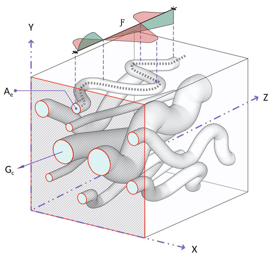
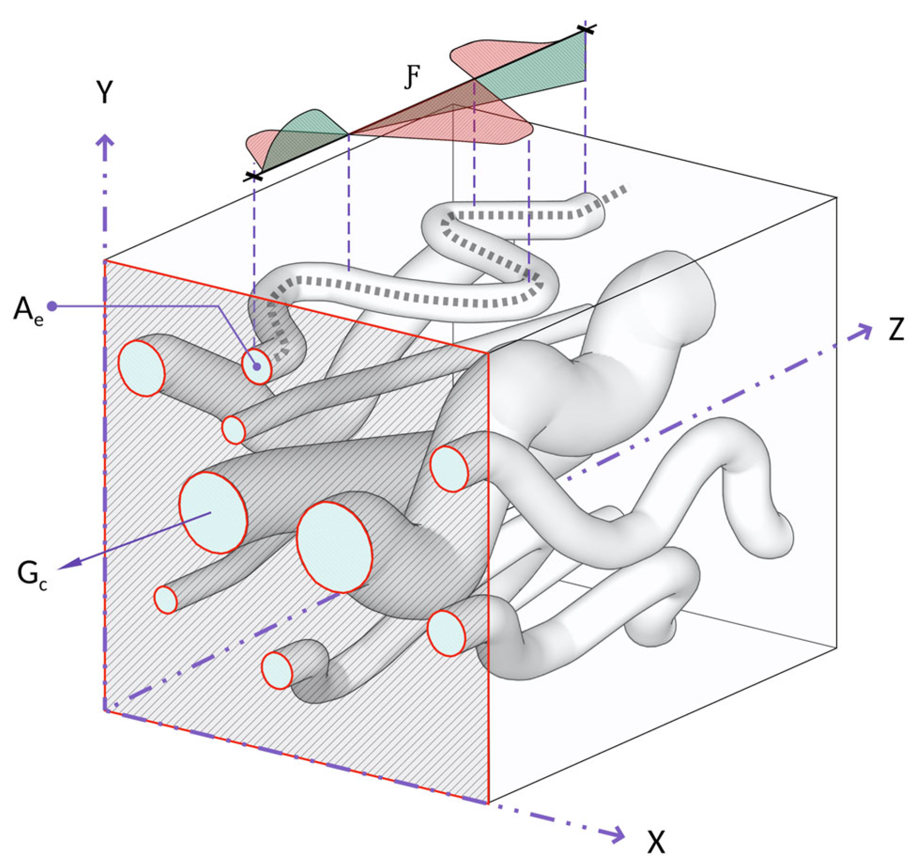
where $\mathrm{k}$ is the intrinsic permeability, $\Phi$ is the porosity, and $A_e$ is the volume-equivalent effective pore area, or effective pore throat area (on a single pore-scale).$\mathrm{Ƒ}$ is a newly introduced flowability coefficient, which represents the squared ratio of the effective transport path length to the total path length of the porous medium; it ranges between 0 and 1 and describes the geometric efficiency of the transport paths. $G$ is Glover’s [22] electrical connectedness, and $C$ is a constant that equals 8π as long as the assumptions of the model stand. These expressions describe permeability explicitly as a function of pore-geometry (Equation (3)) and electrical connectedness (Equation (4)). By combining the hydraulic and electrical formulations under a shared set of pore-scale parameters, they provide a more complete characterisation of permeability, resolving geometric features that are not captured by models that are based solely on electrical transport. Figure 1 illustrates the key parameters of the analytical model as expressed in Equations (3) and (4).

Figure 1. Schematic representation of the capillary bundle model used to conceptualise porous media, comprising fully interconnected capillaries. The X-Y cross-sectional panel highlights the effective pore throat area ${(\mathrm{A}}_{\mathrm{e}})$, which governs fluid and electrical flow through the medium. The flowability coefficient $\left(\mathrm{Ƒ}\right)$ captures both vertical and lateral convolutions along the capillary paths. Hydraulic connectedness ${(\mathrm{G}}_{\mathrm{c}})$ is an extended term of Glover’s [22] electrical connectedness ($\mathrm{G})$, which measures the availability of the pathways shared by both electrical and fluid flow.

2.1. Refinement of the New Model

The capillary bundle concept treats irregular pore spaces inside porous media as an ideal bundle of hydraulically connected tubes, where all capillaries contribute to hydraulic and electrical conduction equally. In practice, however, this is not accurate, since hydraulic conduction indeed requires hydraulic connectivity, but electrical conduction does not. Moreover, the concept’s assumptions break down in natural porous media, where both hydraulically connected and disconnected flow paths exist depending on the compositional properties and microstructural arrangement. This distinction becomes particularly clear when comparing sandy and clayey materials. Although clays often exhibit higher total porosity than sands (i.e., more capillary paths), their hydraulic conductivity is drastically lower. The underlying reason lies in the difference between total porosity $\left(\Phi \right)$ and effective porosity ${(\Phi }_e)$, where $\Phi$ represents the fraction of total capillary paths and ${\Phi }_e$ represents the fraction of only the hydraulically connected ones. In clays, $\Phi$ is substantially greater than ${\Phi }_e$, whereas in sands, they are nearly equivalent.

Therefore, to extend the applicability of the model to realistic subsurface conditions, a necessary reformation is introduced to resolve the idealised assumptions of the underlying capillary bundle concept. We divided electrical current flow into two mechanisms: first, conduction through hydraulically connected capillaries, and second, conduction through disconnected capillaries. Accordingly, we extended Glover’s [22] electrical connectedness ($G)$ to hydraulic connectedness ($G_c)$, and non-hydraulic connectedness ($G_d)$:

$$G = G_c+G_{d }$$

(5)

where $G_c={{\Phi }_e}^m$ and $G_d={{\Phi }_d}^m$. Moreover, innately, $\Phi ={\Phi }_d+{\Phi }_e$, where ${\Phi }_d$ is the disconnected (non-hydraulic) porosity and the exponent $m$ is Archie’s [1] cementation factor. The electrical conductivity of porous media ${(\mathsf{\sigma }}_t)$ is expressed by Waxman and Smits [4] as:

$${\mathsf{\sigma }}_t={\Phi }^m({\mathsf{\sigma }}_s +{\mathsf{\sigma }}_f)$$

(6)

where ${\mathsf{\sigma }}_s$ is the intrinsic electrical conductivity of the solid matrix and ${\mathsf{\sigma }}_f$ is the intrinsic electrical conductivity of the pore fluid. Applying Equation (5) to (6) yields:

$${\mathsf{\sigma }}_t={G_c{\mathsf{\sigma }}_f+G}_c{\mathsf{\sigma }}_s+G_d{\mathsf{\sigma }}_{f }{+{ G}_d\mathsf{\sigma }}_s$$

(7)

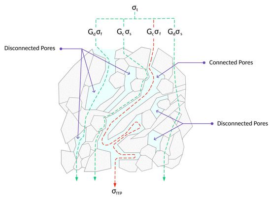
This equation can be viewed as a revised multi-path form of Waxman Smits’s model, where $G_c{\mathsf{\sigma }}_f$ is the fluid-induced conductivity at the interconnected pores, $G_c{\mathsf{\sigma }}_s$ is the solid-induced conductivity at the interconnected pore, $G_d{\mathsf{\sigma }}_f$ is the fluid-induced conductivity at the disconnected pores, and ${G_d\mathsf{\sigma }}_s$ is the solid-induced conductivity at the disconnected pores. The derivation shows that the electrical response of a porous medium comprises four distinct transport pathways, of which only one follows the same trajectories as fluid flow. Identifying the mutual pathway and isolating it from the others provides a physically consistent understanding of the shared properties between electrical conductivity and permeability and replaces existing empirical calibrations. Figure 2 illustrates the mechanics of this model. The total conductivity ${(\mathsf{\sigma }}_t)$ arises from contributions through both connected and disconnected pores, via the pore fluid ($G_c{\mathsf{\sigma }}_f$, $G_d{\mathsf{\sigma }}_{f }$) and solid matrix ($G_c{\mathsf{\sigma }}_s$, $G_d{\mathsf{\sigma }}_s$). From Equation (7), it is observed that the total electrical conductivity is induced through four distinct paths, while the fluid flow is induced through only one path. Therefore,

$${\mathsf{\sigma }}_{ffp}=G_c{\mathsf{\sigma }}_f$$

(8)

where ${\mathsf{\sigma }}_{ffp}$ is the electrical conductivity that is induced by the fluid flow alone, which represents the only shared path for hydraulic and electrical transport mechanisms. This finding addresses the limitation, better known as non-uniqueness, that occurs when attempting to infer permeability from electrical measurements. Now, rewriting Equations (3) and (4) with this consideration yields the final closed-form expressions of the new analytical model expressed by:

$$\mathrm{Pore-geometry} \mathrm{form}: \mathrm{k}= {\displaystyle \frac{1}{C }}{\Phi }_e A_e \mathrm{Ƒ}$$

(9)

$$\mathrm{Electrical} \mathrm{form}: \mathrm{k}={\displaystyle \frac{Gc{A}_e}{C}}$$

(10)

Figure 2. Pore-scale schematic of electrical conductivity pathways in fully saturated shaley sand, illustrating the four conduction mechanisms of Equation (7). The red dashed line indicates electrical conductivity along the fluid flow path, where the coupling between hydraulic and electrical transport mechanisms occurs.

2.2. Testing Data

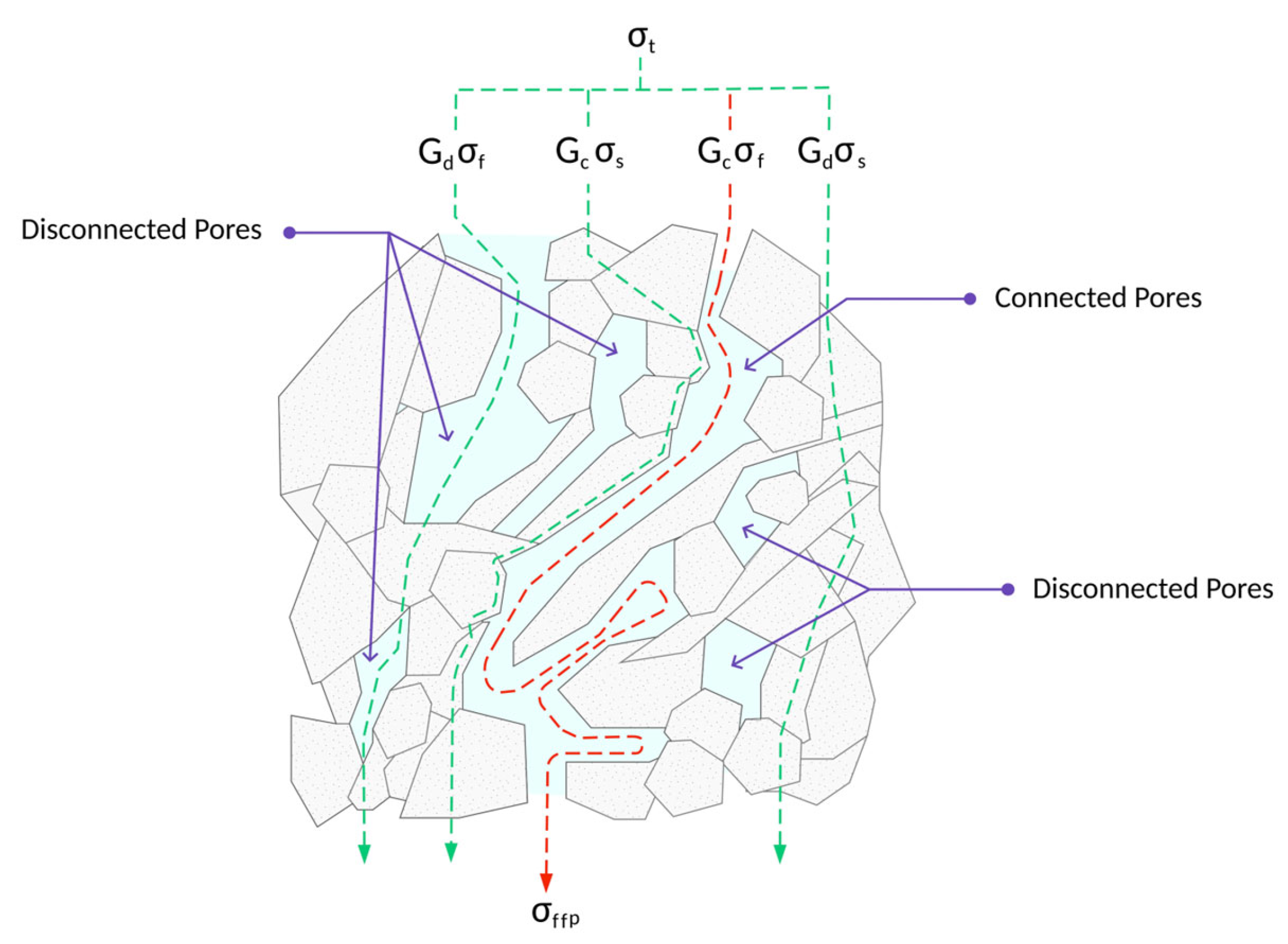
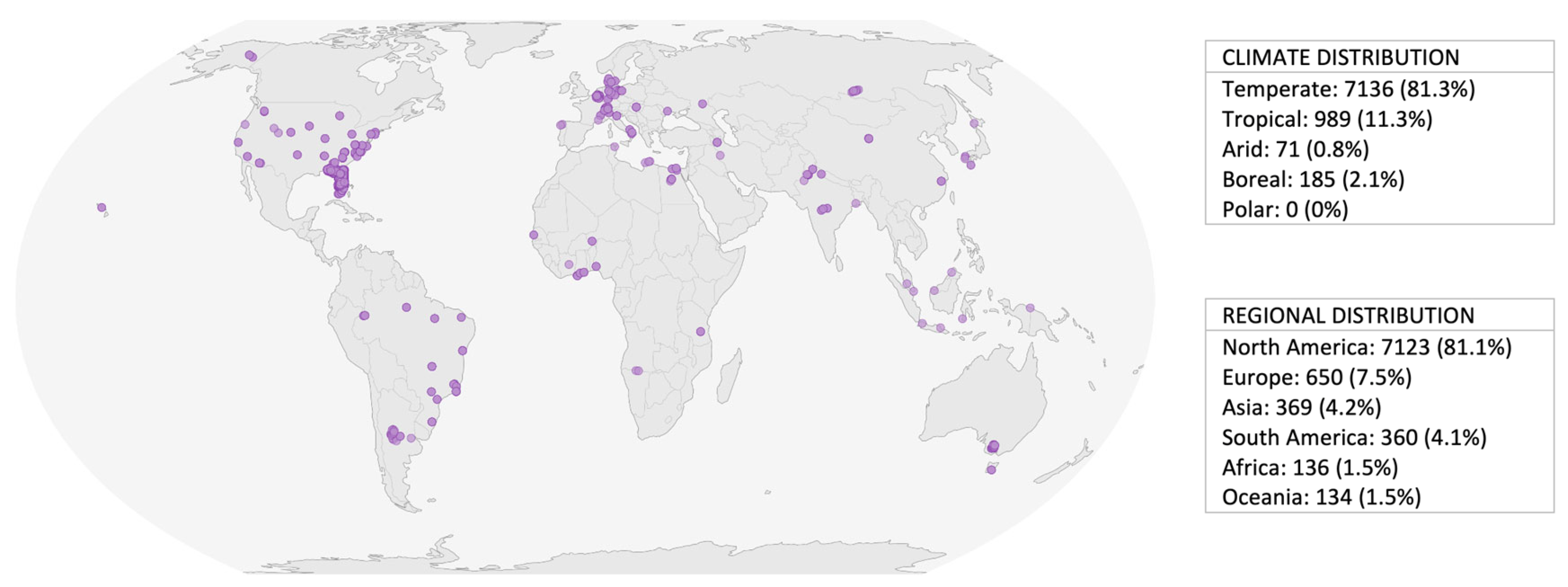
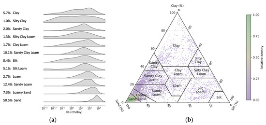
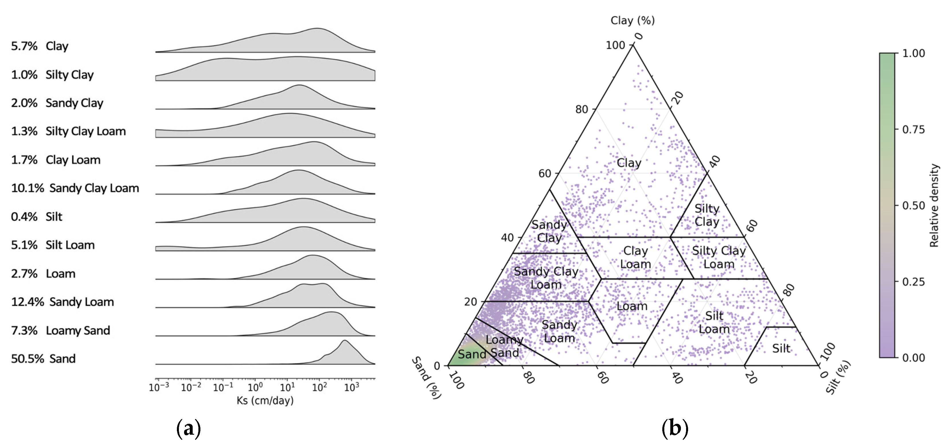
Assessments are conducted using a globally curated dataset comprising 8782 laboratory-measured permeability records from more than 1900 locations worldwide; see Figure 3. The dataset spans the entire spectrum of unconsolidated soil textures, thereby capturing the full range of hydraulic conductivity values; see Figure 4. Only laboratory measurements were retained; field-derived permeability estimates were excluded to avoid scale-mismatch effects and inconsistencies [23].

Figure 3. Global distribution of the curated data samples, including climate (Köppen–Geiger classification) and continental regional breakdowns. The dataset is predominantly concentrated in North America and the temperate climate zone.

Figure 4. Soil hydraulic characteristics of the curated dataset. (a) Distribution of saturated hydraulic conductivity (Ks) across USDA textural classes; percentages indicate each class’s share of the total dataset. (b) USDA Soil Texture Triangle, coloured by local point density.

Pore-geometry measurements including $A_e$ were not available for the samples. Therefore, $A_e$ was estimated from measured soil properties. Water flow in soils takes place in two pore domains, a capillary matrix and structural macropores [24]; thus, a dual-domain approach was used. In the capillary flow domain, the pores draining between saturation and field capacity, whose volume is the effective porosity $\left({\Phi }_e\right)$, were described by the retention equations of Saxton and Rawls [25] and converted to capillary radii with the Young–Laplace equation [26]. Their contribution to flow was expressed as a capillary flow area $\left(A_f\right)$, adapted from the capillary-bundle model of Peters et al. [26]

$$A_f=\pi {\left(2t_s\right)}^2·2{\int }_0^1{\displaystyle \frac{s}{{\left[\max \left(\psi \left(s\right),{\psi }_c\right)\right]}^2}}\mathrm{d}s$$

(11)

where $s$ is the relative position within the drainable pore range (0 at saturation, 1 at field capacity); $\psi \left(s\right)$ is the corresponding tension; $\psi c \mathrm{i}\mathrm{s}$ the tension of the largest capillary pore, set by a maximum capillary pore diameter of 0.5 mm [27,28]; and $t_s$ is the surface tension of water. In the structural flow domain, macropores carry a larger share of the flow in fine-textured soils [29]. Their contribution was represented by a multiplicative factor $\left(F_s\right)$ that depends on soil texture [30], drainable porosity [29], and bulk density $\left({\rho }_b\right)$ [31]:

$$A_e=F_s{A}_f$$

(12)

The coefficients of F_s were obtained by ordinary least squares against the required $A_e$, using 10-fold cross-validation. Reported performance was evaluated on out-of-fold (i.e., held-out) samples. The curated dataset and full reproduction scripts are provided in the dataset repository: https://doi.org/10.5281/zenodo.23327946. Of the 8782 samples, 7238 had a measured volumetric water content at 33 kPa $\left({\theta }_{33}\right)$. Following Ahuja et al. [32], samples were considered valid when ${\Phi }_e\ge 0.04$ and $0 < {\theta }_{1500} < {\theta }_{33}$, which excluded 553 samples. Samples outside the original calibration domain of the retention equations [25] $({\rho }_b< 1.0 \mathrm{or} > 1.8 \mathrm{g} {\mathrm{c}\mathrm{m}}^{-3}$; organic matter $> 8\%$ or clay $> 60\%)$ were also excluded (291 samples). Finally, outliers in log-permeability within each texture class were removed with a threshold of three median absolute deviations, a very conservative criterion [33], which removed 106 samples, resulting in a total of 6288 physically consistent samples, which were used for the evaluations in this manuscript.

2.3. Global Convergence and Comparative Analysis

Model performance was benchmarked against two distinct tiers of existing approaches. First, against seven of the most widely established PTFs, including Cosby et al. [34], Saxton et al. [35], Brakensiek et al. [36], Ferrer-Julià et al. [37], Puckett et al. [38], Dane and Puckett [39], and Campbell and Shiozawa [40]. Second, against established and widely used theory-based permeability analytical and semi-empirical models, namely, Kozeny–Carman [3], Johnson–Koplik–Schwartz (JKS) [8], and Revil and Cathles [12]. The evaluation framework adopted in this study deliberately provided a rigorous assessment of predictive capability by benchmarking models on a globally diverse dataset without calibration.

Predictions were assessed using the coefficient of determination (R²), root mean square error (RMSE), mean absolute error (MAE), median error (MdE), and mean error (ME), following standard regression diagnostics [41]; the Pearson correlation coefficient (r) [42]; the Spearman’s rank correlation coefficient $\left(\rho \right)$ [43]; the Nash–Sutcliffe efficiency (NSE); and the Kling–Gupta efficiency (KGE) [44].

2.4. Stress Testing and Uncertainty Propagation

Uncertainty handling was evaluated using Monte Carlo simulation, an approach recommended for nonlinear models [45]. The input parameters $G_c$ and $A_e$ of the model (Equation (10)) were perturbed simultaneously in every realisation. The relative uncertainty level was increased from ±5% to ±200% in steps of 5% (40 levels), with 120 realisations per level, each perturbing all 6288 samples. Permeability was recomputed from the perturbed inputs and compared with the measured values in log₁₀ space.

Since $A_e$ is strictly positive and spans several orders of magnitude, its error was modelled as a multiplicative lognormal factor. For a prescribed level, taken as the coefficient of variation (CV) of the factor, the log-scale standard deviation is $\sigma = \surd ln(1 + C{V}^2)$. The factor is median-preserving, $e^{\sigma z}$ with $z ~ N\left(\mathrm{0,1}\right)$; so, perturbations retain the right-skewed nature of original data. $G_c$ is physically bounded by 0 to 1. Its error was applied in logit space, which keeps $G_c$ within the physical range by design. The logit-space scale was calibrated by bisection so that the achieved CV of the perturbation matched the prescribed level. The two inputs therefore share the same nominal uncertainty level, but it is expressed on the scale appropriate to each variable. Moreover, $A_e$ and $G_c$ are not independent in the data (Spearman $\rho = 0.81$); to reproduce that, we used Iman & Conover rank-correlation procedure [46], which imposes the target rank correlation $\left(\rho \right)$ without bypassing the physical conditions discussed earlier. The target $\rho$ was held fixed across all uncertainty levels. Uncertainty values of $A_e$ and $G_c$ are not intended to represent realistic experimental error at every level. The lower levels (<100%) are intended to evaluate the model across degraded data quality scenarios. The upper levels deliberately exceed plausible error and are aimed at locating the level of input uncertainty at which predictive skill fails.

3. Results

3.1. Dimensional Consistency and Asymptotic Behaviour

As presented in Equation (9), dimensional consistency was examined using the Buckingham Pi theorem [47], whereby permeability is normalised by the effective pore area as ${\pi }_1 = k/A_v$, and the unitless parameters remain as ${\pi }_2=\mathrm{Ƒ}$ and ${\pi }_3={\Phi }_e$. Thus, the analytical model reduces to a compact dimensionless scaling law: ${\pi }_1 = {\pi }_2 {\pi }_3/c$. This form shows no deviation in behaviour compared to the original dimensional form. Thus, the governing length scale has been correctly identified, and no hidden dimensional dependencies exist.

The asymptotic behaviour of the model was examined at physically meaningful limits, following standard practice in porous-media theory [6]. When porosity approaches zero, permeability approaches zero $\left(\Phi \to 0; \mathrm{k}\to 0\right),$ since loss in void space leads to loss in the porous potential of a medium. However, porosity approaching the unity, which signifies a single connected pore, leads to permeability becoming a function of effective pore area and flowability, $\Phi \to 1; \mathrm{k}(A_e,\mathrm{Ƒ}).$ This is consistent with Bear’s [5] definition of permeability in a single straight cylindrical pore. The flowability coefficient, $\mathrm{Ƒ}$, describes the efficiency of the connected transport paths; $\mathrm{Ƒ}\to 1$ represents a perfectly straight path, while $\mathrm{Ƒ}\to 0$ represents an infinitely convoluted path. Thus, if the path is straight, permeability becomes a function of effective pore area, $\Phi \to 1, \mathrm{Ƒ}\to 1; \mathrm{k}\left(A_e\right)$. If $\mathrm{Ƒ}\to 0$, signifying a path where tortuosity $\left(\mathsf{\tau }\right)$ is approaching infinity $(\mathsf{\tau }\to {\mathrm{\infty }}^2)$, since $\mathrm{Ƒ}={\displaystyle \frac{1}{{\mathsf{\tau }}^2}}$, permeability and effective pore area approach zero ($A_e\to 0) \mathrm{and} (\mathrm{k}\to 0)$, despite the value of porosity. This case can be seen in the behaviour of clayey soils. $A_e\to 0$ represents a loss of transmissive capacity of connected paths. Thus, we can conclude that $A_e$ and $\mathrm{Ƒ}$ are interrelated; $A_e\to 0 \mathrm{r}\mathrm{e}\mathrm{s}\mathrm{u}\mathrm{l}\mathrm{t}\mathrm{s} \mathrm{i}\mathrm{n} \mathrm{Ƒ}\to 0; \mathrm{k}\to 0. \mathrm{A}\mathrm{n}\mathrm{d} \mathrm{Ƒ}\to 0 \mathrm{r}\mathrm{e}\mathrm{s}\mathrm{u}\mathrm{l}\mathrm{t}\mathrm{s} \mathrm{i}\mathrm{n} A_e\to 0$; $\mathrm{k}\to 0$. The absence of non-physical asymptotes confirms that the formulation is valid across the admissible parameter space and consistent with continuum flow theory [48].

3.2. Global Convergence and Comparative Analysis: Results

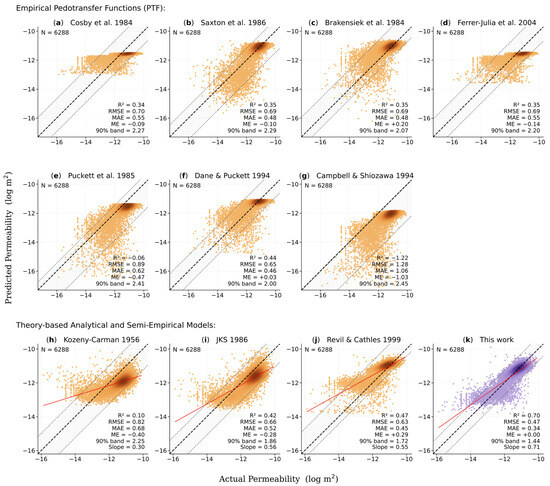
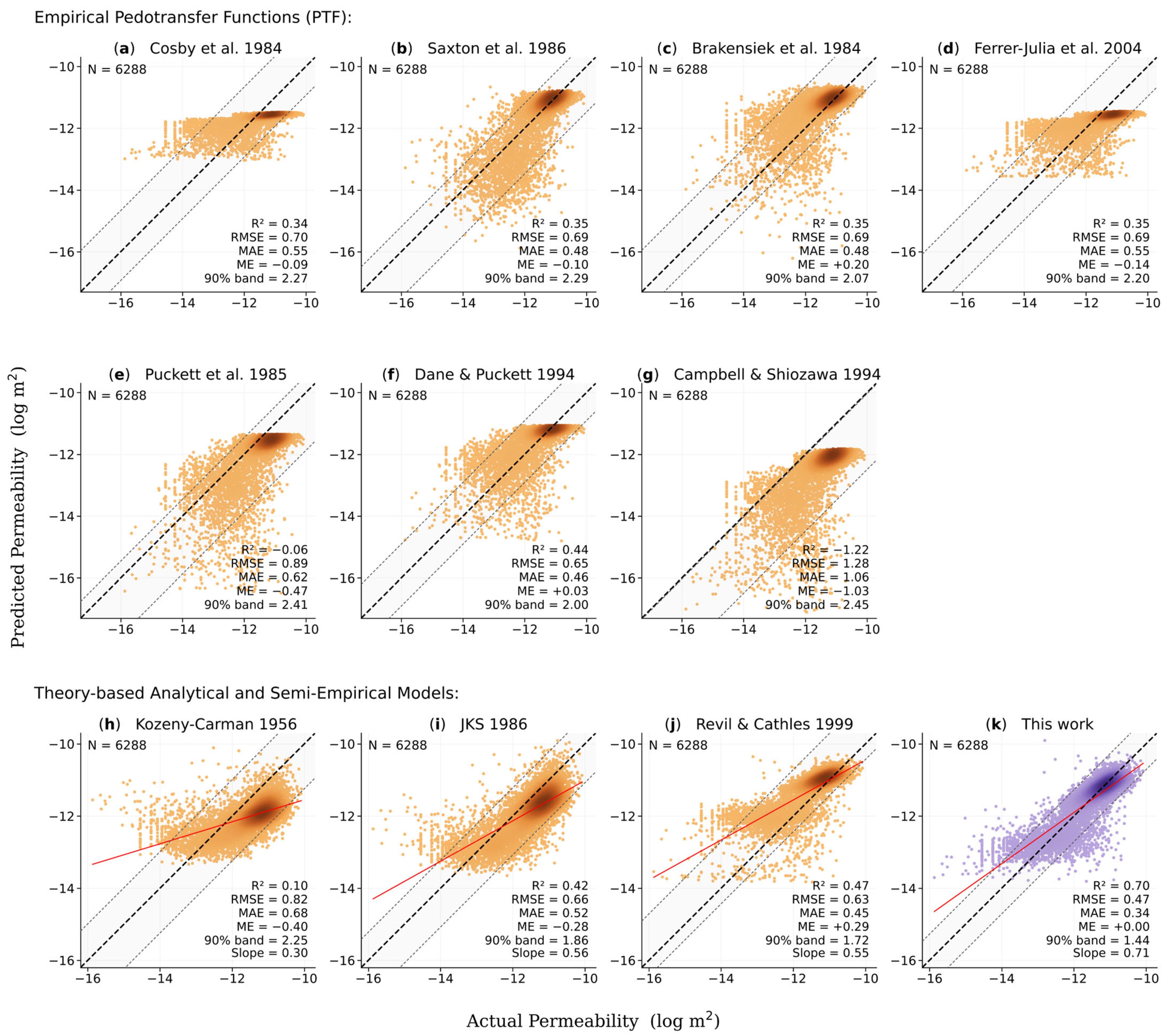
Model performance is benchmarked against two distinct tiers of existing approaches. First, against the most widely used empirical pedotransfer functions (PTFs); and second, against the established analytical and semi-empirical permeability models. Figure 5 shows the global performance comparison between this work and two model tiers. Model performances are discussed in the following paragraphs.

Figure 5. Global performance comparison between this work and two model tiers: empirical pedotransfer functions (upper) and theory-based analytical and semi-empirical models (lower). The empirical tier comprises seven established PTFs (Cosby et al. [34]; Saxton et al. [35]; Brakensiek et al. [36]; Ferrer-Julià et al. [37]; Puckett et al. [38]; Dane and Puckett, [39]; Campbell and Shiozawa, [40]). The theory-based tier comprises the Kozeny–Carman formulation [3], the Johnson–Koplik–Schwartz model [8], and Revil and Cathles model [12]. All models are evaluated on the same 6288 samples. Point shading denotes sample density, grey shading indicates the 90% band range, and the dashed line is the 1:1 relation. This work demonstrates the highest predictive power (R² = 0.70) and the lowest error (RMSE = 0.47; MAE = 0.34).

The performance scatter plots (Figure 5) show arbitrary deviations across all permeability ranges with comparable compression (see Figure 5a,d) and expansion (see Figure 5b,c,e–g) patterns, with a clear upper prediction cap. These scatter patterns, along with the low convergence metrics (R² = 0.34 to 0.44), suggest a poor global performance. Figure 5e,g show negative convergence and high bias and, thus, are excluded from the discussion. The PTFs showed markedly similar median error metrics, i.e., RMSE ≈ 0.70 log m² and MAE ≈ 0.50 log m². The grey shaded zone illustrates the 90% band, where measurements on average exceed two orders of magnitude across all PTFs.

These findings suggest that using readily available soil properties, e.g., soil texture and bulk density, do not fully capture permeability. This does not invalidate PTF use with proper calibration but rather emphasises the challenges of developing universally applicable hydraulic property estimators using purely empirical approaches.

As illustrated in the lower panels of Figure 5, theory-based formulations exhibit a clear improvement in global data scatter relative to the empirical PTFs above. Prediction residuals evolve from high-variance distributions (see Figure 5a–g) to more systematically structured patterns with reduced dispersion and near-parallel alignment with the 1:1 reference line (see Figure 5h–j). Notably, despite being derived from distinct theoretical backgrounds, the theory-based models display broadly similar predictive behaviour, implying consistent underlying physical constraints governing permeability estimation. Their global convergence metrics and median error metrics are similar to the results of the PTFs, except their systematic scatter patterns make theory-based models the superior contender.

The Kozeny–Carman model, as expressed in Equation (13), is widely regarded as the industry standard and represents the most frequently cited permeability relationship in the literature.

$$k={\displaystyle \frac{d^2}{36C_k}}{\displaystyle \frac{{\mathsf{\varphi }}^3}{{(1-\mathsf{\varphi })}^2}}$$

(13)

The mean grain diameter $\left(d\right)$ in our application was taken as $d = 2{\mathrm{R}}_e$ where ${\mathrm{R}}_e$ is the effective radius of the flow path as suggested by Revil and Cathles [12]. Considering an effective pore area $A_e$ of a quasi-circular shape, ${\mathrm{R}}_e$ can thus be computed. This parameter enhances the Kozeny–Carman equation to function at a broader range rather than being restricted to sands alone, as ${\mathrm{R}}_e$ accounts for the effects of the electrical double layer (EDL) [49,50], which the Kozeny–Carman equation is otherwise blind to. That said, it seems reasonable to assume that its performance is still severely restricted ($R^2=0.10, ME=- 0.40, RMSE=0.82 \log {\mathrm{m}}^2$) due to the dependence on total porosity $\left(\Phi \right)$ and the empirical constant ${(C}_k)$. The use of $\Phi$ does not allow the distinction between hydraulically and non-hydraulically connected pores as ${\Phi }_e$ does (see Section 2.1); as a result, it approximates the available flowpaths based on $d$. Furthermore, $C_k$ is theoretically defined by the shape and tortuosity of flow paths. However, because measuring these geometries in situ is highly impractical, it is widely accepted as 5 for granular media [6,51,52].

The JKS [8] is an analytical model that is based on a characteristic length scale $\left(\Lambda \right)$, which explicitly captures the EDL effects and the deviations from idealised bulk-fluid electrical behaviour. The model links pore-scale characteristics and electrochemical interactions:

$$k={\displaystyle \frac{{\Lambda }^2}{2F}}$$

(14)

Λ is defined as a length scale and represents a weighted analogue of the length $2V_p/S$ [49], where $V_p$ is the interconnected pore volume and $S$ is the pore surface area. $\Lambda$ was defined originally as:

$${\displaystyle \frac{2}{\Lambda }}={\displaystyle \frac{{\int }_S{\left|e_b\right|}^{2}dS}{{\int }_S{\left|e_b\right|}^{2}d{V}_p}}$$

(15)

where ${\mathrm{e}}_{\mathrm{b}}$ is the normalised electrical field in the interconnected pore space. Since $\Lambda$ is a parameter that is difficult to determine, [12] redefined $\Lambda$ as:

$$\Lambda ={\displaystyle \frac{{\mathrm{R}}_e}{m(F-1) }}$$

(16)

We used this definition of $\Lambda$ in the evaluation of the model. We found that $\Lambda$ increases proportionally but not monotonically with grain size and ranges from 10⁻⁴ for coarse-grained soils to 10⁻¹¹ for fine-grained soils. As seen in Figure 5i, while the JKS performance is modest $(R^2 = 0.42, ME = - 0.28, RMSE = 0.82 \mathrm{l}\mathrm{o}\mathrm{g} {\mathrm{m}}^2)$, it seems to be capped by an underestimation tendency. This is likely due to the result from an overly conservative treatment of EDL effects that exaggerates their hindering influence on permeability. On the other hand, this may also be attributable to estimating $\Lambda$ indirectly using Equation (16), rather than through direct lab measurement as specified in Equation (15). Both Kozeny–Carman and JKS models display a necessity for site-specific calibration to achieve reliable permeability estimates.

Revil and Cathles [12] proposed a permeability expression derived from the theoretical frameworks of Carman [3], Johnson et al. [8], Kostek et al. [53], Marion et al. [54], and Bernabé [11]. The model incorporates three conditional power-law corrections designed to extend the applicability of permeability predictions to shale-bearing media as follows:

$$k_{sd}={\displaystyle \frac{{d^2{\mathsf{\varphi }}_{sd}}^{3m_{sd}}}{24}}$$

(17)

$$k_{sh}=k_{sd}{\left({\mathsf{\varphi }}_{sh}\right)}^{{3m}_{cs}} f_c={\mathsf{\varphi }}_{sd}$$

(18)

$$k_{sh}=k_{sd}{\left(1-{\mathrm{f}}_c\left({\displaystyle \frac{1-{\mathsf{\varphi }}_{sh}}{{\mathsf{\varphi }}_{sd}}}\right)\right)}^{3m_{cs}} f_c<{\mathsf{\varphi }}_{sd}$$

(19)

$$k=k_{sh}{\left({\mathrm{f}}_c\right)}^{m_{sd}} f_c>{\mathsf{\varphi }}_{sd}$$

(20)

where $k_{sd}$ is the permeability of clean sand or sandstone, measured with the porosity of sand, ${\mathsf{\varphi }}_{sd}$, and the cementation exponent of sand, ${\mathrm{m}}_{sd}$, which we found to be 1.44 ± 0.123 across our data, depending on amount of impurities in sand (e.g., fine minerals, carbon content). The shale end-member permeability $k_{sd}$ is related to the shale end-member porosity ${\mathsf{\varphi }}_{sh}$. ${\mathrm{f}}_c$ is the clay volume fraction, and $m_{cs}$ is the cementation exponent corresponding to the clayey sand domain, ranging from 1.50 to 2.38, driven primarily by the soil composition. The model presented by Revil and Cathles [12] demonstrated a modest predictive accuracy ($ME = +0.29, RMSE=0.63 \mathrm{l}\mathrm{o}\mathrm{g} {\mathrm{m}}^2$; see Figure 5j), driven primarily by its over-estimation tendency. While this model utilises clay volume like some PTFs to infer permeability, its theoretical foundation enables a broader model transferability ($R^2=0.47$; 90% band within 1.72 orders of magnitude).

The model presented by this work, as shown in Figure 5k, demonstrates noticeably superior performance compared to other models, evident by the highest global convergence $(R^2= 0.70)$ and the highest predictive accuracy ($RMSE=0.47, MAE = 0.34 \mathrm{l}\mathrm{o}\mathrm{g} {\mathrm{m}}^2$, 90% band within 1.44 orders of magnitude). This signifies a major advancement over existing models and emphasises the value of explicitly integrating pore-scale physics to predict permeability, as formulated in Equations (9) and (10).

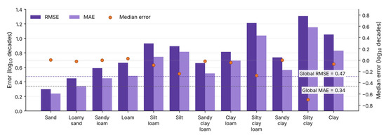
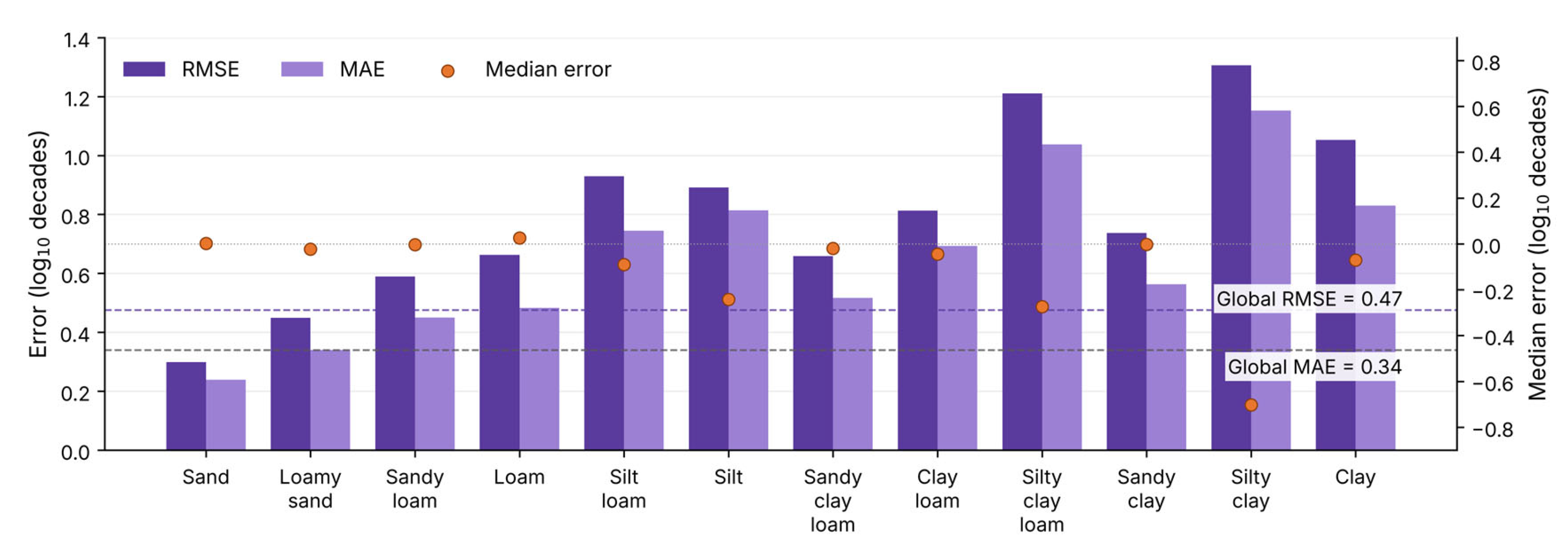
Model errors rise from coarse to fine textures (see Figure 6), with RMSE increases from $0.30 \log {\mathrm{m}}^2$ in sand to $1.05 \mathrm{l}\mathrm{o}\mathrm{g} {\mathrm{m}}^2$ in clay, following a gradient that is broadly systematic but not strictly monotonic; silty clay loam, at $1.21$, already exceeds several finer classes, and silty clay, at $1.31$, exceeds clay. Otherwise, the structure closely follows the data pattern: within-class RMSE correlates strongly with the intrinsic dispersion of permeability $(r = 0.81)$, rising with clay fraction $(r = 0.79)$ and falling with sand fraction $(r=-0.83)$, all significant at $p < 0.01$. Fine-textured soils simply span a far wider range of permeability, with the standard deviation of permeability rising from $0.27 \log {\mathrm{m}}^2$ in sand to $0.73 \log {\mathrm{m}}^2$ in clay; absolute error grows with texture even where the model continues to resolve most of the within-class variance. The nature of this error confirms a dispersive rather than methodical regime, with mean error confined to $\pm 0.01$ log ${\mathrm{m}}^2$ across all twelve soil classes and showing no dependence on texture, locating the residual error in the natural heterogeneity of fine-textured media rather than in the model formulation; this is confirmed by the median error, as it declines where the behaviour in a certain class is inconsistent.

Figure 6. Global er-texture-class error of the analytical model (this work) across the twelve USDA soil textures, ordered from coarse to fine. Bars show RMSE (dark purple) and MAE (light purple) on the left axis; orange markers show median error (MdE) on the right axis. Dashed lines denote global values (RMSE = 0.47, MAE = 0.34, ME < 0.01); all errors are in log decades.

3.3. Stress Testing and Uncertainty Propagation: Results

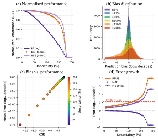
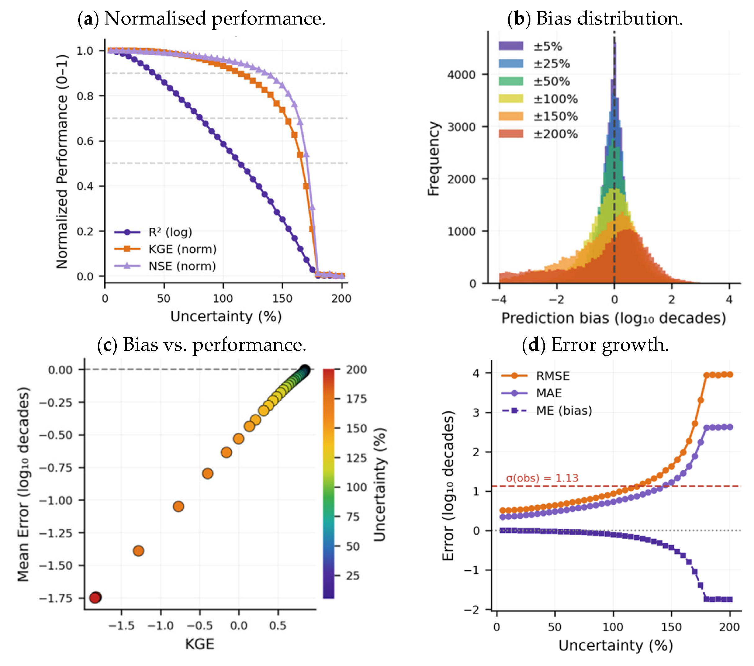
Uncertainty handling was evaluated using Monte Carlo simulation, an approach recommended for nonlinear models [45]. Uncertainty perturbations are applied independently to input parameters, starting with an initial value of ±5% and increasing to a terminal value of ±200% of each parameter’s variance $\mathcal{N}\left(1,{\sigma }^2\right)$. Figure 7 shows the Monte Carlo simulation demonstrating the model’s performance thresholds under increasing parametric uncertainty.

Figure 7. Model’s performance thresholds under increasing parametric uncertainty using Monte Carlo simulation on 6288 test samples. (a) Normalised performance, (b) bias distribution, (c) bias versus performance, and (d) error growth.

Under Monte Carlo perturbation, the model degrades progressively from a baseline of R² = 0.70; skill is retained above R² = 0.65 to 31% uncertainty and above R² = 0.60 to 47% (Figure 7a). NSE falls below 0.5 at 79% and reaches zero at 120%, whereas KGE crosses zero only at 155%. Since NSE penalises variance inflation while R² responds only to correlation, this ordering identifies dispersion as the failure mechanism. The KGE decomposition correlation term is retained the longest, and the variability ratio inflates first (see Figure 7c); so, the model continues to rank permeability correctly after absolute magnitudes become unreliable. Mean error stays within 0.11 log units to ±100%, and bias distributions remain centred while broadening symmetrically, as shown in Figure 7b, indicating that input error propagates as variance rather than systematic drift. According to Figure 7d, errors grow gently to about ±150% and then accelerate. The red line (σ = 1.13) is where prediction error equals the natural spread of the data (i.e., model failure); RMSE crosses the red line only at ±119% and MAE at ±146%, indicating a markedly high tolerance to data uncertainty.

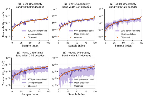
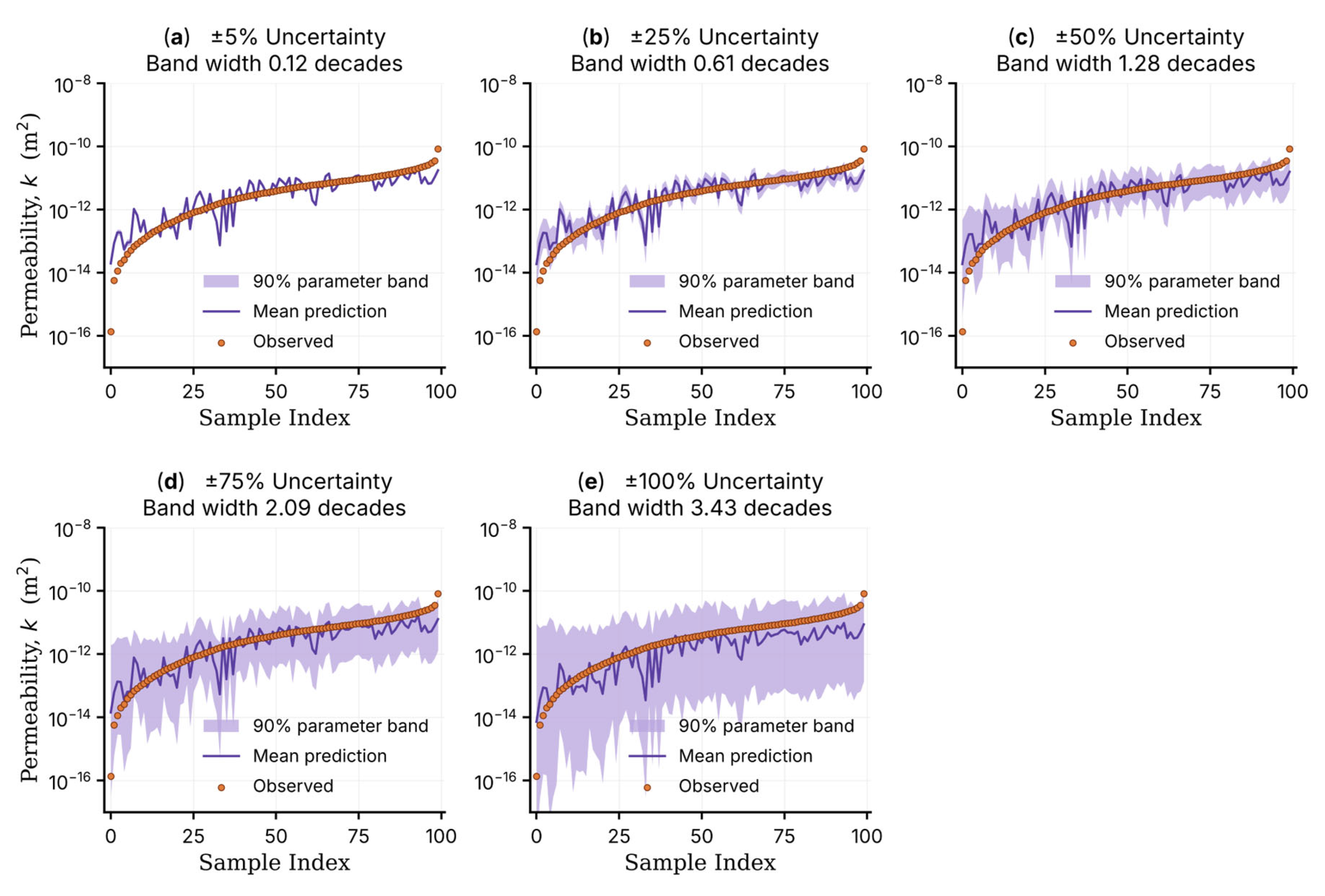
Parameter propagation (Figure 8) widens the predictive band from 0.12 log units (decades) at ±5% to 3.43 log decades at ±100%, a near-linear response confirming the absence of amplification through the analytical form [55].

Figure 8. Sensitivity of prediction uncertainty bands to imposed parametric uncertainty, illustrating progressive expansion of the confidence region with increasing parametric uncertainty from ±5% to ±100%.

The stress-testing demonstrates that the model remains highly viable under extreme data-uncertainty conditions. This indicates the model is not overly sensitive to degradation in input data quality and can provide meaningful estimates even when parameter data quality is low [56]. Such behaviour features the model’s versatile applicability in subsurface exploration, where data are often sparse, heterogeneous, and subject to measurement and interpretation errors, and where strict control over input quality is rarely achievable [57].

4. Discussions

4.1. Physical Meaning

The presented model was derived by analytically linking hydraulic and electrical properties from first principle theories (i.e., Navier Stokes and Ohm’s law) under a shared set of pore-scale parameters. The model provides a more complete characterisation of permeability, resolving geometric features that are not captured by models that are based solely on electrical transport (e.g., Archie’s law), empirical models that rely on soil covariates (i.e., PTFs), models that are based solely on simplified pore geometry proxies (e.g., Revil & Cathles, Kozeny–Carman), or analytical models that rely singularly on a length scale (e.g., JKS).

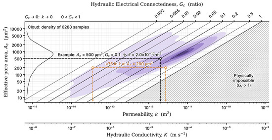
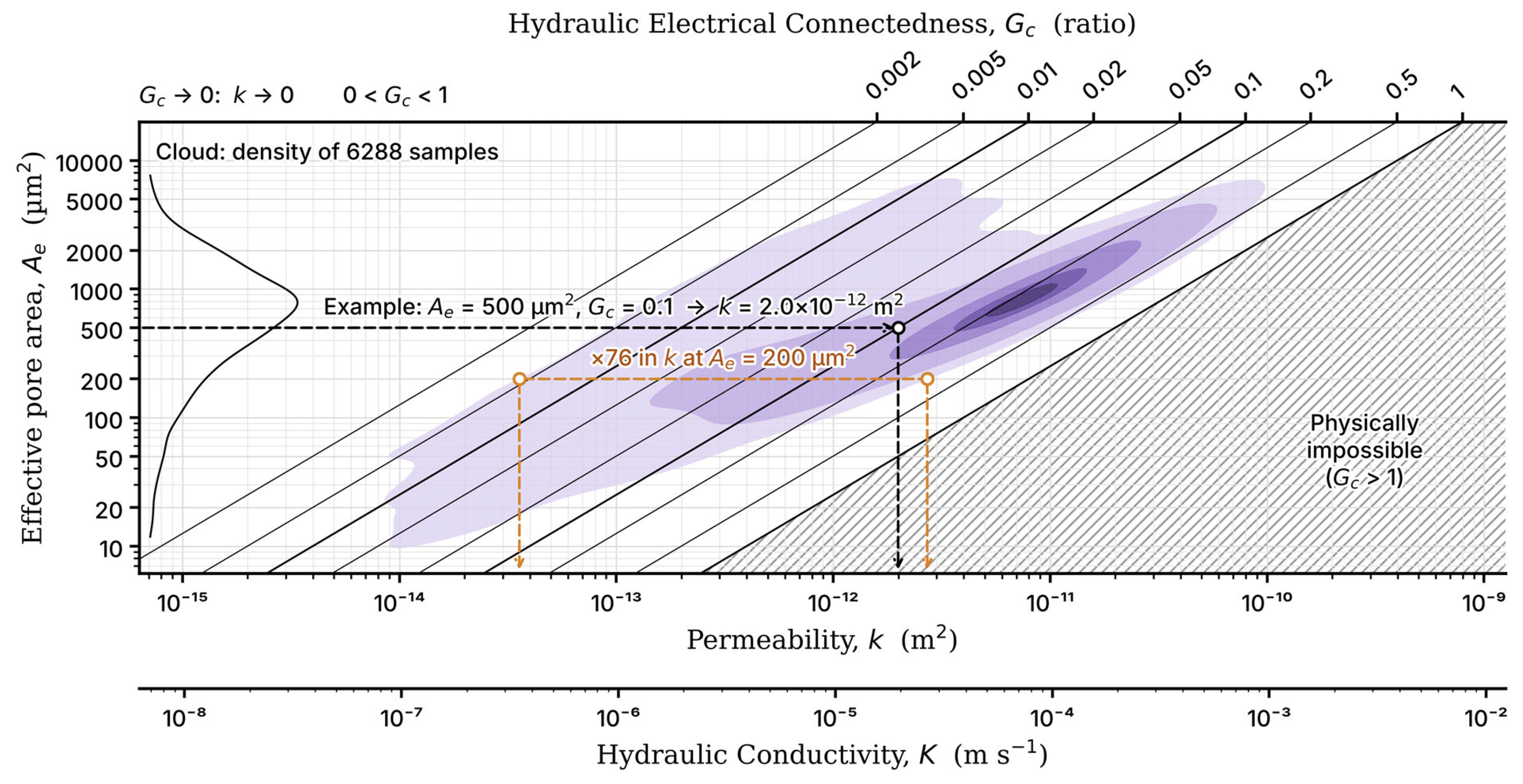
The advantage of the new model lies in the physics of permeability. We found that the relationship between $k$ and $A_e$ is multimodal: the same $A_e$ can span over 76-fold range of $k$ (Figure 9), because $A_e$ is a total measure of conductive pore space; it is blind to flow paths ratio $\left({\Phi }_e\right)$ and tortuosity. In the new model as presented by Equation (10), geometric parameters are proxied by $G_c$, which measures how permeability $\left(k\right)$ responds to changes in pore space $(\mathrm{i}.\mathrm{e}.,{ A}_e)$. Since $G_c$ predicts the efficiency of the path, a flowing fluid takes by interpreting the electrical response of that path (Equation (7), Figure 2). In Equation (9), the model substitutes the proxy parameter, $G_c$ with explicit pore-geometry expressions $({\Phi }_e$ and $\mathrm{Ƒ})$ that behave in the same manner. This explicit pore-scale characterisation of $k$ drives the model’s superior performance.

Figure 9. A graphical representation of Equation (10), where permeability $\left(k\right)$ is a function of effective pore area ${(A}_e)$ and hydraulic electrical connectedness $\left(G_c\right)$. The cloud represents 6288 samples, with kernel density shown in purple gradient, shaded at 95, 75, 50, 25, and 10% of the data. The curve on the left shows the distribution of $A_e$. $k$ for any combination of ${ A}_e$ and $G_c$ is read where the two intersect, as in the presented example. The orange line is an example of the uncertainty produced by measuring $k$ from $A_e$ alone. The lower axis shows the equivalent hydraulic conductivity $\left(k\right)$ for a pore fluid of electrical conductivity 0.2 S m⁻¹ at 20 °C.

4.2. Applicability and Limitations

The new model is derived within a continuum-physics framework incorporating electrokinetic considerations for medium-to-high salinity fluids percolating through fully saturated porous media under laminar flow conditions. It relies on classical assumptions of Hagen–Poiseuille flow, appropriate for unconsolidated soils and sediments only. It does not explicitly account for consolidated media, turbulent flow regimes, and pore-filling phases such as gas hydrates.

Permeability prediction of the presented model appears to degrade proportionally as finer particles increase in soil (see Figure 6), with the highest error seen in the clayey soils. Beyond the statistical rationale discussed earlier, the apparent degradation in performance has a physical nature. In sands, porosity and permeability are quasi-proportional [58]. However, clays depend on clay mineral type; unlike sands, clay types govern pore geometry based on their swelling capacity. Moreover, different clay types are dominant in different parts of the globe, categorised by climate type [59]. As a result, the behaviour of clayey soils is found to be inconsistent across regions and climates despite identical soil proportions [59]. Montmorillonite and illite-smectites (predominant in temperature and arid zones, respectively), due to their high swelling potential (up to ten times in volume), fill and plug pores more effectively than kaolinite (predominant in tropical regions) with low swelling potential; as a result, the latter yields markedly higher connectivity and permeability [60]. The model distinguishes between clay types based on its physical awareness of solid matrix conductivity (${\sigma }_s)$, revised in Equation 7. Where ${\sigma }_s$ is proportional to the swelling potential, it peaks in montmorillonite and smectites (~500 mS/m), decreases in illites (~200 mS/m), and troughs in kaolinites (~30 mS/m) [61]. This indicator is successful in enabling the model to be aware of clay types and their consequences; see Figure A3 in Appendix A. Thus, the model is able to function even in clayey soils. However, swelling is not a fixed property of a clay mineral but a response to its environment. The same clay type can swell very differently depending on pore-water salinity, exchangeable cation type, pH, and temperature [62]. As a result, higher ambiguity is associated with clayey soils, as seen in Figure 6.

Having addressed the effects of different climates on soil properties, we note that the curated dataset is geographically and climatically unbalanced: 81.1% of the samples originate from North America and 81.3% from temperate climates (Figure 3), and no samples come from polar regions. This imbalance may reduce the reliability of the model’s predictions outside temperate regions. However, because the model is largely analytical, the imbalance is expected to matter less than for purely empirical models. The underrepresented tropical $(11.3\%, n=989)$, arid $(5.4\%, n=471)$, and boreal $(2.1\%, n=186)$ zones together span a wide range of permeabilities $({\log }_{10}k \approx -14 \mathrm{to} -11)$, like that of the temperate zone, which suggests that the main physical gradients are represented. Nevertheless, predictions for these regions should be interpreted with caution until local validation in the underrepresented zones is conducted.

5. Conclusions

Subsurface characterisation through the integration of soil information and electrical methods has been progressively advanced by a substantial body of work, including that of Kozeny [63], Muskat [64], Jacob [65], Archie [1], Maillet [2], Carman [3], Waxman & Smits [4], Bear [5], Dullien [6], Bussian [7], Johnson et al. [8], Katz and Thompson [9], Sen, Goode & Sibbit [10], Bernabé [11], Revil & Cathles [12], Weller, Slater & Nordsiek [13], Salem [14], and Glover [15]. Each addressed a distinct aspect of the underlying theory.

In this study, two contributions are made to the field of hydrogeophysics. First, we derive, from the Navier–Stokes equations and Ohm’s law, a closed-form model that describes permeability as a function of electrical conductivity and pore geometry. Second, we explain and address the non-uniqueness of electrical conductivity as a predictor of permeability by revealing four distinct electrical transport paths in porous media, of which only one aligns mechanistically with fluid-flow trajectories. We benchmark the new model against ten widely used permeability models, including empirical and theoretical models on a broad global dataset of 6288 laboratory samples, spanning the entire soil texture spectrum from sand to clay. It achieves superior predictive accuracy $(R^2 = 0.70; RMSE = 0.47, MAE = 0.34, bias < 0.01 \mathrm{all} \mathrm{in} \log 10 {\mathrm{m}}^2)$ and remains stable across soil textures, with errors rising from sand $(RMSE = 0.30 \log {\mathrm{m}}^2)$ to clay $(RMSE = 1.05 \log {\mathrm{m}}^2)$. Monte Carlo simulations reveal robustness $(R^2 > 0.60)$ under data uncertainties of up to 47% and maintain stable error gains up to 100%. The model reaches failure at 119% of data uncertainty, indicating markedly high tolerance to data uncertainty.

We also found that pore area alone is insufficient for reliable permeability prediction, with errors spanning several orders of magnitude, as it does not account for the distribution of transport pathways or their tortuosity. The new model measures these parameters by effective porosity and the newly coined flowability coefficient (Equation (9)) or it proxies them using an expanded term, hydraulic electrical connectedness (Equation (10)).

As a result, this work provides a more complete characterisation of permeability by resolving geometric features that are not captured by models that are based solely on electrical transport (e.g., Archie’s law), empirical models that rely on soil covariates (i.e., PTFs), models that are based solely on simplified pore geometry proxies (e.g., Revil & Cathles, Kozeny–Carman), or analytical models that rely singularly on a length scale (e.g., JKS).

Appendix A.1. The Cylindrical Pore Concept

Fluid flow in a single connected pore can be visualised using a pipe model with a length $\left(L\right),$ and a radius $\left(r\right),$ under the effect of a pressure gradient $(\nabla P)$. See Figure A1.

Figure A1. The cylindrical-pore model, representing flow in a single connected pore.

Figure A1. The cylindrical-pore model, representing flow in a single connected pore.

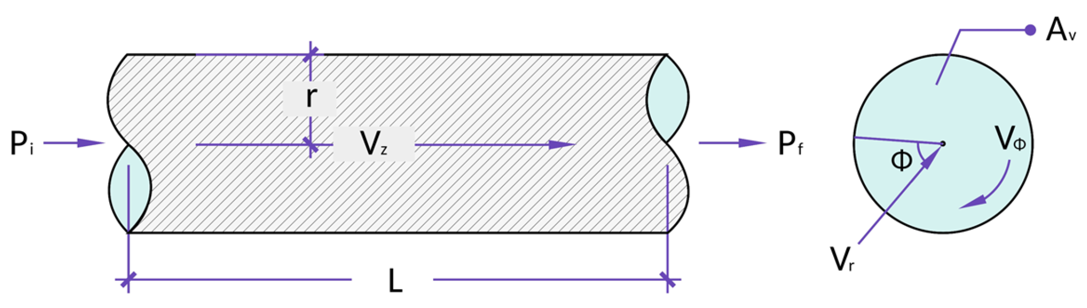
We applied the continuity and Navier–Stokes equations to a case of fluid flow in a microenvironment such as a single connected pore that is always fully saturated, where the flow is in a steady state, and gravity plays a negligible role in moderating flow. Additionally, the flow is visualised to travel in a straight path under the influence of the pressure gradient. These considerations produce the Hagen–Poiseuille’s Law [72]:

$$\mathsf{\Delta }P={\displaystyle \frac{8\mathsf{\pi }\mu LQ}{A^2}}$$

(A1)

Now, the discharge of a single cylindrical pore is expressed by:

$$Q={\displaystyle \frac{\mathsf{\Delta }P{A_v}^2}{8\mathsf{\pi }\mu L_v}}$$

(A2)

where $A$ (also denoted $A_v$) is area of the pore, L (also denoted $L_v$) is the length of a single connected pore path, $\mu$ is dynamic viscosity, $\rho$ is the fluid density, and $P$ is pressure.

Appendix A.2. The Capillary Bundle Concept

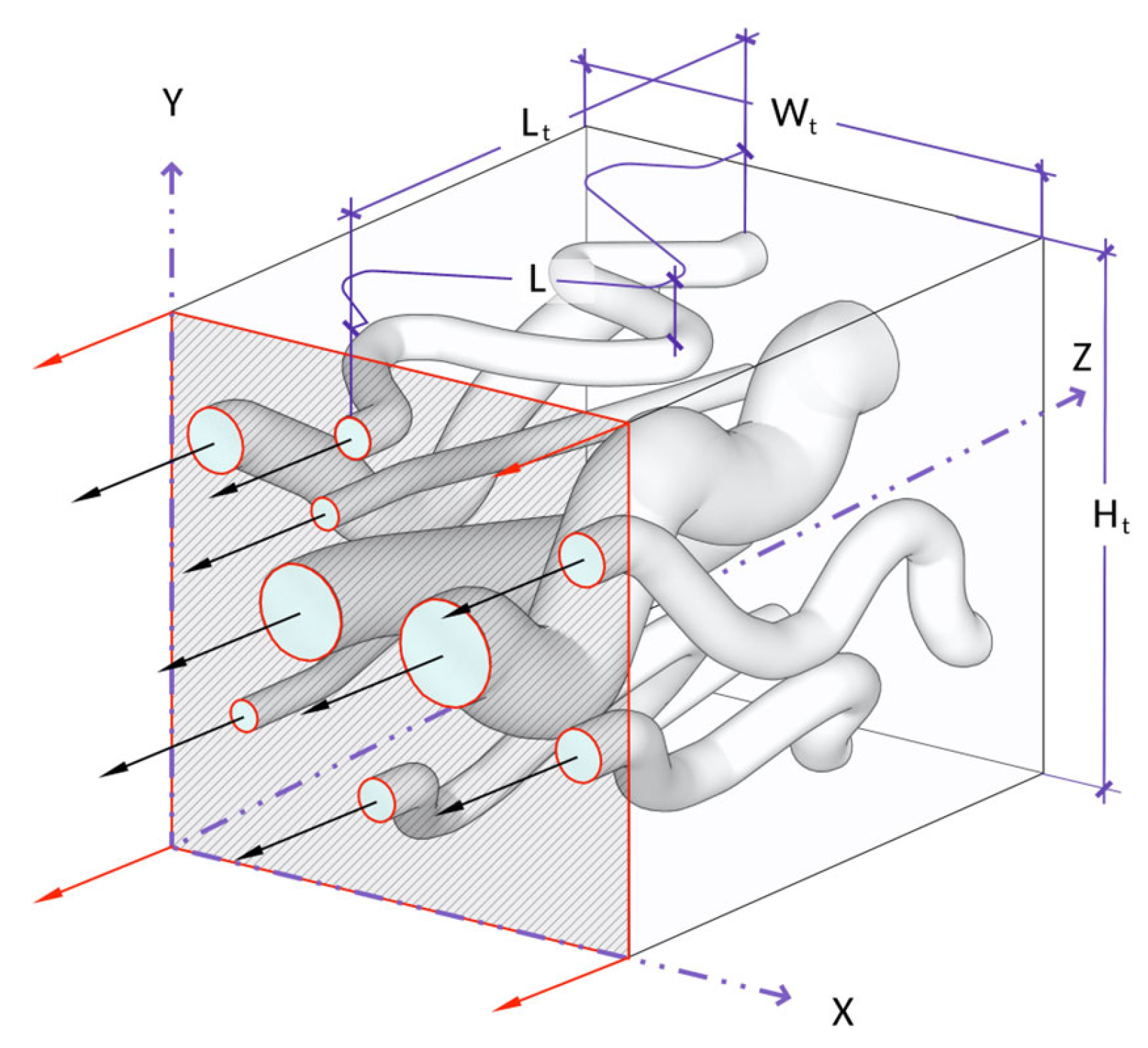
The behaviour of a porous medium can be described as an assemblage of parallel tortuous capillary tubes with varying radii [6], as shown in Figure A2. Assuming a capillary bundle, the total discharge, Q, of a porous medium is thus:

$$Q=N{\displaystyle \frac{\mathsf{\Delta }P{A_v}^2}{8\mathsf{\pi }\mu L_v}}$$

(A3)

where N is the total number of capillaries. Porosity of a porous medium can be defined as the ratio of void volume $Vv$ and total volume $Vt$:

$$\Phi ={\displaystyle \frac{V_v}{V_t}}$$

(A4)

Assuming that all capillary pores contribute to fluid conduction ($\Phi ={\Phi }_e)$, thus:

$${\Phi }_e=N{\displaystyle \frac{A_v{L}_v}{A_t{L}_t}}$$

(A5)

Incorporating tortuosity $\left(\tau \right)$ as a ratio of capillary length, $L_v$, and medium length, $L_t$, yields:

$$N ={\displaystyle \frac{{\Phi }_e A_t}{\tau A_v}}$$

(A6)

The flow of fluid through a porous medium as described by Darcy’s law [64]:

$$Q={\displaystyle \frac{\mathrm{k}{A}_t}{\mu L_t}} \mathsf{\Delta }P$$

(A7)

where $k$ is the intrinsic permeability of the medium. Substituting Equation (A6) into Equation (A3), then substituting with Equation (A7) yields:

$$k={\displaystyle \frac{{{\Phi }_{e}A}_v}{8{\mathsf{\pi }\tau }^2}}$$

(A8)

This formula defines the permeability of the porous medium as a function of porosity, pore cross-sectional area, and tortuosity of the flow path.

Figure A2. A capillary bundle with N number of interconnected capillaries all under the same pressure gradient from the porous medium with a volume of ${\mathrm{L}}_{\mathrm{t}}\times {\mathrm{H}}_{\mathrm{t}}\times {\mathrm{W}}_{\mathrm{t}}$.

Figure A2. A capillary bundle with N number of interconnected capillaries all under the same pressure gradient from the porous medium with a volume of ${\mathrm{L}}_{\mathrm{t}}\times {\mathrm{H}}_{\mathrm{t}}\times {\mathrm{W}}_{\mathrm{t}}$.

Appendix A.3. Coupling of Electrical and Hydraulic Properties

To link the hydraulic permeability and pore physics with electrical properties, we must revisit Ohm’s law. In the context of electromagnetic theory and continuum physics, Ohm’s law is expressed in its local differential form as:

$$J=\sigma E$$

(A9)

where $J$ is the current density vector, $\sigma$ is the electrical conductivity of the medium, and $E$ is the electric field intensity.

The electrical conductivity is described by the five-phase model, which terms the total observed electrical conductivity $\left({\sigma }_t\right)$ as the sum function of pore-fluid conductivity ${(\sigma }_{pf})$, solid-fluid conductivity (${\sigma }_{sf})$, grain matrix conductivity (${\sigma }_g)$, ion-exchange conductivity (${\sigma }_i)$, and Maxwellian-effects conductivity (${\sigma }_m)$ [14].

$${\sigma }_t={\sigma }_{pf}+{\sigma }_{sf}+{\sigma }_g+{\sigma }_i+{\sigma }_m$$

(A10)

In a saturated porous medium, the bulk electrical conductivity (${\sigma }_b)$ arises from three principal mechanisms: pore-fluid conduction, ionic exchange, and solid–fluid interfacial conduction [4]. The conductivity of the pore fluid is primarily governed by the intrinsic electrical properties of the fluid itself. Since saline fluids contain a high concentration of dissolved ions that serve as mobile charge carriers, electrical conductivity increases proportionally with fluid salinity.

The ionic-exchange capacity of the solid matrix is an inherent property of the soil that reflects its ability to exchange ions with the surrounding solids and fluids and thereby facilitate charge transfer. The solid–fluid interfacial conduction mechanism is influenced by the clay mineral content and type, as well as by the distribution of charged ions at grain boundaries. This process is explained by the electrical double layer (EDL) [50,73].

Figure A3a shows that, in particles that do not form EDL, such as silica sand, the area of the total pore throat equals the effective area in which both fluid and electricity are conducted. In EDL-forming particles, as shown in Figure A3b, the effective pore throat area is just a fraction of the total pore throat, causing electricity and fluid flow paths to diverge. In EDL-forming media, the fluid flow is only a fraction of the electrical flow path, since only a small portion of that fluid is mobile.

Figure A3. (a) Non-EDL-forming particles and (b) EDL-forming interaction with fluid and electrical flow. In (a), the electrically neutral particle shows no ionic distribution or electrokinetic effects, with the pore throat area remaining unchanged. In (b), the particle surface attracts a compact layer of cations and a diffuse outer layer that decreases the pore throat area. Indicated particle types (i.e., sand and clay) are for illustration; any particle can have the capacity to form an EDL depending on its inherent properties.

Figure A3. (a) Non-EDL-forming particles and (b) EDL-forming interaction with fluid and electrical flow. In (a), the electrically neutral particle shows no ionic distribution or electrokinetic effects, with the pore throat area remaining unchanged. In (b), the particle surface attracts a compact layer of cations and a diffuse outer layer that decreases the pore throat area. Indicated particle types (i.e., sand and clay) are for illustration; any particle can have the capacity to form an EDL depending on its inherent properties.

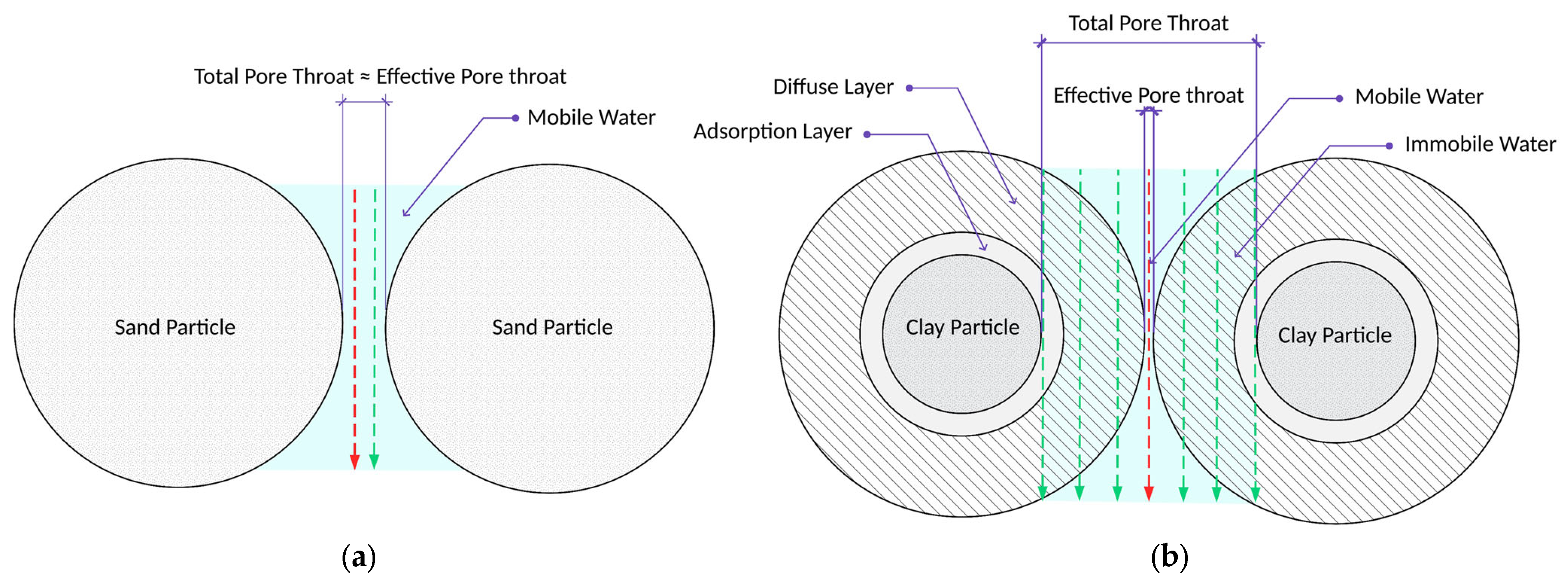
This sheds light on two primary facts. Firstly, despite the high percentage of saturated pores found in clay, the bulk of which contains immobile fluid; thus permeability approaches zero. Secondly, the high electrical conductivity of clay compared to other soils should be considered. While the immobile fluid does not contribute to fluid conduction, the free ions in the fluid conduct electrical current. This may be interpreted as a false positive when relating conductivity of electricity and fluids, making this understanding crucial.

Since the ionic-exchange capacity and solid–fluid conductivities are governed by the solid part of the matrix, they are combined in a single expression and denoted as solid or surface conductivity (${\sigma }_s)$ and pore-fluid conductivity as fluid conductivity (${\sigma }_f)$. Thus, by resolving Equation (A9) and writing the expression in terms of $I,$ current flow through a porous medium, under a voltage influence, $\Delta V$, yields:

$$I={\mathsf{\sigma }}_t{\mathrm{A}}_t{\displaystyle \frac{\mathsf{\Delta }\mathrm{V}}{{\mathrm{L}}_t}}$$

(A11)

Re-writing the expression in-terms of current flow with N number of capillaries where the current is mitigating through the saturated pore fluid $\left({\sigma }_w\right)$ in the capillary and the solid walls of the capillary $({\sigma }_s{\displaystyle )}$:

$$I=N ({\mathsf{\sigma }}_f+{\mathsf{\sigma }}_s){\mathrm{A}}_v{\displaystyle \frac{\mathsf{\Delta }\mathrm{V}}{{\mathrm{L}}_v}}$$

(A12)

Substituting Equation (A6) into (A12) and then equating it with (A11) yields:

$${\mathsf{\sigma }}_t={\displaystyle \frac{\Phi }{{\tau }^2}}{(\mathsf{\sigma }}_f+{\mathsf{\sigma }}_s)$$

(A13)

Equation (A13) describes the electrical conductivity as a subject of porosity divided by tortuosity and multiplied by the summation of fluid and solid conductivities. This formula has a striking similarity to Waxman and Smits’s model [4]; from that similarity, we can derive the expression ${\displaystyle \frac{\Phi }{{\tau }^2}}$ $=$ ${\Phi }^m$, where $m$ is the cementation exponent. With greater degrees of compaction and cementation, a significant decrease in porosity occurs, which forces the current to pass through longer and more tortuous passages. Solving Equation (A13) for porosity and substituting into Equation (A8) yields:

$$k= {\displaystyle \frac{A_v}{C }}{\displaystyle \frac{{\sigma }_t}{{ \sigma }_f+{\sigma }_s }}$$

(A14)

Equation (A14) expresses permeability as a function of the pore area and electrical conductivity. The constant $C$ equals to 8$\pi$ as long as the assumptions of the model stand. The model no longer describes a single pore, but a representative elementary volume (REV), which describes the total space occupied by pores. Therefore,$A_v$ becomes a REV-equivalent pore area that is effective for fluid conduction or equivalent effective pore area and denoted as $A_e$, and can be referred to as effective pore area, or effective pore throat area. These terms are interchangeable. The model can be rewritten in various forms. The first, by simply solving for permeability and noticing that the fracture ${\displaystyle \frac{{\sigma }_t}{{ \sigma }_f+{\sigma }_s }}$ is equivalent to ${\Phi }^m$ of Waxman–Smits model; thus:

$$\mathrm{k}= {\displaystyle \frac{G{A}_e}{C }}$$

(A15)

This expression describes permeability as a function of electrical connectedness, $G,$ in a porous medium, where $G$ is the reciprocal of the formation factor, $F \left[22\right]$. The terms ${\Phi }^m$ and $G$ are interchangeable.

Earlier, we established that ${\Phi }^m$ is equivalent to ${\displaystyle \frac{\Phi }{{\tau }^2}}$ and, to recast tortuosity as a measure of path connectivity effort rather than transport resistance, and to unify the description of electrical and hydraulic flow paths, a new coefficient is introduced. Termed flowability, this coefficient characterises the efficiency at which connected pores facilitate transport. Flowability is defined as the inverse of the squared tortuosity, ${\tau }^{ -2}$, and is symbolised by Ƒ. As a bounded quantity between 0 and 1, flowability represents the squared ratio of the effective transport length to the total length of the porous medium, providing a common geometric descriptor applicable to both electrical conduction and fluid flow. Thus:

$$\mathrm{k}= {\displaystyle \frac{1}{C }}\Phi A_e \mathrm{Ƒ}$$

(A16)

References

- Archie, G.E. The electrical resistivity log as an aid in determining some reservoir characteristics. Trans. AIME 1942, 146, 54–62. [Google Scholar] [CrossRef] [Scilit]
- Maillet, R. The fundamental equations of electrical prospecting. Geophysics 1947, 12, 529–556. [Google Scholar] [CrossRef] [Scilit]
- Carman, P.C. Flow of Gases Through Porous Media; Butterworths: London, UK, 1956. [Google Scholar]
- Waxman, M.H.; Smits, L.J.M. Electrical conductivities in oil-bearing shaly sands. Soc. Pet. Eng. J. 1968, 8, 107–122. [Google Scholar] [CrossRef] [Scilit]
- Bear, J. Dynamics of Fluids in Porous Media; Elsevier: New York, NY, USA, 1972. [Google Scholar]
- Dullien, F.A.L. Porous Media: Fluid Transport and Pore Structure, 2nd ed.; Academic Press: San Diego, CA, USA, 1992. [Google Scholar]
- Bussian, A.E. Electrical conductance in a porous medium. Geophysics 1983, 48, 1258–1268. [Google Scholar] [CrossRef] [Scilit]
- Johnson, D.L.; Koplik, J.; Schwartz, L.M. New pore-size parameter characterizing transport in porous media. Phys. Rev. Lett. 1986, 57, 2564–2567. [Google Scholar] [CrossRef] [Scilit]
- Katz, A.J.; Thompson, A.H. Quantitative prediction of permeability in porous rock. Phys. Rev. B 1986, 34, 8179–8181. [Google Scholar] [CrossRef] [Scilit]
- Sen, P.N.; Goode, P.A.; Sibbit, A. Electrical conduction in clay bearing sandstones at low and high salinities. J. Appl. Phys. 1988, 63, 4832–4840. [Google Scholar] [CrossRef] [Scilit]
- Bernabé, Y. The transport properties of networks of cracks and pores. J. Geophys. Res. Solid Earth 1995, 100, 4231–4241. [Google Scholar] [CrossRef] [Scilit]
- Revil, A.; Cathles, L.M., III. Permeability of shaly sands. Water Resour. Res. 1999, 35, 651–662. [Google Scholar] [CrossRef] [Scilit]
- Weller, A.; Slater, L.; Nordsiek, S. On the relationship between induced polarization and surface conductivity: Implications for petrophysical interpretation of electrical measurements. Geophysics 2013, 78, D315–D325. [Google Scholar] [CrossRef] [Scilit]
- Salem, H.S. The compressional to shear-wave velocity ratio for surface soils and shallow sediments. Eur. J. Environ. Eng. Geophys. 2000, 5, 3–14. [Google Scholar]
- Glover, P.W.J.; Wei, W.; Lorinczi, P. Connectedness theory of relative permeability. Transp. Porous Media 2025, 152, 86. [Google Scholar] [CrossRef] [Scilit]
- Ohm, G.S. Die Galvanische Kette, Mathematisch Bearbeitet; J.G.F. Kniestädt: Berlin, Germany, 1827. [Google Scholar]
- Darcy, H. Les Fontaines Publiques de la Ville de Dijon; Victor Dalmont: Paris, France, 1856. [Google Scholar]
- Thanh, L.D.; Jougnot, D.; Solazzi, S.G.; Luo, H.; Nguyen, M.H.; Nguyen, V.N.; Do, P.V.; Luong, T.T.H. Relating permeability and electrical conductivity in partially saturated porous media by means of the Johnson–Koplik–Schwartz characteristic length. Geophys. J. Int. 2024, 237, 1157–1173. [Google Scholar] [CrossRef] [Scilit]
- Nguyen, M.H.; Jougnot, D.; Thanh, L.D.; Guarracino, L.; Dang, T.M.H.; Tran, T.C.T.; Vu, V.T. A model for estimating the permeability of porous media from the critical pore radius. Hydrogeol. J. 2025, 33, 1529–1540. [Google Scholar] [CrossRef] [Scilit]
- Carbonari, R.; Salone, R.; Di Maio, R. Predicting electrical resistivity in natural degassing geological systems through petrophysical and thermodynamic data: A machine learning approach. Pure Appl. Geophys. 2025, 183, 1177–1201. [Google Scholar] [CrossRef] [Scilit]
- Reuss, F.F. Sur un nouvel effet de l’électricité galvanique. Mém. Soc. Impériale Nat. Moscou 1809, 2, 327–337. [Google Scholar]
- Glover, P.W.J. What is the cementation exponent? A new interpretation. Lead. Edge 2009, 28, 82–85. [Google Scholar] [CrossRef] [Scilit]
- Esmaeilpour, M.; Ghanbarian, B.; Liang, F.; Liu, H.H. Scale-dependent permeability and formation factor in porous media: Applications of percolation theory. Fuel 2021, 301, 121090. [Google Scholar] [CrossRef] [Scilit]
- Vereecken, H.; Amelung, W.; Bauke, S.L.; Bogena, H.; Brüggemann, N.; Montzka, C.; Vanderborght, J.; Bechtold, M.; Blöschl, G.; Carminati, A.; et al. Soil hydrology in the Earth system. Nat. Rev. Earth Environ. 2022, 3, 573–587. [Google Scholar] [CrossRef] [Scilit]
- Saxton, K.E.; Rawls, W.J. Soil water characteristic estimates by texture and organic matter for hydrologic solutions. Soil Sci. Soc. Am. J. 2006, 70, 1569–1578. [Google Scholar] [CrossRef] [Scilit]
- Peters, A.; Iden, S.C.; Durner, W. Prediction of absolute unsaturated hydraulic conductivity—Comparison of four different capillary bundle models. Hydrol. Earth Syst. Sci. 2023, 27, 4579–4593. [Google Scholar] [CrossRef] [Scilit]
- Jarvis, N.J. A review of non-equilibrium water flow and solute transport in soil macropores: Principles, controlling factors and consequences for water quality. Eur. J. Soil Sci. 2007, 58, 523–546. [Google Scholar] [CrossRef] [Scilit]
- Iden, S.C.; Peters, A.; Durner, W. Improving prediction of hydraulic conductivity by constraining capillary bundle models to a maximum pore size. Adv. Water Resour. 2015, 85, 86–92. [Google Scholar] [CrossRef] [Scilit]
- Bonetti, S.; Wei, Z.; Or, D. A framework for quantifying hydrologic effects of soil structure across scales. Commun. Earth Environ. 2021, 2, 107. [Google Scholar] [CrossRef] [Scilit]
- Szabó, B.; Weynants, M.; Weber, T.K.D. Updated European hydraulic pedotransfer functions with communicated uncertainties in the predicted variables (euptfv2). Geosci. Model Dev. 2021, 14, 151–175. [Google Scholar] [CrossRef] [Scilit]
- Blanchy, G.; Albrecht, L.; Bragato, G.; Garré, S.; Jarvis, N.; Koestel, J. Impacts of soil management and climate on saturated and near-saturated hydraulic conductivity: Analyses of the Open Tension-disk Infiltrometer Meta-database (OTIM). Hydrol. Earth Syst. Sci. 2023, 27, 2703–2724. [Google Scholar] [CrossRef] [Scilit]
- Ahuja, L.R.; Cassel, D.K.; Bruce, R.R.; Barnes, B.B. Evaluation of spatial distribution of hydraulic conductivity using effective porosity data. Soil Sci. 1989, 148, 404–411. [Google Scholar] [CrossRef] [Scilit]
- Leys, C.; Ley, C.; Klein, O.; Bernard, P.; Licata, L. Detecting outliers: Do not use standard deviation around the mean, use absolute deviation around the median. J. Exp. Soc. Psychol. 2013, 49, 764–766. [Google Scholar] [CrossRef] [Scilit]
- Cosby, B.J.; Hornberger, G.M.; Clapp, R.B.; Ginn, T.R. A statistical exploration of the relationships of soil moisture characteristics to the physical properties of soils. Water Resour. Res. 1984, 20, 682–690. [Google Scholar] [CrossRef] [Scilit]
- Saxton, K.E.; Rawls, W.J.; Romberger, J.S.; Papendick, R.I. Estimating generalized soil-water characteristics from texture. Soil Sci. Soc. Am. J. 1986, 50, 1031–1036. [Google Scholar] [CrossRef] [Scilit]
- Brakensiek, D.L.; Rawls, W.J.; Stephenson, G.R. Modifying SCS hydrologic soil groups and curve numbers for rangeland soils. In ASAE Paper No. PNR-84-203; American Society of Agricultural Engineers: St. Joseph, MI, USA, 1984. [Google Scholar]
- Ferrer Julià, M.; Estrela Monreal, T.; Sánchez del Corral Jiménez, A.; García Meléndez, E. Constructing a saturated hydraulic conductivity map of Spain using pedotransfer functions and spatial prediction. Geoderma 2004, 123, 257–277. [Google Scholar] [CrossRef] [Scilit]
- Puckett, W.E.; Dane, J.H.; Hajek, B.F. Physical and mineralogical data to determine soil hydraulic properties. Soil Sci. Soc. Am. J. 1985, 49, 831–836. [Google Scholar] [CrossRef] [Scilit]
- Dane, J.H.; Puckett, W.E. Field soil hydraulic properties based on physical and mineralogical information. In Indirect Methods for Estimating the Hydraulic Properties of Unsaturated Soils; van Genuchten, M.T., Leij, F.J., Lund, L.J., Eds.; University of California: Riverside, CA, USA, 1992; pp. 389–403. [Google Scholar]
- Campbell, G.S.; Shiozawa, S. Prediction of hydraulic properties of soils using particle-size distribution and bulk density data. In Indirect Methods for Estimating the Hydraulic Properties of Unsaturated Soils; van Genuchten, M.T., Leij, F.J., Lund, L.J., Eds.; University of California: Riverside, CA, USA, 1992; pp. 317–328. [Google Scholar]
- Draper, N.R.; Smith, H. Applied Regression Analysis, 3rd ed.; Wiley: New York, NY, USA, 1998. [Google Scholar] [CrossRef] [Scilit]
- Pearson, K., VII. Note on regression and inheritance in the case of two parents. Proc. R. Soc. Lond. 1895, 58, 240–242. [Google Scholar] [CrossRef] [Scilit]
- Spearman, C. The proof and measurement of association between two things. Am. J. Psychol. 1904, 15, 72–101. [Google Scholar] [CrossRef] [Scilit]
- Clark, M.P.; Vogel, R.M.; Lamontagne, J.R.; Mizukami, N.; Knoben, W.J.M.; Tang, G.; Gharari, S.; Freer, J.E.; Whitfield, P.H.; Shook, K.R.; et al. The abuse of popular performance metrics in hydrologic modeling. Water Resour. Res. 2021, 57, e2020WR029001. [Google Scholar] [CrossRef] [Scilit]
- Rubinstein, R.Y.; Kroese, D.P. Simulation and the Monte Carlo Method, 3rd ed.; Wiley: Hoboken, NJ, USA, 2016. [Google Scholar] [CrossRef] [Scilit]
- Iman, R.L.; Conover, W.J. A distribution-free approach to inducing rank correlation among input variables. Commun. Stat. Simul. Comput. 1982, 11, 311–334. [Google Scholar] [CrossRef] [Scilit]
- Buckingham, E. On physically similar systems; illustrations of the use of dimensional equations. Phys. Rev. 1914, 4, 345–376. [Google Scholar] [CrossRef] [Scilit]
- Sahimi, M. Flow and Transport in Porous Media and Fractured Rock, 2nd ed.; Wiley-VCH: Weinheim, Germany, 2011. [Google Scholar] [CrossRef] [Scilit]
- Revil, A.; Glover, P.W.J. Theory of ionic-surface electrical conduction in porous media. Phys. Rev. B 1997, 55, 1757–1773. [Google Scholar] [CrossRef] [Scilit]
- Chapman, D.L.L.I. A contribution to the theory of electrocapillarity. Philos. Mag. 1913, 25, 475–481. [Google Scholar] [CrossRef] [Scilit]
- Lu, X. Fluid Flow and Heat Transfer in Porous Media Manufactured by a Space Holder Method. Ph.D. Thesis, University of Liverpool, Liverpool, UK, 2020. [Google Scholar]
- Hong, B.; Li, X.; Wang, L.; Li, L.; Xue, Q.; Meng, J. Using the effective void ratio and specific surface area in the Kozeny–Carman equation to predict the hydraulic conductivity of loess. Water 2020, 12, 24. [Google Scholar] [CrossRef] [Scilit]
- Kostek, S.; Schwartz, L.M.; Johnson, D.L. Fluid permeability in porous media: Comparison of electrical estimates with hydrodynamical calculations. Phys. Rev. B 1992, 45, 186–195. [Google Scholar] [CrossRef] [Scilit]
- Marion, D.; Nur, A.; Yin, H.; Han, D. Compressional velocity and porosity in sand-clay mixtures. Geophysics 1992, 57, 554–563. [Google Scholar] [CrossRef] [Scilit]
- Paschalis, A.; Bonetti, S.; Guo, Y.; Fatichi, S. On the uncertainty induced by pedotransfer functions in terrestrial biosphere modeling. Water Resour. Res. 2022, 58, e2021WR031871. [Google Scholar] [CrossRef] [Scilit]
- Dix, M.; Manca, G.; Okafor, K.C.; Borrison, R.; Kirchheim, K.; Sharma, D.; Chandrika, K.; Maduskar, D.; Ortmeier, F. Measuring the robustness of ML models against data quality issues in industrial time series data. In Proceedings of the 2023 IEEE 21st International Conference on Industrial Informatics (INDIN), Lemgo, Germany, 17–20 July 2023; pp. 1–8. [Google Scholar] [CrossRef] [Scilit]
- Sales, D.d.S.; Lugon Junior, J.; Costa, D.d.A.; Sales, R.S.B.; Neves, R.J.; Silva Neto, A.J.d. Sensitivity analysis of soil hydraulic parameters for improved flow predictions in an Atlantic Forest watershed using the MOHID-Land platform. Eng 2025, 6, 65. [Google Scholar] [CrossRef] [Scilit]
- Chen, J.; Tong, H.; Yuan, J.; Fang, Y.; Gu, R. Permeability prediction model modified on Kozeny–Carman for building foundation of clay soil. Buildings 2022, 12, 1798. [Google Scholar] [CrossRef] [Scilit]
- Lehmann, P.; Leshchinsky, B.; Gupta, S.; Mirus, B.B.; Bickel, S.; Lu, N.; Or, D. Clays are not created equal: How clay mineral type affects soil parameterization. Geophys. Res. Lett. 2021, 48, e2021GL095311. [Google Scholar] [CrossRef] [Scilit]
- Luo, M.; Qin, Q.; Wang, S.; Pan, L.; Li, H. Water-quality thresholds and formation-damage mechanisms during water injection in the southern area of the deep reservoir in the Gaoshangpu oilfield. J. Geo-Energy Environ. 2026, 2, 230–243. [Google Scholar] [CrossRef] [Scilit]
- Emelianov, V.; Zhang, Z.; Weller, A.; Halisch, M.; Titov, K. Surface conductivity of clays. Geophys. J. Int. 2024, 238, 1013–1026. [Google Scholar] [CrossRef] [Scilit]
- Amiri, S.; Bayat, A.; Akbari, S. Swelling characteristics of various clays in presence of an aqueous environment under different conditions. Colloids Surf. A Physicochem. Eng. Asp. 2025, 707, 135942. [Google Scholar] [CrossRef] [Scilit]
- Carman, P.C. Fluid flow through granular beds. Trans. Inst. Chem. Eng. 1937, 15, 150–166. [Google Scholar]
- Muskat, M. The Flow of Homogeneous Fluids Through Porous Media; McGraw-Hill: New York, NY, USA, 1937. [Google Scholar]
- Jacob, C.E. On the flow of water in an elastic artesian aquifer. Eos Trans. AGU 1940, 21, 574–586. [Google Scholar] [CrossRef] [Scilit]
- Grunwald, S.; Harris, W.G.; Hurt, W.; Bloom, S.A.; Deich, W.; Hoover, B.; Bloom, K. Florida Soil Characterization Data; Technical Report; Soil and Water Science Department, IFAS, University of Florida: Gainesville, FL, USA, 2020. [Google Scholar]
- Gupta, S.; Hengl, T.; Lehmann, P.; Bonetti, S.; Or, D. SoilKsatDB: Global database of soil saturated hydraulic conductivity measurements for geoscience applications. Earth Syst. Sci. Data 2021, 13, 1593–1612. [Google Scholar] [CrossRef] [Scilit]
- Rahmati, M.; Weihermüller, L.; Vanderborght, J.; Pachepsky, Y.A.; Mao, L.; Sadeghi, S.H.; Moosavi, N.; Kheirfam, H.; Montzka, C.; Van Looy, K.; et al. Development and analysis of the Soil Water Infiltration Global database. Earth Syst. Sci. Data 2018, 10, 1237–1263. [Google Scholar] [CrossRef] [Scilit]
- Lehner, B.; Grill, G. Global river hydrography and network routing: Baseline data and new approaches to study the world’s large river systems. Hydrol. Process. 2013, 27, 2171–2186. [Google Scholar] [CrossRef] [Scilit]
- Nemes, A.; Schaap, M.G.; Leij, F.J.; Wösten, J.H.M. Description of the unsaturated soil hydraulic database UNSODA version 2.0. J. Hydrol. 2001, 251, 151–162. [Google Scholar] [CrossRef] [Scilit]
- Vereecken, H.; Van Looy, K.; Weynants, M.; Javaux, M. Soil Retention and Conductivity Curve Data Base sDB, Link to MATLAB Files [Data set]; PANGAEA, 2017. [Google Scholar] [CrossRef]
- Poiseuille, J.L.M. Recherches expérimentales sur le mouvement des liquides dans les tubes de très petits diamètres. Mém. Présentés Divers Savants Acad. R. Sci. Inst. Fr. 1846, 9, 433–544. [Google Scholar]
- Gouy, G. Sur la constitution de la charge électrique à la surface d’un électrolyte. J. Phys. Théor. Appl. 1910, 9, 457–468. [Google Scholar] [CrossRef] [Scilit]
Disclaimer/Publisher’s Note: The statements, opinions and data contained in all publications are solely those of the individual author(s) and contributor(s) and not of MDPI and/or the editor(s). MDPI and/or the editor(s) disclaim responsibility for any injury to people or property resulting from any ideas, methods, instructions or products referred to in the content. |
© 2026 by the authors. Licensee MDPI, Basel, Switzerland. This article is an open access article distributed under the terms and conditions of the Creative Commons Attribution (CC BY) license.