


Abstract
On 20 April 2026 at 07:52:58 UTC, an Mw 7.4 earthquake struck offshore Miyako, northeastern Japan. We investigated the resulting coseismic ionospheric disturbances (CIDs) using 1 Hz multi-frequency GNSS observations and ionosonde measurements. Slant total electron content derived from L1–L2, L1–L5, and L2–L5 combinations was detrended using a Savitzky–Golay filter and band-pass filtered at 2–10 min. Directional hodochrone analysis showed strong azimuthal anisotropy, with the observed perturbations propagating at apparent horizontal velocities of 0.41–1.92 km s−1 across four sectors, substantially below typical Rayleigh-wave-associated CID velocities. The observed timing and waveform characteristics are consistent with vertically excited acoustic disturbances sampled obliquely by the GNSS links. Independent ionosonde observations at Wakkanai, Icheon, and Okinawa demonstrated Multiple Cusp Signatures in the bottomside F-region within 12–17 min, with decreasing cusp sharpness toward lower latitudes. Geomagnetic and solar indices indicate relatively quiet conditions during the observations, reducing the likelihood of contamination by disturbances driven by space weather. The results enrich our understanding on coseismic ionospheric disturbances in the Mw 7–7.5 range, showing that moderate subduction earthquakes can produce direction-dependent ionospheric signatures, with apparent velocities lower than typical Rayleigh-wave-associated CID velocities, detectable through combined GNSS-TEC and ionosonde monitoring.
1. Introduction
Earthquake-induced ionospheric disturbances provide a direct observational window into lithosphere–atmosphere–ionosphere coupling, because seismic forcing launches atmospheric waves that perturb ionospheric electron density and become measurable through GNSS total electron content (TEC) and ionosonde observations [1,2,3]. These coseismic ionospheric disturbances (CIDs) have been documented following earthquakes across a broad magnitude range, from very severe events such as the 2010 Chile and 2011 Tohoku-oki earthquakes to moderate events including the 1999 Chi-Chi, 2015 Gorkha, 2020 Jamaica, 2020 Samos, 2023 Turkey, and 2025 Myanmar earthquakes [1,2,4,5,6,7,8,9,10,11,12]. Their significance extends beyond upper-atmospheric phenomenology. Near-field CIDs can capture information on coseismic vertical deformation and rupture development, whereas far-field signatures can trace the propagation of seismic, acoustic, and gravity wave energy through the atmosphere, together with tsunami-driven wave energy where the causative earthquake generates a tsunami [1,13,14,15]. The character of the ionospheric response may also provide information on the source process, as slow, tsunamigenic fault slip has been shown to preferentially excite longer-period atmospheric gravity waves rather than short-period acoustic waves [16]. This coupling has practical relevance for geohazard monitoring and space-weather-aware observing systems because CIDs can be detected within minutes of major earthquakes and, under favourable conditions, before the arrival of tsunami waves at exposed coastlines [6,15,17].
The physical basis of coseismic ionospheric perturbations is now well-established. Strong shallow earthquakes produce abrupt surface displacement and atmospheric compression near the ground; as these disturbances propagate upward through an exponentially decreasing neutral density, their amplitudes grow and they couple efficiently to ionospheric plasma through neutral–ion interactions [2]. In the near field, the dominant signatures are usually attributed to acoustic or shock-acoustic waves generated by coseismic vertical crustal motion, whereas additional components can be generated by propagating Rayleigh waves, at longer periods and larger distances, by tsunami-driven atmospheric gravity waves [1,6,9,18]. Different excitation mechanisms also differ in arrival time, propagation speed, duration, and waveform morphology, which is why separating acoustic responses from mixed-mode post-seismic disturbances remains a central problem in ionospheric seismology [1,2,6,19].
GNSS-TEC observations are a powerful tool for coseismic earthquake studies because dense receiver networks resolve CID evolution with high temporal and spatial fidelity [6,14,16]. Since the first GPS-based detections, many subsequent studies have shown that initial acoustic-wave CIDs typically emerge about 7–15 min after earthquake origin time, with dominant periods near 4 min and horizontal propagation speeds close to the sound speed at F-region heights, commonly ~0.8–1.5 km s−1 [16,18,20,21]. Exceptional cases also show faster apparent near-field propagation, interpreted as shock-acoustic behaviour or the contribution of Rayleigh-wave-related acoustic excitation; for the 2011 Tohoku-oki earthquake, first arrival was detected ~464 s after rupture and subsequent propagation reached ~1.3–1.5 km s−1, while other analyses resolved Rayleigh-related components at ~2–4 km s−1 or faster [2,5,6,16].
Waveform morphology likewise contains source and propagation information, but it is less uniform than simple travel-time scaling suggests. Near-field coseismic TEC signatures can appear as impulsive enhancements followed by depletions, standard or inverse N-type waveforms, concentric wave trains with multiple negative peaks, or longer-lived oscillations near the epicentral region [18,21]. Polarity and shape depend not only on the earthquake source but also on whether coseismic uplift and subsidence coexist, as illustrated by contrasting positive and negative CID responses in the 2016 West Sumatra and 2018 Palu earthquakes [20]. This morphological variability is one reason why CID interpretation cannot rely on amplitude alone and instead requires joint consideration of timing, frequency content, and spatial coherence [14]. A second well-established fact is that CID propagation is rarely isotropic. Evidence from the 2004 Sumatra, 2011 Tohoku, 2015 Gorkha, 2022 Mexico, 2023 Turkey, and 2021 Alaska earthquake demonstrates pronounced azimuthal variations in amplitude, velocity, and detectability [2,9,18,19,21,22]. Part of this asymmetry reflects source characteristics, including rupture directivity, fault strike, focal mechanism, and the spatial distribution of coseismic vertical displacement [9,13,21]. However, non-tectonic factors are also crucial. The orientation of the geomagnetic field, the line-of-sight geometry between the receiver and satellite, and background electron-density gradients can reshape the apparent CID field and even bias inferences regarding the underlying earthquake source [9,13,22]. The ambient ionospheric state, whether geomagnetically quiet or disturbed, can further modulate the characteristics of CID propagation, as pre-existing gradients in electron density and thermospheric composition influence neutral–ion coupling efficiency and the background sound-speed structure along the wave path [9].
These advances have clarified the main phenomenology of coseismic ionospheric forcing, but several limitations remain, especially for short-period perturbations. First, many events exhibit a superposition of acoustic, gravity-wave, Rayleigh-wave, and tsunami-related signatures, making it difficult to isolate the initial short-period response and to compare waveform properties consistently between earthquakes [2,9,14]. Second, the relation between CID characteristics and earthquake source properties remains only partly constrained. Slow-fault-slip signatures appear to amplify long-period internal gravity waves more than short-period acoustic waves, whereas ordinary megathrust events show different scaling, implying that rupture timescale matters but not in the same way for all atmospheric modes [16]. Third, detectability itself depends strongly on event magnitude, depth, focal mechanism, atmospheric state, and observing geometry [9]. Even in dense networks, robust extraction of coherent CID wave packets from short-term TEC variability often requires specialized time–frequency or coherence-based approaches rather than simple visual inspection [14]. Complementary advances continue to extend this toolkit: coupled neutral–ion analytical frameworks now reproduce line-of-sight-dependent TEC responses to acoustic-gravity-wave forcing [23], while high-frequency Doppler-sounding arrays have detected seismo-acoustic signatures at distances where co-located GNSS-TEC and magnetometer responses remain below detection threshold [24].
These challenges are especially evident in the Japanese subduction zone, where the comprehensive documentation of the 2011 Tohoku-oki earthquake established a reference framework for subsequent studies while underscoring persistent uncertainties in the characteristics and mechanisms of coseismic ionospheric perturbations. GEONET revealed sudden TEC depletions after small impulsive enhancements, concentric waves spanning velocities from ~138 m s−1 to >3 km s−1, zonally elongated structures, and persistent short-period oscillations near the source region [18]. Independent analyses further showed a disk-shaped or rectangular ionospheric source region displaced from the epicentre, rapid first arrivals, long-distance southward propagation toward Taiwan, and rotation of the disturbance wave vector during propagation [5,6,22]. Yet Tohoku was an extreme Mw 9 class event, and its complexity does not automatically translate to more moderate but still tsunamigenic subduction earthquakes. Comprehensive analyses targeting recent Japanese events of smaller magnitude, with explicit emphasis on the short-period CID component and its spatial variability, remain comparatively scarce in the literature represented here [13,18,22].
The 20 April 2026 Mw 7.4 Miyako earthquake provides an opportunity to examine the short-period coseismic ionospheric perturbations (CIDs) associated with a major subduction event in the Japan Trench system. Unlike the extensively documented Mw 9.0 Tohoku-oki and Mw 8.8 Kamchatka earthquakes, whose extreme energy release and superposed acoustic, Rayleigh-wave, and tsunami-driven wavefields complicate isolation of the short-period acoustic response, the Miyako earthquake falls within the more frequent but comparatively under-characterized Mw 7–7.5 class, for which combined GNSS-TEC and ionosonde documentation of short-period CIDs and their azimuthal dependence remains scarce. This intermediate-magnitude setting offers a more tractable basis for isolating source- and geometry-dependent controls on short-period CID propagation than great (Mw ≥ 8.5) subduction earthquakes do. In this setting, near-field CID generation is sensitive to coseismic vertical deformation, while the observed ionospheric response may be modulated by rupture directivity, geomagnetic-field orientation, and satellite–receiver geometry [13]. Here, we investigate the ionospheric response to the Miyako earthquake using complementary multi-GNSS total electron content (TEC) measurements and ionograms. We characterize the spatial distribution, characteristic (peak) disturbance times, waveform morphology, dominant periods, and propagation characteristics of the observed perturbations, with particular emphasis on Multiple Cusp Signatures. By integrating GNSS-derived TEC perturbations with ionosonde observations, we provide a detailed characterization of the short-period coseismic ionospheric response to this intermediate-magnitude subduction earthquake and assess the propagation characteristics and spatial variability of the associated disturbances.
2. Materials and Methods
2.1. Seismological Setting
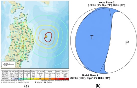
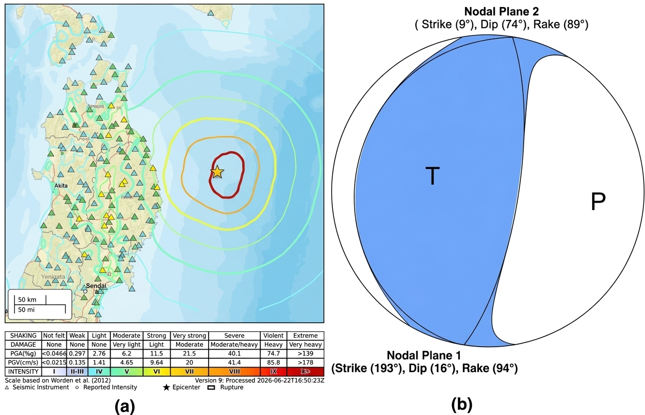
On 20 April 2026 at 07:52:58 UTC, a Mw 7.4 earthquake occurred offshore of Miyako, Iwate Prefecture, northeastern Japan (39.97° N, 143.059° E; Figure 1), within the Japan Trench subduction zone, where the Pacific Plate underthrusts northeastern Honshu. According to the USGS moment-tensor solution, the earthquake occurred at a depth of 25.0 km and had a scalar seismic moment of 2.01 × 1027 dyne cm (equivalent to 2.01 × 10²⁰ N m), with a reported half-duration of 13.3 s.
Figure 1.
(a) USGS ShakeMap for the 20 April 2026 Mw 7.4 earthquake offshore of Miyako, Japan (https://earthquake.usgs.gov/earthquakes/eventpage/us6000sri7/shakemap/intensity (accessed on 4 August 2026)). Coloured contour lines denote 1 MMI-unit increments (maximum ≈ VII near the epicentre, based on visual correlation with the intensity legend), triangles denote seismic stations, and the star marks the earthquake epicentre. (b) Lower-hemisphere focal-mechanism diagram for nodal planes 1 and 2 of the Mw 7.4 moment-tensor (https://earthquake.usgs.gov/earthquakes/eventpage/us6000sri7/moment-tensor (accessed on 4 August 2026)). Blue and white quadrants denote compressional and dilatational P-wave first-motion polarities, respectively, while the P and T axes indicate the compressional and tensional principal axes of the moment tensor.
Moment-tensor inversion yielded an Mw 7.4 solution with normalized tensor components of 0.795, −0.023, −0.772, 0.646, 1.730, and −0.180 (exponent 1027 dyne cm). The two nodal planes have strikes of 186° and 20°, dips of 12° and 78°, and rake angles of 76° and 93°, respectively, indicating a predominantly thrusting mechanism consistent with compressional deformation at the subduction interface. The modeled ground-motion intensity distribution (Figure 1) indicates strong-to-very-strong shaking along the nearest coastline, decreasing to weak-to-light shaking farther inland toward Sendai, consistent with an offshore interplate rupture in the Japan Trench system.
2.2. GNSS TEC Processing and Propagation Analysis
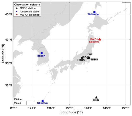
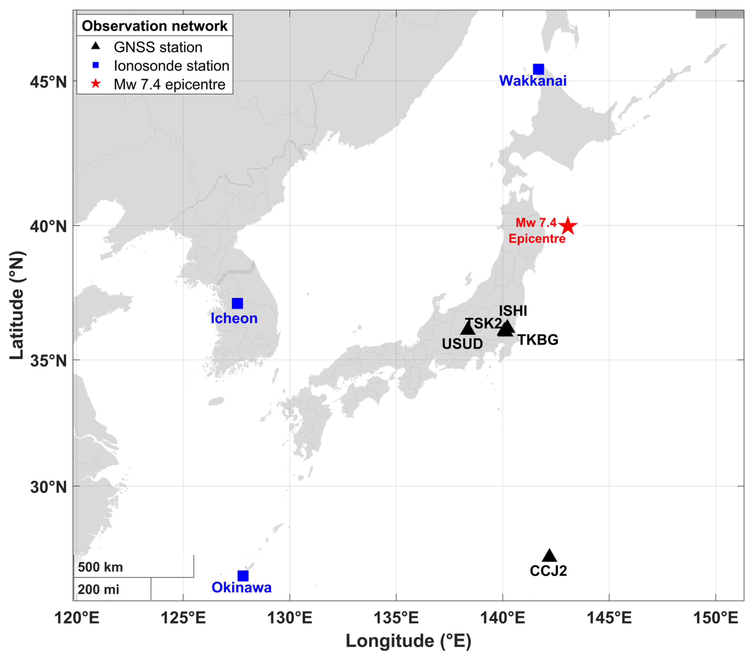
Coseismic ionospheric disturbances were investigated using high-rate (1 Hz) dual- and triple-frequency GNSS observations from five continuously operating stations distributed across Honshu and the Ogasawara Islands (USUD, TSK2, TKBG, ISHI and CCJ2; Figure 2, Table 1). For each station, RINEX observation files were processed with tec-suite (version 0.7.8) [25] to derive slant TEC (sTEC) along the receiver–satellite line of sight from the geometry-free combination of dual-frequency carrier-phase observables. The specific frequency pairs used (L1–L2, L1–L5 and L2–L5) depend on the tracked constellation and were exploited by tec-suite (version 0.7.8) to construct sTEC series for the 11 station–satellite links analyzed in this study.
Figure 2.
Geographic distribution of the instruments used to investigate the ionospheric response to the 20 April 2026 Mw 7.4 Miyako earthquake. Black triangles denote GNSS receivers, blue squares denote ionosonde stations, and the red star marks the earthquake epicentre.
Table 1.
Regional GNSS and ionosonde station network used in this study.
The derived sTEC series were processed to isolate short-period coseismic ionospheric perturbations (CIDs) from the slowly varying TEC background. A Savitzky–Golay filter (linear, first-order polynomial, applied within a centered sliding window of approximately 30.5 min) was applied to each sTEC series to estimate the slowly varying background component. This background was subtracted from original sTEC observations to obtain detrended TEC (dTEC). The detrended series were then filtered using a fourth-order Butterworth band-pass filter with passband periods of 2–10 min. Zero-phase forward and reverse filtering was applied to minimize phase distortion and preserve spatial information on the perturbations. The resulting band-passed dTEC series formed the basis for characterizing the short-period CID signatures, including their characteristic (peak) disturbance time, waveform morphology, dominant periods, and propagation characteristics. Missing samples, where present, were linearly interpolated before filtering to ensure continuous time series. Station–satellite links were retained only when a continuous, N-shaped dTEC perturbation could be clearly distinguished from the pre-event noise background within the expected acoustic-wave travel-time window. Links affected by substantial data gaps, cycle slips, or ambiguous waveform morphology during the perturbation interval were excluded from further analysis. The screening procedure was applied consistently across all station–satellite links to minimize contamination from data-quality artifacts and uncertain perturbation identification.
For each station–satellite link, the ionospheric pierce point (IPP), defined as the intersection of the receiver–satellite line of sight with a thin spherical ionospheric shell, was computed using the standard single-layer approximation with a shell altitude of 350 km. Table 2 provides the satellite elevation (el) and azimuth (az), IPP latitude and longitude, the GNSS frequency combination used to derive TEC for each station–satellite link, IPP–epicentre distance, and the dTEC amplitude at characteristic (peak) disturbance time.
Table 2.
Satellite–IPP geometry, GNSS frequency combinations, IPP–epicentre distances, and dTEC peak amplitudes for the analyzed station–satellite links.
As the satellite moves across the sky, the IPP migrates relative to the receiver and may be displaced by several hundred kilometres, particularly at low elevation angles. Accordingly, all distances and azimuths used in the propagation analysis were calculated from the IPP position at the time of the detected perturbation rather than from the fixed geographic coordinates of the GNSS receivers. For each station–satellite link, the characteristic disturbance time was defined as the time of the largest absolute excursion in the filtered dTEC series within 5 to 30 min after the earthquake origin time of 07:52:58 UTC. This polarity-independent criterion accommodates both positive-leading and negative-leading bipolar waveforms and is consistent with the peak-based travel-time analysis commonly applied to N-shaped coseismic TEC disturbances [1,26,27]. The selected times represent the dominant dTEC peak response rather than the first onset of the perturbation. Accordingly, the propagation analysis in Section 3.4 is hereafter referred to as a peak-time hodochrone analysis, distinct from an onset-time hodochrone based on first detectable arrival, and reported velocities and delays should be interpreted with this distinction in mind. The 5 to 30 min interval was adopted for this dataset to exclude implausibly early fluctuations while retaining the latest prominent far-field response. To examine directional dependence in the disturbance propagation, the observations were grouped into four azimuthal sectors according to the mean propagation azimuth of the constituent IPP tracks. Apparent propagation velocities were obtained from the slopes of linear fits to the peak-time–distance relationships within each sector. These velocities represent apparent horizontal propagation speeds derived from the specific station–satellite geometries sampled in each sector.
2.3. Ionosonde Observations and Identification of Multiple Cusp Signatures (MCS)
Bottomside ionospheric soundings from three ionosonde stations, Wakkanai and Okinawa in Japan and Icheon in the Republic of Korea, were examined for Multiple Cusp Signatures (MCS) during the period surrounding the earthquake. The two Japanese stations, Wakkanai and Okinawa, were considered jointly to assess the spatial occurrence of the signatures across Japan. Following the criteria of Maruyama et al. [28], MCS were identified as transient, additional cusp-like deformations superimposed on the otherwise smooth virtual-height profile of the ordinary (O) or extraordinary (X) F-region trace. These features are interpreted as signatures of quasi-periodic electron-density perturbations associated with an upward-propagating acoustic wavefield.
2.4. Geomagnetic and Solar Activity Assessment
To assess whether the observed short-period ionospheric perturbations could plausibly be associated with concurrent solar or geomagnetic activity rather than the earthquake, planetary Kp indices, the Dst index, and the F10.7 solar radio flux were examined over day-of-year (DOY) 91–121, 2026 (i.e., 1–30 April). These parameters provide complementary measures of geomagnetic activity, storm-time ring-current intensity, and solar radiative forcing, respectively. The indices were obtained from the NASA Goddard Space Flight Center Space Physics Data Facility (GSFC/SPDF) OMNIWeb database through the OMNIWeb Data Explorer (https://omniweb.gsfc.nasa.gov/form/dx1.html (accessed on 5 August 2026)). The analysis window encompasses the earthquake and provides sufficient temporal context to evaluate the prevailing space-weather conditions before, during, and after the event.
3. Results
3.1. Background Geomagnetic and Solar Conditions
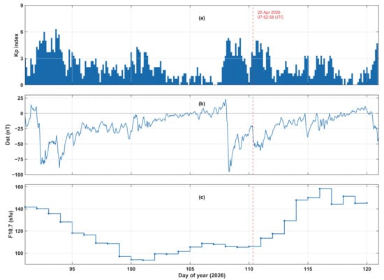
The Kp index remained below five during most of the days preceding the earthquake, with a moderate enhancement (Kp ≈ 4–5) on day-of-year (DOY) 107–109 (17–19 April) coinciding with a Dst minimum of approximately −95 nT on DOY 108 (18 April), indicative of a moderate geomagnetic storm (Figure 3). At the earthquake occurrence (DOY 110.33, 07:52:58 UTC on 20 April), the ionosphere was in the storm recovery phase, with Dst recovered to approximately −20 to −30 nT and Kp at moderate levels (Kp ≈ 3–4). These conditions were well below those typically associated with strong storm-time traveling ionospheric-disturbance activity (Kp ≥ 6–7; Dst ≤ −100 nT).
Figure 3.
Solar and geomagnetic conditions during DOY 91–120 of 2026: (a) 3-hourly Kp index, (b) hourly Dst index, and (c) daily F10.7 cm solar radio flux. The red dashed vertical line marks the 20 April 2026 Mw 7.4 earthquake (DOY 110; 07:52:58 UTC).
Solar activity was likewise low, with F10.7 increasing gradually from a solar-minimum-like value of ~90 sfu around DOY 100–102 to ~105–110 sfu at the time of the earthquake. The Savitzky–Golay detrending removed variability on timescales longer than approximately 30 min, thereby suppressing residual contributions from the decaying geomagnetic disturbance to the background TEC trend before band-pass filtering. Consequently, the short-period (2–10 min) perturbations analyzed here are unlikely to reflect concurrent geomagnetic activity; nonetheless, transient short-period disturbances associated with impulsive substorm or storm-sudden-commencement activity cannot be entirely excluded during the recovery phase of a geomagnetic disturbance, and a minor residual contribution from space-weather forcing cannot be ruled out on this basis alone [29].
3.2. Station–Satellite Geometry and IPP Distribution
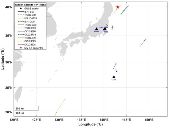
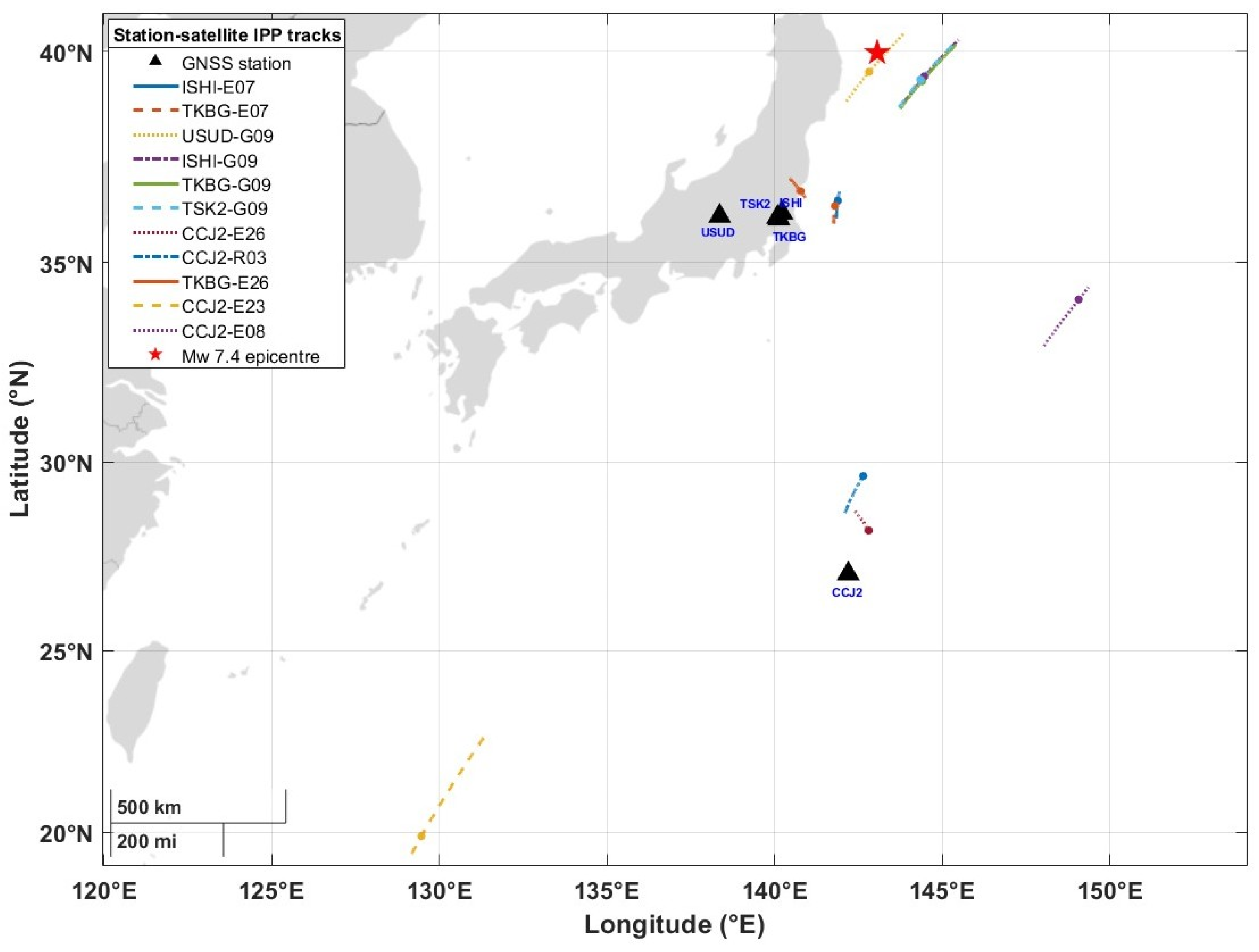
The 11 station–satellite links sampled IPPs over a wide geographic area, extended from the near-source region to more than 2500 km from the epicentre (Figure 4). At the selected disturbance arrivals, the IPPs extended from 19.89° N to 39.53° N and from 129.47° E to 149.06° E, with epicentral distances ranging from 52.84 km (USUD-G09) to 2581.26 km (CCJ2-E23).
Figure 4.
Ground tracks of the ionospheric pierce points (IPPs) for the selected GNSS station–satellite links. Black triangles mark GNSS receiver locations, coloured and patterned lines show the IPP trajectories, and the red star indicates the earthquake epicentre. Coloured points identify the IPP positions associated with the associated disturbance arrivals.
The four G09 links provided the principal near-field sampling. USUD-G09 had an IPP located 52.84 km from the epicentre at 39.53° N, 142.82° E, while TSK2-G09, ISHI-G09, and TKBG-G09 sampled a compact cluster of IPPs east of the epicentre, at epicentral distances of 130.28, 134.41, and 135.44 km, respectively. Together, these links defined a concentrated near-field sampling region extending approximately 53–135 km from the epicentre. The E07 and E26 links extended the spatial sampling into an intermediate-distance region south of the epicentre. ISHI-E07, TKBG-E07, and TKBG-E26 sampled IPPs at epicentral distances of 399.10, 414.37, and 411.55 km, respectively, with IPP locations distributed between 36.38 and 36.73° N and between 140.78 and 141.88° E. These observations formed a relatively compact intermediate-distance group approximately 400–415 km from the epicentre.
The CCJ2 observations further extended the spatial sampling into the far field. CCJ2-R03 and CCJ2-E26 sampled IPPs at epicentral distances of 1150.77 and 1308.27 km, respectively, while CCJ2-E23 extended the detected spatial range to 2581.26 km. Thus, the station–satellite configuration provided IPP sampling across near-field, intermediate-distance, and far-field regions, with substantial variation in both geographic position and epicentral distance.
Despite this spatial progression, the associated perturbation arrival sequence was not strictly monotonic with epicentral distance. In particular, CCJ2-E23, despite having the largest epicentral distance of 2581.26 km, yielded an earlier selected arrival than CCJ2-R03 and CCJ2-E26. Similarly, USUD-G09, despite having the shortest IPP–epicentre distance of 52.84 km, did not exhibit the earliest disturbance arrival. The absence of a monotonic relationship between arrival time and IPP–epicentre distance indicates that radial distance alone cannot explain the observed arrival sequence. Instead, the timing appears to depend on the direction of propagation and the spatial distribution of the sampled IPPs, motivating the directional hodochrone analysis employed.
3.3. Detrended TEC Waveforms and N-Shaped Signatures
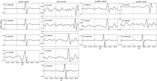
All analyzed station–satellite links exhibit a clear bipolar, N-shaped dTEC perturbation following the earthquake origin time, consistent with the passage of a transient atmospheric disturbance through the respective IPPs (Figure 5). The characteristic (peak) dTEC disturbance time occurs 8–17 min after the origin time across the network. Peak-to-peak dTEC amplitudes vary by more than one order of magnitude, ranging from approximately 0.05–0.1 TECU for the more distant, lower-elevation CCJ2 Galileo/GLONASS links (E07, E08, E23, E26, and R03) to approximately 1.0–1.2 TECU for the near-field, high-elevation GPS G09 links at TKBG, TSK2, ISHI, and USUD. This amplitude contrast likely reflects the combined influence of propagation-distance-dependent attenuation and differences in receiver–satellite viewing geometry. Although lower-elevation links provide longer slant paths through the ionosphere and can enhance the observed slant-TEC response to spatially structured perturbations, this geometric effect does not appear to compensate for the substantially weaker signals observed on the more distant CCJ2 links.
Figure 5.
Detrended and band-pass filtered dTEC time series for each station–satellite links, grouped by azimuthal sector: (a) southeast (138.93°); (b) south (181.09°); (c) south–southwest (195.80); (d) southwest (214.09). Each panel is labeled with the contributing GNSS station and satellite pseudo-random number (PRN; G = GPS, E = Galileo, R = GLONASS). The vertical red dashed line marks the earthquake origin time (07:52:58 UTC).
Several links, including TKBG-E07 and ISHI-E07, also exhibit a secondary, lower-amplitude oscillatory tail following the principal N-shaped pulse. The presence of this trailing structure suggests that the disturbance may comprise a short-wave train rather than a single isolated pulse, consistent with the oscillatory signatures commonly reported for shock-acoustic coseismic ionospheric disturbances [12,30].
3.4. Hodochrone Analysis and Propagation Velocities
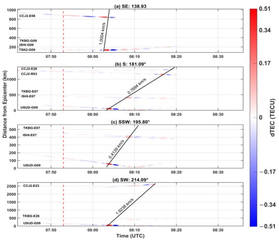
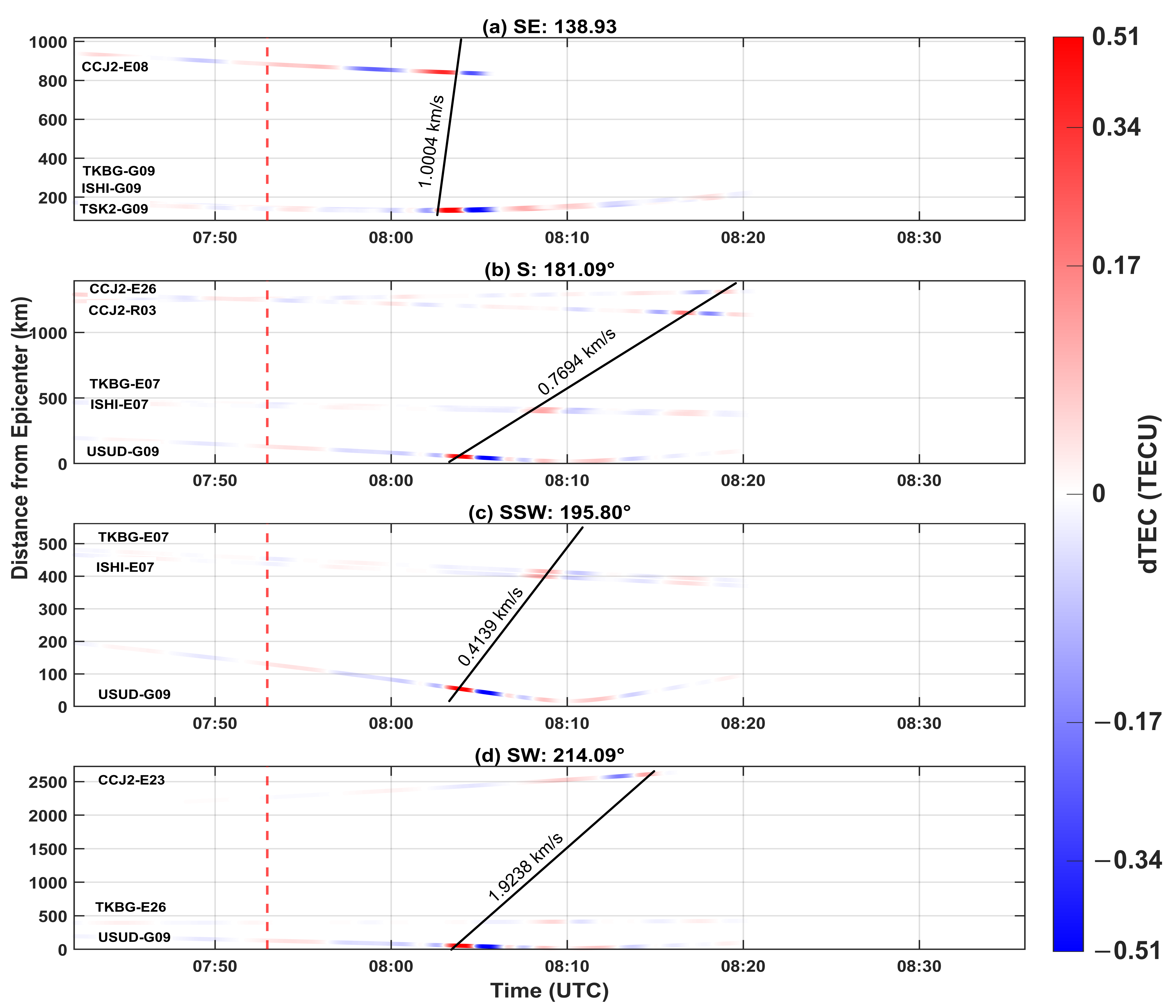
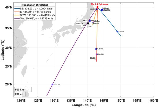
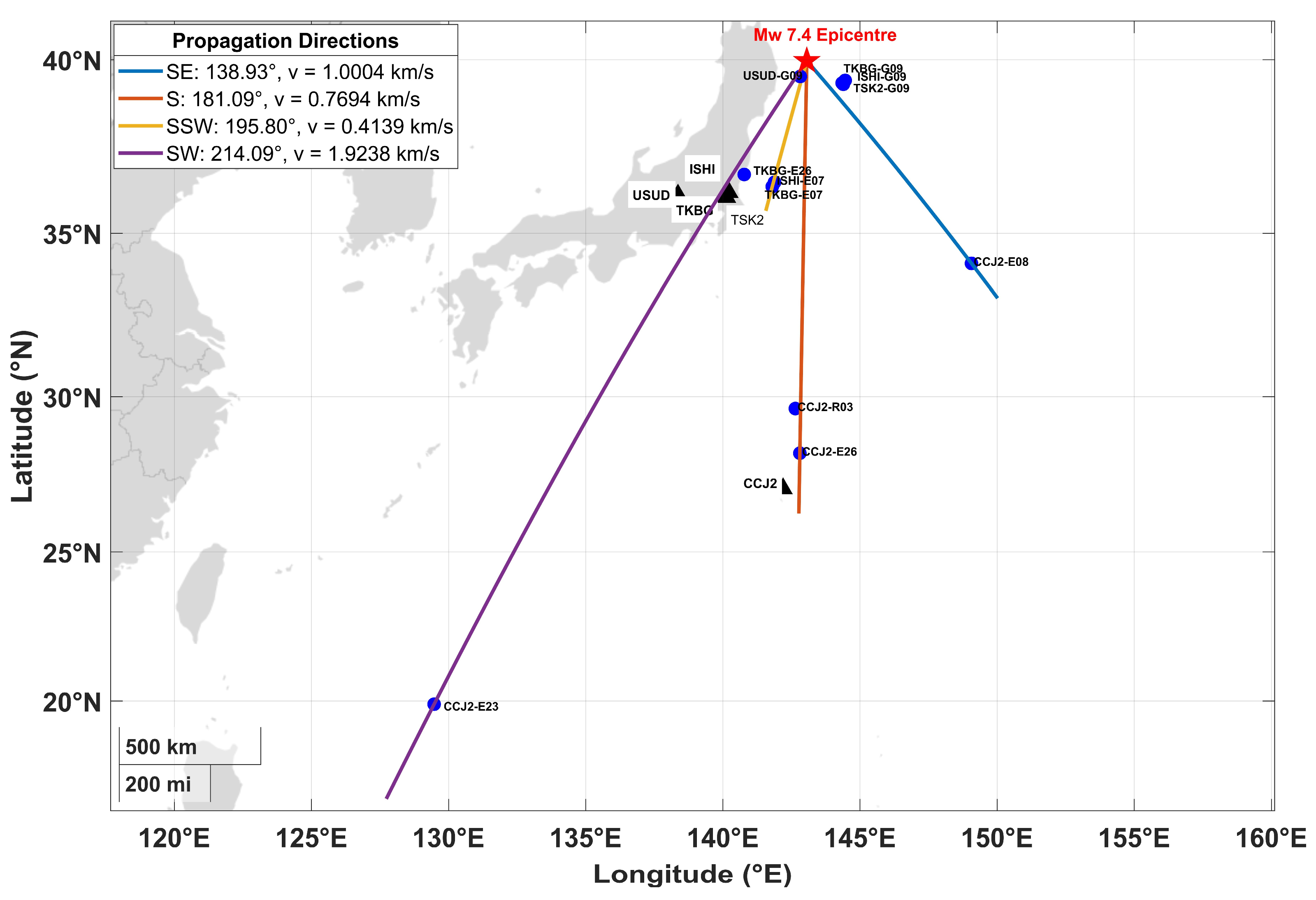
Linear fits to the peak-time–IPP-distance relationships within the four azimuthal sectors yield apparent horizontal propagation velocities, computed from IPP ground-track distance under the 350 km thin-shell approximation without correction for wave incidence angle, of 1.00 km s−1 (SE, 138.9°), 0.77 km s−1 (S, 181.1°), 0.41 km s−1 (SSW, 195.8°), and 1.92 km s−1 (SW, 214.1°) (Figure 6 and Figure 7; Table 3). With the exception of the SW sector, these velocities are substantially lower than the 2.9–4.2 km s−1 values commonly reported for Rayleigh-wave-driven ionospheric disturbances [12,30,31], and are more consistent with the approximately 0.6–1.5 km s−1 velocities reported for directly excited, vertically propagating shock-acoustic disturbances [9,12]. Following established terminology, acoustic disturbances refer to coseismic atmospheric waves propagating near the ambient sound speed, whereas shock-acoustic disturbances refer to higher-amplitude near-field responses in which nonlinear steepening may occur during propagation following coseismic vertical displacement. The apparent velocities obtained here fall within ranges previously attributed to shock-acoustic disturbances. However, the present observations provide no independent evidence of nonlinear wave behaviour, such as wavefront steepening, amplitude-dependent dispersion, or diagnostic near-field waveform characteristics. Accordingly, the term shock-acoustic is used here on the basis of consistency with previously reported propagation velocities and should not be interpreted as direct evidence of nonlinear wave propagation. The SSW sector exhibits the lowest apparent velocity (0.41 km s−1) below the range typically reported for directly excited acoustic disturbances. This unusually low value should, however, be interpreted cautiously because the sector is constrained by only three IPP tracks spanning a relatively limited distance range of approximately 20–520 km (Table 3), making the fitted slope particularly sensitive to individual arrival-time uncertainties and IPP geometry.
Figure 6.
Distance–time (hodochrone) representation of the dTEC perturbations shown in Figure 5, plotted as a function of IPP distance from the epicentre and time (UTC), for the (a) SE, (b) S, (c) SSW and (d) SW azimuthal sectors. Colour indicates dTEC amplitude. Diagonal black lines and annotated values show the linear hodochrone fit and corresponding apparent propagation velocity for each sector. The vertical red dashed line marks the earthquake origin time.
Figure 7.
Geographic representation of the four azimuthal propagation directions, overlaid on the IPP/station geometry relative to the Mw 7.4 epicentre (red star). Blue circles indicate IPP locations associated with the identified disturbance arrivals, while black triangles denote GNSS stations.
Table 3.
Summary of azimuthal-sector hodochrone analysis.
The SW-sector velocity of 1.92 km s−1 occupies an intermediate range between velocities commonly associated with directly excited acoustic and Rayleigh-wave-driven ionospheric disturbances. It is comparable to the slower secondary branch of 1.1–1.6 km s−1 reported over Japan following the 2025 Mw 8.8 Kamchatka earthquake [31], as well as to the approximately 2 km s−1 ionospheric-disturbance velocity observed over Siberia for the same event, which was approximately 1.5 times lower than the co-located Rayleigh-wave velocity [32]. The substantially lower magnitude of the Mw 7.4 Miyako earthquake relative to the Mw 8.8 Kamchatka event implies weaker seismic excitation and potentially weaker surface-wave forcing at ionospheric altitudes. The intermediate velocity observed in the SW sector may therefore reflects a weaker or less coherent Rayleigh-wave-driven response, a relatively greater contribution from directly excited acoustic disturbances, or a combination of propagation characteristics and receiver–satellite sampling geometry.
3.5. Ionosonde Multiple Cusp Signatures
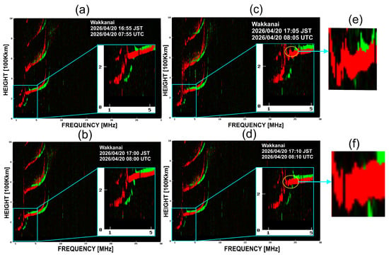
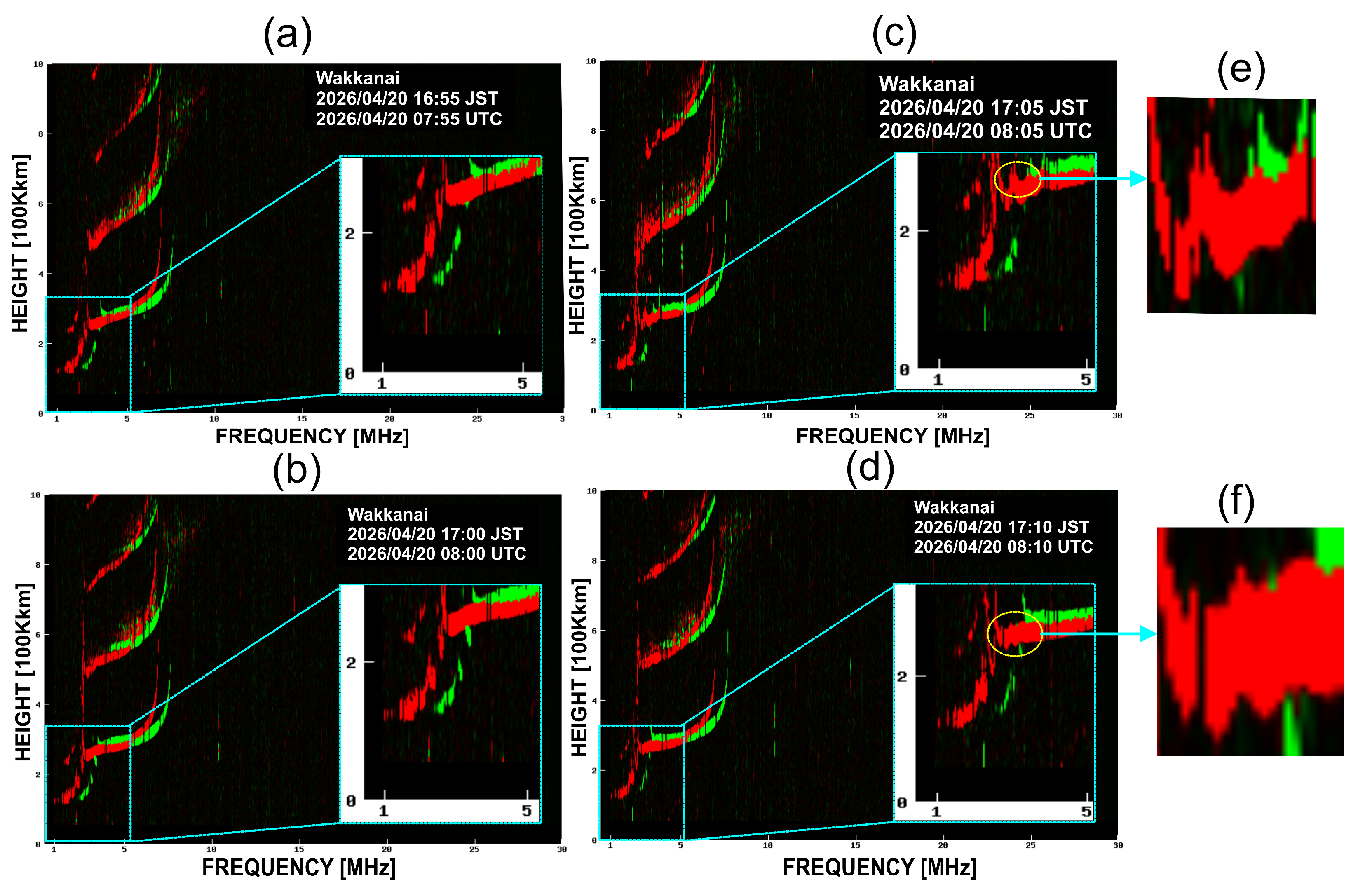
MCS were identified in ionograms from all three ionosonde stations, with onset times spanning approximately 12–17 min after the earthquake origin time of 07:52:58 UTC. The timing and morphology of the signatures varied systematically among the stations. At Wakkanai, located approximately 626 km from the epicentre and at the highest magnetic latitude of the three stations, successive 5 min ionograms show a progressive evolution of the F-region trace. The profile remains largely undisturbed at 07:55 and 08:00 UTC, develops a faint cusp-like deformation by 08:05 UTC, and exhibits a well-defined, sharp-edged cusp at 08:10 UTC (Figure 8). The MCS therefore becomes identifiable between 08:05 and 08:10 UTC, corresponding to approximately 12–17 min after the earthquake origin time.
Figure 8.
Sequence of ionograms from Wakkanai on 20 April 2026: (a) 07:55 UTC; (b) 08:00 UTC; (c) 08:05 UTC, showing the faint emergence of the MCS; (d) 08:10 UTC, showing the clearly developed MCS; (e) enlarged view of the MCS highlighted in (c); and (f) enlarged view of the MCS highlighted in (d). The insets in (a–d) show enlarged views of the F-region trace.
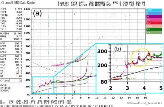
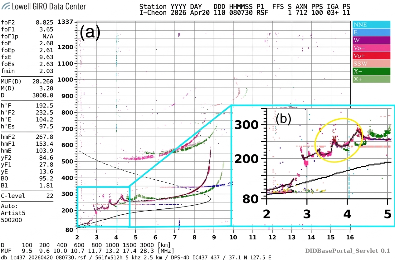
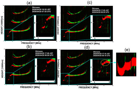
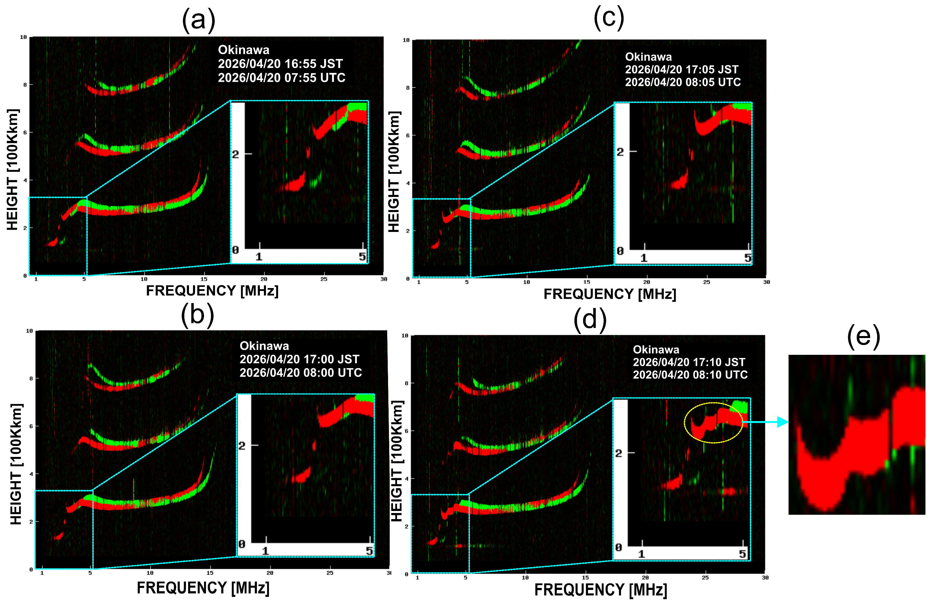
Icheon, located approximately 1451 km from the epicentre, provides an ionogram at 08:07:30 UTC showing a distinct step-like deformation of the F-region trace at virtual heights of approximately 200–300 km (Figure 9). This feature occurs approximately 14.5 min after the earthquake origin time and provides independent ionosonde evidence of a transient ionospheric disturbance at an intermediate epicentral distance. Farther from the source, Okinawa is located approximately 2121 km from the epicentre and at the lowest magnetic latitude of the three stations. Its F-region trace remains comparatively smooth through 08:05 UTC, before developing a broader and less sharply defined multi-cusp deformation by 08:10 UTC (Figure 10), corresponding to approximately 17 min after the earthquake origin time. Despite its substantially greater epicentral distance, the Okinawa MCS therefore occurs within a temporal window comparable to those observed at Wakkanai and Icheon.
Figure 9.
Ionogram from Icheon (Republic of Korea; DIDBase station code IC437) at 08:07:30 UTC on 20 April 2026. (a) Full ionogram showing the observed ionospheric traces, with the coloured dots representing the ionogram trace data; (b) enlarged view of the F-region trace, with the yellow circle highlighting the region containing the identified step-like MCS deformation.
Figure 10.
Sequence of ionograms from Okinawa on 20 April 2026: (a) 07:55 UTC; (b) 08:00 UTC; (c) 08:05 UTC; (d) 08:10 UTC, showing the identified MCS deformation highlighted by the yellow circle; and (e) enlarged view of the MCS deformation highlighted in (d). The insets in (a–d) show enlarged views of the F-region trace.
The morphology of the MCS also varies among the three stations. Wakkanai exhibits the sharpest and most clearly defined cusp, Icheon shows an intermediate step-like deformation, whereas Okinawa displays a broader and more subdued structure. This qualitative progression from a sharper to a less distinct signature toward lower magnetic latitude is consistent with the expected dependence of acoustic-wave-to-plasma coupling on magnetic-field geometry [33]. However, because the stations differ simultaneously in epicentral distance, magnetic latitude, ionospheric state, and observational sampling, the relative contribution of magnetic-field geometry cannot be isolated from these observations alone. The ionosonde results therefore provide complementary evidence for a spatially extended coseismic ionospheric response, while the observed differences in MCS morphology should be interpreted as qualitative rather than as a direct quantitative measure of coupling efficiency.
4. Discussion
The apparent velocities estimated for the Miyako earthquake range from 0.4139 to 1.9238 km s−1 across the SE cluster and the three nested SSW solutions, all of which are below the 2.9–4.2 km s−1 range reported for Rayleigh-wave-driven acoustic coupling in comparable studies [12,30,31]. The lowest apparent velocity (0.4139 km s−1), obtained from the SSW short-baseline solution spanning 361.5 km, and the SE population value (1.0004 km s−1) fall within or close to the 0.6–1.5 km s−1 range reported for directly and vertically excited shock-acoustic waves [9,12]. The SSW value of 0.4139 km s−1 is below the 1.1–1.6 km s−1 secondary branch reported for the 2025 Kamchatka earthquake over Japan by Barad et al. [31]. In contrast, the highest value of 1.9238 km s−1, obtained for the SW direction, is comparable to the approximately 2 km s−1 apparent ionospheric-disturbance velocity reported by Oinats et al. [32] for the same event over Siberia. The latter was approximately 1.5 times slower than the co-located Rayleigh wave. Collectively, these findings suggest that the Miyako disturbances are more consistent with apparent propagation velocities lower than typical Rayleigh-wave-associated CID velocities than with a dominant Rayleigh-wave-driven coupling mechanism.
Importantly, the apparent velocity systematically increases with the spatial span of the fitted SSW solution, from 0.4139 to 0.7694 and 1.9238 km s−1 as the span increases from 361.5 to 1255.4 and 2528.4 km, respectively. This behaviour is consistent with the distance-dependent characteristics reported for the 2025 Kamchatka disturbance over southwestern Japan. Barad et al. [31] attributed the emergence of faster wave velocities at greater distances to the increasing detectability of a Rayleigh-wave component relative to a slower near-field acoustic component, rather than to actual acceleration of the disturbance. A similar interpretation may therefore apply to Miyako observation, with the progressively larger apparent velocities reflecting changes in the relative contribution and detectability of different disturbance components across the network rather than a change in the intrinsic propagation speed of a single wave. The detection of ionospheric perturbations associated with an event of comparable magnitude (Mw 7.4) in the 2019 Indonesian earthquake using combined GPS and VLF measurements [34] further demonstrates that CIDs can be detected reliably within this magnitude range, even where a distinct Rayleigh-wave component cannot be resolved.
The noticeable azimuthal contrast in waveform amplitude and apparent propagation velocity provide further evidence that the coseismic ionospheric response is spatially heterogeneous and directionally dependent. Such anisotropy is likely to arise from the interaction of several processes, including the seismic source radiation pattern and rupture geometry, the orientation of the GNSS line of sight relative to the local geomagnetic field, which controls the efficiency of acoustic-to-TEC coupling [9,26], and variations in thermospheric winds and composition along the propagation path. The semi-analytic modeling of earthquake-generated acoustic-gravity waves shows that focal mechanism alone can produce markedly different directional energy distributions, providing a plausible physical basis for part of the observed azimuthal contrast, although this mechanism was not directly tested with the present dataset [27]. Comparable azimuthal variability has been documented following the 2015 Gorkha, 2020 Jamaica, and 2022 Mexico earthquakes [7,8,21]. In particular, Li et al. [21] demonstrated that the azimuthal dependence of GNSS-derived disturbances following the 2022 Mexico earthquake resulted from the combined effects of source radiation, atmospheric propagation, geomagnetic-field orientation, and line-of-sight sensitivity. Spatially resolved ionospheric observations can also retain information about fault-slip and rupture geometry [6], while far-field CID distributions may be further modified by underlying geological structure [35]. Thus, the observed directional differences in amplitude and apparent velocity should not be interpreted as evidence for a single propagation mechanism. Rather, they reflect the coupled influence of source characteristics, atmospheric and ionospheric propagation, geomagnetic geometry, and spatially varying conditions along the propagation path.
The Multiple Cusp Signatures (MCS) observed across the ionosonde network provide an additional perspective on the propagation of the disturbance. The qualitative variation in MCS sharpness, from the sharp and well-developed signature at Wakkanai through the intermediate step-like deformation at Icheon to the broader and more subdued structure at Okinawa, is consistent with the mechanism proposed by Maruyama et al. [33], whereby the efficiency of ion–neutral coupling between an upward-propagating acoustic wave and the ambient magnetic field increases with geomagnetic inclination. Under this framework, MCS are expected to be more evident at higher magnetic latitudes, providing a plausible explanation for the observed latitudinal variation in signature strength.
The timing of the ionosonde signatures is also broadly compatible with the GNSS-derived disturbances. The 12–17 min MCS onset window recorded across the ionosonde network falls within the 10.07–24.62 min range of GNSS-derived peak-time delays and matches the delay range associated with the SSW short-baseline and extended solutions (940–1477 s). This temporal correspondence supports a common causal origin. However, the ionosonde observations provide only a relatively coarse spatial constraint on the disturbance propagation. At the apparent velocities inferred from GNSS (0.41–1.92 km s−1), a disturbance would traverse approximately 120–570 km between successive ionograms, which is several times larger than the spatial separation required to discriminate robustly among SSW solutions. Similar limitations have been recognized by Haralambous et al. [9] and Paul et al. [30] for their respective studies. Consequently, the ionosonde observations should be interpreted as broadly consistent with the GNSS-derived timing and propagation characteristics rather than as an independent quantitative constraint on GNSS velocity estimates.
Ultimately, the Miyako case study demonstrates that combined GNSS-TEC and ionosonde monitoring can successfully resolve short-period and directionally structured coseismic ionospheric disturbances associated with moderate interplate earthquakes. The observations extend the range of earthquake magnitudes for which such ionospheric signatures can be characterized in detail and, importantly, show that moderate earthquakes can generate disturbances with apparent propagation velocities lower than typical Rayleigh-wave-associated CID velocities, and with strongly direction-dependent behaviour. Given the higher recurrence rate of Mw 7–7.5 earthquakes compared with great earthquakes (Mw ≥ 8), improved characterization of their ionospheric signatures is relevant to the continued development of GNSS- and ionosonde-based earthquake early-warning concepts [15,17].
5. Conclusions
High-rate GNSS-TEC and ionosonde observations of the 20 April 2026 Mw 7.4 Miyako, Japan earthquake reveal clear coseismic ionospheric disturbances across a regional receiver network spanning approximately 500–2100 km in epicentral distance, while the ionospheric pierce points sampled by the corresponding station–satellite links extended from approximately 53 to 2581 km from the epicentre, reflecting oblique satellite-viewing geometry. Detrended TEC time series exhibited characteristic N-shaped perturbations with peak disturbance times of 8–17 min after the earthquake origin time and peak-to-peak amplitudes of approximately 0.05–1.2 TECU, largest on near-field, high-elevation GPS links. Hodochrone analysis yields apparent propagation velocities of 0.41–1.92 km s−1 across the southeast, south, south–southwest, and southwest sectors, respectively, markedly slower than the 2.9–4.2 km s−1 velocity range widely reported for Rayleigh-wave-associated ionospheric disturbances following larger earthquakes, and instead consistent with directly excited shock-acoustic propagation characterized by pronounced azimuthal anisotropy. Ionosonde observations at Wakkanai, Icheon and Okinawa confirm the presence of Multiple Cusp Signatures 12–17 min after the earthquake, with cusp sharpness decreasing from the highest to the lowest magnetic latitude station, qualitatively consistent with inclination-dependent acoustic-to-plasma coupling efficiency. Background Kp (~3–4), Dst (~−20 to −30 nT) and F10.7 (~105–110 sfu) indices indicate that the ionosphere was in the recovery phase of a moderate geomagnetic disturbance but not under active storm conditions at the time of the earthquake, supporting a seismogenic rather than space-weather origin for the reported perturbations. These findings extend characterization of coseismic ionospheric disturbances associated with Mw 7–7.5 earthquakes by demonstrating pronounced azimuthal anisotropy and apparent propagation velocities substantially below those typically associated with Rayleigh-wave-driven ionospheric responses.
Author Contributions
Conceptualization, H.H.; methodology, M.M., H.H. and T.B.; software, M.M.; validation, M.M., H.H. and T.B.; formal analysis, H.H., M.M. and T.B.; data curation, M.M. and T.B.; writing, original draft preparation, M.M.; writing—review and editing, M.M., H.H. and T.B.; visualization, M.M. and T.B.; supervision, H.H. All authors have read and agreed to the published version of the manuscript.
Funding
This research received no external funding.
Data Availability Statement
The processed GNSS-TEC data used in this study are publicly available through Zenodo at https://doi.org/10.5281/zenodo.22703232 (accessed on 11 September 2026). The 1 Hz GNSS observations used to derive slant total electron content were obtained from NASA’s Crustal Dynamics Data Information System (CDDIS), including the CDDIS GNSS high-rate archive. Icheon ionograms were obtained from the Global Ionosphere Radio Observatory Digital Ionogram Database (DIDBase). Wakkanai and Okinawa ionograms were obtained from the National Institute of Information and Communications Technology (NICT), Japan, through the World Data Center for Ionosphere and Space Weather and the NICT ionosonde archive. Solar and geomagnetic indices, including Kp, Dst, and F10.7, were obtained from NASA’s OMNIWeb database and can be accessed through the OMNIWeb Data Explorer. Earthquake source parameters and ShakeMap products were obtained from the USGS ANSS Comprehensive Earthquake Catalog and the USGS ShakeMap archive, respectively. All datasets used in this study are publicly accessible through their respective repositories.
Acknowledgments
We acknowledge the Global Ionosphere Radio Observatory for providing the ionosonde data from Icheon, Republic of Korea. Ionosonde observations from Wakkanai and Okinawa, Japan, were obtained from the National Institute of Information and Communications Technology (NICT), Japan. GNSS observations were obtained from NASA’s Crustal Dynamics Data Information System (CDDIS). Solar and geomagnetic indices were obtained from the OMNI database through the NASA Goddard Space Flight Center (GSFC) Space Physics Data Facility (SPDF) OMNIWeb interface.
Conflicts of Interest
Author Trisani Biswas is employed by the company GeoImaging Ltd. The remaining authors declare that the research was conducted in the absence of any commercial or financial relationships that could be construed as a potential conflict of interest.
Abbreviations
The following abbreviations are used in this manuscript:
| CID | Coseismic ionospheric disturbance |
| CMT | Centroid Moment Tensor (as in the Global CMT project) |
| DIDBase | Digital Ionogram Database |
| DPS-4D | Digisonde Portable Sounder (ionosonde model) |
| Dst | Disturbance storm-time index (geomagnetic) |
| dTEC | Detrended/differential Total Electron Content |
| F10.7 | Solar radio flux at 10.7 cm wavelength |
| foF2 | F2-layer critical frequency |
| GEONET | GNSS Earth Observation Network System (Japan) |
| GFZ | GeoForschungsZentrum Potsdam (German Research Centre for Geosciences) |
| GIRO | Global Ionospheric Radio Observatory |
| GNSS | Global Navigation Satellite System |
| GSI | Geospatial Information Authority of Japan |
| hmF2 | Height of the F2-layer peak electron density |
| IGRF | International Geomagnetic Reference Field |
| IGS | International GNSS Service |
| IPP | Ionospheric pierce point |
| JMA | Japan Meteorological Agency |
| Kp | Planetary K index (geomagnetic) |
| L1, L2, L5 | GNSS carrier-phase frequency bands (~1575, ~1227 and ~1176 MHz, respectively) |
| LAI | Lithosphere–atmosphere–ionosphere (coupling) |
| MCS | Multiple Cusp Signatures |
| MMI | Modified Mercalli Intensity |
| Mw | Moment magnitude |
| NICT | National Institute of Information and Communications Technology (Japan) |
References
- Astafyeva, E.; Heki, K.; Kiryushkin, V.; Afraimovich, E.; Shalimov, S. Two-mode long-distance propagation of coseismic ionosphere disturbances. J. Geophys. Res. Space Phys. 2009, 114, A10307. [Google Scholar] [CrossRef] [Scilit]
- Liu, H.; Ding, F.; Zhao, B.; Li, J.; Hu, L.; Wan, W.; Ning, B. Ionospheric response following the Mw 7.8 Gorkha earthquake on 25 April 2015. J. Geophys. Res. Space Phys. 2017, 122, 6495–6507. [Google Scholar] [CrossRef] [Scilit]
- Pal, S.K.; Nanda, K.; Sarkar, S.; Potirakis, S.M.; Hayakawa, M.; Sasmal, S. Comparative statistical detection of ionospheric GPS-TEC anomalies associated with the 2021 Haiti and 2022 Cyprus earthquakes. Geosciences 2026, 16, 129. [Google Scholar] [CrossRef] [Scilit]
- Liu, J.Y.; Tsai, H.F.; Lin, C.H.; Kamogawa, M.; Chen, Y.I.; Lin, C.H.; Huang, B.S.; Yu, S.B.; Yeh, Y.H. Coseismic ionospheric disturbances triggered by the Chi-Chi earthquake. J. Geophys. Res. 2010, 115, A08303. [Google Scholar] [CrossRef] [Scilit]
- Liu, J.; Chen, C.; Lin, C.; Tsai, H.; Chen, C.; Kamogawa, M. Ionospheric disturbances triggered by the 11 March 2011 M9.0 Tohoku earthquake. J. Geophys. Res. 2011, 116, A06319. [Google Scholar] [CrossRef] [Scilit]
- Astafyeva, E.; Lognonné, P.; Rolland, L. First ionospheric images of the seismic fault slip on the example of the Tohoku-oki earthquake. Geophys. Res. Lett. 2011, 38, L22104. [Google Scholar] [CrossRef] [Scilit]
- Tulasi Ram, S.; Sunil, P.S.; Ravi Kumar, M.; Su, S.-Y.; Tsai, L.C.; Liu, C.H. Coseismic traveling ionospheric disturbances during the Mw 7.8 Gorkha, Nepal earthquake on 25 April 2015 from ground and spaceborne observations. J. Geophys. Res. Space Phys. 2017, 22, 10669–10685. [Google Scholar] [CrossRef] [Scilit]
- Chai, Y.; Jin, S. Two-azimuth co-seismic ionospheric disturbances following the 2020 Jamaica earthquake from GPS observations. J. Geophys. Res. Space Phys. 2021, 126, e2020JA028995. [Google Scholar] [CrossRef] [Scilit]
- Haralambous, H.; Guerra, M.; Chum, J.; Verhulst, T.G.W.; Barta, V.; Altadill, D.; Cesaroni, C.; Galkin, I.; Márta, K.; Mielich, J.; et al. Multi-instrument observations of various ionospheric disturbances caused by the 6 February 2023 Turkey earthquake. J. Geophys. Res. Space Phys. 2023, 128, e2023JA031691. [Google Scholar] [CrossRef] [Scilit]
- Alfonsi, L.; Cesaroni, C.; Hernández-Pajares, M.; Astafyeva, E.; Bufféral, S.; Elias, P.; Belehaki, A.; Ioanna, T.; Yang, H.; Guerra, M. Ionospheric response to the 2020 Samos earthquake and tsunami. Earth Planets Space 2024, 76, 13. [Google Scholar] [CrossRef] [Scilit]
- Chen, Y.; Wang, K.; Li, W.; Liu, X. The coseismic ionospheric disturbance during 2023 Turkey double earthquake monitored by GNSS observations. IEEE J. Sel. Top. Appl. Earth Obs. Remote Sens. 2025, 18, 18830–18842. [Google Scholar] [CrossRef] [Scilit]
- Biswas, T.; Moses, M.; Haralambous, H.; Mostafa, M.G. Insights into seismic-induced ionospheric perturbation following the 2025 Myanmar earthquake. J. Geophys. Res. Space Phys. 2025, 130, e2025JA034243. [Google Scholar] [CrossRef] [Scilit]
- Bagiya, M.S.; Sunil, A.S.; Rolland, L.; Nayak, S.; Ponraj, M.; Thomas, D.; Ramesh, D.S. Mapping the impact of non-tectonic forcing mechanisms on GNSS measured coseismic ionospheric perturbations. Sci. Rep. 2019, 9, 18640. [Google Scholar] [CrossRef] [Scilit]
- Yang, Y.; Komanduru, A.; Garrison, J. Detection of atmospheric-ionospheric disturbances in TEC time series from large GNSS networks using wavelet coherence. IEEE J. Sel. Top. Appl. Earth Obs. Remote Sens. 2023, 16, 5154–5172. [Google Scholar] [CrossRef] [Scilit]
- Brissaud, Q.; Astafyeva, E. Near-real-time detection of co-seismic ionospheric disturbances using machine learning. Geophys. J. Int. 2022, 230, 2117–2130. [Google Scholar] [CrossRef] [Scilit]
- Heki, K.; Bagiya, M.; Takasaka, Y. Slow fault slip signatures in coseismic ionospheric disturbances. Geophys. Res. Lett. 2022, 49, e2022GL101064. [Google Scholar] [CrossRef] [Scilit]
- Wüst, S.; Guerra, M.; Chum, J.; Gasque, L. Using atmospheric waves for the detection and early warning of natural hazards: A review combining results from the neutral atmosphere and the ionosphere. Surv. Geophys. 2026. [Google Scholar] [CrossRef] [Scilit]
- Tsugawa, T.; Saito, A.; Otsuka, Y.; Nishioka, M.; Maruyama, T.; Kato, H.; Nagatsuma, T.; Murata, K.T. Ionospheric disturbances detected by GPS total electron content observation after the 2011 off the Pacific coast of Tohoku Earthquake. Earth Planets Space 2011, 63, 66. [Google Scholar] [CrossRef] [Scilit]
- Ruan, Q.; Yuan, X.; Liu, H.; Ge, S. Study on co-seismic ionospheric disturbance of Alaska earthquake on July 29, 2021 based on GPS TEC. Sci. Rep. 2023, 13, 10679. [Google Scholar] [CrossRef] [Scilit]
- Cahyadi, M.N.; Muslim, B.; Pratomo, D.; Anjasmara, I.M.; Arisa, D.; Rahayu, R.W.; Hariyanto, I.H.; Jin, S.; Muafiry, I.N. Co-seismic ionospheric disturbances following the 2016 West Sumatra and 2018 Palu earthquakes from GPS and GLONASS measurements. Remote Sens. 2022, 14, 401. [Google Scholar] [CrossRef] [Scilit]
- Li, L.; Jin, S.; Chai, Y. Co-seismic ionospheric disturbances characteristics in different azimuths following the 2022 Mexico earthquake from GNSS observations. GPS Solut. 2023, 28, 23. [Google Scholar] [CrossRef] [Scilit]
- Chen, C.H.; Saito, A.; Lin, C.H.; Liu, J.Y.; Tsai, H.F.; Tsugawa, T.; Otsuka, Y.; Nishioka, M.; Matsumura, M. Long-distance propagation of ionospheric disturbance generated by the 2011 off the Pacific coast of Tohoku Earthquake. Earth Planets Space 2011, 63, 881–884. [Google Scholar] [CrossRef] [Scilit]
- Zhang, J.; Gao, Y.; Hu, H.; Chen, C.-H.; Zhang, X. Acoustic-gravity wave driven traveling ionospheric disturbances: Analytical modeling and application to 2025 Kamchatka earthquake GNSS data. Earth Planet. Sci. Lett. 2026, 693, 120299. [Google Scholar] [CrossRef] [Scilit]
- Chen, C.-H.; Zhang, S.; Gao, Y.; Chen, L.; Li, J.; Zhang, X.; Chen, Y.-C.; Tang, C.-C.; Hu, J.; Liu, H.; et al. Doppler frequency shifts associated with the 29 July 2025 M8.8 Kamchatka earthquake in southwest China. J. Geophys. Res. Space Phys. 2026, 131, e2025JA034917. [Google Scholar] [CrossRef] [Scilit]
- Zhivetiev, I. Tec-Suite Documentation (Release v0.7.8) [Software Documentation]. 2020. Available online: https://tec-suite.readthedocs.io/_/downloads/en/latest/pdf/ (accessed on 2 July 2026).
- Rolland, L.M.; Lognonné, P.; Munekane, H. Detection and modeling of Rayleigh wave induced patterns in the ionosphere. J. Geophys. Res. Space Phys. 2011, 116, A05320. [Google Scholar] [CrossRef] [Scilit]
- Li, T.; Gao, Y.; Chen, C.-H.; Sun, Y.-Y.; Zhang, X.; Chum, J.; Zhou, G.; Wen, J.; Chen, X. Simulation of acoustic-gravity waves generated by an earthquake and explanation of the ionospheric disturbance observed during 2023 M 7.7 Turkey earthquake. J. Geophys. Res. Space Phys. 2025, 130, e2025JA033711. [Google Scholar] [CrossRef] [Scilit]
- Maruyama, T.; Tsugawa, T.; Kato, H.; Ishii, M.; Nishioka, M. Rayleigh wave signature in ionograms induced by strong earthquakes. J. Geophys. Res. 2012, 117, A08306. [Google Scholar] [CrossRef] [Scilit]
- Hajra, S.; Dashora, N.; Ivan, J.S. Global observations of the short-term disturbances in the geomagnetic field and induced currents during the supersubstorms events of solar cycle 24. Space Weather 2023, 21, e2022SW003355. [Google Scholar] [CrossRef] [Scilit]
- Paul, K.S.; Biswas, T.; Haralambous, H.; Moses, M. Ionospheric disturbances induced by the 29 July 2025 Kuril–Kamchatka earthquake: Multi-instrument observations and analysis. J. Geophys. Res. Space Phys. 2026, 131, e2025JA034646. [Google Scholar] [CrossRef] [Scilit]
- Barad, R.K.; Astafyeva, E.; Sanchez, S.A.; Kherani, E.A.; Ouar, I.D.; Maréchal, C. How the 29 July 2025 M8.8 Kamchatka earthquake shook the ionosphere over Japan. J. Geophys. Res. Space Phys. 2026, 131, e2026JA035089. [Google Scholar] [CrossRef] [Scilit]
- Oinats, A.V.; Cedrik, M.V.; Dyukov, I.Y.; Podlesny, A.V.; Belinskaya, A.Y.; Borovko, A.A.; Sorokin, A.G.; Dobrynin, V.A.; Dergach, P.A. Ionospheric response to the seismic wave induced by the Kamchatka earthquake on July 29, 2025. Russ. J. Earth Sci. 2026, 26, ES2021. [Google Scholar] [CrossRef] [Scilit]
- Maruyama, T.; Shinagawa, H.; Yusupov, K.; Akchurin, A. Sensitivity of ionosonde detection of atmospheric disturbances induced by seismic Rayleigh waves at different latitudes. Earth Planets Space 2017, 69, 20. [Google Scholar] [CrossRef] [Scilit]
- Kumar, S.; Tripathi, G.; Kumar, P.; Singh, A.K.; Singh, A.K. Ionospheric perturbations observed due to Indonesian earthquake (Mw = 7.4) using GPS and VLF measurements at multi-stations. Acta Geod. Geophys. 2021, 56, 559–577. [Google Scholar] [CrossRef] [Scilit]
- Liu, H.; Zhang, K.; Imtiaz, N.; Song, Q.; Zhang, Y. Relating far-field coseismic ionospheric disturbances to geological structures. J. Geophys. Res. Space Phys. 2021, 126, e2021JA029209. [Google Scholar] [CrossRef] [Scilit]

Disclaimer/Publisher’s Note: The statements, opinions and data contained in all publications are solely those of the individual author(s) and contributor(s) and not of MDPI and/or the editor(s). MDPI and/or the editor(s) disclaim responsibility for any injury to people or property resulting from any ideas, methods, instructions or products referred to in the content. |
© 2026 by the authors. Licensee MDPI, Basel, Switzerland. This article is an open access article distributed under the terms and conditions of the Creative Commons Attribution (CC BY) license.