Advancement in In Situ and Laboratory Testing Technologies for Marine Sediment Properties: A Review of Resistivity and Acoustic Characteristics

Abstract

The electrical resistivity and acoustic properties of marine sediments are essential for understanding their physical and mechanical behavior. Over recent decades, significant advancements have been made in both in situ and laboratory measurement techniques, alongside theoretical models, to establish correlations between these geophysical parameters and sediment properties such as porosity, saturation, and consolidation degree. However, a comprehensive comparison of the advantages, limitations, and applicability of different measurement methods remains underexplored, particularly in complex scenarios such as gas hydrate-bearing sediments. This review provides an in-depth synthesis of recent developments in in situ and laboratory testing technologies for assessing the resistivity and acoustic characteristics of marine sediments. Special emphasis is placed on the latest advances in acoustic measurements during gas hydrate formation and decomposition. The review highlights key challenges, including (1) limited vertical resolution in in situ resistivity measurements due to probe geometry; (2) errors arising from electrode polarization and poor soil–electrode contact; and (3) discrepancies in theoretical models linking geophysical parameters to sediment properties. To address these challenges, future research directions are proposed, focusing on optimizing electrode array designs for high-resolution resistivity measurements and developing non-destructive acoustic techniques for deep-sea sediments. This work offers a critical reference for marine geophysics and offshore engineering researchers, aiding the selection and development of testing technologies for effective marine sediment characterization.

1. Introduction

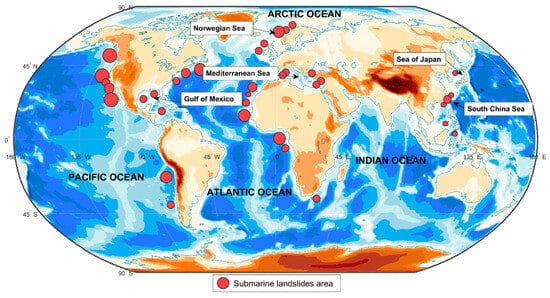
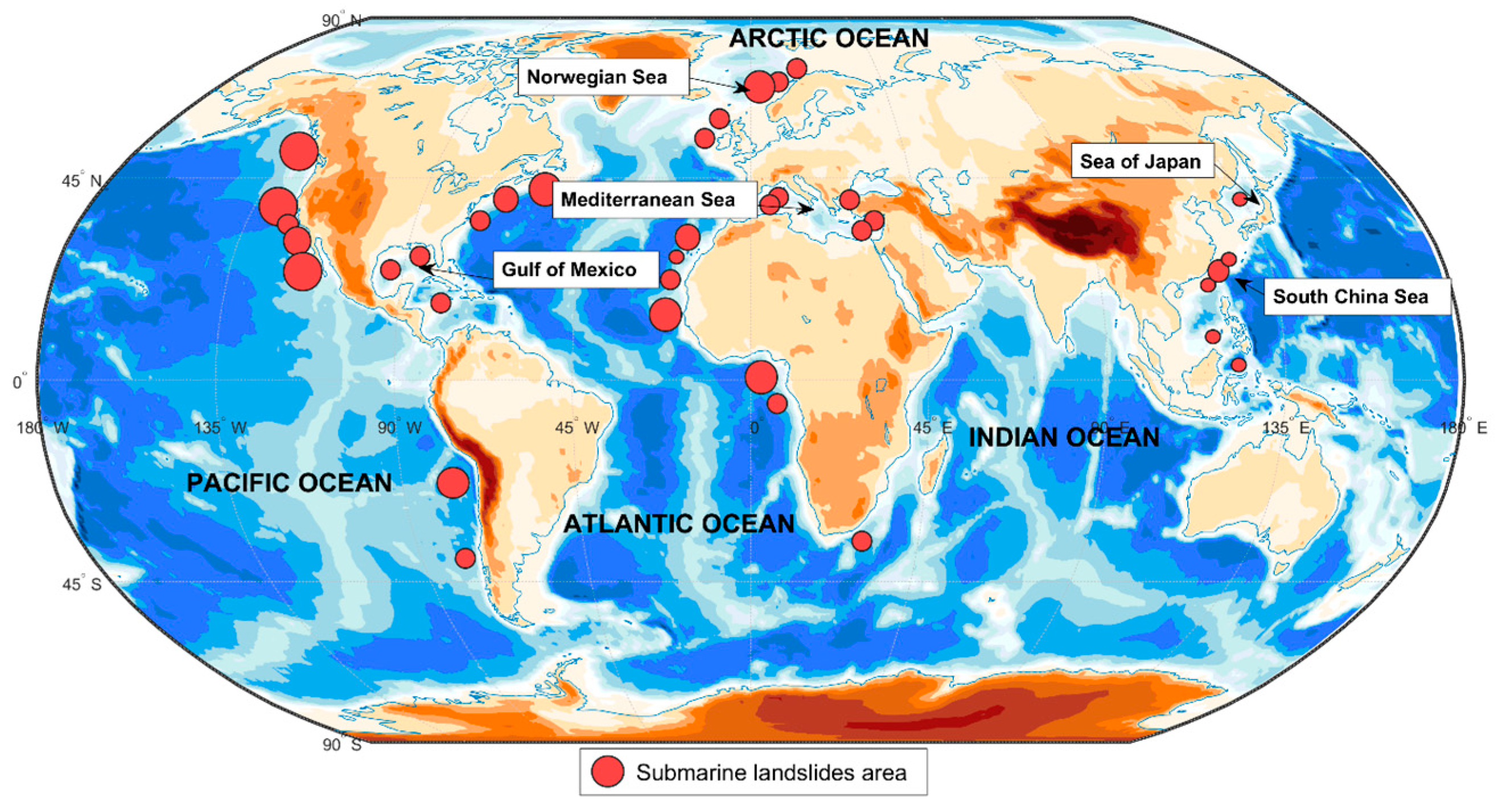
The 21st century marks a new era in the development and utilization of marine technology, with the ocean serving as a vast resource that makes sustainable development increasingly achievable for humanity [1,2]. As offshore oil and gas exploration expands, along with the construction of offshore wind turbines and platforms, gaining an accurate understanding of seabed geological conditions and sediment properties is essential for seabed stability assessment and early warning monitoring [3,4,5,6,7]. These evaluations are crucial for ensuring the safety of construction projects and the long-term serviceability of offshore infrastructure [8,9,10,11]. Submarine landslides have historically occurred in offshore regions where marine engineering projects are prevalent [12,13,14,15,16]. Figure 1 illustrates the regional distribution of areas prone to submarine landslide, where the size of the dots corresponds to the relative scale and volume of recorded landslide events.

Figure 1. Regional distribution of main areas prone to submarine landslides, where the size of the dots corresponds to the relative scale and volume of recorded landslide events (modified from [12]).

Offshore engineering projects, such as oil and gas exploitation and submarine pipeline installation, require precise predictions of sediment strength and stability. These predictions rely on the accurate characterization of sediment properties, including porosity and consolidation degree [17,18,19,20]. Resistivity and acoustic parameters serve as non-destructive indicators of these properties [21]. As offshore and marine structures continue to develop, research and methods for characterizing seafloor sediments have gained increasing attention. In particular, advancements in in situ and laboratory testing techniques for marine sediments have accelerated in recent years. The resistivity and acoustic properties of sediments are critical for accurate soil characterization, and understanding their relationships with other physical properties plays a fundamental role in marine sediment research. It is worth pointing out that unlike lacustrine or river sediments, marine sediment characterization must account for several unique environmental and compositional factors such as pore water salinity, hydrostatic pressure, and complex gas components.

Many studies have investigated the electrical resistivity and acoustic properties of seafloor sediments, resulting in a wealth of innovative findings. These studies primarily focus on factors influencing sediment resistivity and acoustic wave propagation [22,23], the development of in situ and laboratory measurement methods [24,25,26], correlations between resistivity and acoustic parameters with other sediment properties [27], and the creation of theoretical models and empirical prediction equations based on observed data [28].

Despite the extensive research on resistivity and acoustic testing, two critical gaps remain: (1) the absence of a systematic comparison of in situ techniques regarding their resolution, cost, and field applicability; (2) and the insufficient discussion on acoustic model performance for gas hydrate-bearing sediments [29], where sediment structure changes dynamically. This review aims to address these gaps by synthesizing recent advancements and providing actionable insights for future research directions.

2. Resistivity Measurements

Archie [30] was the first to apply resistivity measurements to study the microstructural characteristics of saturated sandstone. He introduced the concept of the soil’s structural factor, denoted as f_s, defined as the ratio of the soil resistivity (r_s) to pore water resistivity (r_w). However, to better account for the influence of complex pore geometry and tortuosity, Winsauer et al. [31] refined this relationship into the following model:

$$f_s={\displaystyle \frac{r_s}{r_w}}=\beta {\varphi }^{-m}$$

(1)

where ϕ is the porosity, m is the cementation factor, and β is the tortuosity factor (also known as the lithology constant). Both β and m are empirical constants dependent on the composition and structure of the sediments.

While Equation (1) is the most common expression, it has undergone significant reappraisal to account for complex pore geometries and different conducting phases, as detailed in the comprehensive review by Glover [23]. The structural factor is not merely a geometric ratio but a reflection of the connectivity and tortuosity of the pore network within the sediment matrix [23].

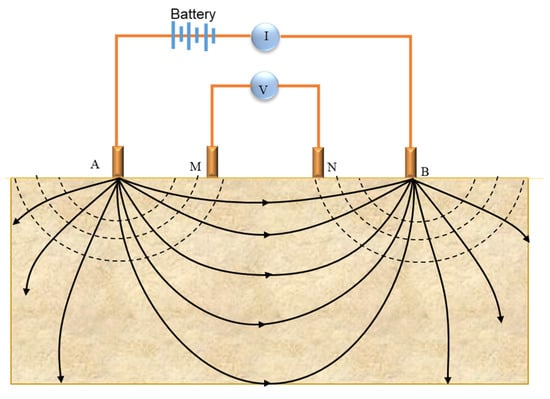
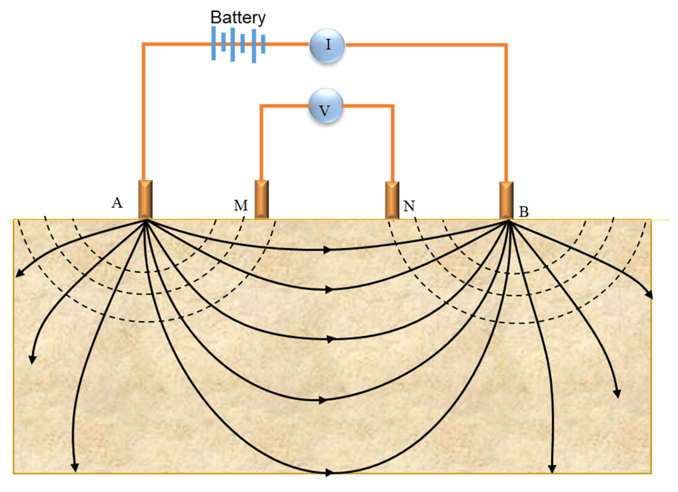
To measure resistivity in seafloor sediments, the Wenner array is employed (as shown in Figure 2) [32], which is defined as a linear configuration of four electrodes with equal spacing (a). In this setup, a constant current (I) is applied through the current electrodes (A and B), while the resulting voltage drop (ΔV) is measured across the measuring electrodes (M and N). Based on the potential distribution in a semi-infinite homogeneous medium, the resistivity is expressed as

$$r_s={\displaystyle \frac{2\pi a\mathrm{\Delta }V}{I}}$$

(2)

Figure 2. Schematic of soil resistivity measurement using the Wenner array (modified from [32]).

2.1. In Situ Measurement of Sediment Resistivity

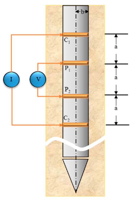
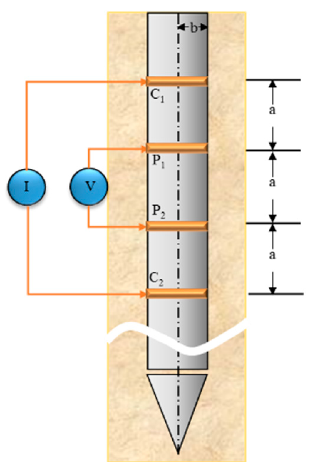
The development of in situ resistivity probes for marine environments dates back to the late 1960s. Kermabon et al. [27] first developed a deep-sea electrical resistivity probe equipped with a four-point electrode array at its tip. This 13 m long instrument was designed to obtain continuous resistivity–depth profiles by pressing the electrodes against the sediment during the controlled extraction of the probe from the seafloor. Building upon this foundational configuration, Won [33] later refined the theoretical calculation of the geometrical factor for ring electrodes and used a Wenner configuration with four ring electrodes for field testing to measure the electrical properties of seafloor sediment. The ring electrodes were evenly spaced along the surface of a probe rod, typically made of Perspex or other insulating materials, allowing for the detection of electrical properties in seafloor sediments. The Wenner configuration, employing four ring electrodes, is depicted in Figure 3. The resistivity measured by these four ring electrodes in the field is calculated using the following equation:

$$r_s=4\pi G{\displaystyle \frac{\mathrm{\Delta }V}{I}}$$

(3)

where G is the geometrical factor, which is determined by the electrode shape and layout configuration, and can be calculated as

$$G={\displaystyle \frac{\pi b}{4}}{\left[\ln {\displaystyle \frac{4a+2\pi b}{4a+\pi b}}\right]}^{-1}$$

(4)

where a is the spacing between adjacent electrodes, and b is the radius of the ring electrode. Ridd [34] further improved the accuracy of this measurement by refining the theoretical calculations and analysis of the electrical potential across the four ring electrodes.

Figure 3. Wenner configuration of four ring electrodes (modified from [33]).

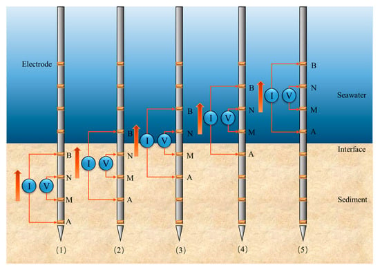
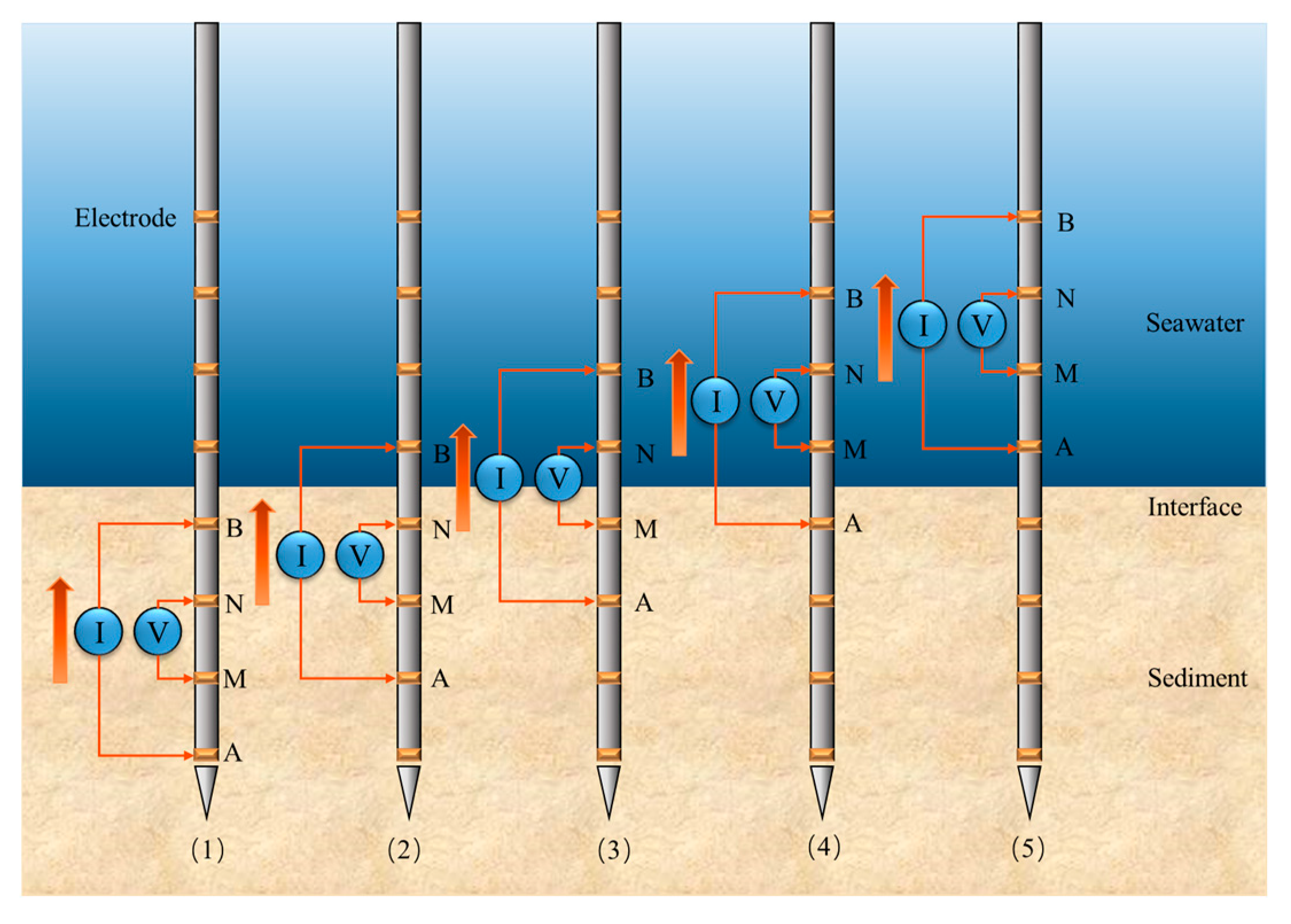
Jia et al. [25] conducted field resistivity monitoring during the sediment consolidation process in the Yellow River estuary in China using a Multi-electrode Resistivity Measurement System (MRMS) with a probe rod equipped with ring electrodes. The measuring process using the probe, controlled by multi-Wenner arrays, is illustrated in Figure 4. This system enabled the acquisition of a comprehensive resistivity profile by sequentially switching the Wenner arrays upward until all electrodes were engaged. It was found that sediment resistivity is a crucial parameter in the consolidation process, with porosity being the primary factor influencing resistivity. As pore pressure dissipated and porosity decreased, resistivity gradually increased [35]. An empirical formula was derived from experimental data to predict the degree of consolidation in marine sediments at the Yellow River estuary. Other probe-based systems have also been developed to withstand the challenges of deep-sea environments. Rosenberger et al. [36] designed a free-fall in situ resistivity probe for deep-water sediments, utilizing a modular design that allows for autonomous operation and high-resolution profiling in water depths exceeding 4000 m.

Figure 4. Measurement process employing the Wenner array configuration controlled by MRMS (modified from [25]).

Beyond local probe measurements, large-scale characterization of marine sedimentary structures has been revolutionized by electromagnetic methods. The field was pioneered by Chip Cox [37], whose foundational work on marine controlled-source electromagnetic (CSEM) and marine magnetotellurics (MT) provided the theoretical and practical basis for deep-sea resistivity exploration. Building on this legacy, Constable et al. [38] successfully utilized CSEM data in the San Diego Trough to map complex offshore sedimentary structures, demonstrating how electromagnetic induction can resolve vertical resistivity variations at scales far exceeding traditional probe capabilities. In recent years, Bialas et al. [39] measured the resistivity of the Danube deep-sea fan region in the Black Sea by CSEM data using two instrument systems. The first method involved a 2D seafloor towed system, consisting of a 100 m long horizontal transmitter dipole and up to five receiving dipoles. The second method employed a 3D stationary system, using twelve ocean-bottom electromagnetic receivers (OBEM) deployed along two parallel lines, with an average spacing of 300 m. These electromagnetic data sets were processed through inversion to obtain resistivity–depth distribution models. The study showed that the electrical resistivity of sediment formations depends on porosity and pore fluid resistivity. Gas hydrate and free gas have much higher electrical resistivities than saline pore fluid.

Zhang et al. [40] used the Electrical Resistivity Tomography (ERT) method to monitor the groundwater discharge process at Shilaoren Beach, Qingdao, China, during both rainy and dry seasons. A dipole–dipole array of 100 equally spaced stainless-steel electrodes was deployed along a 247.5 m profile perpendicular to the shoreline. Each measurement took approximately 13 min, and the apparent resistivity data was inverted using software to generate true resistivity profiles. The study found that in coastal saturated sediments, changes in pore water salinity are the primary factor affecting resistivity over short periods. A summary of the above-mentioned in situ resistivity measurement methods is provided in Table 1.

Table 1. Summary of in situ resistivity measurement methods.

Researcher	Method	Electrode Design	Applicable Sediment Type	Advantages	Limitations
Won [33]	Wenner array (4 rings)	4 ring electrodes on probe	Loose shallow sediments	Simple structure, low cost	Low resolution; sensitive to probe tilt
Jia et al. [25]	MRMS (multi-Wenner)	Multiple ring electrodes	Estuarine consolidated sediments	High-resolution profiles; continuous measurement	Limited to shallow waters
Bialas et al. [39]	CSEM (2D/3D)	Towed dipole + OBEM	Deep-sea fan sediments (Black Sea)	Large-scale exploration; deep penetration	High cost; long data acquisition time
Zhang et al. [40]	ERT (dipole–dipole)	100 stainless-steel electrodes	Coastal saturated sediments	High temporal resolution; anti-noise	Requires shore-based deployment; not for deep sea

From the comparison, it is evident that no single in situ resistivity method is universally applicable. For shallow estuarine sediments (e.g., Yellow River estuary), MRMS is preferred for high-resolution consolidation monitoring, while CSEM is better suited for deep-sea large-scale exploration (e.g., Danube deep-sea fan), though it sacrifices resolution. Future research should focus on hybrid methods to balance resolution and exploration scale.

2.2. Laboratory Resistivity Measurements

2.2.1. Consolidation Apparatus with Electrodes

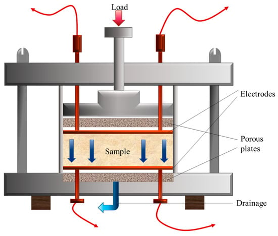
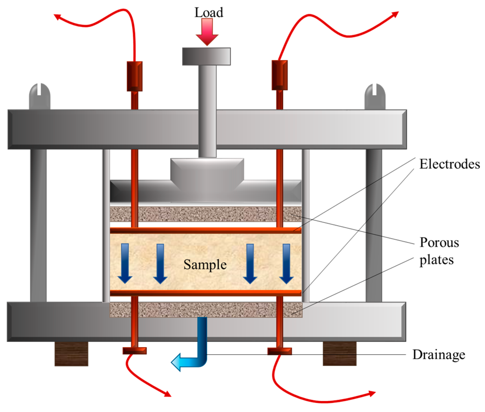
Fukue et al. [41] used a device, shown in Figure 5, to investigate the microstructures and resistivity characteristics of clay. This apparatus, which resembled a standard consolidometer, included stainless-steel electrodes affixed to both the top and bottom of the sample. Unlike the Wenner array configuration, this system utilized a 0.1 mA, 1 kHz alternating current (AC) to measure electrical resistivity during the consolidation process and develop a structural model to characterize soil microstructure.

Figure 5. Consolidation apparatus with electrodes (modified from [41]).

2.2.2. Multi-Electrode Board

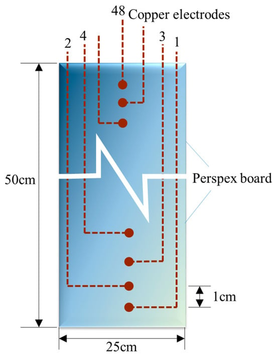
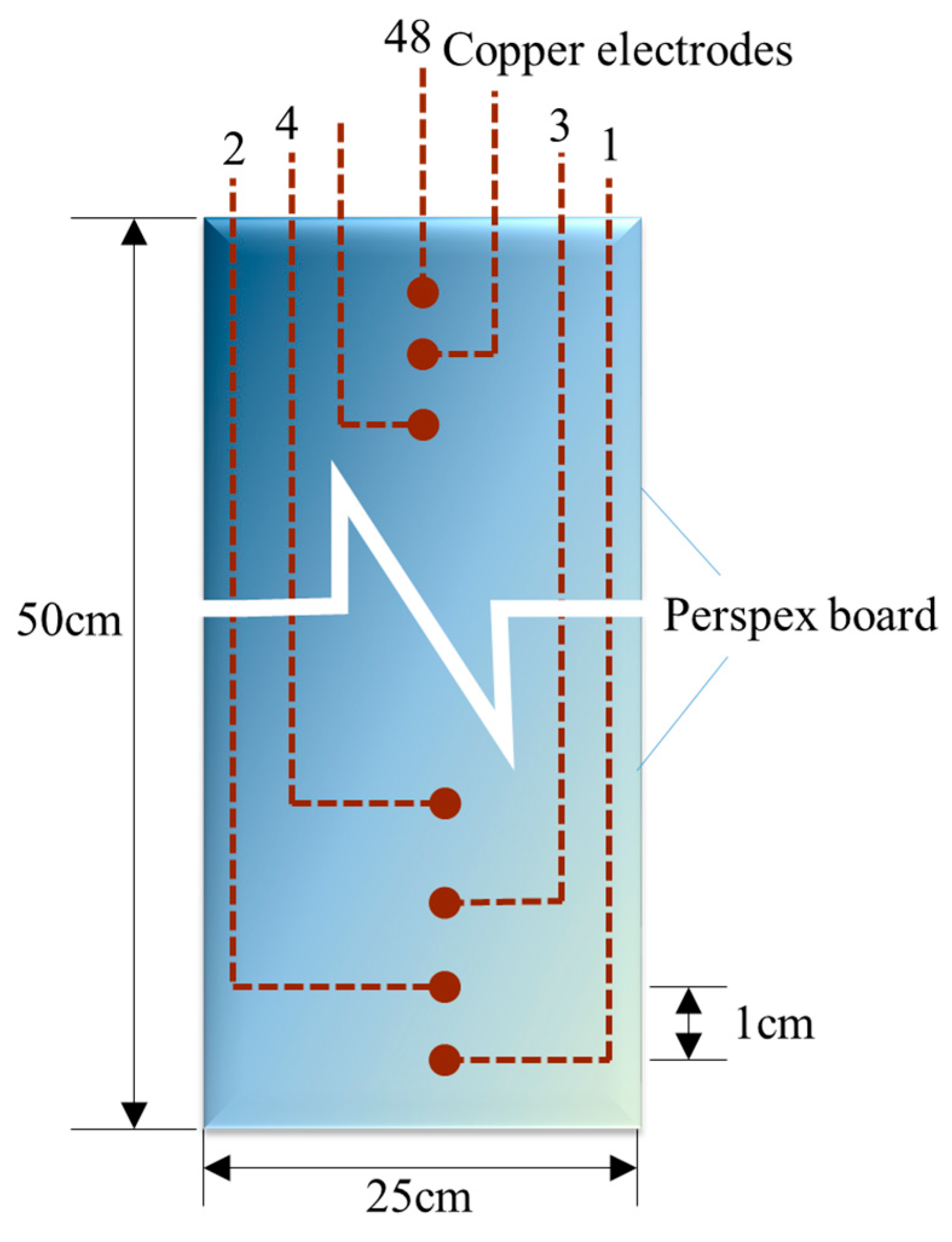
In laboratory settings, Liu and Jia [35] employed a multi-electrode board (25 cm × 50 cm) to measure the electrical resistivity of marine sediments collected from the Yellow River estuary. The board featured 48 cylindrical copper cables spaced at 1 cm × 1 cm intervals as shown in Figure 6. The electrodes were numbered sequentially from 1 to 48, allowing for continuous measurement of resistivity in the vertical direction by systematically changing sets of four electrodes.

Figure 6. Diagram of the electrode board used in laboratory experiments (modified from [35]).

2.2.3. Precision LCR Meter

Xing et al. [42] connected a precision LCR meter to the copper electrodes at both ends of the reactor to measure raw impedance data within a frequency range of 20 Hz to 1 MHz. The signals from the sensors were processed by a transmitter and current–voltage converter, and the data were transmitted to a control computer integrated with custom software for analysis. A summary of the above-mentioned laboratory resistivity measurement methods is provided in Table 2.

Table 2. Summary of laboratory resistivity measurement methods.

Method	Equipment	Principle	Advantages	Limitations	Representative Study
Consolidation apparatus	Consolidometer + electrodes	AC impedance under loading	Monitors consolidation vs. microstructure	Electrode polarization	Fukue et al. [41]
Multi-electrode board	Perspex board + 48 copper electrodes	DC scanning (Wenner array)	Non-destructive; fast; continuous	Resolution limited by spacing	Liu and Jia [35]
Precision LCR meter	LCR meter + copper electrodes	Frequency-domain analysis	High precision; wide frequency range	High cost; noise sensitive	Xing et al. [42]

3. Acoustic Measurements

3.1. Theoretical Models of Acoustic Wave Propagation

The methods for determining acoustic parameters of seafloor sediments include theoretical model prediction, empirical equations, and direct acoustic parameter measurements. Sediment acoustic wave propagation theories primarily encompass fluid theory, elastic theory, and poroelastic theory, each treating seafloor sediments as a fluid, elastic solid, or porous elastic medium, respectively.

In fluid theory, seafloor sediments are treated as continuous media. The acoustic velocity is derived from the Wood equation [43], which defines the material properties based on the average physical parameters within a unit volume:

$$\begin{array}{c}{\rho }_0=N{\rho }_w+(1-N){\rho }_g\\ 1/K_b=N/K_w+(1-N)/K_g\\ c_0=\sqrt{{\displaystyle \frac{K_b}{{\rho }_0}}}\end{array}$$

(5)

where ρ₀ is the equivalent density and K_b is the bulk modulus of the sediment unit, with N, ρ_w, ρ_g, K_w, and K_g representing porosity, water density, sediment particle density, water bulk modulus, and sediment particle bulk modulus, respectively. According to the above equation, the acoustic velocity of sediments can be obtained as

$$c_0=\sqrt{{\displaystyle \frac{K_g{K}_w}{\left[N{\rho }_w+(1-N){\rho }_g\right]\left[N{K}_g+(1-N)K_w\right]}}}$$

(6)

While this equation provides a foundational low-frequency limit for fluid-saturated sediments, it primarily serves as a simplified baseline as it neglects the skeletal frame’s stiffness and the relative motion between the pore fluid and the particles.

The elastic theory, on the other hand, considers the elastic properties of solid particles and shear forces, which are not addressed in fluid theory. The Buckingham model assumes sediment particles are in contact but not cemented [44]. The acoustic velocity of these sediments at a single frequency can be approximated by [45]

$$c_p=\sqrt{c_0^2+({\displaystyle \frac{u_g}{u_0}}{)}^{1/3}{\displaystyle \frac{{\mu }_0}{{\rho }_0}}}$$

(7)

where µ₀ is the friction stiffness constant of the longitudinal wave (2 × 10⁹ Pa), u_g is the particle size of the sediment (with a reference value of u₀ = 1000 µm). ρ₀ and c₀ are the same as those in the Wood equation.

The Buckingham model offers a more sophisticated approach by incorporating the elastic properties of solid particles and shear forces. Although earlier versions faced challenges in describing gas-bearing sediments, the updated Buckingham model [22] has significantly improved the analysis of shear wave attenuation in unconsolidated sands. Recent comparative studies have reaffirmed its utility. For instance, Lee et al. [46] showed that in certain in situ environments, the Buckingham model can provide more accurate predictions for sound speed and attenuation than the more complex Biot–Stoll poroelastic theory. Consequently, the choice between these models depends on the specific sediment composition and the frequency range of interest.

The Biot–Stoll theory remains a comprehensive poroelastic theory, incorporating both the porosity and elasticity of the medium [47,48,49,50,51,52]. This theory posits that the dissipation of energy in the sediment skeleton contributes to the attenuation of acoustic energy. The real and complex moduli of the fluid, sediment particles, and the skeletal framework are

$$\begin{array}{c}\overline{H}={\displaystyle \frac{(K_g-{\overline{K}}_b{)}^2}{D-{\overline{K}}_b}}+{\overline{K}}_b+{\displaystyle \frac{4}{3}}{\overline{\mu }}_b\\ \overline{C}={\displaystyle \frac{K_g(K_g-{\overline{K}}_b)}{D-{\overline{K}}_b}}\\ \overline{M}={\displaystyle \frac{K_g^2}{D-{\overline{K}}_b}}\end{array}$$

(8)

where

$$D=K_g+{\displaystyle \frac{K_g^2}{K_w}}N-K_{g}N$$

(9)

${\overline{K}}_b$ and ${\overline{\mu }}_b$ are the bulk modulus and shear modulus of the assemblage of particles comprising the frame. In the formula, K_g and K_w are assumed to be real constants whereas ${\overline{K}}_b$ and ${\overline{\mu }}_b$ are assumed to be a complex number in order to account for the various forms of energy dissipation that occur at the grain contacts.

The characteristic equation derived from Biot–Stoll theory can be used to determine the velocity and attenuation of shear waves:

$$\left|\left.\begin{array}{cc}H{t}^2-\rho {\omega }^2& {\rho }_w{\omega }^2-C{t}^2\\ C{t}^2-{\rho }_w{\omega }^2& m_a{\omega }^2-M{t}^2-i{\displaystyle \frac{\omega F\eta }{k}}\end{array}\right|\right.=0$$

(10)

where ρ is total mass density, t is the complex wave number, η is fluid viscosity, k is the permeability coefficient of the porous framework, ω is the angular frequency, m_a is an apparent mass, and F is a complex correction factor. Then, the velocity c_b is

$$c_b=\mathit{Re}({\displaystyle \frac{\omega }{t}})$$

(11)

where Re (x) is the real part of the complex number x.

3.2. In Situ Measurements of Acoustic Parameters

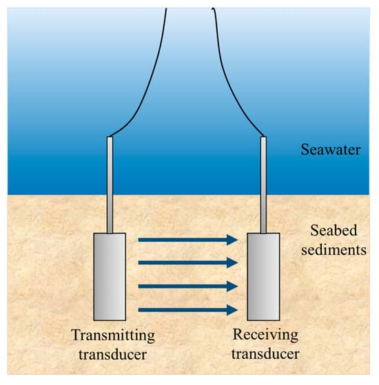
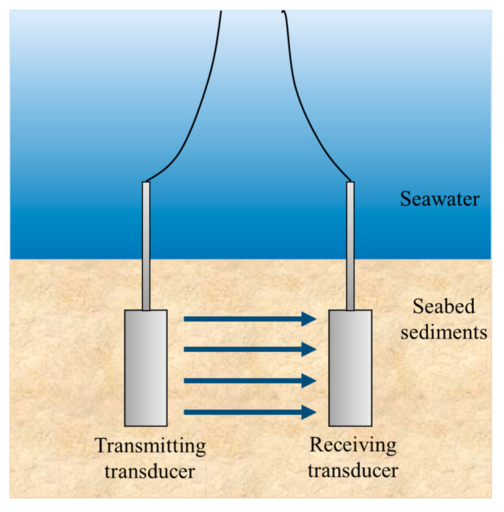
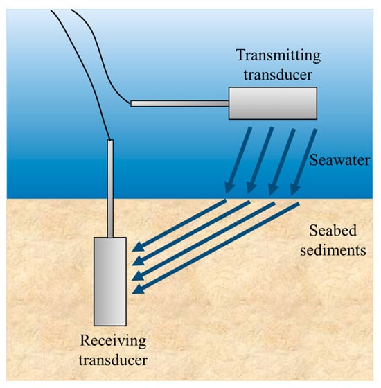
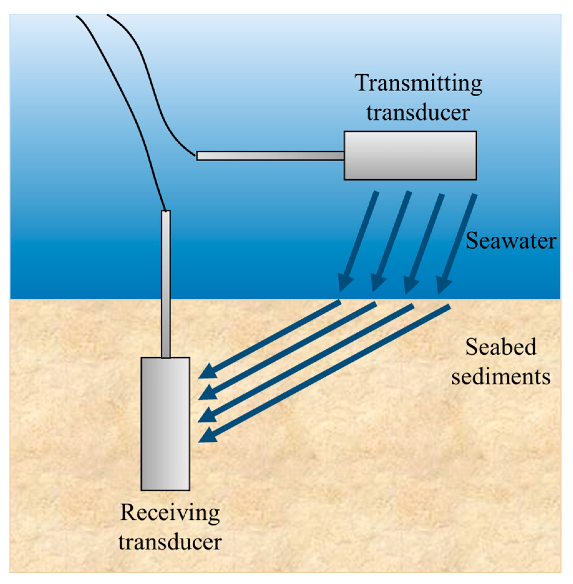
Since the 1950s, the acoustic velocity and sound attenuation in loose sediments have been measured using a variety of methods. These include laboratory measurements, in situ subsurface acoustic measurements, and acoustic remote sensing. Environmental conditions change the acoustic properties of the sediments by influencing the physical parameters of marine sediments. Two main types of in situ acoustic measurement methods are distinguished by how the ultrasonic wave travels through the sediments: transmission-based and refraction-based methods. The principles of these methods are illustrated in Figure 7 and Figure 8 [53].

Figure 7. Principle of transmission-based in situ acoustic measurement.

Figure 8. Principle of refraction-based in situ acoustic measurement.

Acoustic velocity (c_p) and sound attenuation coefficient (α) are calculated by the following expression:

$$c_p=c_w/(1-{\displaystyle \frac{c_w\mathrm{\Delta }t}{d}})$$

(12)

$$\alpha =20\log ({\displaystyle \frac{A_w}{A_s}})/d$$

(13)

where c_w is the acoustic velocity of overlying seawater, Δt is the time difference between the transmitting and receiving transducers, d is the propagation distance through the sediments, and A_w and A_s are the amplitude of the acoustic vibration received in the seawater and the sediment, respectively.

Several in situ acoustic measuring devices have been developed, including transmission-based systems such as the ARL/UT profilometer [54], ISSAMS (In Situ Sediment geoAcoustic Measurement System) [55,56,57,58], SAPPA (Sediment Acoustic & Physical Properties Apparatus) [59], ISSAP (In Situ Sound Speed and Attenuation Probe) [60], SPADE (Sediment Probing Acoustic Detection Equipment) [61], and Attenuation Array [62,63]. Refraction-based devices like the Acoustic Lance [64,65,66,67], Mini-boomer [68], and SAMS (Sediment Acoustic Measurement System) [69] are also widely used.

In addition to these traditional systems, newer advanced remote sensing and in situ measurement techniques are continuously emerging. For instance, Knobles et al. [70] conducted remote sensing seabed acoustics experiments using maximum entropy methods on pressure time series generated by explosive sources in the 25~275 Hz frequency band. Spica et al. [71] utilized Distributed Acoustic Sensing (DAS) technology, employing fiber-optic cables installed on the seafloor to record seismic data for high-resolution subsurface shear wave profiling. Lu et al. [72,73] analyzed the physical properties and acoustic characteristics of sediments in the South China Sea using VWA (Velocity–Wave–Amplitude) discrimination technique. Lee et al. [74] investigated acoustic characteristics of gas-bearing sediments in Jinhae Bay, in the southeast of Korea, using high-resolution seismic survey. Neto et al. [75] researched the relationship between geotechnical properties and the acoustic impedance of shallow marine sediments from the Santos Basin, Brazil. Zhan et al. [76] employed the Sonic Scope tool in the South China Sea, transmitting P- and S-waves through sediments. The tool’s array of 12 receivers, spaced 0.1 m apart, recorded the arrival times of sonic waveforms to determine sediment shear wave velocity. In their study, acoustic attenuation was not measured directly. It was calculated using a method proposed by Suzuki and Matsushima [77] through complex signal processing and frequency-domain analysis of the complete received waveforms. Acoustic characteristics of marine sediments in typical sea areas have been gradually revealed. Details of these measurement systems are summarized in Table 3.

Table 3. Summary of in situ measurement systems for acoustic properties of marine sediments.

Measurement Systems	Maximum Working Depth (m)	Maximum Measured Depth (m)	Measured Parameters	Frequency (kHz)	Transmission Distance (m)	Example
ARL/UT profilometer	7000	12	$V_p^h$$,{\alpha }_p^h$	200	-	Tucholke and Shirley [54]
Acoustic Lance	6000	5.00	$V_p^v$$,{\alpha }_p^v$	8	-	Gorgas et al. [64]
ISSAMS	-	0.3	$V_p^h$$,{\alpha }_p^h$, $V_s$$,{\alpha }_s$	P:60 S:0.25~1.5	P:0.58~1.00 S:0.30~0.70	Richardson et al. [55]
Mini-boomer	-	0.5	$V_p^v$$,{\alpha }_p^v$	0.2~1.5	-	Best et al. [68]
SAPPA	6000	1.0	$V_p^h$$,{\alpha }_p^h$$,V_s$,	P:1~100 S:0.07~0.17	-	Best et al. [59]
Attenuation Array	-	0.1	$V_p^h$$,{\alpha }_p^h$	40~300	0.22~0.44	Thorsos et al. [62]
ISSAP	-	0.15	$V_p^h$$,{\alpha }_p^h$	40,65	0.10~0.60	Mayer et al. [60]
SPADE	-	1.00	$V_p^h$$,{\alpha }_p^h$	10~100	0.99~8.10	Robb et al. [61]
SAMS	-	3.00	$V_p^v$$,{\alpha }_p^v$	2~35	1.18~2.97	Yang et al. [69]
DAS	Seafloor	Subsurface	$V_s$ profiling	Seismic band	-	Spica et al. [71]
VWA Discrimination	-	-	Physical and acoustic properties	-	-	Lu et al. [72]
Sonic Scope	-	-	$V_s$$,V_p$	10~20	1.83	Zhan et al. [76]

$V_p^h$: horizontal acoustic velocity; ${\alpha }_p^h$: horizontal acoustic attenuation coefficient; $V_p^v$: vertical acoustic velocity; ${\alpha }_p^v$: vertical acoustic attenuation coefficient; $V_s$: shear wave velocity; ${\alpha }_s$: shear wave attenuation coefficient; P: pressure wave; S: shear wave.

3.3. Laboratory Measurement of Acoustic Parameters

3.3.1. Acoustic Velocity Measurements

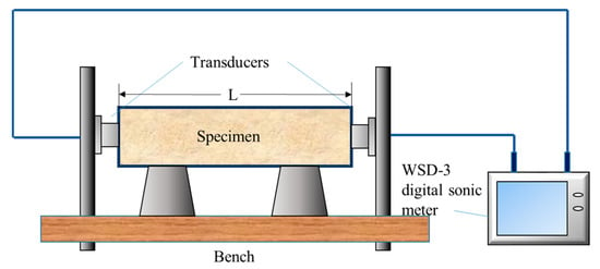
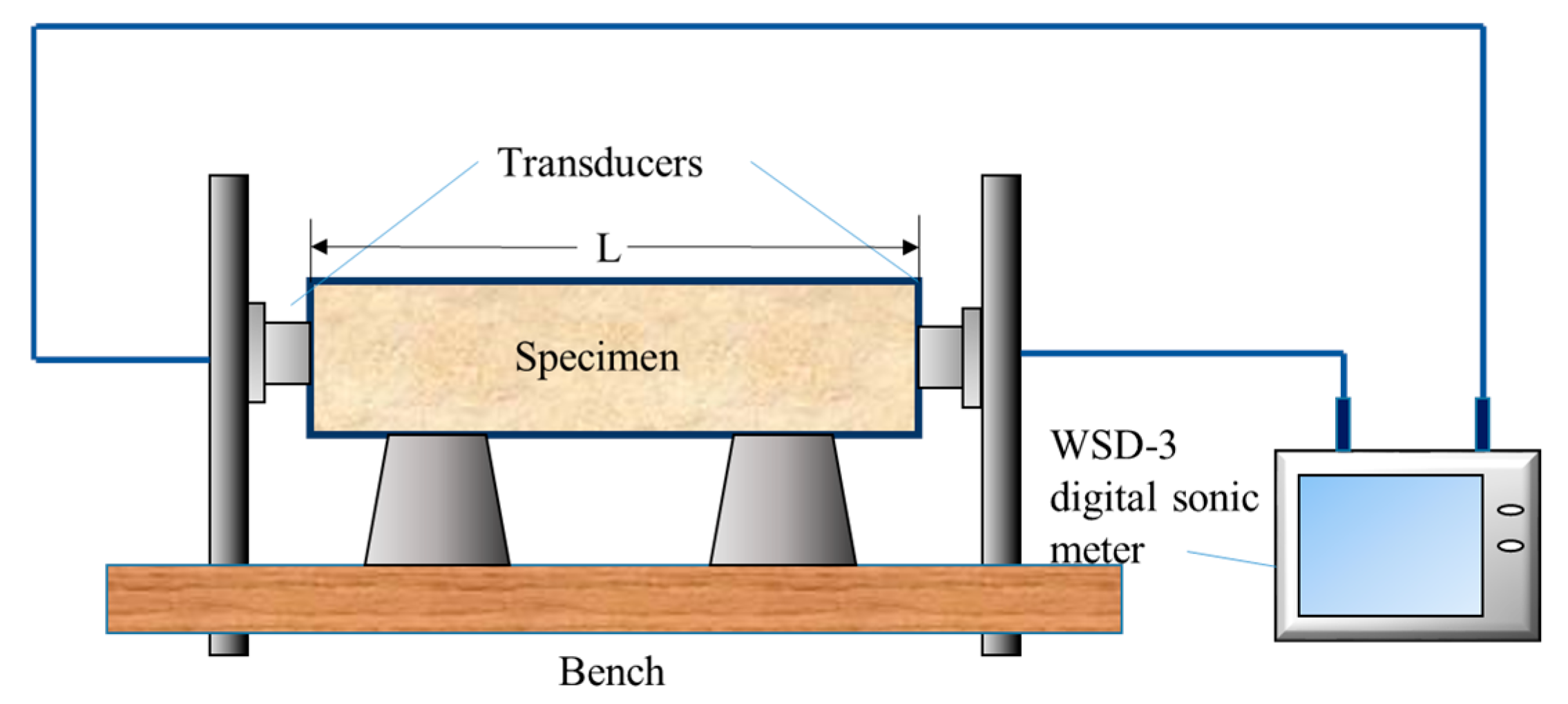
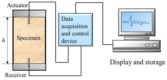
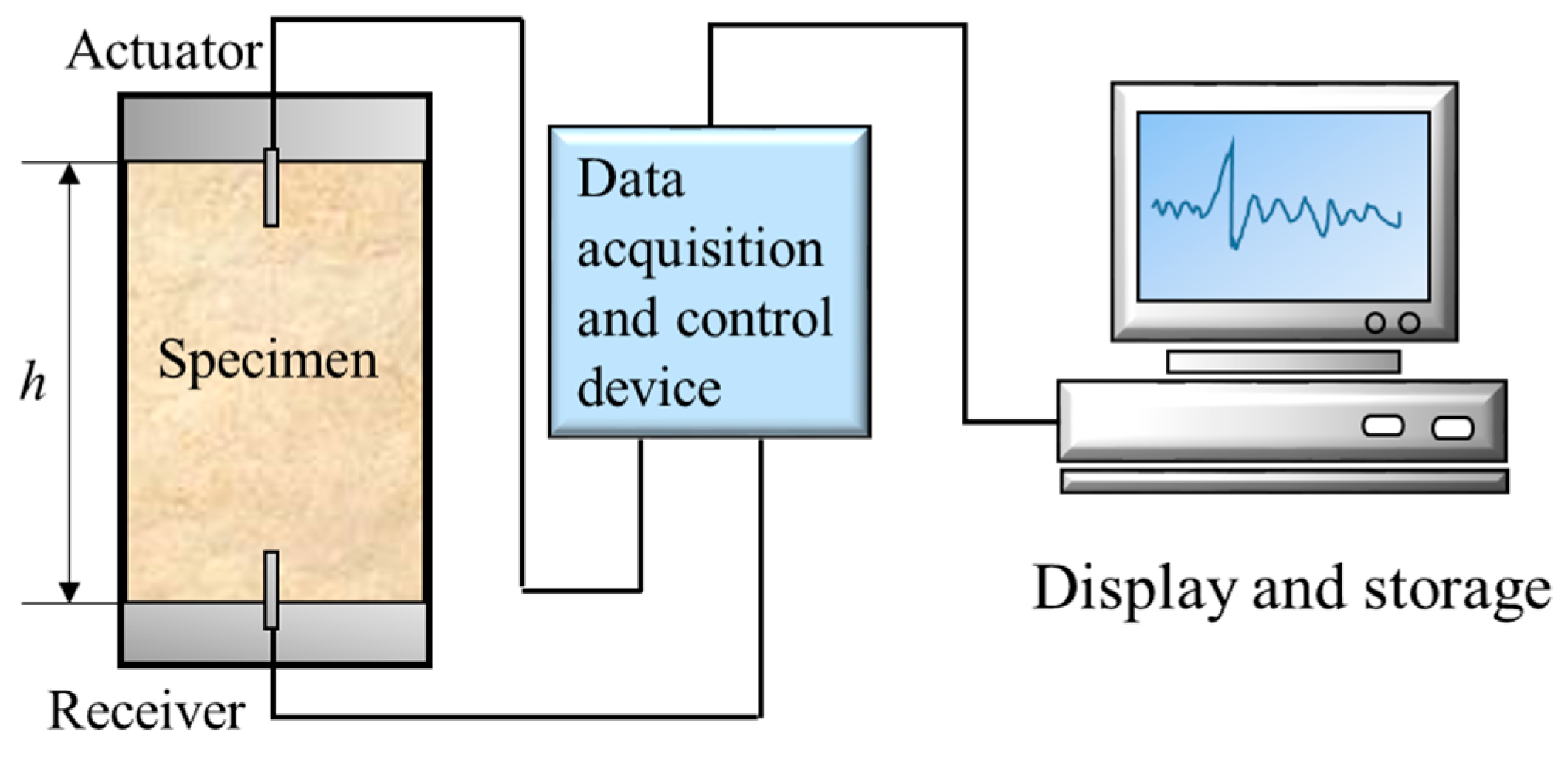
In laboratory experiments, acoustic velocity is typically measured using a WSD-3 digital sonic meter. The principle of measurement is shown in Figure 9. Acoustic waves generated by the transmitting transducer propagate through the sediment sample and are received by the receiving transducer. In the case of a known sample length, the sound wave penetration time is calculated based on the received signal recorded by the digital sonic meter. The velocity of sound can be calculated as

$$V_p={\displaystyle \frac{L}{t-t_1-t_0}}\times 10^3$$

(14)

where V_p is the acoustic velocity of the sample (m/s), L is the sample length (mm), t is the audio penetration time (μs), t₁ is the system delay (μs), and t₀ is the acoustic correction value (μs).

Figure 9. Acoustic system for measuring sediment sound velocity in the laboratory.

3.3.2. S-Wave Velocity Measurement

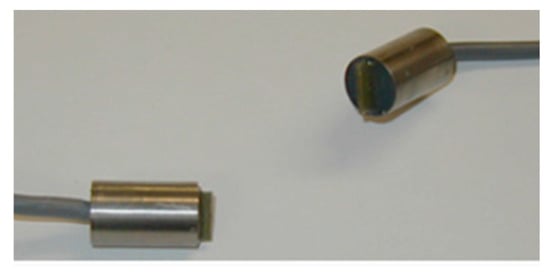
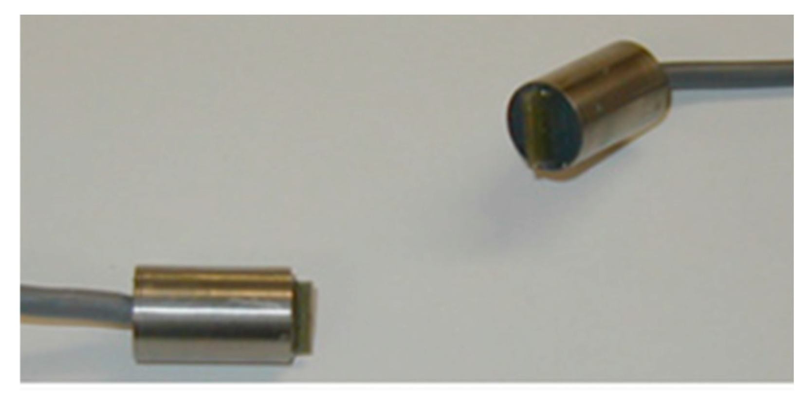
Shear wave velocity in sediments is commonly measured using bender elements in the laboratory [78,79]. A bender element is a typical mechanical–electrical sensor (Figure 10), which consists of two piezoelectric ceramic glued together. Both sides of the piezoelectric ceramic are coated with uniform electrodes.

Figure 10. Picture of bender elements.

Bender element can realize the conversion of mechanical energy and electric energy through the piezoelectric effect. In the shear wave velocity measurement for the soil, the bender element can be divided into an actuator and a receiver according to the function. The actuator produces vibration under the effect of the pulse voltage. Then, shear waves are generated and propagate through the soil to reach the receiver. The receiver vibrates and generates an electrical signal. The excitation signal is compared with the received signal and the time delay t between them, which is the propagation time of the shear wave, is measured [80,81]. Then, combined with the shear wave propagation distance h, the shear wave velocity Vs can be calculated.

$$V_s=h/t$$

(15)

Then, the small-strain shear modulus can be obtained according to elastic theory:

$$G_{max}=\rho V_S^2$$

(16)

where ρ is the density of soil.

The schematic of shear wave velocity measurement using the bender element method is shown in Figure 11 [82]. The dynamic shear modulus and damping characteristics of soft marine soil can be measured by combining the bender element with the cyclic triaxial test [83].

Figure 11. Schematic of shear wave speed measurement using bender elements.

3.3.3. A New Type of Bender Element Transducer

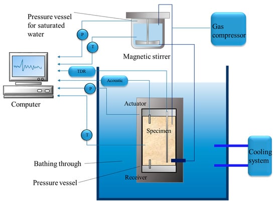
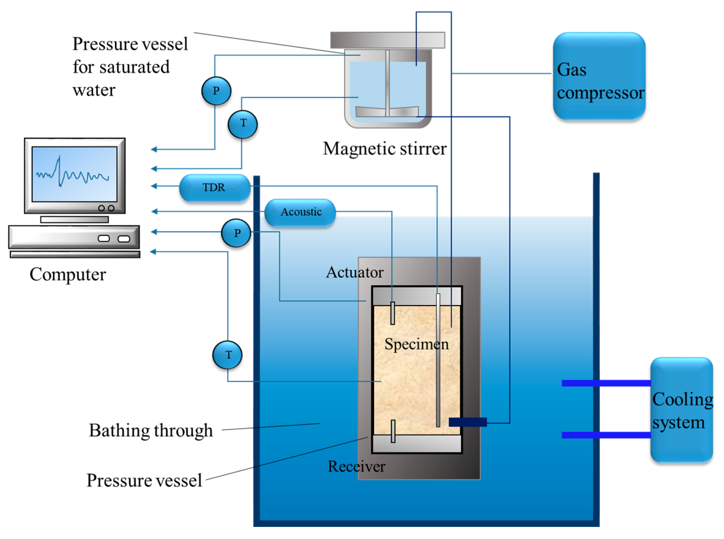
Hu et al. [84,85] proposed a novel bender element that can measure both the compressional wave velocity and shear wave velocity of hydrate-bearing unconsolidated sediments at the same time under certain pressure and temperature conditions. The experimental setup shown in Figure 12 includes the pressure vessel, the pressure vessel for saturated water, gas compressor, cooling system, and computer-control system. CH₄ was passed into the sediment sample, and the gas hydrate formation and decomposition processes were simulated by controlling the pressure and water bath temperature. The water content and the gas hydrate saturation parameters during hydrate formation were investigated using improved casting time-domain reflectometry (TDR). Temperature, pressure, acoustic, and TDR waveforms were recorded in real time by computer systems. The combination of Fast Fourier Transform (FFT) and Wavelet Transform (WT) were used to analyze both V_p and V_s data.

Figure 12. Experimental apparatus for researching acoustic properties of hydrate-bearing sediments (modified from [84]).

Just as described above, traditional transmitting and receiving transducers can only measure the compressional wave velocity, while bender elements can estimate the shear wave velocity of marine sediments. The new-type bender element proposed by Hu et al. [84] can measure the compressional and shear wave velocity at the same time, which is more efficient in the research of physical and mechanical characteristics of marine sediments.

3.3.4. Integrated Ultrasonic Monitoring During Creep Deformation

Hu et al. [26] proposed a novel device to test the time-dependent deformation and ultrasonic response of hydrate-bearing sediments (HBS) under high-pressure and low-temperature conditions. The experimental apparatus consists of a high-pressure chamber, an axial-load control system, and pressure systems that independently control confining pressure, pore pressure, and back pressure. Ultrasonic transducers are directly integrated into the top- and bottom-end caps of the sample chamber and are in close contact with the upper and lower faces of the columned HBS sample to improve the accuracy of acoustic testing. During the experimental process, creep loading was performed after maintaining a stable axial load on the device for more than 24 h. Upon reaching the preset load, axial strain, volumetric strain, and P- and S-wave signals were stored and monitored. The study indicated that acoustic velocity increased during the steady creep stage due to pore compaction, whereas it decreased rapidly during the accelerated creep stage due to crack penetration. A summary of the above-mentioned laboratory measurement systems for acoustic properties of marine sediments is provided in Table 4.

Table 4. Summary of laboratory measurement systems for acoustic properties of marine sediments.

Method	Wave Mode	Principle	Advantages	Example
Digital sonic meter	$V_p$	Based on wave penetration time and sample length	$\mathrm{Simple};\mathrm{reliable}{V}_p$	Tucholke and Shirley [54]
Bender elements	$V_s$, $G_{max}$	Piezoelectric conversion	$\mathrm{Direct}{G}_{max}$ measurement	Shirley and Hampton [78]
Novel bender element	$V_p,$ $V_s$	Combined analysis using FFT and WT	$\mathrm{Measures}\mathrm{both}{V}_p$$\mathrm{and}{V}_s$ simultaneously	Hu et al. [85]
Integrated Creep Monitor	$V_p,$ $V_s$	HBS under simulated high-pressure and low-temperature conditions	Measure acoustic parameters of HBS during creep deformation	Hu et al. [26]

4. Concluding Remarks

This review has summarized the state-of-the-art in situ and laboratory measurement techniques used to determine the electrical resistivity and acoustic properties of marine sediments. In summary, the selection of testing technology should be tailored to the specific sediment type and environment. For shallow estuarine sediments, probe-based systems like MRMS are effective for high-resolution consolidation monitoring. In contrast, deep-sea characterization requires large-scale techniques such as CSEM and OBEM receivers. Regarding acoustic characterization, while traditional transducers are primarily limited to longitudinal wave velocity, bender elements are essential for estimating shear wave velocity. The development of novel bender element transducers enables simultaneous V_p and V_s measurement, significantly enhancing the efficiency of physical–mechanical investigations. Furthermore, for gas hydrate-bearing sediments, new integrated devices now allow for real-time acoustic monitoring during triaxial creep deformation, revealing the dynamic coupling between mechanical failure and acoustic response.

Collectively, these studies have greatly advanced our understanding of the physical and mechanical behavior of marine sediments. The integration of resistivity and acoustic testing has provided a powerful framework for characterizing parameters such as porosity, saturation, and consolidation degree. Nevertheless, several critical challenges remain to be addressed in future research: (1) the low resolution in in situ resistivity detection, often caused by geometric constraints of probe design; (2) measurement errors arising from electrode polarization and the imperfect soil–electrode contact; (3) and inaccuracies in theoretical and empirical models linking geophysical parameters such as resistivity and acoustic velocity to geotechnical properties, particularly under complex conditions such as gas hydrate-bearing or highly heterogeneous sediments.

To overcome these challenges, future efforts should aim to (i) enhance spatial resolution through optimized electrode array configurations and advanced signal processing algorithms; (ii) develop robust calibration frameworks that integrate in situ measurements with laboratory data to reduce uncertainty; (iii) expand the operational range of testing equipment for deeper and harsher marine environments; and (iv) innovate non-contact and non-destructive sensing technologies, such as fiber-optic and electromagnetic-acoustic hybrid systems, to minimize sample disturbance and improve measurement reliability. Continued progress in these areas will not only improve the quantitative accuracy of marine sediment characterization but also support safer and more efficient offshore engineering applications, including foundation design, resource exploration, and seabed stability assessment.

References

- Winther, J.G.; Dai, M.; Ristthoff, J.P.; Hoel, A.H.; Li, Y.; Trice, A.; Morrissey, K.; Juinio-Meñez, M.A.; Fernandes, L.; Unger, S.; et al. Integrated ocean management for a sustainable ocean economy. Nat. Ecol. Evol. 2020, 588, 390–398. [Google Scholar] [CrossRef] [Scilit] [PubMed]
- Toro, N.; Robles, P.; Jeldres, R.I. Seabed mineral resources, an alternative for the future of renewable energy: A critical review. Ore Geol. Rev. 2020, 126, 103699. [Google Scholar] [CrossRef] [Scilit]
- Martins, M.C.I.; Carter, M.I.; Rouse, S.; Russell, D.J. Offshore energy structures in the North Sea: Past, present and future. Mar. Policy 2023, 152, 105629. [Google Scholar] [CrossRef] [Scilit]
- Capizzano, C.W.; Rhoads, A.C.; Croteau, J.A.; Taylor, B.G.; Guarinello, M.L.; Shumchenia, E.J. Mapping seafloor sediment distributions using public geospatial data and machine learning to support regional offshore renewable energy development. Geosciences 2024, 14, 186. [Google Scholar] [CrossRef] [Scilit]
- Yang, Q.; Zhu, B.; Hiraishi, T. Probabilistic evaluation of the seismic stability of infinite submarine slopes integrating the enhanced Newmark method and random field. Bull. Eng. Geol. Environ. 2021, 80, 2025–2043. [Google Scholar] [CrossRef] [Scilit]
- Zhu, B.; Sun, Y.; Wang, T.; Mo, P.; Han, Y.; Ren, Y.; Li, J. Oscillatory responses of a spatially random seabed in the vicinity of structures: Validation and application of the integrated CFD-SFEM. Ocean Eng. 2024, 314, 119733. [Google Scholar] [CrossRef] [Scilit]
- Zhu, B.; Yang, Q.; Wang, T.; Lu, M.; Mo, P.; Hiraishi, T.; Mase, H. Investigation on wave-induced responses of heterogeneous seabed around a buried pipeline based on nonstationary random field model. Comput. Geotech. 2024, 167, 106119. [Google Scholar] [CrossRef] [Scilit]
- Zhu, B.; Hiraishi, T.; Mase, H.; Baba, Y.; Pei, H.; Yang, Q. A 3-D numerical study of the random wave-induced response in a spatially heterogenous seabed. Comput. Geotech. 2021, 135, 104159. [Google Scholar] [CrossRef] [Scilit]
- Zhu, B.; Hiraishi, T.; Mase, H.; Pei, H.; Yang, Q. Probabilistic analysis of wave-induced dynamic response in a poroelastic sloping seabed using random finite element method. Ocean Eng. 2022, 252, 111231. [Google Scholar] [CrossRef] [Scilit]
- Zhu, B.; Yang, Q.; Hiraishi, T.; Mase, H.; Pei, H.; Wang, T.; Lu, M. A stochastic numerical model for wave-induced dynamic response in a spatially heterogeneous seabed around structures. Ocean Eng. 2023, 288, 115789. [Google Scholar] [CrossRef] [Scilit]
- Liu, K.F.; Hsu, Y.C.; Chen, Y.C.; Lin, Y.Y. Deep sea water pumping pipe destruction due to undersea debris flow. Geoenviron. Disasters 2025, 12, 14. [Google Scholar] [CrossRef] [Scilit]
- Zhu, B.; Pei, H.; Yang, Q. Probability analysis of submarine landslides based on the Response Surface Method: A case study from the South China Sea. Appl. Ocean Res. 2018, 78, 167–179. [Google Scholar] [CrossRef] [Scilit]
- Zhu, B.; Pei, H.; Yang, Q. Reliability analysis of submarine slope considering the spatial variability of the sediment strength using random fields. Appl. Ocean Res. 2019, 86, 340–350. [Google Scholar] [CrossRef] [Scilit]
- Sun, Y.; Huang, B. A potential tsunami impact assessment of submarine landslide at Baiyun depression in Northern South China Sea. Geoenviron. Disasters 2014, 1, 7. [Google Scholar]
- Liu, X.; Wang, Y.; Zhang, H.; Guo, X. Susceptibility of typical marine geological disasters: An overview. Geoenviron. Disasters 2023, 10, 10. [Google Scholar] [CrossRef] [Scilit]
- Wang, Z.; Zheng, D.; Guo, X.; Gu, Z.; Shen, Y.; Nian, T. Investigation of offshore landslides impact on bucket foundations using a coupled SPH–FEM method. Geoenviron. Disasters 2024, 11, 2. [Google Scholar] [CrossRef] [Scilit]
- Kuznetsova, O.V.; Timerbaev, A.R. Marine sediment analysis—A review of advanced approaches and practices focused on contaminants. Anal. Chim. Acta 2022, 1209, 339640. [Google Scholar] [CrossRef] [Scilit] [PubMed]
- Wang, J.; Kan, G.; Li, G.; Meng, X.; Zhang, L.; Chen, M.; Liu, C.; Liu, B. Physical properties and in situ geoacoustic properties of seafloor surface sediments in the East China Sea. Front. Mar. Sci. 2023, 10, 1195651. [Google Scholar] [CrossRef] [Scilit]
- Yang, G.; Shan, H.; Nian, T.; Liu, J.; Sun, Y.; Xie, Z.; Zhu, C.; Liu, X.; Song, Y.; Sun, J.; et al. First in-situ full deep sea sediment strength testing device: MEGE. J. Mar. Environ. Eng. 2023, 11, 21–39. [Google Scholar]
- Zhong, K.; Chen, M.; Xie, C.; Zheng, J.; Chen, W.; Ou, W.; Yu, C. Design and application of a deep-sea engineering geology in situ test system. Minerals 2023, 13, 184. [Google Scholar] [CrossRef] [Scilit]
- Li, G.; Wang, J.; Meng, X.; Hua, Q.; Kan, G.; Liu, C. Seafloor sediment acoustic properties on the continental slope in the Northwestern South China Sea. J. Mar. Sci. Eng. 2024, 12, 545. [Google Scholar] [CrossRef] [Scilit]
- Buckingham, M.J. Analysis of shear-wave attenuation in unconsolidated sands and glass beads. J. Acous. Soc. Am. 2014, 136, 2478–2488. [Google Scholar] [CrossRef] [Scilit]
- Glover, P.W.J. Archie’s law—A reappraisal. Solid Earth 2016, 7, 1157–1169. [Google Scholar] [CrossRef] [Scilit]
- Guo, J.; Chen, J.; Zhou, P.; Han, B.; Chen, J.; Ren, Z. Subsea Multifrequency in situ sediment acoustic characteristics measurement system. IEEE Trans. Instrum. Meas. 2025, 74, 1–11. [Google Scholar] [CrossRef] [Scilit]
- Jia, Y.; Li, H.; Meng, X.; Liu, X.; Shan, H. Deposition-monitoring technology in an estuarial environment using an electrical-resistivity method. J. Coast. Res. 2012, 28, 860–867. [Google Scholar]
- Hu, Q.; Li, Y.; Sun, X.; Chen, M.; Bu, Q.; Gong, B. Integrating test device and method for creep failure and ultrasonic response of methane hydrate-bearing sediments. Rev. Sci. Instrum. 2023, 94, 025105. [Google Scholar] [CrossRef] [Scilit]
- Kermabon, A.; Gehin, C.; Blavier, P. A deep-sea electrical resistivity probe for measuring porosity and density of unconsolidated sediments. Geophysics 1969, 34, 554–571. [Google Scholar] [CrossRef] [Scilit]
- Jackson, D.R.; Richardson, M. High-Frequency Seafloor Acoustics; Springer Science and Business Media: New York, NY, USA, 2007. [Google Scholar]
- Yang, X.-D.; Chun, M.-H.; Luo, X.-Q.; Yao, Z.-G. Forward modelling and identification of shallow gas in the Bohai Bay seabed. Geoenviron. Disasters 2022, 9, 9. [Google Scholar] [CrossRef] [Scilit]
- Archie, G.E. The electrical resistivity log as an aid in determining some reservoir characteristics. Trans. AIME 1942, 146, 54–62. [Google Scholar] [CrossRef] [Scilit]
- Winsauer, W.O.; Shearin, H.M., Jr.; Masson, P.H.; Williams, M. Resistivity of brine-saturated sands in relations to pore geometry. Am. Assoc. Petrol. Geol. Bull. 1952, 36, 253. [Google Scholar]
- Wenner, F. A method of measuring earth resistivity. Bull. Bur. Stand. 1916, 12, 469–478. [Google Scholar] [CrossRef] [Scilit]
- Won, I. The geometrical factor of a marine resistivity probe with four ring electrodes. IEEE J. Ocean. Eng. 1987, 12, 301–303. [Google Scholar] [CrossRef] [Scilit]
- Ridd, P.V. Electric potential due to a ring electrode. IEEE J. Ocean. Eng. 1994, 19, 464–467. [Google Scholar] [CrossRef] [Scilit]
- Liu, X.; Jia, Y.; Zheng, J.; Shan, H.; Li, H. Field and laboratory resistivity monitoring of sediment consolidation in China’s Yellow River estuary. Eng. Geol. 2013, 164, 77–85. [Google Scholar] [CrossRef] [Scilit]
- Rosenberger, A.; Weidelt, P.; Spindeldreher, C.; Heesemann, B.; Villinger, H. Design and application of a new free fall in situ resistivity probe for marine deep water sediments. Mar. Geol. 1999, 160, 327–337. [Google Scholar] [CrossRef] [Scilit]
- Cox, C. Electromagnetic induction in the oceans and inferences on the constitution of the earth. Geophys. Surv. 1980, 4, 137–156. [Google Scholar] [CrossRef] [Scilit]
- Constable, S.; Key, K.; Lewis, L. Mapping offshore sedimentary structure using electromagnetic methods and terrain effects in marine magnetotelluric data. Geophys. J. Int. 2009, 176, 431–442. [Google Scholar] [CrossRef] [Scilit]
- Bialas, J.; Bohlen, T.; Dannowski, A.; Eisenberg-Klein, G.; Gassner, L.; Gehrmann, R.; Heeschen, K.; Hölz, S.; Jegen, M.; Klaucke, I.; et al. Joint interpretation of geophysical field experiments in the danube deep-sea fan, Black Sea. Mar. Pet. Geol. 2020, 121, 104551. [Google Scholar] [CrossRef] [Scilit]
- Zhang, Y.; Wu, J.; Zhang, K.; Guo, X.; Xing, C.; Li, N.; Wu, H. Analysis of seasonal differences in tidally influenced groundwater discharge processes in sandy tidal flats: A case study of Shilaoren Beach, Qingdao, China. J. Hydrol. 2021, 603, 127128. [Google Scholar] [CrossRef] [Scilit]
- Fukue, M.; Minato, T.; Horibe, H.; Taya, N. The micro-structures of clay given by resistivity measurements. Eng. Geol. 1999, 54, 43–53. [Google Scholar] [CrossRef] [Scilit]
- Xing, L.; Niu, J.; Zhang, S.; Cao, S.; Wang, B.; Lao, L.; Wei, W.; Han, W.; Ge, X.; Wei, Z. Experimental study on hydrate saturation evaluation based on complex electrical conductivity of porous media. J. Pet. Sci. Eng. 2022, 208, 109539. [Google Scholar] [CrossRef] [Scilit]
- Wood, A.B. A Textbook of Sound, 2nd ed.; Bell: London, UK, 1946. [Google Scholar]
- Buckingham, M.J. Theory of acoustic attenuation, dispersion, and pulse propagation in unconsolidated granular materials including marine sediments. J. Acoust. Soc. Am. 1997, 102, 2579–2596. [Google Scholar] [CrossRef] [Scilit]
- Buckingham, M.J. Theory of compressional and shear waves in fluidlike marine sediments. J. Acoust. Soc. Am. 1998, 103, 288–299. [Google Scholar] [CrossRef] [Scilit]
- Lee, K.M.; Ballard, M.S.; McNeese, A.R.; Muir, T.G.; Wilson, P.S.; Costley, R.D.; Hathaway, K.K. In situ measurements of sediment acoustic properties in Currituck Sound and comparison to models. J. Acoust. Soc. Am. 2016, 140, 3593–3606. [Google Scholar] [CrossRef] [Scilit] [PubMed]
- Biot, M.A. Theory of propagation of elastic waves in a fluid-saturated porous solid. I. low-frequency range. J. Acoust. Soc. Am. 1956, 28, 179–191. [Google Scholar] [CrossRef] [Scilit]
- Biot, M.A. Theory of propagation of elastic waves in a fluid-saturated porous solid. II. higher frequency range. J. Acoust. Soc. Am. 1956, 28, 168–178. [Google Scholar] [CrossRef] [Scilit]
- Stoll, R.D. Sediment Acoustics; Lecture notes in earth sciences; Springer: New York, NY, USA, 1989. [Google Scholar]
- Muthukrishniah, K.; Reji, Z.; Murthy, G.R.K.; Nair, P.V. Relationship between geophysical and geotechnical properties of marine sediments using Biot-Stoll model. Georesources Geotechnol. 1995, 13, 243–261. [Google Scholar] [CrossRef] [Scilit]
- Stoll, R.D.; Bautista, E.O. Using the Biot theory to establish a baseline geoacoustic model for seafloor sediments. Cont. Shelf Res. 1998, 18, 1839–1857. [Google Scholar] [CrossRef] [Scilit]
- Chotiros, N.P.; Isakson, M.J. A broadband model of sandy ocean sediments: Biot–Stoll with contact squirt flow and shear drag. J. Acoust. Soc. Am. 2004, 116, 2011–2022. [Google Scholar] [CrossRef] [Scilit]
- Zou, D.P.; Kan, G.M.; Long, J.J. Methods of in-situ acoustic measurement of seafloor surface sediment. Acta Oceanologica Sinica. 2014, 36, 111. [Google Scholar]
- Tucholke, B.E.; Shirley, D.J. Comparison of laboratory and in situ compressional-wave velocity measurements on sediment cores from the western North Atlantic. J. Geophys. Res. Solid Earth 1979, 84, 687–695. [Google Scholar] [CrossRef] [Scilit]
- Richardson, M.D.; Lavoie, D.L.; Briggs, K.B. Geoacoustic and physical properties of carbonate sediments of the Lower Florida Keys. Geo-Mar. Lett. 1997, 17, 316–324. [Google Scholar] [CrossRef] [Scilit]
- Richardson, M.D.; Briggs, K.B. In situ and laboratory geoacoustic measurements in soft mud and hard-packed sand sediments: Implications for high-frequency acoustic propagation and scattering. Geo-Mar. Lett. 1996, 16, 196–203. [Google Scholar] [CrossRef] [Scilit]
- Zimmer, M.A.; Bibee, L.D.; Richardson, M.D. Measurement of the frequency dependence of the sound speed and attenuation of seafloor sands from 1 to 400 kHz. IEEE J. Ocean. Eng. 2010, 35, 538–557. [Google Scholar] [CrossRef] [Scilit]
- Buckingham, M.J.; Richardson, M.D. On tone-burst measurements of sound speed and attenuation in sandy marine sediments. IEEE J. Ocean. Eng. 2002, 27, 429–453. [Google Scholar] [CrossRef] [Scilit]
- Best, A.I.; Roberts, J.A.; Somers, M.L. A new instrument for making in-situ acoustic and geotechnical measurements in seafloor sediments. Underw. Technol. 1998, 23, 123–131. [Google Scholar] [CrossRef] [Scilit]
- Mayer, L.A.; Kraft, B.J.; Simpkin, P.; Lavoie, P.; Jabs, E.; Lynskey, E. In-situ determination of variability of seafloor geoacoustic properties: An example from the ONR Geoclutter area. In Impact of Littoral Environmental Variability of Acoustic Predictions and Sonar Performance; Pace, N.G., Jensen, F.B., Eds.; Springer Netherlands: Dordrecht, Netherlands, 2002. [Google Scholar]
- Robb, G.B.N.; Best, A.I.; Dix, J.K.; White, P.R.; Leighton, T.G.; Bull, J.M.; Harris, A. Measurement of the in situ compressional wave properties of marine sediments. IEEE J. Ocean. Eng. 2007, 32, 484–496. [Google Scholar] [CrossRef]
- Thorsos, E.I.; Williams, K.L.; Chotiros, N.P.; Christoff, J.T.; Commander, K.W.; Greenlaw, C.F.; Holliday, D.V.; Jackson, D.R.; Lopes, J.L.; McGehee, D.E.; et al. An overview of SAX99: Acoustic measurements. IEEE J. Ocean. Eng. 2001, 26, 4–25. [Google Scholar] [CrossRef] [Scilit]
- Carroll, P.J. Final Report: Underwater (UW) Unexploded Ordnance (UXO) MultiSensor Data Base (MSDB) Collection; SERDP Project MM-1507; Defense Technical Information Center: Fort Belvoir, VA, USA, 2009. [Google Scholar]
- Gorgas, T.J.; Wilkens, R.H.; Fu, S.S.; Frazer, L.N.; Richardson, M.D.; Briggs, K.B.; Lee, H. In situ acoustic and laboratory ultrasonic sound speed and attenuation measured in heterogeneous soft seabed sediments: Eel River shelf, California. Mar. Geol. 2002, 182, 103–119. [Google Scholar] [CrossRef] [Scilit]
- Fu, S.S.; Wilkens, R.H.; Frazer, L.N. Acoustic lance: New in situ seafloor velocity profiles. J. Acoust. Soc. Am. 1996, 99, 234–242. [Google Scholar] [CrossRef] [Scilit]
- Fu, S.S.; Wilkens, R.H.; Frazer, L.N. In situ velocity profiles in gassy sediments: Kiel Bay. Geo-Mar. Lett. 1996, 16, 249–253. [Google Scholar] [CrossRef] [Scilit]
- Frazer, L.N.; Fu, S.-S.; Wilkens, R.H. Seabed sediment attenuation profiles from a movable sub-bottom acoustic vertical array. J. Acoust. Soc. Am. 1999, 106, 120–130. [Google Scholar] [CrossRef] [Scilit]
- Best, A.I.; Huggett, Q.J.; Harris, A.J.K. Comparison of in situ and laboratory acoustic measurements on Lough Hyne marine sediments. J. Acoust. Soc. Am. 2001, 110, 695–709. [Google Scholar] [CrossRef] [Scilit]
- Yang, J.; Tang, D.; Williams, K.L. Direct measurement of sediment sound speed in Shallow Water. J. Acoust. Soc. Am. 2008, 124, EL116–EL121. [Google Scholar] [CrossRef] [Scilit]
- Knobles, D.P.; Wilson, P.S.; Goff, J.A.; Wan, L.; Buckingham, M.J.; Chaytor, J.D.; Badiey, M. Maximum entropy derived statistics of sound-speed structure in a fine-grained sediment inferred from sparse broadband acoustic measurements on the New England continental shelf. IEEE J. Ocean. Eng. 2020, 45, 161–173. [Google Scholar] [CrossRef] [Scilit]
- Spica, Z.J.; Nishida, K.; Akuhara, T.; Pétrélis, F.; Shinohara, M.; Yamada, T. Marine sediment characterized by ocean-bottom fiber-optic seismology. Geophys. Res. Lett. 2020, 47, e2020GL088360. [Google Scholar] [CrossRef] [Scilit]
- Lu, B.; Li, G.; Huang, S.; Liu, Q. Discrimination of seafloor sediment properties by VWA. Mar. Georesources Geotechnol. 2007, 25, 53–66. [Google Scholar] [CrossRef] [Scilit]
- Lu, B.; Li, G.; Liu, Q.; Huang, S.; Zhang, F. Sea floor sediment and its acousophysical properties in the southeast open sea area of Hainan Island in China. Mar. Georesources Geotechnol. 2008, 26, 129–144. [Google Scholar] [CrossRef] [Scilit]
- Lee, G.-S.; Kim, D.-C.; Lee, G.-H.; Park, S.-C.; Kim, G.-Y.; Yoo, D.-G.; Kim, J.-C.; Cifci, G. Physical and acoustic properties of gas-bearing sediments in Jinhae Bay, the South Sea of Korea. Mar. Georesources Geotechnol. 2009, 27, 96–114. [Google Scholar] [CrossRef] [Scilit]
- Neto, A.A.; Teixeira Mendes, J.D.N.; De Souza, J.M.G.; Redusino, M.; Leandro Bastos Pontes, R. Geotechnical Influence on the Acoustic Properties of Marine Sediments of the Santos Basin, Brazil. Georesources Geotechnol. 2013, 31, 125–136. [Google Scholar] [CrossRef] [Scilit]
- Zhan, L.; Kang, D.; Lu, H.; Lu, J. Characterization of coexistence of gas hydrate and free gas using sonic logging data in the Shenhu Area, South China Sea. J. Nat. Gas Sci. Eng. 2022, 101, 104540. [Google Scholar] [CrossRef] [Scilit]
- Suzuki, H.; Matsushima, J. Quantifying uncertainties in attenuation estimation at methane-hydrate-bearing zones using sonic waveform logs. Geophysics 2013, 78, D339–D353. [Google Scholar] [CrossRef] [Scilit]
- Shirley, D.J.; Hampton, L.D. Shear-wave measurements in laboratory sediments. J. Acoust. Soc. Am. 1978, 63, 607–613. [Google Scholar] [CrossRef] [Scilit]
- Dyvik, R.; Madshus, C. Lab measurements of Gmax using bender elements. In Proceedings of the ASCE Convention on Advances in the Art of Testing Soils Under Cyclic Conditions, Detroit, MI, USA, 24 October 1985; pp. 186–196. [Google Scholar]
- Viggiani, G.; Atkinson, J.H. Interpretation of bender element tests. Geotechnique 1995, 45, 149–154. [Google Scholar] [CrossRef] [Scilit]
- Brignoli, E.; Gotti, M.; Stokoe, K., II. Measurement of shear waves in laboratory specimens by means of piezoelectric transducers. Geotech. Test. J. 1996, 19, 384–397. [Google Scholar] [CrossRef] [Scilit]
- Meng, X.M.; Sun, L. Measurement techniques of acoustic properties of marine sediments: A review. Tech. Acoust. 2016, 35, 281–288. [Google Scholar]
- Chen, Y.M.; Zhou, Y.G.; Huang, B. International parallel test on the measurement of shear modulus of sand using bender elements. Chin. J. Geotech. Eng. 2006, 28, 874–880. [Google Scholar]
- Hu, G.W.; Ye, Y.G.; Zhang, J.; Diao, S.B.; Liu, C.L. Acoustic properties of hydrate-bearing unconsolidated sediments based on bender element technique. Chin. J. Geophys. 2012, 55, 3762–3773. [Google Scholar]
- Hu, G.; Ye, Y.; Zhang, J.; Liu, C.; Li, Q. Relationship between gas hydrate saturation and acoustic properties of sediments in the South China Sea. Acta Pet. Sin. 2013, 34, 1112–1118. [Google Scholar]
Disclaimer/Publisher’s Note: The statements, opinions and data contained in all publications are solely those of the individual author(s) and contributor(s) and not of MDPI and/or the editor(s). MDPI and/or the editor(s) disclaim responsibility for any injury to people or property resulting from any ideas, methods, instructions or products referred to in the content. |
© 2026 by the authors. Licensee MDPI, Basel, Switzerland. This article is an open access article distributed under the terms and conditions of the Creative Commons Attribution (CC BY) license.