Sampling Design and Temporal Variation Constrain Inference of Human Gut Microbiome Recovery

Abstract

Human gut microbiome recovery estimates depend on when samples are collected, which reference is used and how community differences are measured. We reanalyzed public profiles from three perturbation cohorts and two longitudinal comparison cohorts, then evaluated sampling designs under a scalar working model. Among 12 antibiotic-exposed participants, the median day-180 late-to-observed-acute displacement ratio was 0.874 (95% participant bootstrap interval 0.810–0.992). Environmental findings depended on distance geometry, and follow-up within 14 days after 23 diarrheal episodes did not establish return. Longer sampling intervals were associated with larger relative composition differences in nine Broad Institute-OpenBiome Microbiome Library (BIO-ML) donors and 19 Vandeputte participants. Sparse individual schedules could not identify all free recovery parameters. In an illustrative simulation with a 10-day recovery scale, residual displacement 0.20 and Gaussian noise standard deviation 0.08, reallocating six follow-ups from days 30–180 to days 2–180 increased estimates within 25% of truth from 25.4% to 69.0%. Confidence sets could contain truth while remaining too broad for useful inference. Weak signals and model misspecification could defeat additional observations. The findings support cohort-specific interpretation and scenario-dependent planning, without establishing a universal recovery law or sufficient sample count.

1. Introduction

The human gut microbiome changes through time even without a recorded intervention [1]. Longitudinal studies have described person-specific responses to diet, environmental transition, travel, enteric infection and antibiotics [2,3,4,5,6,7]. Some dimensions move towards baseline rapidly, whereas others can remain altered. Antibiotic studies, for example, have reported substantial compositional return over weeks to months alongside species losses, resistance changes and longer-lived exposure associations [2,8,9,10,11,12]. Whether these responses follow a common recovery trajectory after normalization by perturbation amplitude and time scale remains unresolved.

We examine how sampling design affects the interpretation of gut microbiome recovery. Previous studies have investigated shared microbiome dynamics, abundance fluctuations and biologically motivated antibiotic recovery models, including stability landscapes [8,13,14]. Here, cohort-specific displacement and lag contrasts are considered alongside the identifiability of individual recovery parameters. Simulations with known parameters then assess how observation times, uncertainty procedures and acute reference handling affect inference. This approach uses established distances, bootstrap methods and recovery functions to relate empirical observations to the information required for estimating recovery dynamics.

Public longitudinal datasets pose several practical constraints. Participants, rather than samples or sample pairs, provide biological replication. Sampling schedules differ substantially, and discrete acute visits may miss the biological peak. Released profiles also reflect study-specific processing. Relative abundances sum to a fixed total, so a change in one feature affects the others; this compositional structure makes the definition of community distance consequential [15,16]. We therefore analyze cohorts separately and distinguish directly observed contrasts from recovery parameters that require a model.

We analyzed antibiotic exposure, environmental transition and travel-associated diarrhea within their separate feature universes. We estimated observed return and matched taxonomy–resistome association, with metric and preprocessing sensitivities. Two independently recruited observational cohorts, nine donors from the Broad Institute-OpenBiome Microbiome Library (BIO-ML) and 19 Vandeputte participants, supplied within-person lag comparisons [17,18]. Four overlapping BIO-ML metagenomic donors and matched quantitative profiles tested processing and abundance representation. Table 1 connects each research question to its data, analysis and principal finding. It distinguishes empirical contrasts from mathematical diagnostics and controlled simulation outcomes.

Table 1. Research questions, evidence and principal findings.

Research Question	Evidence and Biological n	Analysis	Principal Finding and Scope
Is late displacement lower than an observed acute state?	Antibiotic 12; environment 14; diarrhea 23 taxonomy/18 ARG	Within-person ratios, whole-participant bootstrap and paired tests	Partial antibiotic return; environmental evidence depends on metric; ≤14 d diarrhea does not establish return
Do taxonomic and ARG contrasts agree?	14 environmental and 18 matched diarrhea participants	Matched rank association across distinct feature layers	Environmental association is cohort-specific; diarrhea provides no corrected significance replication
Does reference displacement change with lag?	BIO-ML 9 donors; Vandeputte 19 participants	Person-day distances, participant-weighted lag effects and blocked validation	Longer-lag relative differences are larger within the observed windows; exceedance is not a clinical error rate
Can an individual recovery model be identified?	Observed sparse schedules and illustrative scalar law	Local Jacobian rank, conditioning and compatible parameter families	Two positive points cannot identify three free individual parameters; pooling adds assumptions
Which schedules support a specified time scale target?	Known parameter scalar scenarios; 2000 repeats per cell	Timing, coverage, precision, shape/error and acute reference stress tests	Planning examples are scenario-dependent; additional visits cannot guarantee reliability under weak signal or misspecification

ARG, antimicrobial resistance gene; BIO-ML, Broad Institute-OpenBiome Microbiome Library. Biological sample sizes count people; simulation repetitions describe computational replication.

The identifiability analysis and simulations assess whether the observed sampling times can constrain a specified recovery model. Schedules with equal and unequal visit counts are compared using bias, interval availability, coverage and precision. Additional experiments vary curve shape, serial dependence and the acute reference. The resulting schedules are planning examples for the tested scalar model and observation windows; they do not establish optimal sampling for a particular biological perturbation.

2. Materials and Methods

2.1. Study Design

This secondary analysis examines displacement at observed times and recovery parameters that require model-based extrapolation. Participants are the biological units. Three perturbation cohorts were analyzed separately, followed by participant-level lag contrasts in two independently recruited observational cohorts. Overlapping metagenomic and quantitative microbiome profiles (QMPs), together with one David participant, were used for sensitivity analyses. Absolute distances were not pooled across feature sets. Empirical comparisons, identifiability calculations and simulations with known parameters were analyzed separately.

2.2. Public Datasets and Source Profiles

Antibiotic profiles came from SPIRE v1 mOTUs3 reprocessing of Palleja (PRJEB20800/ERP022986), linked to ENA accessions and nominal visits [2,19]. The 57 samples comprised 12 each at D0, D8, D42 and D180 and nine at D4. The unassigned −1 category was excluded. Environmental profiles came from Sun (PRJEB20626), using species sheet “Supplementary Figure S4a,b” and antimicrobial resistance gene (ARG) sheet “Figures S2a and S5b” for 14 students at T0, T3 and T6 [3]. Boolchandani (PRJNA698223) events were selected from SD07, with species-only SD05 and ARG family SD16 inputs [4]. Each event required the closest negative-day preTD, day 0 and earliest positive-day postTD within 14 days; 23 participants had taxonomy and 18 had complete ARG profiles.

BIO-ML 16S rRNA gene profiles came from the original public amplicon sequence variant (ASV) table, with collection dates linked through ENA PRJNA544527 [17]. Primary eligibility required at least 30 distinct dated samples and “No” for both recent antibiotic and GI infection screening fields. The resulting nine donors contributed 887 profiles and 802 unique person-days. The original fixed-depth table contained 5900 counts per profile. Four overlapping donors contributed 402 metagenomic profiles and 383 person-days; their publicly released species count table was restricted to Bacteria and Archaea [20]. Vandeputte Supplementary Dataset 1 supplied 709 nonzero relative microbiome profiles (RMPs) and 694 quantitative microbiome profiles (QMPs) [18]. Excluding three profiles with unknown Day_Number and participant 808, who had a documented intestinal infection, left 672 RMP and 658 QMP person-days in the same 19 people. Exclusion records and source checksums accompany the analysis code. David Subject A OTU profiles and metadata were obtained from the seqtime data objects as a separate one-person sensitivity [5,21].

2.3. Compositional Preprocessing

Non-finite, negative, empty and unmatched profiles were audited before analysis. Temporal datasets were individually closed and then averaged within each person-date and reclosed before feature selection; no same-day record was assumed to be a technical replicate. Within antibiotic and person-day matrices, participant-specific prevalences and mean relative abundances were averaged with equal participant weights. Retention required prevalence ≥ 0.10 and mean relative abundance ≥ 10⁻⁶. Sun and Boolchandani use their documented sample-level thresholds, equivalent to participant weighting for complete triplets; the ARG mean cutoff is 10⁻⁸. After filtering and closure, zeros alone were replaced by half the first percentile of positive retained proportions; rows were reclosed before centered log ratio (CLR) transformation. Each matrix has its own recorded pseudocount. Sensitivities cross prevalence 0.05/0.10/0.20 and zero multipliers 0.1/0.5/1.0. Windows and eligibility subsets refit their stated feature universes; within each set, features remain fixed before reference validation folds.

2.4. Distance Geometries and Event Alignment

We chose three complementary representations of compositional change [15,16]. Aitchison displacement is Euclidean CLR distance divided by $\sqrt{\mathrm{D}}$, where D is the number of retained features; it emphasizes changes in feature log ratios and requires explicit zero replacement. This normalization preserves ratios within a fixed matrix and does not make absolute distances comparable across feature universes. The Jensen–Shannon distance is the square root of base-2 divergence between closed probability profiles; zeros are allowed without replacement. Bray–Curtis on closed profiles emphasizes changes in abundance mass and is more influenced by dominant features. They estimate different notions of displacement, not interchangeable measurements of biological recovery. Distances are measured from each participant’s selected baseline, with acute references max (D4, D8), T3 or day 0. Temporal sensitivities change zero handling, feature prevalence and representation separately. Unclosed absolute QMP Bray–Curtis retains total density information; relative metrics do not. Loss or recovery of excluded taxa, function or activity is not established by these distances.

2.5. Recovery Ratios and Uncertainty

Each recovery ratio divides late displacement by the same participant’s observed acute displacement. Values below one mean less displacement than the sampled acute reference, not equivalence to baseline. Each of 20,000 bootstrap draws samples n participant identifiers with replacement and retains all records of each selected participant. Each draw yields a median participant ratio; NumPy default_rng resets to seed 20,260,905 for each endpoint, and linear 2.5th/97.5th percentiles define the 95% confidence interval (CI). Sample pairs are never resampling units. Independent, exchangeable participants are assumed for the cohort estimand; within-person observations need not be independent because the entire cluster is retained. The interval conditions on observed trajectories, calendars and preprocessing and is not a prediction interval for an individual’s future recovery. Six antibiotic and 12 Sun/Boolchandani paired two-sided signed-rank tests form one 18-test Benjamini–Hochberg (BH) family [22]. Tests concern distance differences, while median ratio intervals concern a different statistic. No zero acute denominator was imputed; none occurred. Sensitivity specifications are descriptive.

2.6. Taxonomy–Resistome Association

Environmental and diarrhea layers were matched by participant without refiltering taxonomy after matching. Two-sided Spearman tests used the same t approximation across 12 cohort-by-metric-by-endpoint combinations, with one BH family. These associations describe the observed cohorts and may include shared reference error; they do not establish a mechanism or common time constant. Functional profiles matched to the SPIRE taxonomic processing were unavailable, so the analysis was limited to taxonomy and ARG families, without taxonomy pathway recovery comparisons.

2.7. Participant-Level Lag Contrasts and Blocked Reference Validation

Each same-participant pair of distinct sampling dates was included once. BIO-ML used actual collection_date rather than the numeric sample name component; all 563 metagenomic dates agreed with their ENA records. Lag bins were 1–7, 8–30, 31–90 and >90 days. The primary effect for each participant divided the median distance in the target bin by their 1–7-day median. The cohort effect was the exponential of the participant mean log ratio. Its interval used 20,000 participant bootstrap draws. Exact two-sided signed-rank tests of log ratios were Holm-adjusted across the two primary Aitchison contrasts: BIO-ML > 90 days and Vandeputte 31–90 days, observed only to 61 days. Reported inferential sample sizes are participants, not pairs.

Cohort bootstrap intervals assume independent, exchangeable participants for the stated cohort summary. All dependent pair information stays within a selected participant cluster. The intervals condition on the recorded trajectories and estimate uncertainty in the observed cohort-level effect; they do not include all within-person process, missing visit or measurement uncertainty. With nine or 19 clusters, percentile calibration itself can be uncertain.

For reference validation, 14-day calendar blocks from each participant’s first observed date were assigned alternately to two folds. A test pair required both endpoints in the held-out fold; its training reference used 1–7-day pairs with both endpoints in the other fold. A fold required at least 20 training short pairs. The 95th percentile was estimated separately for each training fold and applied only to its held-out pairs. For each participant and lag bin, exceeded counts and evaluated counts were combined across valid folds. Cohort means and target-minus-held-out-short differences were participant weighted, with participant bootstrap intervals. Endpoint disjointness was asserted programmatically. Adjacent blocks may remain correlated, and the procedure does not estimate a clinical false positive rate.

Sensitivities change the block length to seven or 21 days, delete each participant or 14-day block, alter density eligibility to ≥20 or ≥60 days, include flagged cases and change same-day aggregation, prevalence, zero replacement, geometry or abundance scale. BIO-ML’s short window includes elapsed days 0–139; Vandeputte’s includes recorded Day_Number ≤ 36. Each subset is explicitly identified in Table S14. Training embargoes exclude a reference endpoint if it is within 1, 3 or 7 days of any held-out observation, while retaining the ≥20 short pair requirement. Valid contributor counts and adverse or unavailable comparisons are reported, including the single-person Vandeputte 7-day result without a population interval. Feature selection precedes validation folds, so these procedures evaluate reference quantile portability, not an end-to-end clinical classifier.

2.8. Recovery Model Identifiability and Sampling Window Simulation

The recovery family was $r(t) ={ d}_{\infty }+(1-{ d}_{\infty }) \mathit{exp}[- {(t/\tau )}^{\beta }].$ The analytical Jacobian was evaluated at $\mathsf{\tau }=60$ days, ${\mathrm{d}}_{\infty }=0.2$ and $\mathsf{\beta }=0.8$ for representative post-peak schedules (34, 172), (90) and (7) days. Derivatives are given in Supplementary Methods S9. Numerical rank used the tolerance max (J.shape) × machine epsilon × largest singular value. The 2-norm condition number was calculated in both raw and log time coordinates; rank deficiency relative to the number of columns was assigned infinite full inverse condition, even when a rectangular SVD returned finite nonzero singular-value ratios. For $\mathsf{\beta }=1$ and r(90) = 0.82, compatible residuals followed $d_{\infty }=(r-e)/(1-e)$, with $\mathrm{e}=\exp (-90/\mathsf{\tau })$, retaining 0 ≤ $d_{\infty }$ < 1. The common law illustration used the noiseless curve and exact central 95% Gaussian intervals with s.d. 0.06, rather than fitted cohort trajectories.

The conditional pooled antibiotic fit used 24 positive time ratios after the observed Aitchison acute reference, with equal total weight per participant. Shape was fixed at β = 0.8 or 1; time was defined by nominal visits or recorded calendar intervals. At each candidate time scale, the residual coefficient was profiled analytically within 0–0.999999. A 1501-point grid in log (τ^β), continuous refinement and explicit edge checks searched 0.1–10,000 days. One set of 1000 whole-participant resamples generated with seed 20,260,905 was reused across the four time-by-shape specifications. Leave-one-participant-out fits assessed influence. D8 was the acute anchor for every primary Aitchison trajectory, so including or excluding it added no positive time point. These conditional shared parameter fits do not identify individual recovery constants.

2.9. Known Parameter Simulation Design and Performance Assessment

The simulation follows the ADEMP reporting framework of aims, data-generating mechanisms, estimands, methods and performance measures [23]. The working family is $r\left(t\right)=d_{\infty }+(1-d_{\infty }\left)\mathit{exp}\right[-{\left(t/\tau \right)}^{\beta }]$, with β = 1, τ ∈ {10, 30, 90} days, residual ∈ {0.20, 0.60, 0.85}, and independent Gaussian errors of standard deviation 0.03 or 0.08. Acute displacement is exactly one with a known time origin. These values span hypothetical strong/weak signal and fast/slow regimes; they are not estimates of the empirical cohorts’ recovery distributions or measurement noise. Negative noisy observations are retained. Nine fixed schedules are subsets of a common date grid, with 2000 noise vectors per truth configuration and paired schedule comparisons. Random streams use SeedSequence keys [2,026,090,503, stage, τ index, residual index, noise index, variant], specified in the release.

Least squares estimates τ and residual displacement with fitted β = 1, τ bounds 0.1–10,000 days and residual bounds 0–0.999999. At each τ, the residual coefficient is profiled analytically. A 1501-point log grid and continuous refinement minimize the residual sum of squares; both edges are checked. Exact numerical ties use the documented leftmost grid minimum. Conventional log-Wald t intervals use residual variance RSS/(n − p) and an SVD-based inverse Jacobian only when full column rank is available. Approximate profile F sets use ${\mathit{RSS}}_{\mathit{profile}}(\tau )\le {\mathit{RSS}}_{\mathit{min}}[1+{\displaystyle \frac{F_{1,\nu ;0.95}}{\nu }}]$ with ν = n − p [24,25]. With p = 2, two observations leave no estimated variance interval. Coverage evaluates the profiled RSS at the exact true τ; bisection refines outer envelope crossings. Accepted search edges yield open limits and disconnected sets are recorded. Unavailable intervals count as unavailable and unsuccessful in all-repeat coverage, with availability and conditional coverage reported separately. Finite-sample coverage is evaluated empirically, not guaranteed by the nonlinear approximation.

Stress tests crossed τ ∈ {30, 90}, residual ∈ {0.20, 0.85} and noise s.d. 0.08 with four schedules. Separately, true β changed to 0.7 or 1.3, or errors acquired covariance ${\sigma }^2\exp (-|t_i-t_j|/14)$, while the fitted independent error, β = 1 model remained unchanged. An acute normalization experiment used raw true amplitude one, one or three independent acute observations, two noise levels and three six-follow-up schedules. On identical observations, we compared normalization by the acute mean, normalization by the acute maximum and joint raw fitting of $y(t)=c+b\exp (-t/\tau )+\epsilon$ with c, b ≥ 0, amplitude c + b and d_∞ = c/(c + b). Joint fits used p = 3 and included acute observations in n. The maximum-of-three case is an idealized selection experiment, not a reconstruction of the observed D4/D8 maxima.

The simulations comprise 354 conditions across the primary, stress test and normalization experiments, plus 144 search-bound sensitivity conditions. Each condition contains 2000 repetitions, giving 996,000 fit records. Performance measures include mean and median relative τ error, root mean squared log error (log-RMSE), residual and day-365 prediction error, interval availability, exact set coverage, envelope boundedness and precision. The accuracy target is |estimated τ/true τ − 1|≤ 0.25. The precision target is a bounded outer envelope with upper/lower ≤4; a narrow set can still miss truth. Profile set coverage and envelope width are reported separately. Probability Monte Carlo standard errors are $\sqrt{\left[p\right(1-p)/2000}$]; paired RMSE contrasts preserve matching repetition IDs and use their delta method influence values. Bound sensitivities reuse trajectories under τ ranges 1–1000 and 0.01–100,000 days. All outcomes, including boundaries, rank failures and adverse scenarios, remain in the release. Repetition counts are computational replication, not biological n.

A 95% coverage percentage describes how often a procedure contains a known true parameter across repetitions, not the probability that a particular realized interval is correct. A factor four envelope could span 30–120 days; it may still be unsuitable for a biological decision and may be biased under a wrong model. The appropriate accuracy and uncertainty targets must be chosen for the intended application.

2.10. Statistics and Reproducibility

Analyses used Python 3.12 with NumPy 2.5.4, pandas 3.0.1, SciPy 1.18.1, Numba 0.68.0 and Matplotlib 3.11.2. Exact software versions and input file hashes accompany the code. Profile fits were checked against SciPy multistart least squares, nonnegative least squares, a 3001-point search grid and noiseless solutions. Supplementary Methods S12 describes these numerical checks. Source identifiers, exclusion records, processed matrices, participant-level results, bootstrap fits, noise vectors, simulation records and figure code are provided together.

Tables S1–S5 and Figures S1–S4 describe the cohorts and recovery contrasts. Tables S6, S7, S13, S14 and S19 and Figures S5 and S6 report temporal analyses and sensitivity checks. Tables S8–S12 address observability and interpretation, and Tables S15–S18 and Figures S7–S9 describe simulation design, performance and diagnostics. OpenAI Codex (Python 3.12, NumPy 2.5.4, pandas 3.0.1, SciPy 1.18.1, Numba 0.68.0, and Matplotlib 3.11.2.) was used to assist with code development, numerical checks, figure preparation, and drafting selected passages, including assistance with the conceptual artwork in Figure 1a. The authors reviewed the AI-assisted outputs and retained responsibility for the analysis procedures, reported results, figures, and final manuscript.

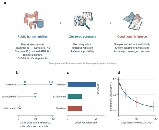
Figure 1. Study design and sampling observability. (a) Conceptual analysis workflow; perturbation sample sizes refer to antibiotic, environmental and diarrhea cohorts, respectively. The arrows indicate progression from public source profiles through observed contrasts to conditional inference. The longitudinal cohorts contain nine and 19 participants; a four-person metagenomic subset overlaps the former. Artwork in a is conceptual and does not represent measured results. (b) Representative positive post-peak times; open symbols mark the acute reference. The diarrhea example uses seven days and is not a common observed follow-up. (c) Local Jacobian rank with β fixed; two parameters are required. (d) An illustrative common law sampled at unequal times. Bars show illustrative central 95% Gaussian noise intervals (s.d. 0.06). This illustration is not fitted to the cohort data. Panel (d) is a hypothetical working model illustration and does not identify a biological recovery law.

3. Results

3.1. Sampling Schedules Determine Which Recovery Quantities Are Estimable

We examined three perturbation settings and two longitudinal comparison cohorts (Figure 1a; Table S1). The antibiotic analysis used 57 SPIRE v1 mOTUs3 profiles from 12 participants, retaining 643 features [2,19]. Sun supplied complete T0/T3/T6 triplets for 14 students, retaining 208 species and 412 ARG features. Boolchandani eligibility required the closest preTD sample, day 0 and earliest positive follow-up within 14 days from a distinct participant; 23 triplets had species profiles and 18 had complete ARG family profiles. Taxonomy excluded MF-prefixed resistance markers before filtering. BIO-ML required at least 30 distinct dated observations and negative recent antibiotic and GI infection screening fields, yielding 887 profiles aggregated into 802 person-days from nine donors and 321 ASVs. Vandeputte excluded three nonzero profiles without Day_Number and infection participant 808, yielding 672 RMP person-days from 19 people and 99 features.

Baseline and acute reference availability differed across datasets. Antibiotic D0, D8, D42 and D180 were observed in all 12 participants, while D4 was missing in three. Every primary Aitchison acute maximum was D8, leaving only two positive post-peak observations per person. Sun had one post-exposure observation approximately 90 days after T3, and each diarrheal episode had one follow-up within 14 days (Figure 1b). BIO-ML spans were 143–539 days; Vandeputte spans were 35–61 days. These observational cohorts had no defined perturbation or acute anchor. Same-day observations were aggregated before temporal feature selection. Missing dates and absent visits were excluded or retained as missing, never converted into zero abundance or interpolated. Nominal visits and actual dates remain separate in the released mappings.

We distinguished observed quantities, including within-person displacement and interval-specific distance ratios, from parameters requiring a recovery model. For the representative two-point antibiotic schedule, the prediction Jacobian had rank 2 with shape β fixed; the two one-point schedules had rank 1 (Figure 1c). Allowing β to vary left the antibiotic schedule with two constraints for three individual parameters. The actual primary antibiotic acute alignment likewise supplied only two positive time observations per participant (Table S8). Sampling one illustrative law at unequal follow-up times changed the observed ratios without changing its parameters (Figure 1d).

3.2. Antibiotic Exposure Is Followed by Partial Taxonomic Return with Uncertain Pooled Time Scales

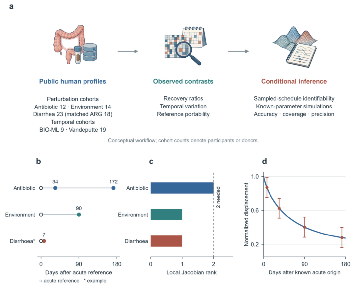
In the SPIRE reprocessing of Palleja, median Aitchison displacement was 2.383 at the observed acute maximum, 2.283 at D42 and 2.089 at D180 (Figure 2a). Nine of 12 participants had lower displacement at D42 than at the acute reference, and ten did so at D180. Median late-to-acute ratios were 0.945 at D42 (95% participant bootstrap CI 0.895–0.997; two-sided paired p = 0.0122, BH q = 0.0366) and 0.874 at D180 (0.810–0.992; p = 0.00684, q = 0.0246). Day-180 Jensen–Shannon and Bray–Curtis ratios were 0.768 and 0.707, respectively (Figure 2b; Table S2). These are within-participant contrasts against a sampled acute state, not tests of equivalence to baseline.

Figure 2. Antibiotic recovery in the SPIRE mOTUs3 reprocessing. (a) Aitchison displacement for 12 participants; thin lines are individual trajectories and the thick line joins visit medians. Visit positions are equally spaced for display. (b) Median late-to-observed-acute ratios with 20,000-draw participant bootstrap 95% intervals; circles denote D42 and squares D180. (c) Median D180 ratios under the observed maximum and fixed D8 references. (d) Conditional pooled τ estimates and 1000-draw participant cluster bootstrap intervals, on a logarithmic time axis, under nominal or calendar time and two fixed β values. These are pooled working model estimates, not individual recovery constants.

Acute reference selection depended on geometry. All primary Aitchison maxima occurred at D8, so replacing max (D4, D8) by a fixed D8 reference left the ratios unchanged. Five participants had D4 maxima under each alternative metric, changing the denominator and the time origin for subsequent observations (Figure 2c; Table S3). Agreement under Aitchison does not establish that D8 captured the biological peak.

Conditional pooled fits illustrate the distinction between fitting a curve and identifying individual dynamics. With shape fixed at β = 0.8 and nominal post-D8 times, participant-equal least squares gave τ = 65.5 days and residual displacement 0.873; the 1000-draw participant cluster bootstrap τ interval was 28.9–791.3 days. Calendar time gave τ = 55.5 days (29.1–472.8), while nominal time with β = 1 gave 50.9 days (29.2–141.9; Figure 2d; Table S4). The two nominal time models fit the same two group-level time coordinates equally well. D8 was a normalized reference in every primary trajectory and supplied no extra positive time observation. These shared parameter estimates concern this observed group; pooling does not identify each participant’s recovery scale or provide a cross-perturbation shape test.

3.3. Environmental Rebound Depends on Distance Metric; Early Diarrheal Follow-Up Does Not Establish Return

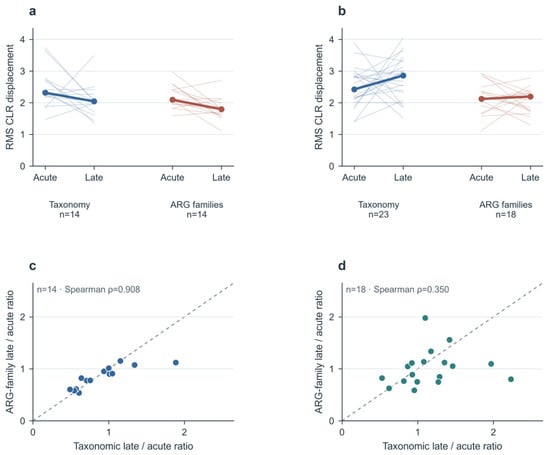
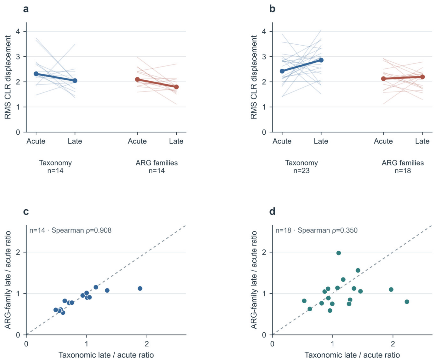
Environmental conclusions depended on how compositional change was measured (Figure 3a). Among these 14 participants, median species-level Aitchison displacement was 2.315 at T3 and 2.042 at T6. The median T6/T3 ratio was 0.846 (95% participant bootstrap CI 0.608–1.047), with nine ratios below one; the paired contrast was not significant (p = 0.153, BH q = 0.230). Jensen–Shannon and Bray–Curtis median ratios were 0.815 and 0.812, with p = 0.0166 and 0.0245 and q = 0.0427 and 0.0491. The environmental resistome Aitchison ratio was 0.862 (0.689–1.013; p = 0.0245, q = 0.0491). These metrics describe different aspects of the same profiles, rather than independent replications. The paired tests assess late-minus-acute distances, while the bootstrap intervals assess the median of participant ratios. Their different targets explain why a p value and a ratio interval need not cross their reference thresholds together (Table S2). We therefore describe metric-dependent evidence for partial rebound in this cohort.

Figure 3. Recovery contrasts and taxonomy–resistome association. (a,b), Individual Aitchison displacement at the acute reference and late follow-up for environmental exposure ((a) 14 participants per layer) and diarrhea ((b) 23 species profiles and 18 complete ARG family profiles). Thin lines connect each participant; thick lines join stage-specific medians. (c,d), Matched taxonomic and resistome recovery ratios for the environmental (c) and diarrhea (d) cohorts. Dashed lines denote equality and panel annotations report Spearman ρ. Diarrhea follow-up is the earliest eligible positive day, not necessarily a common day across participants. Associations are specific to these cohorts; shared reference error can contribute and no causal or universal coupling is inferred.

Follow-up after diarrhea was limited to the earliest eligible positive day within 14 days (Figure 3b). Across 23 participants, the species-only Aitchison late-to-acute ratio was 1.175 (95% participant bootstrap CI 0.954–1.298; two-sided p = 0.142, BH q = 0.230). Bray–Curtis and Jensen–Shannon medians were 1.099 and 1.122. Among 18 participants with complete ARG family profiles, the Aitchison resistome ratio was 0.968 (0.786–1.118; p = 0.417, q = 0.536). No diarrhea contrast remained significant after correction. Later recovery, complete return and persistent changes cannot be inferred from this short and heterogeneous follow-up.

3.4. Taxonomy–Resistome Association Is Supported After Environmental Exposure but Not After Diarrhea

Environmental taxonomic and resistome recovery ratios were positively associated under Aitchison geometry (Spearman ρ = 0.908; q = 4.38 × 10⁻⁵), Jensen–Shannon (ρ = 0.912; q = 4.38 × 10⁻⁵) and Bray–Curtis (ρ = 0.873; q = 1.87 × 10⁻⁴). Acute amplitudes were also associated (Aitchison ρ = 0.789; q = 0.00191). The species-only diarrhea analysis gave a weaker Aitchison ratio association among 18 matched participants (ρ = 0.350; p = 0.155; q = 0.206). Jensen–Shannon and Bray–Curtis ratio correlations were 0.288 and 0.135, respectively; none of the six diarrhea associations survived correction (Figure 3c,d and Table S5).

The environmental association is specific to the 14 analyzed participants, their profiles, reference states and observation window. It is not evidence for universal taxonomy–resistome coupling, and the diarrhea analysis did not provide statistically supported replication under the declared correction. Correlation of recovery ratios neither identifies a common time constant nor establishes a causal mechanism. Both layers share participants and baseline observations, so correlated measurement error and normalization can contribute to association. Separating resistance marker columns from taxonomy before preprocessing is essential to avoid comparing overlapping endpoints. ARG family composition, encoded metabolic pathways and biological activity are distinct properties and cannot be substituted for one another.

3.5. Participant-Level Compositional Differences Increase with Sampling Interval

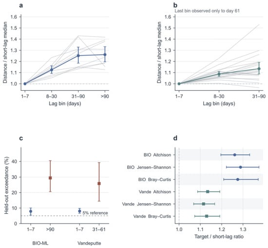
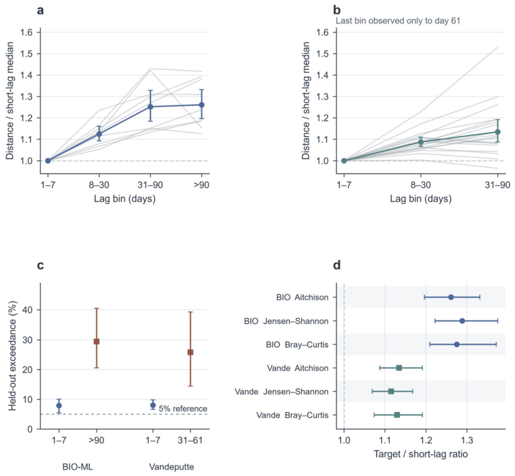
The primary BIO-ML set contained nine donors with 887 original 16S profiles, combined into 802 distinct person-days. The >90-day median Aitchison distance exceeded each donor’s own 1–7-day median in all nine donors. The participant-equal geometric mean of these ratios was 1.261 (95% participant bootstrap CI 1.196–1.332; exact two-sided signed-rank p = 0.00391, Holm q = 0.00391; Figure 4a). Jensen–Shannon and Bray–Curtis estimates were 1.288 and 1.275. In Vandeputte, excluding the documented infection in participant 808, the corresponding Aitchison ratio for the 31–90-day bin was 1.134 (1.088–1.192; p = 1.91 × 10⁻⁵, Holm q = 3.81 × 10⁻⁵), with 18 of 19 participants above one (Figure 4b). This bin contained only observed intervals up to 61 days. Distances and feature universes were not pooled across cohorts.

Figure 4. Participant-level temporal variation and blocked reference validation. (a,b) Individual ratios of median Aitchison distance in each lag bin to the same participant’s 1–7-day median (thin gray lines), with participant-equal geometric means and 20,000-draw participant bootstrap 95% intervals (BIO-ML, blue; Vandeputte, teal). In panel (c), circles indicate the 1–7-day reference lag and squares indicate the target lag; in panel (d), circles represent BIO-ML and squares represent Vandeputte. The reference bin equals one by definition. BIO-ML includes nine donors; Vandeputte includes 19 and has no lags beyond 61 days. (c) Participant mean held-out exceedance for short and target lags under alternating 14-day block validation; bars are participant bootstrap intervals. (d) Target-to-short ratios under three distance geometries. Pair counts are not inferential sample sizes; metagenomic and QMP sensitivities are reported separately.

Many sample pairs do not increase the number of independent participants. The primary BIO-ML result used 20,388 dependent long-lag date pairs but only nine biological replicates. Table S13 reports each participant’s effect and denominator. The overlapping four-person metagenomic subset gave a >90-day Aitchison ratio of 1.118 (1.083–1.171); it is a technical sensitivity, not independent replication. Restricting BIO-ML to its first 140 calendar days reduced the ratio to 1.151 (1.048–1.271), showing that observation coverage changes its magnitude. These interval-specific contrasts do not establish a monotonic trajectory for every person.

We assessed reference threshold portability separately using alternating 14-day calendar blocks. Both endpoints of an evaluated pair were held out from the short-lag pairs used to estimate its fold-specific 95th percentile. BIO-ML participant mean exceedance was 7.9% for held-out 1–7-day pairs and 29.4% for >90-day pairs; their paired difference was 21.5 percentage points (95% participant bootstrap CI 13.8–31.5). Corresponding Vandeputte values were 8.1%, 25.8% and 17.8 percentage points (7.0–30.6; Figure 4c). One BIO-ML fold had fewer than 20 training short pairs and was omitted, although all nine donors contributed to both reported bins. Dependence across neighboring blocks remains possible, and these are reference exceedance estimates rather than clinical false positive rates.

Robustness of Reference Portability

The positive lag contrast persisted with seven- and 21-day blocks, although the number of eligible contributors changed, particularly in Vandeputte. Target-minus-short differences also remained positive with 1- and 3-day training embargoes. A 7-day embargo retained four BIO-ML donors and one Vandeputte participant. The latter contrast was negative and is reported descriptively, without a population confidence interval (Figure S6; Table S19). These analyses assess reference portability within the available data; stronger temporal separation leaves too few contributors to establish independence or diagnostic performance.

Abundance representation also limited interpretation. In the matched 19-person QMP dataset, the closed composition Aitchison and Bray–Curtis ratios were 1.120 and 1.124. Bray–Curtis on unclosed absolute abundances gave 1.060 (0.999–1.133). Evidence was therefore clearer for relative composition than for absolute abundance. The original Vandeputte study found no clear similarity decay in its 36-day analysis [18]; our preprocessing and participant-weighted estimand differ and do not overturn that finding. Its observed spans of 35–61 days provide no >90-day comparison and cannot establish long-term stability or recovery after a perturbation. Figure S5 reports a separate sensitivity analysis for David Subject A.

3.6. Sparse Post-Peak Sampling Leaves Individual Recovery Parameters Unidentified

We evaluated local identifiability under the available sampling designs, rather than structural identifiability of a continuously observed model [24]. For the normalized family $r(t)=d_{\infty }+(1-d_{\infty }\left)\exp \right[-{(t/\tau )}^{\beta }]$, with τ > 0, β > 0 and 0 ≤ d_∞ < 1, one post-peak observation supplies one scalar constraint. With β fixed, compatible (τ, d_∞) values generally form a continuum; freeing β adds another unconstrained direction. At t = 0, the normalized response equals one for every admissible parameter set, so this point adds no information about the recovery parameters. Additional sequencing depth at the same time cannot supply a missing temporal constraint.

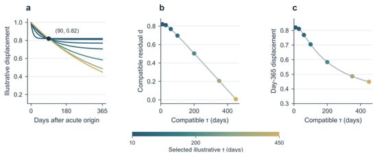
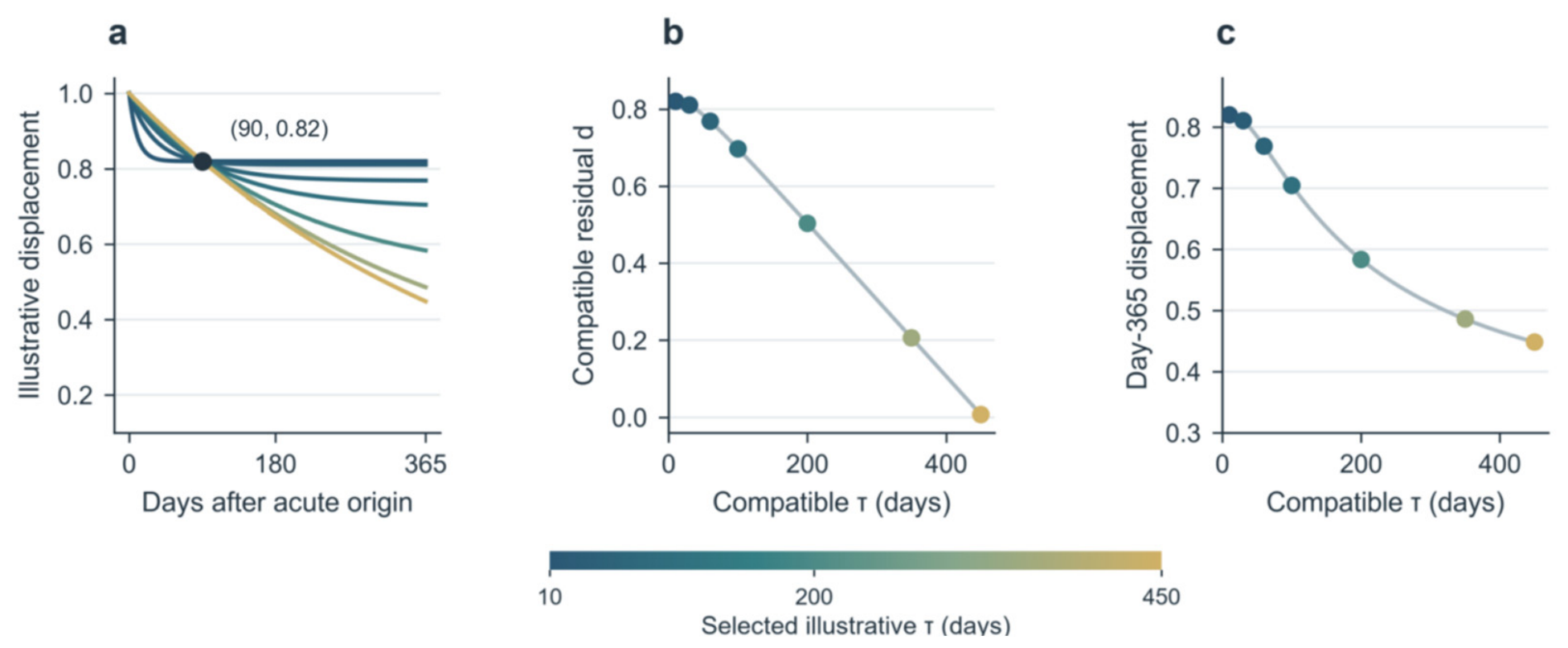
For illustration, r (90) = 0.82 with β = 1 is compatible with multiple recovery trajectories (Figure 5). This value is illustrative and is not the environmental Aitchison median. Within 0 ≤ d_∞ < 1, τ can range up to −90/ln(0.82) ≈ 453.5 days; predicted day-365 displacement ranges from approximately 0.447 to a limiting value of 0.82. At τ = 60 days, d_∞ = 0.2 and β = 0.8, and the representative antibiotic schedule (34, 172 days) has rank 2. Its two-norm condition number is 493.6 in coordinates (τ, d_∞) and 8.65 in (log τ, d_∞). Conditioning is coordinate-dependent, so the raw number alone cannot establish poor biological precision. With β free, rank remains 2 for three parameters and the full inverse problem is singular (Table S8).

Figure 5. One post-peak observation permits multiple recovery trajectories. (a) Seven illustrative exponential trajectories with r(90) = 0.82 and β = 1. (b) The admissible continuum of τ and d∞ values. (c) Different predictions at day 365 across the same parameter family. Colors identify the selected hypothetical τ values consistently across panels. The day-365 range is bounded but non-unique. These are analytical examples of sampling design non-identifiability, not fitted biological parameter estimates. The exponential family is used to demonstrate an inverse problem, not a validated biological mechanism.

Time scale normalization is a model-dependent inferential step. With two positive time points and fixed shape, two parameters may be locally identifiable in an ideal noiseless model, but residual variance cannot be estimated and practical precision can be poor. Allowing shape to vary leaves three individual parameters underdetermined. Estimating normalization parameters and judging collapse using the same data can obscure these uncertainties. An independent prediction task needs a normalization rule that excludes the outcomes being predicted, or an explicit hierarchical model that propagates normalization uncertainty. Pooling supplies shared parameter or distributional assumptions; it does not create the missing individual observations.

3.7. Preprocessing Sensitivities Preserve Cohort-Specific Contrasts

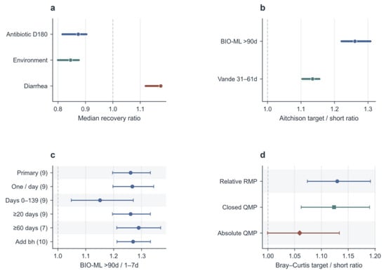
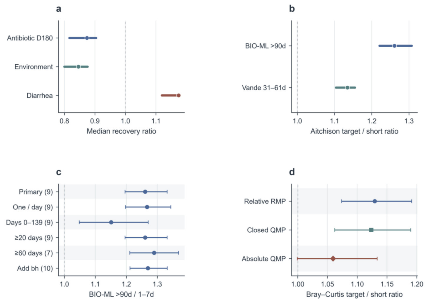
Preprocessing sensitivity preserved the direction of the primary relative composition contrasts without implying common recovery parameters. Across the nine prevalence and zero-replacement settings, the antibiotic D180 median ratios ranged from 0.816 to 0.904, environmental ratios from 0.800 to 0.876 and species-only diarrhea ratios from 1.119 to 1.175 (Figure 6a; Table S7). The BIO-ML long-to-short geometric mean ratios ranged from 1.221 to 1.307, and the Vandeputte target-to-short ratios from 1.104 to 1.155 (Figure 6b). Each participant leave-one-out estimate remained above one: 1.243–1.279 in BIO-ML and 1.116–1.145 in Vandeputte. These are sensitivity ranges, not independent replications or additional confirmatory tests.

Figure 6. Sensitivities delimit the scope of inference. (a) Primary median recovery ratios and ranges across nine prevalence/zero-replacement settings for antibiotic D180, environmental follow-up and diarrhea follow-up. (b) Corresponding preprocessing ranges for the two primary Aitchison lag contrasts; bars in (a,b) show setting ranges, not confidence intervals. (c) BIO-ML analysis set sensitivities with participant bootstrap 95% intervals; parentheses give participant counts. (d) Vandeputte Bray–Curtis target-to-short ratios using relative profiles, closed QMP and unclosed absolute QMP. In panel (d), circles, squares and diamonds denote relative RMP, closed QMP and absolute QMP, respectively. Panels (c,d) use 20,000 participant bootstrap draws; sample pair counts do not determine these intervals.

Using one deterministically selected profile per BIO-ML day gave an Aitchison ratio of 1.267 (1.197–1.344). Requiring at least 60 unique days retained seven donors and gave 1.290 (1.211–1.369); including the flagged donor bh gave 1.270 (1.212–1.332; Figure 6c). The sensitivity windows are defined explicitly in Table S14: elapsed days 0–139 for BIO-ML and recorded Day_Number ≤ 36 for Vandeputte. Their results depend on the stated window and refitted feature universe, rather than being independent replications. Participant and 14-day block deletion analyses assess the influence of individual contributors and observation periods. Absolute QMP contrasts were weaker than relative composition contrasts (Figure 6d), and no sensitivity establishes an individual universal recovery curve.

3.8. Known Parameter Simulations Quantify Timing Gains and Limits of Uncertainty Calibration

We simulated scalar recovery trajectories with specified τ = 10, 30 or 90 days, residual displacement 0.20, 0.60 or 0.85, fitted shape β = 1 and independent Gaussian noise of standard deviation 0.03 or 0.08. Nine schedules supplied two, three, six, nine or 12 positive post-peak observations, with 2000 repetitions in each of 162 primary schedule–truth cells. Common date noise vectors paired schedule comparisons within each repetition. Separate experiments changed the shape, serial dependence and noisy acute references (Figure 7a; Table S15). These hypothetical ranges span fast/slow and strong/weak signal regimes; they were not estimated from the sparse cohort trajectories and do not represent simulated biological participants.

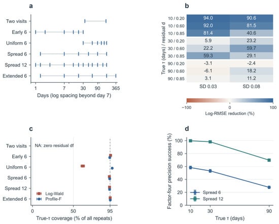
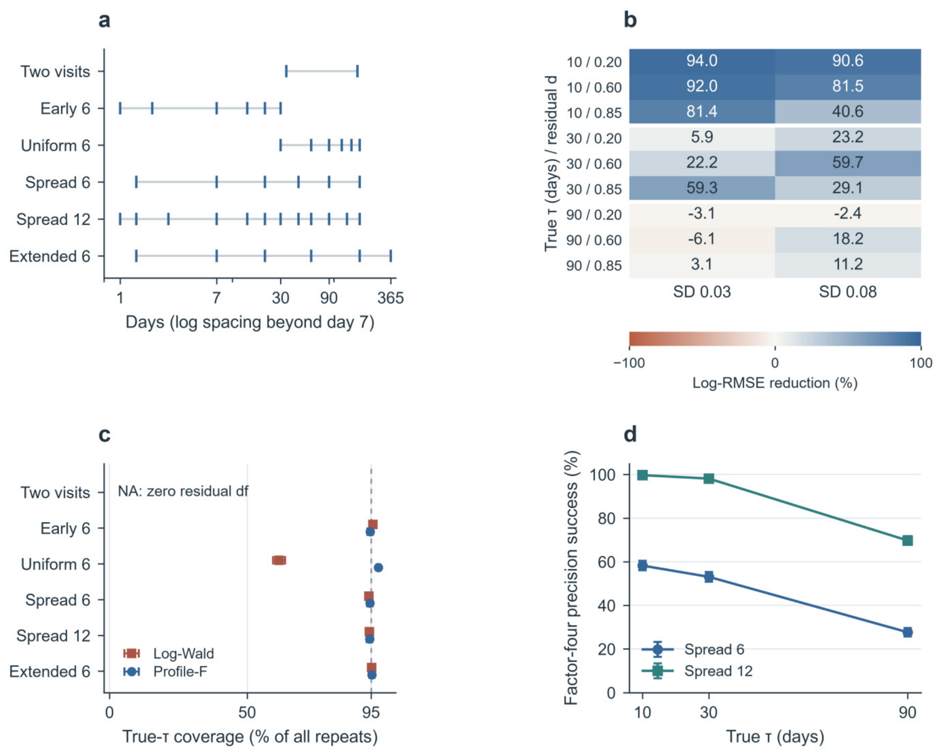
Figure 7. Sampling design affects accuracy, coverage and precision in simulations. (a) Selected follow-up schedules, in days after a known acute origin; spacing is logarithmic beyond day 7. The primary experiment uses an exact acute reference. (b) Percentage reduction in root mean squared log(estimated τ/true τ) for spread six relative to uniform six across all 18 primary parameter combinations. Negative values indicate worse performance; the color scale is centered at zero. (c) Coverage of log-Wald t intervals and profile-F sets at τ = 10 days, residual 0.20 and independent Gaussian noise s.d. 0.08. (d) Probability of a bounded profile set envelope with upper/lower ratio ≤ 4 at residual 0.20 and s.d. 0.08. Bars in (c,d) are ±1.96 Monte Carlo standard errors across 2000 repetitions. All-repeat coverage counts unavailable intervals as unsuccessful. Two-visit intervals are unavailable (NA) because residual degrees of freedom are zero. Coverage and envelope width are separate outcomes. The generating parameters define hypothetical scalar scenarios; repetition counts and uncertainty bars do not describe a human population.

Timing gains depended on the scenario. At τ = 10 days, residual 0.20 and noise standard deviation 0.08, spread six sampling at days 2, 7, 21, 45, 90 and 180 reduced log-scale τ RMSE by 90.6% relative to uniform six sampling at days 30, 60, 90, 120, 150 and 180 (paired Monte Carlo standard error 0.2 percentage points). Estimates within 25% of truth increased from 25.4% to 69.0% (Figure 7b; Table S16). For true τ = 10 days, that accuracy criterion means an estimate between 7.5 and 12.5 days. The log-RMSE gain varied from 82.0% to 93.7% under the alternative search bounds. At τ = 90 days with the same residual and noise, spread six had 2.4% higher log-RMSE than uniform six. Extending six visits to day 365 reduced log-RMSE by 17.7% relative to spread six (Monte Carlo standard error 1.6 percentage points). None of these schedules was universally best.

Restricting follow-up also affected point estimates and extrapolation. At τ = 30 days, residual 0.85 and noise standard deviation 0.08, six visits restricted to days 1–30 gave a median relative τ error −44.5%, compared with −14.8% under spread six. Mean residual error was −0.270 versus −0.099, and day-365 displacement prediction RMSE was 0.365 versus 0.100 (Figure S7). Mean τ error is particularly sensitive to long estimator tails and search bounds, so mean and median errors are reported alongside log-RMSE, fit failures and boundary diagnostics. A point estimate on a numerically flat profile may have little practical precision.

Coverage, interval availability and useful precision were different outcomes. In the fast scenario, log-Wald intervals covered truth in 61.6% of all uniform six repetitions; 647 of 2000 repeats had no usable full-rank Wald interval. Coverage among available Wald intervals was 91.1%. Profile F sets covered truth in 97.7% of all repeats, but only 5.3% had bounded envelopes. Spread six gave 94.5% profile coverage and 99.8% bounded envelopes. The two-visit design has zero residual degrees of freedom and no estimated variance interval. Increasing spread six to spread twelve reduced log-RMSE by 15.6–34.6% across the 18 primary scenarios. At τ = 10 days, residual 0.20 and noise 0.08, factor four precision increased from 58.2% to 99.7%. At residual 0.85, it was only 0.0–0.1% despite 12 visits. Factor four is this study’s planning threshold, not a biological or clinical standard (Figure 7c,d).

More observations did not repair model misspecification. When true β was 0.7 but fitted β remained 1, spread twelve at τ = 90 days, residual 0.20 and noise 0.08 gave a median τ error −46.8%, exact set coverage 61.6% and factor four precision 46.8%. Thus, many narrow sets still missed truth. With 14-day correlated errors, spread twelve coverage ranged from 72.5% to 88.8% across the four stress combinations (Figure S8; Table S17). With three noisy acute observations, τ = 30 days, residual 0.85 and noise 0.08, acute maximum normalization gave a median error −61.9% and coverage 84.0%. Acute mean normalization gave −5.5% and 95.5%; joint raw fitting gave −8.5% and 96.4%. Joint fitting met the precision criterion in 0.0% of this weak signal scenario. Mean normalization and joint fitting reduced the maximum selection distortion here, without guaranteeing precision or solving unknown biological peak timing (Figure S9; Table S18).

4. Discussion

The empirical findings are conditional on the cohorts and observation windows analyzed. Antibiotic profiles supported reduced displacement from the sampled acute reference, whereas environmental evidence varied by metric and early diarrhea follow-up was inconclusive. Taxonomy–resistome ratios were associated in the environmental cohort but not convincingly in the diarrhea cohort. The longitudinal comparisons concerned interval-dependent relative composition in nine BIO-ML and 19 Vandeputte participants. These results do not establish universal coupling, complete recovery or a common recovery law. Their sample pair counts cannot compensate for limited biological replication.

The simulations show how observation times affect parameter estimation under a specified model. Early measurements were useful when recovery was fast, whereas later follow-up helped distinguish slow change from residual displacement. The size of these gains depended on the generating time scale, shape, signal and error structure; some conventional schedules performed as well as or better than spread six. Interval coverage and precision also differed. A procedure could include the true value frequently while producing intervals too wide for a useful estimate. These results inform the evaluation of sampling designs under stated assumptions and do not identify the biological trajectories of the analyzed cohorts.

The cohort summaries and individual inverse problems answer different questions. A participant-weighted contrast or median trajectory can reveal a group pattern while individuals remain heterogeneous. Pooling can estimate common parameters only after assuming that participants share the stated curve, time scale or residual state; hierarchical models would introduce a specified distribution and borrowing rule. Neither approach creates additional observed time points for an individual. With two positive post-peak observations and three free individual parameters, the unconstrained individual problem remains underdetermined. A visually aligned group curve therefore cannot demonstrate a universal individual recovery trajectory.

4.1. How Acute References Affect Recovery Inference

Two distinct acute reference errors can act in opposite directions. Let A* be the true maximum displacement from a fixed baseline and Aobs the largest noiseless sampled displacement, with 0 < Aobs ≤ A*. For the same late displacement L, the observed ratio L/Aobs is at least L/A*. Missing the peak can therefore make apparent return weaker. For illustration, if Aobs is 80% of A*, the observed ratio is 25% larger than the true peak ratio. This is an algebraic sensitivity calculation, not an estimated bias in any cohort. In contrast, choosing the maximum of noisy acute measurements can inflate the denominator and make apparent return stronger. Baseline noise, non-monotonic dynamics and a changed acute time origin complicate the net effect. Supplementary Methods S14 separates these mechanisms.

A missed peak also changes the elapsed time from the true peak, so the direction of bias in a fitted τ or residual state cannot be inferred from the ratio inequality alone. Our acute replicate experiment evaluates maximum selection at one known origin; it does not quantify actual missed peak timing. Future designs should sample around a plausible acute window, preserve all acute observations, retain calendar times and assess sensitivity to the reference and time origin. A fixed D8 comparison is useful but cannot confirm that a continuous peak was captured.

4.2. Interpretation Limits and Study Planning

Temporal variation raises a separate reference calibration problem [1,5,14,26]. Endpoint disjoint block validation protects against reusing the same samples in reference and evaluation pairs, but neighboring blocks can remain correlated. Changing the block length and deleting participants or periods assess sensitivity; they do not prove temporal independence. Training embargoes of 1, 3 and 7 days further separate reference endpoints from held-out observations (Figure S6; Table S19). The 1- and 3-day embargo contrasts remained positive in both cohorts, although Vandeputte retained only 14 contributors at 3 days. At 7 days, valid target comparisons fell to four BIO-ML donors and one Vandeputte participant. The latter gave a descriptive negative contrast with no population interval. Stronger isolation therefore exposes a data limitation, rather than establishing robustness at every separation. These exceedances concern the portability of a reference quantile, not a clinical false positive rate.

Relative and absolute abundance support different interpretations. Closure removes total abundance, so a return in relative composition does not demonstrate the restoration of microbial load. The weaker absolute QMP result is compatible with the original Vandeputte report and limits the interpretation of the lag contrast [18]. ARG family composition, pathway potential and measured activity also represent different biological properties. Functional profiles matched to the SPIRE taxonomic processing were unavailable, preventing a comparison of pathway and taxonomic recovery slopes.

Several limitations restrict generalization. Cohorts were small and not population-representative; screening fields do not exclude every later illness, treatment or exposure. Metagenomic and QMP subsets overlap the primary cohorts. Same-day samples are not verified technical replicates. Participant bootstrap intervals assume independent, exchangeable participants for the cohort-level estimand, resample their complete observed trajectories, and condition on their sampling calendars and processed profiles. They preserve temporal structure but do not generate unobserved within-person trajectories or fully propagate measurement and preprocessing uncertainty. Small participant counts can limit percentile interval calibration. Vandeputte has no observations beyond 61 days and the diarrhea endpoint is within 14 days, so neither establishes long-term or complete post-perturbation recovery. The analysis used study-specific released profiles without a common raw read processing pipeline, and signed-rank inference assumes symmetric participant-level differences.

The simulations assume a known acute origin and monotone noiseless return to a residual state between zero and one. The working model cannot represent all observed overshoots, recurrent perturbations or increases in late displacement. The selected time scales span illustrative regimes and the residual/noise combinations alter observable signal-to-noise; they were not calibrated to a biological population. Fixed β = 1 is an estimation assumption, while 0.7 and 1.3 are stress scenarios. Additive Gaussian noise permits negative scalar observations and does not generate taxa or sequencing counts. Joint raw fitting assumes homogeneous independent errors and the same true amplitude at repeated acute observations. Numerical rank and boundary checks help assess this implementation; they do not validate a biological mechanism or establish a sufficient sample count when shape, baseline, peak time and covariance must also be estimated.

Study planning should begin with the biological question and observable endpoint. A displacement ratio, equivalence to an individual baseline range and a model-based time scale are different targets. Define the primary metric, baseline, acute window rule, analysis unit and multiplicity family before evaluating recovery. Obtain repeated pre-event observations, retain raw acute measurements and record actual collection times and relevant exposures. The required numbers of baseline or acute samples were not established here. Table 2 summarizes the planning implications, with assumptions and limitations detailed in Supplementary Methods S13–S15.

Table 2. Conditional design and analysis guidance.

Design Question	Candidate Action	Evidence and Boundary
What should recovery mean?	Prespecify the primary distance, sampled time contrast, baseline range and clinical or functional endpoint.	Ratio < 1 means less displacement than the sampled acute reference. Complete return needs a separate equivalence definition.
How should baseline and acute states be observed?	Obtain repeated pre-event observations where feasible; sample around the plausible acute window and retain all raw profiles and actual times.	These are design considerations. This study does not determine a sufficient baseline or acute sample count.
Could the recovery scale be 10–30 days?	Evaluate follow-ups at days 2, 7, 21, 45, 90 and 180.	Candidate under the tested fixed-shape scalar model and known acute origin; not a validated biological schedule.
Could recovery extend towards 90 days?	Evaluate days 2, 7, 21, 60, 180 and 365.	Extending the tail can help in the tested slow scenarios; use feasible biological event times and assess loss to follow-up.
Is greater model precision required?	Evaluate the 12 follow-ups in Table S15 and prespecify acceptable bias, coverage and interval width.	More visits can help, but high residual displacement or weak signal can leave even 12 visits uninformative.
Are shape, errors or peak timing uncertain?	Stress test plausible shapes, noise, serial dependence and reference rules before committing visits.	The tested exponential family is a working model. Joint raw fitting does not solve unknown peak time or baseline noise.
How should inference be reported?	Resample whole participants; report the effect, interval, number of participants, observation window, metric sensitivity and model limitations.	Sample pairs are dependent. Validate predictions independently of fitting and normalization.

5. Conclusions

Observed recovery contrasts depend on the cohort, reference state and distance metric, while relative composition differences vary with the interval between samples. Under the tested models, observation timing and acute reference handling affect the accuracy and precision of recovery-scale estimates. Sampling designs should therefore be evaluated against explicit targets for accuracy, coverage and interval width. The available data do not establish a universal recovery law across perturbations.

References

- Lozupone, C.A.; Stombaugh, J.I.; Gordon, J.I.; Jansson, J.K.; Knight, R. Diversity, stability and resilience of the human gut microbiota. Nature 2012, 489, 220–230. [Google Scholar] [CrossRef] [Scilit] [PubMed]
- Palleja, A.; Mikkelsen, K.H.; Forslund, S.K.; Kashani, A.; Allin, K.H.; Nielsen, T.; Hansen, T.H.; Liang, S.; Feng, Q.; Zhang, C.; et al. Recovery of gut microbiota of healthy adults following antibiotic exposure. Nat. Microbiol. 2018, 3, 1255–1265. [Google Scholar] [CrossRef] [Scilit] [PubMed]
- Sun, J.; Liao, X.P.; D’Souza, A.W.; Boolchandani, M.; Li, S.H.; Cheng, K.; Martínez, J.L.; Li, L.; Feng, Y.J.; Fang, L.X.; et al. Environmental remodeling of human gut microbiota and antibiotic resistome in livestock farms. Nat. Commun. 2020, 11, 1427. [Google Scholar] [CrossRef] [Scilit] [PubMed]
- Boolchandani, M.; Blake, K.S.; Tilley, D.H.; Cabada, M.M.; Schwartz, D.J.; Patel, S.; Morales, M.L.; Meza, R.; Soto, G.; Isidean, S.D.; et al. Impact of international travel and diarrhea on gut microbiome and resistome dynamics. Nat. Commun. 2022, 13, 7485. [Google Scholar] [CrossRef] [Scilit] [PubMed]
- David, L.A.; Materna, A.C.; Friedman, J.; Campos-Baptista, M.I.; Blackburn, M.C.; Perrotta, A.; Erdman, S.E.; Alm, E.J. Host lifestyle affects human microbiota on daily timescales. Genome Biol. 2014, 15, R89, Erratum in Genome Biol. 2016, 17, 117. [Google Scholar] [CrossRef] [Scilit] [PubMed]
- von Schwartzenberg, R.J.; Bisanz, J.E.; Lyalina, S.; Spanogiannopoulos, P.; Ang, Q.Y.; Cai, J.; Dickmann, S.; Friedrich, M.; Liu, S.Y.; Collins, S.L.; et al. Caloric restriction disrupts the microbiota and colonization resistance. Nature 2021, 595, 272–277. [Google Scholar] [CrossRef] [Scilit] [PubMed]
- Hansen, Z.A.; Vasco, K.; Rudrik, J.T.; Scribner, K.T.; Zhang, L.; Manning, S.D. Recovery of the gut microbiome following enteric infection and persistence of antimicrobial resistance genes in specific microbial hosts. Sci. Rep. 2023, 13, 15524. [Google Scholar] [CrossRef] [Scilit] [PubMed]
- Shaw, L.P.; Bassam, H.; Barnes, C.P.; Walker, A.S.; Klein, N.; Balloux, F. Modelling microbiome recovery after antibiotics using a stability landscape framework. ISME J. 2019, 13, 1845–1856. [Google Scholar] [CrossRef] [Scilit] [PubMed]
- Chng, K.R.; Ghosh, T.S.; Tan, Y.H.; Nandi, T.; Lee, I.R.; Ng, A.H.Q.; Li, C.; Ravikrishnan, A.; Lim, K.M.; Lye, D.; et al. Metagenome-wide association analysis identifies microbial determinants of post-antibiotic ecological recovery in the gut. Nat. Ecol. Evol. 2020, 4, 1256–1267. [Google Scholar] [CrossRef] [Scilit] [PubMed]
- Anthony, W.E.; Wang, B.; Sukhum, K.V.; D’Souza, A.W.; Hink, T.; Cass, C.; Seiler, S.; Reske, K.A.; Coon, C.; Dubberke, E.R.; et al. Acute and persistent effects of commonly used antibiotics on the gut microbiome and resistome in healthy adults. Cell Rep. 2022, 39, 110649. [Google Scholar] [CrossRef] [Scilit] [PubMed]
- d’Humières, C.; Delavy, M.; Alla, L.; Ichou, F.; Gauliard, E.; Ghozlane, A.; Levenez, F.; Galleron, N.; Quinquis, B.; Pons, N.; et al. Perturbation and resilience of the gut microbiome up to 3 months after β-lactams exposure in healthy volunteers suggest an important role of microbial β-lactamases. Microbiome 2024, 12, 50. [Google Scholar] [CrossRef] [Scilit] [PubMed]
- Baldanzi, G.; Larsson, A.; Sayols-Baixeras, S.; Dekkers, K.F.; Hammar, U.; Nguyen, D.; Graells, T.; Ahmad, S.; Gazolla Volpiano, C.; Meric, G.; et al. Antibiotic use and gut microbiome composition links from individual-level prescription data of 14,979 individuals. Nat. Med. 2026, 32, 1351–1361. [Google Scholar] [CrossRef] [Scilit] [PubMed]
- Bashan, A.; Gibson, T.E.; Friedman, J.; Carey, V.J.; Weiss, S.T.; Hohmann, E.L.; Liu, Y.Y. Universality of human microbial dynamics. Nature 2016, 534, 259–262. [Google Scholar] [CrossRef] [Scilit] [PubMed]
- Shoemaker, W.R.; Grilli, J. The macroecological dynamics of sojourn trajectories in the human gut microbiome. mSystems 2026, 11, e01221-25. [Google Scholar] [CrossRef] [Scilit] [PubMed]
- Aitchison, J. The Statistical Analysis of Compositional Data; Chapman and Hall: London, UK, 1986. [Google Scholar]
- Gloor, G.B.; Macklaim, J.M.; Pawlowsky-Glahn, V.; Egozcue, J.J. Microbiome datasets are compositional: And this is not optional. Front. Microbiol. 2017, 8, 2224. [Google Scholar] [CrossRef] [Scilit] [PubMed]
- Poyet, M.; Groussin, M.; Gibbons, S.M.; Avila-Pacheco, J.; Jiang, X.; Kearney, S.M.; Perrotta, A.R.; Berdy, B.; Zhao, S.; Lieberman, T.D.; et al. A library of human gut bacterial isolates paired with longitudinal multiomics data enables mechanistic microbiome research. Nat. Med. 2019, 25, 1442–1452. [Google Scholar] [CrossRef] [Scilit] [PubMed]
- Vandeputte, D.; De Commer, L.; Tito, R.Y.; Kathagen, G.; Sabino, J.; Vermeire, S.; Faust, K.; Raes, J. Temporal variability in quantitative human gut microbiome profiles and implications for clinical research. Nat. Commun. 2021, 12, 6740. [Google Scholar] [CrossRef] [Scilit] [PubMed]
- SPIRE. Palleja 2018 Antibiotics SPIRE v1 mOTUs3 Profiles. Available online: https://spire.embl.de/spire/v1/study/Palleja_2018_antibiotics (accessed on 14 October 2026).
- Gibbons Laboratory. BIO-ML Species Counts and Associated Metadata. Available online: https://github.com/Gibbons-Lab/human-microbiome-time-series-growth-phase-estimation (accessed on 14 October 2026).
- Faust, K.; Bauchinger, F.; Laroche, B.; de Buyl, S.; Lahti, L.; Washburne, A.D.; Gonze, D.; Widder, S. Signatures of ecological processes in microbial community time series. Microbiome 2018, 6, 120. [Google Scholar] [CrossRef] [Scilit] [PubMed]
- Benjamini, Y.; Hochberg, Y. Controlling the false discovery rate: A practical and powerful approach to multiple testing. J. R. Stat. Soc. B 1995, 57, 289–300. [Google Scholar] [CrossRef] [Scilit]
- Morris, T.P.; White, I.R.; Crowther, M.J. Using simulation studies to evaluate statistical methods. Stat. Med. 2019, 38, 2074–2102. [Google Scholar] [CrossRef] [Scilit] [PubMed]
- Raue, A.; Kreutz, C.; Maiwald, T.; Bachmann, J.; Schilling, M.; Klingmüller, U.; Timmer, J. Structural and practical identifiability analysis of partially observed dynamical models by exploiting the profile likelihood. Bioinformatics 2009, 25, 1923–1929. [Google Scholar] [CrossRef] [Scilit] [PubMed]
- Bates, D.M.; Watts, D.G. Nonlinear Regression Analysis and Its Applications; Wiley: New York, NY, USA, 1988. [Google Scholar] [CrossRef] [Scilit]
- Procházková, N.; Laursen, M.F.; La Barbera, G.; Tsekitsidi, E.; Jørgensen, M.S.; Rasmussen, M.A.; Raes, J.; Licht, T.R.; Dragsted, L.O.; Roager, H.M. Gut physiology and environment explain variations in human gut microbiome composition and metabolism. Nat. Microbiol. 2024, 9, 3210–3225. [Google Scholar] [CrossRef] [Scilit] [PubMed]
Disclaimer/Publisher’s Note: The statements, opinions and data contained in all publications are solely those of the individual author(s) and contributor(s) and not of MDPI and/or the editor(s). MDPI and/or the editor(s) disclaim responsibility for any injury to people or property resulting from any ideas, methods, instructions or products referred to in the content. |
© 2026 by the authors. Licensee MDPI, Basel, Switzerland. This article is an open access article distributed under the terms and conditions of the Creative Commons Attribution (CC BY) license.