


Abstract
Automated Guided Vehicles (AGVs) play a crucial role in intelligent warehousing; however, effective path planning remains challenging because of obstacles, safety constraints, and the risk of suboptimal routes. This study proposes an improved Harris Hawks Optimization algorithm for AGV path planning, introducing strategies to enhance initial solution quality, balance global and local search, and avoid local optima. The proposed algorithm generates shorter, smoother, and safer paths, as demonstrated through benchmark tests, multi-scale grid-map simulations, and real-world AGV experiments. In terms of path length and computational efficiency, the enhanced algorithm significantly outperforms the original HHO, reducing average path length by 10.81% and average travel time by 11.94%. These results demonstrate that the proposed method provides a practical and reliable solution for autonomous warehouse navigation and significantly improves AGV path-planning performance.
1. Introduction
With the rapid advancement of artificial intelligence, the Internet of Things, and automation technologies, intelligent mobile platforms have been widely adopted across various domains of production and daily life. Driven by the dual forces of e-commerce and intelligent manufacturing, modern warehouse logistics systems are undergoing profound transformation. As core actuators in smart warehousing, Automated Guided Vehicles (AGVs) have largely replaced manual labor in contexts such as high-bay warehouses, distribution centers, and intelligent production lines, undertaking critical tasks, including pallet handling, order picking, and cross-docking. In such environments, hundreds of AGVs are required to operate collaboratively in complex scenarios characterized by narrow aisles, densely arranged racks, and dynamically interwoven tasks. Their path-planning capability directly determines the system’s throughput efficiency. Therefore, rapidly generating short, smooth, and reliable collision-free paths for many AGVs has become a critical bottleneck, limiting improvements in warehousing efficiency. This challenge also reflects a common issue faced by intelligent agents such as autonomous vehicles and drones operating in dynamic and uncertain environments. These systems must not only perceive the environment but also understand it and generate feasible motion paths efficiently and safely.
Path-planning technology has emerged precisely to address this core challenge, aiming to identify a collision-free trajectory for AGVs from a starting point to a destination within a given warehousing environment, while achieving comprehensive optimization across multiple criteria such as path length, travel time, and energy consumption. As a core algorithm enabling autonomous AGV navigation, path-planning technology has evolved over years of development into a complete spectrum, ranging from classical deterministic methods to modern metaheuristic algorithms. Representative classical algorithms include the Dijkstra Algorithm [1], A-Star Algorithm [2], Genetic Algorithm (GA) [3], and Artificial Potential Field (APF) [4]. These algorithms perform well in structured environments: Dijkstra guarantees finding the shortest path from a start node to all other nodes in a weighted graph, albeit with extensive computational scope and relatively low efficiency; A-Star introduces a heuristic function to guide the search direction and has be-come one of the most widely applied algorithms in global path planning; APF treats the target as an attractive force and obstacles as repulsive forces, offering a simple structure and strong real-time performance, yet it is prone to becoming trapped in local optima in complex environments.
To further improve path-planning performance in practical warehousing and autonomous navigation scenarios, numerous studies have recently focused on AGV and autonomous mobile robot path-planning problems. As modern large-scale warehousing systems exhibit complex characteristics such as high dimensionality, multiple constraints, and strong nonlinearity, classical algorithms have gradually revealed limitations when applied to such problems, including high computational complexity, susceptibility to local optima, and low efficiency in solution space search. To overcome these shortcomings, researchers have proposed various improvement strategies for traditional path-planning algorithms. For example, Elias Xidias et al. [5] contributed a novel 3D Bump-Surface concept combined with a modified Genetic Algorithm to simultaneously solve path-planning and task scheduling problems for a fleet of autonomous vehicles in indoor factory environments, optimizing safety, time, and energy consumption. Furthermore, recent review studies have systematically summarized classical and heuristic-based autonomous mobile robot path-planning methods [6]. Nevertheless, traditional, heuristic methods still suffer from limitations in complex, high-dimensional, and nonlinear environments. Consequently, researchers have increasingly turned to metaheuristic and swarm intelligence optimization algorithms. These algorithms do not rely on gradient information, possess powerful global exploration and local exploitation capabilities, and can effectively address complex non-convex and nonlinear optimization problems. For instance, Nan, Yujie et al. proposed a multi-UAV path-planning algorithm based on an improved ant colony system (PS-ACO-SA) [7], which integrates ant colony optimization with particle swarm optimization and simulated annealing to address obstacle avoidance path planning for multiple UAVs in complex mountainous environments. Cheng, Qing et al. introduced GS-PSO [8], a novel multi-stage hybrid framework designed to solve the complex three-dimensional path-planning problem for UAV deployment in constrained environments by sequentially integrating particle swarm optimization (PSO), sparrow search algorithm (SSA), and Genetic Algorithm (GA). Liu, Y. [9] developed an improved ant colony optimization-based global path-planning method for warehousing AGVs, demonstrating enhanced transportation efficiency and environmental adaptability in complex logistics scenarios. In addition, Fan Ye et al. [10] proposed a hybrid artificial bee colony algorithm integrated with a genetic augmented exploration mechanism to improve path safety, smoothness, and optimization capability for mobile robot navigation. These studies demonstrate that metaheuristic algorithms not only transcend the inherent limitations of traditional methods but also facilitate multi-objective collaborative optimization, thereby expanding the methodological framework of path planning and establishing themselves as an important research direction in this field.
Among numerous metaheuristic algorithms, a class of emerging algorithms inspired by predatory behavior simulates the efficient hunting strategies of top predators, demonstrating an excellent balance between global and local search capabilities, making them particularly suitable for complex optimization problems, such as AGV path planning, which are high-dimensional and multimodal. For example, Grey Wolf Optimizer (GWO) [11] simulates social hierarchy and encircling mechanisms, Whale Optimization Algorithm (WOA) [12] mimics bubble-net hunting behavior, and Harris Hawks Optimization (HHO) models the strategies of surprise pounce, encirclement, and pursuit in cooperative hunting among hawks. Proposed by Heidari et al. in 2019 [13], HHO leverages an “exploration–transition–exploitation” mechanism that enables dynamic strategy adjustment based on the prey’s state, endowing it with exceptional global search capability and dynamic encircling ability that are particularly well-suited for solving multimodal, combinatorial, and nonlinear problems in path planning. Consequently, numerous researchers have applied HHO to domains related to path planning. However, when applied to high-dimensional and multi-constraint practical scenarios, the original HHO algorithm still encounters several limitations, including insufficient initial population quality, reduced exploration capability in complex obstacle environments, and unstable local search behavior during later iterations. These issues may lead to premature convergence and difficulty in generating globally optimal and smooth trajectories. To enhance the performance of HHO in path-planning applications, different improvement strategies have been investigated in recent studies. Some works focus on enhancing trajectory optimization efficiency through mathematical modeling and interpolation strategies, such as the seventh-degree polynomial interpolation-based IHHO proposed by Xu Jing et al. [14]. Other studies combine HHO with biologically inspired or neural-network-based mechanisms to improve search adaptability in complex environments, including the BINN-HHO framework developed by Li Sen et al. [15] for multi-UAV path planning. Chaotic search strategies and regression-based optimization mechanisms have also been incorporated into HHO to strengthen global exploration and avoid local optima in complex terrains [16]. In addition, hybrid optimization frameworks integrating HHO with other swarm intelligence algorithms, such as HHO-AVOA [17], have been employed to improve navigation performance for wheeled mobile robots in dynamic environments. Furthermore, multidimensional mission-space modeling and path–cost optimization methods have been introduced to extend HHO-based approaches to three-dimensional UAV path-planning problems [18].
Nevertheless, existing improvements still share some common limitations. Certain approaches rely on complex hybrid mechanisms, which increase algorithmic complexity while undermining the inherent advantage of HHO’s structural simplicity. Improvements to core parameters such as the energy factor tend to be relatively simplistic, making it difficult to effectively balance global exploration and local exploitation. Moreover, some strategies fail to achieve deep synergy with HHO’s unique mechanisms, thereby compromising the effectiveness of escaping local optima. And, in terms of application, most existing approaches mainly focus on benchmark optimization problems and lack sufficient validation in practical AGV path-planning environments. In addition, the balance between computational efficiency and path quality in warehouse scenarios remains insufficiently discussed.
Based on the above analysis, this paper aims to systematically investigate the application of the Harris Hawks Optimization (HHO) algorithm to path planning problems. To address the shortcomings of the standard algorithm and consider the complex characteristics of path-planning problems, such as multimodality, high dimensionality, and strong nonlinearity, an Enhanced Harris Hawks Optimization (EHHO) algorithm is proposed. Compared with existing AGV and mobile robot path-planning approaches, particularly HHO-based optimization methods, the proposed EHHO algorithm simultaneously considers population diversity, convergence stability, and local optimum avoidance for grid-based AGV path planning. Furthermore, the proposed method is evaluated not only on CEC2022 benchmark functions but also in warehouse grid map simulations and real-world AGV experiments to verify its practical applicability and optimization effectiveness. The main contributions of this paper are as follows:
- Mathematical Modeling for AGV Path Planning: A multi-objective optimization model is established for grid-based warehouse environments, considering path length, safety, and smoothness. This provides a structured framework for subsequent algorithmic optimization.
- Enhanced Initialization Strategy: An improved sine chaotic mapping is introduced to generate a diverse and uniformly distributed initial population. This ensures smooth, continuous paths and establishes a solid foundation for effective search.
- Improved Energy Factor and Escape Mechanism: Modifications to the energy factor and escape energy balance global exploration and local exploitation, improving convergence speed and solution accuracy.
- Pinhole Imaging Opposition-Based Learning: A novel opposition-based learning strategy is incorporated to enhance global search capability and prevent the algorithm from becoming trapped in local optima.
These methodological innovations collectively form the enhanced Harris Hawks Optimization framework for efficient and robust AGV path planning.
This paper begins with an introduction that elaborates on the research background and significance of AGV path planning, systematically reviews the current state of classical algorithms and metaheuristic algorithms, identifies the limitations of the existing Harris Hawks Optimization (HHO) algorithm, and thereby introduces the improved algorithm EHHO proposed in this study along with its main contributions. Section 2 establishes a mathematical model for AGV path planning in warehousing environments, formulating the multi-objective optimization problem based on three core metrics: path length, safety, and smoothness. Section 3 details the design and implementation of the EHHO algorithm, sequentially presenting three improvement mechanisms—enhanced sine chaotic mapping initialization, nonlinear escape energy factor and energy, and pinhole imaging opposition-based learning strategy—followed by the algorithm workflow and computational complexity analysis. Section 4 presents numerical experiments conducted on 12 classical benchmark functions and the CEC2022 test suite, comprehensively comparing the performance of EHHO with several mainstream algorithms to verify its advantages in convergence accuracy, stability, and robustness. Section 5 applies EHHO to path-planning simulations on grid maps of varying sizes and complexity, compares it with multiple algorithms, and further validates its performance through AGV deployment experiments in real warehousing scenarios. Results demonstrate that EHHO achieves superior performance in terms of path length, smoothness, and runtime. Finally, the conclusion summarizes the work of this paper, discusses the limitations of EHHO, and outlines future research directions.
2. Mathematical Formulation of the AGV Path-Planning Problem
In AGV path-planning problems, constructing an accurate and reasonable mathematical model is the foundation for achieving efficient path search. To simplify the problem and focus on the core optimization objectives, the following basic assumptions are introduced in the modeling process. First, the environment is considered a static discrete configuration space represented by integer coordinates. Second, all obstacles are assumed to be static and remain unchanged over time or due to external factors. Finally, the AGV is abstracted as a point mass within the obstacle-laden map and is assumed to have complete knowledge of the global environmental information.
In the warehouse path-planning problem considered in this study, the AGV is required to autonomously move from a predefined start point to a target destination within a warehouse environment while avoiding collisions with surrounding obstacles and shelves. During the navigation process, the planned trajectory should not only guarantee collision-free motion, but also maintain adequate safety margins and good smoothness to ensure stable AGV operation, reduced actuator wear, and improved transportation efficiency. Therefore, the main objective of this study is to generate a safe, smooth, and feasible path with improved optimization performance under complex warehouse environmental constraints.
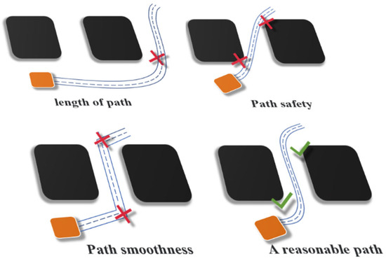
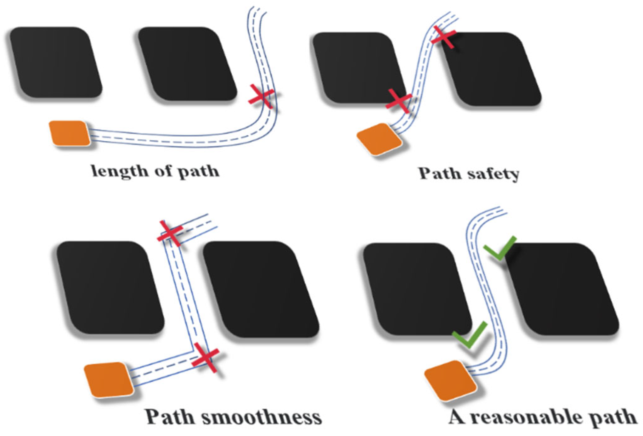
As illustrated in Figure 1, a high-quality planned path must simultaneously satisfy multiple requirements: the path should be as short as possible to reduce task completion time and energy consumption; it must maintain a safe distance from obstacles to avoid collision risks; and it should be smooth, minimizing sharp turns and abrupt changes to reduce mechanical wear on actuators and control difficulty. Based on the above analysis, this paper constructs a mathematical model for the path-planning problem from the following three aspects.
Figure 1.
AGV path-planning model diagram (golden yellow: AGV, black: obstacles).
2.1. Path Length
In path planning for intelligent systems such as autonomous mobile robots and unmanned vehicles, the core objective is not merely to pursue the shortest distance from the start point to the target point, but also to achieve a comprehensive optimum across multiple interdependent dimensions. The shortest path length serves as a direct manifestation of efficiency, closely relating to task completion time and energy consumption. Mathematically, the length of a path segment is typically determined by the Euclidean distance between its two points. Consequently, the total path length is calculated by summing the lengths of all segments that constitute the path. represents a feasible path, where denotes the start point and denotes the target point. The fitness value of the path length can be calculated as follows:
where represents an intermediate point on the path, and denotes the Euclidean distance between and .
2.2. Path Safety
When operating in warehousing environments, AGVs must not only avoid collisions with obstacles but also maintain a certain safety margin to account for uncertainties such as sensor errors and control deviations. Therefore, path safety constitutes a non-negotiable hard constraint in planning. This implies not merely that the path must be geometrically collision-free with respect to known obstacles, but also emphasizes the proactive maintenance of an adequate safety margin. Accordingly, the fitness value of path safety can be calculated as follows:
where denotes the minimum distance from point to the obstacle set , and is a very small positive number used to prevent the denominator from being zero.
To prevent numerical instability when path points approach obstacles, the safety function is normalized and a minimum distance threshold is enforced, which corresponds to the minimum safe clearance for the AGV in the warehouse. This threshold can be adjusted according to vehicle dimensions and operational requirements.
2.3. Path Smoothness
Having ensured the safety of the path, another critical metric is path smoothness. A path that is safe yet filled with sharp turns and acute angles forces the AGV to accelerate, decelerate, and steer frequently, which not only increases energy consumption and mechanical wear on the actuators but may also lead to motion instability, reduced control accuracy, and even interference with the normal operation of onboard equipment (such as camera vibration or abnormal sensor data). Therefore, smoothness is introduced as an optimization objective; minimizing this metric effectively suppresses curvature variations along the path, promoting the generation of continuous, gentle, and easily trackable trajectories, thereby enhancing overall motion quality and system reliability. Its mathematical formulation is expressed as the sum of squared second-order differences of three consecutive points along the path:
where are three consecutive points along the path, and denotes the Euclidean norm.
2.4. Complete Mathematical Model
While ensuring the obtained path is as short as possible, it is also necessary to guarantee that the path points do not lie on obstacles and remain at a safe distance from them, and that the path line avoids collisions with obstacles while maintaining few turns and good smoothness. Based on the above considerations, the mathematical model for the path planning problem is formulated as follows:
where and are customizable weight parameters that can be adjusted according to specific engineering requirements. In this study, the following parameter values are adopted in both the simulations and experiments: ; denotes the shortest path length; represents the set of obstacles in the map; and indicates that the path has no intersection with obstacles, i.e., it is collision-free.
The coefficients , , and were selected based on the relative importance of path length, safety, and smoothness in warehouse operations. A preliminary sensitivity analysis was conducted by varying these coefficients within ±10–20%, and the results show that such variations do not significantly affect the optimized paths, indicating the robustness of the model.
3. Proposal of the Enhanced Harris Hawks Optimization (EHHO) Algorithm
3.1. Targeted Enhancement Strategy
The standard HHO algorithm initializes the first-generation individuals through random initialization and subsequently proceeds to two phases: exploration and exploitation. The transition between these phases is governed by the prey’s escape energy EE, which decreases linearly from 2 to 0 with the number of iterations. When , the algorithm is in the exploration phase, searching for prey across different regions; when |E| < 1, it enters the exploitation phase and performs a dive toward the prey. To address the three core deficiencies of the standard HHO algorithm identified in the introduction, this section introduces three synergistic improvement strategies, corresponding respectively to initial population optimization, balancing the search process, and a mechanism for escaping local optima.
3.1.1. Initialization Strategy Based on Enhanced Sine Chaotic Mapping
Unlike other optimization problems, path planning typically requires generating continuous and smooth paths in complex, obstacle-rich environments while demanding that the algorithm converges rapidly to feasible solutions. Therefore, the initialization strategy necessitates those individuals be distributed as uniformly as possible and cover the entire search space—requirements that random initialization cannot adequately satisfy. A chaotic mapping approach should be adopted to transform random solutions into uniformly distributed ones. This paper introduces an enhanced sine chaotic mapping, which incorporates an adjustable parameter μ, resulting in superior ergodicity and uniformity in the phase space compared to the traditional sine mapping. This mechanism improves algorithm performance in the following three aspects. First, a uniformly distributed initial population effectively avoids the clustering of individuals caused by random initialization, enhances the diversity of initial solutions, and lays a foundation for subsequent global search. Second, in path-planning problems, the continuity of initial path points directly affects the quality of feasible solutions; uniform distribution facilitates the generation of initial paths that do not cross obstacles in complex environments, reduces the proportion of infeasible solutions, and aligns well with the newly proposed mathematical model for warehousing environment path planning, making it easier to discover smoother and safer paths. Third, the ergodic nature of chaotic mapping ensures that the initial population achieves multi-scale coverage of the solution space, enhancing the algorithm’s ability to explore different regions simultaneously during the early stage. This mechanism does not introduce additional parameter tuning burden, preserving the structural simplicity of HHO while providing better initial conditions for balancing exploration and exploitation. The original sine chaotic mapping formula is as follows:
where a is a control parameter, typically set to .
The enhanced sine chaotic mapping formula is as follows:
where represents the chaotic control parameter, which determines the nonlinear strength and the degree of chaos.
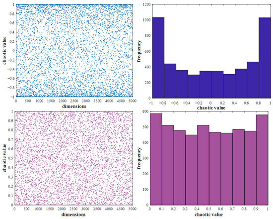
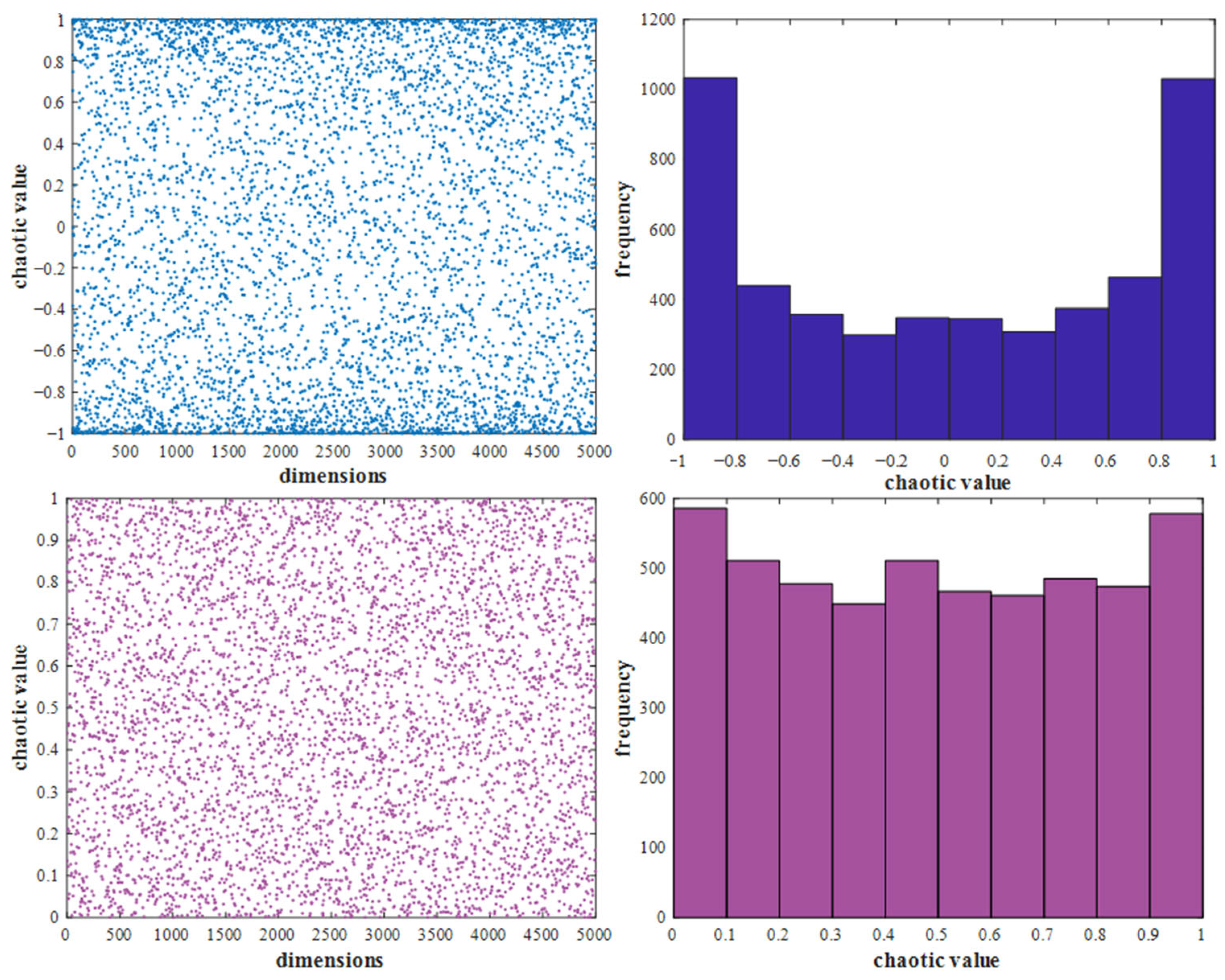
The comparison of particle distribution and particle frequency before and after applying chaotic mapping is shown in Figure 2 (). It can be observed that, after chaotic mapping, the particle distribution becomes highly uniform. Such a strategy typically exhibits more balanced and robust performance in structurally constrained problems such as path planning. While maintaining population quality, it naturally promotes path continuity and smoothness, effectively avoiding obstacle boundaries in complex environments while providing multi-scale search capabilities to accelerate convergence, ultimately generating high-quality initial paths that meet the requirements of practical problems.
Figure 2.
Comparison before and after chaotic mapping: (Top) before improvement; (Bottom) after improvement.
3.1.2. Improved Energy Factor and Escape Energy
In the original algorithm, the transition between exploration and exploitation phases in Harris Hawks is controlled by the prey’s escape energy, which exhibits a linear decreasing trend. This linear decay strategy cannot simultaneously ensure sufficient global exploration in the early stage and rapid convergence in the later stage. As the number of iterations increases to a certain extent, the Harris Hawks are confined to local search and become prone to falling into local optima. Therefore, this paper proposes a nonlinear energy factor to balance the strategy switching between exploration and exploitation, enabling the algorithm to perform broad global search in the early stage and rapidly determine the optimal position during local exploitation in the later stage, thereby improving the convergence speed. The formulas for the original energy factor and escape energy E, as well as the improved energy factor and escape energy , are shown in Equation (7) and Equation (8), respectively:
where denotes the initial energy, which is randomly varied in the range , t is the current iteration number, and is the maximum number of iterations. represents the improved escape energy, and represents the improved energy factor.
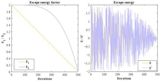
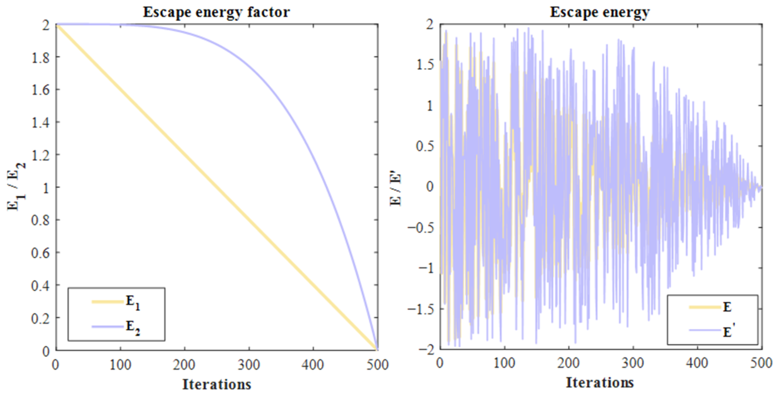
Figure 3 shows the comparison curves of the energy factors ( and ) and escape energies ( and ) before and after improvement when the number of iterations is 500. It can be observed that both the improved and exhibit a slow decline in the early stage, which ensures extensive global search during the initial phase and prevents the algorithm from falling into local optima, while the decline rate accelerates in the later stage, enabling the algorithm to converge rapidly to the global optimal solution and improving the convergence speed.
Figure 3.
The escape energy factor and escape energy before and after the improvement.
The core of this mechanism lies in dynamically adjusting the energy decay rate to achieve the stage-wise control of search behavior, thereby avoiding the issue of premature convergence caused by the linear strategy entering the exploitation phase too quickly in the early stage. Moreover, this improvement does not alter the original framework of HHO but only reconstructs the energy factor, incurring negligible computational overhead, while enhancing the algorithm’s adaptability to multimodal, high-dimensional complex problems.
3.1.3. Pinhole Imaging Opposition-Based Learning Strategy
To more effectively prevent the algorithm from becoming trapped in local optima, this paper introduces an opposition-based learning strategy inspired by the pinhole imaging principle. The core idea of this strategy is to generate a corresponding opposition solution for the current global optimal solution in each iteration, and then select the better one to enter the next generation by comparing their fitness values. Drawing on the pinhole imaging mechanism in optics, this method constructs a corresponding opposition mapping for each dimension of the current solution. Unlike traditional opposition-based learning, the pinhole imaging strategy introduces an adjustable scaling factor n to map the current global optimal solution into a dynamic opposition solution. This scaling factor n increases linearly with the number of iterations, enabling an adaptive adjustment of the range within which the opposition solution is generated. In the early iteration stage, n is small, resulting in a larger span for the opposition solution, which helps to escape the current local extremum region and expands the search range. In the later stage, n approaches 1, and the opposition solution gradually converges toward the vicinity of the current optimal solution, enhancing local refined search capability. Compared with traditional opposition-based learning, this mechanism does not rely on fixed boundary mapping but generates opposition points dimension by dimension, thereby avoiding inter-dimensional interference and improving the effectiveness of the opposition solution. Consequently, it helps the algorithm to break free from the constraints of the current optimal region and progressively approach the global optimal region. This strategy not only contributes to increasing population diversity and extending the search range of the algorithm, but also reduces inter-dimensional interference through dimension-wise mapping, effectively enhancing the algorithm’s global exploration capability and its ability to escape local optima. The specific formula for this strategy is as follows:
where is the inversely generated image, is the position of the prey, and and denote the upper and lower bounds of the population, respectively.
It can be observed from the formula that the scaling factor n increases linearly from 0 to 1 over the course of iterations. This means that the opposition solution spans a wider search range during the early stage, enabling better exploration within the search domain, while the span gradually narrows in the later stage, causing the opposition solution to be generated near the current optimal solution in each iteration. This effectively aligns with the search requirements at different stages of the iterative process.
3.2. The Enhanced Harris Hawks Optimization (EHHO) Algorithmic Framework
3.2.1. New Initialization Strategy and Calculation of the New Prey Escape Energy
First, high-quality initialization individuals are generated using the introduced enhanced sine chaotic mapping. Subsequently, like in the original HHO, the algorithm proceeds into exploration and exploitation phases based on the dynamic nature of the scenario and the prey’s escape pattern. However, the transition between these two phases is governed by the new prey escape energy: obtained from Equation (8) is used to derive through and , and the choice of strategy is determined by . The new prey escape energy exhibits a nonlinear decreasing trend. When , the algorithm is in the exploration phase, searching for prey across different regions; when , it enters the exploitation phase and performs a dive toward the prey.
3.2.2. Exploration Phase
When , the Harris Hawks randomly search for prey across the global exploration range, which is specifically manifested in two distinct approaches to locating the prey:
where is the maximum population size, is the current iteration position, is the next iteration position, is the position of the i-th individual in the population, is the position of the prey, rand are random numbers in , is the position of a randomly selected individual from the current population, and and are the upper and lower bounds of the population, respectively. denotes the average position of the current population.
3.2.3. Exploitation Phase
When , four strategies are employed to simulate the attacking behavior of Harris Hawks during the predation stage. Among these, the random number is used to simulate the randomness of the prey’s escape behavior. When , this indicates that the prey fails to escape; when , this indicates a higher probability of successful escape. The update strategy is determined jointly by and .
Soft Encircling Strategy: When and (the prey still has some energy and attempts to escape with random jumps),
where represents the difference between the current optimal solution and the individual solution, denotes the random jump intensity of the prey throughout the escape process, and is a random number in .
Hard Encircling Strategy: When and (the prey is extremely exhausted with very low escape energy),
Progressive Soft Encircling Strategy: When and (a more intensive soft encircling strategy),
where denotes the fitness function, is a random vector (where is the dimensionality of the problem), and represents the flight function, which is calculated as follows:
where is a default parameter, typically set to 1.5, and are random variables in , and denotes the standard gamma function.
Progressive Hard Encircling Strategy: When and (the prey’s energy is exhausted, and a surrounding circle is established to ensure successful capture),
3.2.4. Based on the Pinhole Imaging Opposition-Based Learning Strategy, Generate the Reverse Solution
After completing the position update for all individuals in the current iteration, the algorithm introduces the pinhole imaging opposition-based learning strategy to further enhance population diversity and assist in escaping local optima. As an independent step within the EHHO algorithm framework, this strategy is executed at the end of each iteration. It generates a corresponding opposition solution based on the current global optimal solution using the pinhole imaging principle and retains the better individual for the next generation through fitness comparison.
The specific implementation of this strategy follows Formula (9) provided in Section 3.1.3, where the scaling factor n increases linearly with the number of iterations. Consequently, opposition solutions with a larger span are generated in the early stage to expand the search range, while opposition solutions converging near the optimal solution are generated in the later stage to enhance local refined search capability. This step does not alter the asymptotic time complexity of the algorithm but effectively improves its ability to escape local optima, forming a complete closed loop of improvements together with the chaotic initialization and the nonlinear energy factor.
3.3. Enhanced Harris Hawks Optimization (EHHO) Algorithm Flow and Analysis
3.3.1. Analysis of Algorithm Time Complexity
The fundamental operations of the original Harris Hawks Optimization algorithm determine that its time complexity primarily depends on the maximum number of iterations , population size , and problem dimensionality . Its core procedures, including population initialization and position updates during the exploration and exploitation phases , collectively constitute its overall time complexity of . In the improved EHHO algorithm, the enhanced sine chaotic mapping performs chaotic mapping on the initial individuals, which shares the same order as the original initialization, both being , and does not change the order of magnitude. The nonlinear energy factor computes a new nonlinear factor in each iteration, incurring a constant overhead of , which is negligible. The pinhole imaging opposition-based learning strategy generates an opposition solution for the global optimal solution and performs one evaluation per iteration, adding a fixed overhead of per iteration. Consequently, the total time complexity of the EHHO algorithm is . The complexity of EHHO is primarily dominated by , while the additional overhead is negligible, and this expression can be simplified to . Therefore, the asymptotic time complexity of the EHHO algorithm remains consistent with that of the original HHO algorithm, and the introduced improvement strategies do not cause an increase in the order of magnitude of computational burden.
3.3.2. Flowchart and Pseudocode of the EHHO Algorithm
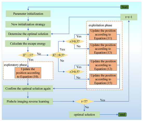
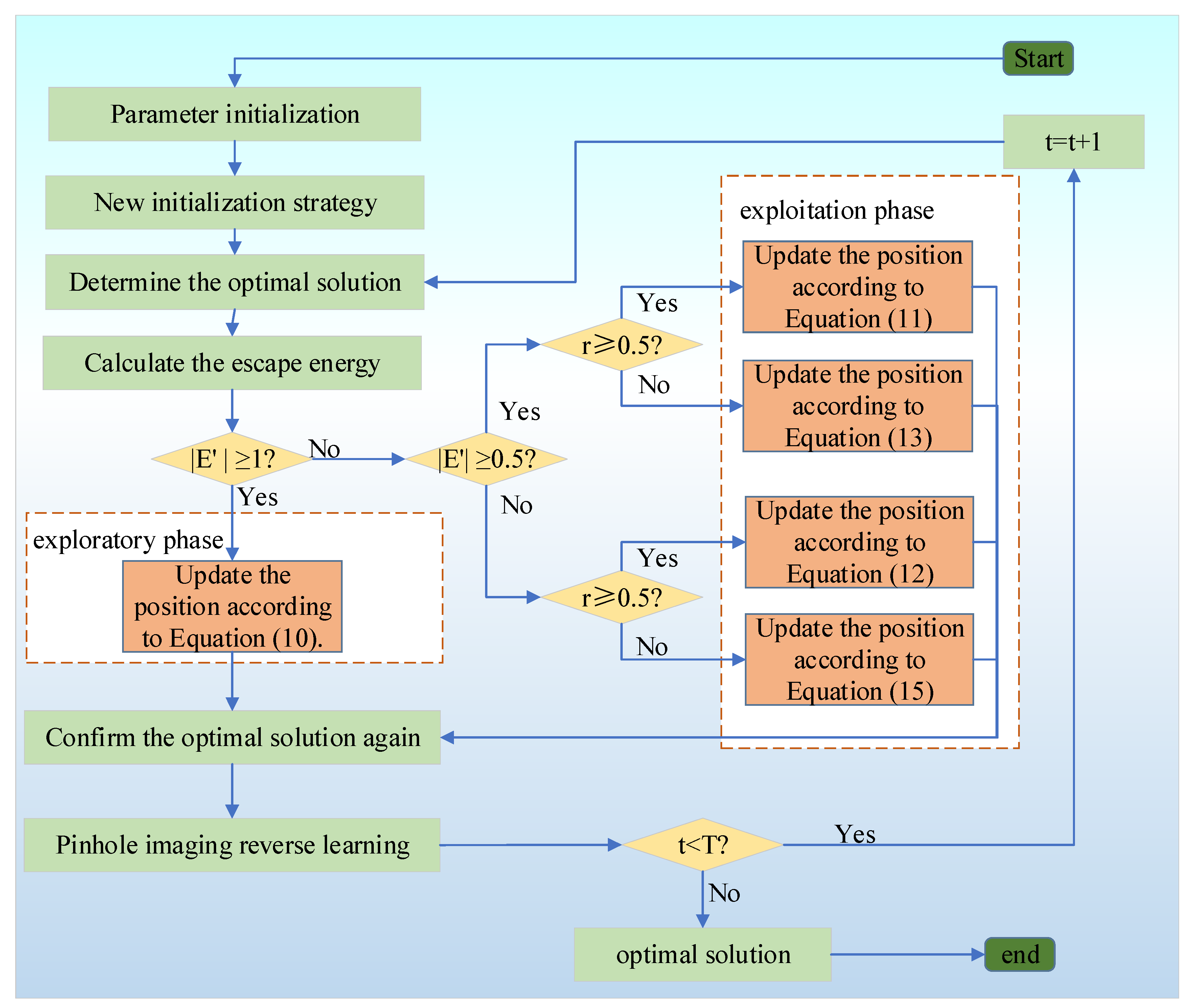
Based on the above, this paper improves the HHO algorithm by introducing three strategies and proposes the EHHO algorithm. The algorithm procedure is as follows, and its flowchart is shown in Figure 4; the pseudocode of EHHO is provided in Algorithm 1, based on which the algorithm procedure is visualized.
| Algorithm 1. Pseudocode of EHHO |
| Input: population size N, iterations T, and objective function |
| Output: The location of rabbit and its fitness value |
| 1. Initialize the random population |
| 2. Apply the enhanced sine chaotic mapping to each eagle |
| 3. while t ≤ T do |
| 4. Calculate the fitness function for each hawk |
| 5. Update the position of the rabbit based on the fitness |
| 6. For each hawk do |
| 7. Update escape energy E according to Formula (8) |
| 8. If then |
| 9. Update the position according to Formula (10) |
| 10. else |
| 11. if and then |
| 12. Update the position according to Formula (11) |
| 13. else if and then |
| 14. Update the position according to Formula (13) |
| 15. else if and then |
| 16. Update the position according to Formula (12) |
| 17. else |
| 18. Update the position according to Formula (15) |
| 19. end if |
| 20. end if |
| 21. end for |
| 22. Calculate the fitness function for each hawk |
| 23. generate the reverse solution for the current optimal solution (Formula (9)) |
| 24. select the best one |
| 25. Set t = t + 1 |
| 26. end while |
| 27. Returned |
Figure 4.
Flowchart of the EHHO algorithm.
3.3.3. Convergence Analysis of the EHHO Algorithm
Through the convergence analysis of the swarm intelligence algorithm, it is proven that the algorithm can stably converge to the optimal solution in the problem space under certain conditions. This mainly involves two aspects: theoretical proof and benchmark function testing. The convergence test results are presented in Section 4, and the theoretical proof is provided in Appendix A. Through Lyapunov Stability Derivation, the EHHO algorithm demonstrates expected Lyapunov stability. For any initial population, the algorithm’s trajectories remain bounded and iteratively move closer to the global optimum, showing both convergence stability and robustness to initial conditions. The combination of chaotic initialization, nonlinear convergence factor, and opposition-based learning provides a balance between exploration and exploitation while maintaining stability.
4. Simulation and Experimental Results Analysis
4.1. Classical Functions
All simulation experiments were conducted in MATLAB R2023a on a Windows 11 platform equipped with an Intel(R) Core (TM) i5-9300H processor and 8 GB RAM. To assess the optimization capability of the proposed EHHO algorithm under different search landscapes, twelve representative functions were selected from the CEC benchmark suite. These functions cover several optimization characteristics, including unimodal, multimodal, and composite scenarios. Among them, F1–F5 correspond to unimodal functions with a dimensionality of 30, mainly used to evaluate convergence capability and local exploitation performance. F6–F9 are multimodal functions designed to test the global exploration ability of the algorithms in complex search spaces, while F10–F12 are composite functions that combine multiple landscape features to further examine optimization robustness and overall search performance. The mathematical expressions of the benchmark functions are summarized in Table 1.
Table 1.
Benchmark function.
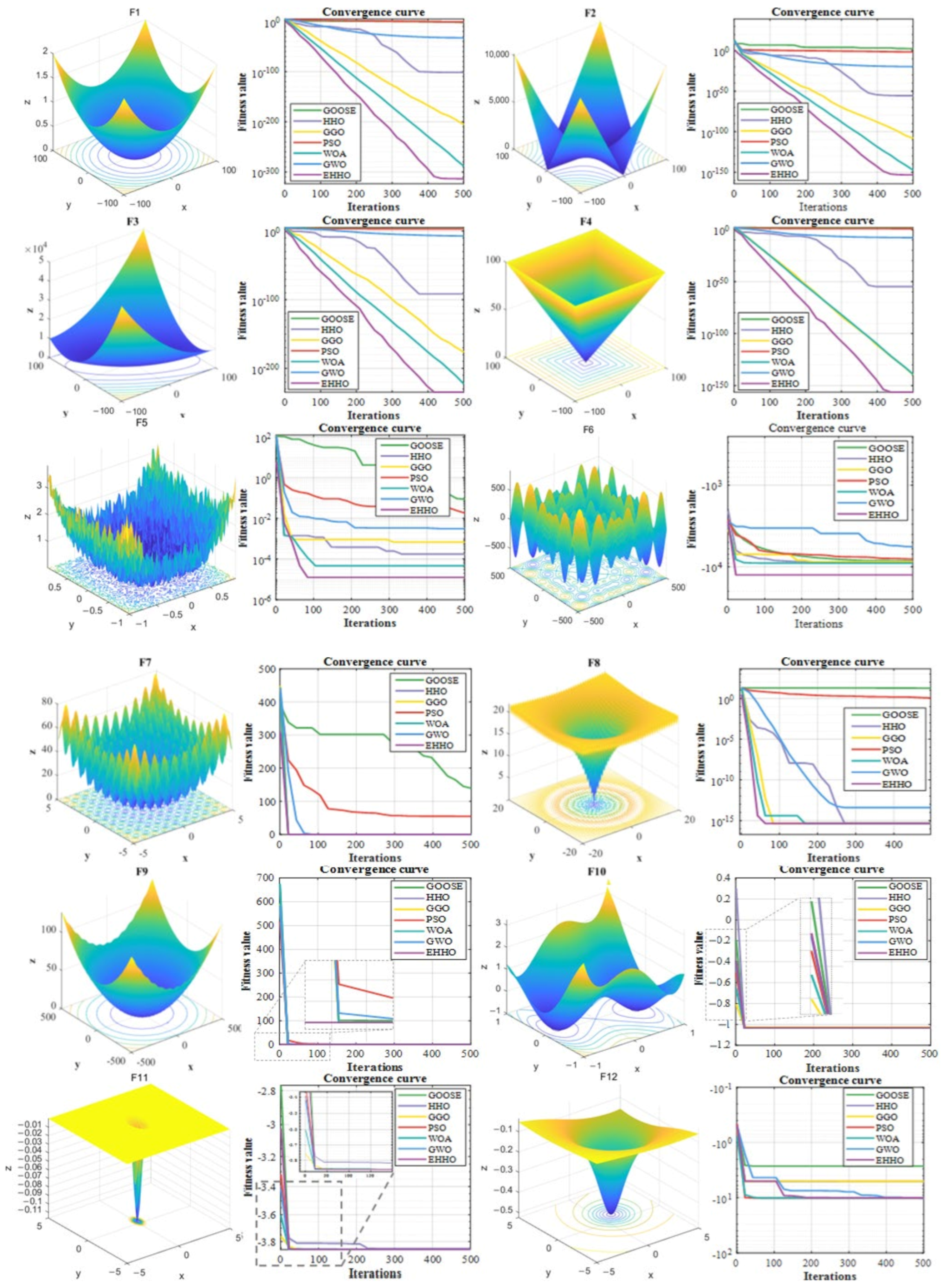
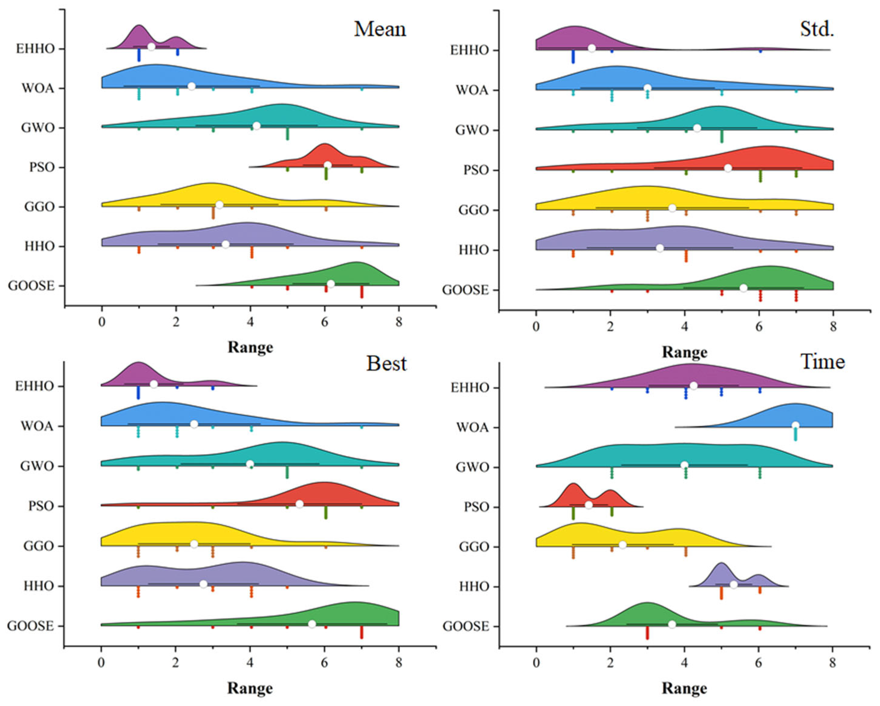
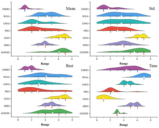
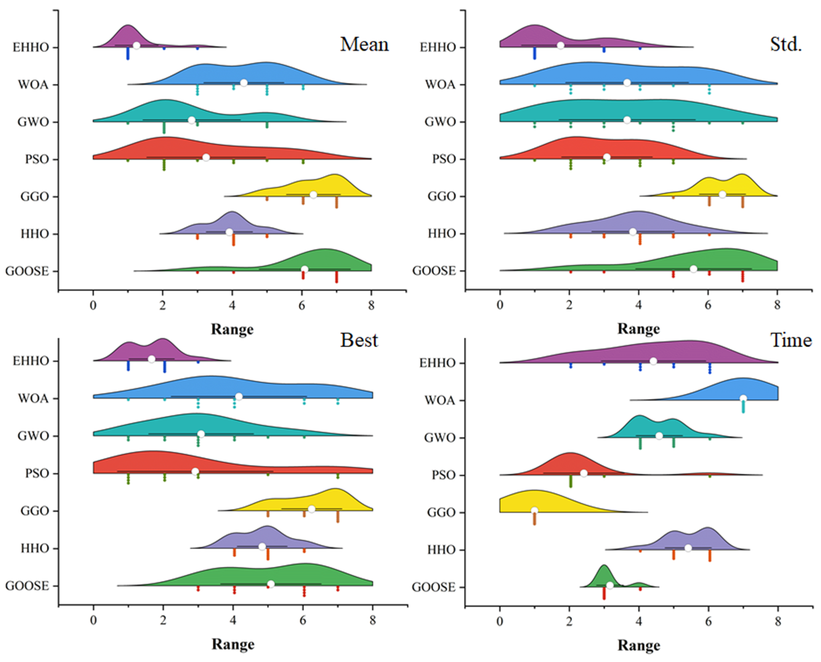
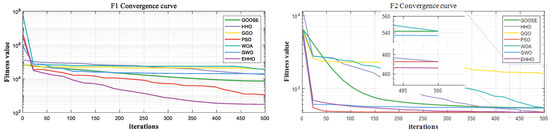
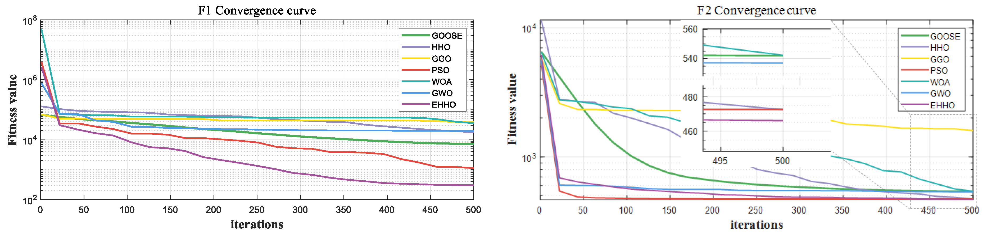
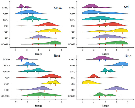
To eliminate the influence of randomness on the test results, these benchmark functions were used to test and compare seven algorithms: the EHHO algorithm, the HHO algorithm, the PSO algorithm, the GGO (Greylag Goose Optimization) algorithm, the GWO (Grey Wolf Optimizer) algorithm, the WOA (Whale Optimization Algorithm), and the GOOSE (Goose Optimization Algorithm). Each algorithm was run independently 30 times on each test function, and the mean, standard deviation, optimal value, and runtime were adopted as performance evaluation metrics. A smaller mean indicates a higher convergence accuracy and stronger optimization capability of the algorithm; a smaller standard deviation indicates lower fluctuation and higher stability. The comparison algorithms were tested against the 12 classical functions listed in Table 1, with the detailed test results presented in Table 2. The three-dimensional function images and the fitness value convergence curves are shown in Figure 5. The ranking of performance metrics in the specific simulation experiments is shown in Figure 6.
Table 2.
Results of classic function tests (bolded ones are ranked first).
Figure 5.
Representative benchmark function landscapes and the corresponding convergence curves of different algorithms (The change from yellow to blue indicates proximity to the optimal solution).
Figure 6.
Classical function test ranking (The upper ‘cloud’ represents the kernel density estimation, and the lower ‘rain’ represents the distribution of individual data points).
Overall, EHHO achieves superior performance in terms of mean value, standard deviation, and best value across most benchmark functions. For unimodal and multimodal functions (e.g., F1–F3, F6–F9), its solution accuracy outperforms that of the comparison algorithms, validating the effectiveness of the nonlinear escape energy factor in balancing global exploration and local exploitation. Its excellent stability benefits from the synergistic effect of hybrid initialization and the opposition-based learning strategy, while its strong global optimization capability reflects the advantage of the pinhole imaging strategy in escaping local optima. In terms of runtime, EHHO achieves shorter computation times than HHO on five functions, including F1, F4, F5, F7, and F8; notably, on F4, its runtime is only 65.1% that of HHO. For most other functions, EHHO incurs a slightly higher runtime than HHO, yet on certain functions it requires less time due to faster convergence. This is attributable to the pinhole imaging opposition-based learning strategy, which introduces additional opposition solution generation and evaluation operations in each iteration, adding a fixed computational overhead. Nevertheless, this marginal increase in runtime is accompanied by a substantial improvement in convergence accuracy and stability (e.g., accuracy improvements of several orders of magnitude on functions F1–F3). The overall performance gain achieved justifies the associated time cost.
4.2. CEC2022 Test Function
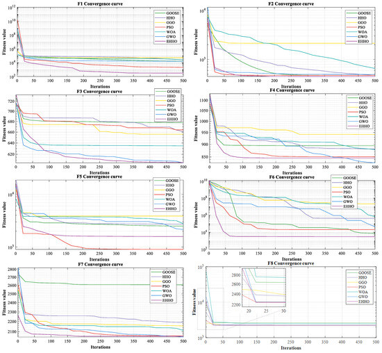
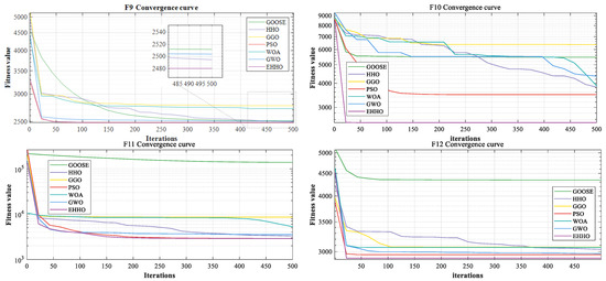
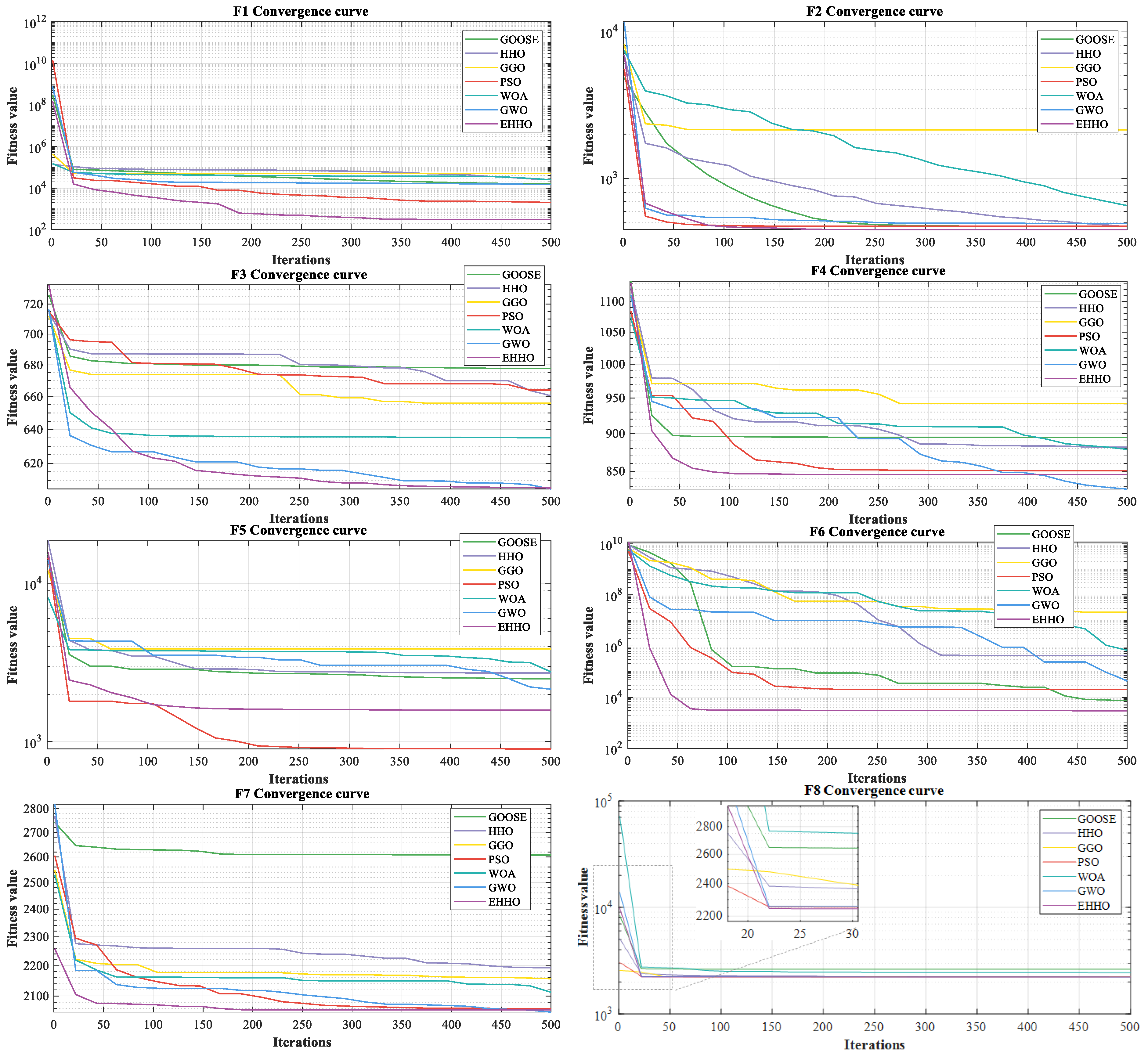
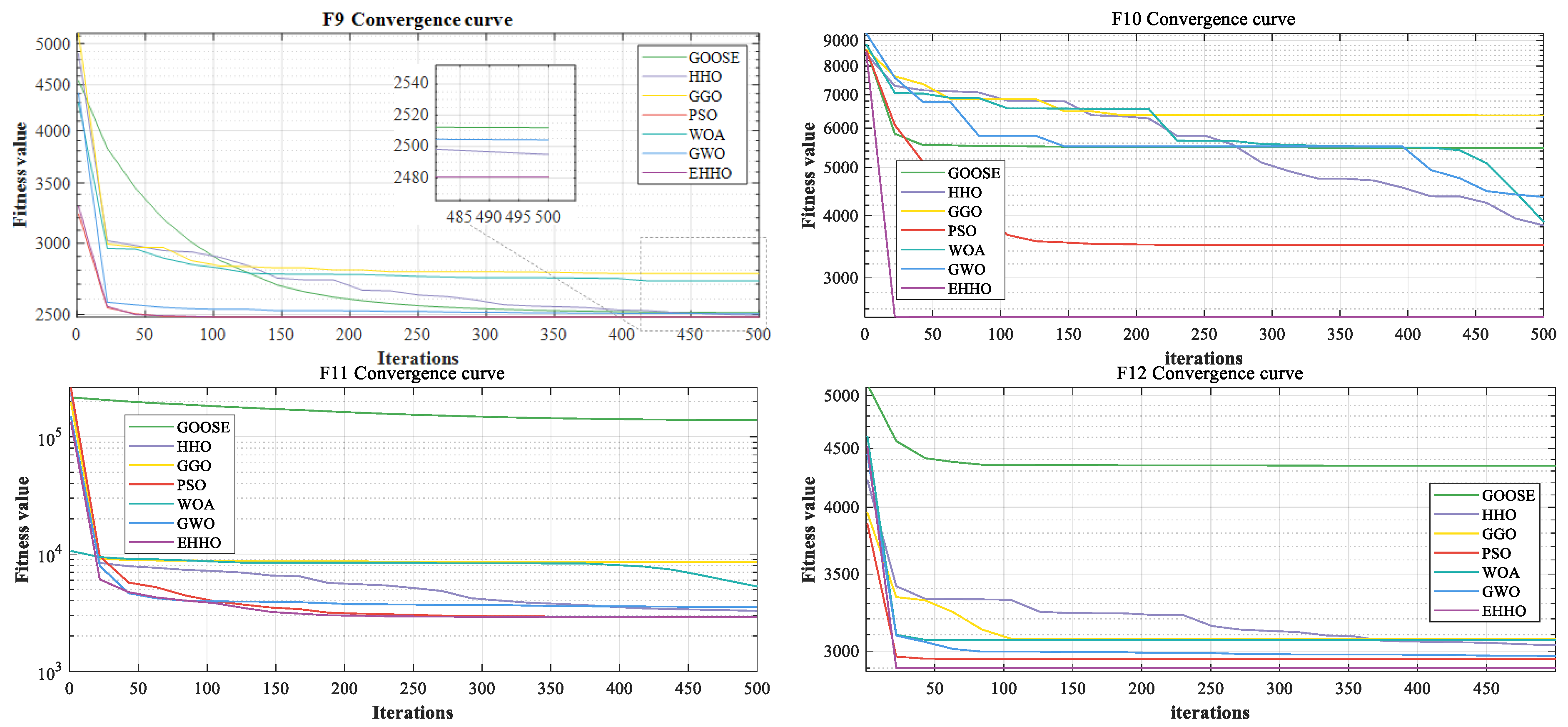
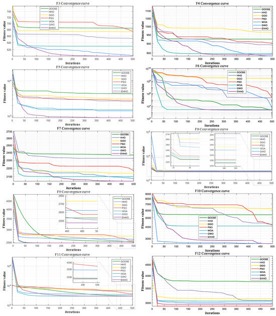
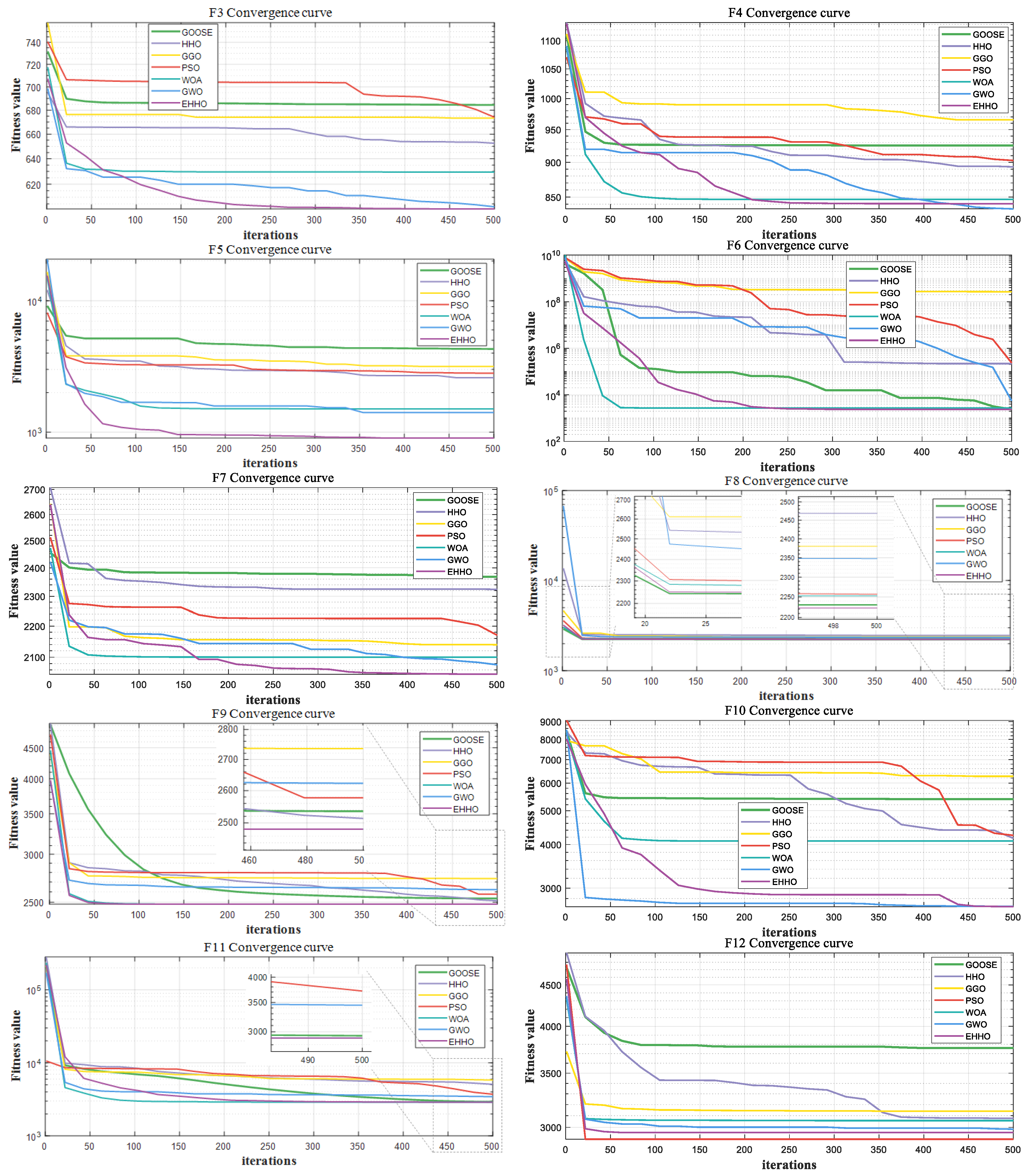
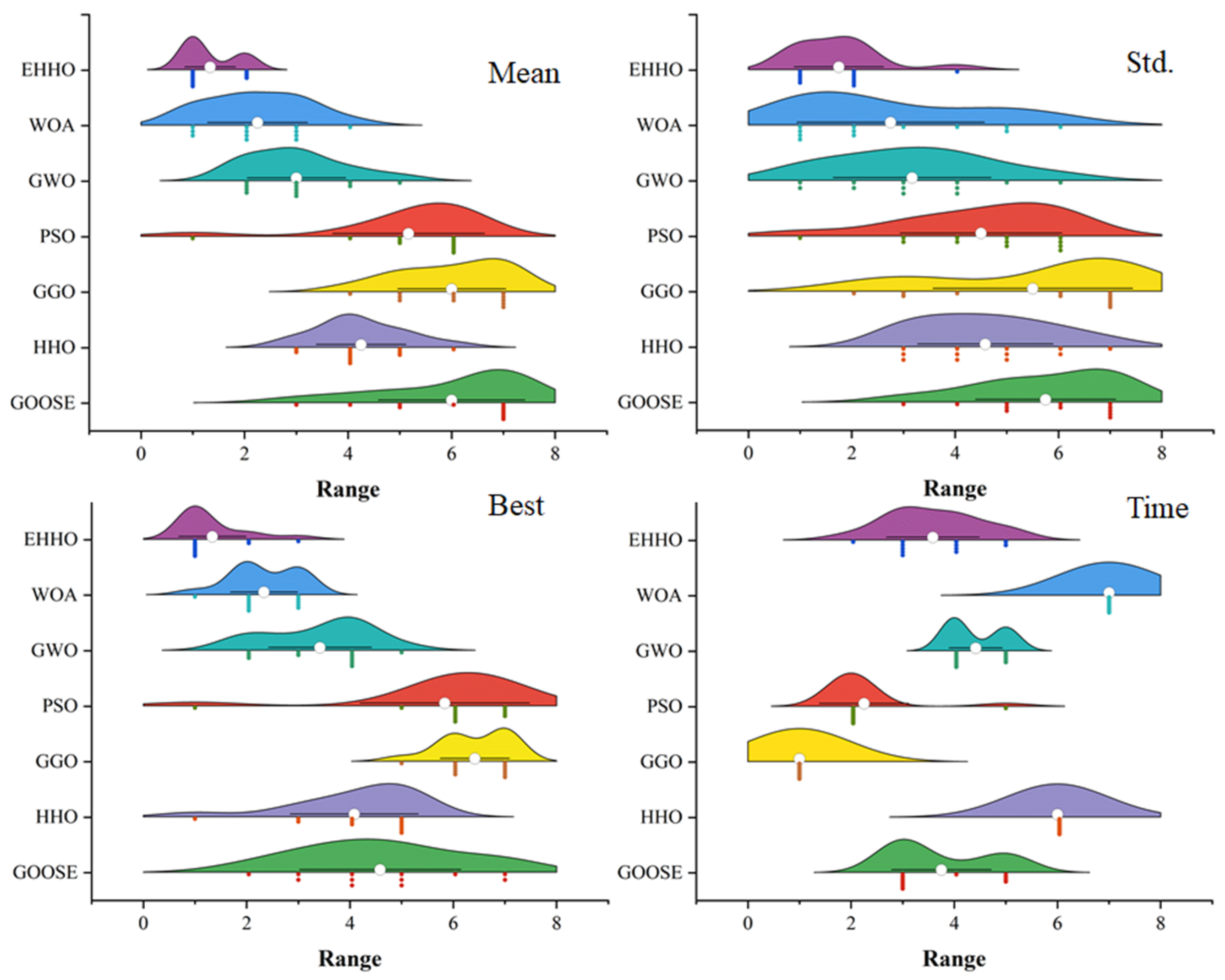
To further validate the optimization performance and robustness of the proposed algorithm on complex benchmark problems, the publicly available CEC2022 benchmark test suite was employed for comparative optimization analysis among seven algorithms under 10-dimensional and 20-dimensional settings. The benchmark suite contains a variety of test functions with different optimization characteristics, and Table 3 summarizes the relevant information of functions F1–F12, including their categories and dimensional settings. The detailed experimental results are reported in Table 4 and Table 5, while the convergence curves and ranking comparisons of the algorithms are illustrated in Figure 7, Figure 8, Figure 9 and Figure 10.
Table 3.
CEC2022 test function details.
Table 4.
CEC 2022 (10-D) function test results (bolded indicates first place).
Table 5.
CEC 2022 (20-D) function test results (bolded indicates first place).
Figure 7.
The convergence curves of fitness values (10-D).
Figure 8.
Test result (CEC 2022 10-D) ranking (The upper ‘cloud’ represents the kernel density estimation, and the lower ‘rain’ represents the distribution of individual data points).
Figure 9.
The convergence curves of fitness values.
Figure 10.
Test result (CEC 2022 20-D) ranking (The upper ‘cloud’ represents the kernel density estimation, and the lower ‘rain’ represents the distribution of individual data points).
Based on the overall experimental results, the improved Harris Hawks Optimization (EHHO) algorithm demonstrates exceptional comprehensive performance. In the 10-dimensional tests, EHHO ranks first in the mean value for 8 out of 12 functions (F1–F3, F5–F9), confirming that the nonlinear escape energy factor enhances convergence accuracy by balancing global exploration and local exploitation. In the 20-dimensional tests, the advantages of EHHO become even more pronounced, ranking first in the mean value for 9 out of 12 functions (F1–F7, F9). In terms of stability, EHHO ranks first in standard deviation for 11 functions (F1–F11) in the 10-dimensional tests and for 8 functions (F1–F6, F8) in the 20-dimensional tests, reflecting the excellent stability ensured by the improved initialization strategy and the pinhole imaging opposition-based learning strategy. Regarding optimization capability, EHHO ranks first in the best value for nine functions (F1–F7, F9–F10) in the 10-dimensional tests and for nine functions (F1–F8, F10) in the 20-dimensional tests, highlighting the unique advantage of the dynamic opposition-based learning mechanism in escaping local optima.
A detailed analysis of time cost reveals a similar trend in computational time comparison between EHHO and HHO. In the 10-dimensional tests, EHHO ranks second in F4 and third in F3 and F5; in the 20-dimensional tests, EHHO ranks third in F3 and F4, and ranks fourth in most other functions. On functions such as F2, F6, and F10, the runtime of EHHO is lower than that of HHO; notably, on the 10-dimensional F2 function, the runtime of EHHO is only 55.6% that of HHO, demonstrating a certain efficiency advantage. For most other functions, EHHO incurs additional computational burden due to the opposition-based learning mechanism, with runtime generally slightly higher than that of HHO and several other algorithms, and, compared with the fastest GGO, considering both 10-D and 20-D functions, EHHO’s average runtime is moderately higher than that of GGO, with an increase of approximately 0.07 s in 10-D and 0.13 s in 20-D. However, in contrast, EHHO consistently obtains better-quality solutions, with average best values lower than those of GGO by approximately 2.03 × 10⁴ across all functions. This indicates a balanced trade-off between computational cost and solution quality: the modest increase in runtime due to additional strategies, such as opposition-based learning and enhanced initialization, is accompanied by notable gains in convergence accuracy and robustness. Therefore, EHHO offers a practical approach for optimization tasks where solution quality and reliability are prioritized alongside reasonable computational efficiency.
4.3. The Application of EHHO Algorithm in Path Planning
4.3.1. Grid Map
The grid method is a spatial partitioning and search strategy commonly used in computer science and engineering, particularly in fields such as path planning and robot navigation. This approach divides continuous space into discrete units or “grids,” each representing a specific region within the space. By doing so, the grid method simplifies the complexity of the environment, enabling path-planning algorithms to operate in a more structured setting. The core idea of the grid method is to treat the entire surrounding environment as a two-dimensional plane and further partition it into multiple equally sized small units, referred to as “grids.” It is simple and effective, effectively reducing the complexity of environmental modeling. Therefore, this paper adopts the grid method to construct the working environment model for mobile robots. In the grid environment, 0 and 1 are used to indicate whether a grid represents an obstacle or a free space.
4.3.2. Path-Planning Simulation Experiment and Results
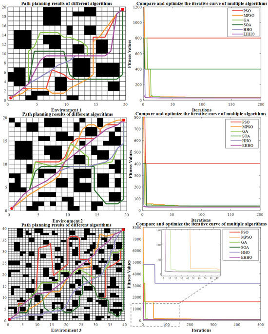
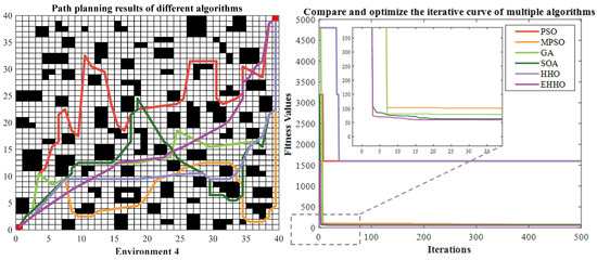
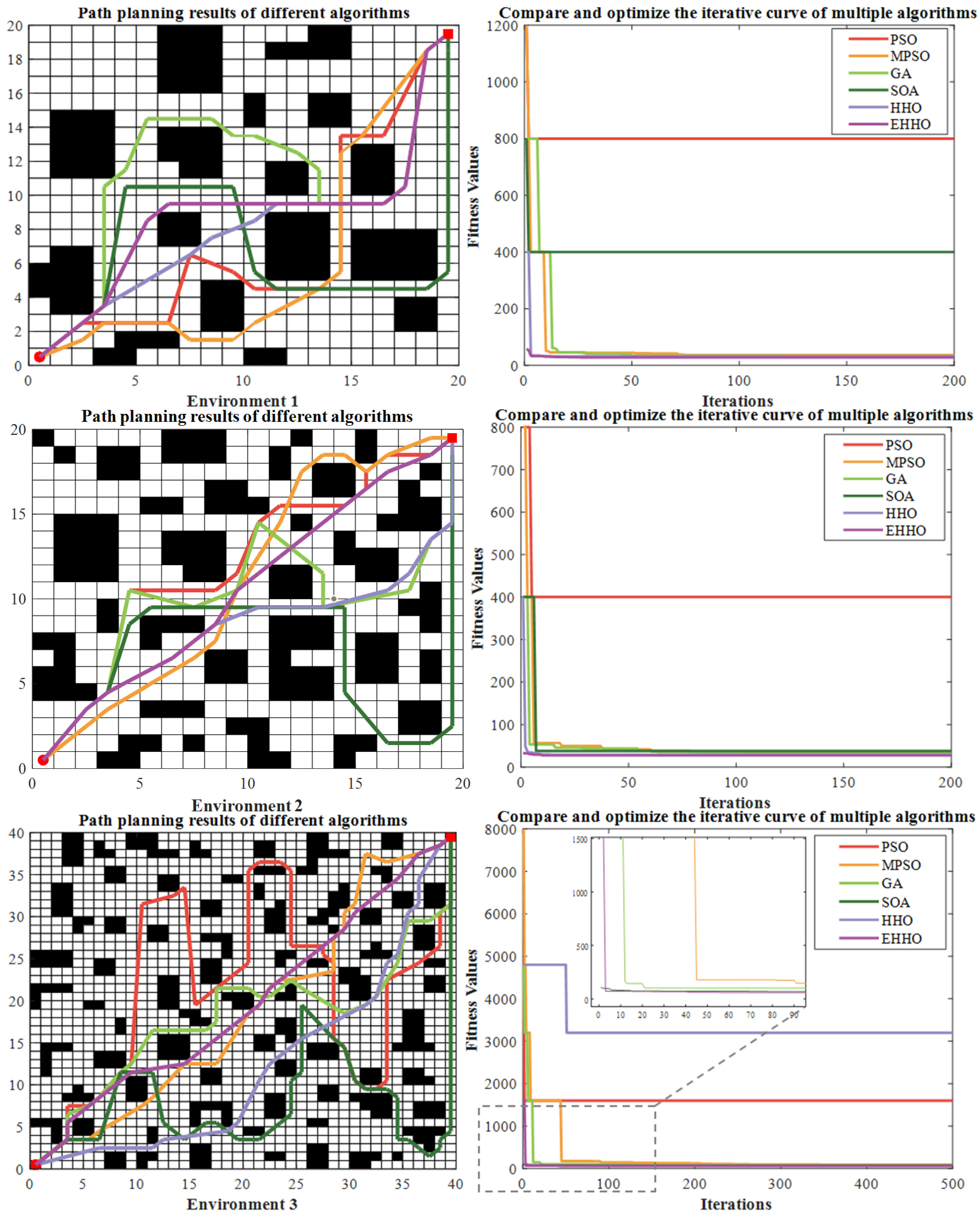
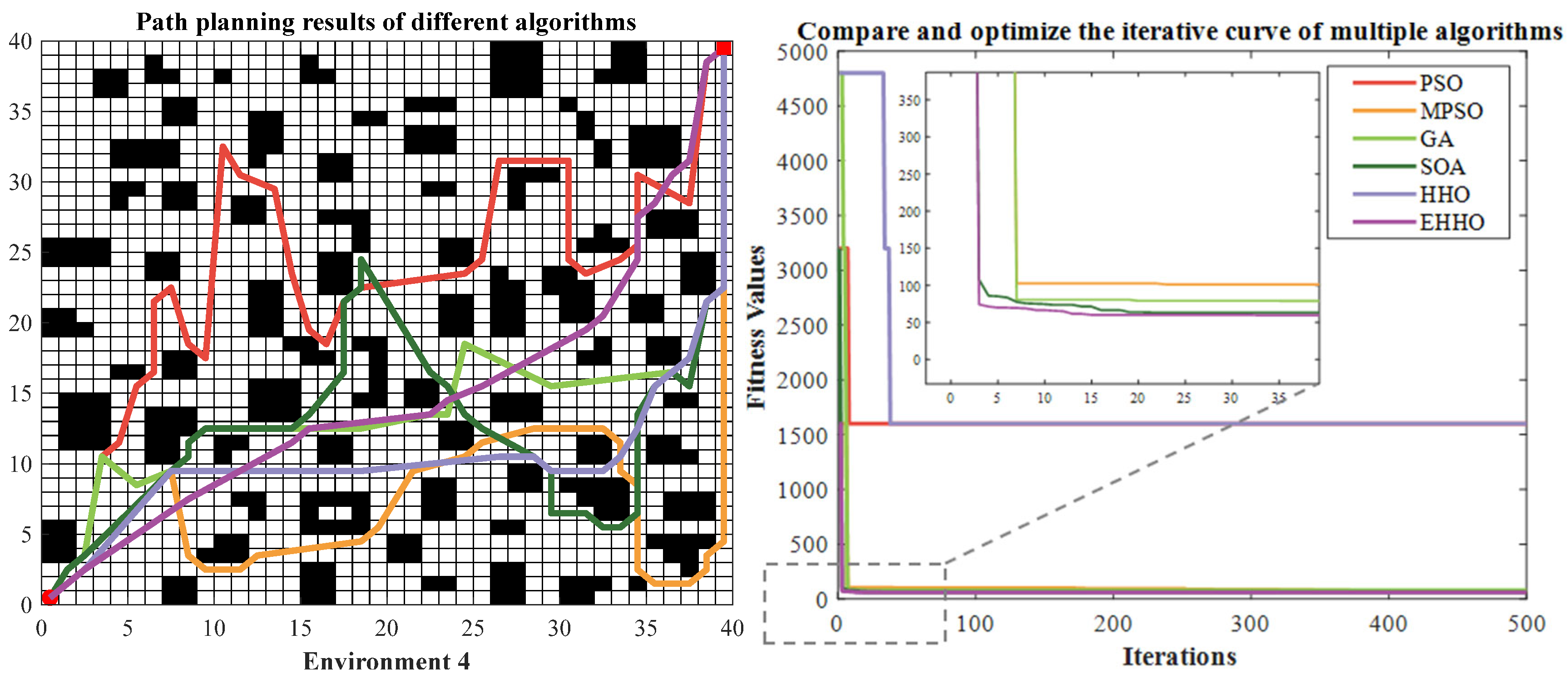
To evaluate the performance of the path-planning algorithms in different scenarios, the simulation environments are categorized into simple and complex types based on obstacle proportion, with two grid sizes of 20 × 20 and 40 × 40, respectively. Map 1 contains a relatively small number of obstacles, which are regularly shaped and sparsely distributed, leaving a sufficiently wide feasible passage between the start and target points. Map 2 features an increased number of obstacles with irregular shapes and dense distribution, presenting multiple narrow passages and greater planning difficulty. Map 3 is larger in size but maintains a similar obstacle proportion to Map 1, primarily serving to test the scalability of the algorithms in larger spaces. Map 4 represents a challenging environment characterized by both large scale and high complexity, with intricate obstacle structures designed to comprehensively evaluate the global planning and local obstacle avoidance capabilities of the algorithms. To validate the effectiveness of the proposed EHHO algorithm in path planning, six algorithms—PSO, MPSO (Multi-Strategy PSO) [19], GA, SOA (Seagull Optimization Algorithm), and the standard HHO algorithm—are selected for comparison, and simulation experiments are conducted on unified grid maps. The population size and number of iterations for all algorithms are set to 50 and 300, respectively. Ten simulation experiments are performed for each of the six algorithms on the two 20 × 20 maps and the two 40 × 40 maps, and the mean fitness value (mean), standard deviation (std.), best value (best), and algorithm simulation time (time) are adopted as evaluation metrics. The specific simulation results are presented in Table 6, while the fitness value convergence curves and path comparison graphs are shown in Figure 11.
Table 6.
Comparison of optimization results for different intelligent algorithms (bolded indicates first place).
Figure 11.
Convergence curves and path-planning results for different algorithms in grid-map environments (The left and right diagrams share the legend in the right diagram).
This section comprehensively evaluates the performance of the Enhanced Harris Hawks Optimization (EHHO) algorithm through systematic simulation experiments, ranging from benchmark function tests to practical path-planning applications. In the path-planning experiments, EHHO demonstrates advantages across grid maps of varying sizes and complexities. Specifically, on the 20 × 20 map (Map 1), the average path length of EHHO is reduced by 10.29% compared to the original HHO algorithm; on the 20 × 20 map (Map 2), the reduction reaches 29.31%, highlighting the effectiveness of the improved strategies in environments ranging from simple to moderate complexity. On the more complex 40 × 40 maps, EHHO maintains stable performance improvements, with average path length reductions of 7.11% and 5.20% on Map 3 and Map 4, respectively.
In terms of algorithmic stability, EHHO also performs well. Across all test maps, the standard deviation of path length obtained by EHHO is lower than that of HHO and other compared algorithms. For instance, on the 20 × 20 map (Map 2), the standard deviation of EHHO is lower than HHO’s value of 1.5134. Moreover, in terms of the “best value” metric across all maps, EHHO consistently identifies shorter paths than HHO, indicating smaller fluctuations across multiple runs, better robustness, and less sensitivity to the initial random population. Overall, compared to the original HHO, EHHO achieves a 12.98% reduction in average path length while improving stability and reliability.
Regarding computational efficiency in the path-planning simulations, EHHO generally achieves comparable or faster runtimes than the original HHO algorithm, except for the larger 40 × 40 maps, where runtimes are similar. Compared with faster algorithms such as PSO, EHHO’s average runtime is slightly higher—about 0.873 s on average across the four test maps—but it consistently produces shorter paths, with an average reduction of approximately 53.81 m in path length. These results indicate that EHHO achieves a favorable balance between computational efficiency and path quality, providing smoother, safer, and more reliable paths for practical AGV deployment. Considering that warehouse AGV path planning generally emphasizes path safety and stability in addition to computation time, the proposed remains acceptable for practical applications.
These results confirm that the proposed enhanced sine chaotic mapping, nonlinear energy factor, and pinhole imaging opposition-based learning strategy effectively improve algorithm performance in path-planning problems, particularly in solution quality, convergence accuracy, and robustness.
4.4. Real Warehouse Environment Experiment
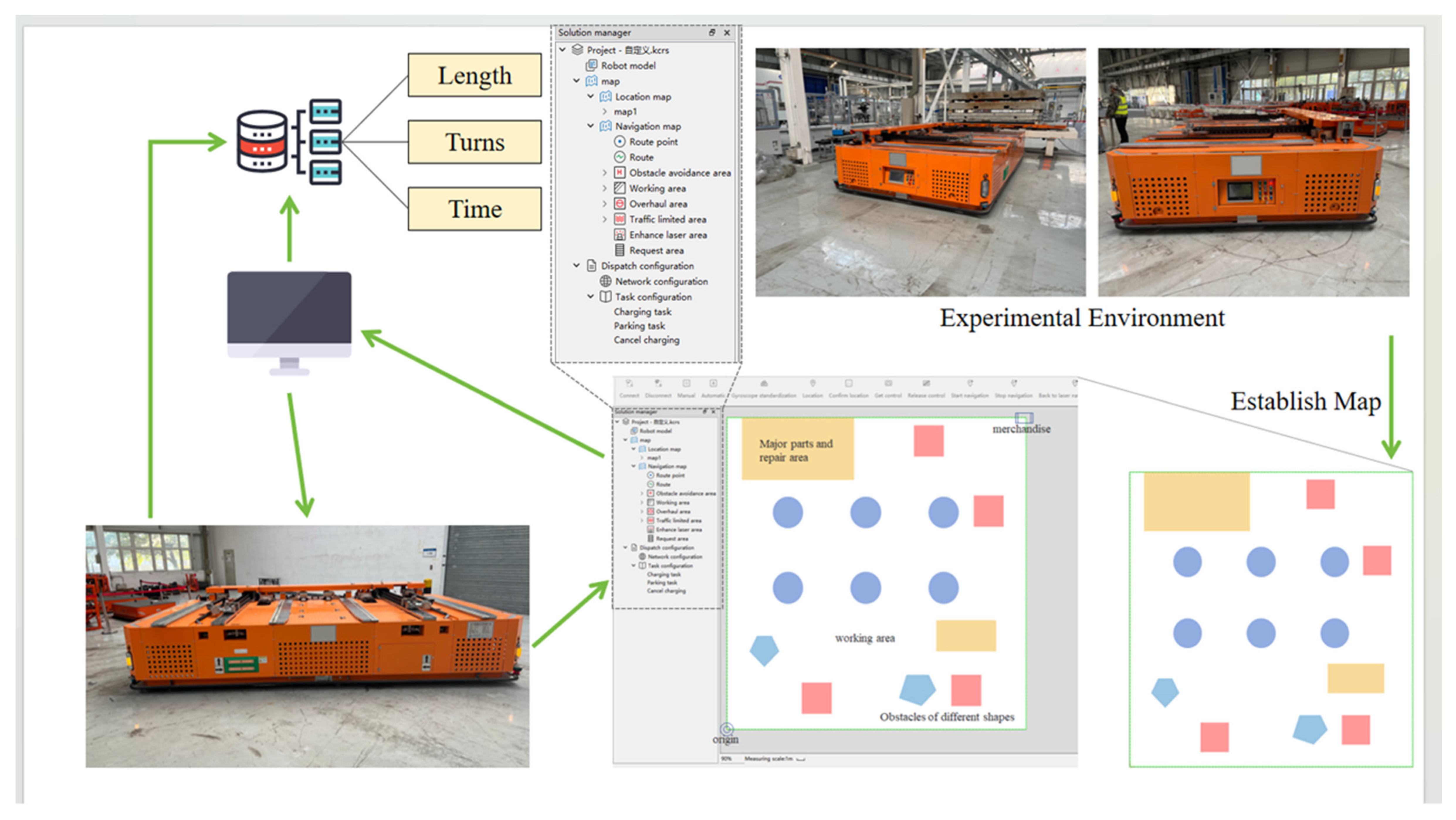
To validate the transferability of the EHHO algorithm in real-world warehousing environments, this study selects a simulated warehouse with an area of approximately 458 square meters as the test scenario. In this scenario, typical obstacles such as shelves and workstations are reasonably arranged to replicate the complex layout of an actual warehousing environment. The corresponding warehouse environment is illustrated in Figure 12. A 20-ton differential-drive AGV is employed as the experimental platform, The prototype has a size of 5 × 2.7 m and uses a multi-sensor fusion system that integrates light detection and ranging (LiDAR), inertial measurement units (IMUS), infrared laser sensors, and Beidou satellite navigation modules, with a linear velocity set to 0.6 m/s and an angular velocity set to 0.3 m/s to simulate motion characteristics under actual operating conditions.
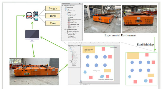
Figure 12.
Flow chart of the experiment.
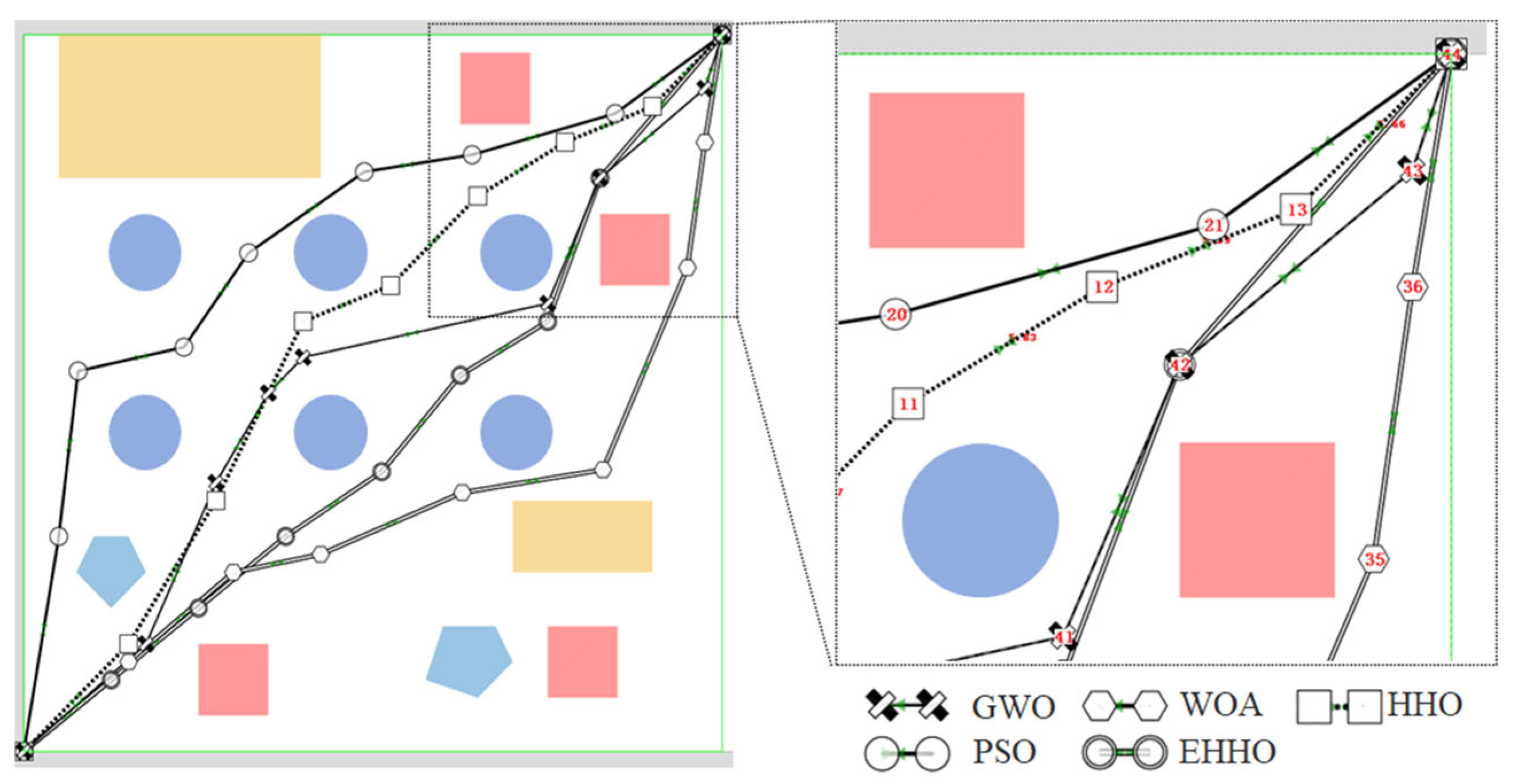
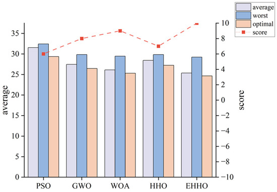
Five path-planning algorithms—namely, EHHO, HHO, PSO, GWO, and WOA—were implemented in the MATLAB environment for comparison. First, a map corresponding to the real warehouse environment was constructed using robot application software. The map was then uploaded to a computer for path-planning computation and waypoint generation. The generated waypoints were transmitted to the AGV control system to execute motion tasks. After task completion, metrics, including path length, travel time, and number of turns, were recorded for performance evaluation. The experimental process is illustrated in Figure 12. To mitigate the impact of randomness on the experimental results, each algorithm is independently run five times, with the AGV assigned to perform the motion task, and the average value of each metric is taken as the final evaluation criterion. Detailed experimental results are presented in Table 7, Figure 13 and Figure 14.
Table 7.
Experimental result (bolded indicates first place).
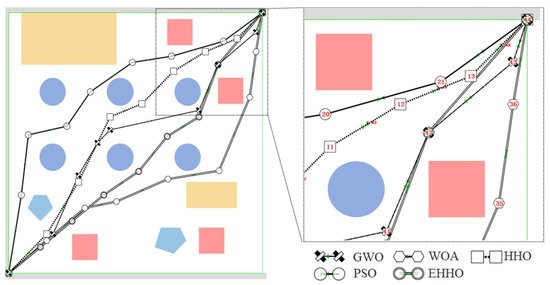
Figure 13.
Comparison of AGV waypoints generated by different path-planning algorithms.
Figure 14.
Path-related parameters (left Y-axis), versus score (right Y-axis, based on overall ranking) (The left axis represents the path length, and the right axis represents the score).
In the AGV deployment experiments, the EHHO algorithm demonstrated comprehensive performance advantages. Compared with the original HHO algorithm, the average path length planned by EHHO was reduced from 28.42 m to 25.35 m, a decrease of 10.81%; the average travel time was reduced from 104.64 s to 92.15 s, a decrease of 11.94%. Compared with other benchmark algorithms, EHHO also exhibited superior performance: path length was reduced by 19.65% and travel time by 19.62% compared with PSO; path length was reduced by 7.66% and travel time by 7.26% compared with GWO; and path length was reduced by 2.97% and travel time by 4.25% compared with WOA. In terms of path smoothness, EHHO achieved the only breakthrough with zero sharp turns, and the average number of turns was reduced to five, the lowest among all algorithms. Based on a comprehensive ranking of the evaluation metrics, EHHO outperformed the second-ranked WOA and the original HHO. The experimental results fully validate the effectiveness of the EHHO algorithm in real industrial scenarios. Through the synergistic effects of the enhanced sine chaotic mapping initialization, the nonlinear energy factor, and the pinhole imaging opposition-based learning strategy, the algorithm not only enhances global optimization capability but also improves path quality, achieving shorter, smoother, and more energy-efficient trajectories for AGVs, thereby providing reliable algorithmic support for improving the efficiency of intelligent warehousing systems.
5. Conclusions
This paper systematically investigates the application of the Harris Hawks Optimization (HHO) algorithm to AGV path-planning problems. To address three core limitations of the standard HHO algorithm when solving such problems—namely, uneven initial population quality, insufficient balance between exploration and exploitation phases, and a tendency to fall into local optima—a comprehensively enhanced Harris Hawks Optimization (EHHO) algorithm is proposed. EHHO integrates three collaboratively operating core strategies: a hybrid initialization strategy based on enhanced sine chaotic mapping improves the quality and diversity of the initial population, generating initial solutions for path planning that are feasible, continuous, and exploratory; a nonlinear escape energy factor replaces the original linear decay mechanism to dynamically balance global exploration and local exploitation, allowing the algorithm to fully explore the solution space in the early iterations and rapidly converge to high-quality solutions in the later stages; and a pinhole imaging opposition-based learning strategy enhances the algorithm’s ability to escape local optima by dynamically generating opposition solutions, effectively avoiding dead ends or locally optimal paths during the path search process.
Through systematic comparisons on 12 classical benchmark functions and the CEC2022 test suite (10-dimensional and 20-dimensional), the advantages of EHHO in convergence accuracy, stability, and robustness are validated. In the classical function tests, EHHO ranks among the top in mean, standard deviation, and best value across multiple unimodal, multimodal, and composite functions, achieving convergence accuracy improvements of several orders of magnitude compared with HHO. In the CEC2022 tests, EHHO ranks first in mean and standard deviation for most functions, and its advantages become more pronounced as problem dimensionality increases. These results fully demonstrate the effectiveness of the nonlinear escape energy factor in balancing search capability, as well as the synergistic effects of the hybrid initialization and opposition-based learning strategies in ensuring population diversity and escaping local optima.
In the validation of path-planning applications, EHHO was deployed on grid maps of varying sizes and complexities and compared with several mainstream algorithms. Experimental results show that EHHO consistently plans shorter and smoother paths across different obstacle densities and map scales, with particularly notable improvements in path length reduction and stability in complex environments. To further verify the engineering applicability of the algorithm, AGV deployment experiments were conducted in a real warehousing scenario. The results indicate that the paths planned by EHHO outperform those of the compared algorithms in key metrics such as path length, travel time, and smoothness, achieving shorter, smoother, and safer trajectories. These findings confirm that the proposed improvement strategies can be effectively translated into tangible engineering performance enhancements.
Overall, EHHO achieves a significant reduction in average path length compared with the original HHO, while the standard deviation of path length is significantly reduced, and both convergence accuracy and stability are effectively improved. The three improvement strategies proposed in this paper synergistically enhance the comprehensive performance of the algorithm from three aspects—namely, the starting point, the process, and the mechanism of optimization. Their effectiveness and reliability are demonstrated not only through mathematical optimization benchmarks but also through practical path-planning experiments. The proposed method provides a feasible optimization framework for intelligent AGV navigation in structured warehouse environments and has potential applicability in practical logistics automation systems.
Although the EHHO algorithm exhibits excellent performance, it still has certain limitations, including the dependence of optimal control parameter selection on problem characteristics, the lack of a dynamic obstacle response mechanism, and a slight increase in runtime due to the opposition-based learning strategy. Future research can focus on improving the generalization capability of parameter adaptation mechanisms and optimizing convergence speed to reduce computational time.
Author Contributions
Conceptualization, C.L. and Y.Z.; methodology, C.L., X.Z. and L.S. software, G.C.; validation, G.C. and Y.Y.; formal analysis, C.L., J.L. (Jiankun Li) and Y.R.; investigation, L.S. and Y.Y.; resources, X.Z., J.L. (Jiankun Li) and J.L. (Jingru Liu); data curation, G.C., Y.Y. and J.L. (Jiankun Li); writing—original draft preparation, G.C.; writing—review and editing, C.L., L.G. and Z.Y.; visualization, G.C., Y.Y. and Y.R.; supervision, Y.Z., X.Z. and Y.R.; project administration, L.S., X.Z. and Z.Y.; funding acquisition, C.L., X.Z. and L.S. All authors have read and agreed to the published version of the manuscript.
Funding
This work was funded by the Jilin Province and Changchun City Major Science and Technology Special, grant number 20230301012ZD.
Institutional Review Board Statement
Not applicable.
Informed Consent Statement
Not applicable.
Data Availability Statement
The original contributions presented in this study are included in the article. Further inquiries can be directed to the corresponding authors.
Conflicts of Interest
Authors Jingru Lui and Lei Gong were employed by the company FAW Tooling Die Manufacturing Co., Ltd. The remaining authors declare that the research was conducted in the absence of any commercial or financial relationships that could be construed as potential conflicts of interest.
Appendix A
A.1. Lyapunov Stability Analysis of the EHHO Algorithm
A.1.1. Lyapunov Function Construction
Let the population position at iteration be
and the global optimum be
. Define a Lyapunov function as
where denotes the Euclidean norm. This function is positive definite and equals zero only when .
A.1.2. Iterative Update Model
The EHHO population updates according to
where includes contributions from the following:
- Enhanced sine chaotic mapping initialization (Equation (6)), ensuring the initial population is uniformly distributed and bounded; Nonlinear convergence factor and escape energy (Equation (8)), which gradually reduce step size during iterations; Pinhole imaging opposition-based learning (Equation (9)), enhancing global search while keeping updates within bounded space.
A.1.3. Lyapunov Difference Analysis
The difference in Lyapunov function between consecutive iterations is
Since the update direction is guided by the global optimum and the step size diminishes over iterations, we have in expectation
Thus,
indicating that the Lyapunov function decreases monotonically in expectation, ensuring gradual convergence toward the optimal region.
A.1.4. Boundedness and Arbitrary Initial Condition Robustness
The enhanced sine chaotic mapping guarantees that the initial population lies within a finite bounded search space Ω. All updates, including opposition-based learning and nonlinear energy-modulated movements, remain within Ω, ensuring that the population trajectories are bounded for any initial condition. Combined with the monotonic decrease of the Lyapunov function in expectation, EHHO exhibits stable convergence behavior, regardless of the initial population distribution.
References
- Ahmad, J.; Wahab, M. Enhancing the safety and smoothness of path planning through an integration of Dijkstra’s algorithm and piecewise cubic Bezier optimization. Expert Syst. Appl. 2025, 289, 128315. [Google Scholar] [CrossRef] [Scilit]
- Luo, Y.; Lin, S.; Wang, Y.; Liang, K. Optimized Path Planning for Autonomous Guided Vehicle Through Fusion of Improved A* and Dynamic Window Approach. IEEE Access 2025, 13, 68577–68586. [Google Scholar] [CrossRef] [Scilit]
- Zhang, Z.; Lu, R.; Zhao, M.; Luan, S.; Bu, M. Robot path planning based on genetic algorithm with hybrid initialization method. J. Intell. Fuzzy Syst. 2022, 42, 2041–2056. [Google Scholar] [CrossRef] [Scilit]
- Wu, C.; Guo, Z.; Zhang, J.; Mao, K.; Luo, D. Cooperative Path Planning for Multiple UAVs Based on APF B-RRT* Algorithm. Drones 2025, 9, 177. [Google Scholar] [CrossRef] [Scilit]
- Xidias, E.; Zacharia, P.; Nearchou, A. Path Planning and scheduling for a fleet of autonomous vehicles. Robotica 2016, 34, 2257–2273. [Google Scholar] [CrossRef] [Scilit]
- Aremu, M.B.; Kabir, I.K.; Ahmed, G.; El-Ferik, S. Autonomous Mobile Robot Path Planning Techniques—A Review: Classical and Heuristic Techniques. IEEE Access 2025, 13, 117999–118022. [Google Scholar] [CrossRef] [Scilit]
- Nan, Y.; Zhu, C.; Li, T.; Zhao, Y.; Guan, A.; Lu, P. Research on obstacle avoidance path planning for multiple UAVs in complex terrain based on an improved ant colony algorithm. Proc. Inst. Mech. Eng. Part G-J. Aerosp. Eng. 2026, 240, 296–309. [Google Scholar] [CrossRef] [Scilit]
- Cheng, Q.; Zhang, Z.; Du, Y.; Zhao, X. Hybrid metaheuristic-driven 3D path planning for UAVs in complex urban environments: A multi-objective fusion framework. Geocarto Int. 2025, 40, 2538099. [Google Scholar] [CrossRef] [Scilit]
- Liu, Y. Global Path Planning Method For Agv Of Warehousing Logistics Based On Improved Ant Colony Algorithm. Int. J. Ind. Eng.-Theory Appl. Pract. 2025, 32, 159–172. [Google Scholar] [CrossRef]
- Ye, F.; Duan, P.; Meng, L.; Xue, L. A hybrid artificial bee colony algorithm with genetic augmented exploration mechanism toward safe and smooth path planning for mobile robot. Biomim. Intell. Robot. 2025, 5, 100206. [Google Scholar] [CrossRef] [Scilit]
- Sun, B.; Li, Y.; Zhang, W. Multipopulation Grey Wolf Optimization for Cooperative Multi-AUV Path Planning in Complex Underwater Environments. IEEE Syst. J. 2025, 19, 837–847. [Google Scholar] [CrossRef] [Scilit]
- Wang, H.; Hao, Z.; Zhang, Y. Research on three-dimensional path planning of unmanned aerial vehicle based on improved Whale Optimization Algorithm. PLoS ONE 2025, 20, e0316836. [Google Scholar] [CrossRef] [Scilit] [PubMed]
- Heidari, A.; Mirjalili, S.; Faris, H.; Aljarah, I.; Mafarja, M.; Chen, H. Harris hawks optimization: Algorithm and applications. Future Gener. Comput. Syst.-Int. J. Escience 2019, 97, 849–872. [Google Scholar] [CrossRef] [Scilit]
- Xu, J.; Chang, X.; Liu, Y.; Wang, X.; Ren, C. Time and energy optimal trajectory planning for freight train cleaning robot based on seventh-degree polynomial interpolation and an improved HHO. Alex. Eng. J. 2025, 122, 165–179. [Google Scholar] [CrossRef] [Scilit]
- Li, S.; Zhang, R.; Ding, Y.; Qin, X.; Han, Y.; Zhang, H. Multi-UAV Path Planning Algorithm Based on BINN-HHO. Sensors 2022, 22, 9786. [Google Scholar] [CrossRef] [Scilit] [PubMed]
- Vikas; Parhi, D. Path planning of humanoid robots on complex terrains using an efficient regression-based chaotic Harris Hawks optimization approach. Robot. Intell. Autom. 2024, 44, 621–633. [Google Scholar] [CrossRef]
- Loganathan, A.; Ahmad, N. A Hybrid HHO-AVOA for Path Planning of a Differential Wheeled Mobile Robot in Static and Dynamic Environments. IEEE Access 2024, 12, 25967–25979. [Google Scholar] [CrossRef] [Scilit]
- Zhang, R.; Li, S.; Ding, Y.; Qin, X.; Xia, Q. UAV Path Planning Algorithm Based on Improved Harris Hawks Optimization. Sensors 2022, 22, 5232. [Google Scholar] [CrossRef] [Scilit] [PubMed]
- Zhang, X.; Gu, G.; Zhao, C. Modified Particle Swarm Optimization for Engineering Optimization Problems and UAV Path Planning. IEEE Access 2025, 13, 83956–83982. [Google Scholar] [CrossRef] [Scilit]

Disclaimer/Publisher’s Note: The statements, opinions and data contained in all publications are solely those of the individual author(s) and contributor(s) and not of MDPI and/or the editor(s). MDPI and/or the editor(s) disclaim responsibility for any injury to people or property resulting from any ideas, methods, instructions or products referred to in the content. |
© 2026 by the authors. Licensee MDPI, Basel, Switzerland. This article is an open access article distributed under the terms and conditions of the Creative Commons Attribution (CC BY) license.