Disturbance Observer-Based Fixed-Time Sliding-Mode Control for Electromechanical Actuators

Abstract

Electromechanical actuators play a pivotal role in aerospace servo systems; however, their high-precision tracking performance is frequently compromised by external disturbances and system nonlinearities. To address these challenges, this paper proposes a disturbance observer-based fixed-time backstepping sliding-mode control strategy. Firstly, the high-order dynamics are decomposed into load and electrical subsystems employing a backstepping control framework. To effectively handle mismatched external disturbances in the load subsystem, a prescribed-time integral sliding-mode observer is designed, which guarantees accurate disturbance estimation within a prescribed time for feedforward compensation. Subsequently, a fixed-time sliding-mode controller incorporating a segmented reaching law is developed. This controller ensures that tracking errors converge to zero within a fixed time, independent of initial system states, while mitigating chattering. Hardware-in-the-loop experimental results demonstrate the superior performance of the proposed strategy. Compared to conventional methods, the proposed controller significantly enhances transient response under step disturbances by reducing the peak deviation by up to 94% and shortening the recovery time by at least 60%. Furthermore, under sustained sinusoidal disturbances and dynamic tracking scenarios, the output fluctuations and tracking errors are attenuated to negligible levels, thereby exhibiting notable improvements over traditional methods.

1. Introduction

Serving as the primary execution mechanisms during aircraft maneuvers, actuators are capable of driving aerodynamic control surfaces, including ailerons, elevators, rudders, flaps, and spoilers, as well as changing the wing camber and thrust vectoring devices, thereby enabling precise control of the aircraft flight path, attitude, airspeed, altitude, and wing configuration [1,2]. Owing to their inherent advantages, such as high torque density and high power density, permanent magnet synchronous motors (PMSMs) [3,4] have been extensively utilized in the engineering development of these servo systems, emerging as the primary driving units for Electromechanical actuators (EMAs) and associated actuation devices. Recent studies [5,6] have investigated this subject from a servo control perspective, aiming to improve the PMSM drive performance and thereby enhance the overall precision and dynamic response of EMAs. Nevertheless, for aerospace EMA applications, conventional servo control schemes may still face limitations when high-accuracy tracking and rapid transient response are required in the presence of transmission flexibility, friction, model uncertainty, and time-varying disturbances [7,8,9]. This motivates the development of more advanced control strategies with improved disturbance-rejection capability and robustness against model parameter perturbations or modeling uncertainties.

The three-loops PID control has been extensively employed in EMA control design due to its simple structure, ease of implementation, and reliable performance [10,11]. It has demonstrated satisfactory effectiveness in many aerospace applications, particularly because the integral term can compensate for constant disturbances and eliminate steady state errors. Nevertheless, the disturbance-rejection capability of conventional PID schemes may still be limited [6,12] under time-varying disturbances.

Disturbances exert a significant influence on the control of EMAs used to manipulate airfoil control surface deflections. To address this issue, contemporary research has proposed a range of disturbance-compensation strategies, including neural network control, model predictive control (MPC), active disturbance rejection methods, and sliding-mode control, with the aim of achieving stable control. Notably, a robust adaptive MPC based on a recurrent neural network (RNN) is proposed in [13], which solves the MPC optimization problem in real time and markedly improves dynamic response, steady-state performance, and disturbance rejection. In [14], a novel variable-structure robust adaptive controller is introduced, employing a two-level interconnected extended-state observer to avoid direct reliance on signals contaminated by noise, thereby enhancing disturbance suppression while improving measurement-noise attenuation. In [15], a disturbance observer-based second-order sliding-mode controller is presented, delivering strong disturbance rejection, significantly mitigating chattering, and improving dynamic performance. Sliding-mode control, noted for its relatively low dependence on model accuracy and strong capacity to handle external disturbances or uncertainties, has thus seen widespread application in servo control. Furthermore, a composite control approach that couples an improved sliding-mode reaching law with an extended disturbance torque observer (DTO) is proposed in [16]. The reaching law adaptively tunes the reaching speed to suppress chattering and shorten convergence time, while the DTO estimates and feedforward method compensates external disturbances, effectively suppressing chatter, accelerating convergence, and markedly enhancing disturbance rejection and dynamic response of the PMSM closed-loop speed control. In [17], a non-singular fast-terminal sliding-mode control framework is presented, coupled with a non-singular fast-terminal sliding-mode disturbance observer to form a comprehensive control strategy that substantially improves disturbance rejection.

However, conventional sliding-mode control suffers from slow convergence and poor transient performance, which has driven extensive research into fixed-time theory-based sliding-mode control. Fixed-time theory guarantees convergence within a fixed time, independent of initial conditions. In [18], a fixed-time observer-based sliding-mode control method is introduced, achieving convergence of the inner and outer loops within a fixed time, robustness to disturbances and parametric uncertainties, and fast and robust speed tracking. In [19], a robust control method based on fixed-time sliding-mode control (FxTSMC) is proposed, combined with an adaptive learning rate neural network state observer, achieving fixed-time convergence, no need for a priori disturbance bounds, and faster convergence with enhanced robustness.

Despite these advances, enhancing the robustness and control performance of EMAs to facilitate aircraft maneuvers remains a formidable challenge. On the one hand, external disturbances inherent in EMAs are frequently mismatched with the control input channel, thereby complicating the implementation of feedforward compensation strategies. Furthermore, relatively few studies have investigated fixed-time position-tracking control for EMA systems while explicitly accounting for external disturbances. Moreover, there is relatively limited research on fixed-time position-tracking control for EMA systems that explicitly account for external disturbances. To address the aforementioned challenges, this paper proposes a disturbance observer-based fixed-time backstepping sliding-mode control strategy for position-tracking control of an electromechanical actuator. The main contributions are summarized as follows:

1.

A fourth-order mathematical model of the EMA subject to external disturbances is established. Based on the backstepping control framework, the model is decomposed into a load-side subsystem and an electrical-side subsystem. A prescribed-time integral sliding-mode observer is designed to accurately estimate the mismatched external disturbance and compensate for it in the virtual control law.

2.

Within the backstepping control framework, a fixed-time sliding-mode control scheme is developed. Position-tracking control laws based on segmented reaching law are designed separately for the load-side subsystem and the electrical-side subsystem, ensuring that the control errors converge within fixed time.

3.

Hardware-in-the-loop experiments are conducted to validate the effectiveness of the proposed disturbance observer-based fixed-time backstepping sliding-mode control strategy.

The remainder of this paper is organized as follows. The model of EMA and preliminaries are developed in Section 2, and the control scheme is designed in Section 3. Detailed hardware-in-the-loop experimental results are provided in Section 4, which are followed by conclusions in Section 5.

2. EMA Model Development and Preliminaries

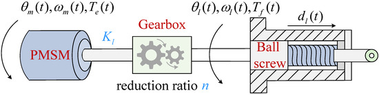
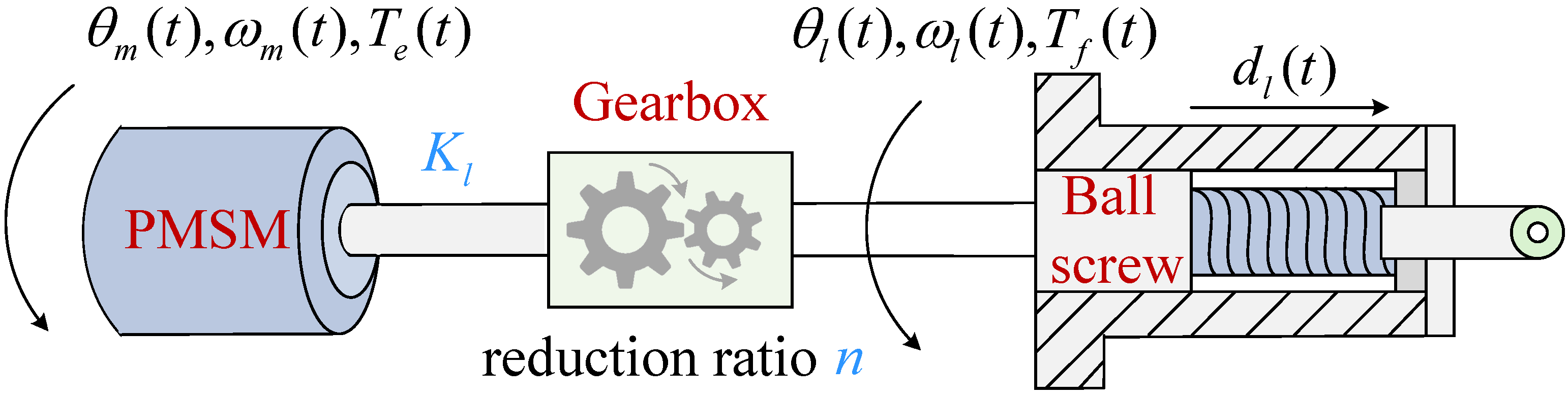
The considered plant is a ball-screw-driven aerospace EMA used for flight control type actuation, which typically consists of an electrical subsystem and a mechanical transmission and load subsystem. The latter is defined with respect to the former and represents the equivalent mechanical subsystem coupled to the PMSM side. The PMSM in the electrical subsystem drives the mechanical transmission through a gearbox, and the resulting rotation is converted by a ball-screw mechanism into linear displacement at the end. As shown in Figure 1, this configuration represents a typical schematic of an EMA.

Figure 1. Schematic diagram of an EMA.

2.1. Electrical Subsystem

The electrical dynamics of the PMSM are established in the $d-q$ (direct-quadrature) synchronous rotating reference frame, the d-axis is aligned with the rotor magnetic flux linkage, and the q-axis is orthogonal to it. In this frame, the electromagnetic torque of a PMSM comprises two components, namely, the permanent-magnet torque and the reluctance torque. The torque equation can be expressed as [20]

$$\begin{array}{c}\hfill T_e={\displaystyle \frac{3}{2}}{n}_p\left({\psi }_f{i}_q+(L_d-L_q)i_d{i}_q\right)\end{array}$$

(1)

where $T_e$ denotes the electromagnetic torque, $n_p$ is the number of pole pairs, ${\psi }_f$ represents the permanent-magnet flux linkage; $L_d$ and $L_q$ are the inductances of the d-axis and the q-axis, respectively; and $i_d$ and $i_q$ are the corresponding currents of the d-axis and q-axis. In this study, the d-axis and q-axis inductances are assumed to be equal, and a field-oriented control strategy with $i_d=0$ is adopted. Under these conditions, the reluctance torque term vanishes, and thus (1) can be rewritten as

$$\begin{array}{c}\hfill T_e={\displaystyle \frac{3}{2}}{n}_p{\psi }_f{i}_q\triangleq K_t{i}_q\end{array}$$

(2)

where $K_t$ denotes the torque constant. The control-oriented simplified mechanical equation, in which the electromagnetic torque overcomes the load torque, can be expressed as [5,8,21]

$$\begin{array}{c}\hfill J_m{\ddot{\theta }}_m+B_m{\dot{\theta }}_m=T_e-T_l\end{array}$$

(3)

where $J_m$ denotes the rotor moment of inertia, $B_m$ is the damping coefficient. ${\theta }_m$ represents the rotor angular displacement and $T_l$ is the load torque.

2.2. Mechanical Transmission and Load Subsystem

The mechanical transmission and load subsystem considered describes the equivalent output-side mechanical dynamics associated with the ball-screw stage of the benchmark model, which can be called load-side subsystem in this study. The torque generated by the PMSM is transmitted through the reduction gearbox to the ball-screw stage, where it is converted into the linear output displacement. In the present benchmark model, the model is established up to this linear output stage. The corresponding equation of motion can be expressed as

$$\begin{array}{c}\hfill J_l{\ddot{\theta }}_l+B_l{\dot{\theta }}_l=n{T}_l-T_f\end{array}$$

(4)

where $J_l$ and $B_l$ denote the reflected inertia and viscous friction referred to the load-side coordinate respectively. ${\theta }_l$ represents the angular displacement at the output terminal of the gearbox. n denotes the reduction ratio of the gearbox. $T_f$ denotes a lumped disturbance torque referred to the output terminal of the gearbox, which includes external load variation, coulomb friction and other unmodeled resistive effects. The dynamics of the motor and the load are linked via the torsional torque of the transmission shaft [22]. According to Hooke’s law, the torque is obtained by multiplying the angular difference between the two ends by the torsional stiffness coefficient. Therefore, the load torque $T_l$ can be expressed as

$$\begin{array}{c}\hfill T_l=K_l({\theta }_m-n{\theta }_l)\end{array}$$

(5)

where the elastic effects associated with the gear meshing, thrust bearings, and transmission path are equivalent to a concentrated torque stiffness $K_l$, which is placed at the transmission chain between the PMSM output side and the gearbox. ${\theta }_l$ is then transformed into the linear displacement $d_l$ of the ball screw, which can be formulated as

$$\begin{array}{c}\hfill d_l={\displaystyle \frac{P_h}{2\pi }}{\theta }_l.\end{array}$$

(6)

where $P_h$ is the ball-screw lead.

2.3. Preliminaries Model of EMA

According to (3) and (4), the state variables are selected as $x=[x_1,x_2,x_3,x_4]=[{\theta }_l,{\omega }_l,{\theta }_m,{\omega }_m]$, where ${\omega }_l$ and ${\omega }_m$ denote the load angular velocity and the motor rotor angular velocity, respectively. The full-order mathematical model of the electromechanical actuator can be obtained as

$$\left\{\begin{array}{c}{\dot{x}}_1=x_2\hfill \\ {\dot{x}}_2=-{\displaystyle \frac{n^2{K}_l}{J_l}}{x}_1-{\displaystyle \frac{B_l}{J_l}}{x}_2+{\displaystyle \frac{n{K}_l}{J_l}}{x}_3+\epsilon \hfill \\ {\dot{x}}_3=x_4\hfill \\ {\dot{x}}_4={\displaystyle \frac{n{K}_l}{J_m}}{x}_1-{\displaystyle \frac{K_l}{J_m}}{x}_3-{\displaystyle \frac{B_m}{J_m}}{x}_4+{\displaystyle \frac{K_t}{J_m}}u\hfill \\ y=x_1\hfill \end{array}\right.$$

(7)

where $u=i_q$, $y={\displaystyle \frac{2\pi }{P_h}}{d}_l$, and $\epsilon =-{\displaystyle \frac{T_f}{J_l}}$. Through angle sensors installed on the PMSM side and an additional position sensor specifically equipped on the load side, the angular displacement and angular velocity of both the PMSM and the load can be directly measured.

2.4. Preliminaries

Lemma 1

([23]). If $\delta >1$, $z_i\ge 0$, and $0<\varsigma \le 1$, then the two following inequalities are valid:

$$\begin{array}{c}\hfill {\displaystyle \sum _{i=1}^n}{z}_i^{\varsigma }\ge {\left({\displaystyle \sum _{i=1}^n}{z}_i\right)}^{\varsigma }\end{array}$$

(8)

$$\begin{array}{c}\hfill {\displaystyle \sum _{i=1}^n}{z}_i^{\delta }\ge n^{1-\delta }{\left({\displaystyle \sum _{i=1}^n}{z}_i\right)}^{\delta }.\end{array}$$

(9)

Lemma 2

([24]). Given the specified nonlinear continuous system

$$\begin{array}{c}\hfill \dot{g}=-w_1{⟨g⟩}^{\chi }-w_2\mathrm{sign}\left(g\right)\end{array}$$

(10)

where $g\left(0\right)=g_0$, $⟨g⟩={\left|g\right|}^{\chi }\mathrm{sign}\left(g\right)$, $\chi ={\displaystyle \frac{m+n}{2}}+{\displaystyle \frac{m-n}{2}}\mathrm{sign}\left(\right|g|-1)$, $w_1,w_2>0$, $m>1$, and $0<n<1$. Then, the system (10) converges to zero within fixed time T, and the upper bound of the convergence time can be expressed as

$$\begin{array}{c}\hfill T_{max}=\frac{2^{\frac{m-1}{2}}}{w_1^{\frac{m+1}{2}}(m-1)}{\left(w_1^{\frac{2}{m+1}}+w_2^{\frac{2}{m+1}}\right)}^{\frac{1-m}{2}}+\frac{1}{w_2(1-n)}ln\left({\displaystyle \frac{w_1+w_2}{w_1}}\right).\end{array}$$

(11)

Lemma 3

([24]). For an arbitrary-order integrator system:

$$\left\{\begin{array}{c}{\dot{g}}_1=g_2,\hfill \\ {\dot{g}}_2=g_3,\hfill \\ ⋮\hfill \\ {\dot{g}}_n=-{\displaystyle {\sum }_{i=1}^n}{k}_i{G}_i\left(g_i\left(t\right)\right)\hfill \end{array}\right.$$

(12)

where $G_i\left(g_i\left(t\right)\right)={⟨g_i⟩}^{{\alpha }_i}+⟨g_i⟩+{⟨g_i⟩}^{{\beta }_i}$, $⟨g_i⟩={\left|g_i\right|}^{\chi }\mathrm{sign}\left(g_i\right)$, ${\alpha }_i={\displaystyle \frac{n\alpha }{n-(i-1)(1-\alpha )}}$, ${\beta }_i={\displaystyle \frac{n\beta }{n-(i-1)(1-\beta )}}$, and α, β that satisfy $\alpha \in (1-{ϵ}_{\alpha },1),\beta \in (1,1+{ϵ}_{\beta })$ where ${ϵ}_{\alpha }$ and ${ϵ}_{\beta }$ are small constants. If $k_i$ are selected to guaranty the Hurwitz matrix (13), then the system (12) is fixed-time stable:

$$\begin{array}{c}\hfill H=\left[\begin{array}{ccccc}0& \frac{1}{3}& 0& \dots & 0\\ 0& 0& \frac{1}{3}& \dots & 0\\ ⋮& ⋮& ⋮& \ddots & ⋮\\ 0& 0& 0& \dots & \frac{1}{3}\\ -k_1& -k_2& -k_3& \dots & -k_n\end{array}\right]\end{array}$$

(13)

3. Composite Controller Design for EMA

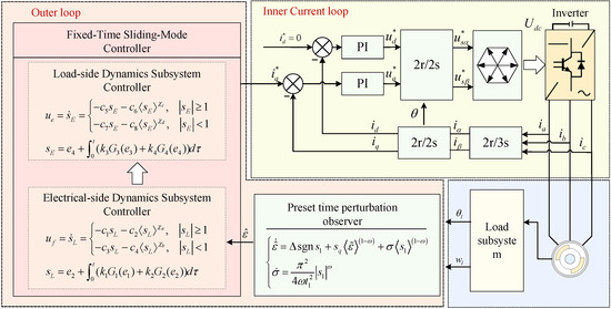
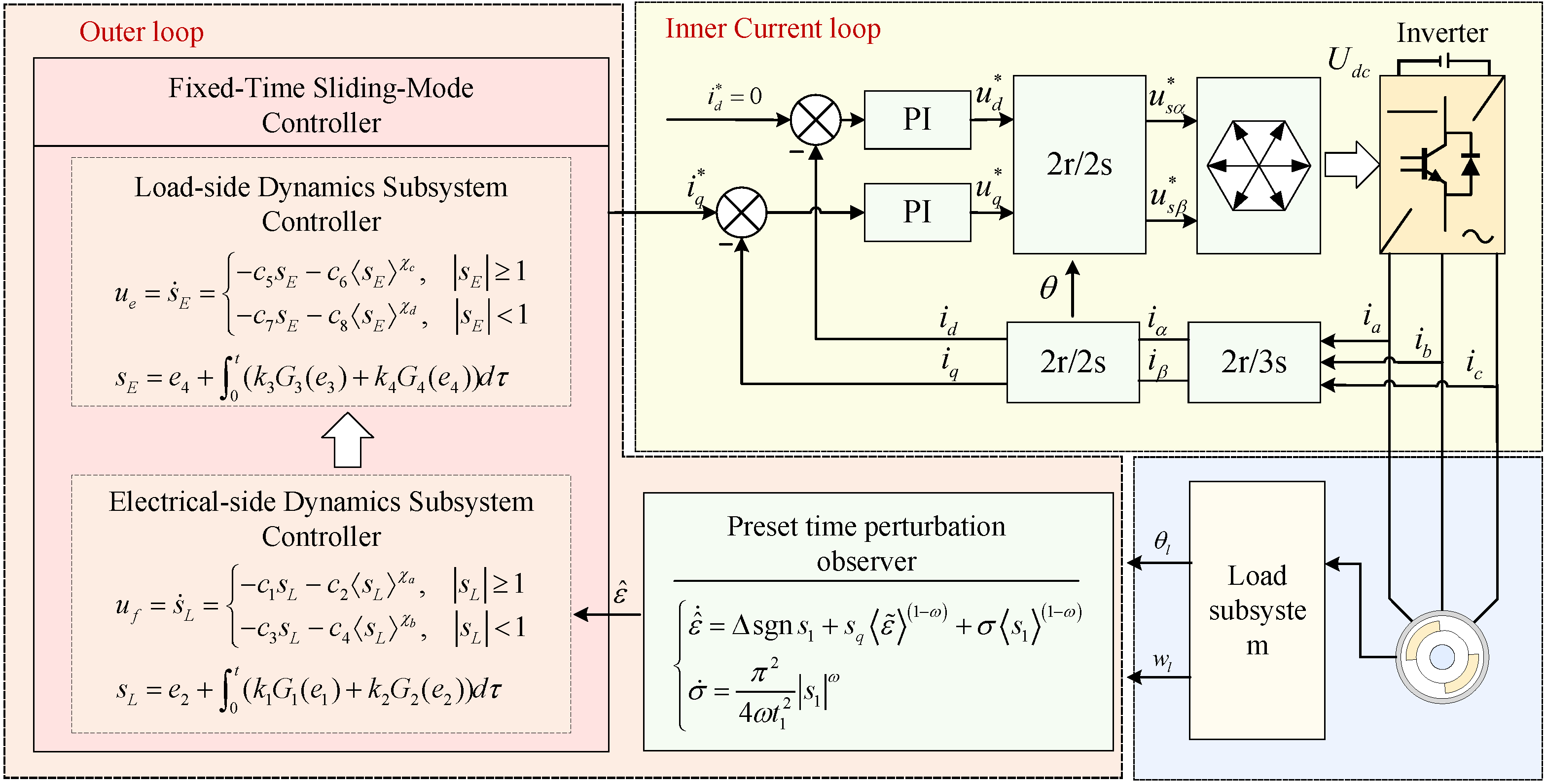
The proposed control structure consists of two loops, as illustrated in Figure 2. In the outer loop, a backstepping-based control framework is developed. Based on the feedback information from the electrical and load subsystems, a fixed-time sliding-mode controller is designed to calculate the control input $i_q^{*}$. In the inner current loop, PI controllers are employed to make $i_q$ track the desired q-axis current $i_q^{*}$ generated by the outer-loop controller and make $i_d$ track the desired d-axis current $i_d=0$.

Figure 2. Schematic of the proposed control method.

Since the sampling frequency of the inner current loop is much higher than that of the outer loop, the two loops are controlled independently. This work focuses on the design of the outer-loop control method, and the current is assumed to be accurately controlled.

3.1. Prescribed-Time Integral Sliding-Mode Observer

Since a disturbance $\epsilon$ exists in the load-side dynamics subsystem, an adaptive prescribed-time sliding-mode observer is designed as follows to achieve accurate disturbance estimation:

$$\left\{\begin{array}{c}\dot{\widehat{\epsilon }}=\Delta \mathrm{sign}{s}_1+s_q{⟨\tilde{\epsilon }⟩}^{(1-\varpi )}+\sigma {⟨s_1⟩}^{(1-\varpi )}\hfill \\ \dot{\sigma }={\displaystyle \frac{{\pi }^2}{4\varpi t_1^2}}{\left|s_1\right|}^{\varpi }\hfill \end{array}\right.$$

(14)

where $\widehat{\epsilon }$ denotes the estimate of $\epsilon$, $\Delta$ denotes the known upper bound of the disturbance $\epsilon$ and $\sigma$ denotes the adaptive parameter, with $\sigma \left(0\right)=0$. $\varpi$ is a design parameter which satisfies $\varpi \in (0,1)$, and $t_1$ is the prescribed time. $s_q$ denotes the component of the integral sliding-model surface, with $s_q\left(0\right)=0$; $s_1$ is the designed sliding-model surface, which can be expressed as

$$\left\{\begin{array}{c}{s}_1=\tilde{\epsilon }+{\int }_0^t{s}_q{⟨\tilde{\epsilon }⟩}^{(1-\varpi )}d\tau \hfill \\ \dot{s_q}={\displaystyle \frac{{\pi }^2}{4\varpi t_2^2}}{\left|\tilde{\epsilon }\right|}^{\varpi }\hfill \end{array}\right.$$

(15)

where $t_2$ denotes the convergence time of the sliding-model surface error to be designed and $\tilde{\epsilon }$ denotes the disturbance estimation error with

$$\begin{array}{c}\hfill \tilde{\epsilon }={\dot{x}}_2-f\left(x\right)-\widehat{\epsilon },\end{array}$$

(16)

where $f\left(x\right)=-{\displaystyle \frac{n^2{K}_l}{J_l}}{x}_1-{\displaystyle \frac{B_l}{J_l}}{x}_2+{\displaystyle \frac{n{K}_l}{J_l}}{x}_3$.

In order to prove that the designed disturbance observer can drive the estimation error of the disturbance $\tilde{\epsilon }$ to converge to 0 within the prescribed time $T_0=t_1+t_2$. Define the Lyapunov function $V_0$ as

$$\begin{array}{c}\hfill V_0={\displaystyle \frac{1}{\varpi }}{\left|s_1\right|}^{\varpi }\end{array}$$

(17)

Taking the time derivative of $V_0$, one obtains the following:

$$\begin{array}{c}\hfill {\dot{V}}_0=s_1^{\varpi -1}{\dot{s}}_1\end{array}$$

(18)

By combining (14), (15) and (18), one obtains

$$\begin{array}{c}{\dot{V}}_0=s_1^{\varpi -1}\left(\dot{\tilde{\epsilon }}+s_q{⟨\tilde{\epsilon }⟩}^{1-\varpi }\right)\hfill \\ =s_1^{\varpi -1}\left(\dot{\epsilon }-\dot{\widehat{\epsilon }}+s_q{⟨\tilde{\epsilon }⟩}^{1-\varpi }\right)\hfill \\ =s_1^{\varpi -1}(\dot{\epsilon }-\Delta \mathrm{sgn}{s}_1-s_q{⟨\tilde{\epsilon }⟩}^{(1-\varpi )}-\sigma {⟨s_1⟩}^{(1-\varpi )}+s_q{⟨\tilde{\epsilon }⟩}^{(1-\varpi )})\hfill \\ =s_1^{\varpi -1}(\dot{\epsilon }-\Delta \mathrm{sgn}{s}_1-\sigma {⟨s_1⟩}^{(1-\varpi )})\hfill \\ \le -\sigma .\hfill \end{array}$$

(19)

Introduce a time-varying positive function $H\left(t\right)$ such that $\dot{V_0}$ satisfies

$$\begin{array}{c}\hfill \dot{V_0}\left(t\right)=-\sigma -H\left(t\right)\end{array}$$

(20)

Then, applying the Laplace transform to (20), one obtains the following:

$$s{V}_0\left(s\right)-V_0\left(0\right)=-\sigma \left(s\right)-H\left(s\right)$$

(21)

Taking the Laplace transform of the second equation in (14) and assuming the initial condition $\sigma \left(0\right)=0$, we have

$$s\sigma \left(s\right)={\displaystyle \frac{{\pi }^2}{4t_1^2}}{V}_0\left(s\right)$$

(22)

Solving (22) for $\sigma \left(s\right)$ yields

$$\sigma \left(s\right)={\displaystyle \frac{{\pi }^2}{4s{t}_1^2}}{V}_0\left(s\right)$$

(23)

Substituting this result into (21) to eliminate $\sigma \left(s\right)$ gives

$$s{V}_0\left(s\right)-V_0\left(0\right)=-\left({\displaystyle \frac{{\pi }^2}{4s{t}_1^2}}{V}_0\left(s\right)\right)-H\left(s\right)$$

(24)

By rearranging the terms, $V_0\left(s\right)$ can be finally expressed as

$$V_0\left(s\right)={\displaystyle \frac{s}{s^2+{\displaystyle \frac{{\pi }^2}{4t_1^2}}}}{V}_0\left(0\right)-{\displaystyle \frac{s}{s^2+{\displaystyle \frac{{\pi }^2}{4t_1^2}}}}H\left(s\right)$$

(25)

Furthermore, applying the inverse Laplace transform to (25) and using trigonometric identities, one obtains the following:

$$\begin{array}{c}\hfill V_0=V_0\left(0\right)cos\left({\displaystyle \frac{\pi }{2t_1}}t\right)-H\left(t\right)cos\left({\displaystyle \frac{\pi }{2t_1}}t\right)\le V_0\left(0\right)cos\left({\displaystyle \frac{\pi }{2t_1}}t\right)\end{array}$$

(26)

It follows that $V_0$ converges to 0 within $t_1$. Therefore, the sliding surface can be reached within the prescribed time $t_1$. At this point, ${\dot{s}}_1=0$, according to (15), and the error convergence system can be expressed as

$$\begin{array}{c}\hfill \dot{\tilde{\epsilon }}=-s_q{⟨\tilde{\epsilon }⟩}^{(1-\varpi )}.\end{array}$$

(27)

Define the Lyapunov function $V_1$ as

$$\begin{array}{c}\hfill V_1={\displaystyle \frac{1}{\varpi }}{\left|\tilde{\epsilon }\right|}^{\varpi }\end{array}$$

(28)

Taking the time derivative of $V_1$, one obtains

$$\begin{array}{c}\hfill \dot{V_1}=-s_q\end{array}$$

(29)

Combining (14) and taking the Laplace transform of (29), one obtains the following:

$$\begin{array}{c}\hfill V_1\left(s\right)={\displaystyle \frac{s}{s^2+{\displaystyle \frac{{\pi }^2}{4t_2^2}}}}{V}_1\left(0\right)\end{array}$$

(30)

where $V_1\left(0\right)$ represents the initial value of $V_1$. It can be proven that $V_1$ converges to zero within $t_2$. Moreover, since $\dot{V_1}$ is negative definite, the system achieves prescribed-time stability within $t_2$. Therefore, the error convergence system (27) converges within $t_2$. Consequently, the estimation error of the (14) achieves prescribed-time convergence, with an overall convergence time bounded by $T_o=t_1+t_2$.

3.2. Fixed-Time Sliding-Mode Controller Design

To suppress the influence of external disturbances on the precise tracking of desired commands by the load control surface, this section designs the control laws for the load-side dynamics subsystem and the electrical-side dynamics subsystem based on a fixed-time control strategy. Specifically, following the idea of backstepping sliding-mode control, a virtual control input $x_{3r}$ is designed, and the disturbance estimation obtained in Section 3.1 is incorporated into the virtual control input for compensation, so that $x_1$ in the load-side dynamics subsystem can accurately track the desired control surface displacement within fixed time. Furthermore, a control input u is designed for the electrical subsystem, thereby ensuring in the inner loop that the PMSM rotor angle can track the designed virtual control input $x_{3r}$ within a fixed time.

3.2.1. Load-Side Dynamics Subsystem Controller Design

Considering the load subsystem

$$\begin{array}{c}\hfill \left\{\begin{array}{cc}{\dot{x}}_1=x_2\hfill & \\ {\dot{x}}_2=-{\displaystyle \frac{n^2{K}_l}{J_l}}{x}_1-{\displaystyle \frac{B_l}{J_l}}{x}_2+{\displaystyle \frac{n{K}_l}{J_l}}{x}_3+\epsilon \hfill & \end{array}\right.\end{array}$$

(31)

the fixed-time integral terminal sliding surface is defined as

$$\begin{array}{c}\hfill s_L=e_2+{\int }_0^t\left(k_1{G}_1\left(e_1\right)+k_2{G}_2\left(e_2\right)\right)d\tau \end{array}$$

(32)

with

$$\left\{\begin{array}{c}{G}_1\left(e_1\right)={⟨e_1⟩}^{{\alpha }_a}+⟨e_1⟩+{⟨e_1⟩}^{{\beta }_a}\hfill \\ G_2\left(e_2\right)={⟨e_2⟩}^{\frac{2{\alpha }_a}{{\alpha }_a+1}}+⟨e_2⟩+{⟨e_2⟩}^{\frac{2{\beta }_a}{{\beta }_a+1}},\hfill \end{array}\right.$$

(33)

where $e_1$ and $e_2$ denote the tracking errors of the load angular displacement and angular velocity, respectively. The parameters ${\alpha }_a$, ${\beta }_a$ represent the sliding surface coefficients, which satisfy ${\alpha }_a\in (1-{ϵ}_{\alpha },1),{\beta }_a\in (1,1+{ϵ}_{\beta })$ where ${ϵ}_{\alpha }$ and ${ϵ}_{\beta }$ are small constants. $k_1$ and $k_2$ are gain coefficients.

The fixed-time sliding-mode reaching law is designed as

$$\begin{array}{c}\hfill u_f={\dot{s}}_L=\left\{\begin{array}{cc}-c_1{s}_L-c_2{⟨s_L⟩}^{{\chi }_a},\hfill & |s_L|\ge 1\hfill \\ -c_3{s}_L-c_4{⟨s_L⟩}^{{\chi }_b},\hfill & |s_L|<1\hfill \end{array}\right.\end{array}$$

(34)

where $c_1+c_2=c_3+c_4$, ${\chi }_a>1$ and $0<{\chi }_b<1$. By combining Equations (32) and (34), one obtains

$$\begin{array}{cc}\hfill {\dot{s}}_L& =-{\displaystyle \frac{n^2{K}_l}{J_l}}{x}_1-{\displaystyle \frac{B_l}{J_l}}{x}_2+{\displaystyle \frac{n{K}_l}{J_l}}{x}_3+\epsilon -\ddot{x_d}+k_1\left(e_1\right)G_1\left(e_1\right)+k_2\left(e_2\right)G_2\left(e_2\right)\hfill \\ \hfill & =u_f\hfill \end{array}$$

(35)

where $\ddot{x_d}=\ddot{y_d}={\displaystyle \frac{\ddot{l}}{k}}$. By replacing the external disturbance in (35) with the estimated value given in (14), the virtual control input can be obtained as

$$\begin{array}{c}\hfill x_{3r}={\displaystyle \frac{J_l}{n{K}_l}}(\ddot{x_d}+{\displaystyle \frac{n^2{K}_l}{J_l}}{x}_1+{\displaystyle \frac{B_l}{J_l}}{x}_2-\widehat{\epsilon }-k_1\left(e_1\right)G_1\left(e_1\right)-k_2\left(e_2\right)G_2\left(e_2\right)+u_f).\end{array}$$

(36)

In order to prove that the designed virtual control law $x_{3r}$ can drive the state $x_1$ to track the desired signal $x_d$ within fixed time, we begin by proving that the proposed piecewise-approaching law drives the system to the sliding surface in a fixed time. Let the initial value of the sliding surface be $s_{L0}$. Consider the case $s_L>0$, it follows that when $s_{L0}\ge 1$, the reaching law guides the state from the initial value $s_{L0}$ down to 1, and subsequently from 1 to 0, in two successive phases from (34). When $s_{L0}<1$, the proposed approaching law requires only a single segment of motion for the system to reach the sliding surface. The present discussion will address these two cases separately.

For $s_{L0}\ge 1$, if $s_L\in [1,s_{L0})$, according to (34), one obtains

$$\begin{array}{c}\hfill {\dot{s}}_L+c_1{s}_L+c_2{s}_L^{{\chi }_a}=0\end{array}$$

(37)

Solving (37) yields

$$\begin{array}{c}\hfill s_L^{1-{\chi }_a}=(s_{L0}^{1-{\chi }_a}+{\displaystyle \frac{c_2}{c_1}})e^{c_1({\chi }_a-1)t}-{\displaystyle \frac{c_2}{c_1}}\end{array}$$

(38)

Hence, the convergence time up to reaching $s_L=1$ can be expressed as

$$\begin{array}{cc}\hfill t_3& ={\displaystyle \frac{1}{c_1({\chi }_a-1)}}\left[ln(c_1+c_2)-ln\left(c_1{s}_{L0}^{1-{\chi }_a}+c_2\right)\right]\hfill \\ & \le {\displaystyle \frac{1}{c_1({\chi }_a-1)}}\left({\displaystyle \frac{c_1+c_2}{c_1{s}_{L0}^{1-{\chi }_a}+c_2}}-1\right)\hfill \\ & ={\displaystyle \frac{1-s_{L0}^{1-{\chi }_a}}{({\chi }_a-1)c_1{s}_{L0}^{1-{\chi }_a}+c_2}}\hfill \\ & <{\displaystyle \frac{1}{c_2({\chi }_a-1)}}\hfill \end{array}$$

(39)

If $s_L\in (0,1)$, one obtains

$$\begin{array}{c}\hfill {\dot{s}}_L+c_3{s}_L+c_4{s}_L^{{\chi }_b}=0\end{array}$$

(40)

By solving the differential equation, the convergence time up to reaching $s_L=0$ can be expressed as

$$\begin{array}{c}\hfill t_4={\displaystyle \frac{1}{c_3(1-{\chi }_b)}}\left[ln(c_3+c_4)-ln{c}_4\right]\end{array}$$

(41)

Therefore, when $s_{L0}\ge 1$, the convergence time $T_1$ is within ${\displaystyle \frac{1}{c_2({\chi }_a-1)}}+{\displaystyle \frac{1}{c_3(1-{\chi }_b)}}\left[ln(c_3+c_4)-ln{c}_4\right]$

For $s_{L0}<1$, according to (34), one obtains

$$\begin{array}{c}\hfill {\dot{s}}_L+c_3{s}_L+c_4{s}_L^{{\chi }_b}=0\end{array}$$

(42)

By solving the differential equation, the convergence time can be expressed as

$$\begin{array}{cc}\hfill t_5& ={\displaystyle \frac{1}{c_3(1-{\chi }_b)}}\left[ln(c_3{s}_{L0}^{1-{\chi }_b}+c_4)-ln{c}_4\right]\hfill \\ & \le {\displaystyle \frac{s_{L0}^{1-{\chi }_b}}{c_4(1-{\chi }_b)}}\hfill \\ & <{\displaystyle \frac{1}{c_4(1-{\chi }_b)}}\hfill \end{array}$$

(43)

Therefore, when $s_{L0}<1$, the convergence time $T_1$ is within ${\displaystyle \frac{1}{c_4(1-{\chi }_b)}}$. Subsequently, it is proven that during the sliding-mode phase, i.e., when $s_L\equiv 0$, the system error converges in fixed time. From (32), it follows that

$$\begin{array}{c}\hfill \left\{\begin{array}{c}{\dot{e}}_1=e_2\hfill \\ {\dot{e}}_2=-k_1{G}_1\left(e_1\right)-k_2{G}_2\left(e_2\right)\hfill \end{array}\right.\end{array}$$

(44)

According to Lemma 3, the error convergence time $T_2$ during sliding-mode control satisfies

$$\begin{array}{c}\hfill T_2\le {\displaystyle \frac{4({\beta }_a+1){\lambda }_{max}\left(P_a\right)}{({\beta }_a-1){\lambda }_{min}\left(Q_a\right){\lambda }_{min}{\left(P_a\right)}^{\frac{{\beta }_a-1}{2{\beta }_a+2}}}}+{\displaystyle \frac{8({\alpha }_a+1){\left({\lambda }_{max}\left(P_a\right)\right)}^{\frac{5+3{\alpha }_a}{4({\alpha }_a+1)}}}{{\lambda }_{min}\left(Q_a\right)(1-{\alpha }_a)}}\end{array}$$

(45)

where the ${\lambda }_{max}$ and ${\lambda }_{min}$ represent the maximum and minimum eigenvalues of the respective matrices and the matrices $P_a$ and $Q_a$ satisfy $P_a{H}_a+H_a^T{P}_a=-Q_a$ with $H_a=\left[\begin{array}{cc}0& {\displaystyle \frac{1}{3}}\\ -k_1& -k_2\end{array}\right].$ Consequently, for the load-side subsystem, the convergence time is within $T_0+T_1+T_2$.

3.2.2. Electrical-Side Dynamics Subsystem Controller Design

Considering the electrical-side dynamics subsystem

$$\left\{\begin{array}{c}{\dot{x}}_3=x_4\hfill \\ {\dot{x}}_4={\displaystyle \frac{n{K}_l}{J_m}}{x}_1-{\displaystyle \frac{K_l}{J_m}}{x}_3-{\displaystyle \frac{B_m}{J_m}}{x}_4+{\displaystyle \frac{K_t}{J_m}}u\hfill \end{array}\right.$$

(46)

the fixed-time integral terminal sliding surface is defined as

$$\begin{array}{c}\hfill s_E=e_4+{\int }_0^t\left(k_3{G}_3\left(e_3\right)+k_4{G}_4\left(e_4\right)\right)d\tau \end{array}$$

(47)

with

$$\left\{\begin{array}{c}{G}_3\left(e_3\right)={⟨e_3⟩}^{{\alpha }_b}+⟨e_3⟩+{⟨e_3⟩}^{{\beta }_b}\hfill \\ G_4\left(e_4\right)={⟨e_4⟩}^{\frac{2{\alpha }_b}{{\alpha }_b+1}}+⟨e_4⟩+{⟨e_4⟩}^{\frac{2{\beta }_b}{{\beta }_b+1}},\hfill \end{array}\right.$$

(48)

where $e_3$ and $e_4$ denote the tracking errors of the PMSM angular displacement and angular velocity with $e_3=x_3-x_{3r}$ and $e_4=x_4-\dot{x_{3r}}$, respectively. $k_3$ and $k_4$ are gain coefficients. ${\alpha }_b$, ${\beta }_b$ represent the sliding surface coefficients, which satisfy ${\alpha }_b\in (1-{ϵ}_{\alpha },1),{\beta }_b\in (1,1+{ϵ}_{\beta })$ where ${ϵ}_{\alpha }$ and ${ϵ}_{\beta }$ are small constants. The fixed-time sliding-mode reaching law is designed as

$$\begin{array}{c}\hfill u_e={\dot{s}}_E=\left\{\begin{array}{cc}-c_5{s}_E-c_6{⟨s_E⟩}^{{\chi }_c},\hfill & |s_E|\ge 1\hfill \\ -c_7{s}_E-c_8{⟨s_E⟩}^{{\chi }_d},\hfill & |s_E|<1\hfill \end{array}\right.\end{array}$$

(49)

where $c_5+c_6=c_7+c_8$, ${\chi }_c>1$ and $0<{\chi }_d<1$. Then, by combining Equations (47) and (49), one obtains

$$\begin{array}{cc}\hfill {\dot{s}}_E& ={\displaystyle \frac{n{K}_l}{J_m}}{x}_1-{\displaystyle \frac{K_t}{J_m}}{x}_3-{\displaystyle \frac{B_m}{J_m}}{x}_4+{\displaystyle \frac{K_e}{J_m}}u-{\ddot{x}}_{3r}+k_3\left(e_3\right)G_3\left(e_3\right)+k_4\left(e_4\right)G_4\left(e_4\right)\hfill \\ \hfill & =u_e\hfill \end{array}$$

(50)

Therefore, the control law u can be expressed as

$$\begin{array}{cc}\hfill u& ={\displaystyle \frac{J_m}{K_e}}(-{\displaystyle \frac{n{K}_l}{J_m}}{x}_1+{\displaystyle \frac{K_l}{J_m}}{x}_3+{\displaystyle \frac{B_m}{J_m}}{x}_4+\ddot{x_{3r}}-k_3{G}_3\left(e_3\right)\hfill \\ & -k_4{G}_4\left(e_4\right)+u_e)\hfill \end{array}$$

(51)

The convergence time is within $T_3+T_4$, where

$$\begin{array}{cc}\hfill T_3& \le \left\{\begin{array}{cc}{\displaystyle \frac{1}{c_6({\chi }_c-1)}}+{\displaystyle \frac{1}{c_7(1-{\chi }_d)}}\left[ln(c_7+c_8)-ln{c}_8\right],\hfill & \hfill |s_{E0}|\ge 1\\ {\displaystyle \frac{1}{c_8(1-{\chi }_d)}},\hfill & \hfill |s_{E0}|<1\end{array}\right.\hfill \\ \hfill T_4& \le {\displaystyle \frac{4({\beta }_b+1){\lambda }_{max}\left(P_b\right)}{({\beta }_b-1){\lambda }_{min}\left(Q_b\right){\lambda }_{min}{\left(P_b\right)}^{\frac{{\beta }_b-1}{2{\beta }_b+2}}}}+{\displaystyle \frac{8({\alpha }_b+1){\left({\lambda }_{max}\left(P_b\right)\right)}^{\frac{5+3{\alpha }_b}{4({\alpha }_b+1)}}}{{\lambda }_{min}\left(Q_b\right)(1-{\alpha }_b)}}\hfill \end{array}$$

(52)

where the matrices $P_b$ and $Q_b$ satisfy $P_b{H}_b+H_b^T{P}_b=-Q_b$ with $H_b=\left[\begin{array}{cc}0& {\displaystyle \frac{1}{3}}\\ -k_3& -k_4\end{array}\right]$; the proof follows similarly to the load-side dynamics subsystem and is omitted due to space limitations.

4. Results and Discussion

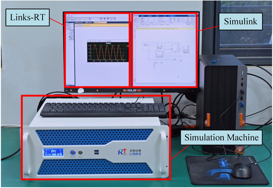
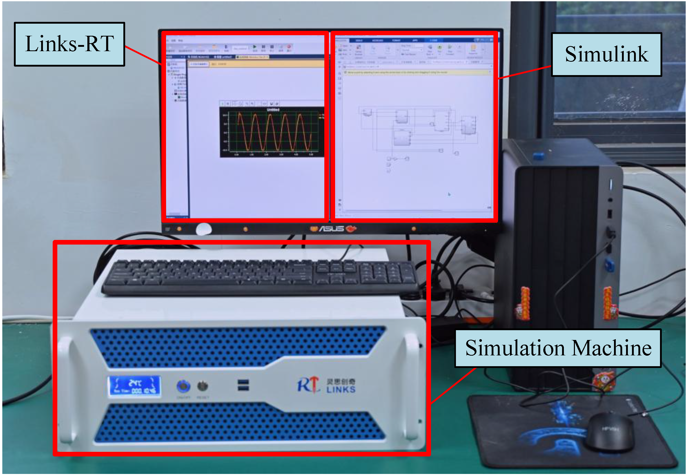
To validate the effectiveness of the proposed fixed-time sliding-mode control algorithm based on a piecewise approaching law, an experimental hardware-in-the-loop platform is implemented, as illustrated in Figure 3. In this platform, the real-time simulation machine executes the PMSM model with current-loop control and the connected load-side subsystem model, including the gearbox and the ball screw, with a sampling period of 100 $\mathsf{\mu }$s through Links-RT software. The proposed controller is implemented separately in MATLAB/Simulink R2023b with a sampling period of 10 ms.

Figure 3. Hardware-in-loop experiment platform.

The values of the EMA system parameters in (2)–(7) are summarized in Table 1, which are primarily adopted from the benchmark EMA model in [22]. Furthermore, the actual maximum speed during the experiments is approximately 1500 rpm, accounting for 50% of the rated value. The rated load-side torque of the adopted EMA model is 16.3 $\mathrm{N}·\mathrm{m}$, and its linear stroke is limited to 100 mm. Accordingly, the lumped disturbance torque $T_f$ is bounded by the rated torque, and the displacement command is constrained within the stroke range. It should be noted that although the numerical values adopted here differ from the EMA parameters of an actual aircraft, they are used solely to verify the effectiveness of the proposed control method.

Table 1. Parameters of the EMA system.

Name	Parameters	Value	Unit
Rotor inertia	$J_m$	$2.4\times {10}^{-4}$	$\mathrm{kg}·{\mathrm{m}}^2$
Motor damping coefficient	$B_m$	$0.01$	$\mathrm{N}·\mathrm{m}·\mathrm{s}/\mathrm{rad}$
Motor Torque constant	$K_t$	$0.16$	$\mathrm{N}·\mathrm{m}/\mathrm{A}$
Motor rated current	$I_N$	5	A
Motor rated speed	$n_N$	3000	rpm
Motor rated torque	$T_N$	$1.1$	$\mathrm{N}·\mathrm{m}$
Gear reduction ratio	n	15	−
Equivalent load inertia	$J_l$	$0.103$	$\mathrm{kg}·{\mathrm{m}}^2$
Equivalent viscous friction coefficient	$B_l$	$0.01$	$\mathrm{N}·\mathrm{m}·\mathrm{s}/\mathrm{rad}$
Concentrated torque stiffness	$K_l$	$1\times {10}^3$	$\mathrm{N}·\mathrm{m}/\mathrm{rad}$
Ball-screw lead	$P_h$	$0.005$	m

To achieve superior position control performance, the selection of control parameters in this work follows a multi-stage optimization strategy with the priority of ensuring system stability. First, the adjustable ranges of parameters are defined in accordance with the stability criteria derived from Lemma 1–3 to guarantee the asymptotic stability of the closed-loop system. Second, the sliding surface parameters of the motor-side and load-side subsystems are individually tuned under the ideal condition without external disturbances and the disturbance observer. This tuning process is based on the fixed-time convergence theory to optimize the tracking performance of the system in the disturbance-free scenario. Third, torque disturbances and the prescribed-time sliding-mode observer are introduced independently, the observer is configured with a prescribed convergence time and other sliding-mode parameters to ensure fast disturbance estimation while maximizing the smoothness of the observed values. Finally, the sliding-mode observer and the electrical/load-side sliding-mode controllers are integrated into the overall control system. The parameters of the three modules are co-optimized by comprehensively evaluating the rapidity of disturbance estimation, position-tracking performance, chattering amplitude of the inner and outer loops, and system robustness. The core of this co-optimization lies in improving the estimation performance of the sliding-mode observer to ensure the strong disturbance rejection capability of the system. The final optimized control parameters of the system are presented in Table 2.

Table 2. Controller parameters for the proposed method with piecewise approaching law.

Parameter	Value	Notes
Prescribed-time Observer
$\varpi$	0.5	Prescribed-time observer gain
$t_1$	0.2 s	Observation time constant
$t_2$	0.2 s	Additional time constant
$\Delta$	20	Disturbance bound or threshold
$s_q\left(0\right)$	0	Initial sliding variable value
Load-side Controller
${\alpha }_a$	0.88	Gain parameter
${\beta }_a$	1.12	Gain parameter
$k_1$	3.4	Controller gain
$k_2$	1.3	Controller gain
$c_1$	30	Gain parameter
$c_2$	25	Gain parameter
$c_3$	35	Gain parameter
$c_4$	20	Gain parameter
${\chi }_a$	1.65	Ratio/parameter
${\chi }_b$	0.6	Ratio/parameter
Motor-side Controller
${\alpha }_b$	0.87	Gain parameter
${\beta }_b$	1.13	Gain parameter
$k_3$	6.5	Controller gain
$k_4$	4.2	Controller gain
$c_5$	27	Gain parameter
$c_6$	19	Gain parameter
$c_7$	34	Gain parameter
$c_8$	26	Gain parameter
${\chi }_c$	1.4	Ratio/parameter
${\chi }_d$	0.65	Ratio/parameter

The proposed method is then compared with two baseline controllers. Method 1 is the conventional FxTSMC, while Method 2 is a PID controller adopted as a simplified baseline for performance comparison. The PID parameters are set to $K_p=0.075\mathrm{A}/\mathrm{mm}$, $K_i=0.9\mathrm{A}/(\mathrm{mm}·\mathrm{s})$ and $K_d=0.014\mathrm{A}·\mathrm{s}/\mathrm{mm}$, respectively, which are manually tuned based on the standard three-stage engineering procedure. First, $K_p$ is adjusted to ensure fast dynamic response and small error, yielding an approximate settling time of 1 s and a steady-state error of about 2 mm. Then, $K_i$ is introduced to eliminate steady-state error, but it exhibits weak damping characteristics with at least 40% overshoot and multi-peak oscillations. Therefore, $K_d$ is further tuned to suppress the oscillations induced by $K_i$, which cannot be adequately mitigated by $K_p$ and $K_i$ alone. In addition, the PID controller incorporates an anti-windup mechanism to avoid integral saturation.

4.1. Simulation Analysis of Disturbance Observation by the Prescribed-Time Integral Sliding-Mode Observer

The proposed prescribed-time integral sliding-mode observer is employed to accurately estimate the load-side disturbance torque of the EMA system. The target closed-loop position bandwidth of the EMA system is designed as 10 Hz, which meets the typical requirements of aerospace servo actuation systems.

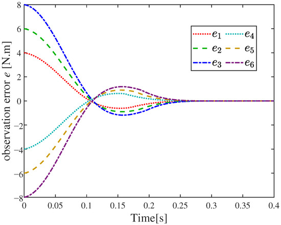
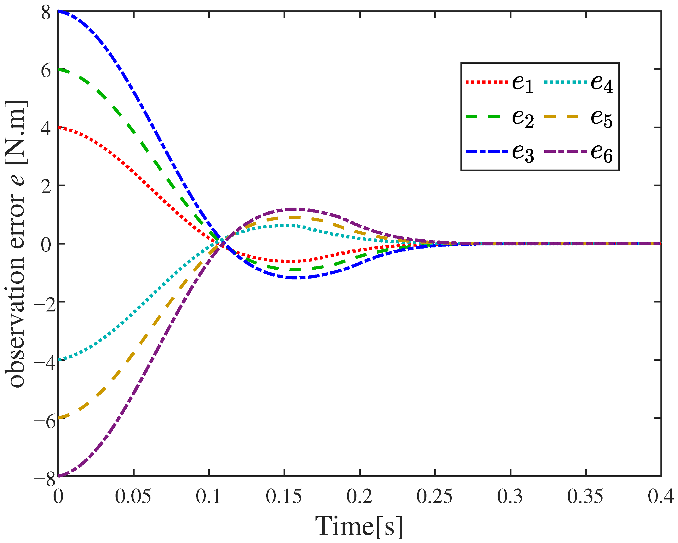
To validate the performance of the developed observer, while the system stably tracks a sinusoidal command with an amplitude of 60 mm and a frequency of 2 Hz, the estimation errors are evaluated under various external step torque disturbances of ±4 N·m, ±6 N·m and ±8 N·m, which account for 24.5%, 36.8% and 49.1% of the rated load-side torque (16.3 N·m), respectively. The corresponding results are illustrated in Figure 4.

Figure 4. Different torque disturbances observation error curves.

It can be seen that the error curves are plotted for the interval 0–$0.4$ s based on the proposed observer. A small overshoot occurs in the $0.1$–$0.3$ s range. The convergence time of the estimation error is approximately $0.3$ s, which is shorter than the theoretically computed conservative upper bound $T_o=t_1+t_2=0.4$ s. This validates the accuracy of the observer and the conservatism of the theoretical convergence bound. The presence of the prescribed-time observer enables rapid and precise disturbance estimation, providing fast feedforward compensation for the controller.

4.2. Simulation Analysis of Convergence for a Fixed-Time Sliding-Mode Controller

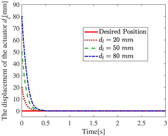
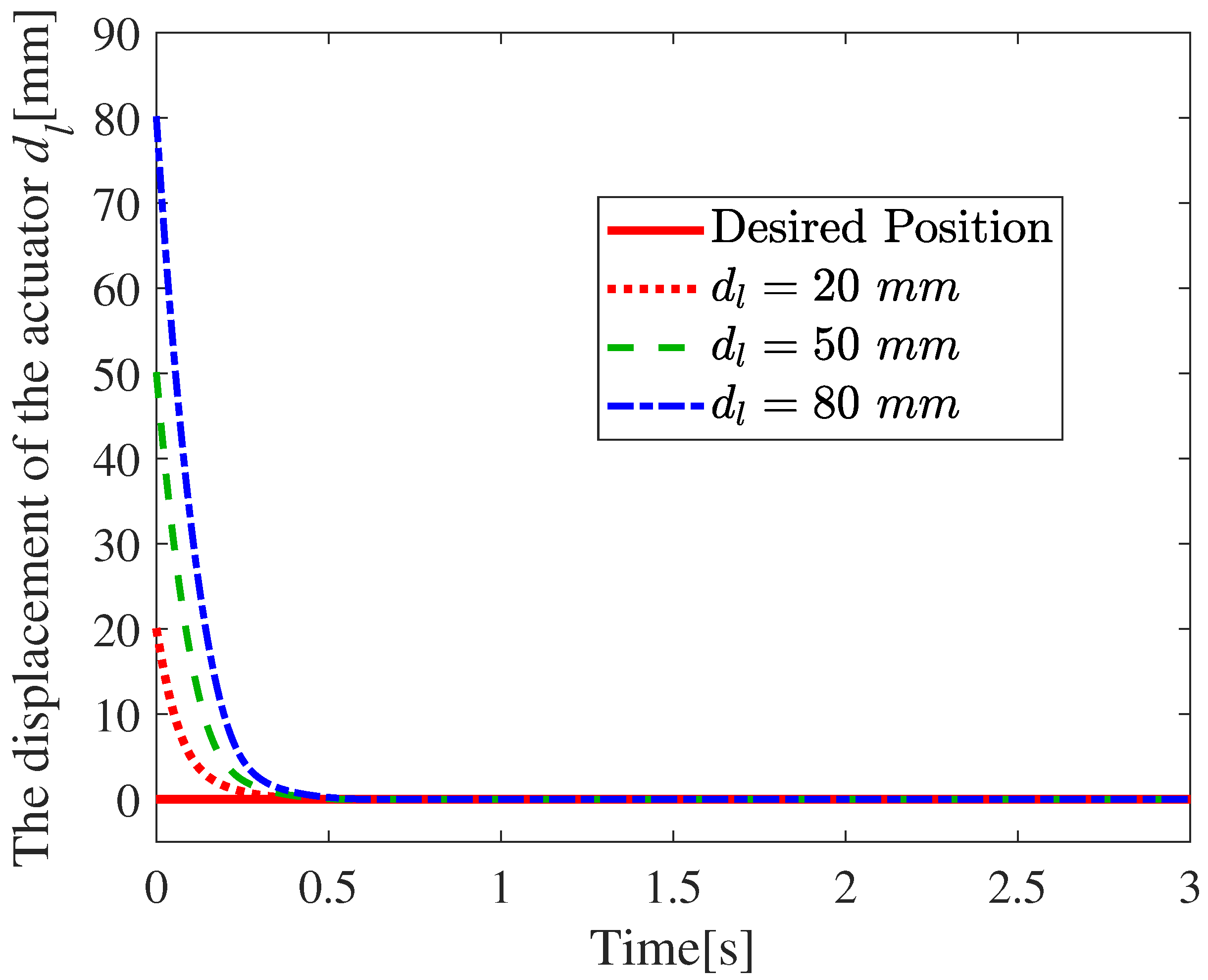
To validate the fixed-time convergence properties of the proposed controller, simulations were conducted under various desired displacement commands of 20 mm, 50 mm, and 80 mm, which are 20%, 50%, and 80% of the rated value. The corresponding tracking errors are depicted in Figure 5.

Figure 5. Fixed-time convergence of actuator displacement with initial distances.

As shown in Figure 5, for all admissible initial distances $d_l$, the system achieves stable convergence within $1.0$ s, with the trajectories exhibiting a rapid decay toward the target value and subsequently stabilizing. The theoretical fixed-time convergence upper bound for the load-side/motor-side control laws is derived from Section 3, which is independent of initial system conditions, verifying that the convergence speed of the proposed sliding-mode controller is uniquely determined by control parameters and possesses fixed-time convergence characteristics irrelevant to initial conditions. After convergence, the output remains in a near-zero radian steady-state region, indicating effective suppression of persistent disturbances and reliable fast steady-state tracking. The observed results are in good agreement with the theoretical analysis, further confirming the universality and practicality of the designed control law under varying initial conditions.

4.3. Displacement Step Tracking Results

To highlight the effectiveness of the fixed-time sliding-mode control based on the segmented reaching law, this section introduces step disturbance torque and sine disturbance torque at 3 s based on the 50 mm position step tracking. The position-tracking curve, the observation curve of the prescribed-time integral sliding-mode observer, and the convergence curve of the fixed-time controller are presented. Regarding the position-tracking curve graph, the traditional PID control and the traditional fixed-time sliding-mode control are provided as comparison benchmarks, which are briefly described as follows:

• Method 1: Traditional fixed-time sliding-mode control method.
• Method 2: PID control method.
• Proposed: The fixed-time sliding-mode control method based on the segmented reaching law.

4.3.1. Step Torque Disturbance Results

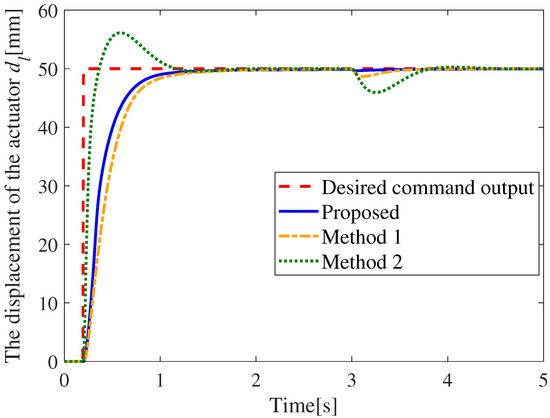
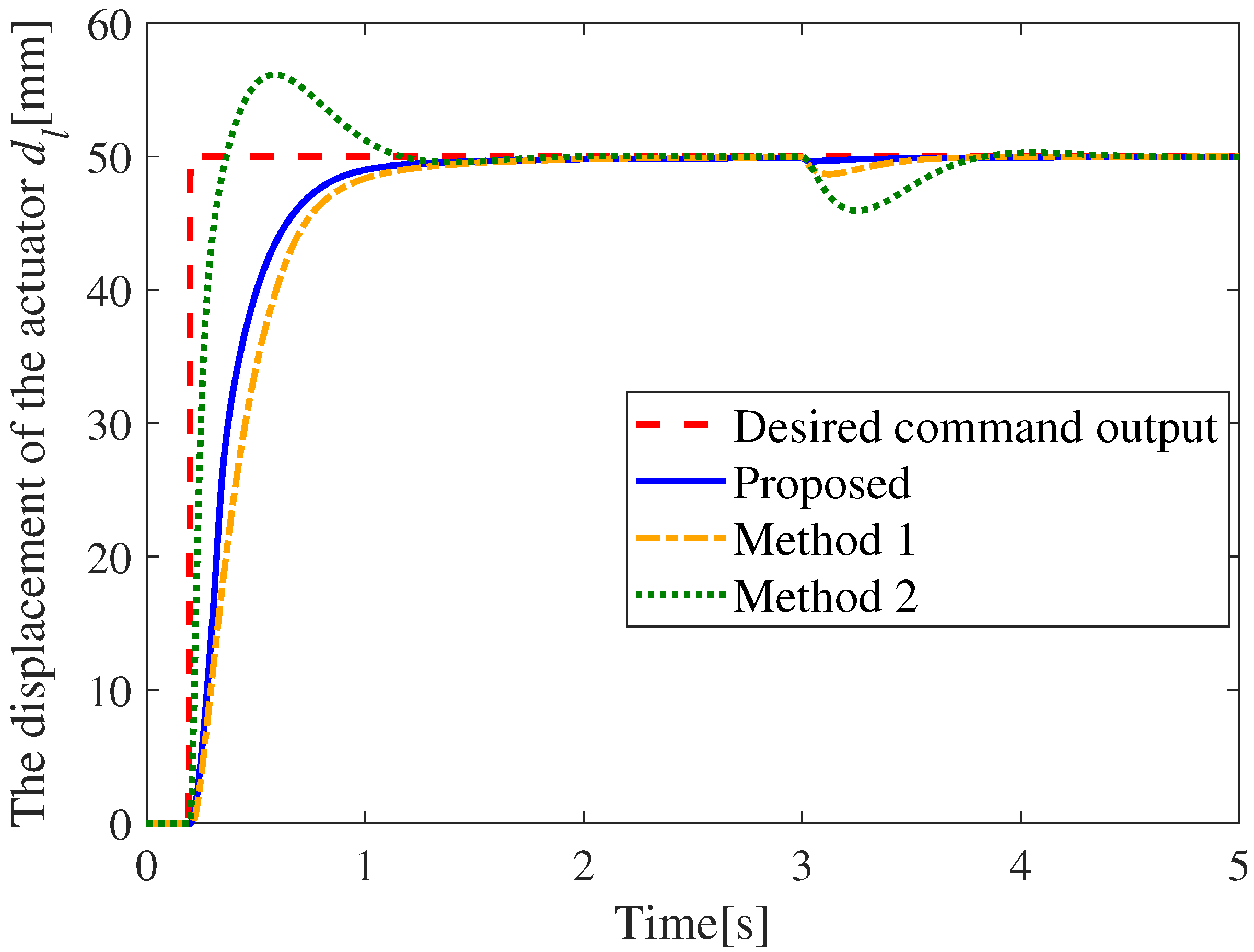
The step command tracking curves of the three algorithms are illustrated in Figure 6, where positive and negative torque disturbances of 10 N·m and $-6$ N·m are introduced at $t=3$ s, and the PID control is not equipped with a prescribed-time convergence observer.

Figure 6. Step response curve under step disturbance.

As illustrated in Figure 6, during the step response, the PID controller exhibits an overshoot of approximately 25%, whereas both the conventional FxTSMC and the proposed algorithm achieve zero overshoot, indicating superior transient stability. Evaluated under a ±5% tolerance band, the proposed algorithm yields a settling time of 0.58 s, outperforming the PID controller’s 0.71 s and the conventional FTSMC’s 0.61 s.

After a torque disturbance of 10 N·m is applied at $t=3\mathrm{s}$, the PID controller suffers a maximum transient drop of 8.14% and requires 0.71 s to recover within a 1% tolerance band. While the conventional FxTSMC limits the maximum drop(overshoot) to 2.6% and shortens the recovery time to 0.39 s, representing improvements of over 62.8% and 50.1% compared to the PID controller, respectively. More remarkably, subject to the same torque disturbance, the peak output deviation of the proposed algorithm is restricted to only 0.35 mm, which is less than 0.71% of the steady-state value. This equates to a reduction in peak deviation of over 94.3% and 84.3% compared to the PID controller and the conventional FxTSMC, respectively. Furthermore, the proposed algorithm restores the system to the steady state within merely 0.11 s. Compared to the PID controller and the conventional FxTSMC, the recovery time is reduced by 80.7% and 60.7%, respectively, thoroughly substantiating the excellent convergence and strong robustness of the proposed strategy.

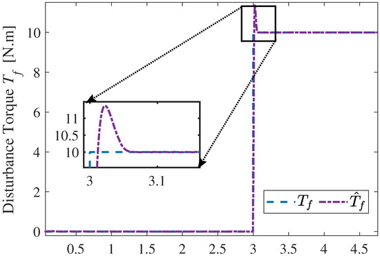
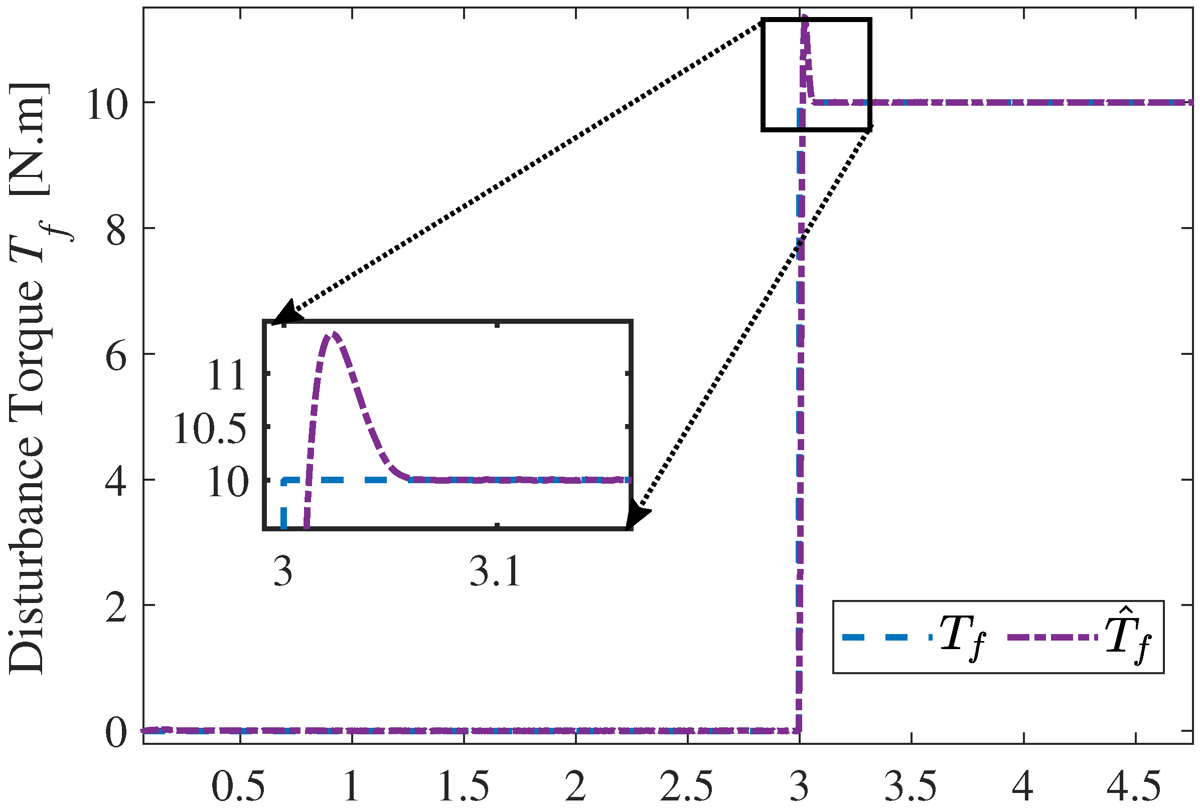
The observation curve of the proposed observer for the torque disturbance is illustrated in Figure 7.

Figure 7. Results of the proposed observer with positive step disturbance under the step command.

It can be seen that when the positive torque changes abruptly, the output of the observer shows an overshoot of 13.68%, but the adjustment time of 0.07 s is much shorter than the theoretically prescribed convergence time $T_o=0.4$ s, which allows the observer to track the changes in torque quickly, providing high-response disturbance information support for the feedforward compensation link of the control system.

4.3.2. Sinusoidal Torque Disturbance Results

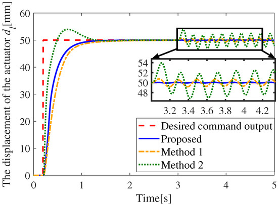
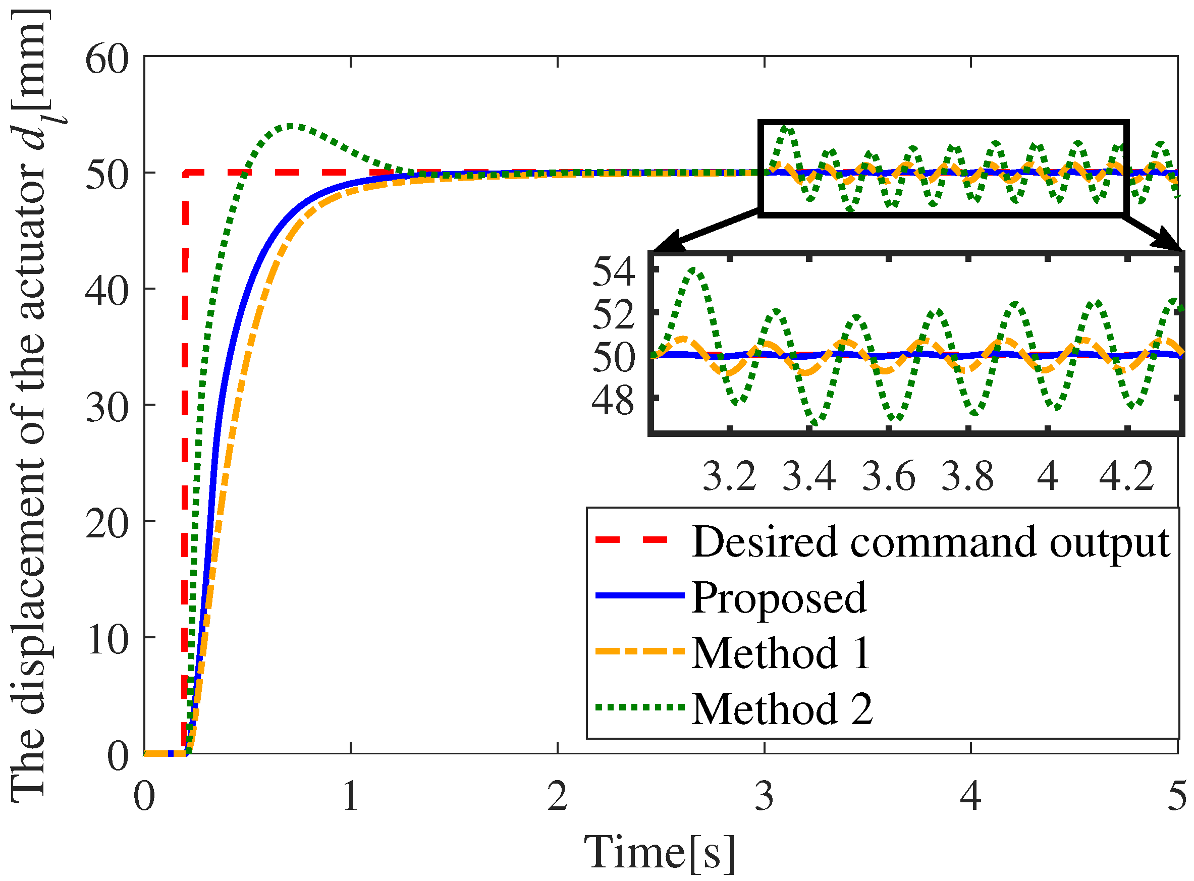
Figure 8 presents the response curves of the three algorithms under step command tracking, with a sinusoidal torque disturbance introduced at t = 3 s. From the curves, it can be observed that, under the application of sinusoidal disturbance, the PID method exhibits sinusoidal displacement fluctuations of ±4% relative to the steady-state value. The traditional FxTSMC shows a sinusoidal fluctuation of 0.46%, which is a 88.5% reduction in displacement fluctuation compared with the PID method. In comparison, the proposed method does not exceed 0.02% of the steady-state value, indicating that its anti-disturbance performance is far superior to that of the PID algorithm and the traditional FxTSMC algorithm.

Figure 8. Step response under sine disturbance.

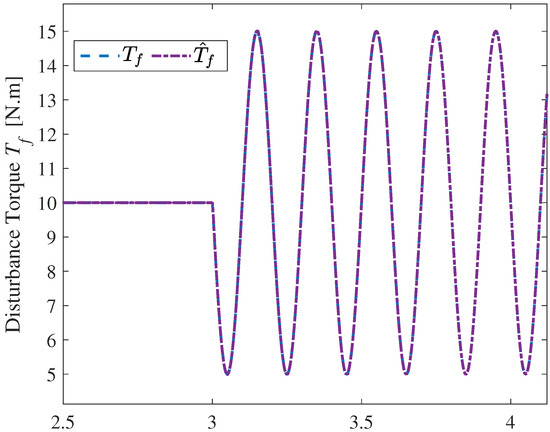
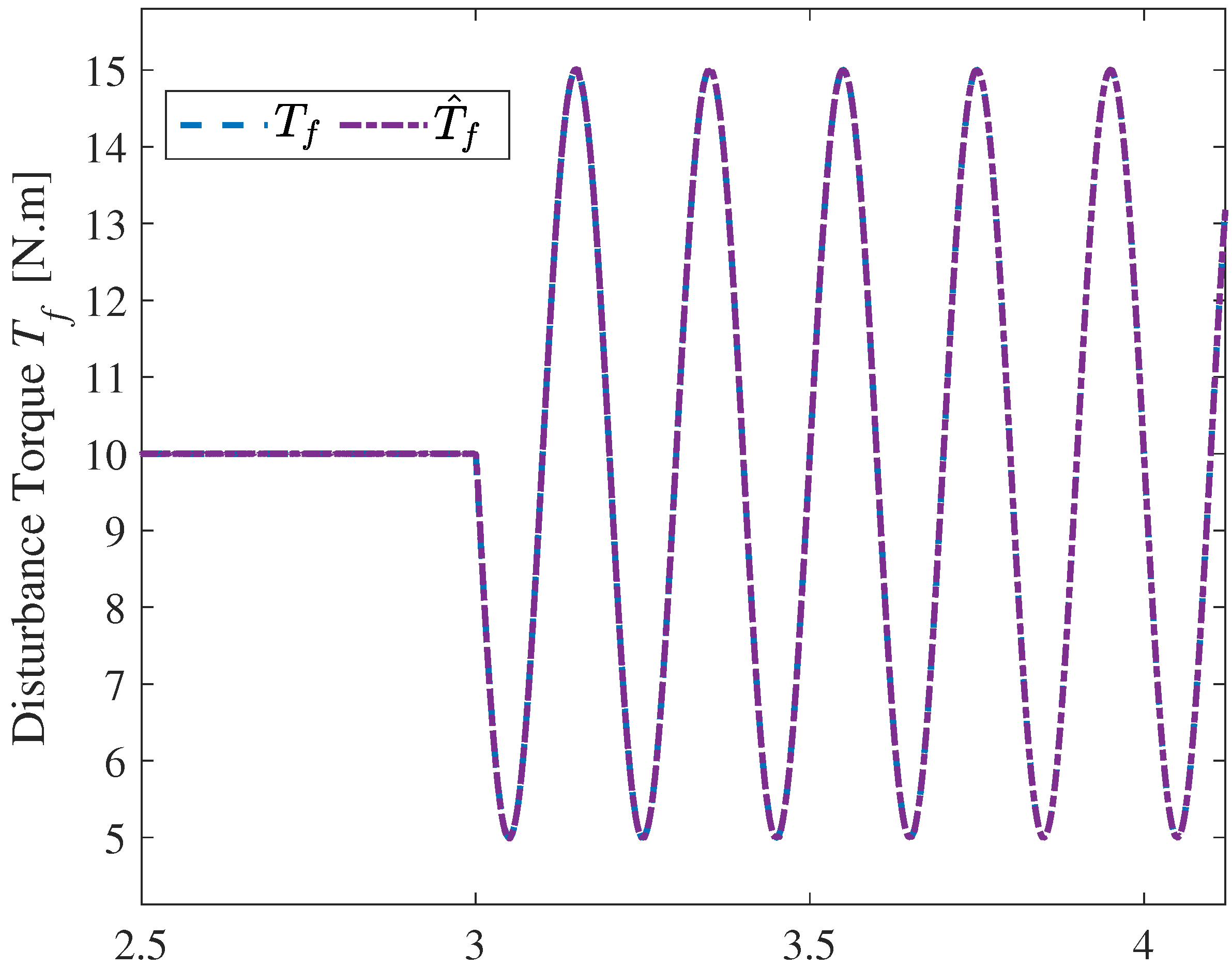
Figure 9 shows the result of the prescribed-time observer for this sinusoidal torque disturbance. It can be seen that after the sinusoidal disturbance is introduced at t = 3 s, although the estimated torque output by the observer has a brief dynamic deviation in the initial stage, it can quickly track the sinusoidal variation law of the actual disturbance. The adjustment process has a fast response speed and high observation accuracy, providing reliable disturbance information support for the feedforward compensation of the control system.

Figure 9. Results of the proposed observer with sinusoidal disturbance under the step command.

4.4. Displacement Sine Curve Tracking Results

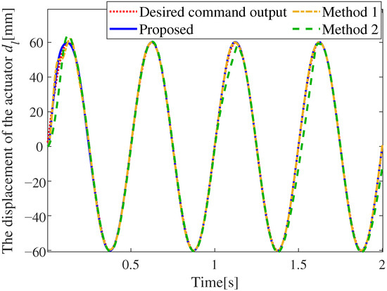
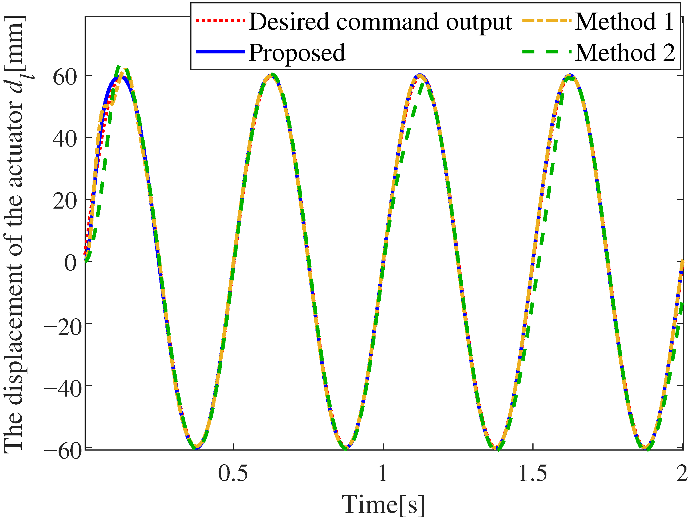
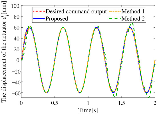
To verify the control performance of the proposed algorithm in the dynamic signal tracking scenario, the amplitude of the sinusoidal command signal was set to 60 mm with a frequency of 2 Hz, and simulations were carried out under the conditions of step disturbance torque and sinusoidal disturbance torque respectively.

4.4.1. Constant Torque Disturbance Results

Figure 10 illustrates the dynamic response of the three algorithms during sinusoidal command tracking, where a torque disturbance is introduced at $t=1$ s. The performance of the observer in this scenario is consistent with that presented in Figure 4, except that the disturbance application time is set to $t=1$ s. Before the occurrence of the torque disturbance, the PID controller exhibits a maximum tracking error of $21.24\mathrm{mm}$ at $t=0.054\mathrm{s}$. The conventional FxTSMC restricts the maximum tracking error to $8.51\mathrm{mm}$ at $t=0.048\mathrm{s}$. In stark contrast, the proposed algorithm significantly reduces the maximum tracking error to $4.51\mathrm{mm}$ at $t=0.011\mathrm{s}$. Upon the introduction of the step torque disturbance at $t=1\mathrm{s}$, the PID controller suffers severe transient degradation, with the maximum tracking error surging to $10.85\mathrm{mm}$. Conversely, both the conventional FxTSMC and the proposed algorithm exhibit comparable, robust disturbance rejection capabilities, tightly limiting the maximum error deviation to merely $1.19\mathrm{mm}$. Overall, while both SMC-based methods demonstrate excellent robustness against external disturbances, the proposed algorithm distinctly outperforms the alternatives in terms of dynamic tracking precision.

Figure 10. Sine response under step disturbance.

4.4.2. Sine Torque Disturbance Results

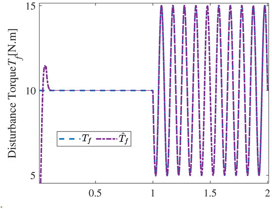
To further evaluate the system’s resilience against time-varying uncertainties during dynamic command tracking, a continuous sinusoidal disturbance is introduced at $t=1\mathrm{s}$. The response of the three algorithms during sinusoidal command tracking is illustrated in Figure 11 and the performance of the observer is illustrated in Figure 12.

Figure 11. Sine response under sine disturbance.

Figure 12. Results of the proposed observer with sinusoidal disturbance under the sinusoidal command.

The PID controller suffers a severe degradation in tracking precision subjected to this disturbance, which exhibits a substantial peak tracking error of $6.12\mathrm{mm}$. The conventional FxTSMC achieves more satisfactory tracking fidelity, containing the maximum negative tracking error to $1.24\mathrm{mm}$. Remarkably, the proposed algorithm demonstrates markedly superior robustness against such continuous, time-varying disturbances. Its tracking error is tightly constrained to within $0.27\mathrm{mm}$, yielding an improvement of over 78.3% compared to the traditional FxTSMC. These results comprehensively validate the exceptional dynamic convergence and robust disturbance rejection properties of the proposed approach.

4.4.3. High Frequency Sine Command Tracking Performance of the Proposed Controller

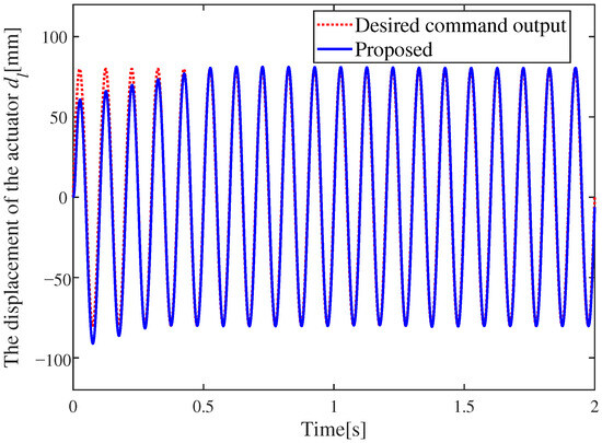
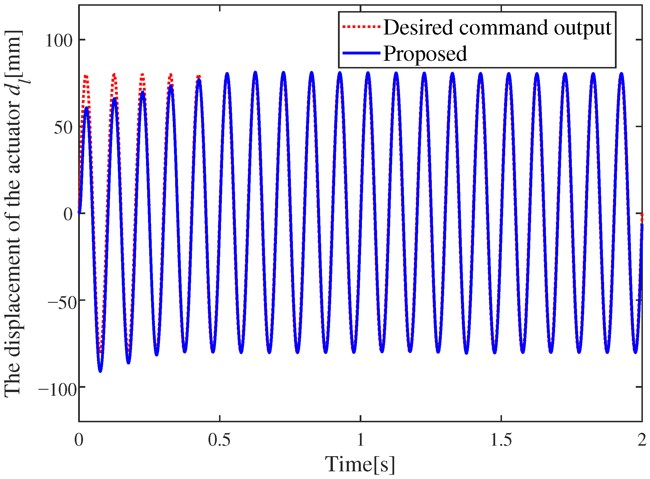
To validate the tracking capability of the proposed controller under a high-frequency command signal, a sinusoidal reference with a frequency of 10 Hz and an amplitude of 80 mm was considered. The corresponding tracking result is presented in Figure 13.

Figure 13. The displacement of the actuator under a 10 Hz sinusoidal curve with 80 mm amplitude.

It can be observed that, although the tracking performance is unsatisfactory during the initial transient stage, the tracking error gradually decreases after 0.3 s of adjustment, which verifies that the proposed controller still possesses good tracking capability under the high frequency operating condition of 10 Hz.

4.5. Robustness Analysis Against Parameter Perturbation

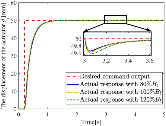
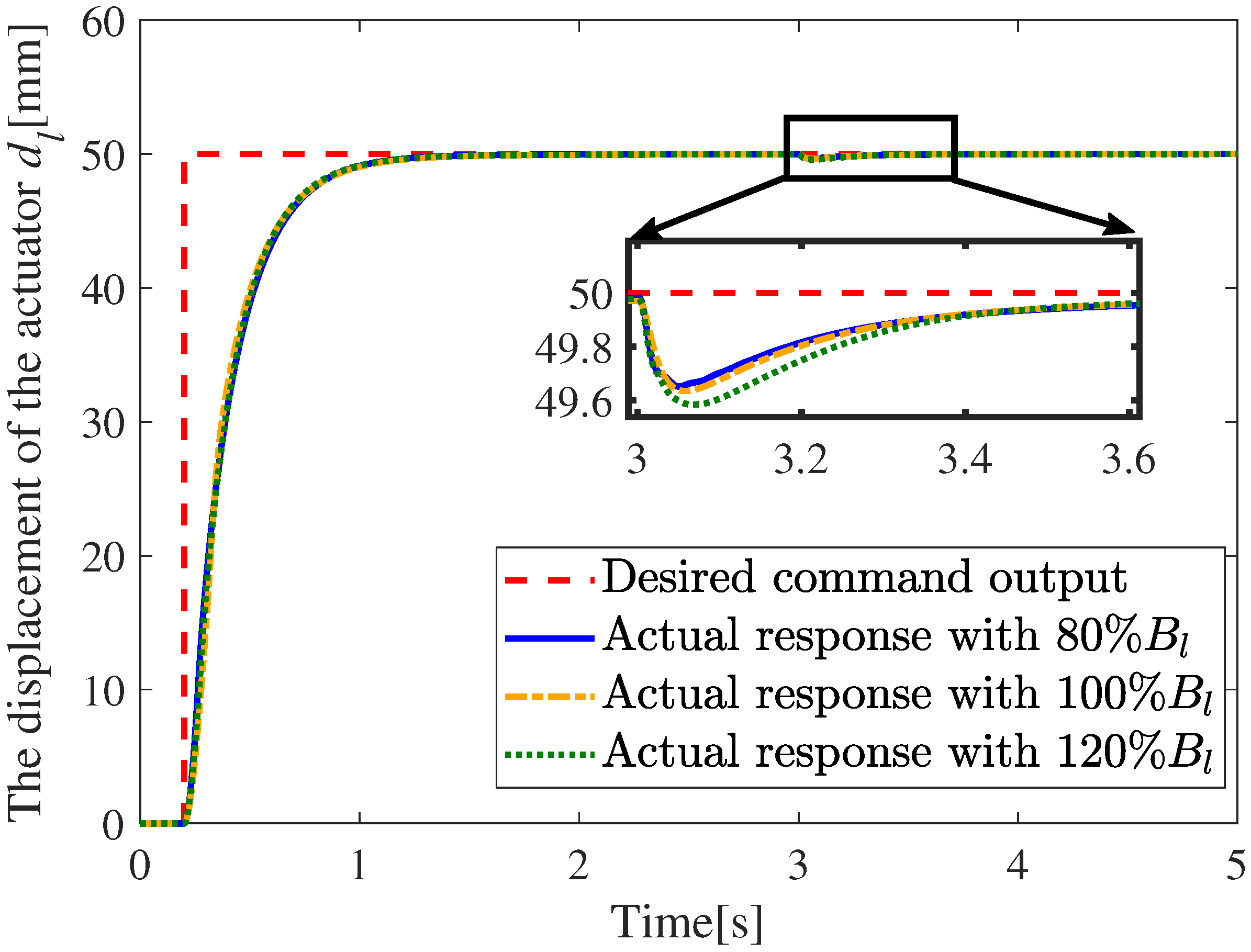
To verify the robustness of the proposed fixed-time sliding-mode control algorithm against parameter perturbation or modeling uncertainties, the step response performance of the system is tested under different viscous friction coefficient $B_l$ conditions, and the results are shown in Figure 14.

Figure 14. Step response of the EMA system under different $B_l$ parameter perturbations, verifying the strong robustness of the proposed control algorithm.

It can be observed from the figure that when $B_l$ is perturbed to 80%, 100% and 120% of the nominal value, the actual displacement response of the actuator can still track the desired command output accurately and rapidly. The convergence time of the system is basically unaffected by the above parameter perturbations, and all responses can reach the steady-state value rapidly. Even in the local enlarged view of the steady-state stage, the three curves under different parameter perturbations only present extremely small differences, and all can quickly converge to the desired value with almost no steady-state error. This fully demonstrates that the proposed control algorithm has strong robustness to the parameter perturbation of $B_l$, and the parameter variation has negligible influence on both the dynamic response and control performance of the system, which can ensure the stable and reliable operation of the EMA system under uncertain working conditions.

5. Conclusions

To address the challenge of mismatched external disturbances in electromechanical actuator systems, this paper proposes a position-tracking strategy that integrates a fixed-time sliding-mode scheme within a backstepping control framework. A prescribed-time integral sliding-mode observer is implemented to estimate unmeasurable load disturbances, with its convergence time strictly pre-calculated and guaranteed via Lyapunov stability theory. Furthermore, a piecewise reaching law is designed to construct the fixed-time controller, which effectively mitigates the chattering phenomenon while ensuring that system convergence remains independent of initial states. The proposed control framework achieves effective disturbance compensation and demonstrates faster transient response and superior tracking accuracy compared to PID and traditional FxTSMC algorithm. Specifically, under step disturbances, the peak deviation in step response is only 0.25% of the steady-state value, reduced by 94.2% and 84.3% compared with PID and traditional FxTSMC, respectively, and the recovery time is shortened by 80.7% and 60.7%. Under sinusoidal disturbances, the output fluctuation remains below 0.02% of the steady-state value, outperforming traditional FxTSMC with 0.46%. In the scenario of sinusoidal tracking with an added step disturbance, the maximum tracking error is 1.19 mm which is superior to the PID controller’s error of 10.85 mm. Moreover, under a sinusoidal disturbance, the maximum error is confined to within 0.27 mm, less than both PID and conventional FxTSMC.

References

- Fu, J.; Maré, J.C.; Fu, Y. Modelling and simulation of flight control electromechanical actuators with special focus on model architecting, multidisciplinary effects and power flows. Chin. J. Aeronaut. 2017, 30, 47–65. [Google Scholar] [CrossRef] [Scilit]
- Annaz, F.Y.; Kaluarachchi, M.M. Progress in Redundant Electromechanical Actuators for Aerospace Applications. Aerospace 2023, 10, 787. [Google Scholar] [CrossRef] [Scilit]
- Rosero, J.; Ortega, J.; Aldabas, E.; Romeral, L. Moving towards a more electric aircraft. IEEE Aerosp. Electron. Syst. Mag. 2007, 22, 3–9. [Google Scholar] [CrossRef] [Scilit]
- Giangrande, P.; Madonna, V.; Sala, G.; Kladas, A.; Gerada, C.; Galea, M. Design and Testing of PMSM for Aerospace EMA Applications. In Proceedings of the IECON 2018—44th Annual Conference of the IEEE Industrial Electronics Society, Washington, DC, USA, 21–23 October 2018; pp. 2038–2043. [Google Scholar]
- Fang, Q.; Zhou, Y.; Ma, S.; Zhang, C.; Wang, Y.; Huangfu, H. Electromechanical Actuator Servo Control Technology Based on Active Disturbance Rejection Control. Electronics 2023, 12, 1934. [Google Scholar] [CrossRef] [Scilit]
- Liu, C.; Luo, G.; Duan, X.; Chen, Z.; Zhang, Z.; Qiu, C. Adaptive LADRC-Based Disturbance Rejection Method for Electromechanical Servo System. IEEE Trans. Ind. Appl. 2020, 56, 876–889. [Google Scholar] [CrossRef]
- Liu, C.; Luo, G.; Chen, Z.; Tu, W. Finite-Time Convergent Multiple Disturbance Rejection Control for Electromechanical Actuators. IEEE Trans. Power Electron. 2021, 36, 6863–6878. [Google Scholar] [CrossRef] [Scilit]
- Zuo, Q.; Wang, B.; Chen, J.; Dong, H. Model Predictive Control of Aero-Mechanical Actuators with Consideration of Gear Backlash and Friction Compensation. Electronics 2024, 13, 4021. [Google Scholar] [CrossRef] [Scilit]
- Yuan, S.; Deng, W.; Yi, W.; Yao, J.; Yang, G.; Guan, J. Adaptive Robust Stable Tracking Control of Two-Axis Coupled Electromechanical Actuation System Based on Friction Compensation. Actuators 2025, 14, 396. [Google Scholar] [CrossRef] [Scilit]
- Todić, I.; Miloš, M.; Pavišić, M.N. Position and speed control of electromechanical actuator for aerospace applications. Teh. Vjesn. 2013, 20, 853–860. [Google Scholar]
- Xiao, X.; Xiong, S.; Wu, X.; Liu, D. Research on improved control method of electromechanical actuation. J. Eng. 2018, 2018, 631–635. [Google Scholar] [CrossRef] [Scilit]
- Liu, C.; Luo, G.; Chen, Z.; Tu, W.; Qiu, C. A linear ADRC-based robust high-dynamic double-loop servo system for aircraft electro-mechanical actuators. Chin. J. Aeronaut. 2019, 32, 2174–2187. [Google Scholar] [CrossRef] [Scilit]
- Nguyen, T.T.; Tran, H.N.; Nguyen, T.H.; Jeon, J.W. Recurrent Neural Network-Based Robust Adaptive Model Predictive Speed Control for PMSM With Parameter Mismatch. IEEE Trans. Ind. Electron. 2023, 70, 6219–6228. [Google Scholar] [CrossRef] [Scilit]
- Cao, H.; Deng, Y.; Zuo, Y.; Liu, X.; Wang, J.; Lee, C.H.T. A Variable Structure ADRC for Enhanced Disturbance Rejection and Improved Noise Suppression of PMSM Speed System. IEEE Trans. Ind. Electron. 2025, 72, 4481–4495. [Google Scholar] [CrossRef] [Scilit]
- Ding, S.; Hou, Q.; Wang, H. Disturbance-Observer-Based Second-Order Sliding Mode Controller for Speed Control of PMSM Drives. IEEE Trans. Energy Convers. 2023, 38, 100–110. [Google Scholar] [CrossRef] [Scilit]
- Wang, Q.; Yu, H.; Wang, M.; Qi, X. An Improved Sliding Mode Control Using Disturbance Torque Observer for Permanent Magnet Synchronous Motor. IEEE Access 2019, 7, 36691–36701. [Google Scholar] [CrossRef] [Scilit]
- Zhang, L.; Tao, R.; Zhang, Z.X.; Chien, Y.R.; Bai, J. PMSM non-singular fast terminal sliding mode control with disturbance compensation. Inf. Sci. 2023, 642, 119040. [Google Scholar] [CrossRef] [Scilit]
- Lin, X.; Wu, C.; Yao, W.; Liu, Z.; Shen, X.; Xu, R.; Sun, G.; Liu, J. Observer-Based Fixed-Time Control for Permanent-Magnet Synchronous Motors With Parameter Uncertainties. IEEE Trans. Power Electron. 2023, 38, 4335–4344. [Google Scholar] [CrossRef] [Scilit]
- Trinh, H.M.; Nguyen, T.H.; Nguyen, T.T.; Jeon, J.W. Robust Adaptive Learning Rate Neural Network State Observer Based Fixed-Time Sliding Mode Control of a Permanent Magnet Synchronous Motor. IEEE Trans. Power Electron. 2026, 41, 1826–1840. [Google Scholar] [CrossRef] [Scilit]
- Jahns, T.M.; Kliman, G.B.; Neumann, T.W. Interior Permanent-Magnet Synchronous Motors for Adjustable-Speed Drives. IEEE Trans. Ind. Appl. 1986, IA-22, 738–747. [Google Scholar] [CrossRef] [Scilit]
- Shi, Z.; Zhang, P.; Lin, J.; Ding, H. Permanent Magnet Synchronous Motor Speed Control Based on Improved Active Disturbance Rejection Control. Actuators 2021, 10, 147. [Google Scholar] [CrossRef] [Scilit]
- Sun, H.; Jiang, J.; Xiao, X. Fuzzy Active Disturbance Rejection Control for Electro-Mechanical Actuator Based on Feedback Linearization. Actuators 2026, 15, 18. [Google Scholar] [CrossRef] [Scilit]
- Chen, C.; Li, L.; Peng, H.; Yang, Y.; Mi, L.; Wang, L. A new fixed-time stability theorem and its application to the synchronization control of memristive neural networks. Neurocomputing 2019, 349, 290–300. [Google Scholar] [CrossRef] [Scilit]
- Cui, L.; Jin, N.; Chang, S.; Zuo, Z.; Zhao, Z. Fixed-time ESO based fixed-time integral terminal sliding mode controller design for a missile. ISA Trans. 2022, 125, 237–251. [Google Scholar] [CrossRef] [Scilit]
Disclaimer/Publisher’s Note: The statements, opinions and data contained in all publications are solely those of the individual author(s) and contributor(s) and not of MDPI and/or the editor(s). MDPI and/or the editor(s) disclaim responsibility for any injury to people or property resulting from any ideas, methods, instructions or products referred to in the content. |
© 2026 by the authors. Licensee MDPI, Basel, Switzerland. This article is an open access article distributed under the terms and conditions of the Creative Commons Attribution (CC BY) license.