


Abstract
This paper explores the emerging synergy between control theory and machine learning in robotics, focusing on methods that combine model-based strategies with data-driven adaptation. The authors highlight how classical techniques, such as model predictive control and adaptive control, are being enhanced by reinforcement learning, imitation learning, and neural models to address challenges in complex, uncertain environments. Emphasis is placed on real-world platforms (e.g., legged systems, aerial robots, and manipulators) with special attention to advanced domains such as multi-agent systems and coordination. The authors, in addition, establish a taxonomy to categorize these hybrid approaches as “learning-for-control”, “control-for-learning”, or “co-designed architectures”. This paper also reflects upon key open problems, including sim-to-real transfer, safety, and the need for verifiable learning-based controllers, all facets that help to outline a roadmap for future research.
1. Introduction
The field of robotics is in the midst of a profound transformation. Traditionally confined to structured, predictable environments such as automotive assembly lines, robots are rapidly moving into the complex, dynamic, and uncertain spaces of human life. This shift is fueling a surge in diverse applications, from autonomous vehicles navigating densely populated, dynamically constrained urban environments [1], legged robots traversing unstructured terrain [2,3], agile aerial systems navigating in complex environments [4], and dexterous manipulators interacting with the physical world [5,6].
This grand challenge of achieving robust autonomy in real-world operating environments has highlighted a fundamental tension between two historically separate fields of research: classical control theory and modern machine learning.
For decades, the foundation of robotics has been focused within classical control theory, a discipline largely rooted in the work of mechanical and electrical engineering researchers. This approach leverages rigorous methods based on models such as Model Predictive Control (MPC) [7] and Adaptive Control [8], and more recently, Control Barrier Functions (CBFs) [9]. These tools are designed to provide stability, optimize performance, and, most importantly, offer proven guarantees of safety and behavior, which is required for safety-critical systems. However, the power of this approach hinges on the critical (and often unattainable) requirement of an accurate mathematical model of the robot and its environment. When the real-world environment inevitably deviates from this model (e.g., due to unmodeled friction, sudden disturbances, or complex contact physics), control performance can degrade rapidly.
The “AI explosion” of the last decade, driven by the computer science community, has introduced a radically different paradigm: Machine Learning (ML) driven by data. The advent of Deep Learning (DL) [10] and the maturation of Reinforcement Learning (RL) [11] and Imitation Learning (IL) [12,13] have provided tools that excel in facets where classical control falters. These ML methods can learn highly complex, nonlinear policies directly from data, often without any explicit a priori model. Seminal works have shown that deep neural networks can learn control policies directly from raw sensory inputs, achieving unprecedented performance on tasks previously thought to be intractably complex [5]. Yet, this power comes at a cost: a “black box” nature, a high demand for data, and a fundamental lack of formal guarantees. As such, the implementation of such techniques poses risks when deploying robots in scenarios critical for safety.
This paper is motivated by the fact that the state-of-the art is no longer defined by one of these pillars (i.e., control theory or ML), but by the synergy between them. The most significant breakthroughs in robotics today emerge from this fusion of rigor from models and flexibility from data. For instance, the precision of MPC is being enhanced by neural networks that learn complex dynamics, as demonstrated by methods such as Probabilistic Ensembles with Trajectory Sampling (PETS) [14], a concept further reviewed by Zhang et al. [15]. Conversely, the exploratory nature of RL is being made safe for physical hardware by using CBFs as a safety shield [16], a key topic within the broader field of safe learning [17]. At the deepest level of integration, optimization layers from control are being embedded directly into neural networks as differentiable components [18], creating structured policies that can be trained directly from raw sensory inputs. This hybrid approach promises the “best of both worlds”: controllers that use learning to adapt to model uncertainty while being supervised by control theoretic safety guarantees.
However, this convergence has also created a critical need. The rapid proliferation of hybrid methods has made it difficult to navigate the landscape. Control engineers may be unfamiliar with the nuances of learning algorithms, while computer scientists may not be well-versed in, for example, robust control. In this article, the authors focus on the confluence of control theory and machine learning and conduct a literature review on the latest advances of leveraging both control theory and machine learning to empower robotic applications, as illustrated in Figure 1.
Figure 1.
An illustration of control theory- and machine learning-enabled robotic applications: “Map of Control Theory” (top [19]), “Main types of machine learning” (middle [20]), and example robotic applications (bottom).
The authors provide a survey and taxonomy intended for a multidisciplinary audience. The goal is to synthesize the foundational concepts of both areas, categorize the diverse integration strategies, and provide a roadmap to understand and contribute to this emerging multidisciplinary field.
This paper is structured as follows: Section 2 reviews the foundational concepts from both control theory and machine learning. Section 3 surveys applications of these methods on real-world robotic platforms. Section 4 provides an overview into the advanced topic of Multi-Agent Reinforcement Learning. Section 5 introduces a novel taxonomy that categorizes integration strategies. Section 6 discusses key open problems and future directions, including safety and sim-to-real transfer. Section 7 concludes the review.
2. Foundational Concepts
This section reviews the foundational concepts from both control theory and machine learning that serve as the building blocks for modern robotics. The aim is to provide an overview of the mathematical formulations and structural paradigms that are more frequently combined and to show contrast between the model-based, guarantee-centric nature of classical control and that of the data-driven, flexible paradigms of machine learning.
2.1. Foundations in Control Theory
Classical control theory provides the tools for rigorous analysis, optimization, and safety. It is typically built upon an explicit mathematical model of system dynamics, generally denoted as , where represents the system state and is the control input. In general, controllers assume full state feedback (i.e., measurement) or that an observer is applied to estimate unmeasured states. The authors note that Model Predictive Control, Adaptive Control and Safety-Critical Control are used as example control techniques (without loss of generality).
2.1.1. Model Predictive Control (MPC)
Model Predictive Control (MPC) is a powerful and wildly-used framework for optimal control that operates on a receding horizon principle. Unlike simple feedback laws that react only to current errors, MPC anticipates future events.
The core mechanism is illustrated in Figure 2. At each sampling instant , MPC measures the current state and solves a constrained Finite-Horizon Optimal Control Problem (FHOCP). This optimization predicts a sequence of optimal control inputs over a horizon N to minimize a cost function while satisfying physical constraints. Of note, only the first input in this sequence is applied to the robotic platform. At the next time step , the state is measured again and the entire optimization is repeated. This “closed-loop” re-planning allows MPC to naturally take into account disturbances and modeling errors.
Figure 2.
Schematic of a standard Model Predictive Controler (MPC) with receding constrained horizon optimization ([21]).
The general mathematical formulation seeks to minimize a cost function J subject to the following dynamics and constraints:
where is the stage cost (often representing energy consumption or tracking error), is the terminal cost ensuring stability, and represent the feasible state and input sets (e.g., manipulator joint limits or actuator saturation).
- Linear vs. Nonlinear MPC
The level of complexity of this optimization problem (and, hence, the computation of the real-time solution thereof) depends heavily on the model . Linear MPC (LMPC) relies on linearized dynamics of the form . If the cost function is quadratic, the FHOCP reduces to a convex Quadratic Program (QP). Because QPs can be solved efficiently using active-set or interior-point methods [22,23], LMPC is highly effective for high-speed systems (e.g., quadrotors) that require high update rates.
In contrast, Nonlinear MPC (NMPC) directly utilizes the system’s full nonlinear dynamics . This is essential for robots with complex kinematics or non-holonomic constraints but results in a non-convex Non-Linear Programming (NLP) problem, which requires iterative solvers, such as Sequential Quadratic Programming (SQP) [22,24], and is computationally demanding [25].
- Explicit Model Predictive Control (eMPC)
For systems with fast dynamics where online optimization is computationally prohibitive, explicit MPC (eMPC) offers a solution by shifting the computational burden to offline processing. By treating the state vector as a parameter vector, the MPC problem can be reformulated as a Multi-Parametric Quadratic Program (mp-QP). The solution to this problem maps the state space partitioning into polyhedral critical regions . Within each region, the optimal control law is an explicit affine function of the state such that
where is the optimal gain matrix and is the offset vector associated with the i-th polyhedral region. This allows the online controller to be reduced to a simple point-location lookup table, drastically reducing processing. Recent works have demonstrated the efficacy of eMPC for real-time flight control of quadrotors with unbalanced payloads [26] and tracking control for Autonomous Surface Vehicles (ASVs) [27].
- Robust MPC
Standard MPC assumes that the model is perfect. However, real-world dynamics often include a disturbance vector , such that . To address this, Tube-based MPC constructs a “tube” of admissible trajectories about a nominal reference. An admissible trajectory represents a computed sequence of future states and control inputs that strictly satisfies all physical actuation limits and system constraints, while continuously guaranteeing mathematical stability under the worst case bounded disturbances projected over the entire prediction horizon. The control law, given as , consists of both a feedforward control for the nominal system and a feedback term , where is a local feedback gain matrix. This feedback controller addresses disturbances to maintain the state inside a bounded invariant set (i.e., the “tube”) centered about the nominal state [28].
2.1.2. Adaptive Control
While MPC takes into account disturbances via robustness margins, Adaptive Control is specifically designed to address parametric and time-varying uncertainty. In many robotic applications, the dynamic structure is known (e.g., as in rigid body dynamics), but specific parameters (e.g., payload mass, friction coefficients, or inertia tensors) are either unknown and/or vary over time.
For robotic manipulators, the Lagrangian dynamics are governed by the equation
where is the vector of joint positions, is the mass/inertia matrix, is the Centripetal and Coriolis matrix, is the gravity vector, and is the vector of generalized joint torques.
A key property utilized in adaptive control is that these dynamics can be linearly parameterized with respect to the unknown physical parameters (e.g., mass and inertia). This allows the dynamics to be rewritten as
where is the known kinematic regressor matrix and is the parameter vector to be estimated.
- Model Reference Adaptive Control (MRAC)
A canonical approach to adaptive control is Model Reference Adaptive Control, which is visualized in Figure 3. The core idea is to define a “Reference Model”, an ideal theoretical system , that exhibits a desired performance. In this formulation:
Figure 3.
Classical adaptive control system (picture courtesy of [29]).
- is the reference state vector.
- is the stable Hurwitz matrix defining the desired system dynamics.
- is the reference input matrix.
- is the reference command (e.g., the target trajectory or setpoint).
To address the inherent discrepancy between the nonlinear plant dynamics and the desired linear reference model, it is crucial to establish a rigorous mathematical transformation. Traditional static control parameters often become suboptimal in dynamic environments, necessitating a more adaptive approach. Instead of classical operating point linearization, advanced robotic applications typically employ exact feedback linearization utilizing Lie derivatives. This maps the nominal nonlinear system into a controllable linear form, allowing the linear reference model to dictate the ideal target stability.
However, because exact feedback linearization relies on perfect system knowledge, structural uncertainties and unmodeled dynamics inevitably persist. To ensure strict stability and compensate for these matched uncertainties, a standard Lyapunov-based adaptation law is implemented.
The controller drives the robot to track the prescribed reference model. The “Adaptive Mechanism” updates the parameter estimates based on the tracking error . A standard Lyapunov-based update law is given by
where is the adaptation gain matrix that governs the parameter update rate, denotes the known regressor matrix constructed from measured state variables and nonlinear basis functions, and is the symmetric positive-definite solution to the Lyapunov equation , for a chosen . The term ensures that the parameter updates are correctly aligned with the input sensitivity of the system, effectively projecting the state-space tracking error into the parameter space to minimize the discrepancy [30].
- Adaptive Control
Classic adaptive control can suffer from high-frequency oscillations if the adaptation rate is set too high. To address this, adaptive control introduces a low-pass filter in the control channel to decouple the adaptation loop from the control loop. The control law takes the following form:
where represents the estimate of lumped uncertainties (including parametric variations and external disturbances), and is the feedforward gain matrix. By filtering the high-frequency content of the uncertainty estimation, control allows for arbitrarily fast adaptation rates to reject rapidly changing disturbances without inducing instability, a critical feature for safety-critical flight control [31].
While historically prominent in safety-critical flight control [31], the application scope of adaptive control has significantly expanded into advanced robotics. This need is particularly evident in collaborative robots that engage in frequent physical interaction within complex and dynamic environments, such as elderly care and assistive settings, where control frameworks must ensure both high robustness and smooth transient performance. Recent advancements have demonstrated that integrating adaptive control with techniques like Resonance Ratio Control (RRC) for compliant joints, such as Series Elastic Actuators (SEAs), effectively suppresses time-varying parameter perturbations [32]. More importantly, this approach provides strict guaranteed transient performance by eliminating overshoots, static errors, and vibrations. By leveraging the low-pass filter characteristics of the architecture, these advanced robotic systems can dynamically moderate link velocities and limit motor currents during accidental collisions, ensuring secure, vibration-free transient responses that safeguard the human operator, the environment, and the robot itself [32].
2.1.3. Safety-Critical Control: Control Barrier Functions and Reachability
Safety in robotics requires more than simple stability (convergence to a point); it requires the strict invariance of a safe set . For example, an Uncrewed Aerial Vehicle (UAV) must stay within a specific geofence (i.e., a virtual “fence” about a given object or feature), and a manipulator must avoid collision with a human operator.
Control Barrier Functions (CBFs) provide a mathematically rigorous way to enforce this invariance [33]. A CBF is a scalar function defined such that the safe set is the super-level set . As illustrated in the schematic in Figure 4, the CBF acts as a “shield” or filter. For a control-affine system, , the safety condition is satisfied if there exists a control such that
where and are Lie derivatives representing the change of h along the system’s vector fields, and is a class- function that determines how aggressively the system must steer away from the boundary of the safe set.
Figure 4.
Visualization of Control Barrier Function enforcing real-time safety constraints: The CBF acts as a filter, modifying the control input to ensure the system state remains within an invariant safe set.
This inequality imposes a linear constraint on the control input . If the robot approaches the boundary of the safe set (), the feasible control space for restricts itself to ensure the state is driven back into the safe region. In practice, this is implemented as a Safety Filter that incorporates a nominal performance controller (e.g., a learning-based policy). The system solves a real-time Quadratic Program (QP) to determine the control with minimal deviation from that satisfies the following CBF constraint:
This formulation (shown in Figure 5) relative to different safety levels unifies rigorous guarantees with the flexibility of learning-based policies [9].
Figure 5.
Illustration of the different safety levels: CBFs provide hard constraint satisfaction (right), ensuring no violations occur, unlike soft or probabilistic approaches (picture courtesy of [17]).
For comprehensive worst-case analysis beyond local invariance, Hamilton–Jacobi (HJ) Reachability methods compute the full backward reachable set of states that inevitably lead to failure. While this provides the theoretical optimum for strict stability guarantees, it is also computationally expensive to calculate for high-order systems [34]. To mathematically formalize this concept, the boundary of the stable operating envelope is defined by a value function , representing the continuous system state x at time t, which is computed by solving a terminal value Hamilton Jacobi Isaacs partial differential equation.
Let the system dynamics be , where represents the control input and represents worst-case bounded disturbances [34,35]. The target failure set is initialized as the zero level set of a terminal cost function , such that . The evolution of the value function is then governed by the following partial differential equation
where denotes the partial derivative with respect to time, and the Hamiltonian H is explicitly defined to isolate the optimization of the control and disturbance inputs over the spatial gradient :
In this formulation, the max min order dictates that the control acts to maximize the stability margin, assuming the disturbance will aggressively act to minimize it. The resulting stable set, mathematically defined as , encompasses all states where the system can indefinitely avoid the failure conditions. While solving this continuous equation provides an absolute mathematical guarantee of system stability, the reliance on gridding the state space introduces exponential computational complexity. This curse of dimensionality is precisely what makes traditional reachability methods intractable for complex robotic systems, driving the recent integration of machine learning approximations.
2.2. Foundations in Machine Learning
In contrast to the physics-based models in control theory, machine learning provides a data-driven toolkit as an alternative for modeling complex environments where analytical descriptions are not possible or impractical, such as processing pixel-level visual data or modeling deformable object interactions.
2.2.1. Function Approximators
The efficacy of modern learning applied to robotics is dependent upon accurate function approximators capable of expressing high-order inputs.
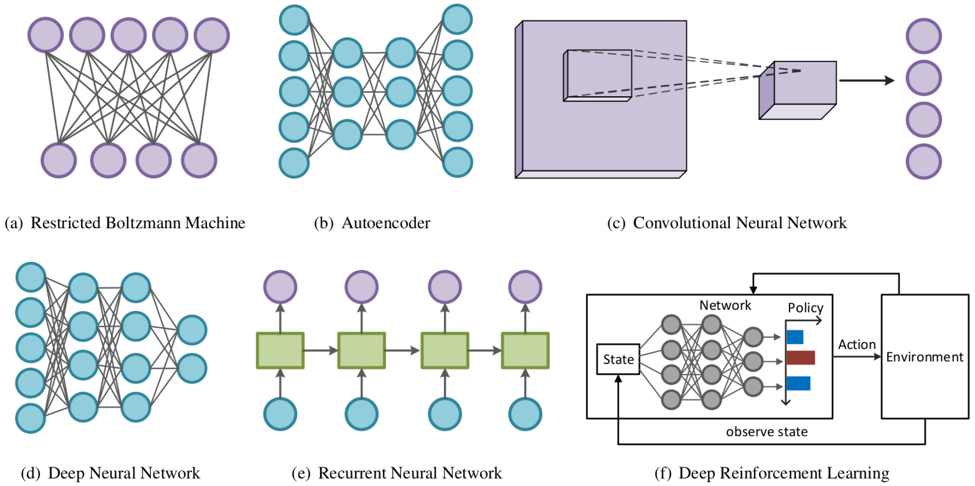
Deep Neural Networks (DNNs) approximate complex nonlinear functions through a composition of hierarchical layers. As depicted in Figure 6, different architectures are specialized for robotic tasks: Convolutional Neural Networks (CNNs) [36] utilize spatial kernels to process visual feedback for perception; Recurrent Neural Networks (RNNs) [37] maintain internal states to account for temporal sequences in dynamic modeling; and Multi-Layer Perceptrons (MLPs) [38] are frequently employed to represent control policies. The recursive definition of a standard feedforward hidden layer is given by
where:
- denotes the layer index in an L-layer network.
- is the vector of activations for layer l, with as the input.
- and are the weight matrix and bias vector of the l-th layer, respectively.
- is a nonlinear activation function, such as the Rectified Linear Unit (ReLU) [39], which enables the network to approximate non-convex functions.
Figure 6.
The structures of different deep learning models used in robotics: CNNs are typically used for visual feature extraction, while RNNs and MLPs are used for dynamics and policy approximation (picture courtesy of [40]).
To better contextualize the role of Deep Neural Networks within synergistic robotic frameworks, it is useful to map their function onto a classical closed-loop control block diagram. Rather than directly synthesizing the control policy itself, data-driven Deep Learning architectures are most often employed to improve system perception and dynamics modeling. In this sense, they can be viewed as advanced system identification tools that help infer unmodeled friction, actuator degradation, and complex environmental interactions from raw sensory input. Accordingly, Deep Learning is often associated with the Plant or State Estimator components, where it contributes to translating physical behavior into a usable mathematical state representation for downstream planning algorithms.
To support these perception and modeling roles, modern robotic architectures employ specialized network structures tailored to different sensory modalities. Multi-Layer Perceptrons are commonly used for direct value function approximation and latent mapping in low-dimensional state spaces, where they efficiently transform established kinematic states into representations that are more convenient for the controller [41]. By contrast, Convolutional Neural Networks provide a natural bridge for high-dimensional visuomotor control. By compressing raw pixel data into compact latent representations, this form of dimensionality reduction enables downstream algorithms to process complex, unstructured environments without relying on manual feature engineering [5].
Furthermore, because physical robots operate continuously in the real world, Recurrent Neural Networks and Long Short-Term Memory networks are especially valuable for partially observable environments and time-varying unmodeled dynamics [37]. By maintaining internal hidden states across sequential time steps, these architectures can implicitly capture temporal dependencies. This capability allows the overall control system to better compensate for sensor latency, external disturbances, and friction variations that traditional static models may not represent adequately.
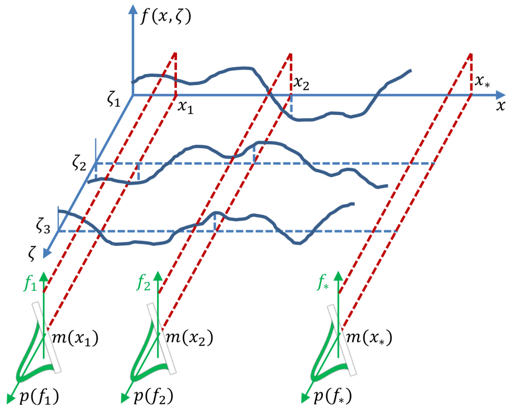
Gaussian Processes (GPs) offer a non-parametric Bayesian alternative. Unlike DNNs, which provide a point estimate, a GP defines a distribution over functions . Here, is the mean function representing the expected value at input , and is the covariance (kernel) function that encodes the spatial correlation and smoothness assumptions of the underlying process.
As illustrated in Figure 7, the GP represents a collection of random variables, where any finite number of these variables have a joint Gaussian distribution. At specific test points and , the model provides marginal distributions and (depicted as green Gaussian curves) centered at their respective mean values . The spreads of these curves explicitly quantify the predictive uncertainty.
The predictive equations are given by
where the parameters are defined as follows:
- is the test input vector where a prediction is desired.
- is the vector of observed noisy training targets.
- is the covariance (kernel) matrix of the training inputs, where .
- is the covariance vector between the training inputs and the test input .
- is the kernel function (e.g., Squared Exponential) that encodes the smoothness of the function.
- is the variance of the additive Gaussian noise in the observations.
- is the identity matrix of appropriate dimensions.
This explicit uncertainty quantification enables safe exploration, allowing a robot to distinguish between known dynamics and unmapped, high-variance state-space regions [42,43]. While the foundational framework for GPs is established in [44], its application to safety-critical robotics relies on using to constrain the controller within regions of high model confidence.
Figure 7.
Visualization of a Gaussian Process as a distribution over functions: The blue lines represent sample realizations of the process , while the green bell curves illustrate the marginal Gaussian distributions at specific points and , with spreads determined by the local predictive uncertainty (picture courtesy of [45]).
2.2.2. Reinforcement Learning (RL)
Reinforcement Learning (RL) [46] addresses sequential decision-making in environments with unknown dynamics. It formalizes the robot’s task as a Markov Decision Process (MDP) defined by the tuple , where:
- and are the sets of all possible states (the robot’s situation) and actions (the robot’s choices).
- P is the transition probability, representing the likelihood of moving from one state to another given a specific action.
- R is the reward function, which provides numerical feedback for the robot’s performance.
- is the discount factor, which determines the importance of future rewards compared to immediate ones.
The goal is to learn a policy , a strategy that maps states to actions that maximizes the expected discounted cumulative return such that
where represents a trajectory (a sequence of states and actions) and is the reward received at time t.
As a practical example, consider a quadrotor learning to stabilize its flight. The state comprises the vehicle attitude and angular velocities, while the action represents the commanded rotor thrusts. The reward function would provide a positive scalar value for minimizing the trajectory tracking error, penalized by excessive control effort or energy consumption. The discount factor ensures the quadrotor prefers achieving a stable hover quickly rather than oscillating over time.
Building upon the state representations produced by the aforementioned Deep Learning modules, Reinforcement Learning plays a complementary yet distinct role within the classical control block diagram. Rather than focusing on modeling the physical plant, Reinforcement Learning is primarily concerned with decision making and control policy improvement. By optimizing the expected cumulative reward through sequential interactions, it provides a data-driven framework for approximating optimal control strategies. In this context, Reinforcement Learning can be viewed as augmenting, and in some cases partially replacing, the traditional Controller block [47]. It computes control actions based on the estimated states, thereby completing a unified architecture in which Deep Learning enhances perception and modeling, while Reinforcement Learning contributes to adaptive and task-driven control.
- Model-Free vs. Model-Based RL
In Model-Free RL, the agent learns directly from experience without trying to understand the underlying physics. For example, Q-learning updates the action-value function which represents the expected total reward for taking action in state , based on the following Bellman equation:
where represents the next state the robot enters after performing action , and represents the best possible future value the robot can achieve from that next state.
To provide intuition, imagine an Autonomous Surface Vehicle tracking a complex trajectory in a dynamic environment. If the vehicle is currently at a specific coordinate and heading (state ), it must decide whether to adjust its rudder angle (action ). The Q-function evaluates this specific steering action. It outputs a scalar value representing not just the immediate stability of the turn, but the complete expected trajectory quality, ensuring the vehicle maintains optimal tracking performance for the remainder of the mission.
Policy Gradient methods, such as Proximal Policy Optimization (PPO) [48], directly optimize the policy parameters by estimating the gradient . While capable of learning complex behaviors, these methods suffer from high sample complexity. This means they require an enormous amount of data, often millions of trial-and-error interactions, to learn a simple task. For instance, a robot might need to “crash” thousands of times in a simulation before it learns to balance, which is often impractical for real-world hardware.
In Model-Based RL, the agent explicitly learns a transition model and uses it for planning. This drastically improves sample efficiency but introduces “model bias”; if the learned model is slightly wrong, the robot may incorrectly exploit these errors, leading to failure in real implementation [11,46].
- Deep Reinforcement Learning (DRL)
As shown in Figure 8, Deep Reinforcement Learning (DRL) replaces traditional tabular value functions with neural networks. The “Agent” (i.e., the neural network policy) observes the “State” (e.g., joint angles, sensor readings) and outputs an “Action” (e.g., motor torques). The “Environment” returns a “Reward” signal indicating success. This creates a closed-loop learning system where the Agent improves through continuous trial and error.
Figure 8.
DRL applied to a robotic manipulator: The neural network agent interacts with the environment (through trial and error) to maximize a reward signal, learning a state-to-actions mapping (picture courtesy of [49]).
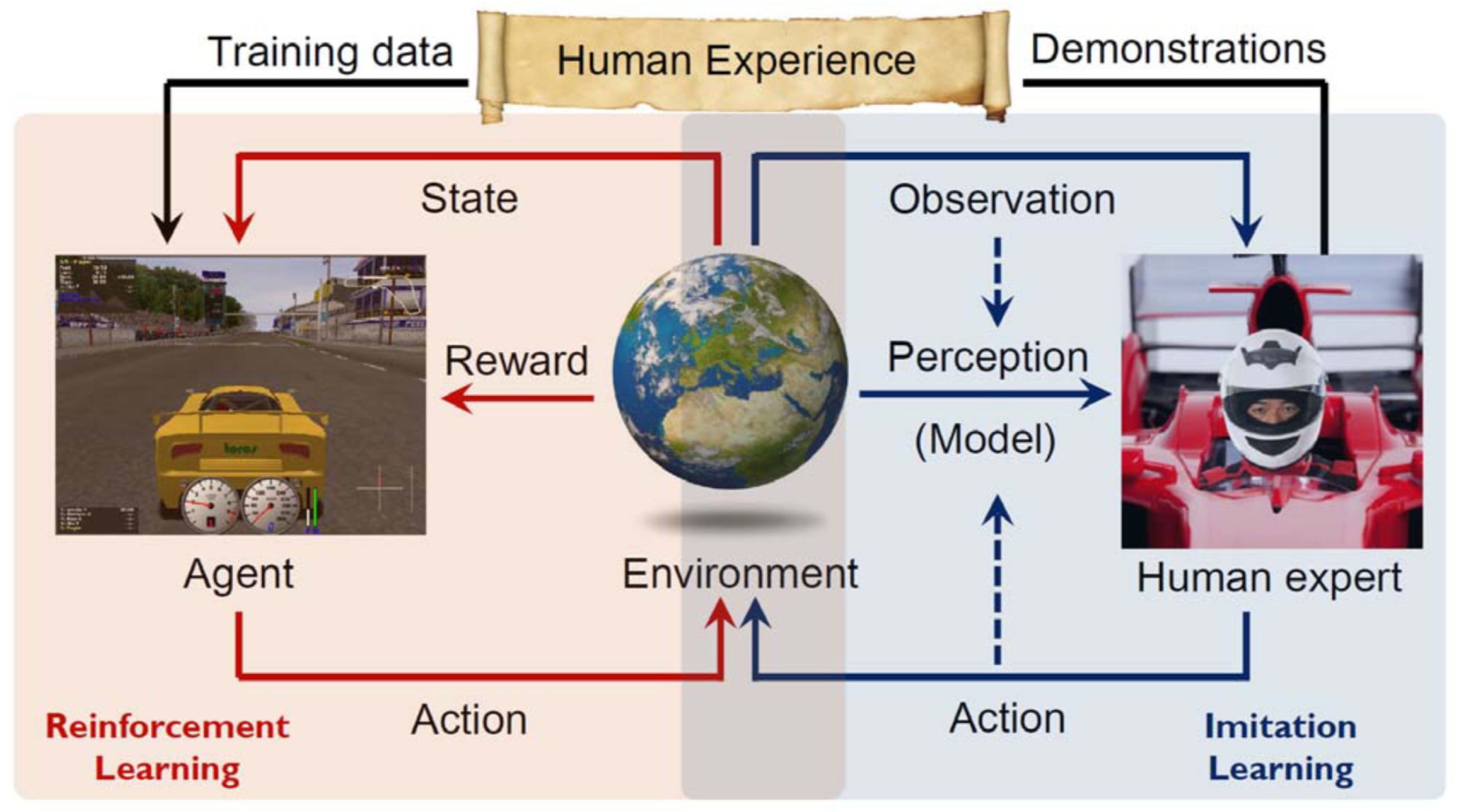
2.2.3. Imitation Learning (IL)
Reinforcement learning relies on a well-defined reward function, which can be difficult to specify for complex behaviors (e.g., “driving politely” or “walking gracefully”). Imitation Learning (IL) bypasses this complexity by learning directly from a dataset of expert demonstrations [50,51]. The interaction between human experts and the learning agent is depicted in Figure 9.
- Behavioral Cloning (BC)
Behavioral Cloning (BC) treats control as a supervised learning problem [52]. It trains a policy to minimize the difference, , between its actions and the expert’s actions such that
where:
- is the expert dataset consisting of state-action pairs .
- is the agent’s policy parameterized by weights .
- denotes the squared Euclidean distance, which penalizes large deviations from the expert’s chosen action.
While simple to implement, BC suffers from covariate shift, which is where small errors accumulate and push the robot into states not seen in the training data and, thus, where the policy is undefined. This occurs because the robot’s small execution errors lead it into states not covered in ; since the policy was never trained on these “off-trajectory” states, the errors compound, often leading to catastrophic failure [53].
- Inverse Reinforcement Learning (IRL)
Inverse Reinforcement Learning (IRL) addresses the limitations of BC by inferring the expert’s underlying reward function rather than simply imitating raw actions [54]. This is typically formulated as a bi-level optimization problem [55]:
- Inner Level (Policy Optimization): For a given reward function, the agent solves an RL problem to find the optimal policy .
- Outer Level (Reward Learning): The reward function is updated to maximize the margin between the expert’s performance and that of all other possible policies.
A common formulation of IRL is Maximum Entropy IRL [56], which assumes the probability of a trajectory is proportional to its total reward. The probability is defined as
where represents a full sequence of states and actions. This framework allows the robot to learn the intent behind the behavior, facilitating better generalization to new environments [12].
Figure 9.
The framework of RL, IL, and their integration: Human expert demonstrations can pretrain a model, shape the reward function, or guide the exploration of the RL agent (picture courtesy of [57]).
3. Applications to Robotic Platforms
The integration of control-theoretic structure with learning-based adaptability has matured across several representative robotic domains. Each platform presents distinct physical challenges—ranging from underactuated dynamics to high-dimensional perception and contact uncertainty—that motivate specific hybrid designs. This section surveys how synergistic control-learning frameworks have advanced state-of-the-art performance in five major platforms: legged locomotion, Uncrewed Aerial Vehicles (UAVs), robotic manipulators, Uncrewed Ground Vehicles (UGVs) and marine robotic vehicles.
3.1. Legged Locomotion
Legged robots have long served as the proving ground for the unification of analytical control and data-driven learning. Since Raibert’s seminal work on dynamic balance control for hopping robots [58], the field has evolved from early reduced-order templates, such as the Spring-Loaded Inverted Pendulum (SLIP), to full-body, optimization-based controllers capable of taking into account multi-contact transitions, uneven terrain, and dynamic disturbances. Modern platforms such as that of MIT Cheetah [2] and ANYmal [3] have pushed the frontier by demonstrating that high-speed locomotion, robust recovery maneuvers, and adaptive terrain negotiation can all be achieved when model-based structures and data-driven adaptation are combined effectively.
Model-based strategies, such as Whole-Body Control (WBC) and MPC, remain central to enabling real-time stabilization and constraint satisfaction on platforms such as MIT Cheetah (shown in Figure 10). These approaches leverage rigid-body dynamics, task hierarchies, and explicit contact constraints to compute precise torque or force commands. The strength of these approaches lies in interpretability and strong performance guarantees that have enabled reliable execution of complex behaviors (e.g., dynamic trotting, bounding, and galloping). However, the reliance on simplified models (including approximate ground contact assumptions, linearized friction cones, and nominal actuator models) limits performance under severe modeling uncertainty, actuator degradation, and time-varying terrain properties.
Figure 10.
The MIT Cheetah 3 Robot during galloping motion (picture courtesy of [2]).
Learning-driven methods [59] complement these limitations by capturing latent and nonparametric dynamics that are difficult to explicitly represent with analytic models. The work of Hwangbo et al. [3] demonstrates that simulation-trained policies can produce highly agile locomotion on the ANYmal quadruped, achieving robust sim-to-real transfer even in the presence of significant terrain variability. These results highlight the fact that neural networks naturally absorb complex factors (e.g., ground compliance, actuator hysteresis, and multi-contact nonlinearities) that challenge classical modeling approaches. The foundational work of Rapid Motor Adaptation (RMA) [48] first demonstrated real-time online adaptation for legged robots. In particular, this decoupling framework separated online context inference (i.e., estimating a latent variable that summarizes changes in terrain and robot dynamics from recent proprioceptive history) from the control policy and conditions itself on the context inference to select actions. Subsequent advances, often built upon this decoupling framework, further improved the approach by introducing hierarchical learning architectures and Residual RL (RRL). These advances incorporated physics-based a priori knowledge into DRL frameworks, leading to more robust policies and significantly improving sample efficiency. Such approaches benefit from the structure of model-based components while still retaining the flexibility of learned dynamics.
A promising approach in legged locomotion research is hybridization: combining model-based controllers that enforce feasibility, stability, and constraints with learning modules that correct model discrepancies in real time. Residual-learning-enhanced MPC [60] provides a representative example of this approach, where the nominal dynamics used for prediction and constraint enforcement remain fixed, while a learned residual model updates local dynamics to improve accuracy in challenging terrains. On wheeled–legged platforms, hybrid frameworks have been used to jointly design gait schedulers and low-level torque controllers, improving terrain adaptability, slip compensation, and overall energy efficiency [61]. These systems demonstrate that physics-based structure is essential for safety, predictability, and sim-to-real reliability, while learned components provide the agility and robustness needed to operate effectively in unstructured environments.
Recent works further advance the hybrid paradigm in legged locomotion. Nguyen et al. [62] proposed a variable-frequency residual dynamics learning and real-time MPC framework on Unitree A1. They showed that by learning a residual model from hardware data and using different time resolutions for contact and flight phases within MPC, their approach improved the tracking accuracy and robustness of long-flight jumping (including continuous jumps) over uneven, unstructured terrain. These studies highlight the efficacy of integrating learning-based predictive models within model-based controllers to take into account unmodeled dynamics and environmental variability.
Expanding beyond quadrupedal and wheeled legged systems, humanoid robots have emerged as a premier frontier for the integration of modern control theory and machine learning. Unlike specialized platforms, humanoids must concurrently manage complex locomotion, dynamic balance, and manipulation. This complexity typically necessitates a hierarchical synergy where model-based techniques, such as Whole Body Control (WBC), Inverse Dynamics, and MPC, are deployed at the lower level to ensure real time stability and constraint satisfaction. Concurrently, data-driven components, including Reinforcement Learning (RL), Imitation Learning (IL), and foundation models, occupy the higher levels for task planning and adaptive gait generation. Furthermore, an increasingly prominent alternative bypasses this hierarchy entirely by utilizing end-to-end reinforcement learning to directly map sensory observations to continuous control commands for robust humanoid locomotion [63,64]. Recent advancements in platforms like Tesla Optimus, Boston Dynamics Atlas, and Unitree G1 signify a transition from laboratory prototypes to industrial deployment in logistics and manufacturing. However, achieving dexterous manipulation and efficient transfer from simulation to reality for systems with many degrees of freedom remains a critical challenge. As such, humanoid robotics serves as a definitive proving ground for architectures that fuse the analytical stability of classical control with the adaptive intelligence of machine learning.
Overall, recent research in legged locomotion exemplifies the broader trend observed across robotic platforms: the integration of model-based methods that ensure stability and safety with data-driven components that enhance adaptability and performance. The resulting hybrid architectures represent a powerful paradigm for achieving versatile and high-performance locomotion in real-world settings.
3.2. Uncrewed Aerial Vehicles (UAVs)
Uncrewed Aerial vehicles represent another arena where hybrid learning–control systems have shown exceptional promise. Quadrotors and fixed-wing UAVs exhibit fast, nonlinear, and tightly-coupled dynamics. Here, even small modeling errors can cause rapid instability or significant tracking failures. The underactuated nature of these systems, combined with their rapid timescales and sensitivity to aerodynamic disturbances, requires UAV controllers that are both highly responsive and robust to unmodeled dynamics. Classical nonlinear control and MPC frameworks provide provable guarantees of stability, the satisfying of constraints, and the existence of feasible trajectories. But their level of accuracy and performance are dependent upon their aerodynamic models, which are difficult to characterize under real-world disturbances (e.g., wind gusts, ground effects, rotor wake interactions, and structural flexibilities). Hybrid architectures are ideal for UAVs, where a model-based structure ensures feasibility and stability while learning-based components maintain high performance in real-world environments.
Learning-enhanced controllers mitigate the limitations of traditional control methods by modeling unknown forces and being able to accommodate new flight regimes. Bouffard et al. pioneered one of the earliest learning-based MPC frameworks for quadrotors, incorporating data-driven model updates to reduce the mismatch between predicted and actual dynamics [65]. This strategy improved prediction fidelity without compromising the structure of MPC, enabling safer and more accurate flight in complex environments. More recent adaptive MPC formulations further demonstrated that online estimation of aerodynamic parameters can enhance tracking performance under rapidly changing flow conditions [66]. In parallel, Torrente et al. extended this line of work by introducing a fully data-driven MPC approach in which neural network regressors completely replaced all analytic models and, as a result, achieved centimeter-level tracking accuracy during agile maneuvers [67]. Their results highlighted the potential of learned dynamics to capture intricate aerodynamic effects (e.g., rotor drag, attitude–translation coupling, and nonlinear thrust saturation) that traditional models have difficulty in fully capturing.
Residual learning architectures further complement MPC by learning unmodeled disturbances such as turbulent wind fields, propeller saturation effects, or platform-specific nonlinearities. The Neural-Fly framework exemplified this trend (shown in Figure 11). By deploying a lightweight neural residual model trained online, it achieved high-speed flight in strong and unpredictable wind conditions [4]. The hybrid design maintained a physically interpretable, constraint-aware-based model for prediction and control, while the learned residual term adapted rapidly to changing aerodynamic conditions. This separation of structure to allow for both stability and high performance in an adversely changing environment has become a defining characteristic of modern UAV control.
Figure 11.
Agile flight through narrow gates. (A) Caltech Real Weather Wind Tunnel system. (B,C) Trajectories used for the gate tests. (D,E) Long-exposure photos (with an exposure time of 5 s) showing one lap in two tasks. (F–I) High-speed photo (with a shutter speed of 1/200 s) showing the moment the UAV passed through the gate and the interaction between the UAV and the wind (picture courtesy of [4]).
The synergy of learning and structure has also extended to perception. End-to-end visuomotor policies (i.e, policies that coordinate motion with visual perception) pretrained in simulation and refined via structure-imposing control have demonstrated the ability to take into account sensor noise, lighting variations, and dynamic obstacles [68]. Complementary work on UAV racing shows that learned perception modules combined with MPC-based guidance can achieve human-level agility in visually complex environments [69]. These studies highlight a common trend: perception and low-level control remain grounded in analytic structure, while learning takes into account visual ambiguity, aerodynamic disturbances, and distribution shift. Collectively, in light of these developments, UAVs are a prime example of how learning can augment rather than replace model-based flight control to enable real-time high-speed, high-performance flight in the face of time-varying, environmental disturbances and uncertainties.
3.3. Robotic Manipulators
Robotic manipulators face distinctive challenges due to contact physics, frictional coupling, and object variability. Unlike locomotion or flight, manipulation must address intermittent contact, stick–slip transitions, deformable objects, and diverse tasks from precision assembly to unstructured human environments. Model-based approaches (e.g., impedance control and MPC) provide stability, passivity, and clear safety guarantees, enabling compliant interaction with the physical world. Yet, modeling issues such as frictional impacts, complex contact geometries, and material deformation result in discontinuous dynamics that are difficult to parameterize. These complexities limit analytic model fidelity and often result in tracking errors or overly conservative policies.
Learning-based methods complement these tools by capturing nonlinearities that are difficult to model. However, these methods alone typically lack guarantees of constraint satisfaction or safe exploration. Pure DRL policies remain sample-inefficient and brittle in contact-rich settings, where small perturbations can cause large behavioral deviations. This tension between the principled model-based structure and the flexibility of machine learning motivates hybrid approaches that combine the strengths of both paradigms.
Hybrid control–learning frameworks currently play a central role in manipulation. Guided Policy Search (GPS) [5] alternates local model-based optimizations with supervised policy updates, enabling end-to-end training of deep visuomotor policies while anchoring learning in stable analytic controllers. RRL [6] follows a similar philosophy. That is, a nominal controller ensures safety; and a learned residual provides adaptive corrections, enabling rapid adaptation to changing object properties and disturbances while reducing data requirements by avoiding unsafe exploration.
Structured neural architectures further enrich these hybrids frameworks. Graph Neural Networks (GNNs) encode spatial and relational priors (i.e., relationships known a priori) among objects and robot links, producing dynamic models that are versatile enough to take into account varying geometries, contact modes, and multi-body configurations [70]. Embedded into hybrid MPC frameworks, GNNs support accurate prediction and real-time control of deformable, articulated, and soft objects while preserving MPC’s constraint satisfaction and interpretability. That is, control actions are directed to follow explicit optimization objectives and hard constraints [71].
Similar work has addressed sim-to-real transfer for contact-rich manipulation. Inaccurate contact models, friction coefficients, and stiffness parameters create domain gaps that hinder the direct transfer of simulation-trained policies. To mitigate this reality gap, many studies use dynamics randomization, compliant force/impedance control, and high-fidelity contact simulation. Randomizing masses, friction, and other dynamics parameters improves performance for planar pushing and locomotion tasks [72]. OpenAI’s dexterous in-hand manipulation system demonstrated that large-scale domain randomization over physical and visual properties are sufficient to transfer high-dimensional policies to a Shadow Hand without real-world demonstrations (shown in Figure 12) [73]. Building on these ideas, Zhang et al. introduced a hybrid offline–online framework with online admittance residual learning that adapted compliance parameters from force/torque feedback. This framework achieved efficient sim-to-real transfer for assembly, pivoting, and screwing motions while preserving the structure of an admittance controller (i.e., a controller that maps measured force/torque feedback to compliant motion commands such as that for desired Cartesian velocity or pose) [74]. Together, these works have demonstrated that combining structured compliance control with domain randomization and online adaptation yields reliable and high-performance transfer in contact-rich manipulation.
Figure 12.
OpenAI’s dexterous in-hand manipulation in virtual and real environmental tests (Red circle shows three-camera setup for vision-based state estimation) (picture courtesy of [73]).
Overall, these developments indicate that structured learning is a powerful complement to analytical models. By respecting contact constraints, physical symmetries, and task-specific structure, hybrid manipulation systems can achieve both robustness and interpretability. This combination is crucial for industrial deployment, autonomous assembly, and safe human–robot collaboration.
3.4. Uncrewed Ground Vehicles (UGVs)
The operation of autonomous Uncrewed Ground Vehicles (UGVs) epitomizes the complexity of hybrid decision and control in dynamic, uncertain, and multi-agent environments. Roadway interactions involve pedestrians, human-driven vehicles, cyclists, and other autonomous agents whose behaviors are inherently stochastic and context-dependent. Traditional motion planning separates behavior prediction, trajectory optimization, and low-level control [1]. This modularity offers transparency and interpretability, enabling engineers to diagnose failures and certify safety. That is, decisions can be traced to explicit prediction, cost functions, constraints, and control laws rather than opaque end-to-end mappings. However, these systems struggle with non-stationary human interactions, distribution shift in traffic behaviors, and long-horizon uncertainty challenges that often cause unreliable or overly conservative driving decisions when relying solely on handcrafted models (e.g., rule-based behavior descriptions and fixed interaction templates).
Learning components enhance these pipelines by improving prediction accuracy and adaptability. Large-scale datasets such as the Waymo Open Motion Dataset [75] and nuScenes have enabled deep neural models capable of predicting multimodal, socially compliant trajectories for surrounding road users. The resulting predictors have captured subtle interaction cues—yield behavior, intent changes, or cooperative maneuvers—that classical models cannot easily encode. Sample interactions are shown in Figure 13. In hybrid architectures, the learned intent predictors are integrated into model-based planners to augment cost maps, refine feasible sets, and provide probabilistic constraints. Consequently, the UGVs (i.e., the autonomous agents being controlled) can exhibit behavior that is both socially aware and compatible with verifiable optimization frameworks, providing a principled balance between versatility in changing environments and safety.
Figure 13.
Examples of interactions between agents in a scene in the WAYMO OPEN MOTION DATASET (picture courtesy of [75]).
At the control level, learning-augmented MPC schemes exploit data gathered over repeated task executions to refine terminal sets and terminal costs, thereby improving performance while satisfying given constraints and preserving recursive feasibility. For example, if the MPC optimization problem is feasible at the current time step, then after applying the first control input of the computed solution, the optimization remains feasible at the next time step and, thus, for all subsequent steps under the same update law [76]. In the Learning MPC framework of Rosolia and Borrelli, trajectories from previous iterations were used to construct a safe set and data-driven terminal cost, enabling constrained vehicle-like systems in iterative driving tasks to progressively approach optimal behavior without requiring an accurate reference trajectory or fully a priori known dynamics. By updating terminal cost and local models from data, such learning-enhanced MPC controllers can better accommodate modeling errors and strict constraints while retaining the optimization-based structure of MPC used for constraint enforcement. RL agents are further constrained by Control Barrier Functions (CBFs) to enforce strict safety constraints such as those for collision avoidance, road boundaries, and minimum stopping distances [16]. These safety filters ensure that learned policies remain within certified safe sets during both training and deployment, preventing catastrophic failures while allowing exploratory learning.
Hybrid decision–control frameworks thus represent a blueprint for the broader robotics community, closely aligned with the hybrid taxonomy to be introduced later in this survey. They maintain a verifiable model-based foundation for safety, interpretability, and regulatory compliance, while leveraging data-driven learning to extend autonomy, flexibility, and efficiency in complex real-world settings. This fusion supports long-horizon driving strategies that can accommodate dynamic, multi-agent interactions, address uncommon or ambiguous behaviors, and generalize across diverse driving domains. As such, autonomous vehicles demonstrate how hybrid architectures can simultaneously achieve resilience, scalability, and high-performance decision-making in safety-critical applications.
3.5. Marine Robotic Vehicles
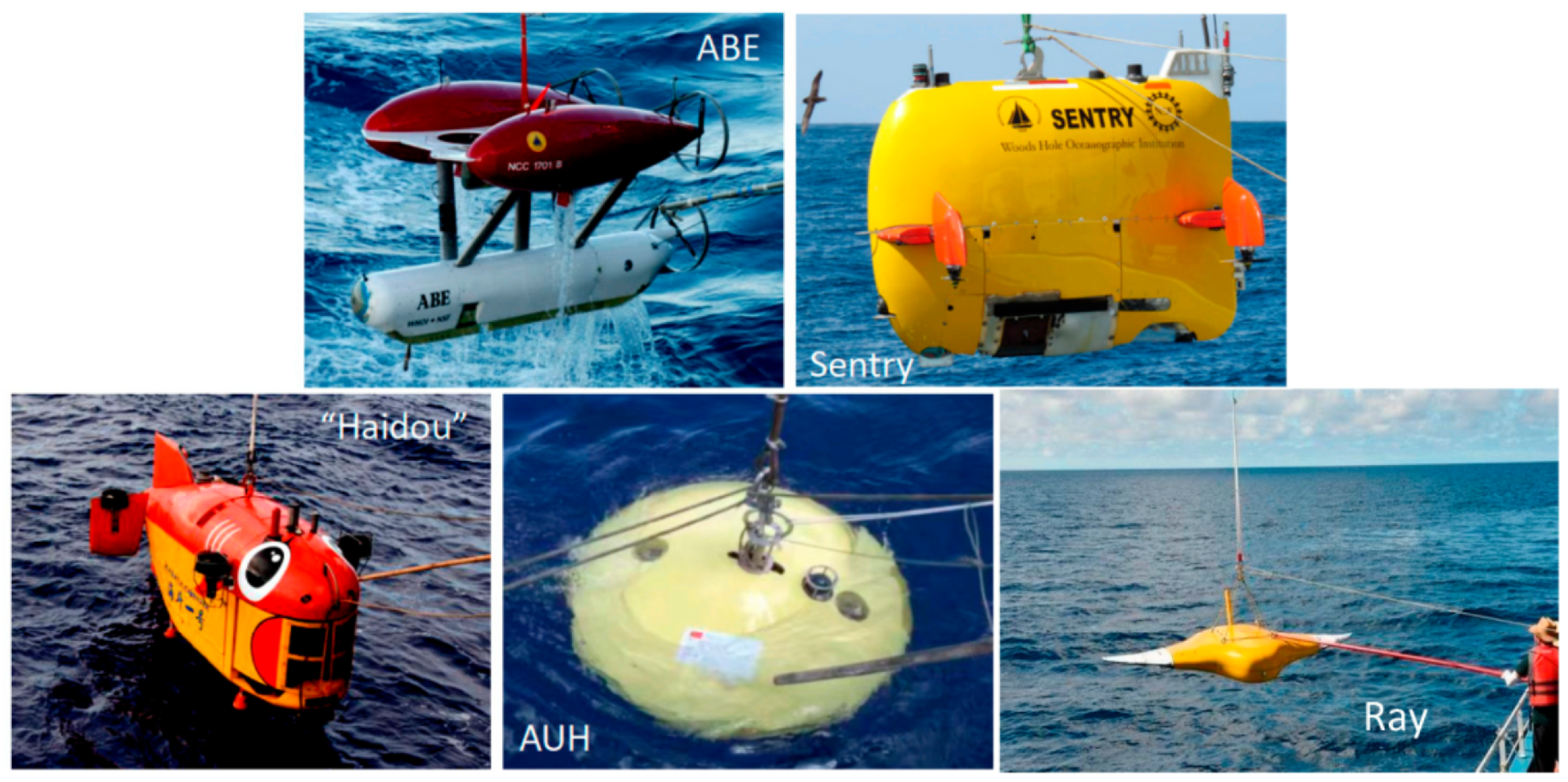
Marine robotic vehicles—including autonomous Uncrewed Underwater Vehicles (UUVs), Autonomous Surface Vehicles (ASVs), and Remotely Operated Vehicles (ROVs)—operate in fluid environments that are disturbance-rich, only partially perceivable, and strongly nonlinear. Example AUVs are shown in Figure 14. Their dynamics involve added mass, viscous drag, and unsteady flow effects that vary with speed, proximity to boundaries, and sea state. Consequently, traditional guidance and control still rely on physics-grounded 6-DOF marine craft modeling as the nominal foundation for stability and interpretability, with Fossen’s formulation remaining the canonical model for Guidance, Navigation and Control (GNC) design in both surface and underwater platforms [77]. However, purely analytic models often fail to capture, for example, mission-specific hydrodynamic residuals or rapidly changing current–wave interactions.
Hybrid learning–control methods address these gaps by estimating unmodeled forces while preserving the structure of nominal dynamics. Early and influential work demonstrated that neural networks can augment underwater vehicle model identification by learning residual hydrodynamic terms in addition to physics-based equations, thus improving prediction accuracy and control performance under uncertain flow conditions [78]. For AUVs, learning-based observers and data-driven maneuvering models have similarly been used to infer nonlinear current-induced effects and time-varying disturbances during path-following and station-keeping, enabling accurate control even with input saturation and limited onboard sensing [79]. These approaches function as “drop-in” corrections to Fossen-style models, maintaining interpretability while increasing fidelity in real deployments.
Figure 14.
Various body structures of the seabed AUVs (picture courtesy of [80]).
Beyond deterministic residual learning, probabilistic models provide robustness by quantifying disturbance uncertainty. Gaussian process regression has been integrated with robust controllers to learn wave/current effects online and deliver uncertainty-aware compensation in real time. This framework yields improved dynamic positioning and trajectory tracking in underwater robots [81]. Safety-critical missions (e.g., close-proximity inspection, docking, and operation near fragile infrastructures) and the need to react to harsh and changing environments further motivate hybrid architectures that enforce hard constraints while allowing local adaptation. Recent safety-critical AUV control systems have combined a model-based core with neural function approximation of unknown disturbances to ensure constraint satisfaction under environmental uncertainty [82]. Furthermore, differentiable simulation has enabled novel end-to-end co-design strategies. Differentiable hydrodynamics enables gradients to propagate through fluid–structure interactions, meaning that task objectives (e.g., tracking error or energy consumption) can be differentiated with respect to control inputs and physical/model parameters, thereby enabling gradient-based optimization of both design and control for marine robotic vehicles [83].
Overall, the application of Learning-for-Control to marine robotic vehicles in safety-critical, high-fidelity domain allows for: (1) structured hydrodynamic models to provide stability and constraints, alongside (2) learned residuals, probabilistic disturbance models, and differentiable simulators to supply the adaptability needed for unsteady real-world oceans.
3.6. Comparative Discussion Across Robotic Platforms
The five robotic platforms discussed in this paper exhibit distinct balances between model fidelity, environmental uncertainty, and safety requirements, leading to different hybrid control–learning designs. As summarized in Table 1, aerial robots and autonomous vehicles rely heavily on accurate dynamic models and strict safety guarantees. Learning, therefore, is primarily used to model disturbances or predict multi-agent interactions without compromising required constraints. Marine robots share this emphasis on safety and model fidelity but operate in fluid environments characterized by unsteady hydrodynamics and limited sensing, making online disturbance compensation essential.
Table 1.
Consolidated cross-platform comparison of hybrid control–learning requirements.
Legged locomotion and robotic manipulators operate in regimes where analytic modeling is limited by contact events, friction, and structural variability. Here, learning contributes by capturing unmodeled physics, enriching dynamics representations, and adapting to terrain or object changes, while model-based controllers preserve stability and constraint satisfaction. Manipulators uniquely benefit from structured representations (e.g., graph-based contact models), while legged locomotion leverages residual learning for terrain versatility.
Hybrid strategies are implemented to reflect their corresponding domain properties. Residual learning with MPC or whole-body control is common in legged systems. Learning-enhanced MPC is common in UAV platforms. Manipulators integrate learned contact models into impedance or MPC frameworks. Marine robotic vehicles employ learned hydrodynamic residuals or Gaussian-process disturbance models to complement nominal fluid-dynamics equations. Autonomous UGVs combine learned prediction modules with constraint-aware planners, such as MPC or CBFs. Safety requirements further differentiate the platforms, ranging from very high in UAVs, marine robots, and autonomous UGVs, to moderate levels in legged and manipulator systems. Overall, the comparison indicates that high-fidelity, safety-critical platforms favor Learning-for-Control architectures; while domains with discontinuous or variable dynamics benefit more from model-augmented or residual learning. Regardless, across all five areas, hybrid approaches consistently provide superior performance compared with that of either purely model-based or purely data-driven methods alone.
4. Multi-Agent Reinforcement Learning (MARL) in Robotics
Many robotic systems in practice, from cooperative mobile robots and UAV teams to swarm platforms, operate in multi-agent settings where coordination, communication, and decentralized decision-making are central challenges. This has motivated the rapid development of Multi-Agent Reinforcement Learning (MARL). Among the foundational works shaping modern MARL, Proximal Policy Optimization (PPO) and its multi-agent variant Multi-Agent PPO (MAPPO) [48,84] have provided a stable on-policy actor–critic framework that optimizes a clipped surrogate objective such that
where . Here, denotes the stochastic policy parameterized by , while represents the policy used to generate the data. The ratio measures the relative change in action probability under the updated policy. The advantage estimate evaluates the relative quality of action taken in state , and is a hyperparameter that constrains the maximum allowable deviation between the new and old policies. The operator restricts the probability ratio to the interval .
The clipped surrogate objective limits policy updates by preventing excessively large changes in action probabilities. For positive advantages, the objective stops increasing once the probability ratio exceeds , and for negative advantages, it prevents further decreases when the ratio falls below . This formulation yields a conservative approximation of the policy improvement objective and encourages stable learning without requiring explicit constraints. This framework serves to form the basis of many robust continuous control methods for robotic applications.
Value Decomposition Networks (VDN) [85] decompose a global team value (i.e., reward) function into additive per-agent terms, enabling Centralized Training with Decentralized Execution (CTDE). The key idea is to approximate the joint action–value function as an additive decomposition of agent-wise value functions, each conditioned only on local observations and actions. VDN enables agents to infer how to maximize the team reward based on their local observations and how their individual actions contribute to the overall team reward. This is important because, in many tasks, the team reward cannot be explicitly decomposed into individual reward signals. Despite these advantages, VDN has notable limitations. For one, VDN relies on a strong assumption of additive value decomposition, which restricts representational capacity and prevents modeling complex inter-agent dependencies when the joint value function is inherently non-additive. Consequently, VDN may fail in tasks that require tightly coupled or nonlinear coordination among agents. Furthermore, although training is centralized, the learned decomposition can struggle to scale effectively to large teams or highly heterogeneous agent populations. These limitations motivated subsequent extensions that relax the additivity assumption by introducing monotonic mixing functions. For example, Q-value Mixing Network (QMIX) [86] extends this approach by learning a monotonic mixing network that allows nonlinear combinations of agent values for more informed coordination. QMIX addresses the primary limitation of VDN by relaxing the strict additive decomposition of the joint action-value function while still preserving decentralized execution. Instead of summing individual agent value functions, QMIX represents the joint action–value function , the global team reward function, as a nonlinear mixing of agent-wise Q-values such that
where is a mixing network conditioned on the global state and is the partial observation o .
To ensure consistency between centralized training and decentralized execution, QMIX enforces the following monotonicity constraint on the mixing function:
Monotonicity implies that increasing any agent’s local action–value cannot decrease the joint action–value. As a result, greedily maximizing each agent’s local Q-function is guaranteed to also maximize the joint Q-function, enabling agents to act independently at execution time.
By introducing a nonlinear but monotonic mixing function, QMIX represents a broader class of joint value functions than VDN, including settings with non-additive but positively correlated agent contributions. However, the monotonicity constraint still limits expressiveness and prevents modeling tasks that require non-monotonic coordination, such as scenarios where improving one agent’s action must reduce another agent’s contribution. This limitation motivated subsequent methods, such as QTRAN [87], which further relax structural constraints on value factorization.
Multi-Agent Deep Deterministic Policy Gradient (MADDPG) [88] advances deterministic policy gradients by employing a centralized critic that observes joint actions during training, thus stabilizing learning in cooperative and competitive multi-agent environments. MADDPG is an actor–critic method that does not rely on value function decomposition. Instead, it employs centralized critics (observers) and decentralized actors (controllers), where each agent learns its own policy while the critic is conditioned by the observations and actions of all agents during training. This design allows MADDPG to directly model inter-agent interactions without imposing structural constraints on the form of the joint value function.
MADDPG primarily addresses the challenge of non-stationarity in multi-agent learning that arises from simultaneously updating multiple agents. By conditioning the critic on the joint action space, the learning environment appears stationary from the critic’s perspective. MADDPG also mitigates the high variance typically observed in policy gradient methods, particularly in coordination tasks, by leveraging centralized critics that provide more informative and stable gradient estimates. Furthermore, MADDPG naturally extends to mixed cooperative–competitive environments in which agents may have different or even opposing reward functions, a setting that is not well-suited for value-decomposition approaches.
Despite these advantages, MADDPG has notable limitations. The centralized critic does not scale well with the number of agents due to the rapidly increasing dimensionality of its input space. It also requires access to other agents’ actions or accurate approximations thereof during training. Moreover, unlike value-decomposition methods, MADDPG does not guarantee that decentralized greedy execution leads to a globally optimal joint policy, and training instability may arise in large cooperative teams.
In summary, value-decomposition methods emphasize scalability and decentralized execution under strong structural assumptions, whereas MADDPG prioritizes representational expressiveness and training stability in complex, interacting, and mixed-reward multi-agent environments.
Another common issue in MARL is the credit assignment problem that arises when multiple agents receive a shared team-level reward, making it unclear how each individual agent’s action contributed to the observed outcome. In fully cooperative settings, a global reward does not provide sufficient information for an agent to determine whether its own action was beneficial or detrimental, since the reward is influenced by the joint actions of all agents. This ambiguity leads to high-variance gradient estimates and inefficient learning, as agents may be rewarded or penalized for outcomes largely driven by other agents’ decisions.
Counterfactual Multi-Agent Policy Gradients (COMA) addresses the credit assignment problem by introducing a counterfactual advantage function. COMA employs a centralized critic that estimates the joint action–value function conditioned on the global state and the joint action of all agents. For each agent, the advantage is computed by comparing the value of the action actually taken to a counterfactual baseline in which that agent’s action is isolated while keeping the other agents’ actions fixed. Formally, the baseline is obtained by taking an expectation over the agent’s action space under its current policy.
This counterfactual baseline isolates the individual contribution of an agent’s action to the team reward, effectively answering the question: how much better or worse was the outcome because this agent chose this action, given that all other agents acted the same? By subtracting this baseline from the joint action–value, COMA provides low-variance, agent-specific advantage estimates while still optimizing a global cooperative objective.
As a result, COMA enables more accurate credit assignment without decomposing the value function or requiring individual reward signals. However, the use of a centralized critic and action marginalization introduces additional computational cost and limits scalability to environments with large action spaces or to multi-agent systems consisting of a large number of agents. A complementary line of work, Mean-Field MARL [89], approximates interactions among large populations of agents by modeling the average effect of neighbors, making it particularly useful for scalable swarm and collective robotic systems.
Together, these algorithms provide the conceptual and algorithmic foundations for modern multi-robot learning. A concise summary of key MARL algorithms used in robotics is presented in Table 2.
Table 2.
Comparison of Key MARL Algorithms for Robotics.
4.1. RL Applications to Multi-Agent Robotic Systems
4.1.1. Navigation and Crowd-Aware Motion
MARL has provided a methodology for learning safe, efficient, and socially acceptable navigation policies in dynamic multi-agent environments and has been one of the earliest successes for robotic applications. Chen et al. introduced Socially Aware Collision Avoidance with Deep Reinforcement Learning (SA-CADRL) [90]. Here, robots learned collision avoidance strategies in human crowds that respect social norms through DRL, achieving real-time performance on mobile robots. Subsequent extensions [90,91,92] incorporated social awareness, group interactions, and predictive models for pedestrians. Beyond crowd navigation, MARL-based decentralized policies have been used for multi-robot navigation under communication constraints and partial observability, where agents coordinate implicitly without explicit message exchange. GNN-based approaches [93] enable each robot to process local observations and neighbor states to learn scalable decentralized control laws. These techniques show that CTDE-trained policies are scalable to unseen team sizes and dynamic environments, making MARL a viable framework for large-scale navigation.
4.1.2. Multi-Aobot Path Finding (MAPF) and Warehouse Coordination
Coordinating large fleets of robots in structured environments, such as those in warehouses or factory floors, is another MARL central application area. Pathfinding via Reinforcement and Imitation Multi-Agent Learning (PRIMAL) [94] introduced a decentralized MARL framework combining IL and RL to generate scalable policies for thousands of robots in MAPF tasks. PRIMAL2 [95] extended this by improving local observation modeling and reward shaping, demonstrating near-linear scalability to more than 2000 agents. Recent works have integrated hierarchical or factorized architectures inspired by VDN and QMIX to coordinate heterogeneous robot teams efficiently in order-picking and logistics tasks [96,97]. Hierarchical MARL [98] and transformer-based models (shown in Figure 15) [99] have further improved coordination efficiency and learning speed in large environments by decomposing decision making into global and local subpolicies. These results indicate that value-decomposition principles and CTDE training are crucial for taking into account large-scale, partially-observable MAPF problems where explicit communication is limited.
Figure 15.
Architecture of transformer-based VDN (picture courtesy of [99]).
4.1.3. Swarm and Formation Control
Swarm robotics presents an extreme form of multi-agent coordination where several homogeneous agents must act cohesively using only local information. Hüttenrauch et al. [100] proposed permutation-invariant, mean-embedding representations to encode local observations in swarm systems. In this approach, observations of neighboring agents are mapped into a latent feature space and aggregated by taking their mean, yielding a fixed-dimensional representation that is invariant to the ordering and number of neighbors. Permutation invariance ensures that the representation does not depend on how agents are indexed, while mean embedding enables scalable learning by summarizing collective information without explicit pairwise interactions. This design allows reinforcement learning policies to generalize across varying swarm sizes and was demonstrated in tasks such as aggregation and pursuit–evasion. Tolstaya et al. [93] used GNNs as differentiable communication channels to learn decentralized controllers capable of accommodating variable team sizes and topologies. These works illustrate how integrating representation learning (e.g., graph message passing) with MARL objectives produces emergent collective behaviors such as flocking, formation keeping, and consensus under noisy conditions. Recent advances also have leveraged mean-field MARL [89] and graph attention networks for large-scale swarms, pointing toward biologically inspired distributed control for hundreds of robots.
4.1.4. Cooperative Manipulation and Aerial Teams
Multi-agent RL has also enabled new levels of coordination among physically coupled agents. Costantini et al. [101] applied MARL to cooperative aerial payload transport, where multiple UAVs learned continuous thrust and attitude adjustments to share load forces while maintaining formation. Similar actor–critic approaches have been used for collaborative object manipulation with multiple robot arms [102] and quadruped teams performing cooperative pushing and carrying tasks [103]. Hierarchical MARL frameworks integrate motion planning at a high level and control at a low level [98], improving long-horizon stability and sample efficiency. Across UAV and manipulator domains, CTDE-based actor–critic methods (PPO/MAPPO, MADDPG) remain dominant due to their ability to model continuous action spaces and take into account coupled dynamics. Safety-enhanced MARL [104,105] introduces constraints and barrier functions for physically grounded deployments.
4.2. Open Challenges and Trends
Despite rapid progress, several hurdles remain. Scalability to multi-agent systems consisting of hundreds of robots has driven interest in mean-field and graph-based MARL [89,93]. Partial observability and communication limits necessitate attention-based message-passing policies that reason over uncertainty. Safety and sim-to-real transfer remain critical bottlenecks for deploying MARL-trained policies on physical robots. Finally, standardized benchmarks such as swarm navigation, cooperative manipulation, and warehouse logistics are essential to evaluate sim-to-real transfer. Recent trends point toward combining MARL with model-based RL and large-sequence models (transformers), moving the field toward more reliable, data-efficient, and adaptable robotic intelligence.
5. A Taxonomy of Integration Strategies
As the boundaries between classical control theory and modern machine learning grow blurrier, a structured framework is essential to understand the diverse design patterns of hybrid systems. Rather than viewing these fields as competing alternatives, we categorize their intersection into three principal paradigms. This taxonomy is explicitly governed by three markable classification criteria: the direction of structural dependency between the computational modules, the precise functional role assigned to the learning algorithm, and the depth of algorithmic integration. By applying these standards, we define the architecture as Learning-for-Control when the rigorous structure of a classical controller is preserved to guarantee stability and constraint satisfaction, while machine learning acts as a model builder to provide accurate dynamics models, estimate disturbances, or tune hyperparameters. Conversely, we define the paradigm as Control-for-Learning when these roles are reversed. In this case, a learning agent serves as the primary decision maker, but its learning process is rigorously supervised, guided, and constrained by control theoretic principles to ensure stability and data efficiency. Finally, methods are classified as Co-Designed-Architectures when control optimization problems are embedded directly as differentiable layers within neural networks. This deepest level of integration creates a unified computational graph where the entire system can be trained end-to-end.
5.1. Learning-for-Control: “The Model Builder”
In this paradigm, the rigorous structure of a classical controller is preserved to guarantee stability and constraint satisfaction. Machine learning acts as a “model builder,” enhancing the controller by providing accurate dynamics models, estimating disturbances, or tuning hyperparameters. (For this section, MPC is chosen without loss of generality as the example control method in this study.)
5.1.1. Learning-Based MPC (LBMPC)
Classical MPC relies on a nominal model that may fail to capture complex physical phenomena such as aerodynamic drag or contact friction. LBMPC addresses this by decoupling safety from performance. It utilizes a learned oracle (i.e., “black box”) model (e.g., a Gaussian Process or Neural Network) to optimize the performance cost, while simultaneously relying on a robust nominal model to ensure that safety constraints are not violated [106]. The optimization problem solved at each time step is formulated as
where the variables and symbols are defined as follows:
- and are the predicted state vectors (e.g., position, velocity) for the learned and nominal models, respectively.
- is the control input vector (e.g., motor torques).
- is the stage cost, and is the terminal cost, which defines the robot’s objective.
- N is the prediction horizon, or the number of future steps the robot considers.
- ⊕ denotes the Minkowski sum [107], a geometric operation used to augment the nominal state trajectory by the uncertainty set .
- is the bounded uncertainty set, representing the model errors or external noise.
- is the safe set, representing the hard constraints on the state and input (e.g., joint limits or obstacle boundaries).
This dual-model approach allows the robot to use high-performance, complex models for efficiency while the robust nominal model acts as a “safety net” to ensure constraints are never violated [108].
5.1.2. Uncertainty-Aware Dynamics Learning
Standard MPC can be brittle. “Brittle” is a term that describes a lack of structural robustness where the controller performance and stability degrade sharply when subjected to even minor model inaccuracies or environmental states not encountered during training if the learned model is inaccurate. Probabilistic Ensembles with Trajectory Sampling (PETS) addresses this vulnerability by learning a probabilistic dynamics model via an ensemble of bootstrapped neural networks [14]. “Bootstrapping” refers to training multiple independent models on different subsets of the transition data. This approach allows the system to estimate uncertainty in regions of the state space where data is sparse. As illustrated in Figure 16, the system performs trajectory propagation by predicting a distribution over future states rather than a single deterministic path.
Figure 16.
The PETS architecture (picture courtesy of [14]): An ensemble of neural networks learns a probabilistic dynamics model from data (Left), particles are propagated through this model to estimate the distribution of future states (Middle), and an MPC planner uses these distributions to find optimal control sequences (Right).
The MPC planner then optimizes a trajectory that minimizes the expected cost over this entire distribution. This process naturally induces cautious behavior in regions of modeling uncertainty. Because the optimizer accounts for the average cost across all possible outcomes, any action that could lead to a high-cost failure in an uncertain region significantly raises the total expected cost. Consequently, the robot inherently avoids high-variance paths where the model is unconfident and prioritizes safer, well-mapped regions.
5.1.3. Residual Reinforcement Learning (RRL)
As opposed to learning the full dynamics “from scratch”, the Residual Reinforcement Learning (RRL) approach learns a corrective additive term to assist a pre-existing controller. A classical controller (such as a Proportional–Integral–Derivative (PID) [109] or impedance controller) provides a stable “baseline”. An RL agent then learns a residual action to compensate for unmodeled nonlinearities, such as friction or complex contact interactions [6]. The resulting control input is given as
In this formulation, is the current state vector, and represents the learned parameters of the policy. This approach significantly accelerates training because the agent begins with a functional policy, allowing it to focus on refining performance rather than exploring the entire state-action space from a random initialization. Recent studies have shown that this hybrid structure is particularly effective for high-precision tasks such as assembly and contact-rich manipulation [110].
5.1.4. Learning-Based Controller Tuning
While residual methods add a learned term to the control output, another strategy uses ML to tune the internal hyperparameters of the controller itself. Classical MPC is highly sensitive to the tuning of its cost function weighting matrices and and its prediction horizon [111]. The prediction horizon is a critical parameter that dictates how far into the future the controller optimizes, while the weighting matrices balance tracking accuracy against control effort.
As illustrated in Figure 17, the framework proposed by Zhang et al. [111] uses a hierarchical structure where a high-level DRL agent dynamically tunes these parameters online. The agent observes the tracking performance and uses its policy , a mapping that determines the best action based on the current state, to update the MPC parameters such that
where is the observation vector containing the current tracking error, and represents the agent’s policy, which is the strategy used to select the optimal parameters. In addition, is the action, representing the selection of weighting matrices and horizons.
Figure 17.
Hierarchical RL-based tuning framework: An RL agent observes the system state and dynamically adjusts the parameters (e.g., weights or horizons) of the low-level MPC controller to optimize long-term performance (picture courtesy of [111]).
5.1.5. Sliding Mode Control and Machine Learning Integration
Sliding Mode Control (SMC) [112] is a robust nonlinear strategy widely used in robotics to reject uncertainties and environmental disturbances. The dynamic model of a robotic system is generally expressed as
Here, is the state vector, is the control input vector, and represent the known nominal dynamics, and encapsulates bounded uncertainties and external disturbances.
The SMC objective is to design a sliding surface vector and apply a control law that forces system trajectories onto this manifold. The classical SMC law is formulated as
The equivalent control term tracks the nominal dynamics. The switching control term relies on a strictly positive diagonal gain matrix to upper-bounded worst-case uncertainties. The signum function extracts the element-wise sign of the sliding vector, outputting positive one, negative one, or zero. While highly robust, the discontinuous signum function induces high frequency chattering which can severely damage mechanical actuators in physical platforms.
To eliminate the detrimental chattering effect and the reliance on conservatively large fixed gains, integrating machine learning into the sliding mode control framework provides a powerful data-driven solution for robotics [113]. Instead of relying on static upper bounds, algorithms can continuously optimize the switching gain based on immediate environmental feedback and state observations [114]. By optimizing a reward function that explicitly penalizes both tracking deviations and excessive control efforts, the reinforcement learning agent ensures the switching gain remains only as large as strictly necessary to reject active disturbances. These machine learning integrations intelligently refine the control effort, significantly suppressing chattering, enhancing overall energy efficiency, and greatly improving the practical deployment of robust controllers on physical robotic platforms.
5.2. Control-for-Learning: “The Supervisor”
In Control-for-Learning (the second paradigm), the roles of control and DNNs are reversed. The primary decision-maker is a learning agent (e.g., a neural network policy), but its learning process is supervised, guided, and/or constrained by control-theoretic principles to ensure safety and data efficiency.
5.2.1. Guided Policy Search (GPS)
Reinforcement learning algorithms often struggle with high-order state spaces. Guided Policy Search (GPS) mitigates this by using local, time-varying linear controllers, such as the Iterative Linear Quadratic Regulator (iLQR) [115], to generate high-quality “teacher” trajectories. As depicted in Figure 18, the training process alternates between optimizing these local controllers on specific instances and training a global neural network policy to reproduce their behavior.
Figure 18.
Guided Policy Search (GPS) uses trajectory optimization (local controllers) to generate training data (for pose control), which supervises the training of a global DNN policy (picture courtesy of [5]).
The problem is formulated as a constrained optimization problem where the policy distribution is constrained to remain within a perimeter of the trajectory distribution generated by the controller such that
In this formulation, is the trajectory vector, representing the sequence of states and actions over the task duration. is the cost function at time t, which evaluates the performance based on the state and control input . denotes the Kullback–Leibler (KL) divergence [116], a statistical measure used to ensure the neural network does not deviate too far from the optimized teacher trajectories. is the threshold that bounds the policy update to maintain stability during learning, and represents the trainable parameters (weights) of the deep neural network policy.
This GPS approach effectively transforms a difficult RL problem into a supervised learning task. In this setup, the optimal control inputs calculated by a rigorous model-based controller serve as the target training data, allowing the neural network to learn the desired behavior directly rather than through random exploration [117].
5.2.2. Safety Shields and Learned Certificates
To allow RL agents to explore physical environments without causing damage to the environment or the robot itself, a “safety shield” is placed between the agent and the robot. The agent proposes an action , which is then evaluated by a safety filter based on Control Barrier Functions (CBFs) [118]. This filter verifies that the proposed action ensures the system remains within the designated safe set. If the proposed action is found to be unsafe, the filter instead projects actuation to the nearest safe action defined as
Here, is the barrier function, where represents the safe region of the state space. and are the Lie derivatives, representing the rate of change of the safety function along the system dynamics. is an extended class- function that defines the allowable dissipation of safety as the system approaches a boundary.
Recent advances have extended this concept to Neural Certificates, where the barrier function or Lyapunov function is itself learned as a neural network alongside the control policy. As surveyed in [118], these methods jointly optimize the policy to maximize reward and the certificate to satisfy the derivative conditions, effectively learning a verifiable proof of safety from data.
5.3. Co-Designed Architectures: “The Unified Brain”
The deepest level of integration embeds control optimization problems directly as differentiable layers within neural networks. This creates a unified computational graph where the entire system (from raw sensory perception to low-level torque control) can be trained “end-to-end” using backpropagation.
5.3.1. Differentiable Optimization Layers
Traditional controllers function by solving an optimization problem at runtime. To learn parameters in an end-to-end fashion, the system must be able to differentiate through this argmin operator. Methods such as OptNet [18] and CVXPyLayers [119] achieve this by applying the Implicit Function Theorem [120] to the Karush–Kuhn–Tucker (KKT) optimality conditions [23,121]. The gradient of the loss with respect to the parameters is computed as
where is the loss function, which quantifies the error between the robot’s current behavior and the desired goal, and represents the optimal solution vector, such as the sequence of control actions that minimize the cost function. In addition, denotes the learnable parameters of the optimization problem, which may include cost weights or physical model coefficients. Here, a neural network determines appropriate weights for, say, an MPC controller. The error gradient is, then, processed through the MPC solver to update the network weights, ensuring the high-level agent learns how its parameter choices influence the final control action.
5.3.2. Value Iteration Networks (VIN)
Value Iteration Networks (VIN) embed the principle of dynamic programming directly into a neural network architecture. As shown in Figure 19, VIN introduces a Value Iteration (VI) module that explicitly performs planning steps on a learned grid map representation. The recurrence relation of value function is given as
Figure 19.
Value Iteration Network (VIN) architecture: A differentiable ‘VI Module’ approximates the Value Iteration algorithm within the neural network, enabling the agent to learn how to plan paths end-to-end (picture courtesy of [122]).
Here, is the value function at iteration k, representing the expected long-term reward starting from state . is the reward function associated with taking action in state , and represents the transition probabilities (or the likelihood) of moving to state given the current state and action. is the discount factor, a scalar that determines the current value of future rewards.
This recurrence is implemented using CNNs, where the kernel weights represent the transition probabilities P. This architecture provides the network with a structured inductive bias for planning, enabling it to generalize to new maps and goals significantly more effectively than that by unstructured neural networks [122].
Control theory has traditionally used a model driven approach, leveraging explicit dynamic models to provide formal guarantees under known operating conditions. In contrast, RL adopts a data-driven paradigm that offers adaptability to novel contexts but often lacks formal safety or stability certificates. Combining the rigor of model-based control with the flexibility of data-driven learning leads to promising strategies for safe robotics. The reviewed methods encourage robustness by accounting for worst-case scenarios, enable adaptation through online learning, and build predictive models using domain knowledge, real world data, and high-fidelity simulation. These distinctions can be understood as a comparison of different approaches, as shown in Figure 20. This synergy addresses the challenge of achieving both performance and safety in complex, uncertain robotic systems.
Figure 20.
A comparison of model-driven, data-driven, and combined approaches (picture courtesy of [17]).
5.4. Choosing the Appropriate Integration Strategy
Choosing the appropriate integration strategy depends critically on the problem’s specific trade-offs, particularly between performance, safety, and model availability.
- Learning-for-Control is the most natural choice when a reasonably accurate, analytic model exists but fails to capture complex effects such as friction, aerodynamics, or contact. It is ideal for safety-critical systems where the guarantees of a robust controller (e.g., MPC) are paramount, and learning is used to ‘tune’ or ‘correct’ performance [76,106]. Its limitation, however, lies in model bias; if the nominal model is fundamentally wrong, the learned component may struggle to compensate.
- Control-for-Learning is preferred when a good model is unavailable and the primary goal is to learn a complex, high-dimensional policy (e.g., end-to-end visuomotor control) with no a priori knowledge. Its strength lies in safely initializing these policies. Using a CBF shield allows an RL agent to explore the environment without catastrophic failures [16]. Using a trajectory optimizer as a “teacher” provides high-quality data to accelerate IL [117]. Control-for-Learning’s main limitation is potential conservatism; the control-based supervisor may over-constrain the agent, preventing it from discovering a truly novel or high-performance strategy.
- Co-Designed Architectures are the most powerful for problems where perception, planning, and control must be jointly optimized. By making the planner differentiable, the system can learn how to plan based on the end-to-end task goal [18,122]. This approach is the most data-hungry and computationally complex approach of the three, and it relies on strong assumptions for the differentiability and stability of the embedded solvers. It is best suited for complex tasks with rich sensory inputs where structured, physics-informed priors (i.e., the “planner”) provide a crucial inductive bias for learning.
The taxonomy table (Table 3) provides a compact summary of these trade-offs.
Table 3.
Taxonomy of integration strategies with representative methods, strengths, and limitations.
6. Open Problems and Future Directions
Despite the remarkable progress achieved through the synergy of control and learning, the field is still nascent, with several fundamental challenges that must be addressed to unlock the full potential of autonomous robotics. These open problems are not isolated; they form an interconnected web where progress in one area often depends on and enables advances in other areas. A “breakthrough” solution will likely be one that addresses multiple challenges simultaneously.
6.1. Safety and Verifiability
A paramount concern in robotics is ensuring safe and predictable operation, especially as robots move into human-centric environments [123]. While classical control theory provides formal guarantees for stability and safety through Lyapunov and barrier analysis, the integration of DNNs presents a formidable challenge. The high-dimensional, nonlinear, and opaque nature of these “black box” models makes it computationally intractable to exhaustively verify their behavior across an entire state space [124]. To address this, the field is converging on three primary strategies: rigorous verification, run-time shielding, and the emerging paradigm of learned neural certificates.
6.1.1. Formal Verification and Run-Time Shielding
One approach considers the neural network as a fixed artifact to be analyzed. Formal verification methods attempt to mathematically prove properties of a network’s output given constraints on its input. For example, algorithms such as Reluplex can certify that for a specific range of sensor readings, a robot’s steering command will never exceed a safe limit [125]. While powerful, these techniques scale poorly when applied to large networks. Alternatively, Safety Shields wrap the learning agent in a protective layer. A verifiable, model-based safety controller monitors the agent’s actions and overrides them if they are deemed unsafe. CBFs are the standard tool here, projecting unsafe actions to the nearest safe control input by solving a real-time Quadratic Program [16,126].
6.1.2. Neural Certificates: Learning the Proof
A transformative direction, comprehensively surveyed by Dawson et al. [118], moves beyond checking policies to “learning the proof of safety” alongside the policy itself. Instead of relying on hand-crafted certificates, these methods parameterize Lyapunov or Barrier functions as neural networks. The training objective minimizes both the task loss and the violation of the certificate conditions (e.g., ensuring the time-derivative of a Lyapunov function is negative).
This framework generalizes three distinct types of guarantees, as illustrated in Figure 21:
Figure 21.
A comparison of the three primary “Neural Certificates” used to guarantee robotic behavior. Lyapunov Functions (Left) certify stability by ensuring the system state descends an energy-like potential surface. Barrier Functions (Middle) certify safety by enforcing forward invariance of a safe set. Contraction Metrics (Right) certify trajectory tracking by ensuring that the differential distance between the actual and reference trajectories shrinks exponentially (picture adapted from [118]).
- Neural Lyapunov Functions certify global or local stability by learning an energy-like function that strictly decreases along system trajectories, guaranteeing convergence to a fixed point.
- Neural Barrier Functions certify safety by learning a function whose zero-level set defines the boundary of the safe region. Ensuring the derivative of this function is positive along the boundary guarantees the system remains within the invariant safe set.
- Neural Contraction Metrics certify the ability to track arbitrary trajectories. Unlike Lyapunov functions which stabilize a point, contraction metrics define a differential distance metric that decreases over time, guaranteeing that the system can recover from disturbances to track any feasible reference trajectory.
By jointly synthesizing the controller and its certificate, these methods provide a path toward “correct-by-construction” learning, where the resulting policy is not only high-performing but comes with a mathematical certificate of its safety and stability [118].
6.2. Sim-to-Real Transfer
A primary challenge in applying learning-based methods to robotics is the immense amount of data required for training [124,127]. Executing the millions of trial-and-error attempts needed by modern RL algorithms on physical hardware is often impractical due to time constraints, potential hardware damage, and safety concerns [127,128]. Consequently, researchers rely heavily on physics simulators to train control policies in a faster, safer, and more scalable manner [124]. However, policies learned exclusively in simulation often exhibit a significant performance drop or fail entirely when deployed on a physical robot [128]. This performance degradation is due to the unavoidable mismatch between the simulated environment and the physical world, a problem widely known as the “reality gap” [124,127]. Figure 22 illustrates this pipeline, from modeling robot dynamics to simulation training and final real-world deployment.
Figure 22.
Sim-to-Real Transfer Process Example: A manipulator is modeled and simulated to generate large-scale training data (top left). A policy is trained in this virtual environment (right) and then transferred to the physical robot, where it must robustly handle the reality gap (bottom left) (picture courtesy of [124]).
This gap arises because any simulator is an imperfect model of reality, with discrepancies stemming from inaccurate physics parameters (e.g., friction, mass), unmodeled dynamics, sensor noise, and actuator latencies [127,129]. This section reviews the primary methodologies developed to bridge this reality gap.
6.2.1. A Brief History of the Reality Gap
The reality gap is not a new problem. Early research in evolutionary robotics first highlighted the challenge, observing that controllers evolved in simulation often exploited simulator-specific phenomena that did not exist in the real world [127,129]. A foundational idea proposed by Jakobi et al. (1995) [130] was to add a sufficient amount of noise to the simulator’s sensors and actuators [129]. Their “radical envelope of noise hypothesis” hypothesized that if a controller could perform reliably in a noisy and varied simulation, it would be robust enough to transfer to reality [129]. This concept of leveraging a distribution of simulations, rather than a single deterministic one, laid the groundwork for many modern techniques. Conceptually related is the Dyna architecture proposed by Sutton (1991) [131], which integrated trial-and-error learning from real experience with planning from a learned world model (a form of internal simulation), establishing a powerful paradigm for combining real and simulated data [129].
6.2.2. Core Methodologies for Bridging the Reality Gap
Modern approaches to sim-to-real transfer have matured into several distinct but often complementary strategies [124,128]. As summarized in Figure 23, these strategies can be categorized based on how they address observations and dynamics.
Figure 23.
Four major types of sim-to-real methods focusing on the observation aspect: Domain Randomization, Domain Adaptation, Sensor Fusion, and Foundation Models. Each approach modifies the training process or input representation to bridge the visual reality gap (picture courtesy of [128]).
- Enhancing Simulation Realism: System Identification and Self-Modeling
One direct approach is to make the simulator as faithful to the real world as possible. This involves system identification, building a precise mathematical model (assuming an a priori determined model structure) of the physical system by estimating its parameters from real-world data [124,129]. The user first collects data from the physical robot to identify key dynamic parameters such as link masses, moments of inertia, friction coefficients, and actuator response models [132]. These identified parameters are then used to create a high-fidelity simulator, or “digital twin,” that more closely mirrors that of the real robot’s behavior [132]. While this method can significantly narrow “the gap”, achieving perfect fidelity is practically impossible, as simulators are always imperfect approximations [129]. Unmodeled physical effects and changing conditions (e.g., component degradation due to “wear-and-tear”) inherently always result in some degree of mismatch [124].
The issue of mismatch has pushed work towards robotic self-modeling. For example, Hu et al. [133] demonstrated a self-supervised framework where a robot learns its own kinematic and morphological model from raw video data, effectively building a simulation of itself (Figure 24). This allows the robot to plan motions and even detect damage without relying on prior CAD models or kinematic equations [133].
Figure 24.
Self-supervised robotic self-modeling: (A) A robot observes its own motion to learn a model. (B) The learned model enables morphology prediction, motion planning without explicit kinematics, and damage recovery. (C) The Free-Form Kinematic Self-Model (FFKSM) architecture processes visual data to predict robot occupancy (picture courtesy of [133]).
Building upon these adaptive concepts, traditional simulation to reality transfer is evolving from an offline training pipeline into a continuous, dynamic synchronization loop. Unlike static deployment where the learned policy remains frozen after transfer, a true Digital Twin architecture maintains a bidirectional data stream. The physical robotic platform continuously feeds real world telemetry back to the virtual environment, allowing the system to update its latent dynamic models in real time to account for mechanical degradation, unmodeled friction, or shifting payloads. The machine learning agent can then continuously refine its control policy within the updated simulator and seamlessly deploy the adapted parameters back to the physical platform. This continuous Digital Twin synchronization represents a critical forward looking roadmap [134], ensuring that the synergistic integration of formal control and deep learning remains mathematically robust and highly adaptive throughout the entire operational lifecycle of the robot.
- Embracing the Gap: Domain Randomization
Rather than pursuing a single perfect simulation, Domain Randomization (DR) embraces the gap by training a policy across a wide distribution of randomized simulators [127,129]. The core idea is that by exposing the policy to enough variability, it will learn to ignore domain-specific features and to, instead, develop a robust strategy [124]. The parameters randomized typically fall into two categories:
- Visual Randomization (VR) involves varying textures, colors, lighting conditions, camera positions, and other visual properties of the scene [124,129]. This is crucial for training visuomotor policies that are not easily distracted by irrelevant visual changes.
- Dynamics Randomization (DR) involves varying the physical parameters of the simulation (e.g., masses, friction coefficients, actuator delays, and external forces) [124,129]. This forces the policy to maintain higher performance in the presence of modeling uncertainties.
As depicted in Figure 25a, the goal is to encompass the real-world data distribution within the randomized simulation distribution.
Figure 25.
Intuition behind (a) Domain Randomization, where the randomized simulation distribution covers the real-world data, and (b) Domain Adaptation, where feature extraction aligns the source (simulation) and target (real) domains into a unified feature space (picture courtesy of [124]).
- Aligning Representations: Domain Adaptation
Domain Adaptation (DA) methods explicitly minimize the feature discrepancy between the source (simulation) and target (real) domains [124]. As shown in Figure 25b, this often involves learning a feature extractor that maps both simulated and real observations to a common, domain-invariant feature space, ensuring the policy performs consistently across both [128]. A common technique is adversarial training, where a domain classifier is trained to distinguish between simulated and real data, while the feature extractor is trained to fool this classifier. Together, this enables the learning of a shared representation [124].
- Hierarchical Control
Another effective strategy for bridging the gap is Hierarchical Control, where a high-level policy (often trained in simulation) commands a robust low-level controller (tuned via hardware). Figure 26 illustrates this approach, where a high-level network generates latent commands or waypoints. A low-level controller translates these into motor torques, isolating the learning agent from the raw hardware dynamics [132].
Figure 26.
Hierarchical control architectures for sim-to-real transfer with examples (A) Path tracking, (B) Walking with minimal energy: A high-level policy trained in simulation sends abstract commands (e.g., velocity or waypoints) to a low-level controller (e.g., PID or MPC) that commands the immediate hardware actuation, improving robustness (picture courtesy of [132]).
- Accelerating Real-World Learning
Some methods utilize simulation not to achieve a direct “zero-shot” transfer but to drastically reduce the sample complexity of learning on the physical robot [127]. In a Transfer Learning (TL) approach, a policy is first pre-trained extensively in simulation. This pre-trained policy then serves as a highly effective initialization for a second, much shorter fine-tuning phase using real-world data [124,127]. This is often orders of magnitude more sample-efficient than that of training “from scratch” on the physical robot. Similarly, IL can be used to bootstrap the process by providing initial demonstrations from an expert (e.g., a human teleoperator), which helps guide the policy exploration in a promising direction from the start [124,132].
6.2.3. Emerging Frontiers
The sim-to-real field continues to evolve through the integration of new AI paradigms. Foundation Models, including Large Language Models (LLMs) [135] and Vision-Language Models (VLMs) [136], are being leveraged to provide high-level semantic reasoning and reward shaping that remain consistent across domains [128]. Furthermore, Neural Radiance Fields (NeRF) [137] and 3D Gaussian Splatting [138] are enabling the creation of photorealistic, navigable 3-D simulation environments directly from real-world video data, promising to close the visual reality gap almost entirely [139].
7. Conclusions
Current technology has set higher demands on high performing robotic systems to be stable and safe during baseline operations, as well as being able to accommodate extreme and unknown or changing environments. These demands have driven much research in combining and leveraging powerful tools in both control theory and Machine Learning to develop synergistic frameworks for robotic applications. This paper presents a survey of work in this emerging field which combines model-based control for ensured stability and safety and data-driven learning to address complexities and changing environments. In addition to presenting basic control models like Model Predictive Control and Control Barrier Functions, and Machine Learning foundational concepts like Deep Reinforcement Learning and Imitation Learning, the authors review current work in the combined frameworks and their applications to several categories of robotic platforms including legged robots, agile aerial vehicles, manipulators, and ground or ocean vehicles, as well as for multi agent systems. A comparative summary of the presented hybrid strategies for both groups of robotic systems is provided. The authors also present a novel taxonomy that efficiently categorizes the large number of existing and future combined strategies, synthesizing the evolutionary trajectory from modular supportive architectures to fully unified frameworks where control optimization is embedded as differentiable layers. This paper concludes by identifying open problems and future research frontiers for these frameworks and applications as well as possible research trajectories for this growing synergistic field. Specifically, advancing Neural Certificates will be critical to achieving correct-by-construction learning that guarantees mathematical safety and stability. Additionally, future simulation to reality transfer must leverage Foundation Models for consistent semantic reasoning, alongside Neural Radiance Fields and 3D Gaussian Splatting to generate photorealistic environments that effectively close the visual reality gap.
Author Contributions
Conceptualization, X.Z.; methodology, X.Z.; writing—original draft preparation, X.Z., G.L. and S.S.; writing—review and editing, X.Z., G.L., S.S. and M.-W.L.T.; supervision, M.-W.L.T.; project administration, M.-W.L.T. All authors have read and agreed to the published version of the manuscript.
Funding
This research received no external funding.
Institutional Review Board Statement
Not applicable.
Informed Consent Statement
Not applicable.
Data Availability Statement
No new data were created or analyzed in this study. Data sharing is not applicable to this article.
Acknowledgments
The authors acknowledge the use of ChatGPT 5 (OpenAI) and Gemini 3 (Google) for technical editing, mathematical formatting assistance, and the generation of Figure 21. The authors have reviewed and edited the output and take full responsibility for the content of this publication. The authors would like to thank the anonymous reviewers for their insightful comments and suggestions.
Conflicts of Interest
The authors declare no conflicts of interest.
References
- Paden, B.; Čáp, M.; Yong, S.Z.; Yershov, D.; Frazzoli, E. A survey of motion planning and control techniques for self-driving urban vehicles. IEEE Trans. Intell. Veh. 2016, 1, 33–55. [Google Scholar] [CrossRef] [Scilit]
- Di Carlo, J.; Wensing, P.M.; Katz, B.; Bledt, G.; Kim, S. Dynamic locomotion in the mit cheetah 3 through convex model-predictive control. In Proceedings of the 2018 IEEE/RSJ International Conference on Intelligent Robots and Systems (IROS), Madrid, Spain, 1–5 October 2018; IEEE: New York, NY, USA, 2018; pp. 1–9. [Google Scholar]
- Hwangbo, J.; Lee, J.; Dosovitskiy, A.; Bellicoso, D.; Tsounis, V.; Koltun, V.; Hutter, M. Learning agile and dynamic motor skills for legged robots. Sci. Robot. 2019, 4, eaau5872. [Google Scholar] [CrossRef] [Scilit] [PubMed]
- O’Connell, M.; Shi, G.; Shi, X.; Azizzadenesheli, K.; Anandkumar, A.; Yue, Y.; Chung, S.J. Neural-fly enables rapid learning for agile flight in strong winds. Sci. Robot. 2022, 7, eabm6597. [Google Scholar] [CrossRef] [Scilit]
- Levine, S.; Finn, C.; Darrell, T.; Abbeel, P. End-to-end training of deep visuomotor policies. J. Mach. Learn. Res. 2016, 17, 1–40. [Google Scholar]
- Johannink, T.; Bahl, S.; Nair, A.; Luo, J.; Kumar, A.; Loskyll, M.; Ojea, J.A.; Solowjow, E.; Levine, S. Residual Reinforcement Learning for Robot Control. In Proceedings of the 2019 International Conference on Robotics and Automation (ICRA), Montreal, QC, Canada, 20–24 May 2019; IEEE: New York, NY, USA, 2019; pp. 6023–6029. [Google Scholar]
- Rawlings, J.B.; Mayne, D.Q.; Diehl, M.M. Model Predictive Control: Theory, Computation, and Design; Nob Hill Pub.: Portland, OR, USA, 2020. [Google Scholar]
- Åström, K.J.; Wittenmark, B. Adaptive Control; Courier Corporation: North Chelmsford, MA, USA, 2013. [Google Scholar]
- Ames, A.D.; Xu, X.; Grizzle, J.W.; Tabuada, P. Control barrier function based quadratic programs for safety critical systems. IEEE Trans. Autom. Control 2016, 62, 3861–3876. [Google Scholar] [CrossRef] [Scilit]
- LeCun, Y.; Bengio, Y.; Hinton, G. Deep learning. Nature 2015, 521, 436–444. [Google Scholar] [CrossRef] [Scilit]
- Kober, J.; Bagnell, J.A.; Peters, J. Reinforcement learning in robotics: A survey. Int. J. Robot. Res. 2013, 32, 1238–1274. [Google Scholar] [CrossRef] [Scilit]
- Zare, M.; Kebria, P.M.; Khosravi, A.; Nahavandi, S. A survey of imitation learning: Algorithms, recent developments, and challenges. IEEE Trans. Cybern. 2024, 54, 7173–7186. [Google Scholar] [CrossRef] [Scilit]
- Ho, J.; Ermon, S. Generative adversarial imitation learning. Adv. Neural Inf. Process. Syst. 2016, 29, 1–9. [Google Scholar]
- Chua, K.; Calandra, R.; McAllister, R.; Levine, S. Deep reinforcement learning in a handful of trials using probabilistic dynamics models. Adv. Neural Inf. Process. Syst. 2018, 31, 4759–4770. [Google Scholar]
- Zhang, K.; Wang, J.; Xin, X.; Li, X.; Sun, C.; Huang, J.; Kong, W. A survey on learning-based model predictive control: Toward path tracking control of mobile platforms. Appl. Sci. 2022, 12, 1995. [Google Scholar] [CrossRef] [Scilit]
- Cheng, R.; Orosz, G.; Murray, R.M.; Burdick, J.W. End-to-end safe reinforcement learning through barrier functions for safety-critical continuous control tasks. In Proceedings of the AAAI Conference on Artificial Intelligence, Honolulu, HI, USA, 27 January–1 February 2019; ACM: New York, NY, USA, 2019; Volume 33, pp. 3387–3395. [Google Scholar]
- Brunke, L.; Greeff, M.; Hall, A.W.; Yuan, Z.; Zhou, S.; Panerati, J.; Schoellig, A.P. Safe learning in robotics: From learning-based control to safe reinforcement learning. Annu. Rev. Control. Robot. Auton. Syst. 2022, 5, 411–444. [Google Scholar] [CrossRef] [Scilit]
- Amos, B.; Kolter, J.Z. Optnet: Differentiable optimization as a layer in neural networks. In Proceedings of the International Conference on Machine Learning, Sydney, NSW, Australia, 6–11 August 2017; PMLR: New York, NY, USA, 2017; pp. 136–145. [Google Scholar]
- Schiele, M. Nutzung Verschiedener Methoden des Maschinellen Lernens zur Regelung von Fahrzeugsystemen. Ph.D. Thesis, TU Ilmenau, Ilmenau, Germany, 2023. [Google Scholar]
- Peng, J.; Jury, E.C.; Dönnes, P.; Ciurtin, C. Machine learning techniques for personalised medicine approaches in immune-mediated chronic inflammatory diseases: Applications and challenges. Front. Pharmacol. 2021, 12, 720694. [Google Scholar] [CrossRef] [Scilit] [PubMed]
- Vizzotto, B.B.; Zatt, B.; Shafique, M.; Bampi, S.; Henkel, J. Model predictive hierarchical rate control with Markov decision process for multiview video coding. IEEE Trans. Circuits Syst. Video Technol. 2013, 23, 2090–2104. [Google Scholar] [CrossRef] [Scilit]
- Nocedal, J.; Wright, S.J. Numerical Optimization; Springer: Berlin/Heidelberg, Germany, 2006. [Google Scholar]
- Boyd, S.; Vandenberghe, L. Convex Optimization; Cambridge University Press: Cambridge, UK, 2004. [Google Scholar]
- Boggs, P.T.; Tolle, J.W. Sequential quadratic programming. Acta Numer. 1995, 4, 1–51. [Google Scholar] [CrossRef] [Scilit]
- Borrelli, F.; Bemporad, A.; Morari, M. Predictive Control for Linear and Hybrid Systems; Cambridge University Press: Cambridge, UK, 2017. [Google Scholar]
- Zhang, X.; Wang, Y.; Mu, B.; Yoon, S.Y. EMPC-based flight control and collision-free path planning for a quadrotor with unbalanced payload. IEEE/ASME Trans. Mechatron. 2025, 30, 5745–5754. [Google Scholar] [CrossRef] [Scilit]
- Zhang, X.; Shokouhi, S.; Thein, M.W. EMPC-based tracking control and energy-optimal path planning for an ASV. In Proceedings of the OCEANS 2024, Halifax, NS, Canada, 23–26 September 2024; IEEE: New York, NY, USA, 2024; pp. 1–6. [Google Scholar]
- Mayne, D.Q.; Seron, M.M.; Raković, S.V. Robust model predictive control of constrained linear systems with bounded disturbances. Automatica 2005, 41, 219–224. [Google Scholar] [CrossRef] [Scilit]
- Wang, Q.; Li, G.; Chen, Z.; Jing, Z.; Zhang, Z. Adaptive control strategy for microgrid inverters based on Narendra model. Sci. Rep. 2024, 14, 21389. [Google Scholar] [CrossRef] [Scilit]
- Ioannou, P.A.; Sun, J. Robust Adaptive Control; PTR Prentice-Hall: Upper Saddle River, NJ, USA, 1996; Volume 1. [Google Scholar]
- Hovakimyan, N.; Cao, C. L1 Adaptive Control Theory: Guaranteed Robustness with Fast Adaptation; SIAM: Philadelphia, PA, USA, 2010. [Google Scholar]
- Min, F.; Wang, G.; Chen, X. L1 adaptive resonance ratio control for series elastic actuator with guaranteed transient performance. ISA Trans. 2024, 154, 285–298. [Google Scholar] [CrossRef] [Scilit]
- Xiao, W.; Cassandras, C.G.; Belta, C. Safe Autonomy with Control Barrier Functions: Theory and Applications; Springer: Berlin/Heidelberg, Germany, 2023. [Google Scholar]
- Bansal, S.; Chen, M.; Herbert, S.; Tomlin, C.J. Hamilton-jacobi reachability: A brief overview and recent advances. In Proceedings of the 2017 IEEE 56th Annual Conference on Decision and Control (CDC), Melbourne, Australia, 12–15 December 2017; IEEE: New York, NY, USA, 2017; pp. 2242–2253. [Google Scholar]
- Mitchell, I.M.; Bayen, A.M.; Tomlin, C.J. A time-dependent Hamilton-Jacobi formulation of reachable sets for continuous dynamic games. IEEE Trans. Autom. Control 2005, 50, 947–957. [Google Scholar] [CrossRef] [Scilit]
- LeCun, Y.; Bottou, L.; Bengio, Y.; Haffner, P. Gradient-based learning applied to document recognition. Proc. IEEE 2002, 86, 2278–2324. [Google Scholar] [CrossRef] [Scilit]
- Hochreiter, S.; Schmidhuber, J. Long short-term memory. Neural Comput. 1997, 9, 1735–1780. [Google Scholar] [CrossRef] [Scilit]
- Rumelhart, D.E.; Hinton, G.E.; Williams, R.J. Learning representations by back-propagating errors. Nature 1986, 323, 533–536. [Google Scholar] [CrossRef] [Scilit]
- Nair, V.; Hinton, G.E. Rectified linear units improve restricted boltzmann machines. In Proceedings of the 27th International Conference on Machine Learning (ICML-10), Haifa, Israel, 21–24 June 2010; ACM: New York, NY, USA, 2010; pp. 807–814. [Google Scholar]
- Wang, F.; Zhang, M.; Wang, X.; Ma, X.; Liu, J. Deep learning for edge computing applications: A state-of-the-art survey. IEEE Access 2020, 8, 58322–58336. [Google Scholar] [CrossRef] [Scilit]
- Hornik, K.; Stinchcombe, M.; White, H. Multilayer feedforward networks are universal approximators. Neural Netw. 1989, 2, 359–366. [Google Scholar] [CrossRef] [Scilit]
- Ostafew, C.J.; Schoellig, A.P.; Barfoot, T.D.; Collier, J. Learning-based nonlinear model predictive control to improve vision-based mobile robot path tracking. J. Field Robot. 2016, 33, 133–152. [Google Scholar] [CrossRef] [Scilit]
- Berkenkamp, F.; Turchetta, M.; Schoellig, A.; Krause, A. Safe model-based reinforcement learning with stability guarantees. Adv. Neural Inf. Process. Syst. 2017, 30, 908–919. [Google Scholar]
- Williams, C.K.; Rasmussen, C.E. Gaussian Processes for Machine Learning; MIT Press: Cambridge, MA, USA, 2006; Volume 2. [Google Scholar]
- Teodorescu, C.S.; Groves, K.; Lennox, B. Learning-based shared control using Gaussian processes for obstacle avoidance in teleoperated robots. Robotics 2022, 11, 102. [Google Scholar] [CrossRef] [Scilit]
- Sutton, R.S.; Barto, A.G. Reinforcement Learning: An Introduction, 2nd ed.; MIT Press: Cambridge, MA, USA, 2018. [Google Scholar]
- Recht, B. A tour of reinforcement learning: The view from continuous control. Annu. Rev. Control. Robot. Auton. Syst. 2019, 2, 253–279. [Google Scholar] [CrossRef] [Scilit]
- Tang, C.; Abbatematteo, B.; Hu, J.; Chandra, R.; Martín-Martín, R.; Stone, P. Deep Reinforcement Learning for Robotics: A Survey of Real-World Successes. Annu. Rev. Control. Robot. Auton. Syst. 2025, 8, 153–188. [Google Scholar] [CrossRef] [Scilit]
- Xie, J.; Shao, Z.; Li, Y.; Guan, Y.; Tan, J. Deep reinforcement learning with optimized reward functions for robotic trajectory planning. IEEE Access 2019, 7, 105669–105679. [Google Scholar] [CrossRef] [Scilit]
- Argall, B.D.; Chernova, S.; Veloso, M.; Browning, B. A survey of robot learning from demonstration. Robot. Auton. Syst. 2009, 57, 469–483. [Google Scholar] [CrossRef] [Scilit]
- Osa, T.; Pajarinen, J.; Neumann, G.; Bagnell, J.A.; Abbeel, P.; Peters, J. An algorithmic perspective on imitation learning. Found. Trends® Robot. 2018, 7, 1–179. [Google Scholar] [CrossRef] [Scilit]
- Ly, A.O.; Akhloufi, M. Learning to drive by imitation: An overview of deep behavior cloning methods. IEEE Trans. Intell. Veh. 2020, 6, 195–209. [Google Scholar] [CrossRef] [Scilit]
- Ross, S.; Gordon, G.; Bagnell, D. A reduction of imitation learning and structured prediction to no-regret online learning. In Proceedings of the Fourteenth International Conference on Artificial Intelligence and Statistics, JMLR Workshop and Conference Proceedings, Fort Lauderdale, FL, USA, 11–13 April 2011; PMLR: New York, NY, USA, 2011; pp. 627–635. [Google Scholar]
- Ng, A.Y.; Russell, S.J. Algorithms for Inverse Reinforcement Learning. In Proceedings of the International Conference on Machine Learning, Standord, CA, USA, 29 June–2 July 2000. [Google Scholar]
- Sinha, A.; Malo, P.; Deb, K. A review on bilevel optimization: From classical to evolutionary approaches and applications. IEEE Trans. Evol. Comput. 2017, 22, 276–295. [Google Scholar] [CrossRef] [Scilit]
- Ziebart, B.D.; Maas, A.L.; Bagnell, J.A.; Dey, A.K. Maximum entropy inverse reinforcement learning. In Proceedings of the AAAI, Chicago, IL, USA, 13–17 July 2008; ACM: New York, NY, USA, 2008; Volume 8, pp. 1433–1438. [Google Scholar]
- Zuo, S.; Wang, Z.; Zhu, X.; Ou, Y. Continuous reinforcement learning from human demonstrations with integrated experience replay for autonomous driving. In Proceedings of the 2017 IEEE International Conference on Robotics and Biomimetics (ROBIO), Macau, China, 5–8 December 2017; IEEE: New York, NY, USA, 2017; pp. 2450–2455. [Google Scholar]
- Raibert, M.H. Legged Robots That Balance; MIT Press: Cambridge, MA, USA, 1986. [Google Scholar]
- Lee, J.; Hwangbo, J.; Wellhausen, L.; Koltun, V.; Hutter, M. Learning quadrupedal locomotion over challenging terrain. Sci. Robot. 2020, 5, eabc5986. [Google Scholar] [CrossRef] [Scilit]
- Sun, Y.; Ubellacker, W.L.; Ma, W.L.; Zhang, X.; Wang, C.; Csomay-Shanklin, N.V.; Tomizuka, M.; Sreenath, K.; Ames, A.D. Online learning of unknown dynamics for model-based controllers in legged locomotion. IEEE Robot. Autom. Lett. 2021, 6, 8442–8449. [Google Scholar] [CrossRef] [Scilit]
- Bjelonic, M.; Grandia, R.; Harley, O.; Galliard, C.; Zimmermann, S.; Hutter, M. Whole-body mpc and online gait sequence generation for wheeled-legged robots. In Proceedings of the 2021 IEEE/RSJ International Conference on Intelligent Robots and Systems (IROS), Prague, Czech Republic, 27 September–1 October 2021; IEEE: New York, NY, USA, 2021; pp. 8388–8395. [Google Scholar]
- Nguyen, C.; Altawaitan, A.; Duong, T.; Atanasov, N.; Nguyen, Q. Variable-frequency model learning and predictive control for jumping maneuvers on legged robots. IEEE Robot. Autom. Lett. 2024, 10, 1321–1328. [Google Scholar] [CrossRef] [Scilit]
- Yoon, Y.; Ko, W.R.; Jang, M.; Lee, J.; Kim, J.; Lee, G. Robots learn social skills: End-to-end learning of co-speech gesture generation for humanoid robots. In Proceedings of the 2019 International Conference on Robotics and Automation (ICRA), Montreal, QC, Canada, 20–24 May 2019; IEEE: New York, NY, USA, 2019; pp. 4303–4309. [Google Scholar]
- Radosavovic, I.; Xiao, T.; Zhang, B.; Darrell, T.; Malik, J.; Sreenath, K. Real-world humanoid locomotion with reinforcement learning. Sci. Robot. 2024, 9, eadi9579. [Google Scholar] [CrossRef] [Scilit] [PubMed]
- Bouffard, P.; Aswani, A.; Tomlin, C. Learning-based model predictive control on a quadrotor: Onboard implementation and experimental results. In Proceedings of the 2012 IEEE International Conference on Robotics and Automation, St. Paul, MN, USA, 14–18 May 2012; IEEE: New York, NY, USA, 2012; pp. 279–284. [Google Scholar]
- Romero, A.; Sun, S.; Foehn, P.; Scaramuzza, D. Model predictive contouring control for time-optimal quadrotor flight. IEEE Trans. Robot. 2022, 38, 3340–3356. [Google Scholar] [CrossRef] [Scilit]
- Torrente, G.; Kaufmann, E.; Föhn, P.; Scaramuzza, D. Data-driven MPC for quadrotors. IEEE Robot. Autom. Lett. 2021, 6, 3769–3776. [Google Scholar] [CrossRef] [Scilit]
- Loquercio, A.; Kaufmann, E.; Ranftl, R.; Müller, M.; Koltun, V.; Scaramuzza, D. Learning high-speed flight in the wild. Sci. Robot. 2021, 6, eabg5810. [Google Scholar] [CrossRef] [Scilit]
- Kaufmann, E.; Loquercio, A.; Ranftl, R.; Dosovitskiy, A.; Koltun, V.; Scaramuzza, D. Deep drone racing: Learning agile flight in dynamic environments. In Proceedings of the Conference on Robot Learning, Zürich, Switzerland, 29–31 October 2018; PMLR: New York, NY, USA, 2018; pp. 133–145. [Google Scholar]
- Sanchez-Gonzalez, A.; Godwin, J.; Pfaff, T.; Ying, R.; Leskovec, J.; Battaglia, P. Learning to simulate complex physics with graph networks. In Proceedings of the International Conference on Machine Learning, Virtual, 13–18 July 2020; PMLR: New York, NY, USA, 2020; pp. 8459–8468. [Google Scholar]
- Wang, C.; Zhang, Y.; Zhang, X.; Wu, Z.; Zhu, X.; Jin, S.; Tang, T.; Tomizuka, M. Offline-online learning of deformation model for cable manipulation with graph neural networks. IEEE Robot. Autom. Lett. 2022, 7, 5544–5551. [Google Scholar] [CrossRef] [Scilit]
- Peng, X.B.; Andrychowicz, M.; Zaremba, W.; Abbeel, P. Sim-to-real transfer of robotic control with dynamics randomization. In Proceedings of the 2018 IEEE International Conference on Robotics and Automation (ICRA), Brisbane, Australia, 21–25 May 2018; IEEE: New York, NY, USA, 2018; pp. 3803–3810. [Google Scholar]
- Andrychowicz, O.M.; Baker, B.; Chociej, M.; Jozefowicz, R.; McGrew, B.; Pachocki, J.; Petron, A.; Plappert, M.; Powell, G.; Ray, A.; et al. Learning dexterous in-hand manipulation. Int. J. Robot. Res. 2020, 39, 3–20. [Google Scholar] [CrossRef] [Scilit]
- Zhang, X.; Wang, C.; Sun, L.; Wu, Z.; Zhu, X.; Tomizuka, M. Efficient sim-to-real transfer of contact-rich manipulation skills with online admittance residual learning. In Proceedings of the Conference on Robot Learning, Atlanta, GA, USA, 6–9 November 2023; PMLR: New York, NY, USA, 2023; pp. 1621–1639. [Google Scholar]
- Ettinger, S.; Cheng, S.; Caine, B.; Liu, C.; Zhao, H.; Pradhan, S.; Chai, Y.; Sapp, B.; Qi, C.R.; Zhou, Y.; et al. Large scale interactive motion forecasting for autonomous driving: The waymo open motion dataset. In Proceedings of the IEEE/CVF International Conference on Computer Vision, Montreal, QC, Canada, 11–17 October 2021; IEEE: New York, NY, USA, 2021; pp. 9710–9719. [Google Scholar]
- Rosolia, U.; Borrelli, F. Learning model predictive control for iterative tasks. a data-driven control framework. IEEE Trans. Autom. Control 2017, 63, 1883–1896. [Google Scholar] [CrossRef] [Scilit]
- Fossen, T.I. Handbook of Marine Craft Hydrodynamics and Motion Control; John Wiley & Sons: Hoboken, NJ, USA, 2011. [Google Scholar]
- Van De Ven, P.W.; Johansen, T.A.; Sørensen, A.J.; Flanagan, C.; Toal, D. Neural network augmented identification of underwater vehicle models. Control Eng. Pract. 2007, 15, 715–725. [Google Scholar] [CrossRef] [Scilit]
- Wan, L.; Zeng, J.; Li, Y.; Qin, H.; Zhang, L.; Wang, J. Neural observer-based path following control for underactuated unmanned surface vessels with input saturation and time-varying disturbance. Int. J. Adv. Robot. Syst. 2019, 16, 1729881419878071. [Google Scholar] [CrossRef] [Scilit]
- Zhou, J.; Si, Y.; Chen, Y. A review of subsea AUV technology. J. Mar. Sci. Eng. 2023, 11, 1119. [Google Scholar] [CrossRef] [Scilit]
- Lima, G.S.; Trimpe, S.; Bessa, W.M. Sliding mode control with gaussian process regression for underwater robots. J. Intell. Robot. Syst. 2020, 99, 487–498. [Google Scholar] [CrossRef] [Scilit]
- Wang, C.; Li, B.; Song, L.; Du, X.; Guan, X. Safety-critical control for autonomous underwater vehicles with unknown disturbance using function approximator. Ocean Eng. 2023, 287, 115828. [Google Scholar] [CrossRef] [Scilit]
- Du, T.; Hughes, J.; Wah, S.; Matusik, W.; Rus, D. Underwater soft robot modeling and control with differentiable simulation. IEEE Robot. Autom. Lett. 2021, 6, 4994–5001. [Google Scholar] [CrossRef] [Scilit]
- Yu, C.; Velu, A.; Vinitsky, E.; Gao, J.; Wang, Y.; Bayen, A.; Wu, Y. The surprising effectiveness of ppo in cooperative multi-agent games. Adv. Neural Inf. Process. Syst. 2022, 35, 24611–24624. [Google Scholar]
- Sunehag, P.; Lever, G.; Gruslys, A.; Czarnecki, W.M.; Zambaldi, V.; Jaderberg, M.; Lanctot, M.; Sonnerat, N.; Leibo, J.Z.; Tuyls, K.; et al. Value-Decomposition Networks For Cooperative Multi-Agent Learning Based on Team Reward. In Proceedings of the 17th International Conference on Autonomous Agents and MultiAgent Systems, Stockholm, Sweden, 10–15 July 2018; ACM: New York, NY, USA, 2018; pp. 2085–2087. [Google Scholar]
- Rashid, T.; Samvelyan, M.; De Witt, C.S.; Farquhar, G.; Foerster, J.; Whiteson, S. Monotonic value function factorisation for deep multi-agent reinforcement learning. J. Mach. Learn. Res. 2020, 21, 1–51. [Google Scholar]
- Son, K.; Kim, D.; Kang, W.J.; Hostallero, D.E.; Yi, Y. Qtran: Learning to factorize with transformation for cooperative multi-agent reinforcement learning. In Proceedings of the International Conference on Machine Learning, Long Beach, CA, USA, 9–15 June 2019; PMLR: New York, NY, USA, 2019; pp. 5887–5896. [Google Scholar]
- Lowe, R.; Wu, Y.I.; Tamar, A.; Harb, J.; Pieter Abbeel, O.; Mordatch, I. Multi-agent actor-critic for mixed cooperative-competitive environments. Adv. Neural Inf. Process. Syst. 2017, 30, 6382–6393. [Google Scholar]
- Yang, Y.; Luo, R.; Li, M.; Zhou, M.; Zhang, W.; Wang, J. Mean field multi-agent reinforcement learning. In Proceedings of the International Conference on Machine Learning, Stockholm, Sweden, 10–15 July 2018; PMLR: New York, NY, USA, 2018; pp. 5571–5580. [Google Scholar]
- Chen, Y.F.; Everett, M.; Liu, M.; How, J.P. Socially aware motion planning with deep reinforcement learning. In Proceedings of the 2017 IEEE/RSJ International Conference on Intelligent Robots and Systems (IROS), Vancouver, BC, Canada, 24–28 September 2017; IEEE: New York, NY, USA, 2017; pp. 1343–1350. [Google Scholar]
- Everett, M.; Chen, Y.F.; How, J.P. Motion Planning Among Dynamic, Decision-Making Agents with Deep Reinforcement Learning. In Proceedings of the 2018 IEEE/RSJ International Conference on Intelligent Robots and Systems (IROS), Madrid, Spain, 1–5 October 2018; IEEE: New York, NY, USA, 2018; pp. 3052–3059. [Google Scholar]
- Brito, B.; Everett, M.; How, J.P.; Alonso-Mora, J. Where to go Next: Learning a Subgoal Recommendation Policy for Navigation in Dynamic Environments. IEEE Robot. Autom. Lett. 2021, 6, 4616–4623. [Google Scholar] [CrossRef] [Scilit]
- Tolstaya, E.; Gama, F.; Paulos, J.; Pappas, G.; Kumar, V.; Ribeiro, A. Learning decentralized controllers for robot swarms with graph neural networks. In Proceedings of the Conference on Robot Learning, Virtual, 16–18 November 2020; PMLR: New York, NY, USA, 2020; pp. 671–682. [Google Scholar]
- Sartoretti, G.; Kerr, J.; Shi, Y.; Wagner, G.; Kumar, T.S.; Koenig, S.; Choset, H. Primal: Pathfinding via reinforcement and imitation multi-agent learning. IEEE Robot. Autom. Lett. 2019, 4, 2378–2385. [Google Scholar] [CrossRef] [Scilit]
- Damani, M.; Luo, Z.; Wenzel, E.; Sartoretti, G. PRIMAL2: Pathfinding via reinforcement and imitation multi-agent learning-lifelong. IEEE Robot. Autom. Lett. 2021, 6, 2666–2673. [Google Scholar] [CrossRef] [Scilit]
- Krnjaic, A.; Steleac, R.D.; Thomas, J.D.; Papoudakis, G.; Schäfer, L.; To, A.W.K.; Lao, K.H.; Cubuktepe, M.; Haley, M.; Börsting, P.; et al. Scalable multi-agent reinforcement learning for warehouse logistics with robotic and human co-workers. In Proceedings of the 2024 IEEE/RSJ International Conference on Intelligent Robots and Systems (IROS), Abu Dhabi, United Arab Emirates, 14–18 October 2024; IEEE: New York, NY, USA, 2024; pp. 677–684. [Google Scholar]
- Konishi, M.; Sasaki, T.; Cai, K. Efficient safe control via deep reinforcement learning and supervisory control–case study on multi-robot warehouse automation. IFAC-PapersOnLine 2022, 55, 16–21. [Google Scholar] [CrossRef] [Scilit]
- Feng, P.; Liang, J.; Wang, S.; Yu, X.; Ji, X.; Chen, Y.; Zhang, K.; Shi, R.; Wu, W. Hierarchical consensus-based multi-agent reinforcement learning for multi-robot cooperation tasks. In Proceedings of the 2024 IEEE/RSJ International Conference on Intelligent Robots and Systems (IROS), Abu Dhabi, United Arab Emirates, 14–18 October 2024; IEEE: New York, NY, USA, 2024; pp. 642–649. [Google Scholar]
- Khan, M.J.; Ahmed, S.H.; Sukthankar, G. Transformer-based value function decomposition for cooperative multi-agent reinforcement learning in starcraft. In Proceedings of the AAAI Conference on Artificial Intelligence and Interactive Digital Entertainment, Pomona, CA, USA, 24–28 October 2022; ACM: New York, NY, USA, 2022; Volume 18, pp. 113–119. [Google Scholar]
- Hüttenrauch, M.; Šošić, A.; Neumann, G. Deep reinforcement learning for swarm systems. J. Mach. Learn. Res. 2019, 20, 1–31. [Google Scholar]
- Costantini, E.; De Angelis, E.L.; Giulietti, F. Two-time-scale cooperative UAV transportation of a cable-suspended load: A minimal swing approach. Drones 2025, 9, 559. [Google Scholar] [CrossRef] [Scilit]
- Tung, A.; Wong, J.; Mandlekar, A.; Martín-Martín, R.; Zhu, Y.; Fei-Fei, L.; Savarese, S. Learning multi-arm manipulation through collaborative teleoperation. In Proceedings of the 2021 IEEE International Conference on Robotics and Automation (ICRA), Xi’an, China, 30 May–5 June 2021; IEEE: New York, NY, USA, 2021; pp. 9212–9219. [Google Scholar]
- Feng, Y.; Hong, C.; Niu, Y.; Liu, S.; Yang, Y.; Zhao, D. Learning multi-agent loco-manipulation for long-horizon quadrupedal pushing. In Proceedings of the 2025 IEEE International Conference on Robotics and Automation (ICRA), Atlanta, GA, USA, 19–23 May 2025; IEEE: New York, NY, USA, 2025; pp. 14441–14448. [Google Scholar]
- Zhang, L.; Li, L.; Wei, W.; Song, H.; Yang, Y.; Liang, J. Scalable constrained policy optimization for safe multi-agent reinforcement learning. Adv. Neural Inf. Process. Syst. 2024, 37, 138698–138730. [Google Scholar]
- Dawood, M.; Pan, S.; Dengler, N.; Zhou, S.; Schoellig, A.P.; Bennewitz, M. Safe multi-agent reinforcement learning for behavior-based cooperative navigation. IEEE Robot. Autom. Lett. 2025, 10, 6256–6263. [Google Scholar] [CrossRef] [Scilit]
- Aswani, A.; Gonzalez, H.; Sastry, S.S.; Tomlin, C. Provably safe and robust learning-based model predictive control. Automatica 2013, 49, 1216–1226. [Google Scholar] [CrossRef] [Scilit]
- Kolmanovsky, I.; Gilbert, E.G. Theory and computation of disturbance invariant sets for discrete-time linear systems. Math. Probl. Eng. 1998, 4, 317–367. [Google Scholar] [CrossRef] [Scilit]
- Hewing, L.; Wabersich, K.P.; Menner, M.; Zeilinger, M.N. Learning-based model predictive control: Toward safe learning in control. Annu. Rev. Control. Robot. Auton. Syst. 2020, 3, 269–296. [Google Scholar] [CrossRef] [Scilit]
- Astrom, K.J. PID controllers: Theory, design, and tuning. In The International Society of Measurement and Control; ISA: Hojai, Indian, 1995. [Google Scholar]
- Davchev, T.; Luck, K.S.; Burke, M.; Meier, F.; Schaal, S.; Ramamoorthy, S. Residual learning from demonstration: Adapting dmps for contact-rich manipulation. IEEE Robot. Autom. Lett. 2022, 7, 4488–4495. [Google Scholar] [CrossRef] [Scilit]
- Zhang, X.; Li, G.; Thein, M.W.; Mu, B. A Reinforcement Learning Framework for Real-Time Update of MPC Parameters with Ensured Stability. In Proceedings of the International Conference on Control & Automation (ICCA), Almaty, Kazakhstan, 16–20 June 2026. [Google Scholar]
- Mirza, T.; Christopher, E.; Halim, A. Fault Tolerant Control Schemes Using Integral Sliding Modes; Springer International Publishing: Cham, Switzerland, 2016. [Google Scholar]
- Hu, K.; Chen, X.; Weng, L.; Tian, L.; Hu, Y. A survey of deep neural network sliding mode control in robot application. In Proceedings of the 2020 Chinese Automation Congress (CAC), Shanghai, China, 6–8 November 2020; IEEE: New York, NY, USA, 2020; pp. 6659–6662. [Google Scholar]
- Zhu, X.; Deng, Y.; Zheng, X.; Zheng, Q.; Liang, B.; Liu, Y. Online reinforcement-learning-based adaptive terminal sliding mode control for disturbed bicycle robots on a curved pavement. Electronics 2022, 11, 3495. [Google Scholar] [CrossRef] [Scilit]
- Tassa, Y.; Erez, T.; Todorov, E. Synthesis and stabilization of complex behaviors through online trajectory optimization. In Proceedings of the 2012 IEEE/RSJ International Conference on Intelligent Robots and Systems, Algarve, Portugal, 7–12 October 2012; IEEE: New York, NY, USA, 2012; pp. 4906–4913. [Google Scholar]
- Joyce, J.M. Kullback-Leibler Divergence. In International Encyclopedia of Statistical Science; Springer: Berlin/Heidelberg, Germany, 2011; pp. 720–722. [Google Scholar]
- Levine, S.; Koltun, V. Guided policy search. In Proceedings of the International Conference on Machine Learning, Atlanta, GA, USA, 16–21 June 2013; PMLR: New York, NY, USA, 2013; pp. 1–9. [Google Scholar]
- Dawson, C.; Gao, S.; Fan, C. Safe control with learned certificates: A survey of neural lyapunov, barrier, and contraction methods for robotics and control. IEEE Trans. Robot. 2023, 39, 1749–1767. [Google Scholar] [CrossRef] [Scilit]
- Agrawal, A.; Amos, B.; Barratt, S.; Boyd, S.; Diamond, S.; Kolter, J.Z. Differentiable convex optimization layers. Adv. Neural Inf. Process. Syst. 2019, 32, 9562–9574. [Google Scholar]
- Krantz, S.G.; Parks, H.R. The Implicit Function Theorem: History, Theory, and Applications; Springer: Berlin/Heidelberg, Germany, 2002; Volume 202. [Google Scholar]
- Kuhn, H.W.; Tucker, A.W. Nonlinear programming. In Traces and Emergence of Nonlinear Programming; Springer: Basel, Switzerland, 2013; pp. 247–258. [Google Scholar]
- Tamar, A.; Wu, Y.; Thomas, G.; Levine, S.; Abbeel, P. Value iteration networks. Adv. Neural Inf. Process. Syst. 2016, 29, 2154–2162. [Google Scholar]
- Kargar, S.M.; Yordanov, B.; Harvey, C.; Asadipour, A. Emerging trends in realistic robotic simulations: A comprehensive systematic literature review. IEEE Access 2024, 12, 191264–191287. [Google Scholar] [CrossRef] [Scilit]
- Zhao, W.; Queralta, J.P.; Westerlund, T. Sim-to-real transfer in deep reinforcement learning for robotics: A survey. In Proceedings of the 2020 IEEE Symposium Series on Computational Intelligence (SSCI), Canberra, Australia, 1–4 December 2020; IEEE: New York, NY, USA, 2020; pp. 737–744. [Google Scholar]
- Katz, G.; Barrett, C.; Dill, D.L.; Julian, K.; Kochenderfer, M.J. Reluplex: An efficient SMT solver for verifying deep neural networks. In Proceedings of the International Conference on Computer Aided Verification, Heidelberg, Germany, 24–28 July 2017; Springer: Berlin/Heidelberg, Germany, 2017; pp. 97–117. [Google Scholar]
- Ames, A.D.; Coogan, S.; Egerstedt, M.; Notomista, G.; Sreenath, K.; Tabuada, P. Control barrier functions: Theory and applications. In Proceedings of the 2019 18th European Control Conference (ECC), Naples, Italy, 25–28 June 2019; IEEE: New York, NY, USA, 2019; pp. 3420–3431. [Google Scholar]
- Salvato, E.; Fenu, G.; Medvet, E.; Pellegrino, F.A. Crossing the reality gap: A survey on sim-to-real transferability of robot controllers in reinforcement learning. IEEE Access 2021, 9, 153171–153187. [Google Scholar] [CrossRef] [Scilit]
- Da, L.; Turnau, J.; Kutralingam, T.P.; Velasquez, A.; Shakarian, P.; Wei, H. A survey of sim-to-real methods in rl: Progress, prospects and challenges with foundation models. arXiv 2025, arXiv:2502.13187. [Google Scholar]
- Muratore, F.; Ramos, F.; Turk, G.; Yu, W.; Gienger, M.; Peters, J. Robot learning from randomized simulations: A review. Front. Robot. AI 2022, 9, 799893. [Google Scholar] [CrossRef] [Scilit] [PubMed]
- Jakobi, N.; Husbands, P.; Harvey, I. Noise and the reality gap: The use of simulation in evolutionary robotics. In European Conference on Artificial Life; Springer: Granada, Spain, 1995; pp. 704–720. [Google Scholar]
- Sutton, R.S. Dyna, an integrated architecture for learning, planning, and reacting. ACM Sigart Bull. 1991, 2, 160–163. [Google Scholar] [CrossRef] [Scilit]
- Zhu, W.; Guo, X.; Owaki, D.; Kutsuzawa, K.; Hayashibe, M. A survey of sim-to-real transfer techniques applied to reinforcement learning for bioinspired robots. IEEE Trans. Neural Netw. Learn. Syst. 2021, 34, 3444–3459. [Google Scholar] [CrossRef] [Scilit]
- Hu, Y.; Lin, J.; Lipson, H. Teaching robots to build simulations of themselves. Nat. Mach. Intell. 2025, 7, 484–494. [Google Scholar] [CrossRef] [Scilit]
- Laukaitis, A.; Šareiko, A.; Mažeika, D. A Dual Digital Twin Framework for Reinforcement Learning: Bridging Webots and MuJoCo with Generative AI and Alignment Strategies. Electronics 2025, 14, 4806. [Google Scholar] [CrossRef] [Scilit]
- Wang, J.; Shi, E.; Hu, H.; Ma, C.; Liu, Y.; Wang, X.; Yao, Y.; Liu, X.; Ge, B.; Zhang, S. Large language models for robotics: Opportunities, challenges, and perspectives. J. Autom. Intell. 2025, 4, 52–64. [Google Scholar] [CrossRef] [Scilit]
- Driess, D.; Xia, F.; Sajjadi, M.S.; Lynch, C.; Chowdhery, A.; Ichter, B.; Wahid, A.; Tompson, J.; Vuong, Q.; Yu, T.; et al. PaLM-E: An embodied multimodal language model. In Proceedings of the 40th International Conference on Machine Learning, Honolulu, HI, USA, 23–29 July 2023; ACM: New York, NY, USA, 2023; pp. 8469–8488. [Google Scholar]
- Mildenhall, B.; Srinivasan, P.P.; Tancik, M.; Barron, J.T.; Ramamoorthi, R.; Ng, R. Nerf: Representing scenes as neural radiance fields for view synthesis. Commun. ACM 2021, 65, 99–106. [Google Scholar] [CrossRef] [Scilit]
- Kerbl, B.; Kopanas, G.; Leimkühler, T.; Drettakis, G. 3D Gaussian Splatting for Real-Time Radiance Field Rendering. ACM Trans. Graph. 2023, 42, 139. [Google Scholar] [CrossRef] [Scilit]
- Pitkevich, A.; Makarov, I. A survey on sim-to-real transfer methods for robotic manipulation. In Proceedings of the 2024 IEEE 22nd Jubilee International Symposium on Intelligent Systems and Informatics (SISY), Pula, Croatia, 19–21 September 2024; IEEE: New York, NY, USA, 2024; pp. 000259–000266. [Google Scholar]
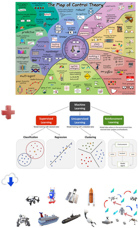
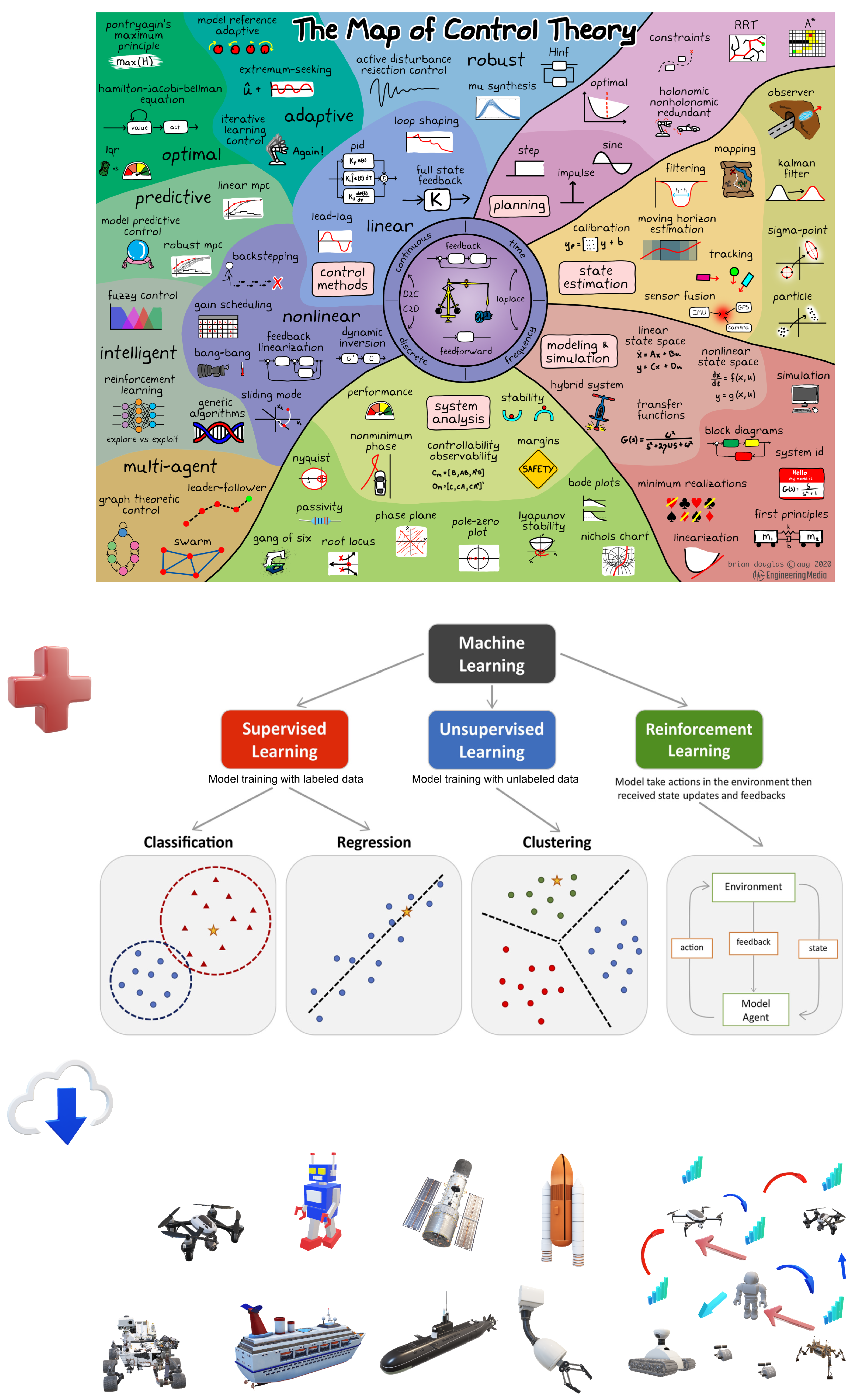
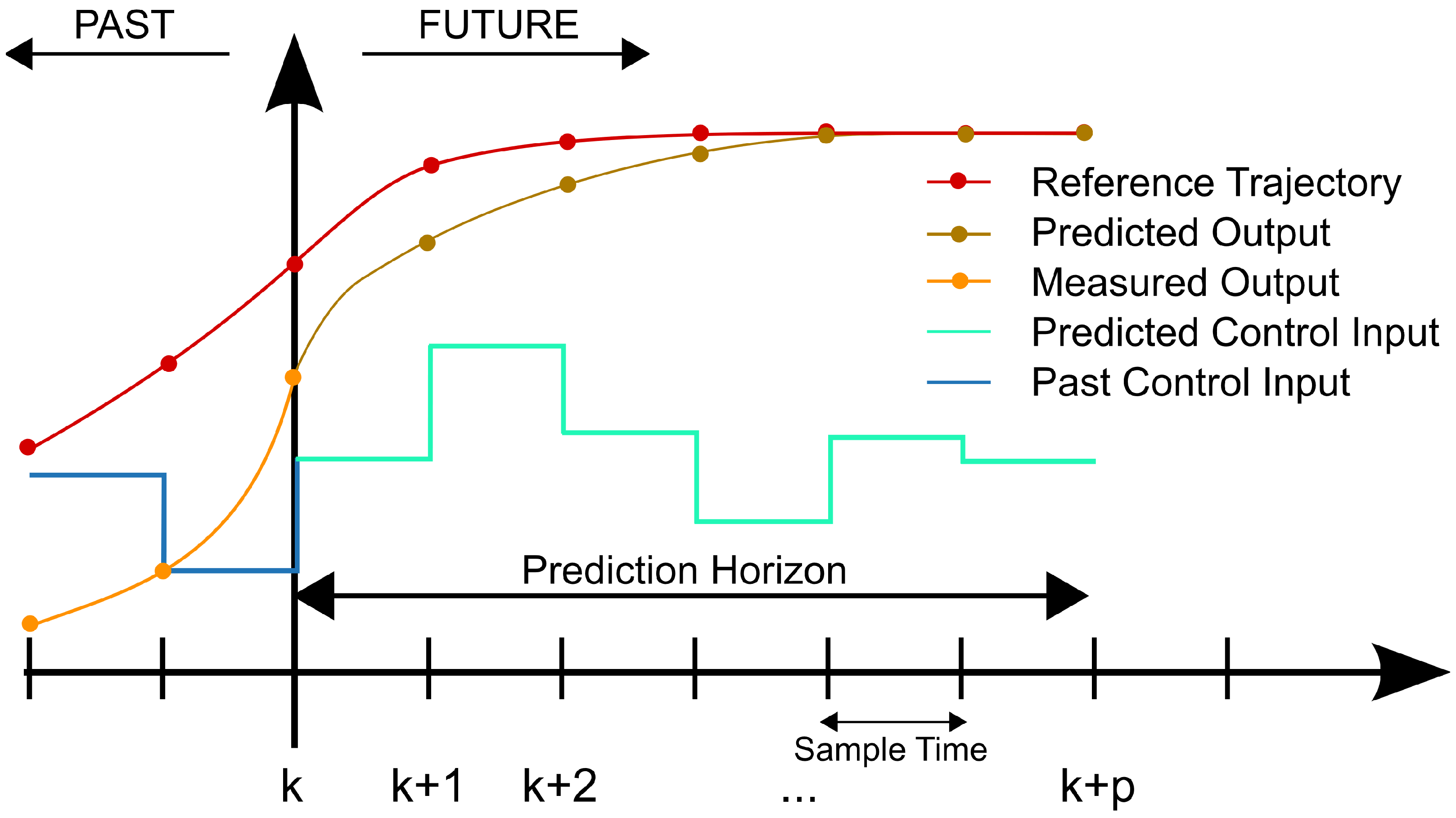
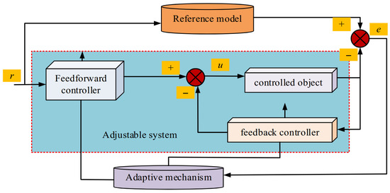
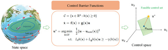
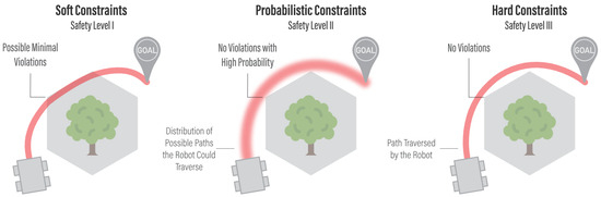
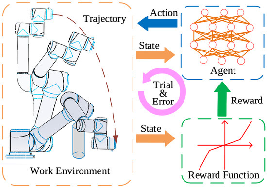
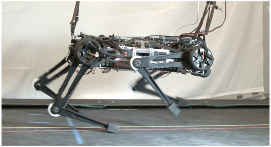
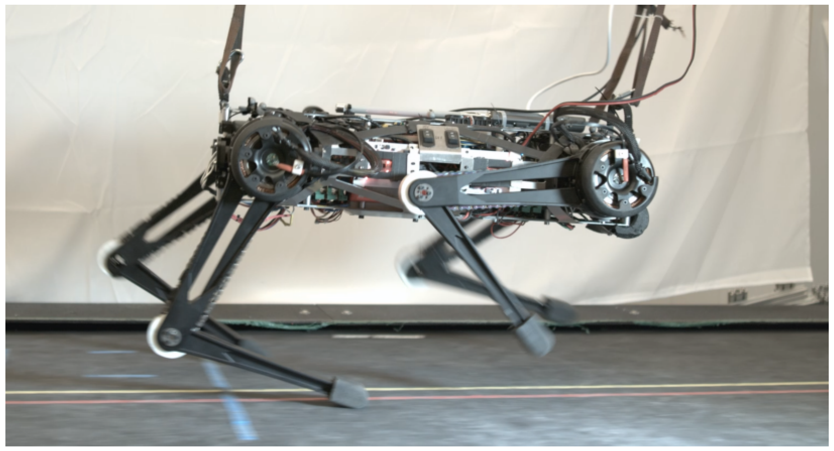
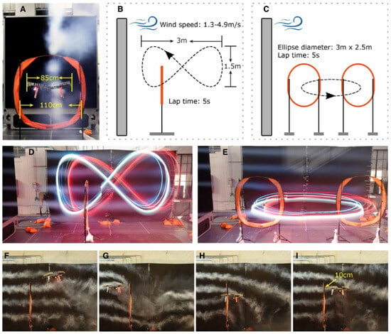
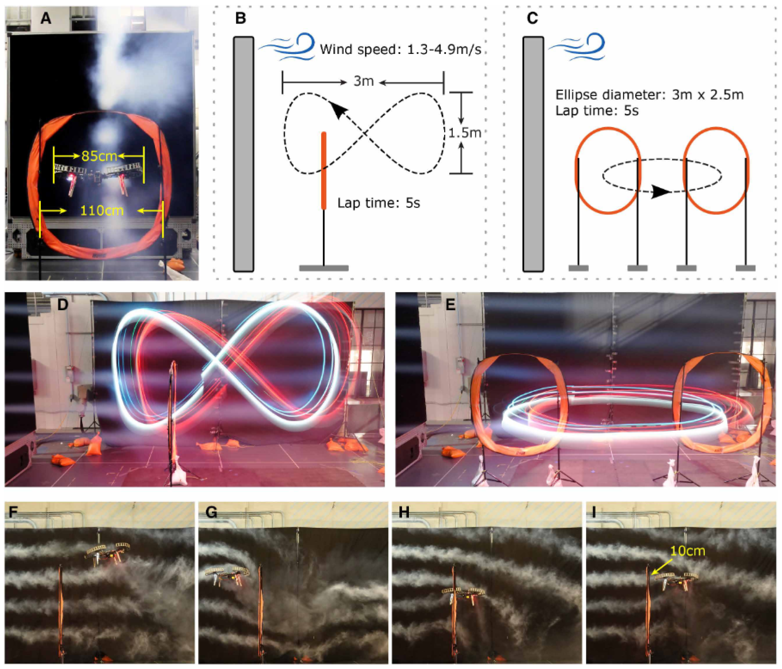
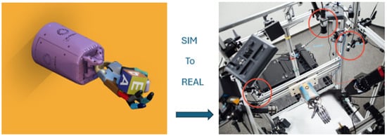
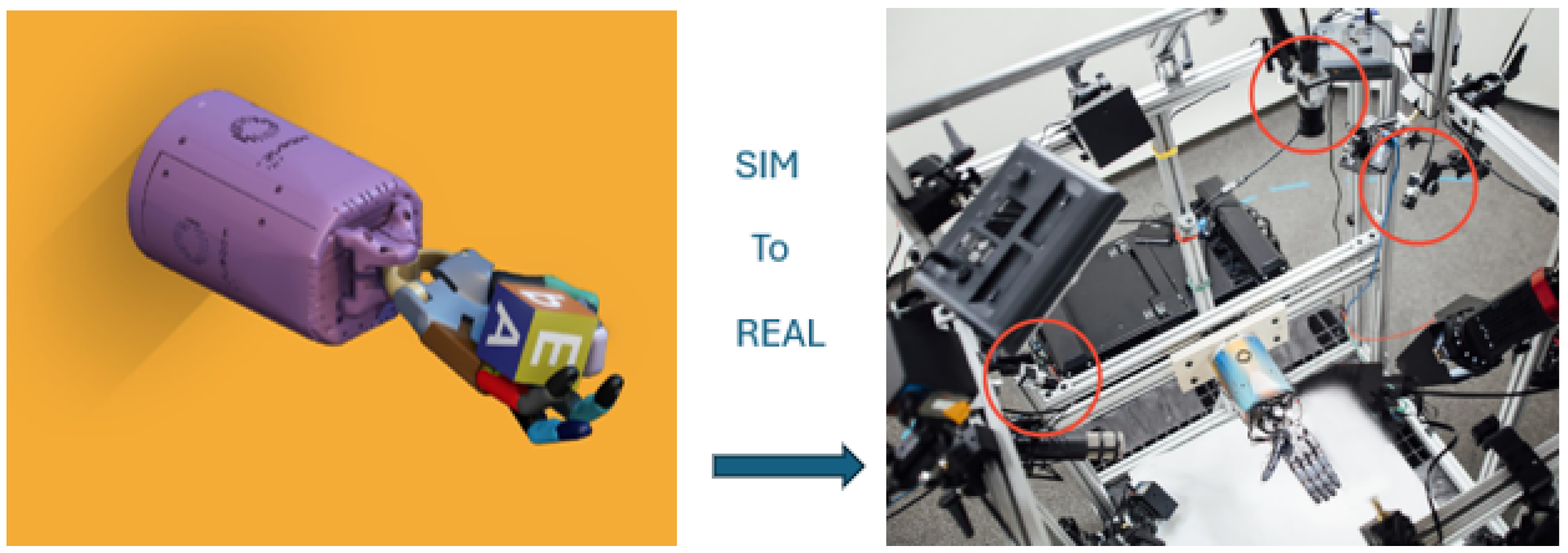
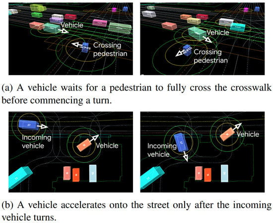
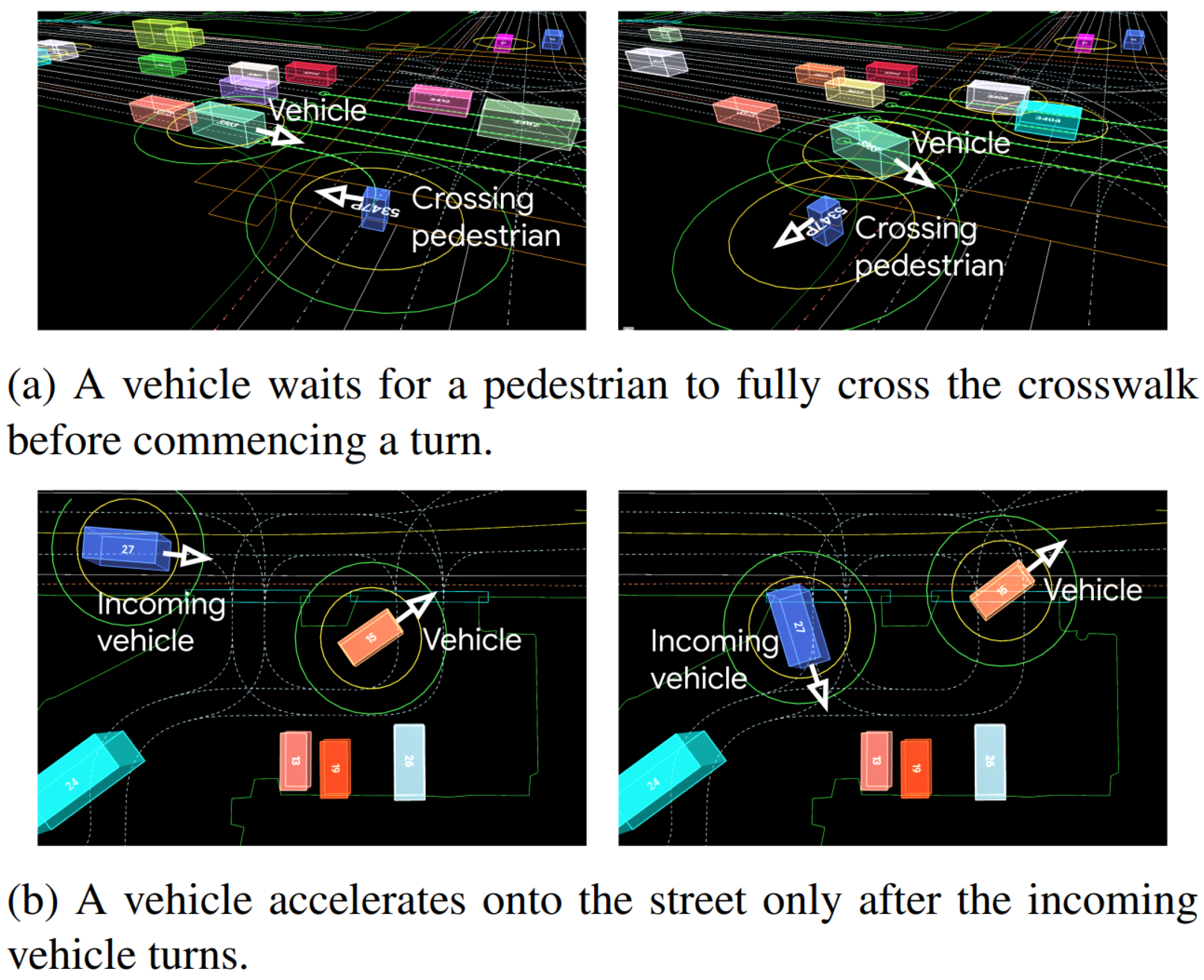
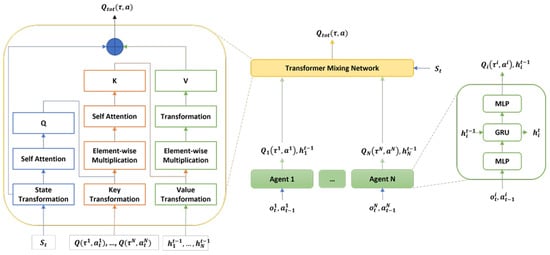
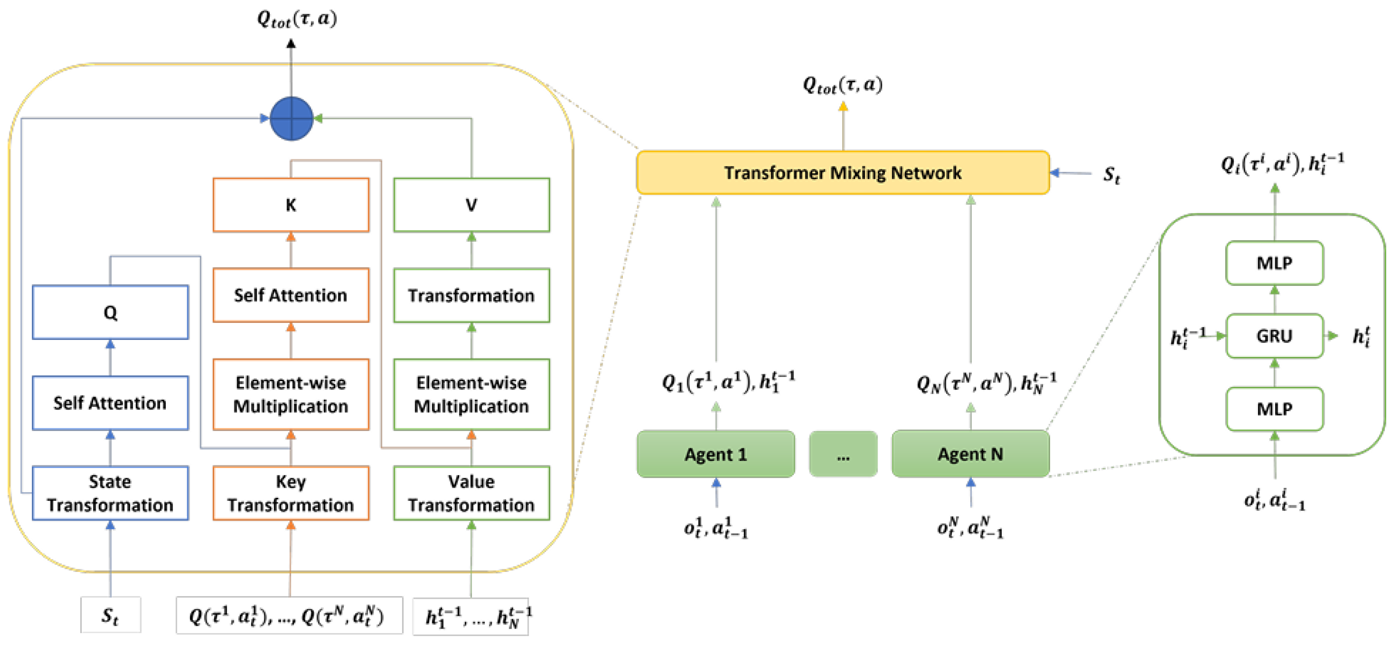


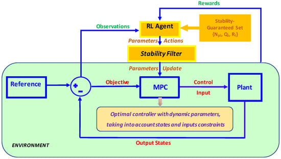
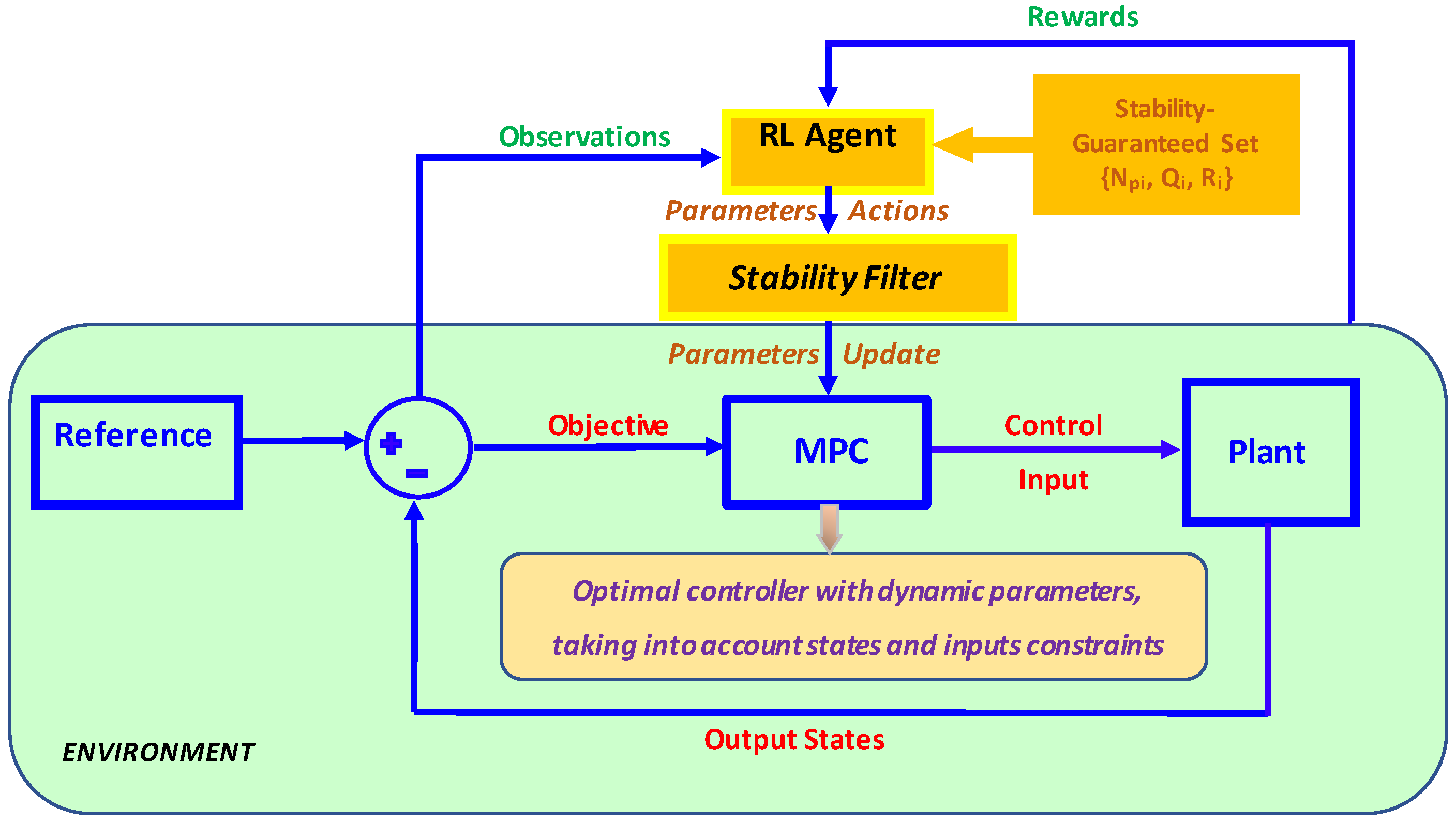
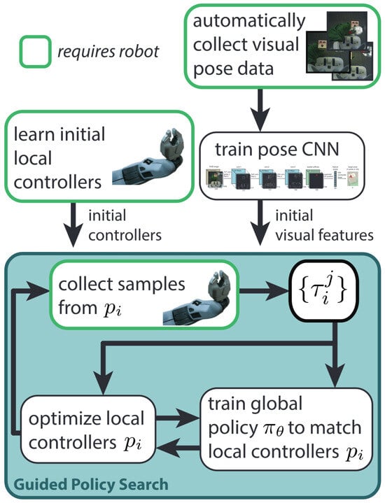
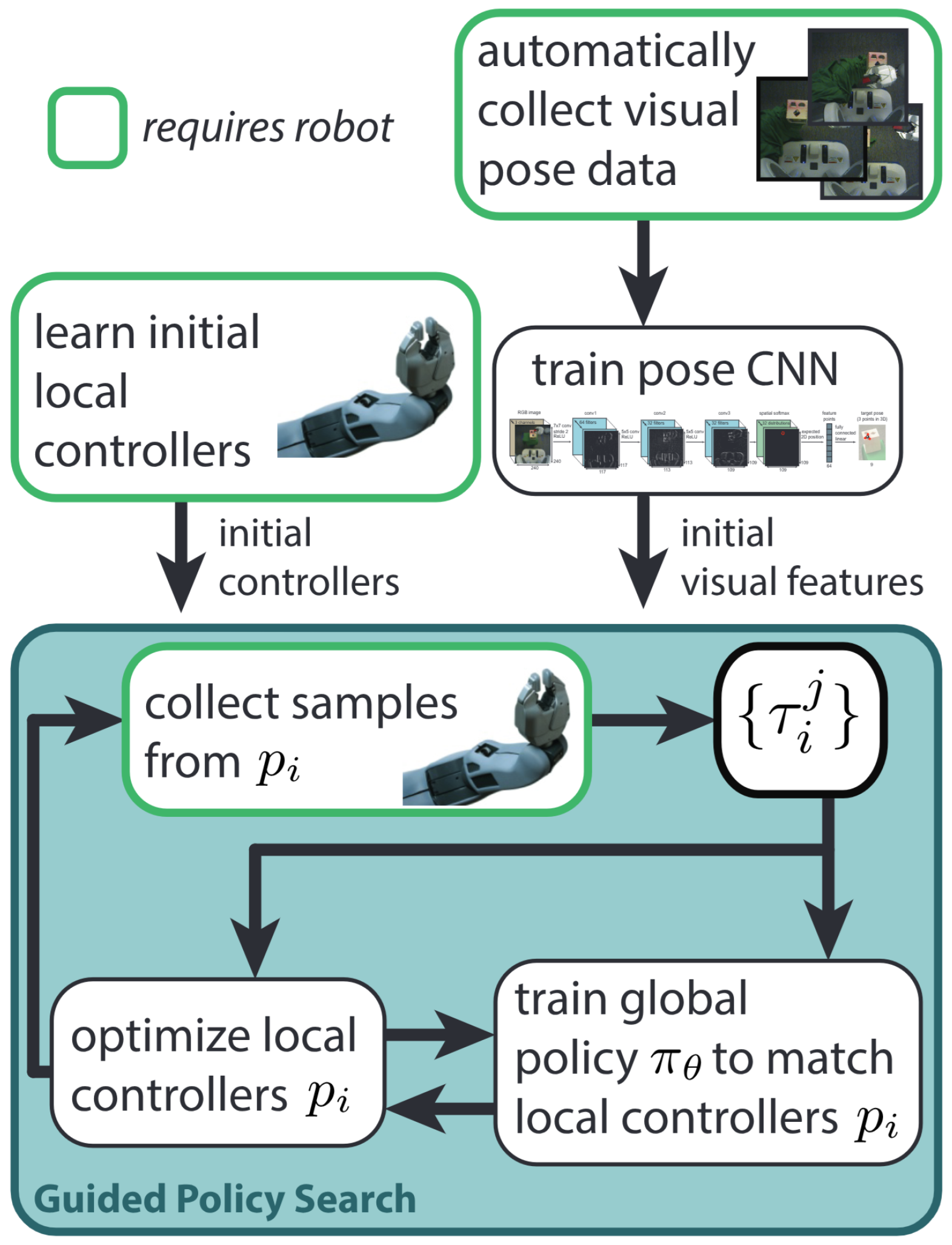
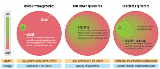
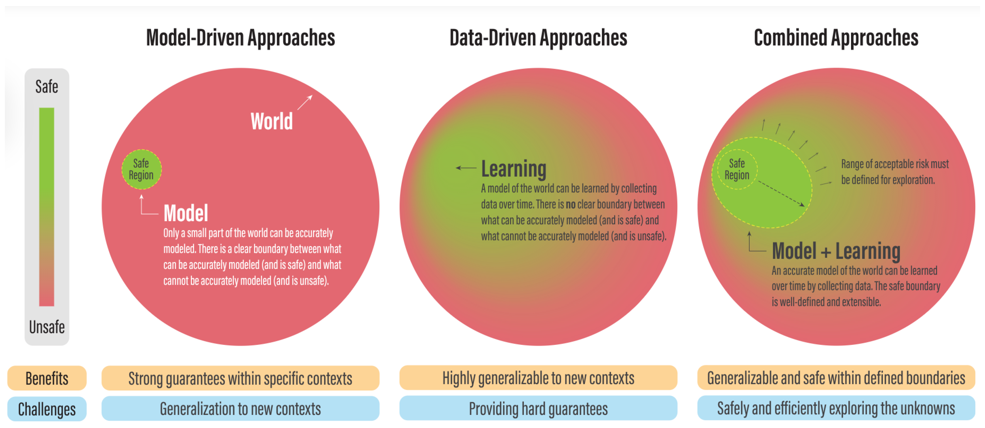
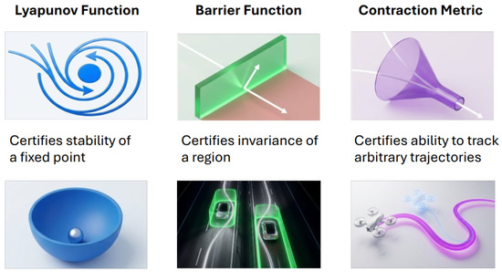
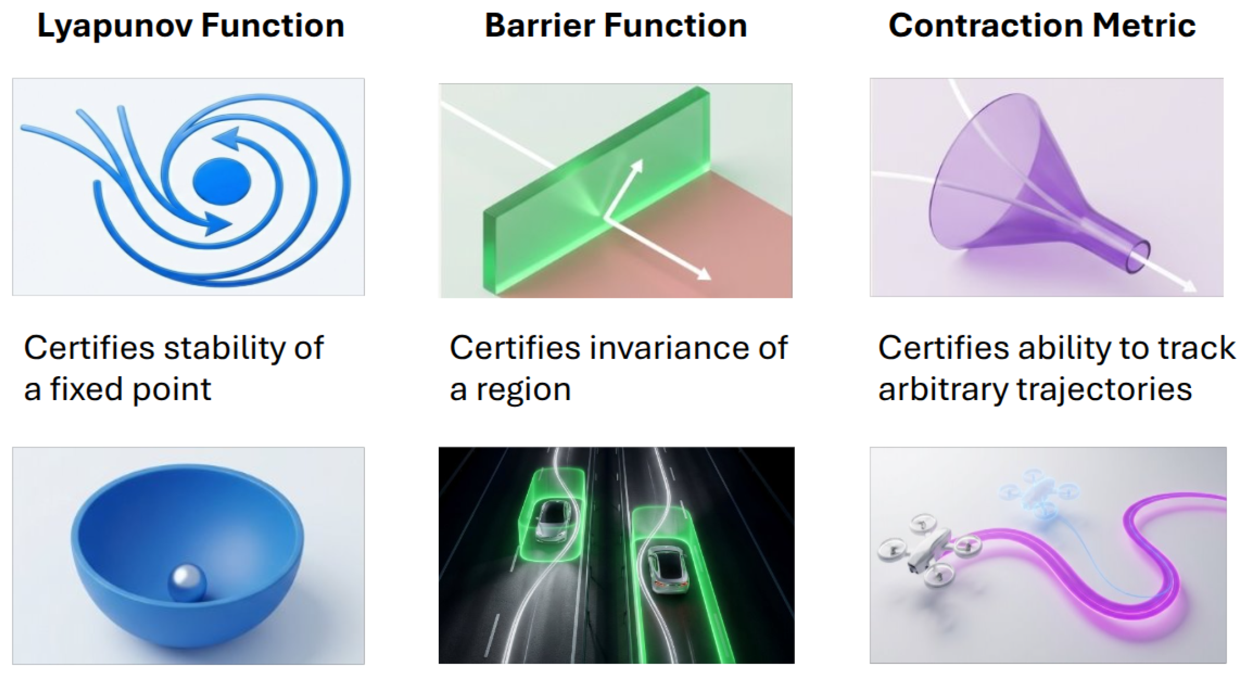
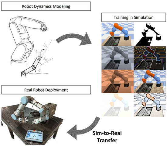
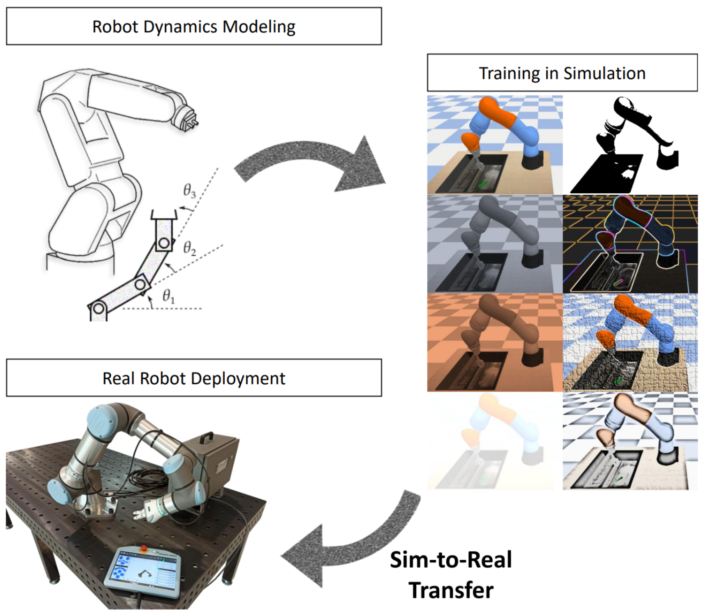
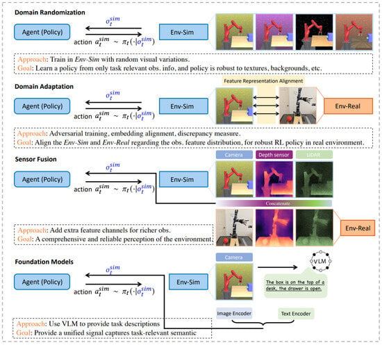
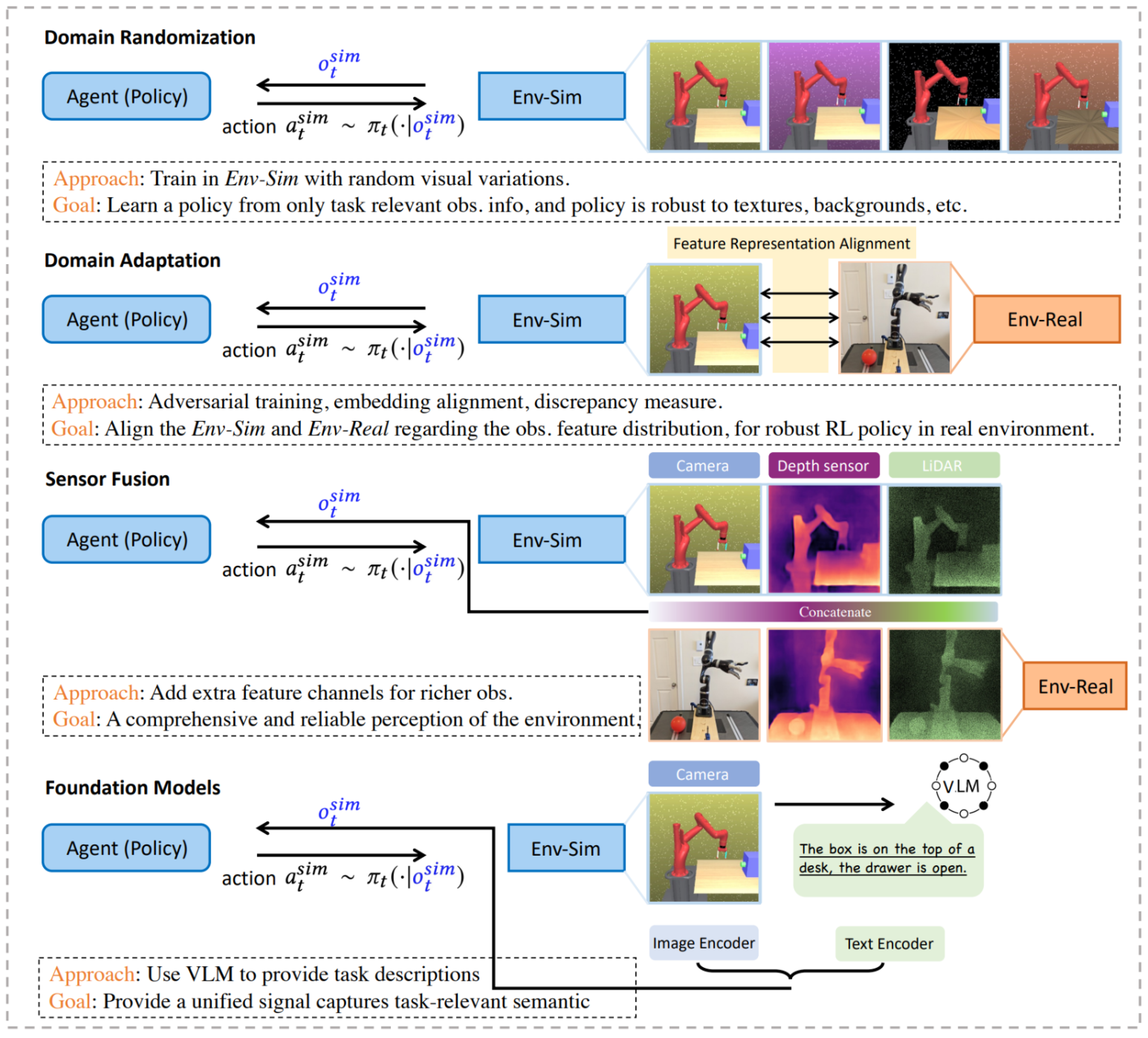
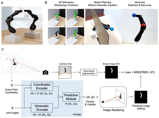
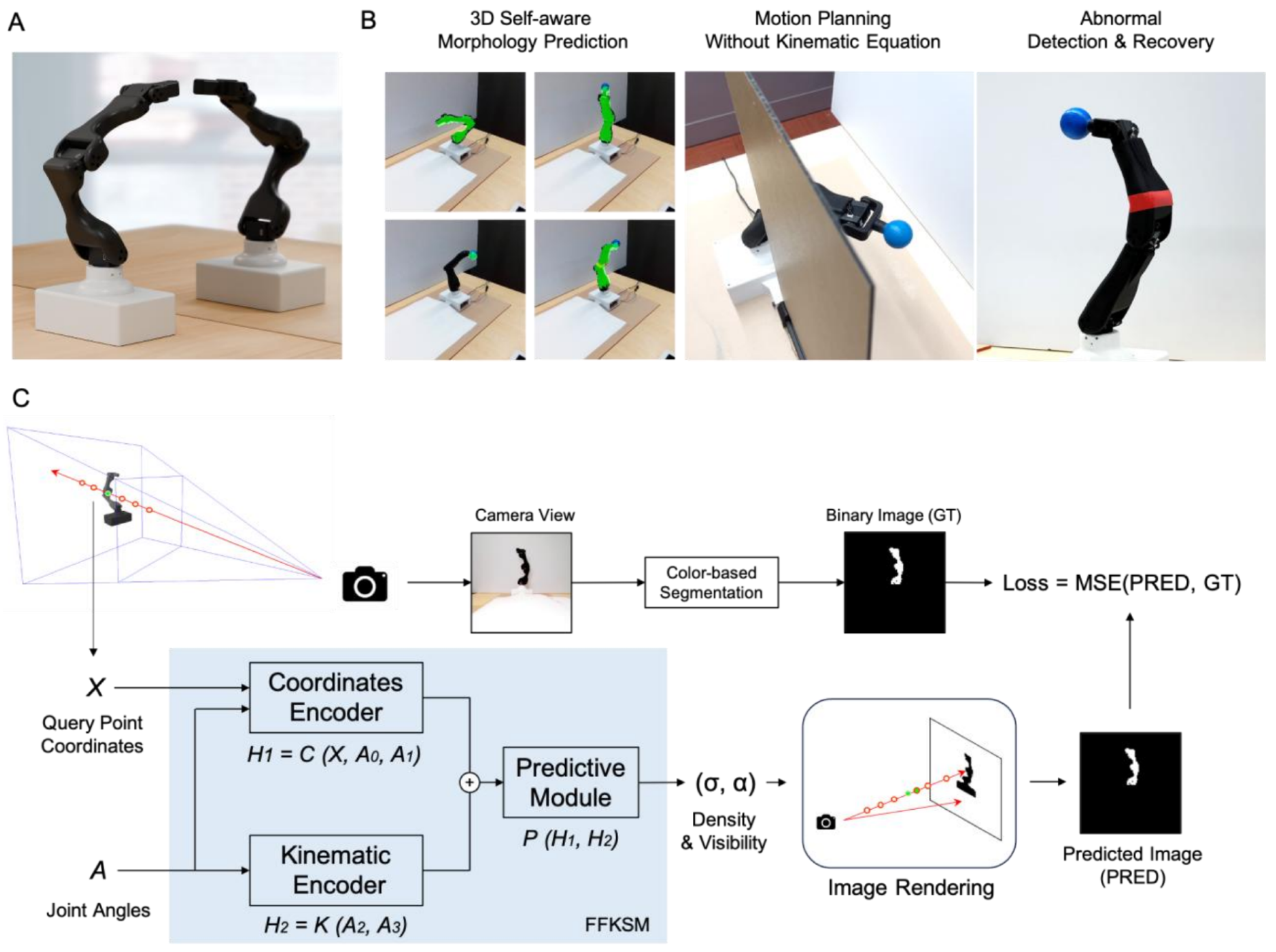
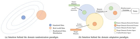
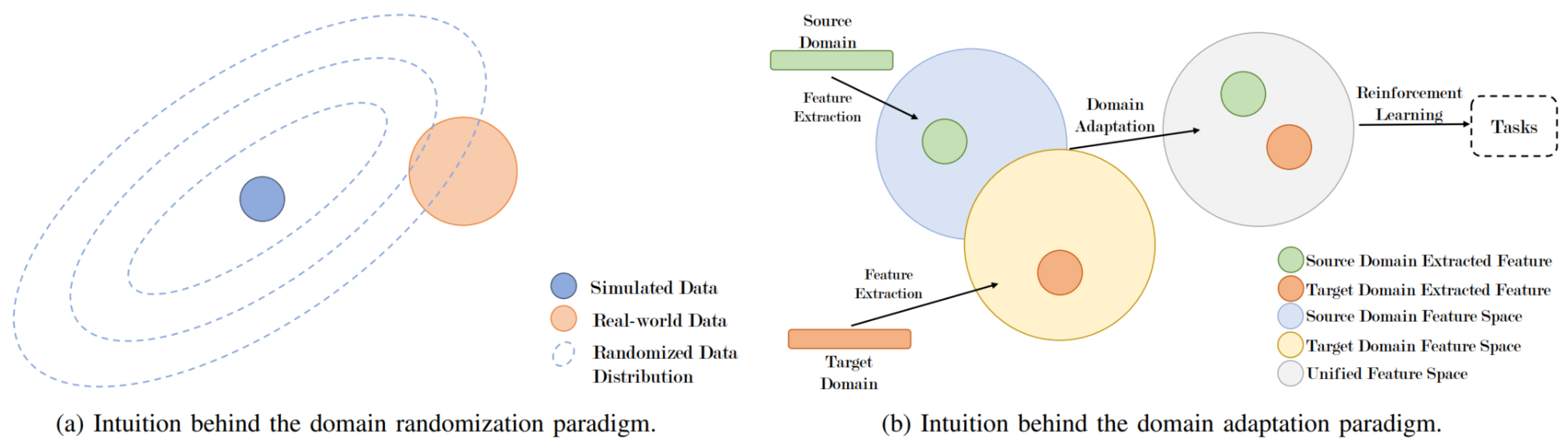
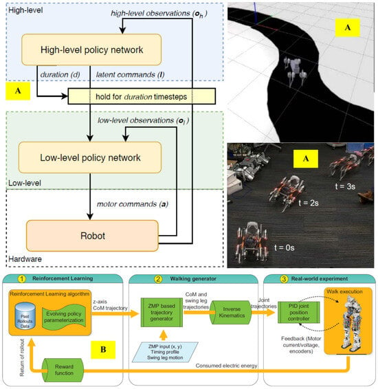
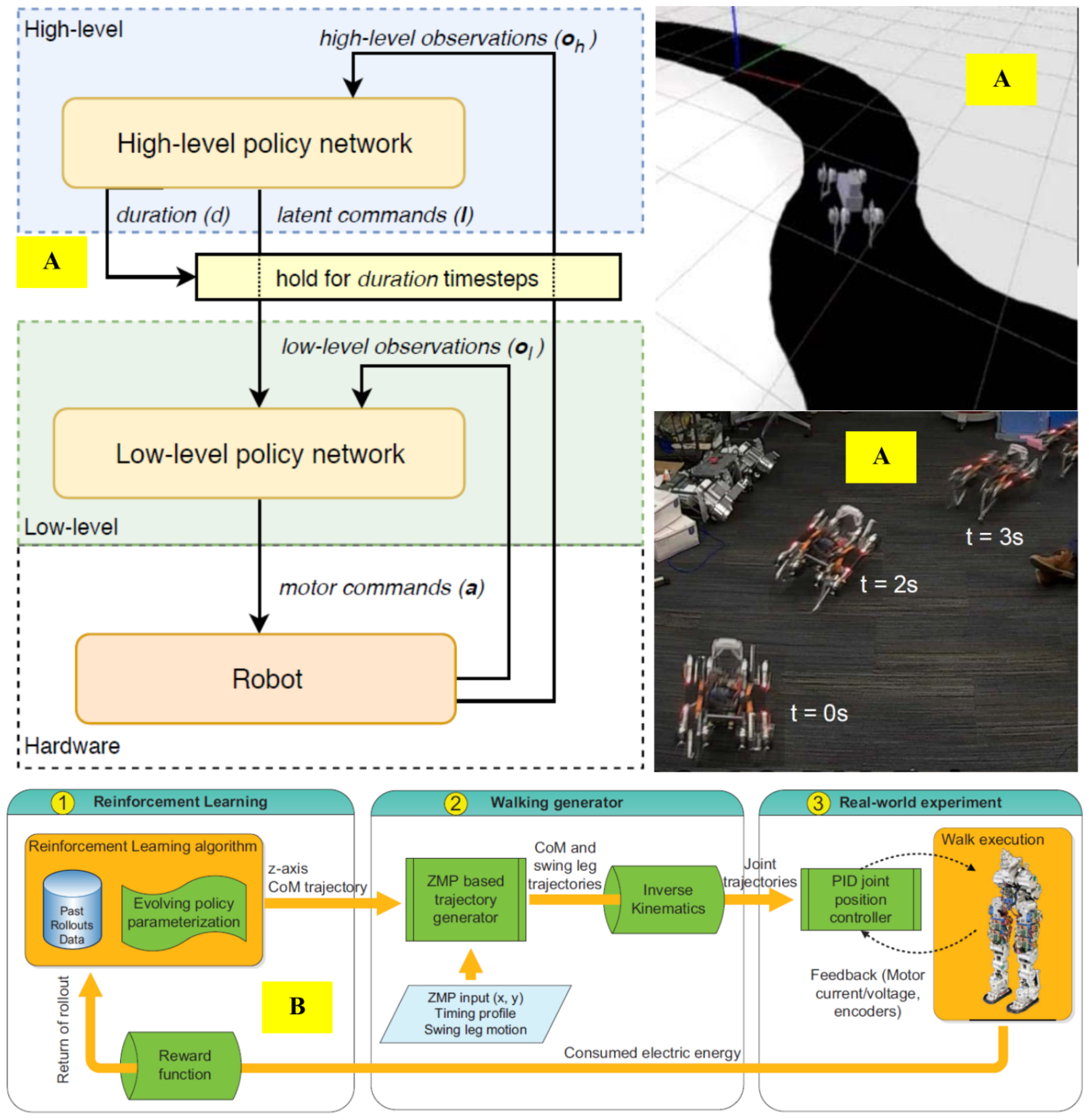

Disclaimer/Publisher’s Note: The statements, opinions and data contained in all publications are solely those of the individual author(s) and contributor(s) and not of MDPI and/or the editor(s). MDPI and/or the editor(s) disclaim responsibility for any injury to people or property resulting from any ideas, methods, instructions or products referred to in the content. |
© 2026 by the authors. Licensee MDPI, Basel, Switzerland. This article is an open access article distributed under the terms and conditions of the Creative Commons Attribution (CC BY) license.