


Abstract
Space robots operate in unconventional environments, which places specific demands on their mechanical, actuation, and control systems. They need to address a variety of challenges in future space exploitation and exploration, such as in-orbit deployment, active debris removal, or servicing operations. Using robots for such applications presents a unique challenge, as a high level of autonomy is required, and the manipulator’s motion affects the position and orientation of the spacecraft. The article presents basic theoretical statements regarding redundancy in space robotics. Various methods for overcoming difficulties in designing, using, and controlling a space robot are considered. Specialized control algorithms based on the null space of the Jacobian matrix and zero reaction maneuvers (ZRMs) are discussed. The review is limited to space robots with one or more arms and does not include mobile and humanoid robots. Furthermore, the primary motion planning algorithms for these systems are evaluated. Redundant space robots are categorized based on their degrees of freedom, number of arms, operational efficiency, primary objectives, and application areas and the most commonly used algorithms for planning movements. The advantages and disadvantages of both redundant and hyper-redundant space robots are analyzed. The objective of this review is to provide a comprehensive overview of the current state and prospects for the development of redundant robots for operation in space conditions.
1. Introduction
Space robots have a history of over 40 years. They have several main tasks, such as in-orbit deployment, active debris removal, or servicing operations. In 1981, the SRMS manipulator, also known as Canadaarm1, was used for deploying payloads, constructing the ISS, and assisting astronauts in repairing the Hubble Space Telescope [1]. The German manipulator ROTEX, which was launched in 1993, verified ground teleoperation technology for the first time and was used for servicing operations, such as assembling mechanical truss structures, connecting and disconnecting electrical plugs, and grasping free-floating objects. Regarding active debris removal, the technology was tested in 2016 by the Chinese robot AL-1 [1].
Redundancy in robotics can be viewed as a system with additional degrees of freedom (DOFs) that are not needed for the primary tasks in a well-organized environment. The tasks performed in orbit require the space robot to operate in an unstructured dynamic environment, where the trajectory of the end effector and the avoidance of obstacles must be simultaneously guaranteed, while its movements should not affect the motion of the space station [2,3]. This requires the use of specialized robots with a large number of degrees of freedom, which in turn require specific control algorithms. The presence of additional degrees of freedom allows the space manipulator systems (SMSs) [2] to tackle unexpected tasks, as it is impossible to determine all conditions in the space environment. The existing scientific literature covers the overall Guidance, Navigation, and Control (GNC) of the mission [4], the dynamics of free-floating SMSs in space, and robotic target acquisition tasks in orbit [2], as well as on-orbit servicing technologies [5]. In ref. [3], a literature review is conducted that covers multi-arm redundancy, but experiments with single-arm redundant robots are not included. The overview of the topic of using redundant robots in space is necessary, because the redundant degrees of freedom are used to mitigate dynamic coupling and minimize reaction forces/moments at the base. Dynamic coupling is the mutual influence between the motion of the manipulator and the motion of the spacecraft in a free-floating system [2], arising from the conservation of linear and angular momentum, and is a fundamental task for the control of these systems [3]. This reaction is undesirable, as it can disrupt orientation, communication, or mission safety.
The first redundant robots used in space missions were the Canadarm2, launched in 2001, and Dextre (Special Purpose Dexterous Manipulator, 2008), initiated by the German Aerospace Center (DLR), used on the ISS [1]. Each of these has seven DOFs. The first dual-arm robot used in space is Engineering Test Satellite VII (ETS-VII), launched by the Japanese Space Agency (NASDA, now JAXA) on 28 November 1997. While the primary “main” arm was a large 2 m, six-DOF manipulator, the satellite also carried a secondary, smaller robotic system during its mission to test complex interactions. The first integrated dual-arm system in space, designed to work together like a human torso, is Dextre in 2008 [1]. Redundant robots operating in environments with obstacles require specific motion planning algorithms, such as Rapidly Exploring Random Trees (RRT) and Virtual/Artificial Potential Fields (APF), which were originally developed for Earth-based robots. Historically, in space missions, the RRT algorithm was first seriously considered for autonomous navigation in preparation for complex missions such as Mars 2020 (Perseverance). Modern concepts for space debris capture or satellite servicing use improved versions, such as RRT*, to optimize fuel and energy consumption during zero-gravity travel [6,7]. The first significant application of the APF algorithm in orbit was associated with the Japanese Engineering Test Satellite VII mission, launched on November 28, 1997. ETS-VII demonstrated, for the first time, that APF could successfully handle the dynamics of a free-flying robot, where the movement of the arm affects the orientation of the entire satellite. The algorithm was implemented in the motion planning systems of Dextre and Canadarm2 to prevent collisions with the complex structure of the station during complex maneuvers.
The purpose of this article is to examine the use of redundancy for planning trajectories and additional tasks through control in the null space of the Jacobian matrix; the use of zero reaction maneuvers (ZRMs) [5]; presentation of the basic equations of free-floating SMSs and comparison of the control algorithms used; and systematic analysis of the choice of degrees of freedom and redundancy.
These goals are reflected in the following research questions:
Q1: What are the types of redundant space robots according to the degrees of freedom, number of arms, and manipulator efficiency?
Q2: What is the application of redundant robots in outer space and on the space station?
Q3: What are the main goals for using redundancy in space robots?
Q4: What are the most commonly used algorithms for planning the movement of redundant robots in space?
Another objective of this review is to analyze the results of the above research questions and to discuss the advantages and disadvantages of redundant and hyper-redundant space robots.
2. Theoretical Bases
2.1. Redundancy in Robotics
The basic meaning of the word “redundancy” is a function that is no longer necessary due to the fact that it is duplicated and performed by other elements or in some other similar way. This definition does not accurately reflect the meaning that is understood in robotics. When additional degrees of freedom are used, it is obvious that the design foresees a secondary objective and does not add complexity for the sake of complexity itself. The additional capabilities are not redundant in practice but are used for non-traditional purposes and/or secondary tasks. In the scientific literature, such non-traditional purposes are the simultaneous execution of tasks [8], the capture of objects with uncontrollable motion such as a tumbling target under uncertain parameters [5,8,9], simultaneous control of the gripper position and spacecraft orientation [5], and collision avoidance using free degrees of freedom [10].
If we consider the highest level of redundancy relevant to robots, it can be categorized as: sensory (or information), control, and mechanical redundancy. Sensor redundancy occurs when there are more sensors than theoretically necessary, usually when high reliability is required. Control systems, such as hardware and algorithms, can also be duplicated. Parallel calculations are performed, multiple processors and power modules are used, etc. Mechanical redundancy, in turn, can be divided into kinematic, dynamic, and actuator. Actuator redundancy deals with the issues of driving a single joint by two or more motors. Although sensory, control, and actuator redundancies are important for space manipulators, they are not considered in this article, because they do not have a direct impact on the planning of robot movements in a space environment. Dynamic redundancy describes the presence of redundant degrees of freedom arising not from the kinematic structure but from dynamic dependencies in free-floating and flexible robotic systems. In [11], redundant dynamicDOFsFs arising from a free-floating base (with six DOF) and flexible structures with “n” DOF are used.
In this work, we focus on kinematic redundancy. The definitions are very similar, but the most general one is given in [12,13]. This definition provides a simple method for describing different potential cases of robots related to the dimensions of the space of the end effector and the task space. Later, this definition was used with some modifications in many articles, and in 2020, it was systematized in [14]. The variables that define the position and orientation of the end effector of the robot with respect to a fixed coordinate system are collected in a single vector. Here, this vector is denoted by x (m × 1). Thus, the set of all possible vectors x forms an extended workspace W of the robot, which takes into account the position and orientation of the end effector. The variables that define the configuration (the mutual arrangement of the links) of the robot are organized in another vector. This vector is denoted by q (it has dimension n × 1). The set of all possible configurations defines the configuration space C. Taking into account these considerations from [13,14], the following definitions are introduced:
Definition 1.
A robot is considered kinematically redundant if the dimension m of its extended workspace W is lower than the dimension n of its configuration space C, i.e.,
Sometimes such a mechanical structure is also called inherently kinematically redundant, since this property is built into the robot and does not depend on the task to be performed. From this definition, it is obvious that a spatial robot is kinematically redundant if , and a planar manipulator is kinematically redundant if .
Definition 2.
The difference r between the dimension n of the space of controllable generalized coordinates C and the dimension m of the extended workspace W is called the degree of redundancy (DoR).
When n = m, this is a non-redundant robot. It can be noted that m ≤ 6 describes the degrees of freedom of the end effector, while n coincides with the number of motors of the robot and describes the number of independently controllable parameters.
Definition 3.
A robot is considered kinematically redundant with respect to its assigned task if the dimension t of the task space T is lower than the dimension n of the configuration space C for the execution of T, i.e.,
A consequence of this definition is that all inherently kinematically redundant robots are also redundant for the tasks, but the opposite is not necessarily true. For example: if the end effector has to move along a plane curve, then t = 2. In case it is necessary to follow a spatial trajectory (without caring about the orientation), t = 3. For a welding robot, it is necessary for the end effector to have fiveDOFsFs (i.e., t = 5), three DOF for following a spatial trajectory, and only two for changing the orientation, because twisting around the tool axis is not necessary.
Definition 4.
The degree of redundancy of the task is given by analogy with (2) from the equation:
Thus, a standard non-redundant robot, in some cases when performing a specific task, can be considered redundant with respect to it. There are some situations in which n < t (respectively, n < m) does not make sense, because this means that the degrees of freedom of the robot are not enough to perform the task. There are robots with a large redundancy. By analogy with living nature, they are often called snake-type or proboscis-type robots. For them, the size of the configuration space is much larger than the degrees of freedom of the end effector n ≫ m and are known as hyper-redundant robots.
It should be noted that the degrees of freedom n for a robot (respectively, redundancy r) can change in different regions of the configuration space C if there are obstacles in it and also in singular configurations.
2.2. Kinematics of Redundant Robots
The position and orientation x of the robot’s end effector in space at a certain moment t of time depends on the configuration of the joints q. Mathematically, this is expressed as a functional relationship between the vectors x and q:
This relationship is known as forward kinematics. In redundant robots, this is a nonlinear system of m equations with n unknowns such that n > m.
The forward kinematics problem finds a unique solution for the system (6). Problems arise when we try to solve the inverse kinematics problem: find a vector q(t), which performs the task (at any time t). When the robot is redundant, there are infinitely many solutions (even for x(t) = constant). Figure 1 gives an example of a planar serial redundant robot with four DOFs. When the lengths of the robot’s links and the configuration of the joints defined by the vector of joint angles are known, after solving the forward problem, a unique solution is reached (at a certain time t) for the position and orientation of the end effector . In the inverse problem, however, for a certain position and orientation of , many solutions can infinitely be found (Figure 1b).
Figure 1.
Planar redundant robot. (a) A unique solution to the forward problem and (b) infinitely many solutions to the inverse kinematics problem.
Solutions to the inverse problem are mainly sought at the differential level [12,14,15,16]. The linear and angular components of the velocity of the end effector can be related to the velocity of the joints. This relationship is expressed mathematically as:
where contains the linear and angular velocity components of the actuator, is the joint velocity, and is the (m × n) Jacobian matrix of the robot. Equation (7) is known as the differential kinematics of the robot. Equation (7) has an interesting mathematical interpretation. All possible joint velocities, , form an n–dimensional space, which is a subset of . The number of columns, n, corresponds to the joint angles, number of DOFs, and the number of independently controlled motors of the robot. The velocities are limited by the capabilities of the motors. Also, all possible velocity vectors of the end effector form an m-dimensional mathematical space, which is a subset of . Here, is the set of real numbers. With these refinements, for any fixed configuration q, the Jacobian matrix J(q) can be interpreted as a linear transformation that converts vectors from the space into the space .
Like any other linear transformation, the input space of the Jacobian matrix has two important related subspaces. These two subspaces are called the range (or column space of the matrix) and the null space (kernel of the matrix). The range of the Jacobian matrix is the subspace of that is spanned by the transformation. Physically, these are the joint velocities that are mechanically possible to be generated by the robot actuators. The range is defined mathematically by Formula (7):
2.3. Null Space of the Jacobian Matrix
The null space of the Jacobian matrix is a subset of the input space such that it maps the null vector into the output space by means of the Jacobian matrix [12,16]. Physically, these are possible joint velocities that do not generate any velocity in the end effector. The null space of the Jacobian matrix is denoted by and can be defined mathematically by:
The existence of a null space, defined by Formula (9), for the Jacobian matrix is an important mathematical basis for redundant manipulators. Physically, Formula (9) implies that the velocities, , chosen from the null space do not generate any velocity in the end effector, i.e.,
The presence of additional DOFs, beyond those strictly necessary for the task, provides the flexibility to avoid obstacles, constraints, and singular configurations. This flexibility is due to the existence of countless joint configurations for the same pose of the end effector (Figure 1). As a result, there is joint motion that can be propagated in the null space of the Jacobian robot without affecting the position and orientation of the end effector. This phenomenon, commonly called “Self-motion”, was introduced by Nakamura in 1991 [15].
Although the velocities do not generate motion in the end effector, they do generate internal joint motions. Therefore, these velocities can be used to satisfy other requirements of the redundant manipulator, for example, to avoid obstacles from the joints while the end effector performs its primary task.
The dimension of the null space from which can be chosen depends on the rank of the Jacobian matrix [12,14]. If the Jacobian has full rank for a given configuration q, then the dimension of the null space is equal to the degree of redundancy r. If the Jacobian matrix has rank , the dimension of is equal to . Since the choice of velocities that belong to the null space is not unique, there are several ways in which the desired basic task can be achieved. Useful additional constraints can be defined wisely. There are two approaches to defining additional constraints: global and local. Global approaches achieve optimal behavior along the entire trajectory, but their computational complexity makes them unsuitable for real-time robot control applications. In real-world robot applications, the desired trajectory of the end effector is defined as the primary task. However, for controlling the manipulator, the trajectory in the joint coordinate space is required. In the first step for redundant robots, the solution is done at the velocity level, i.e., the desired joint velocities are calculated that generate the desired velocity for the end effector. This is known as the reduction resolution at the velocity level. Due to kinematic redundancy, there are always more unknown joint velocities than equations. Mathematical methods can be categorized into two types: exact and approximate solutions. The pseudo-inverse method and Jacobian matrix complementation are two methods for exact solution.
2.4. Pseudo-Inverse Method in Redundant Robots
One of the methods used to obtain the exact solution is to find the pseudo-inverse of the matrix , denoted by [12,16], and used as:
where the index p indicates that this is a primary solution of Equation (7). This solution can later be improved by adding other solutions from the null space of the Jacobian . If has full rank, then its pseudo-inverse is:
It is known as the Moore–Penrose generalized inverse. The pseudo-inverse method can provide a solution regardless of any imbalance in the number of equations and unknowns in Equation (7). However, Equation (11) only provides a primary solution that is not in the null space of the Jacobian . This means that the excess of the manipulator, which has additional DOFs, cannot be used for any useful purpose that can be defined as an auxiliary task by the user. This problem can be solved by adding a joint velocity vector that belongs to the null space of the Jacobian matrix .
The new joint velocity still satisfies Equation (7). The vector can be chosen as:
where v is an arbitrary n-dimensional vector that will be reasonably chosen to satisfy the desired secondary task. I is a singular matrix. This desired auxiliary task can be the minimization of torque and acceleration, singularity avoidance, or obstacle avoidance. To achieve any of these additional tasks, a cost function is defined whose optimal value would provide the desired secondary task. Then, the arbitrary vector v can be chosen such that the solution given by Equation (14) converges to the optimal value of the cost function. A problem with the solutions presented by Equation (11) is that they can lead to configurations for the manipulator in which the Jacobian matrix does not have full rank. In these singular configurations, the robot end-effector cannot generate velocity components in certain directions, which is undesirable. Near the singular position, very large joint angular velocities are required to generate end effector velocities in certain directions.
2.5. Improved Jacobian Method
In the improved Jacobian method [12,16], for a redundant manipulator with a redundancy of r = n − m, secondary tasks are defined. These auxiliary tasks, which are functions of the joint variables q, are organized in an r × 1 vector represented by z. Since the secondary task z is a function of the joint variables vector q, an r × n Jacobian matrix , known as the Jacobian of the additional task, can be defined in a way that relates their rate of change as:
Equation (15) adds r equations to the forward kinematic equations of (7), resulting in a total number of equations n. Since there are n unknown joint velocities in , by defining the derivatives of the additional problem z, the number of equations and unknowns will balance. This is expressed by defining an extended vector of problems as:
The enlarged problem, with respect to the joint velocity vector, is:
where is the (n × n) augmented Jacobian matrix, and and are (m × n) and (r × n) Jacobian matrices of the primary and secondary tasks, respectively. Since the augmented Jacobian matrix in Equation (17) is square, the solution for the joint velocities can simply be found using the inverse of . This is a very simple approach, but there are two main drawbacks associated with this method. This method requires the calculation of the inverse of the augmented Jacobian matrix. In order for the inverse of the augmented Jacobian matrix to exist at any time, the secondary tasks must also be defined at any time. In other words, auxiliary tasks, such as obstacle avoidance or joint constraint avoidance, are defined based on some conditions that may not exist at any time and cannot be used as secondary tasks. Another drawback is that additional singularities of the redundant manipulator can be introduced into the kinematics by defining the auxiliary task. This may be due to additional singularities that are a consequence of possible rank deficiencies of the secondary task in certain configurations. Or it may be caused by an undesired conflict between the primary and secondary tasks in certain configurations, in which the rows of and become linearly dependent. This linear dependence, which leads to a singularity in the matrix , depends on the tasks and is difficult to predict.
2.6. Zero Reaction Maneuvers
One important feature that clearly distinguishes space robots from other ground-based robots, such as industrial manipulators, is the presence of a mobile base. This is a system of freely floating bodies. A space-based free-flying vehicle that has one or more robotic arms is a typical example of this group [16], as illustrated schematically in Figure 2a.
Figure 2.
System of a spacecraft and robot. (a) a typical spacecraft with one robotic arm; (b) spacecraft with a micro-macro manipulator arm; (c) spacecraft with flexible manipulator links.
As the robot’s parts move, the position and orientation of the base spacecraft fluctuate due to the robot’s reaction (influence) to it. The kinetic momentum of the system is conserved unless external forces or torques are applied, and the law of conservation of momentum for this system governs the dynamics of the reaction. The coordination of movements or isolation between the base and the robot, as well as the dynamics of the system, is key to advanced motion control. The reaction null space (RNS)-based reactionless manipulation is used to capture a rotational target by using the momentum conservation law [10].
- Macro–micro manipulator systems.
A robotic system that consists of a relatively small arm (micro-arm) for fine manipulation mounted on a relatively large arm (macro-arm) for coarse positioning is called a macro–micro manipulator system. The concept of the so-called macro–micro manipulator system is introduced by Sharon and Hardt [17]. A small, high-speed manipulator is mounted at the end of a larger one, and the former is controlled to compensate for the inaccuracy and vibrations due to the latter. The SSRMS (Canadarm2) and SPDM (Dextre) systems, as well as the JEMRMS on the Japanese ISS module, are good examples of such systems. Here, the connecting interface at the end point of the macro-arm or the root of the micro-arm is modeled as a main body (Figure 2b). A free-flying space robot can be considered in this group when its main body is actively controlled by actuators that produce external forces and moments, such as gas jet engines. In this case, these executive mechanisms can be modeled as a virtual macro-arm [17].
- Systems with flexible manipulators.
If the macro-arm behaves as a passive flexible (elastic) structure in the macro–micro robot, the system is considered a manipulator with flexible links (Figure 2c). Such a situation can be observed in the operation of the ISS. Here the problem is that the main body (the root of the micro-arm or the end of the macro-arm, according to the above definition) is subjected to vibrations, which will be excited by the response of the micro-arm.
- Equations of free-floating manipulation systems.
The equations of a freely floating system with one or more robots mounted on a base spacecraft are considered in [16]. It is assumed that the main body is floating in inertial space without any external forces or moments. External forces/moments are applied to the robot’s end effector. The following equations of motion are derived for such a system:
, , and are the inertial matrices, respectively, for the main body of the spacecraft; the robot and the connection between the main body and the robot, respectively; and and are the nonlinear Coriolis forces and centrifugal forces, respectively. The kinematic relationship between , and is expressed using Jacobian matrices for the robot and the base as:
where
- —vector that defines the position and orientation of the base;
- —vector of the robot’s joint angles;
- —sets the position and orientation of the end effector relative to the base;
- —vector of torques at the robot’s joints;
- —the external forces and moments applied to the end effector;
- —the number of joints the robot has.
Using Equation (18), the robot can be controlled according to a given velocity or acceleration law in inertial space. More detailed information can be found in [16].
- Reaction null space and zero reaction maneuverers.
As already mentioned at the beginning of 2.5, the robot’s movement and its interaction with external objects can negatively affect the base spacecraft by changing its trajectory or orientation (Figure 3).
Figure 3.
Influence of robot movements on the base spacecraft.
Therefore, robot motion planning methods that minimize perturbations to the base position have been extensively studied [4,16,18,19]. The reaction null space has been introduced as a tool to determine joint velocities that minimize the reaction exerted on the base [20]. Redundant robots can take advantage of the redundancy in the system and generate trajectories with zero reaction maneuvers on the base [20,21].
The concept of reaction null space is first introduced and mathematically formalized in 1994 by Dr. Kazuya Yoshida of Tohoku University [22]. While the physical flight validation happened in 1999 (on the ETS-VII satellite), the theoretical foundation that allowed robotic arms to move without disturbing their base satellite was published five years earlier.
ZRM is a specific algorithm designed to simulate the effect, caused by an impact, on the support reactions of a freely floating platform. The term “zero reaction maneuvering” was first used and validated in flight in September 1999 during experiments with Engineering Test Satellite VII (ETS-VII), a Japanese space robot [1]. The concept focuses on “reaction-free manipulation”, in which the robotic arm moves along a defined trajectory that results in almost zero perturbation of the position of the base spacecraft.
RNS and ZRM differ from other algorithms in their main goal and implementation method. In those two methods, the main goal is to minimize the reaction at the base, while in the other algorithms the goal is to reach a certain point (or configuration) of the end effector while avoiding obstacles. RNS and ZRM are based on dynamic models, while in other algorithms, various approaches are possible, which include randomly generated configurations, kinematic models, heuristic concepts, etc.
3. Algorithms for Planning Motions of Redundant Robots in Space
There are many and various algorithms for planning robot motions in complex environments. Due to the specifics of redundant robots, which have a large number of DOFs, only some of the algorithms are suitable for them. Full and network methods are not suitable for working in multidimensional spaces due to the high computational complexity. The following methods are suitable for planning motions of redundant robots:
3.1. Sampling Methods
A common sampling method is based on a random or deterministic function for selecting a sample from the configuration space C; a function for estimating whether the sample is in the free space; a function for determining the nearest “previous free space sample”; and a local algorithm to try to connect to or move towards the new sample from the previous sample. This process builds a graph or tree representing possible robot movements. Sampling methods are easy to implement, tend to be probabilistically complete, and can even solve motion planning problems with high degrees of freedom. The solutions tend to be satisfactory rather than optimal, and it can be difficult to characterize the computational complexity. Two main methods are used:
- Probabilistic Roadmap Planner (PRM).
This method is described in [16,23]. PRM uses samples to build a path map in the obstacle-free space before responding to specific queries. For this reason, the method is mainly applicable to kinematic tasks for which there is an exact local algorithm that can find a path (taking into account obstacles) from any configuration to any other configuration (nodes on the map). PRM can be divided into two phases, a learning phase and a query phase. Prior information about obstacles is required, which is why it is used for static environments.
- Rapidly Exploring Random Trees (RRT).
The RRT algorithm searches for collision-free motion from an initial configuration to a target configuration . It is applied to kinematic and dynamic problems [10,11]. The basic RRT algorithm creates a tree with a start—the initial configuration, which gradually grows (by adding new nodes)—configuration as it approaches the target. When the algorithm reaches a point in a predefined target region, it is considered to have reached the goal (Figure 4).
Figure 4.
Rapidly Exploring Random Trees.
RRT is developed by Steven M. LaValle and is described in detail in [23]. There are several variations in the algorithm. In the bidirectional RRT algorithm, two trees are grown: one forward from and one backward from . The algorithm alternates between growing the forward tree and growing the backward tree and often attempts to connect the two trees. The advantage of this approach is that the goal can be reached exactly and not just to a target region. Another advantage is that, in many environments, the two trees are likely to be connected much faster than a single tree built forward to a given goal. Algorithms with two or more trees perform better under complex obstacles. The RRT* algorithm is a variant of RRT that continuously reorders the search tree to ensure that it always encodes the shortest path from to each subsequent node in the tree [23]. The application of RRT for the collision-free trajectory planning of a free-floating space robot is presented in [7]. The tree is constructed in the configuration space, and when a new node is added to the tree, whether the manipulator collides with an obstacle defined in Cartesian space is checked. The joint constraints and the allowable torques that can be applied to the joints are checked. In the presented approach, the dynamics equations take into account the momentum and angular momentum of the system. In this way, it is possible to take into account the torques and forces generated by the satellite control system. In [24,25], a combination of the RRT method is proposed, which reduces the metric sensitivity, with a two-way approach to the tree construction in order to achieve faster convergence of the solution.
3.2. Virtual Potential Fields
Virtual potential methods are inspired by potential energy fields in nature, such as gravitational and magnetic fields. From physics we know that the Potential Field P(q) defines a force τ in configuration space C,
which moves an object from high to low potential. Here, q is the configuration of the robot (Figure 5).
Figure 5.
A robot represented as a point in the configuration space is attracted by a “magnetic” force located at the goal and is repelled by the obstacles.
The idea of Artificial Potential Fields for planning robot motion was first introduced by O. Khatib in 1985 [26] and has been further exploited by a number of scientists [27,28]. These approaches in the literature can be found under different names: “Potential Field Approaches”, “Potential Field Methods”, “Artificial Potential Approaches”, “Virtual Potential Approaches”, “Potential Based Approaches”, or “Potential Field-based Navigation Methods”. An Artificial Potential Field is a scalar function defined at each point of the robot configuration space. In this case, two main issues are important for creating such a function. First, we must avoid collisions with obstacles, and second, we must reach the target configuration from any given initial configuration, if possible. This is one of the few methods for planning robot motions in real time.
A multidimensional function P(q) is defined, the gradient of which is used to calculate the torques τ of the motors driving the robot, forcing it to achieve its goal. Obviously, this Potential Field depends on the target configuration and the geometry of the robot’s environment. The artificial field must reach its maximum values at the obstacles and a global minimum in the target configuration. Using a Potential Field to perform a certain movement means that the robot’s trajectory is not known or calculated in advance. This means that the robot “chooses” its own path to achieve the goal. The disadvantage is local minima in the potential function: the robot can get stuck in local conditions where attractive and repulsive forces cancel the movement, but the robot has not reached the goal.
The Artificial Potential Field method for the trajectory planning of a free-floating space robot is presented in [27,28,29]. The proposed approach takes into account collisions between robot links and obstacles. If the distance to one of the obstacles is less than a certain safe distance, then the trajectory of the end effector obtained by the Potential Field method is modified. In the presented example, a robot with six degrees of freedom, mounted on a free-floating satellite, moves through a rectangular window.
3.3. Nonlinear Optimization
The motion planning problem can be transformed into a nonlinear optimization problem by representing the path or controls in terms of a limited number of design parameters, such as the coefficients of a Fourier polynomial. The problem is to determine the design parameters that minimize the cost function, while satisfying the constraints on the controls, obstacles, and the objective. While these methods can produce near-optimal solutions, they require an initial guess about the solution. Because the objective function and feasible solution space are usually non-convex, the optimization process may remain far from a feasible solution, let alone an optimal solution.
In [30], the optimal control law is solved numerically using the Galerkin procedure combined with a nonlinear optimization algorithm. A data-driven approach to Pareto optimal control of large-scale systems is developed in [31], and reinforcement learning is used to design a control strategy that optimally balances multiple objectives. In [32], a model-free control approach for designing the controller and state observer, which are based on the time delay estimation (TDE) method, is presented. In order to achieve high tracking accuracy and convergence speed, the non-singular fast terminal sliding mode is used, along with the super-twisting algorithm and the TDE method.
3.4. Algorithms Based on Neural Networks NN and Others
Reinforcement Learning and Deep Reinforcement Learning Methods
Motion planning for robots in unstructured dynamic environments with obstacles is an active area of research, where developing methods with self-learning capabilities has become a key research focus [33]. Deep learning (DL) and reinforcement learning (RL) [34] technology are considered to be the most appropriate methods to solve the motion planning problems in an unknown dynamic environment.
- ➢
- Reinforcement Learning
RL combines optimal control, learning, and robotics to handle high-dimensional constrained systems (e.g., humanoids, seven-DOF arms, and mobile manipulators). RL formulates motion planning as a sequential decision-making problem, where an agent interacts with an environment to learn optimal behaviors by maximizing cumulative rewards [35]. The RL is characterized by state space, action space, and reward design, which, in the context of robot path planning problems, could be:
- State Space—the robot’s position, orientation, velocities, their potential sensor measurements, such as distances to nearby obstacles, and the relative position of the goal, joint angles, end-effector pose error, or manipulability measures;
- Action Space—represents a control input applied to the robot, like joint velocity commands, joint torques, and end-effector velocity commands with learned null space motion;
- Reward Design—task completion (goal reaching), obstacle clearance penalties, smoothness (velocity/acceleration penalties), energy or torque minimization, singularity avoidance, etc.
When RL systems discover optimal strategies to maximize cumulative rewards over time, directly from trial-and-error experience, without building an explicit model of the environment’s dynamics, this approach is known as model-free reinforcement learning. The most commonly used RL model-free algorithms primarily use methods like Q-Learning, SARSA, Deep Q-Networks (DQN) (value-based), REINFORCE, and PPO (policy-based). When the agent does not just react blindly and instead constructs (or is provided with) an internal model of the environment and uses that model to plan ahead, this approach is known as Model-Based Reinforcement Learning.
The main advantages of applying RL to the motion planning of redundant robots include implicit redundancy resolution, the ability to handle nonlinear dynamics, simultaneous optimization of multiple objectives, and adaptability to dynamic environments. One of the big limitations of RL is that it can struggle with high-dimensional state spaces, e.g., images and point clouds.
- ➢
- Deep Reinforcement Learning (DRL)
The DRL is suitable for complex, dynamic, and unstructured environments. Deep reinforcement learning uses neural networks to approximate value functions and policies, obtaining effective learning and decision-making directly from raw sensory inputs such as camera images or LiDAR data [36]. In [37], a trajectory planning framework is introduced that combines deep learning models with reinforcement learning to effectively address dynamic obstacles and uncertain environments. The proposed approach shows enhanced safety and efficiency in both simulation and real-world experiments. The most used DRL value-based methods are Deep Q-Networks (DQNs), policy-based strategies such as Proximal Policy Optimization (PPO), and Soft Actor–Critic (SAC).
4. Method and Criteria for Literature Selection
This study aims to provide a systematic review of the proposed research questions. A comprehensive analysis of the existing literature was conducted on the use of redundant robots for tasks in space, illustrated in (Figure 6). In the beginning, the “Publish or Perish” software for automatic extraction of related articles was used (Version 8.18.5091.9307). The keywords were “redundant space robot, degrees of freedom, algorithms for motion planning”, with a timeframe of 10 years from 2015 to 2025. This search yielded 197 papers. A further selection criterion was applied, and the papers with a number of citations below 5.00/year were discarded in order to review the most important articles in the field. The total list of articles came to 54. A manual check on each article result was performed. Fourteen results were not included in the review, because they were not available as open source. Twenty-seven articles were not included because they did not refer to redundant robots, space robotics, or did not make use of the redundancy of the system. The software yielded thirteen of the articles fitting the criteria of the present article. Google Scholar and Science Direct (last accessed in January 2026) were searched with the abovementioned keywords. Twenty-eight articles were added. During the literature review process, a need to broaden the search criteria was observed.
Figure 6.
The literature review process.
The following criteria were added in order to broaden the reviewed literature and answer the four research questions: articles and books that adequately describe basic concepts of redundant robots: definitions, problems and methods for overcoming them; main sources describing algorithms for planning the movement of redundant robots in an environment with obstacles; articles that discuss specific problems related to the control of space robots; analyzed articles should consider mainly redundant, single-armed, or multi-armed space robots; and the time range of the search was also expanded to include fundamental articles and books in the field.
Twenty-one relevant studies, which have citation indexes below 5.00/year, were added. Twenty-two articles published before 2015 were also included due to their seminal contributions in the field (eighteen studies) or relevancy to the discussed subject (five studies). The literature review process was concluded with 84 articles and seminal studies/books reviewed. Thirty-one of these are empirical and simulation articles relevant to the specific research questions and are systematized and illustrated in the Results section. (Figure 7) illustrates the number of articles included in the literature review per year of publication.
Figure 7.
Number of articles included in the literature review per year of publication.
5. Results
The current study focuses on space robotic arms fixed to a free-floating vehicle. It does not include mobile robots. The relative degrees of freedom of the arm relative to the base are considered. If we take into account that the base also has six degrees of freedom, then all space robots can be considered redundant. However, the degrees of freedom of the base are controlled by the spacecraft engines and are difficult to synchronize with the robot control.
5.1. Q1: What Are the Types of Redundant Space Robots According to Their Degrees of Freedom, Number of Arms, and Manipulator Efficiency?
Like any task in robotics, tasks performed in space require at least six independent DOFs to fully determine the position and orientation of the end effector relative to a reference system [9,38,39,40]. The presence of at least one degree of redundancy in a robotic system is key to the performance of complex tasks in space [39,40].
5.1.1. Degrees of Freedom, Redundancy, and Number of Arms
The reviewed articles describe systems with different degrees of freedom, redundancies, and numbers of arms. Since there is a significant difference between single-arm and multi-arm robots, only single-arm robots are initially considered, and then multi-arm robots are discussed. This information is systematized in Table 1.
To determine the DoR, the following rules are introduced:
- -
- For single-arm spatial robots, the DOR is calculated by Formula (2), r = n − m. Here, n corresponds to the number of independently controlled motors of the robot, and m = 6, which includes the position and orientation of the end effector.
- -
- For single-arm planar robots, Formula (4) is used, rt = n − t. It is assumed that t = 2, which only takes into account the position of the end effector without taking into account its orientation. The DOR of this type of robot is marked with “*” in Table 1.
- -
- For multi-arm robots, Formal DoR is introduced, which is calculated again by Formula (2), r = n − m. Here, n corresponds to the number of all independently controlled motors of the arms.
- For spatial robots, m = 6 (minimum degrees of freedom for performing a task in space).
- For planar multi-arm robots, m = 3 (minimum degrees of freedom for performing a task in plain). The DOR of this type of robot is marked with “*” in Table 2.
The concept of Formal DoR is introduced because the determination of the DoR in multi-arm robots is difficult and depends on the primary and secondary tasks [41]. In addition, it can change when grasping objects with both arms simultaneously. When grasping an object with both (or more) arms simultaneously, the topology of the robot changes to a closed one. Then n changes, which also changes the DoR. To determine n for closed mechanisms, the well-known Chebychev–Grübler–Kutzbach formula is usually used [42,43]. It should be noted that this formula does not take into account the geometry of the mechanism but only the type of joints and the number of links and, in some cases, gives inaccurate results for the DOF.
Table 1.
Degrees of freedom and redundancy of one-handed manipulators.
Articles [10,20,39,67,69] present studies and simulations of two types of robots with different numbers of DOFs.
One degree of redundancy is found in 13 articles and two DoRs in 4 articles (see Table 1). The degrees of freedom and redundancy are considered in the general case when the robot is not in a singular configuration or has a joint constraint.
Hyper-redundant robots are studied in articles [51,52,53,54,69]. They are used for exploring narrow spaces, manipulation tasks, taking soil samples, etc. Hyper-redundant robots adapt to confined spaces, making them ideal for inspection and navigation.
The distribution of single-arm redundant robots in terms of the number of studies in recent years is presented graphically in Figure 8.
Figure 8.
Number of articles with respect to DoR from Table 1 for single-arm robots. * Redundancy with respect to the task (see Definition 4).
Table 2 systematizes the DOFs of multi-arm space robots mounted on a free-floating platform. Here, the DOF is determined by the number n of independently controlled motors of the robot. The column “Formal DoR” records the difference between the DOF and the minimum degrees of freedom for performing a task in space (r = n − 6) or the plain (r = n − 3).
Table 2.
Degree of freedom and redundancy with more arms.
Article [8] discusses three types of two-arm free-floating robotic platforms, and [1] presents a robot with two arms each. with seven DOFs mounted by means of a rotating base (one DOF) on a free-floating platform.
A free-floating space robot with two or more arms is an “unrooted tree” type of system [21]. The structure of the robot is usually represented by nodes denoting the joints of the robot and lines indicating the links [77]. A schematic of a free-floating space robot with two arms is shown in Figure 9.
Figure 9.
(a) Free-floating two-arm space robot and (b) structural diagram of an equivalent terrestrial “tree chain” robot with a fixed base.
Such a robot is of the “unrooted tree” type and can be represented as an equivalent terrestrial robot of the “tree chain” type with a fixed base [77] (Figure 9b). Each arm of the freely floating space robot contains several joints with one degree of freedom. The position of the base has six DOFs relative to a planet or a nearby spacecraft.
Two-arm and multi-arm robots are more special in terms of redundancy. On one hand, the DoR should be considered formally from Formulas (2) and (4), as reflected in Table 2, but since there are two arms, each of them could manipulate objects separately, and then the DoR can be considered for the individual arms. On the other hand, both arms separately affect the mobile base, and, in this sense, it is possible to think of the redundancy of the reaction [8,11]. In different applications of space robots, the primary and secondary tasks can be distinguished [11,70,72], which makes it difficult to determine the DoR. To ensure reliable and precise operation, in [78], a space robotic system consisting of two arms is developed, one arm performing an imaging mission and the other compensating for the disturbances on the base.
Another aspect is related to the fact that the arms can simultaneously grasp one object [76], as shown in Figure 10.
Figure 10.
Grasping an object with a multi-arm free-floating robot.
Then, the structure (and topology) of the robot changes from an open branched to a closed system, with the DOF and DoR changing. Of course, this only happens while the robot is holding the object with its hands.
5.1.2. Efficiency of Space Manipulators Depending on DOF and DoR
The DOF and DoR values of space manipulators affect their effectiveness in different ways. The excess degree of freedom provides the minimum necessary additional freedom [26] for control and management to provide more possibilities for movement and operations [27]. The excess DOF improves the stability of the system but does not replace the need for additional means to compensate for the reaction on the base, such as the inclusion of thrusters [33]. The effectiveness of the redundant space robots is studied theoretically or experimentally, with experiments being conducted in a simulation environment on the ground or in space.
- Theoretical research.
In this type of performance study, theoretical conclusions are made based on mathematical relationships [11,60] and simulation results obtained from the application of software packages [9,44,75]. In [3], several comparative simulation studies are conducted on a two-arm space robotic system to evaluate the performance of the controller. Numerical simulations were performed with planar and spatial two-arm robots to validate the effectiveness of the control strategy during imaging and during base maneuvering [8].
In [11], a dynamic model of the system is created. According to the momentum conservation equation, the velocity correlation matrices between the base, joints, and actuators of a free-floating space robot with an open structure and those between the base and the joints or the target in the closed system are derived. The simulation in [40] shows reactive obstacle avoidance while maintaining the predetermined trajectory of the actuator. Numerical simulations with a three-DOF space robot and a seven-DOF free-floating space robot, respectively, are performed in [39]. A simulation investigates the use of a nonlinear model predictive control strategy for a redundant space robot when approaching a target in a complex space environment in [45]. Numerical simulations verify the effectiveness of the detumbling scheme and its robustness to space targets with parametric uncertainties in [49]. In [55], extensive tests are performed for the assembly of a space telescope in orbit using a simulator. Numerical simulations demonstrate the control strategy to improve the accuracy of trajectory tracking in [58]. Each link of the designed 18-DOF robot has the same properties. Numerical simulations demonstrate the reduction in contact forces during grasping, providing force regulation in [60]. In the same paper, dynamic modeling of the impact between a floating object and a free-floating space manipulator is performed. Theoretical development and controller design are demonstrated through a simulation study of a spacecraft equipped with a three-link manipulator colliding with an object in [61]. The results can be seen in the following video: https://ars.els-cdn.com/content/image/1-s2.0-S1270963824000786-mmc1.mp4 (accessed on 12 January 2026). In [65], numerical simulations performed using the Monte Carlo method are applied.
- Experimental research in space.
In [20], experimental results and the post-flight analysis of a zero reaction maneuver based on zero-space reaction, or ZRM, are presented. Its practical applicability is clearly demonstrated with ETS-VII, a Japanese space robot. In [1], a number of redundant space robots are presented that have been designed to serve real missions.
- Experimental research in a simulated environment on Earth.
In this type of research, a prototype and a ground test system are created to validate the functionality. Experiments with a foldable redundant robot have been conducted under such conditions [53]. The results confirm that the manipulator meets the requirements for precision and safety in the cabin of the space station. The studies in articles [63,65] use a previously created microgravity simulator. The vector field method for modeling obstacles and the robot is demonstrated, with experiments conducted on a planar microgravity simulator with an air bearing in [63]. The presented results prove that the method can be applied to a real system operating in simulated microgravity conditions.
To verify the orbital operations of a two-arm space robot on the ground, a hybrid simulator [72] has been developed. The hybrid simulator includes a two-arm robot with 14 degrees of freedom and a movable mass with nine DOFs. The hybrid simulator has a great advantage in simulating complex collisions with multiple contacts, since it is difficult to obtain reliable and accurate results for such complex phenomena from numerical simulation.
A systematization of the literature sources depending on the method of conducting the research is given in Table 3.
Table 3.
Literature sources depending on the method and location of conducting the research.
5.2. Q2: What Is the Application of Redundant Robots in Outer Space and on the Space Station?
5.2.1. Redundant Robots for Working in Outer Space
Most current manipulators on space stations are deployed in an extravehicular environment and are primarily used for space station maintenance, segment and payload transfer and assembly, and to assist astronauts during extravehicular activities. Applications of redundant robots in outer space are primarily for following a desired trajectory and capturing a target with unknown dynamic properties while avoiding obstacles. The focus of the studies in [3,9] is to follow a desired trajectory in space when a space robot captures a target with unknown dynamic properties. In [40], a reinforcement learning motion plan for a redundant robot to avoid obstacles is proposed. In [20], it is shown that ZRM is proven to be useful in eliminating the limitation of manipulation speed due to the response limitation and the time loss due to waiting for position recovery. A free-floating space robot captures a falling target in [39].
In [75], a method for the coordinated trajectory planning for a free-floating space robotic system with two arms is described. In [44], a scenario for the synchronization of motion between several space objects is implemented. Space manipulators allow for the response to various problems in future space exploitation and exploration, such as deployment in orbit, active debris removal, or servicing operations [6,7,55]. Article [59] proposes a method for path planning for collecting 3D information on the surface of the space station by a hyper-redundant space robot (HSR). In [60], a scenario for the manipulation of HSR in open space is demonstrated (Figure 11).
Figure 11.
Capturing an object by HSR.
5.2.2. Redundant Robots for Work Inside a Space Station
Manipulators designed for use in outer space are typically characterized by large volume, heavy mass, high payload capacity, and low precision, making them unsuitable for the dexterous operations required for various scientific experiments inside the space station module. Scientific tasks in the cabin require compact and dexterous manipulators. In [53], a foldable modular manipulator with seven degrees of freedom is developed, the topology of which is synthesized using a set of position and orientation characteristics. The hyper-redundant space manipulator developed in [58] can be used in confined environments.
Table 4 systematizes the literature depending on the application area of space redundant robots.
Table 4.
Application area of space redundant robots.
5.3. Q3: What Are the Main Goals for Using Redundancy in Space Robots?
From the reviewed literature, several main goals for which space robots are used can be summarized. These are capturing and manipulating objects outside the spacecraft, imaging various targets, avoiding obstacles, servicing and repairing other spacecraft, and others. The rapidly increasing number of space debris in orbit around the Earth significantly complicates the task of capturing, manipulating, and deorbiting them [49,63]. The redundancy of manipulators allows these goals to be practically feasible with a higher degree of safety. Table 5 systematizes the reviewed literature sources, depending on the goals for which the redundant manipulators considered in them are used. It is established that the most frequently set research goals are ZRM, capturing an object, imaging a target, avoiding obstacles, and avoiding singularities. The table reflects the fact that most of the articles investigated several objectives, with articles with the same combination of objectives being grouped in one row. Articles with objectives other than those listed are given in the “Other objective” column.
Table 5.
Main goal of redundancy for space robots.
Articles [3,20,66] focus on the separation or counteraction of the coupling between the manipulator and the base, searching for zero-reaction maneuvers and investigating adaptive zero-reaction motion control for free-floating space manipulators.
A large group of the reviewed articles [40,51,52,64,69,73,75] have, as their general goal, the avoidance of obstacles, while ensuring the observance of a predefined trajectory in an unstructured working environment [40], collision avoidance [64,75], debris removal, and ensuring stable and efficient gripping configurations, especially when handling irregularly shaped objects in microgravity conditions [69].
In the next group of papers [50,60,63], grasping an object is investigated simultaneously with obstacle avoidance. In [50], an interesting approach is proposed for manipulating an object without relying on grasping mechanisms, i.e., by contact without grasping. In [60], hyper-redundant space manipulators (HRSMs) are used for this purpose.
A large group of papers [10,11,53,55,58,61,62,67,72] has a different goal than those listed in Table 5, such as studying the dynamic modeling, control, and resolution of a collision between a floating object and a free-floating space manipulator (FFSM) [61], the possibility of using contact force to provide effective support for the HRSM [58], conducting experiments to confirm the basic motion and simulate the collision of a free-floating two-arm space robot with a floating object [72], and others.
Collisions between the actuator and the target are inevitable in robotic arm-based spacecraft capture tasks. These collisions can have negative effects, such as damage to the robotic arm and the spacecraft moving away from the target, which significantly increases the risk of mission failure. These phenomena are described and theoretically investigated in [79].
The work in [9] focuses on impedance control for a free-floating space robot when capturing a rotating target with model uncertainty. Papers [5,8] aim at exploring zero-reaction motion control and imaging a target.
In [39,46,61,70], three objectives are set and investigated: zero-reaction motion control, obstacle avoidance, and singularity avoidance. In [70], a general collision-free trajectory planning method is proposed to minimize the disturbance in the base for a free-floating two-arm space robot. This method can realize smooth joint trajectory planning while avoiding singularity and realizing self-collision avoidance.
In [45,54], zero-reaction motion control and an additional objective, such as evaluating the performance of the predictive controller when operating in a limited workspace and exploring the possibility of imposing additional constraints on the nonlinear model predictive control, are investigated [45].
Object grasping and obstacle avoidance motion are the main objectives in [49,63,65]. The robotic arm mounted on the free-floating unmanned spacecraft in [65] ensures collision avoidance and object capture
The aim of the research in [57] is to develop a robotic arm–arm system for service/repair missions in orbit, such as grabbing an electric drill, screwing in a bolt, unscrewing an electrical connector, etc.
In publications [48,59,64], the two main goals are object capture and obstacle avoidance. In [59], 3D information collection on the space station surface via the hyper-redundant space robot (HSR), obstacle avoidance, and collision avoidance are considered.
In [71,75], specific goals are pursued, while avoiding collisions with obstacles by planning joint motion.
In [1,44,47], four goals are set, zero-reaction motion control, imaging a target, obstacle avoidance, and singularity avoidance, by first solving problems for stabilizing the target or the end effector.
In [74], the goal of the study is object grasping while avoiding singularities.
5.4. Q4: What Are the Most Commonly Used Algorithms for Planning the Movement of Redundant Robots in Space?
Redundant robots for space applications use various trajectory planning algorithms, which usually avoid obstacles while minimizing the reaction in the mobile base. The main results of the study are presented in Table 6.
Table 6.
Control methods in the reviewed papers.
Collision-free trajectory planning in space robotics is a very active area of research [10]. Articles [7,24] consider the application of the classical RRT and RRT* algorithms for motion planning in an environment with obstacles for free-floating space robots. In [28], an approach for the collision-free motion planning of a space manipulator is proposed, using the configuration-oriented Artificial Potential Field method in a three-dimensional spatial environment. The approach is combined with inverse kinematics, which is based on the generalized Jacobian matrix, for the collision-free motion planning of a space manipulator. In [63], a modification of the Artificial Potential Field method is proposed, which allows us to obtain the desired position and orientation of the gripper. An illustration of the proposed method is given in Figure 12.
Figure 12.
Schematic view of the free-floating satellite–manipulator system and the general idea of the method (reproduced with permission [63]).
In [64], a method using the Laplace potential function is applied to obtain the path in the configuration space and to avoid the so-called deadlock phenomenon. Some improvement in path generation is observed by applying a path smoothing method using spline interpolation.
In [9], a dynamic model is used to control the movements of a free-floating robot, where there is no specific obstacle avoidance goal. A dynamic model and reaction null space control are used in [54] to suppress vibrations caused by manipulator movements.
There are many examples in [5,8,39,49] in which the problem of planning the movements of the space robot is transformed into an optimization problem. The trajectory planning of the end effector is transformed into a constrained multi-objective optimization problem, whose Pareto front is obtained by the multi-objective particle swarm optimization algorithm [49]. Paper [49] aims at the dynamic optimization of detumbling and uses Stochastic multi-objective optimization for the optimization of dynamic parameters and trajectory generation.
For the task of capturing a rotating target in [71], a multi-priority cooperative control method based on null space projection isa proposed. The problem is decomposed into the desired motion of the base and the desired relative motion of the two arms, where the relative motion can be realized by null space projection (Figure 13). In this paper, the generalized relative Jacobian matrix is defined based on the kinematics and momentum conservation equations of space robots for coordinated operation with two arms in space.
Figure 13.
Relationship in dual-arm coordinated operation.
Particle swarm optimization (PSO) is used in [47,75]. This is a stochastic optimization method based on evolutionary computation, but it does not use machine learning. The problem of coordinated trajectory planning for a space robot is transformed into an optimization problem for finding the optimal trajectory of the base and manipulators (of a two-armed robot) using PSO [75]. Paper [47] investigates the application of the particle swarm optimization strategy for the trajectory planning of a kinematically redundant space robot in free-floating mode.
The algorithm for controlling the motion of a space robot in [62] uses neural networks. To improve the learning speed of neural networks and achieve the convergence of neural weights within a fixed time, a neural network update rate combined with a virtual control speed is proposed.
A reinforcement learning algorithm for obstacle avoidance is used in [40]. In [44], a guidance algorithm based on deep reinforcement learning is presented to solve the task of trajectory planning for a space manipulator during the phase of synchronizing the movement with the mission goal. In [74], a model-free reinforcement learning strategy is proposed for online trajectory planning without establishing the dynamic and kinematic models of the space robot. The learning algorithm learns a policy that maps states to actions through trial and error in a simulation environment.
In [65], an approach is proposed in which the arm trajectory is described in the configuration space with a spline function. The coordinates of the spline nodes form the vector of the solution variables. A constrained nonlinear optimization problem is formulated with an active set algorithm. The proposed method generates a collision-free trajectory that leads to the desired position and orientation of the end effector and the desired position of the spacecraft. In the planar case, the optimal path is compared with the path obtained using the bidirectional algorithm for rapid random tree exploration. It is shown that the path obtained using the proposed method is shorter and smoother than the path with RRT.
Some of the papers use analytical gradient methods for motion. The control in [71] uses the Jacobian J and an analytical motion method based on a generalized relative Jacobian matrix (GRJM) combined with null space gradient optimization and polynomial interpolation. GRJM gives a linear relationship between relative velocities and joint velocities. Zhang et al. [3] also use a gradient optimization method in the Jacobian null space, which does not plan the trajectory but optimizes the configuration while following a given trajectory.
6. Discussion
6.1. Analysis of the Results
Redundant robots operate in a complex environment, requiring them to perform multiple tasks simultaneously in real time. This is clearly seen in Table 5.
From the literature review, 43 articles investigate redundant space robots. From those, 32 (74%) are for single-arm and 11 (26%) are for dual-arm robots. Twenty-seven of the reviewed articles describe purely theoretical and simulation studies. Three articles present results from experiments with redundant robots conducted in space, and 11 present experiments conducted on Earth.
In response to the questions posed, Q1 to Q4, the following conclusions and generalizations can be made.
Regarding Q1, it can be said that, at present, the most well-researched and developed are redundant space robots with seven DOFs (or DoR = 1); Table 1. They have also found the most applications (14 articles), which are systematized in Table 3. Only two of the articles with DoR = 1 are intended for work inside a space station; all other articles consider applications for work in outer space. Four articles consider robots with DoR = 2. Articles presenting hyper-redundant robots for application in space are still few in number, and the research related to them is mainly theoretical. They have a level of kinematic redundancy that significantly exceeds the minimum required for basic manipulative tasks. This significant redundancy in degrees of freedom allows for unparalleled adaptability and performance in complex, unstructured environments. By leveraging their high kinematic redundancy, hyper-redundant robots offer a new dimension of flexibility in space robotics, facilitating movements and operations that were previously unachievable with traditional robots [80].
Two-arm robots are more complex, and most of the research related to them is theoretical and considers them as planar systems (Table 2). These robots can perform several complex tasks simultaneously. From the literature review and analysis, it is concluded that it is difficult to create a general computational model for determining the DoR of multi-arm robots [41]. This is still an unsolved problem. An individual approach is needed. In some cases, there are individual tasks for both arms of the robot and then it is necessary to consider the DoR for each arm. In other cases, there is one task that must be performed by more arms, and then, to determine the DoR, the manipulator is considered as a closed structure. From these considerations, it follows that the computational model must take into account these different conditions, which complicates the definition of such a model.
In summary for Q2, all scientific articles use theoretical research methods, which are combined with simulations and sometimes with real experiments in space or on Earth (Table 3). The majority of redundant robots are intended to perform activities in outer space, but there are also specialized robots to assist astronauts inside the space station (see Table 4). Robots for space station applications differ significantly in size, mass, and applied tasks from those for work in outer space.
Analysis of research question Q3 shows that, usually, at least two of the main goals are achieved by using redundancy (Table 5). For example, executing a certain trajectory and minimizing the reaction in the base or collision avoidance combined with ZRM. When performing several tasks simultaneously, their prioritization is necessary. If the complex task includes, for example, avoiding a collision with an obstacle (such as space debris), for ZRM and singular configurations, the highest priority would be avoiding a collision and preserving the mechanical integrity of the robot and the station. The next most important priority is ZRM in order to minimize the need for trajectory corrections and fuel and energy consumption. The task of avoiding a singular configuration would have the lowest weight coefficient, for which there are various methods for avoiding singularities. Much of the literature reviewed focuses on solving the dynamic coupling problem. The use of new, lightweight, or elastic materials will reduce the generated moments of inertia and interaction forces, which will positively affect the minimization of this problem.
With respect to Q4, it can be surmised that the main algorithms for planning movements in an obstacle environment in redundant space robots are shown in Table 5. These are algorithms that are applicable in multidimensional configuration spaces. Both standard algorithms, such as APF and RRT*, and modern algorithms based on neural networks and artificial intelligence are used. The RRT/RRT* and APF algorithms have limited application in redundant space robots when operating in real-time and dynamic environments, as they require the high accuracy of the presented models and obstacles in a multidimensional space, which leads to an increase in computational complexity [6]. The deterministic optimization method is a global approach and considers the entire trajectory as a mathematical optimization problem and guarantees the most efficient path in terms of fuel or time. As a disadvantage, high computational complexity and lack of adaptability can be noted. If a new obstacle appears during the movement, the global plan becomes invalid and must be completely recalculated. Solving nonlinear optimization problems requires large computational resources, which are often lacking on board [30,31]. Usually, the planning has to be done on Earth and sent to the robot. When it is possible to formulate an auxiliary task, the Null Space Optimization method allows the redundant robot to move “internally” and avoid obstacles. The calculations are local and performed in real time, which is vital for the limited processing power of a spacecraft. The robot can react instantly to new sensor data without having to recalculate the entire trajectory. A major drawback of this method is that the robot can fall into a singular configuration.
Model Predictive Control (MPC) optimizes performance. Unlike other methods, standard MPC can offer greater robustness due to the receding horizon. In [81], a new approach to nonlinear model predictive control (NMPC) is presented, using the concept of passivity for multi-armed space robots. By using a passivity-based state constraint and a storage function, the proposed PNMPC scheme provides stability and performance in a closed loop. Controlling a single-arm robot via the null space of the Jacobian matrix uses a linear approach, while planning the motions of dual-arm manipulators, attached to a free-floating space platform, is a highly nonlinear problem [41].
Planning movements in a dynamically changing environment is a complex problem, even on Earth. With the widespread penetration of artificial intelligence and its fast response, methods, and algorithms based on neural networks, deep learning and reinforcement learning technologies are considered to be the most promising methods for solving problems with motion planning in an unknown dynamic environment.
6.2. Advantages of Redundant Space Robots and Control Algorithms
The use of redundant robots allows for more complex missions in an obstacle-filled environment to avoid singular configurations and to perform more than one task simultaneously. The extra DOF improves the stability of the system but does not replace the need for additional means of reaction compensation, such as the inclusion of base engines (thrusters) [40]. The presence of high redundancy allows for the full implementation of null space tasks, which increases the efficiency and reliability of the system and allows for the realization of more than one additional task [71,75]. High redundancy overcomes the need for thrusters and provides a large control capacity through the movement of the manipulators [75]. It is possible to implement complex paths in unstructured space, as well as to effectively avoid obstacles and singularities [75].
The larger number of degrees of freedom allows for the execution of more and more complex tasks simultaneously [8], with greater efficiency [40] and without disturbing the trajectory of the base [5]. Redundancy improves the ability to optimize motion. The energy minimization function uses vectors in the null space to control the robot configuration to avoid dynamic singularities, according to [3,5]. Using redundant DOFs improves stability, reduces vibrations, and stabilizes motion when in contact with an external object [40,61,82]. Redundant DOFs support the control that reduces the reactions of the manipulator on the base (zero reaction/reactionless motion). This is especially important in free-floating robots, where the base moves freely and each actuator creates a counter reaction force.
The most important advantages of hyper-redundant space robots are that they can traverse complex obstacles. They can twist around objects with complex shapes, for example, to grasp them. They have a wide range of motion and good maneuverability [80].
Many studies have focused on planar robots that are redundant to the task. These studies have the advantage of using simpler models so that the results are understandable and easier to represent graphically.
Redundant robots intended for operation inside a space station are designed to occupy a very small volume when folded and when unfolded to reach distant target points. This saves space in the limited space of the station.
Redundancy itself provides backup capabilities in the manipulator drive systems. In the event of failure of one of the motors due to extreme environmental conditions, such as radiation and temperature differences, the redundant robot will be able to perform part of its tasks.
The use of machine learning and artificial intelligence methods in redundant space robots has a key role in increasing their resilience, reliability, and efficiency, especially in an environment with a high degree of autonomy and dynamics. The integration of such algorithms for modern space robotics allows redundant robots to overcome the limitations of classical algorithms. The main directions in which AI/ML can transform the control of these systems are:
- -
- Optimization of redundant degrees of freedom—classical methods use a pseudo-inverse Jacobian matrix, which is often computationally intense. Neural networks are trained to find the optimal joint configuration instantaneously. The robot can choose a configuration that minimizes the reaction on the base satellite, saving fuel for stabilization. In [83], a model control algorithm based on neural dynamics (NDs), for its prediction, and a discrete Jacobian matrix (DTJM) update law are proposed. Using the DTJM update law, the future output of the redundant manipulator with an unknown model is predicted, and an MPC scheme is constructed for trajectory tracking.
- -
- Reinforcement learning for complex tasks—RL is extremely effective for planning movements in environments that are difficult to mathematically model, such as capturing malfunctioning satellites (space junk) that are spinning chaotically. The robot is trained in a simulation environment to use its seven or more DOFs to “synchronize” with the target’s motion and avoid collisions [33,34,36,37].
- -
- Adaptive control and parameter identification—in space, the masses of objects can change (for example, after fuel overflow or cargo capture). Using ML, the robot automatically updates its dynamic model. If the algorithm detects that the cargo is heavier than expected, the AI adjusts the control of redundant joints to prevent the loss of inertia control [33].
- -
- Path planning with AI—traditional RRT algorithms can be slow. Methods like Neural Motion Planners can be used. Instead of exploring the space from scratch each time, the neural network recognizes the geometry and configuration of the robot and the space station and suggests a near-optimal path in milliseconds, which is critical for emergency maneuvers [62].
- -
- Predictive maintenance—deep learning can be used for anomaly detection. By monitoring telemetry (joint currents, vibrations), AI can predict when one of the joints is about to lock up. Thanks to redundancy, the algorithm can autonomously reconfigure the movement pattern to complete the task, isolating the faulty joint.
6.3. Disadvantages of Redundant Space Robots and Control Algorithms
Redundant robots have a more complex, more expensive design and use more actuators than non-redundant robots. The hardware and control systems are also more complexly organized.
The main disadvantages of using only one degree of redundancy are: the inability to fully compensate for the impulse on the base after an impact only through the internal movement of the links [40,46]; more difficultly avoiding singularities in complex scenarios [46]; and fewer solutions with increased complexity of the environment. Only one redundant degree of freedom does not allow us to fully achieve ZRM [25,46] in all positions [45] or to completely preserve the trajectory of the end effector [46]. It cannot be guaranteed to reach every endpoint without overly complex maneuvers.
The main disadvantage of high redundancy is the complex control and the many-times-increased factors to be monitored. Hyper-redundant robots have a complex design and control. At present, research related to them is only theoretical (Table 2). Challenges are the complex control systems and limitations of the materials used. High degrees of freedom make them difficult to model and control, which requires complex algorithms and calculations. Recent advances in design methods have focused on optimizing the balance between flexibility and stability, taking into account factors such as bending stiffness and load capacity [80]. The study of suitable materials and manufacturing methods that can provide the necessary levels of durability, flexibility, and low weight for these robots is essential. Despite these challenges, the unique advantages offered by hyper-redundant robots are a prerequisite for new opportunities for their application in space missions.
The main problems associated with the implementation of hyper-redundant robots in space are related to the development of adequate mechanical structures and the improvement of their control system. It is believed that the development of new additive technologies such as 3D printing will lead to the creation of redundant robots with more degrees of freedom. The development of hardware, software, and the increasingly widespread application of artificial intelligence for calculations will also contribute to the transition from theoretical research to real applications of hyper-redundant robots in space.
Controlling redundant robots in space is significantly more complex than on Earth due to the lack of a fixed base and the dynamic interactions. Despite advances in algorithms such as RRT, generalized Jacobian, and Potential Fields, critical weaknesses and risks exist. In real missions, such as NASA’s [10], hybrid variants of RRT are often used that are safety-certified to ensure that the random nature of the algorithm does not lead to dangerous maneuvers. Algorithms based on Artificial Potential Fields have an inherent flaw, in that the robot can fall into a local minimum and may not reach the target. In space, this means stopping the operation in the middle of a critical maneuver, which consumes valuable fuel to maintain the satellite’s position. Algorithms for redundant robots often rely on accurate knowledge of the center of mass. When operating in space, the robot may capture objects of unknown mass (space junk or foreign satellites). If the algorithm does not adapt in real time to the new center of mass, the “extra” movements become unpredictable and can lead to a collision instead of avoiding it. Redundancy control often requires real-time optimization, null space projections, or solving constrained inverse problems. In space systems with limited computational resources, this can lead to delays or suboptimal control. Onboard processors may not support advanced algorithms like constrained optimization without simplifications, which reduces performance.
Algorithms rely on precise feedback from encoders, force–torque sensors, and vision systems. In space, sensors suffer from radiation degradation, temperature fluctuations, and limited recalibration capabilities. Inaccurate sensor information can lead to control problems. Using excessive degrees of freedom for obstacle avoidance in space robots can unintentionally rotate the satellite so much that its solar panels lose orientation to the sun or its antennas lose contact with the Earth. Unlike ground robots, which only have kinematic singularities, space robots suffer from dynamic singularities. These depend not only on the robot’s geometry but also on the distribution of masses. In certain configurations, the control algorithm may require “infinite” force from the joints to achieve movement, which can lead to system failure or motor failure.
The main challenges and obstacles to using ML and AI in space are the difficulties of 100% guaranteeing that the neural network will not make the wrong decision in a critical situation. That is why NASA and ESA are working on “Explainable AI” (XAI) and formal verification methods [84].
7. Conclusions
The reviewed studies consistently point to the benefits of developing redundant robots for space missions. However, it is important to recognize that these results are not uniform across the number of redundancy degrees used.
The current work studies and summarizes various aspects of research related to redundant robots for space applications. Basic concepts related to redundancy and theoretical models are presented. Four main research questions are posed and discussed, through which the reviewed literature sources are systematized. They are classified according to the degrees of redundancy of the robots under consideration, their purposes, and applications, as well as the control algorithms used. The benefits of the application of redundant robots in space and the challenges for future development are outlined. The systematized information on redundant robots is arranged logically and may be useful for future research and the education of undergraduate and graduate students in robotics.
Research related to multi-arm redundant and hyper-redundant robots is mainly theoretical. The verification of theoretical conclusions through real developments and experiments is yet to be done. Determining the DoR of multi-arm redundant robots is still an unsolved research problem and could be a focus of future work.
Author Contributions
General idea, I.C. and S.K.; methodology, I.C.; concept and theory, I.C., B.N., and S.K.; research, I.C., B.K., B.N., and S.K.; literature, I.C. and B.K.; original draft, I.C., S.K., and B.K.; writing and editing, B.N., S.K., and B.K.; review, I.C. and S.K. All authors have read and agreed to the published version of the manuscript.
Funding
This research is supported by a scientific-research project № KP-06-H87/5 from 6 December 2024, “Investigation of Robots and Algorithms Working in Complex Environment” with Bulgarian National Science Fund.
Institutional Review Board Statement
Not applicable.
Informed Consent Statement
Not applicable.
Data Availability Statement
The original contributions presented in this study are included in the article. Further inquiries can be directed to the corresponding authors.
Conflicts of Interest
The authors declare no conflicts of interest.
References
- Ma, B.; Jiang, Z.; Liu, Y.; Xie, Z. Advances in Space Robots for On-Orbit Servicing: A Comprehensive Review. Adv. Intell. Syst. 2023, 5, 2200397. [Google Scholar] [CrossRef] [Scilit]
- Papadopoulos, E.; Aghili, F.; Ma, O.; Lampariello, R. Robotic manipulation and capture in space: A survey. Front. Robot. AI 2021, 8, 686723. [Google Scholar] [CrossRef] [Scilit] [PubMed]
- Zhang, X.; Liu, J.; Gao, Q.; Ju, Z. Adaptive robust decoupling control of multi-arm space robots using time-delay estimation technique. Nonlinear Dyn. 2020, 100, 2449–2467. [Google Scholar] [CrossRef] [Scilit]
- Moghaddam, B.M.; Chhabra, R. On the guidance, navigation and control of in-orbit space robotic missions: A survey and prospective vision. Acta Astronaut. 2021, 184, 70–100. [Google Scholar] [CrossRef] [Scilit]
- Flores-Abad, A.; Ma, O.; Pham, K.; Ulrich, S. A review of space robotics technologies for on-orbit servicing. Prog. Aerosp. Sci. 2014, 68, 1–26. [Google Scholar] [CrossRef] [Scilit]
- Liu, R.; Guo, J.; Gill, E. Motion planning of free-floating space robots through multi-layer optimization using the RRT* algo-rithm. Acta Astronaut. 2024, 228, 940–956. [Google Scholar] [CrossRef] [Scilit]
- Rybus, T.; Seweryn, K. Application of Rapidly-exploring Random Trees (RRT) algorithm for trajectory planning of free-floating space manipulator. In Proceedings of the 10th IEEE International Workshop on Robot Motion and Control (RoMoCo’2015), Poznań, Poland, 6–8 July 2015. [Google Scholar]
- Yang, S.; Wen, H.; Jin, D. Trajectory planning of dual-arm space robots for target capturing and base maneuvering. Acta Astronaut. 2019, 164, 142–151. [Google Scholar] [CrossRef] [Scilit]
- Abiko, S.; Lampariello, R.; Hirzinger, G. Impedance control for a free-floating robot in the grasping of a tumbling target with parameter uncertainty. In Proceedings of the IEEE/RSJ International Conference on Intelligent Robots and Systems, Beijing, China, 9–15 October 2006. [Google Scholar]
- Rybus, T. Obstacle avoidance in space robotics: Review of major challenges and proposed solutions. Prog. Aerosp. Sci. 2018, 101, 31–48. [Google Scholar] [CrossRef] [Scilit]
- Zhou, Y.; Luo, J.; Wang, M. Dynamic coupling analysis of multi-arm space robot. Acta Astronaut. 2019, 160, 583–593. [Google Scholar] [CrossRef] [Scilit]
- Siciliano, B.; Sciavicco, L.; Villani, L.; Oriolo, G. Robotics: Modelling, Planning and Control; Springer: Berlin/Heidelberg, Germany, 2009. [Google Scholar]
- Conkur, E.S.; Buckingham, R. Clarifying the definition of redundancy as used in robotics. Robotica 1997, 15, 583–586. [Google Scholar] [CrossRef] [Scilit]
- Reiter, A. Optimal Path and Trajectory Planning for Serial Robots Inverse Kinematics for Redundant Robots and Fast Solution of Parametric Problems; Springer: Wiesbaden, Germany, 2020. [Google Scholar]
- Nakamura, Y.; Robotics, A. Advanced Robotics: Redundancy and Optimization; Addison-Wesley: Reading, MA, USA, 1991. [Google Scholar]
- Siciliano, B.B.; Khatib, O.; Kröger, T. Handbook of Robotics; Springer: Berlin, Germany, 2016. [Google Scholar]
- Sharon, A.; Hardt, D. Enhancement of robot accuracy using endpoint feedback and a macro-micro manipulator system. In Proceedings of the American Control Conference, San Diego, CA, USA, 6–8 June 1984. [Google Scholar]
- Russakow, J.; Rock, S.M.; Khatib, O. An operational space formulation for a free-flying multi-arm space robot. In Proceedings of the 4th International Symposium on Experimental Robotics (ISER), Stanford, CA, USA, 30 June–2 July 1995. [Google Scholar]
- Yoshida, K. Engineering Test Satellite VII Flight Experiments for Space Robot Dynamics and Control: Theories on Laboratory Test Beds Ten Years Ago, Now in Orbit. Int. J. Robot. Res. 2003, 22, 321–335. [Google Scholar] [CrossRef]
- Yoshida, K.; Hashizume, K.; Abiko, S. Zero Reaction Maneuver: Flight Validation with ETS-VII Space Robot and Extension to Kinematically Redundant Arm. In Proceedings of the International Conference on Robotics & Automation, Seoul, Republic of Korea, 21–26 May 2001. [Google Scholar]
- Guo, Z.; Ju, H.; Lu, C.; Wang, K. Dynamic Modeling and Improved Nonlinear Model Predictive Control of a Free-Floating Dual-Arm Space Robot. Appl. Sci. 2024, 14, 3333. [Google Scholar] [CrossRef] [Scilit]
- Yoshida, K. Practical coordination control between satellite attitude and manipulator reaction dynamics based on computed momentum concept. In Proceedings of the IEEE/RSJ International Conference on Intelligent Robots and Systems, Munich, Germany, 12–16 September 1994; pp. 1578–1585. [Google Scholar]
- LaValle, S. Planning Algorithms; Cambridge University Press: Cambridge, UK, 2006. [Google Scholar]
- Benevides, J.R.; Grassi, V. Autonomous path planning of free-floating manipulators using RRT-based algorithms. In Proceedings of the 12th Latin American Robotics Symposium and 3rd Brazilian Symposium on Robotics (LARS-SBR), Uberlandia, Brazil, 28–31 October 2015. [Google Scholar]
- Karaman, S.; Frazzoli, E. Sampling-based algorithms for optimal motion planning. Int. J. Robot. Res. 2011, 30, 846–894. [Google Scholar] [CrossRef] [Scilit]
- Khatib, O. Real-time obstacle avoidance for manipulators and mobile robots. Int. J. Robot. Res. 1986, 5, 90. [Google Scholar] [CrossRef] [Scilit]
- GE, S.; Cui, Y. Dynamic motion planning for mobile robots using potential field method. Auton. Robot. 2002, 13, 207–222. [Google Scholar] [CrossRef] [Scilit]
- Liu, S.; Zhang, Q.; Zhou, D. Obstacle avoidance path planning of space manipulator based on improved artificial potential field method. J. Inst. Eng. India Ser. C 2014, 95, 31–39. [Google Scholar] [CrossRef] [Scilit]
- Li, Y.; Li, D.; Zhu, W.; Sun, J.; Zhang, X.; Li, S. Constrained Motion Planning of 7-DOF Space Manipulator via Deep Reinforcement Learning Combined with Artificial Potential Field. Aerospace 2022, 9, 163. [Google Scholar] [CrossRef] [Scilit]
- Irani, M.; Barat, F. Solving nonlinear optimal path tracking problem using a new closed loop direct-indirect optimization method: Application on mechanical manipulators. Robotica 2018, 37, 39–61. [Google Scholar] [CrossRef] [Scilit]
- Hesarkuchak, S.T.; Boker, A.; Reddy, V.; Mili, L.; Eldardiry, H. Learning-Based Pareto Optimal Control of Large-Scale Systems with Unknown Slow Dynamics. IEEE Control. Syst. Lett. 2024, 8, 838–843. [Google Scholar] [CrossRef] [Scilit]
- Akherati, H.; Beyramzad, J.; Khiyabani, S.; Shariatinezhad, A.; Eskandari, E. Finite-time stable model free sliding mode attitude controller / observer design for uncertain space systems based on time delay estimation. Adv. Space Res. 2025, 76, 3573–3594. [Google Scholar] [CrossRef] [Scilit]
- Sun, H.; Zhang, W.; Yu, R.; Zhang, Y. Motion Planning for Mobile Robots—Focusing on Deep Reinforcement Learning: A Systematic Review. IEEE Access 2021, 9, 69061–69081. [Google Scholar] [CrossRef] [Scilit]
- Huang, Z.; Chen, G.; Shen, Y.; Wang, R.; Liu, C. An obstacle-avoidance motion planning method for redundant space robot via reinforcement learning. Actuators 2023, 12, 69. [Google Scholar] [CrossRef] [Scilit]
- Sutton, R.S.; Barto, A.G. Reinforcement Learning: An Introduction, 2nd ed.; MIT Press: Cambridge, MA, USA, 2018. [Google Scholar]
- Hoseinnezhad, R. A comprehensive review of deep learning techniques in mobile robot path planning: Categorization and analysis. Appl. Sci. 2025, 15, 2179. [Google Scholar] [CrossRef] [Scilit]
- Chen, L.; Jiang, Z.; Cheng, L.; Knoll, A.C.; Zhou, M. Deep Reinforcement Learning Based Trajectory Planning Under Uncertain Constraints. Front. Neurorobot. 2022, 16, 883562. [Google Scholar] [CrossRef] [Scilit]
- Katona, K.; Neamah, H.A.; Korondi, P. Obstacle Avoidance and Path Planning Methods for Autonomous Navigation of Mobile Robot. Sensors 2024, 24, 3573. [Google Scholar] [CrossRef] [Scilit]
- Zhang, L. Configuration optimization for free-floating space robot capturing tumbling target. Aerospace 2022, 9, 69. [Google Scholar] [CrossRef] [Scilit]
- Li, X.; Wu, L. Impact motion control of a flexible dual-arm space robot for capturing a spinning object. Int. J. Adv. Robot. Syst. 2019, 16, 1729881419857534. [Google Scholar] [CrossRef] [Scilit]
- Kalaycioglu, S.; de Ruiter, A. Dual arm coordination of redundant space manipulators mounted on a spacecraft. Robotica 2023, 41, 2489–2518. [Google Scholar] [CrossRef] [Scilit]
- Müller, A. Generic mobility of rigid body mechanisms. Mech. Mach. Theory 2009, 44, 1240–1255. [Google Scholar] [CrossRef] [Scilit]
- Gogu, G. Chebychev–Grübler–Kutzbach’s criterion for mobility calculation of multi-loop mechanisms revisited via theory of linear transformations. Eur. J. Mech. A Solids 2005, 24, 427–441. [Google Scholar] [CrossRef] [Scilit]
- D’Ambrosio, M.; Capra, L.; Brandonisio, A.; Silvestrini, S.; Lavagna, M. Redundant space manipulator autonomous guidance for in-orbit servicing via deep reinforcement learning. Aerospace 2024, 11, 341. [Google Scholar] [CrossRef] [Scilit]
- Wang, M.; Luo, J.; Walter, U. A non-linear model predictive controller with obstacle avoidance for a space robot. Adv. Space Res. 2016, 57, 1737–1746. [Google Scholar] [CrossRef] [Scilit]
- Wang, M.; Luo, J.; Fang, J.; Yuan, J. Optimal trajectory planning of free-floating space manipulator using differential evolution algorithm. Adv. Space Res. 2018, 61, 1525–1536. [Google Scholar] [CrossRef] [Scilit]
- Wang, M.; Luo, J.; Walter, U. Trajectory planning of free-floating space robot using particle swarm optimization (PSO). Acta Astronaut. 2015, 112, 77–88. [Google Scholar] [CrossRef] [Scilit]
- Jaekel, S.; Lampariello, R.; Rackl, W.; De Stefano, M.; Oumer, N.; Giordano, A.; Porges, O.; Pietras, M.; Brunner, B.; Ratti, J. Design and operational elements of the robotic subsystem for the e. deorbit debris removal mission. Front. Robot. AI 2018, 5, 100. [Google Scholar] [CrossRef] [Scilit]
- Liu, Y.; Liu, X.; Cai, G.; Chen, J. Trajectory planning and coordination control of a space robot for detumbling a flexible tumbling target in post-capture phase. Multibody Syst. Dyn. 2021, 52, 281–311. [Google Scholar] [CrossRef] [Scilit]
- Li, C.; Wu, Y.; Zheng, Z. Trajectory Optimization for Non-Prehensile Manipulation of Space Robots. IEEE Access 2025, 13, 61793–61804. [Google Scholar] [CrossRef] [Scilit]
- Gao, X.; Jia, Q.; Sun, H.; Chen, G. Research on Path Planning for 7-DOF Space Manipulator to Avoid Obstacle Based on A* Algorithm. Sens. Lett. 2011, 9, 1515–1519. [Google Scholar] [CrossRef] [Scilit]
- Xing, H.; Wang, Z.; Lei, B.; Xie, Y.; Ding, L.; Chen, J. HQP-Based Obstacle Avoidance Motion Planning and Control of On-Orbit Redundant Manipulators. Int. J. Aeronaut. Space Sci. 2025, 26, 2842–2857. [Google Scholar] [CrossRef] [Scilit]
- Li, J.; Quan, Y.; Zhao, C.; Lv, C.; Wang, K. A Foldable Seven-DOF Manipulator for Space Station Science Experiments: Type Synthesis, Collision Detection and Experiments. Arab. J. Sci. Eng. 2025. [Google Scholar] [CrossRef] [Scilit]
- Kraïem, S.; Rognant, M.; Biannic, J.; Briere, Y. Control of rotation-floating space robots with flexible appendages for on-orbit servicing. In Proceedings of the European Control Conference (ECC), Online, 29 June–2 July 2021. [Google Scholar]
- Kraïem, S.; Rognant, M.; Biannic, J.; Brière, Y. Dynamics and robust control of a space manipulator with flexible appendages for on-orbit servicing. CEAS Space J. 2023, 15, 681–700. [Google Scholar] [CrossRef] [Scilit]
- Sabelli, E.; Akin, D.; Carignan, C. Selecting impedance parameters for the ranger 8-DOF dexterous space manipulator. In Proceedings of the AIAA Aerospace 2007, Seattle, WA, USA, 7–10 May 2007. AIAA 2007-2837. [Google Scholar]
- Liu, Y.; Cui, S.; Liu, H.; Jin, M.; Ni, F.; Li, Z.; Li, C. Robotic hand-arm system for on-orbit servicing missions in Tiangong-2 Space Laboratory. Assem. Autom. 2019, 39, 999–1012. [Google Scholar] [CrossRef] [Scilit]
- Luo, Q.; Hu, Q.; Zhang, Y.; Sun, Y. Segmented hybrid motion-force control for a hyper-redundant space manipulator. Aerosp. Sci. Technol. 2022, 131, 107981. [Google Scholar] [CrossRef] [Scilit]
- Qin, G.; Zhang, H.; Zheng, L.; Liu, S.; Chen, Q.; Hu, H.; Zhang, D.; Cheng, Y.; Zuo, C.; Ji, A. Research on 3D information collection path planning for hyper-redundant space robots (HSRs). Mech. Sci. 2024, 15, 531–539. [Google Scholar] [CrossRef] [Scilit]
- Chihi, M.; Hassine, C.B.; Hu, Q. Segmented Hybrid Impedance Control for Hyper-Redundant Space Manipulators. Appl. Sci. 2025, 15, 1133. [Google Scholar] [CrossRef] [Scilit]
- Nekoo, S.; Sharf, I.; Ollero, A. Free-floating space manipulator impacting a floating object: Modeling and output SDRE controller design. Aerosp. Sci. Technol. 2024, 146, 108945. [Google Scholar] [CrossRef] [Scilit]
- Ai, H.; Jiang, L.; Zhu, A.; Fu, X. Adaptive Neural Network-Based Fixed-Time Trajectory Tracking Control of Space Robot with Uncertainties and Input Nonlinearities. Aerospace 2025, 12, 593. [Google Scholar] [CrossRef] [Scilit]
- Rybus, T.; Aleksiejuk, K.; Basmadji, F.L.; Sikorski, A. Application of the Obstacle Vector Field Method for Trajectory Planning of a Planar Manipulator in Simulated Microgravity. Artif. Satell. 2023, 58, 171–187. [Google Scholar] [CrossRef] [Scilit]
- Yanoshita, Y.; Tsuda, S. Space Robot Path Planning for Collision Avoidance. In Proceedings of the International Multiconference of Engineers and Computer Scientists (IMECS’ 2009), Hong Kong, China, 18–20 March 2009. [Google Scholar]
- Rybus, T.; Wojtunik, M.; Basmadji, F.L. Optimal collision-free path planning of a free-floating space robot using spline-based trajectories. Acta Astronaut. 2022, 190, 395–408. [Google Scholar] [CrossRef] [Scilit]
- Xu, S.; Wang, H.; Zhang, D.; Yang, B. Adaptive zero reaction motion control for free-floating space manipulators. IEEE Trans. Aerosp. Electron. Syst. 2014, 52, 1067–1076. [Google Scholar] [CrossRef] [Scilit]
- Vyas, Y.; Pasetto, A.; Ayala-Alfaro, V.; Massella, N.; Cocuzza, S. Null-Space Minimization of Center of Gravity Displacement of a Redundant Aerial Manipulator. Robotics 2023, 12, 31. [Google Scholar] [CrossRef] [Scilit]
- Xie, R.; Shi, P.; Zhao, Y. Zero reaction coordinated motion planning for free-floating space manipulators. In Proceedings of the 34th Chinese Control Conference (CCC’2015), Hangzhou, China, 28–30 July 2015. [Google Scholar]
- Peidro, A.; Haug, E.J. Obstacle Avoidance in Operational Configuration Space of Kinematically Redundant Serial Manipulators. Machines 2024, 12, 10. [Google Scholar]
- Xue, Z.; Zhang, X.; Liu, J. Trajectory planning of a dual-arm space robot for target capturing with minimizing base disturbance. Adv. Space Res. 2023, 72, 2091–2108. [Google Scholar] [CrossRef] [Scilit]
- Yan, L.; Yuan, H.; Xu, W.; Hu, Z.; Liang, B. Generalized relative Jacobian matrix of space robot for dual-arm coordinated capture. J. Guid. Control Dyn. 2018, 41, 1202–1208. [Google Scholar] [CrossRef] [Scilit]
- Takahashi, R.; Ise, H.; Konno, A.; Uchiyama, M.; Sato, D. Hybrid simulation of a dual-arm space robot colliding with a floating object. In Proceedings of the IEEE International Conference on Robotics and Automation, Pasadena, CA, USA, 19–23 May 2008; pp. 1201–1206. [Google Scholar]
- Mu, Z.; Xu, W.; Liang, B. Avoidance of multiple moving obstacles during active debris removal using a redundant space manipulator. Int. J. Control Autom. 2017, 15, 815–826. [Google Scholar] [CrossRef] [Scilit]
- Wu, Y.; Yu, Z.; Li, C.; He, M.; Hua, B. Reinforcement learning in dual-arm trajectory planning for a free-floating space robot. Aerosp. Sci. Technol. 2020, 98, 105657. [Google Scholar] [CrossRef] [Scilit]
- Ni, S.; Chen, W.; Ju, H.; Chen, T. Coordinated trajectory planning of a dual-arm space robot with multiple avoidance constraints. Acta Astronaut. 2022, 195, 379–391. [Google Scholar] [CrossRef] [Scilit]
- Pan, G.; Jia, Q.; Chen, G.; Wang, Y.; Sun, F. Analysis and Optimization of Motion Coupling for the Coordinated Operation of Flexible Multi-Arm Space Robots. Actuators 2023, 12, 198. [Google Scholar] [CrossRef] [Scilit]
- Featherstone, R. Rigid Body Dynamics Algorithms; Springer: New York, NY, USA, 2008. [Google Scholar]
- Huang, P.; Xu, Y.; Liang, B. Dynamic Balance Control of Multi-arm Free-Floating Space Robots. Int. J. Adv. Robot. Syst. 2005, 2, 117–124. [Google Scholar] [CrossRef] [Scilit]
- Wang, R.; Liu, X.; Cai, G.; Xu, F. New Collision Control Approach for Space Robots Capturing Non-Cooperative Spacecraft. J. Guid. Control Dyn. 2025, 48, 1281–1297. [Google Scholar] [CrossRef] [Scilit]
- Ahmad, S.; Dalla, V.K.; Prasad, N.; Rayankula, V. A Comparative Analysis of Redundant Space Robot System Deals with Various Floats for Trajectory Control, 12 February 2024, preprint (Version 1). Res. Sq. 2024. [Google Scholar] [CrossRef] [Scilit]
- Kalaycioglu, S.; Ruiter, A. Passivity based nonlinear model predictive control (PNMPC) of multi-robot systems for space applications. Front. Robot. AI 2023, 10, 1181128. [Google Scholar] [CrossRef] [Scilit]
- Meng, D.; Wang, X.; Xu, W.; Liang, B. Space robots with flexible appendages: Dynamic modeling, coupling measurement, and vibration suppression. J. Sound Vib. 2017, 396, 30–50. [Google Scholar] [CrossRef] [Scilit]
- Yan, J.; Jin, L.; Hu, B. Data-Driven Model Predictive Control for Redundant Manipulators with Unknown Model. IEEE Trans. Cybern. 2024, 54, 5901–5911. [Google Scholar] [CrossRef] [Scilit]
- Avinash, K.S. AI-Driven Robotics in Space Exploration. Int. Res. J. Eng. Technol. 2025, 12, 342–343. [Google Scholar]
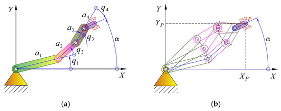
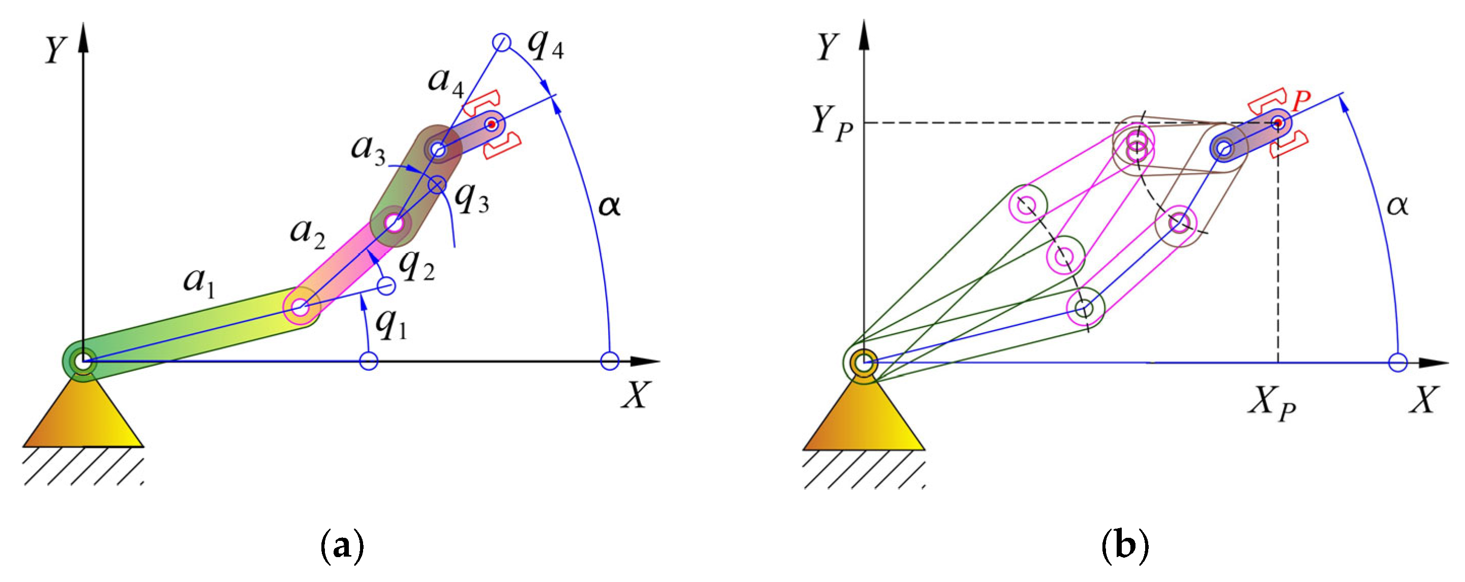
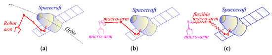
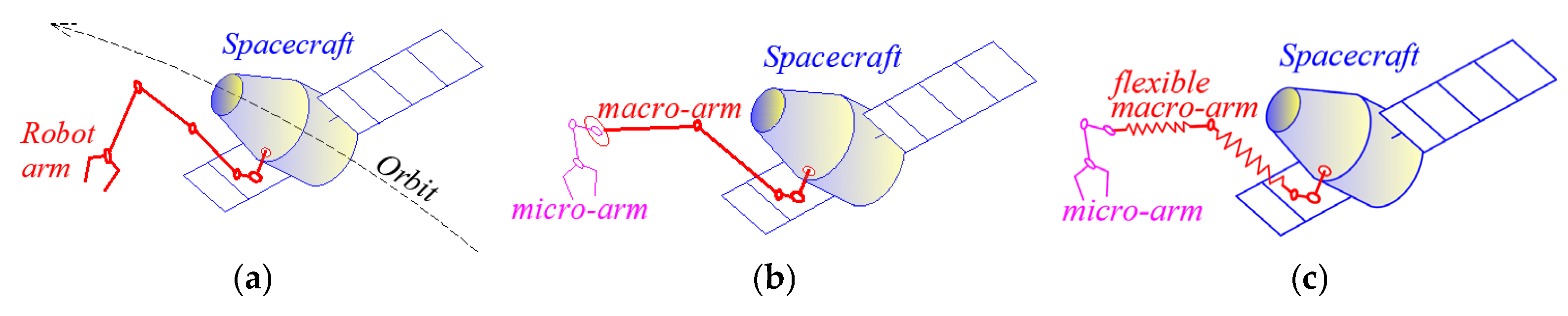
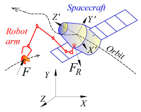
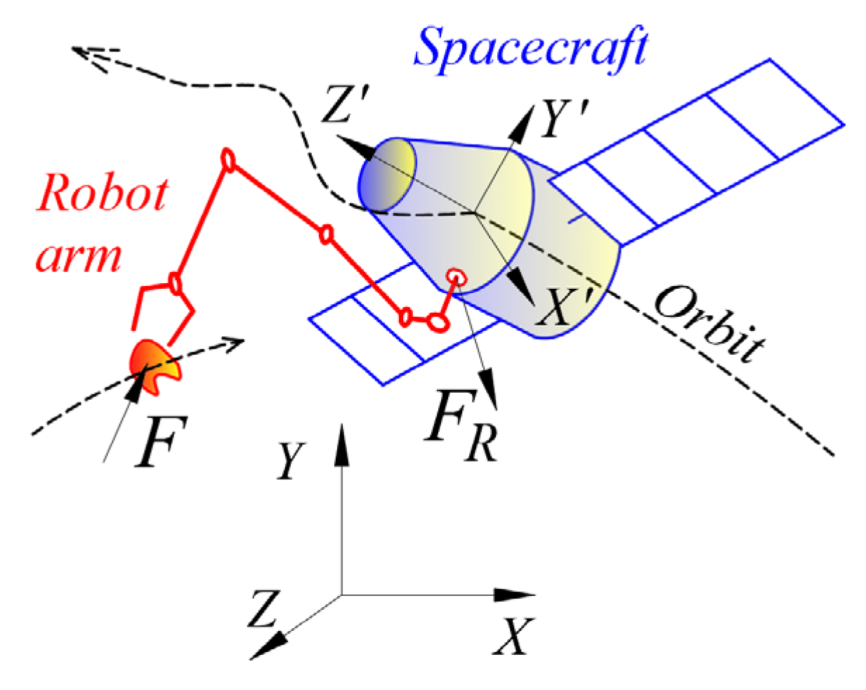
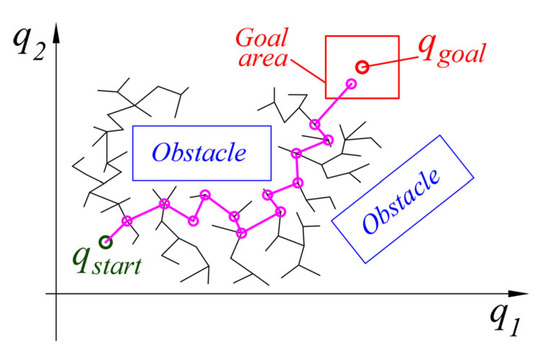
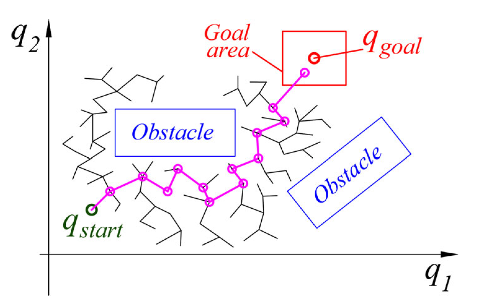
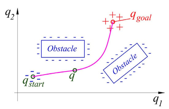
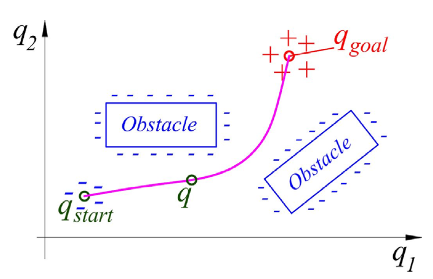
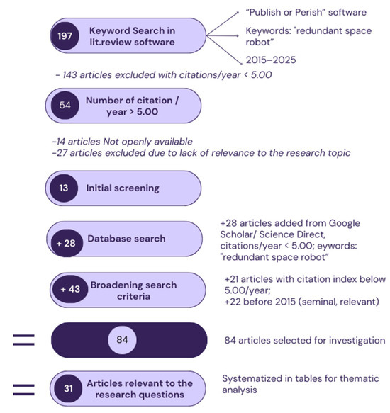
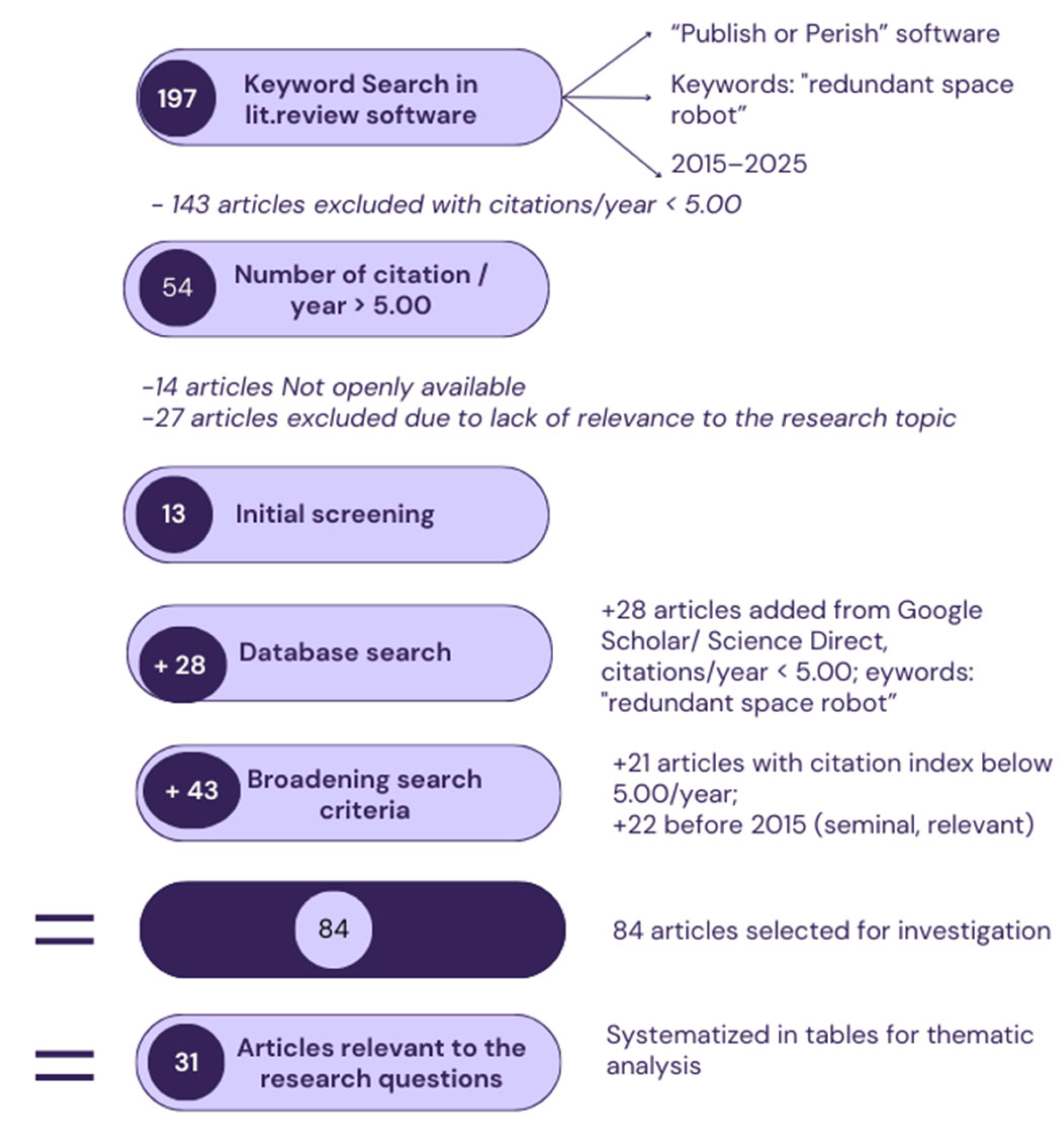
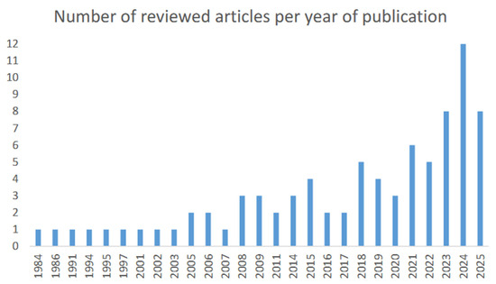
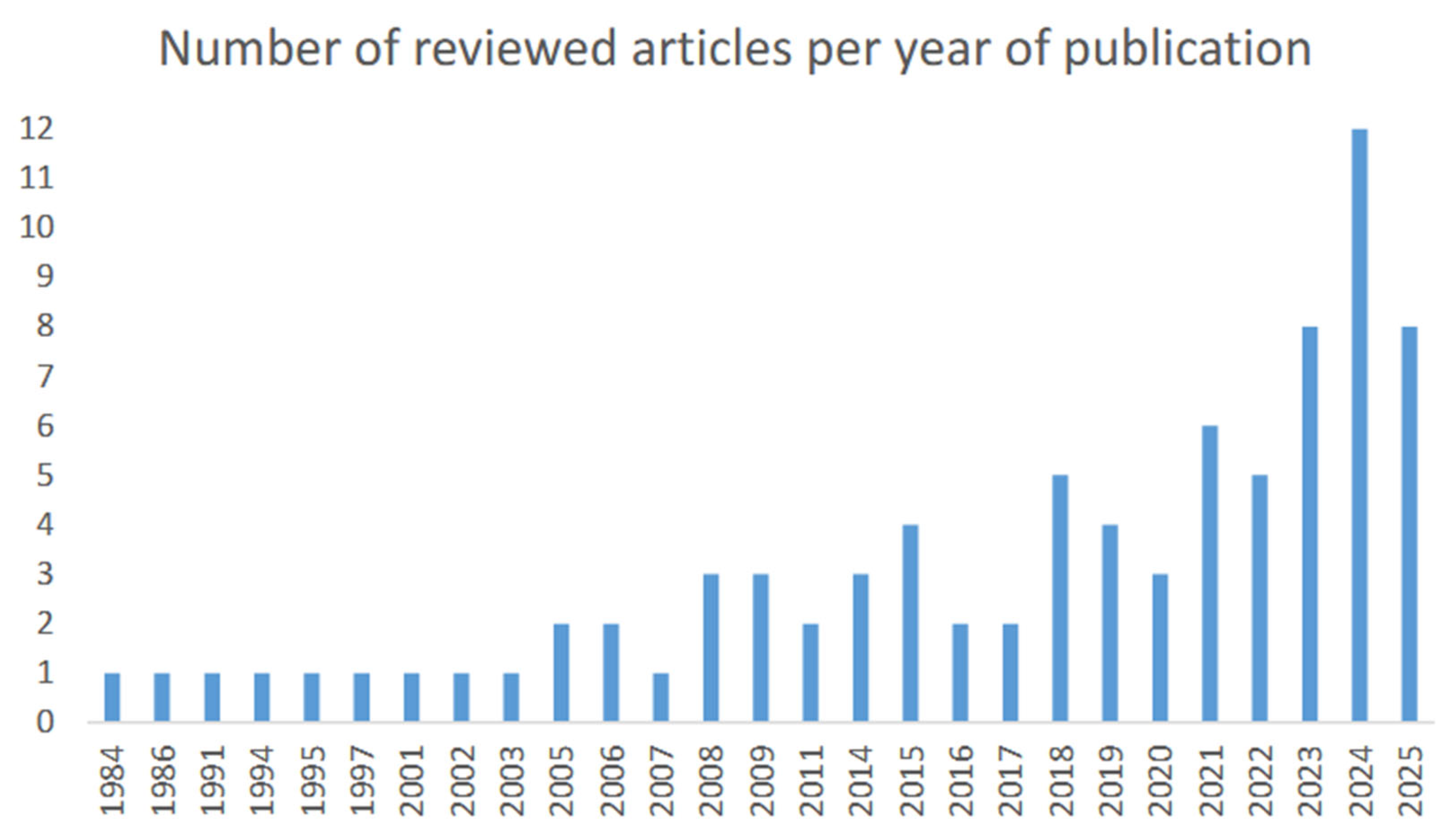
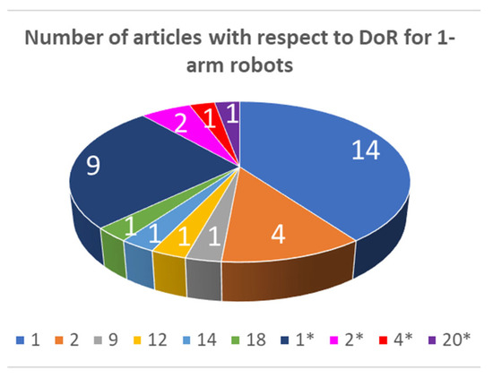
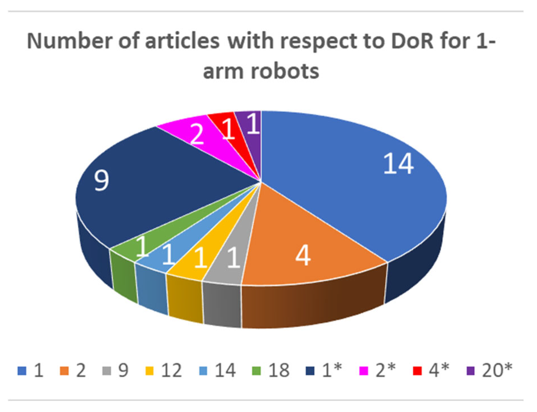
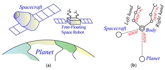
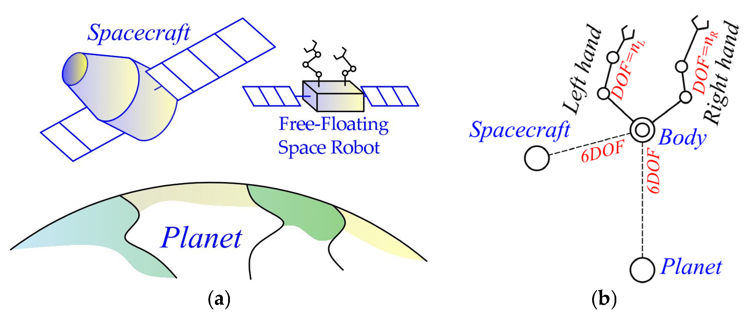
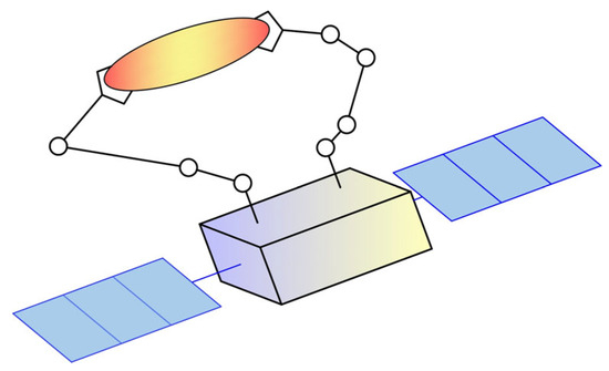
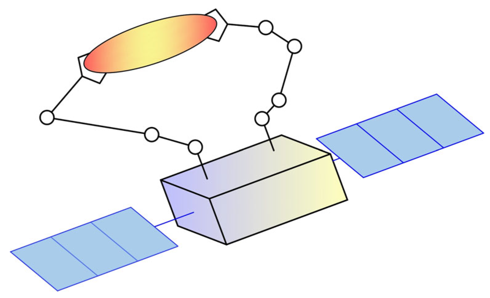
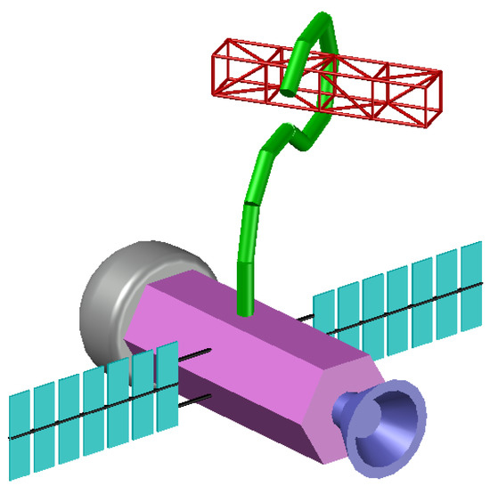
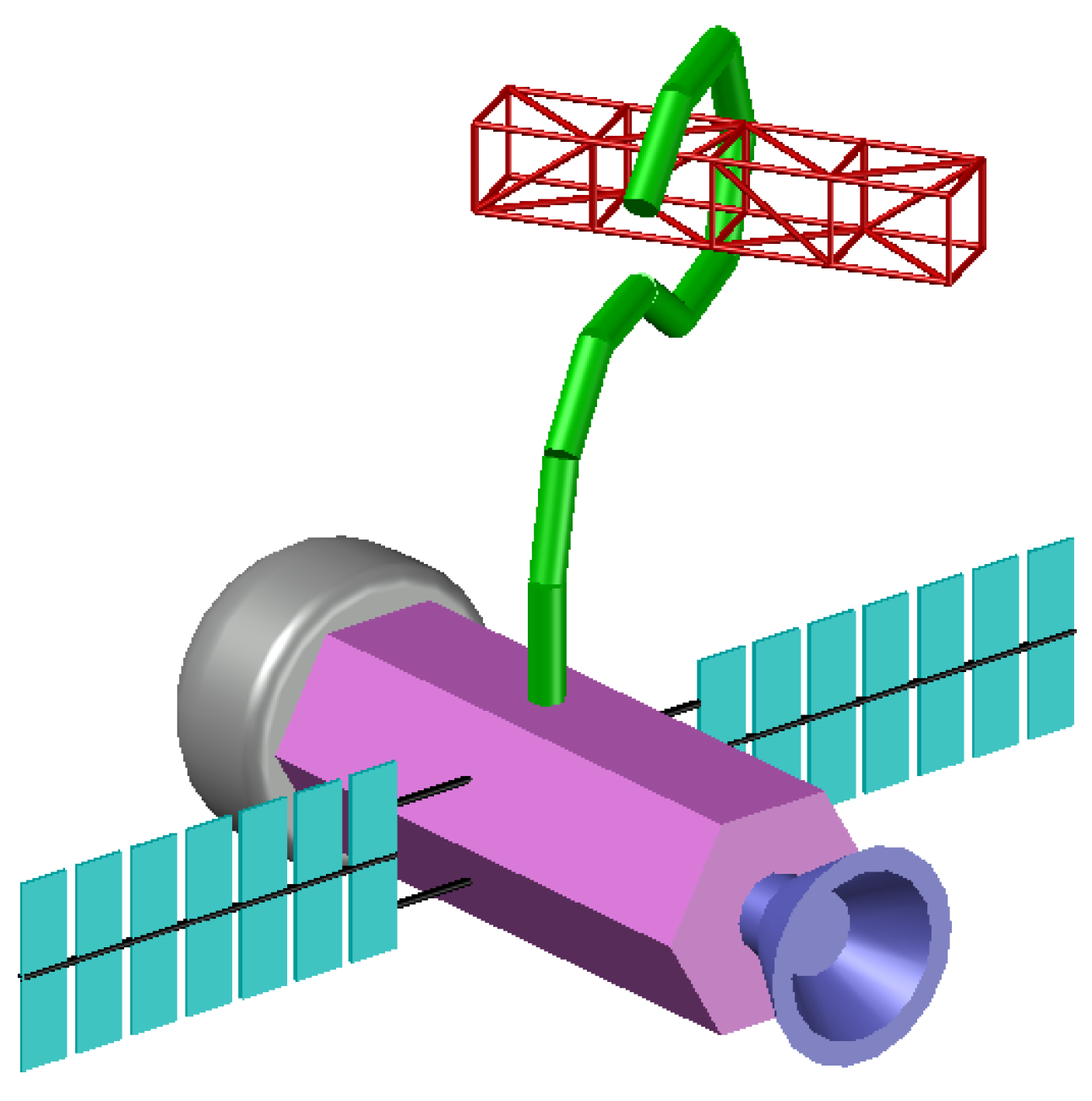
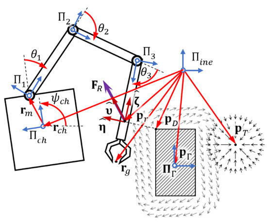
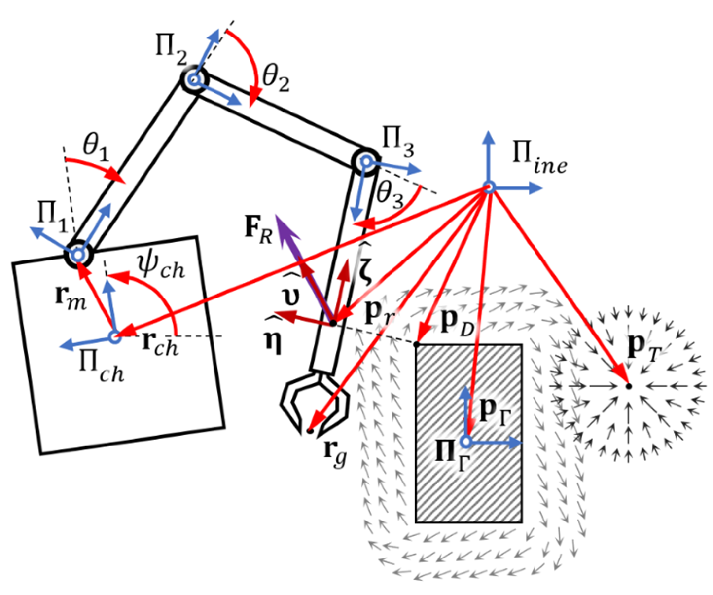
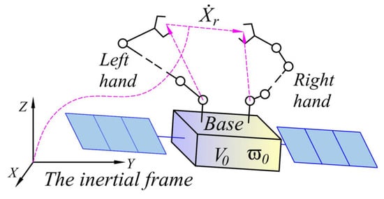
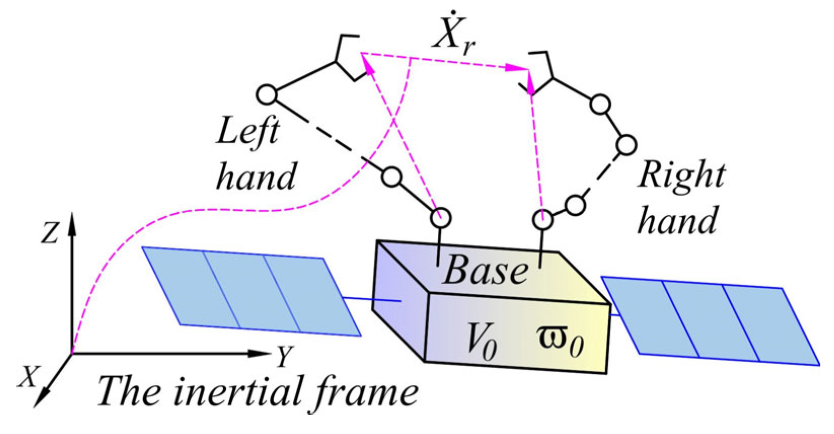

Disclaimer/Publisher’s Note: The statements, opinions and data contained in all publications are solely those of the individual author(s) and contributor(s) and not of MDPI and/or the editor(s). MDPI and/or the editor(s) disclaim responsibility for any injury to people or property resulting from any ideas, methods, instructions or products referred to in the content. |
© 2026 by the authors. Licensee MDPI, Basel, Switzerland. This article is an open access article distributed under the terms and conditions of the Creative Commons Attribution (CC BY) license.