


Abstract
In order to reduce the influence of external radial disturbances on the control accuracy and stability of the vehicle magnetic suspension flywheel battery system during driving, and to further enhance the system’s disturbance rejection ability, this paper designs a control method based on the Accelerated Engineering Fastest Controller (AEFC) and the improved differential optimization algorithm. A mathematical model of the flywheel battery system is established, and the AEFC scheme with engineering disturbance rejection is adopted in the control loop. The improved differential optimization algorithm is used to obtain the optimal control parameters of AEFC, and a multi-criteria optimization function combining tracking error and smoothness is established. The overall control scheme effectively integrates the characteristics of rapid tracking, interference suppression, and rapid parameter adjustment. The experimental results show that compared with the Engineering Fastest Controller (EFC), in the vehicle turning process, the AEFC controller can reduce the offset by 28% during vehicle driving, and compared with the traditional PID control, it can reduce the offset by 41.94%. In the process of vehicle uphill and speed change, the control effect of AEFC also has a significant improvement.
1. Introduction
Different from traditional chemical energy storage technology, the Flywheel Energy Storage System (FESS) uses a high-speed rotating flywheel to store mechanical energy, which has significant advantages of no pollution, strong environmental adaptability, long life and high energy conversion efficiency [1,2,3]. It can be widely used in transportation, aviation, power systems, new energy and other fields, and is one of the most promising energy storage technologies at present, which is highly valued at home and abroad, and its small size advantage is also more conducive to vehicle layout and installation [4]. The FESS’s stable operation is critical; it directly affects the life and application scale of FESSs. The road conditions and driving conditions are typical key problems affecting the robustness of the FESS, and the control accuracy of the magnetic suspension flywheel battery system will directly affect the service quality of the flywheel battery. Therefore, the importance of the control strategy of the magnetic suspension is self-evident [5], so it is necessary to propose a more stable vehicle-mounted flywheel battery system control strategy.
At present, the classic PID control still dominates in industrial process control, and the types of PID applications have become quite diverse [6]. Various studies on PID improvements have also been ongoing without interruption. To overcome the shortcomings of PID and break free from the constraints of the object model, Nonlinear Active Disturbance Rejection Control (ADRC) is proposed and applied to the control of a vehicle magnetic suspension flywheel battery [7]. In [8,9], Model-free control has overcome the limitations of traditional control methods, which are characterized by complex calculations and slow convergence. However, since it is model-free control, the overall robustness and adaptability are limited. And parameter tuning relies on experience and lacks universal guidelines. Moreover, its adaptability to specific conditions is limited. In [10], a method combining quantitative modeling of coupling effects and intelligent parameter adaptive adjustment has been proposed. This method overcomes the theoretical limitation of traditional models that ignore the coupling of degrees of freedom by using interaction factors and solves the engineering challenge of difficult dynamic matching of control parameters under complex working conditions through FA-BPNN. However, it does not take into account the possibility of larger torsional disturbances that may occur during actual vehicle driving. At this time, the applicability and model accuracy of the interaction factors lack verification. In [11], a lateral sway feedback controller based on differential flatness theory has been designed. The controller possesses both high precision and strong robustness. However, the selection of the flat output relies on precise system model parameters. If the actual vehicle parameters (such as the center of mass position and moment of inertia) change, it may lead to the failure of flatness verification and insufficient robustness of the controller. In [12], the author systematically summarized the corresponding modeling methods based on the characteristic differences between suction-type and repulsion-type magnetic bearings and sorted out the corresponding control strategies according to the classification. However, the comparison and optimization of the modeling methods are insufficient, which also makes it difficult to meet the actual needs of the industrial sector. In [13], a method for establishing an analytical model of a magnetic levitation system through a multi-scale approach has been proposed, aiming to build a precise prediction system. However, it overlooked the magnetic flux pinning property of superconducting materials, the dynamic changes of magnetic hysteresis loss, and the stiffness and damping parameters in the model are fixed values. The nonlinear effects of vibration amplitude and frequency on the parameters are not considered. In [14], a method has been proposed that can adapt to unknown fault types without the need for a pre-defined, precise fault model. It only requires a clear understanding of the macroscopic behavior structure corresponding to the fault and can quantify the degree of the fault through parameter estimation, breaking through the limitation of traditional multi-model methods that can only handle known faults. However, it relies on linear and Gaussian assumptions and will fail when dealing with multiple faults. And in [15], an adaptive modeling method based on input-output system identification has been proposed. This method can achieve the dual goals of fault type identification and severity assessment by extracting the energy proportion of the weight matrix coefficients corresponding to the fault characteristic frequencies. However, this method has limitations in terms of model adaptability and scalability, and the balance between algorithm complexity and real-time performance has not been addressed. Furthermore, in the field of model predictive control, a combination of nominal particle characteristics and robust model predictive control (RMPC) is employed. A method for modeling system uncertainties and characterizing observable system dynamic properties using nominal particles (NP) has been proposed [16]. However, due to the three assumptions made when constructing the dynamic model: ignoring pitch and roll motions, assuming that the suspension system and flywheel are rigid bodies and ignoring the aerodynamic effects under high-speed operation. This may lead to a decrease in the matching degree between the model and the actual system, thereby limiting the performance of the control strategy in extreme conditions. Since this method focuses on the robustness of model parameter uncertainty, it is relatively weak in addressing specific radial and torsional disturbances during driving and does not fully meet the control requirements in actual driving scenarios. And in [17], a semi-supervised control strategy integrating the extended state observer (ESO), symmetric barrier Lyapunov function constraints, and a deep belief network (DBN) has been proposed. However, due to the fixed structure of the model lacking adaptability and the strong dependence on training data, the training complexity is high. When deployed in the computationally limited embedded systems of vehicles, it may encounter challenges in real-time performance.
Although the effect of anti-disturbance control is obvious, the structure is more complex, and there is a contradiction between bandwidth and noise, that is, the inadequacy of filtering. In [18], an adaptive resonant filter structure has been proposed, providing a dynamic solution to the amplitude variations caused by high-order harmonics and gate frequency changes. In the pollution control system, the stability of the adaptive method has been thoroughly analyzed, regarding the problem that the conventional PID integration method is not efficient in tracking constant disturbances. In [19], an Engineering Fastest Proportional-Integral Controller (EFPI) and an Engineering Fastest Leading Observer (EFLO) form the Engineering Fastest Controller (EFC) for the project. Its suppression performance for external disturbances on the slope has been improved by 78.6% compared to PI and by 43.7% compared to PID. Subsequently, the Acceleration Engineering Fastest Tracking Filter (AEFTF) and the corresponding parameter Acceleration Engineering Fastest Proportional-Integral (AEFPI) that are further proposed enhanced the external disturbance suppression performance by approximately 9% [20]. In [21], the mechanism of AEFPI has been studied, and the theoretical basis for its substantial improvement in feedback control performance has been provided. And when the control signals of the system are limited, an overshoot phenomenon will occur [22]. Therefore, corresponding measures to anti-windup protection need to be designed.
The structure of EFC is similar to that of the traditional PID controller, but it has good stability, high efficiency, easy parameter setting and better adaptability. However, it has not yet been applied in the control of vehicle magnetic suspension flywheel battery. Parameter tuning is a crucial issue for controllers. The EFC adjusts parameters based on the Ziegler–Nichols model (ZNM), but due to the unstable open-loop nature of the system [23], it is impossible to obtain the corresponding parameters using the ZNM model. Therefore, it is necessary to develop an intelligent and convenient automatic parameter-searching solution [24,25]. In [26], a method for adjusting the PID controller parameters in magnetic bearing control using a particle swarm optimization algorithm and a beluga whale optimization algorithm has been proposed and studied. However, the universality and convergence speed of the aforementioned swarm intelligence algorithms have not been adequately considered.
This paper constructs a synergistic control and optimization framework that deeply integrates the “Acceleration Engineering Fastest Controller (AEFC) architecture with an intelligent multi-objective differential evolution algorithm.” This framework provides a systematic theoretical solution to address the challenges of multi-source disturbance suppression and high-precision, stable control faced by vehicle-mounted magnetic suspension flywheel batteries under complex driving conditions. The research first established a multi-degree-of-freedom dynamic model of the multi-function air-gap magnetic suspension flywheel battery. Building upon this foundation, an enhanced AEFC controller is designed, which integrates the “Acceleration Engineering Fastest Tracking Filter (AEFTF), the Acceleration Engineering Fastest Proportional-Integral controller (AEFPI), and the Engineering Fastest Lead Observer (EFLO).” This design fundamentally strengthens the system’s dynamic response and disturbance prediction capabilities at the structural level. To address the controller parameter tuning difficulties arising from the system’s inherent open-loop instability and strong coupling, this study proposes an improved adaptive differential evolution algorithm incorporating Pareto ranking and crowding distance mechanisms. This control method better meets the actual driving requirements and is more suitable for control in vehicle-mounted flywheel batteries. This algorithm achieves adaptive global collaborative optimization of multiple key AEFC parameters. And corresponding anti-windup protection is designed. Through comprehensive simulation analysis and comparative real-vehicle experiments under multiple operating conditions, the proposed strategy—compared to traditional PID, ADRC, and benchmark EFC methods—demonstrated a maximum reduction in rotor radial displacement of 41.94% during typical disturbance scenarios such as steering and variable-speed hill climbing. This signifies a significant enhancement in the system’s control performance and validates the effectiveness of the proposed framework in improving system disturbance rejection capability and control precision. This research not only pioneers a new pathway for controlling high-performance magnetic suspension flywheel batteries but also provides a referential theoretical framework and a high-performance solution for the intelligent disturbance rejection control of complex electromechanical systems.
2. Mathematical Model of Magnetic Suspension Flywheel Battery
2.1. Magnetic Suspension Flywheel Battery Structure
The model of the multi-function air-gap vehicle magnetic suspension flywheel battery is established in SolidWorks 2023. The key parameters are shown in Figure 1. A set of five degrees of freedom sensors is installed on the top and bottom of the flywheel battery. The axial sensor installed on the top measures the displacement of the flywheel in the vertical direction z, and the radial sensor installed on the side of the virtual inertial spindle, which is used to detect the position of the flywheel in the direction x1 and y1. Torsion sensors are mounted on the bottom side to measure the flywheel position in the x2, y2 directions. It is worth noting that this flywheel battery is a new concept battery due to its high stability, superior energy storage characteristics and being more practical and conducive to large-scale promotion. In addition, it can also be mixed with other powertrains in the vehicle system to protect the original power battery or provide energy recovery to improve energy efficiency.
Figure 1.
Flywheel battery structure and its internal air gap and magnetic circuit.
2.2. Establishment of the Mathematical Model
The vehicle magnetic suspension flywheel battery system has six degrees of freedom, namely the movements along the x, y, and z axes and the rotations around the x, y, and z axes. Among them, the movement along the z-axis is controlled by the axial magnetic bearings and is naturally decoupled from the radial magnetic bearings, being controlled independently. The rotation around the z-axis is controlled by the motor. Therefore, only considering the four degrees of freedom of the movement along the x and y axes and the rotation around the x and y axes, which are controlled by the two radial magnetic bearings, the force is shown in Figure 2. Based on the top view of the structure, a radial xy coordinate system is established. C represents the position of the center, l1 + l2 is the distance between the two radial magnetic bearings on both sides, l1 and l2 are the distances from the magnetic bearings at the 1st and 2nd ends to the center c, x1 and y1 are the displacements of the magnetic bearings at the 1st end along the x and y axes, x2 and y2 are the displacements of the magnetic bearings at the 2nd end along the x and y axes, and xc and yc are the translational displacements of the center c along the x and y axes.
Figure 2.
Diagram of force acting on magnetic bearing.
Based on the force distribution of the magnetic levitation bearing, the kinematic equations of the vehicle magnetic suspension flywheel battery system are established. Based on the Newton–Euler equations for rigid body dynamics, the translational and rotational motions of the flywheel rotor are described by Equation (1). As follows specifically:
where m represents the mass of the flywheel rotor, Fx1 and Fy1 are the electromagnetic forces at the a-end of the x-axis and y-axis, respectively. Fx2 and Fy2 are the electromagnetic forces at the b-end of the x-axis and y-axis, respectively. Jx, Jy, and Jz represent the rotational inertia of the magnetic bearing around the x-axis, y-axis, and z-axis, respectively. Fxr and Fyr are the unbalanced force and external disturbance force, respectively.
When the rotor displacement and control current are both very small, the linear equation set of the electromagnetic force of the magnetic suspension flywheel battery is as shown in Equation (2) below:
where kx and ky represent the force-displacement stiffness, while kxi and kyi represent the force-current stiffness.
Let the state variables X, control variables U and output variables Y of the system be as follows:
Then, the state equation of the four-degree-of-freedom active magnetic bearing system is:
where A is the state matrix, and B is the control matrix.
The specific parameters in the formula are as follows:
3. Design of Magnetic Suspension Flywheel Battery Anti-Disturbance Controller
The AEFC control scheme for the magnetic suspension flywheel battery system is shown in Figure 3.
Figure 3.
Anti-disturbance control strategy for vehicle magnetic suspension flywheel battery system under the control of AEFC with improved ADE.
3.1. Accelerated Engineering Fastest Controller
3.1.1. Accelerated Engineering Fastest Tracking Filter
To construct an Accelerated Engineering Fastest Tracking Filter (AEFTF), one must understand its key structure. Accelerated means that its structural design is aimed at achieving a faster dynamic response speed and interference suppression capability than the traditional fastest controller (EFC), and it does not directly use the second derivative (acceleration) of the system as the feedback signal. The mathematical expressions of the Fastest Tracking Filter (FTF) and the accelerated optimal tracking filter are as follows:
where Tw represents the window time length of FTF, TT is the tracking time constant of AFTF.
The unit step output of AFTF is:
where PAFTF(t) represents the process output of AFTF under a step input, and aPV represents the acceleration of the output of AFTF.
In practical engineering applications, when the process being filtered reaches a steady state, there will be a certain steady-state error between the output and the input of the AFTF. To solve this problem, it is necessary to carry out engineering improvements on the AFTF. The specific method is to approximate the output response of the AFTF under the action of a unit step input signal as the superposition of 1st to nth pure lag links, thereby obtaining an approximate AFTF model (AAFTP). As shown in the following:
where fAAFTF(s) is the transfer function of AAFTF. n represents the number of pure lag sections in series. The larger the value of n, the higher the approximation degree between AAFTF and AFTF.
In engineering, the pure lag component is typically approximated by a first-order inertia filter (FOIF). Thus, by replacing the pure lag component in the Approximated Acceleration Fastest Tracking Filter (AAFTF) with FOIF, the Acceleration Engineering Fastest Tracking Filter (AEFTF) can be derived. As shown in the following:
where TFOIF is the time constant of FOIF.
Through extensive computational simulations, it is found that when n = 14 and TT = 8 s, the AEFTF obtained the process output PAEFTF(s) in response to a unit step input, and its output characteristics are compared with those of FOIF and AFTF. The results are shown in Figure 4. According to the results, it should be noted that although AFTF exhibits a slightly slower initial response compared to FOIF, it achieves a faster overall tracking speed and better steady-state performance. Moreover, when the input acceleration is zero, AFTF can maintain a constant output acceleration. The AEFTF obtained through engineering approximation has a high fitting accuracy for this characteristic. The 14th-order filter is widely used in theoretical modeling and simulation, typically for achieving a high-precision approximation of the ideal filter characteristics. However, in actual real-time control systems, we usually employ techniques such as reduced-order approximation, model reduction, or structural optimization to achieve practical applications in engineering. Reducing the filter order to a more practically valuable one (such as 3rd or 4th order) will significantly increase the calculation speed, but it may result in larger overshoot, longer adjustment time, and increased low-frequency phase lag, which may affect the dynamic response of the system.
Figure 4.
Diagram of filter process output characteristics.
3.1.2. Accelerated Engineering Fastest Proportional-Integral Controller
AEFTF serves as the theoretical foundation and structural framework for constructing accelerated engineering fastest integrators. Under this system, when designing a conventional integrator (CI), the FOIF is typically placed in the positive feedback loop of the system. The specific structural block diagram is shown in Figure 5.
Figure 5.
Block diagram of the transfer function.
By leveraging its phase lead and gain regulation characteristics, the dynamic response speed and steady-state accuracy of the system are enhanced, thereby achieving effective acceleration of the signal integration process and noise suppression while maintaining a simple structure. This construction method not only optimizes the dynamic performance of the integrator but also provides a clear parameterized design path for engineering implementation. As shown in the following:
Similarly, the engineering fastest integrator AEFI can be constructed using AEFTF. Its specific expression is:
where fAEFI(s) represents the transfer function of AEFI, and TAEFI is the integration time constant. When n = 14 and s approaches ∞ or 0, fAEFI(s) can be simplified to the following:
Let TAEFI = T1. By comparing the engineering fastest integrator with the conventional integrator, it can be observed that when s approaches ∞, in the transfer function, the higher-order terms dominate, and the lower-order terms can be disregarded. The gain of AEFI is 0.1192 times that of CI; this indicates that AEFI exhibits a lower gain characteristic at extremely high frequencies. This also helps to enhance the stability of the system. When s is equal to 0, the constant term dominates in the transfer function. The gain of AEFI is 1.4202 times that of CI. This means that the AEFI has a higher gain at low frequencies (in a steady state) and responds more strongly to slowly varying signals. Therefore, by using AEFI to construct AEFPI, its transfer function can be expressed as the following:
where KAEFPI is the proportional gain parameter of the accelerated engineering’s fastest proportional-integral controller (AEFPI).
3.1.3. Engineering Fastest Leading Observer
To effectively enhance the dynamic response quality and disturbance rejection performance of the system, especially when operating in a wide speed range to cope with strong gyroscopic effects and coupling interference, the control loop requires an observation mechanism that can accurately and in advance obtain the trend of system state changes. Although traditional lead compensation devices can provide phase lead, they are sensitive to noise, and it is difficult to achieve a good balance between the lead amount and disturbance rejection capability. Therefore, based on the core concept of FTF, this section constructs an Engineering Fastest Leading Observer (EFLO) with high phase lead efficiency and strong disturbance rejection capability.
This observer not only has a simple structure and clear physical meanings of parameters, but also can provide the controller with advanced predictive information of the system response. It is acknowledged that the derivative term in a conventional PID controller also provides a form of predictive action by extrapolating the error trend. However, the EFLO proposed here differs in several key aspects: (1) It is constructed based on the FTF framework, which allows for a more tailored phase lead profile across a specific frequency band. (2) The structure incorporates explicit filtering stages (FOF and FTF in the feedback path), making it inherently more robust to high-frequency measurement noise compared to a pure derivative term, which often requires additional external filtering. (3) The EFLO can be viewed as an observer that synthesizes a predictive signal from the filtered error, potentially offering a superior trade-off between prediction accuracy and noise immunity for the specific dynamics of the magnetic suspension system. Its transfer function fEFLO(s) is defined as follows:
where fEFLO(s) and TEFLO are the transfer function and the equivalent lead-time constant of EFLO, respectively, and KC is the transformation gain. fFOF(s) and TFOF represent the transfer function and the filter time constant of the first-order filter.
TEFLO determines the intensity and duration of the lead effect. KC is a key design parameter, requiring KC ≫ 1. The purpose is to significantly amplify the signal processed by the first-order filter FOF in the forward channel and compare and synthesize it with the output of FTF in the feedback loop, thereby constructing a strong phase lead effect within a specific frequency band. FOF here mainly serves to smooth the input signal and suppress high-frequency noise, ensuring the quality of the internal signals of the observer and avoiding the failure of the observer due to noise amplification. fFTF(s) introduces specific phase lag and amplitude attenuation characteristics in the feedback loop. Working together with the pre-existing FOF and the high-gain KC, it ultimately shapes the required leading phase peak in the open-loop transfer function.
The core mechanism of EFLO lies in utilizing the feedback characteristics of large gain KC and FTF to modify the zero-pole distribution of the system. In the frequency domain, its amplitude-frequency characteristic shows an appropriate gain near the cutoff frequency, while the phase-frequency characteristic can generate a significant phase lead peak within the target frequency band.
As shown in Figure 6, when the parameters are set as TEFLO = 253 s, TFOF = 5.58 s, the phase characteristics of EFLO reach a peak of 88.73° at a specific frequency. This high phase margin of approximately 90° indicates that EFLO can significantly improve the system’s stability and responsiveness, allowing it to better handle dynamic changes and disturbances.
Figure 6.
Diagram of frequency characteristics of EFLO. (a) Amplitude margin. (b) Phase margin.
3.1.4. Anti-Windup Implementation for AEFPI
In practical applications, actuator saturation may lead to integral windup, especially under large disturbances or high-dynamic operating conditions. To enhance the disturbance rejection capability of the proposed AEFC, an implicit anti-windup structure based on the conditioning technique is incorporated into the AEFPI design. The modified control law is expressed as:
where uc(s) is the unlimited control signal, ulim(s) is the saturated actuator output after physical limits, and TAEFPI is the integral time constant of the AEFPI. This structure ensures that when the actuator saturates, the integral state uf(s) is dynamically conditioned to prevent accumulation of excessive integration error, thereby avoiding overshoot and instability during saturation recovery.
This anti-windup mechanism is implemented in the discrete-time controller without adding significant computational overhead, and it maintains the original dynamic performance of AEFPI under normal operating conditions. The stability of the closed-loop system with anti-windup is preserved, as the conditioning scheme does not alter the nominal controller dynamics when not in saturation.
3.2. The Parameter Optimization Problem of AFEC
The optimization of the controller parameters is a crucial step in achieving its ideal control performance. For the Accelerated Engineering Fastest Controller (AEFC), parameter tuning directly affects the system’s performance in terms of dynamic response, disturbance resistance, and stability. In traditional engineering, the Engineering Fastest Controller (EFC) often adjusts parameters based on the Ziegler–Nichols (Z-N) tuning rule. This method relies on the critical gain and period of the system and is suitable for stable objects with self-balancing capabilities. However, the magnetic suspension flywheel battery system itself is an open-loop unstable system and does not possess self-balancing characteristics, so the Z-N and other empirical tuning methods based on models cannot be directly applied. Moreover, when operating over a wide speed range, the magnetic suspension flywheel battery system faces significant dynamic coupling effects among its degrees of freedom, particularly the pronounced gyroscopic coupling, along with external disturbances, which further increase the complexity of parameter tuning.
To address the aforementioned issues, this paper employs an optimization algorithm based on swarm intelligence to automatically optimize the parameters of the AEFC controller. The control performance of AEFC is mainly determined by three key parameters: proportional gain KAEFPI, lead observation time constant TEFLO, and integral time constant TAEFPI. These parameters collectively affect the tracking accuracy, response speed, and disturbance rejection capability to disturbances of the system. If the parameters are set improperly, it may result in excessive overshoot, prolonged adjustment time, or instability under disturbances. To comprehensively evaluate the performance of the controller and meet the disturbance resistance requirements under different rotational speed conditions, this paper constructs a multi-objective optimization function, which takes into account both the tracking error and the smoothness of the control signal. The objective function is defined as follows:
where Pik represents the parameter matrix of AEFC, which includes KAEFPI, TEFLO and TAEFPI for each degree of freedom. es(t) is the tracking error of the s-th degree of freedom, and u(t) is the control input signal, whose smoothness is reflected by the rate of change. w1 and w2 are the weight factors for tracking error and smoothness, respectively, used to balance the system’s dynamic response and control energy consumption. Tmax is the upper limit of the simulation time.
The design of this objective function takes into account the comprehensive consideration of the dynamic quality of the system and the burden on the actuator: the tracking error term ensures that the system output can quickly and accurately follow the reference signal, the smoothness term is used to suppress the drastic fluctuations of the control signal, reduce the impact on the actuator, and improve the reliability and lifespan of the system in actual operation.
3.3. Differential Evolution Algorithm
The differential evolution algorithm is an optimization algorithm based on the evolution of individual members of a population. It has the characteristics of a simple principle, requiring fewer parameter adjustments, and strong global exploration ability. The operation steps of the differential evolution algorithm include mutation, crossover, and selection. Its core idea is to use the differential information between different individuals in the population to perform mutation operations and then control the crossover operation of population individuals through a random probability mechanism. If the randomly generated value is greater than the crossover probability factor, the parent individual is selected; if it is less than the crossover probability factor, the newly generated contribution vector is selected. Finally, the final offspring population is selected based on the size of the fitness function value. During the iterative process of the differential evolution algorithm, three parent individuals need to be randomly selected to generate differential information in the mutation strategy and serve as the base vector, the individual Mutanti,t generated through the mutation strategy is called a “contribution vector”, the individual Childi,t generated by the crossover strategy through the combination of the parent individual and the contribution vector is called a “test vector”. Finally, a new population is generated by the greedy selection strategy together with the parent individual and the test vector, and the process repeats until the algorithm sets the size of the fitness function value or the maximum number of iterations is completed. The control parameters of the differential evolution algorithm mainly include: the population size Np, the mutation factor F in the mutation strategy, and the crossover probability factor CR in the crossover strategy.
- (1)
- Population Initialization
In the differential evolution algorithm, there are multiple individuals within the population, and each individual represents a solution to the optimization problem. The parameters of the current algorithm are set as follows: the population size is Np, the individual dimension is D, the mutation factor is F, and the crossover probability factor is CR. Then, the current population pt can be described in the following:
where t represents the current generation number and t = 0, 1, 2, …, Tmax. xi,t represents the vector of the i-th individual in the t-th generation of the population. x1i,t represents the value of the 1st dimension of the i-th individual in the t-th generation of the population.
- (2)
- Mutation Operation
The term “mutation” originates from the genetic mutation phenomenon in biology. In evolutionary algorithms, mutation refers to the behavior where a parent individual changes a certain value through a certain mutation strategy. The advantage of this behavior is that it can increase the diversity of the population, escape from local optima, and help explore the global optimal solution. In the differential evolution algorithm, the parent individuals are mutated based on the differential information among the individuals in the population. The mutation operation involves selecting multiple parent individuals (Parenti,t) from the current population and generating a mutation vector (Mutanti,t) through the mutation strategy. The different mutation strategies are represented in the form of “DE/x/y”, where x indicates the way of selecting Parenti,t in the mutation strategy, and it is usually randomly selected as “rand” or the optimal individual Parentbeat,t from the current population. y represents the number of differential vectors in the mutation strategy. Common mutation strategies are as follows:
DE/rand/1:
where i1, i2, i3 ∈ [1, NP] represents three randomly generated integers, and i1 ≠ i2 ≠ i3 ≠ i. F ∈ (0, 1] is a variant factor; it is used to control the size of the differential vector (Parenti2,t − Parenti3,t) and determine the variation step size.
DE/rand/2:
This strategy uses randomly selected Parenti1,t as the base vector, and by randomly selecting another 4 parent individuals to form two differential vectors (Parenti2,t − Parenti3,t) and (Parenti4,t − Parenti5,t), it determines the direction of the search. Compared with Equation (18), this strategy enables the algorithm to search for the optimal solution over a wider range, enhancing the global capability of the algorithm. However, this strategy has a long computing time and a slow convergence speed.
DE/best/1:
where Parentbeat,t is the best individual in the contemporary population.
This strategy uses Parentbeat,t as the base vector, and determines the search direction through a difference vector (Parenti1,t − Parenti2,t). Compared with Equation (18), it has stronger local search capabilities and a faster convergence speed, but it is prone to causing the algorithm to become stuck in a local optimum.
DE/best/2:
Compared with Equation (21), a new difference vector (Parenti3,t − Parenti4,t) is added to determine the search direction. This strategy can retain strong local search ability and reduce the convergence speed of the algorithm, but it still has the problem of premature convergence.
DE/current to rand/1:
This strategy uses the current parent individual Parenti,t as the base vector, and randomly selects three parent individuals that are different from the current individual. Through two difference vectors (Parenti1,t − Parenti,t) and (Parenti2,t − Parenti3,t), the direction of the search is determined. Some information of the current individual is retained to maintain the local search ability of the algorithm, but the convergence speed of the algorithm is relatively slow, and the parameter settings are relatively sensitive.
DE/current to best/1:
This strategy uses Parenti,t as the base vector. By integrating the optimal individual of the population into the differential vector, two differential vectors (Parentbest,t − Parenti,t) and (Parenti2,t − Parenti3,t) are formed to determine the direction of the search. This strategy can achieve a good balance between exploration and exploitation, but it sacrifices the stability of the algorithm and fails to escape from the local optimal solution.
For the contribution vectors obtained through mutation operations, the variables in some dimensions may exceed the defined range of the independent variables. In such cases, boundary handling should be performed. For values exceeding the upper limit, they should be assigned the upper limit value; for values exceeding the lower limit, they should be assigned the lower limit value.
- (3)
- Interlace Operation
After the mutation operation is completed, the mutation vector Mutanti,t and the parent individual Parenti,t will undergo crossover operations according to the crossover strategy, generating the trial vector Childi,t. The common crossover methods are as follows:
Binomial cross:
The binomial crossover operation, as the most widely used crossover method at present, has achieved relatively satisfactory results. The crossover strategy is as follows:
where u represents the dimension, with u = 1, 2, …, D. urand denotes a randomly selected integer within the range [1, D].
Exponential crossover:
For the information of the parent individuals in each dimension, randomly select the starting point for crossover, and continuously perform the crossover operation. The termination condition is to meet the specified conditions of the crossover probability factor CR.
- (4)
- Selecting Operation
After completing the previous crossover operation, a trial vector Childi,t is generated to minimize the problem: compare the fitness levels of the parent individual Parenti,t and the trial vector Childi,t, and select the individual with the smaller fitness value to enter the next iteration calculation. The selection strategy is as follows:
where Parenti,t+1 represents the new generation population, t is the current evolutionary generation number, f(Childi,t) is the fitness value of the test vector, and f(Parenti,t) is the fitness value of the parent individual.
The individual members of the population selected through this strategy can effectively ensure that the population becomes better and better or remains unchanged and will not cause the population to deteriorate. As shown in Algorithm 1, it is the pseudo-code table of the differential evolution algorithm.
| Algorithm 1. Pseudo-code of differential evolution algorithm |
| Input: Population size NP, mutation factor F, crossover probability factor CR, maximum evolutionary generation Tmax. |
| 1: Random initialization of population. |
| 2: Calculate the fitness values of individuals in the population. |
| 3: t = 1 |
| 4: while t Tmax |
| 5: for i = 1 to NP |
| 6: Randomly select i1, i2, and i3, and ensure that i1 i2 i3 i. |
| 7: Generate contribution vector. |
| 8: Cross-boundary handling. |
| 9: Generate the test vector. |
| 10: Calculate the fitness of the test vector. |
| 11: end for |
| 12: for i = 1 to NP |
| 13: if f(Childi,t) ≤ f(Parenti,t) |
| 14: The test vector becomes the new generation of individuals. |
| 15: else |
| 16: The parent individuals become the new generation of individuals. |
| 17: end if |
| 18: end for |
| 19: t = t + 1 |
| 20: end |
| Output: the optimal individual |
3.4. Introduction of Parameter Adaptive Improvement Strategy
The DE algorithm possesses characteristics such as high reliability and strong disturbance rejection capability. Since the parameter tuning of the DE algorithm requires relatively little effort, choosing a simple parameter tuning strategy can achieve satisfactory results. As an evolutionary algorithm, the DE algorithm may also encounter phenomena such as search stagnation and premature convergence. To address the search stagnation and premature convergence that may occur in the DE algorithm, the important control parameters, the mutation factor F and the crossover probability factor CR, are adaptively adjusted to reduce the interference from human factors. Through the iterative process, the mutation factor F and the crossover probability factor CR are dynamically changed to guide the algorithm’s search towards the optimal solution. A reasonable balance is achieved between the convergence speed and the ability to search for the optimal solution. The adaptive differential evolution algorithm (ADE) is an improved evolutionary algorithm developed based on the traditional differential evolution algorithm.
The mutation factor F and crossover probability factor CR of the ADE algorithm are two key parameters that jointly determine the performance of the algorithm. The mutation factor F controls the amplitude of the differential vector and directly affects the convergence speed and global exploration ability of the algorithm: when the F value is small, the algorithm has strong local search ability and runs quickly, but it is prone to premature convergence; when the F value is large, the global exploration ability is enhanced, but the convergence speed will slow down. The crossover probability factor CR mainly affects the diversity of the population: when the CR is small, the offspring information mostly comes from the parent, the evolution is stable, but the diversity is insufficient; when the CR is large, the offspring is more from the mutated individuals, which helps to increase the probability of finding the optimal solution. Both of these parameters need to be dynamically adjusted according to the evolution stage: in the early stage of the algorithm, to increase diversity and avoid premature convergence, the CR should take a larger value; in the later stage of the algorithm, to conduct local fine search, the CR needs to be reduced to retain more current individual information. In terms of specific implementation, mutation adopts the strategy of Equation (18), selecting three parent individuals, and the mutation factor F follows a normal distribution with the dynamically calculated Fk as the expectation and 0.1 as the standard deviation; crossover adopts the strategy of Equation (23), and the crossover probability factor CR also follows a normal distribution with the dynamically calculated CRk as the expectation and 0.1 as the standard deviation. Please refer to Equations (27) and (28) for details:
where Fmax represents the maximum value of the variation factor, Fmin represents the minimum value of the variation factor, CRmax represents the maximum value of the crossover probability factor, and CRmin represents the minimum value of the crossover probability factor, g represents the current generation number, gmax represents the maximum generation number.
3.5. Introduction of Multi-Objective Selection Strategy
The DE algorithm has strong global optimization capabilities and high reliability. Through the proposed parameter adaptive strategy, it can more effectively reduce the involvement of human factors, improve objectivity and the performance of the algorithm. However, its selection operation is still a traditional selection strategy. For the traditional DE algorithm, its selection operation is based on comparing the fitness levels of each individual. In the traditional selection strategy, some individuals with high fitness may occupy too many selection opportunities, resulting in the loss of population diversity and causing the algorithm to converge prematurely and fall into a local optimal region. At the same time, the traditional strategy may be overly concentrated on certain objectives, leading to an uneven distribution of the Pareto front. To address these issues, this study improves the ADE algorithm by introducing non-dominated sorting and crowding distance sorting, replacing the traditional selection strategy. By using the non-dominated ranking information and crowding distance information of individuals, a new offspring population is generated. This approach can better balance the convergence of the algorithm and the uniformity of the Pareto optimal solution distribution.
Non-dominated sorting:
Let the set of all individuals in a population be denoted as Q, and the population size be Np. The number of optimization objectives is t. Qi represents an individual in the population. The following steps are executed:
Initialize the set HQi = KQi = 0.
If Qi is non-dominated with respect to Qj (i ≠ j), then add Qj to HQi: HQi = HQi ⋃ Qj.
If Qj is non-dominated with respect to Qi (i ≠ j), then increase the number of dominant solutions for Qi: KQi = KQi + 1.
If KQi = 0, it indicates that no individual is superior to Qi. Then, Qi is classified as the first non-dominated frontier, and ranki is set to 1. Qi is placed in the set of the first non-dominated frontier.
Set i = i + 1, then continue to execute the previous step until all individuals have been classified.
Crowding degree distance:
In this study, the method of calculating the crowding degree is employed to ensure the distribution and diversity of the population. Firstly, the crowding distance of individuals is calculated. The crowding distance is used to represent the density of solutions around each individual. Individuals with larger crowding distances are given priority, avoiding excessive concentration of individuals and protecting the diversity of the population.
In the problem of dual-objective optimization, the expression of the crowding distance for individual i is:
where f1 represents the first objective function, while f2 represents the second objective function. f1(i) denotes the value of individual i on the first objective function, and f2(i) represents the value of individual i on the second objective function.
As shown in Figure 7, the congestion distance of individual i is the sum of the length and width of the rectangle formed by the dotted line. The dashed boxes in the figure usually represent the local search area of the current solution i.
Figure 7.
Diagram of individual crowding distance.
When the target is multi-objective, the congestion distance of individual i is:
where r represents the number of objective functions.
For the differential algorithm with parameter adaptation, non-dominated solution set sorting and crowding distance sorting are introduced. Before generating the new offspring population, the selection strategy is improved. The parent vectors and the trial vectors after crossover are added to the temporary population. The dominance relationship between the parent vectors and the trial vectors after crossover is compared. This operation resulted in the size of the temporary population ranging from Np to 2Np. The non-dominated solution set sorting is performed on the temporary population to obtain the non-dominated frontier. The individuals in the same frontier are sorted by crowding distance, and the first Np individuals are selected to become the offspring individuals. The truncated process is shown in Figure 8. The arrows in the figure usually represent the dominance relationship between individuals. The arrows point from the dominant individual to the subordinate individual, meaning that the direction of the arrow indicates that the former dominates the latter. The dashed lines in the figure generally represent the boundaries between different non-dominated layers.
Figure 8.
Truncated flowchart.
For all multi-objective optimization algorithms, it is necessary to balance global search and local search. The adaptive differential evolution algorithm has strong global search capabilities, is highly adaptable and requires fewer parameter adjustments. These are its advantages. However, its local search ability is somewhat weaker. Introducing non-dominated sorting and crowding distance sorting can enhance the local search ability while ensuring population diversity. Non-dominated sorting pays more attention to the solutions at the Pareto frontier, guiding the algorithm to focus more on the potential optimal solution regions, thereby enhancing the local search ability. Crowding distance sorting avoids the concentration of solutions at the Pareto frontier, effectively maintaining population diversity. The improved algorithm flow is shown in Figure 9.
Figure 9.
Flowchart of the improved ADE algorithm.
3.6. Introduction of Random Sorting Mutation Strategy
The mutation strategy is of vital importance in the ADE algorithm. By exploring unknown areas and expanding the search scope, it enables the algorithm to escape from the local optimal region and enhance the global search. For the ADE algorithm, the selected mutation strategy is shown in Equation (18), and the mutation strategy is achieved by calculating the differential vector to explore the unknown areas. This algorithm requires selecting three parent individuals, Parenti1,t, Parenti2,t, and Parenti3,t, during the mutation process. If strategies such as DE/rand/1 and DE/rand/2 are adopted, the selection of these three parent individuals is random. This operation helps enhance the global exploration ability and makes the algorithm less likely to become stuck in local optima. However, when the algorithm enters the later evolutionary stage and conducts searches within a relatively small local space, its search ability is weak, and the convergence speed is slow. If the mutation strategies such as DE/best/1, DE/best/2, DE/current to rand/1, and DE/current to best/1 are selected, the selection of the three parent individuals should utilize the optimal individual in the current population. This operation can effectively enhance the algorithm’s search ability in the local space, and the convergence speed of the algorithm is faster. However, it is not conducive to the algorithm’s exploration behavior in the global scope at the initial stage, and it is prone to obtaining a local optimal solution.
Therefore, in order to enable the differential evolution algorithm with adaptive parameter strategy to have the ability to better regulate the relationship between global exploration behavior and local exploration behavior, this study adopts an adaptive differential mutation strategy based on random sorting to select three parent individuals, namely ParentPareto1, ParentPareto2, and ParentPareto3,t. The mutation strategy of the original algorithm is improved to enable the algorithm to better adapt to different optimization problems. The random sorting differential mutation strategy is used during the evolution process, where individuals are sorted based on the number of dominations among them. Individuals with fewer dominations are placed earlier, and the ones with fewer dominations are more excellent. The first n individuals are selected to form an elite group, and then three individuals, namely ParentPareto1, ParentPareto2, and ParentPareto3,t are randomly selected from these n individuals. ParentPareto1, ParentPareto2, and ParentPareto3,t contain the information of the excellent individuals in the current population and can promote the evolution of the population. Compared with the traditional mutation strategy in Equation (18), this study proposes the mutation strategy “DE/Pareto to rand/1”, which is expressed as Equation (31) below:
where ParentPareto1, ParentPareto2, and ParentPareto3,t is three randomly selected individuals from the first n/Np individuals that dominate in the population. The calculation formula is as shown in Equation (32):
where Xi represents the parent individual, i1 ≠ i2 ≠ i3 ≠ i.
To present the variation strategy of the improved algorithm more intuitively, the flowchart of the improved algorithm is shown in Figure 10.
Figure 10.
Flowchart of the improved ADE algorithm with random sorting.
Regarding the random sorting operation, after ranking all individuals in a non-inferior manner, the first n/Np individuals of the population are selected. Among these individuals, a random selection operation is carried out. For the non-inferior ranking of individuals, the Pareto solutions of the current population that are excellent are found. The core of this is to draw on the idea of DE/best/1, where the differential vector uses the global optimal solution, and at the same time enhances the local exploration ability and convergence speed of the algorithm. Among the first n/Np individuals, a random selection is conducted. The core of this is to draw on the idea of DE/rand/1, where individuals are randomly selected, simultaneously enhancing the algorithm’s ability to explore unknown areas and expand the search range, thereby improving the adaptability of the adaptive differential evolution algorithm to different problems. The specific pseudo-code is shown in Algorithm 2 below:
| Algorithm 2. Pseudo-code of an improved adaptive differential evolution algorithm for stochastic sorting |
| Input: Population size Np, parameter dimension, number of objective functions, maximum and minimum values of mutation factor F, Fmax and Fmin, crossover probability factor CR, maximum and minimum values of Tmax (maximum evolutionary generation), current evolutionary generation t. |
| 1: Population random initialization: Generate a population where the dimension information of each individual is randomly generated within the defined range. |
| 2: t = 1 |
| 3: while t Tmax |
| 4: for i = 1 to NP |
| 5: Perform non-dominated sorting on the individuals within the population, placing the Pareto solutions with fewer dominated elements at the front. In the resulting elite group obtained after sorting, randomly select 3 individuals, and ensure that these 3 individuals are different from the current i. |
| 6: Parameter adaptive strategy, generating mutation factor F and crossover probability factor CR. |
| 7: Generate the variation vector based on Formula (30). |
| 8: Cross-boundary handling. |
| 9: Generate the test vector based on Formula (24). |
| 10: The non-dominated sorting and crowding distance sorting are conducted for the parental individuals and the trial vectors generated after crossover. Then, the first Np individuals are selected to become the new generation population and enter the next iteration calculation. |
| 11: end for |
| 12: t = t + 1 |
| 13: end |
| 14:end |
| Output: Optimal Pareto solution. |
This paper uses the improved pigeon flock optimization algorithm to optimize the key parameters KAEFPI, TEFLO, and TAEFPI that affect the control effect of the AEFC in the magnetic suspension flywheel battery system. The system has 4 degrees of freedom and adopts a decentralized control strategy. Each degree of freedom corresponds to an AEFC controller, so the total number of parameters to be optimized is 12. The initial range for parameter tuning is set according to experience—please refer to Equation (31) for details—and the process continues until J(Pki) is minimized. Finally, the optimization result is determined.
3.7. Closed-Loop Stability Analysis
Since the magnetic levitation flywheel battery system is inherently open-loop unstable, ensuring that the proposed Acceleration Engineering Optimal Controller (AEFC) can achieve asymptotic stability of the closed-loop system is the primary theoretical prerequisite for the effectiveness of the control strategy. This section will provide a theoretical stability proof of the AEFC closed-loop system based on the Lyapunov direct method and eigenvalue analysis.
Modeling of closed-loop systems: According to the control structure shown in Figure 3, AEFC is composed of the AEFTF, the AEFPI, and the EFLO. To conduct stability analysis, it is first necessary to integrate the controller with the controlled object model established in Section 2 (Equation (3)) into a complete closed-loop system. Let the internal state vector of the controller be Xc. Combining Equations (4), (5), (10), (11), and (14), AEFC can be expressed in the following state space form:
where Y represents the system output, and U represents the control input. The matrices Ac, Bc, Cc, and Dc are determined by the controller parameters KAEFPI, TEFLo, TAEFPI and the filter time constant.
Connect the above controller model with the controlled object model (Equation (3)) and obtain the augmented closed-loop system state equation:
Lyapunov analysis: for the open-loop unstable magnetic levitation flywheel system described by Formula (3), under the AEFC control law defined by Formulas (13) and (14), if there exists a symmetric positive definite matrix P > 0 such that the following linear matrix inequality (LMI) holds, then the closed-loop system is asymptotically stable:
Select candidate for quadratic Lyapunov function:
Calculate the time derivative of V(Xe) along the trajectory of the closed-loop system:
According to the LMI condition, it can be concluded that V(Xe) < 0 holds for all non-zero states Xe ≠ 0. Therefore, according to Lyapunov’s direct method, the closed-loop system is asymptotically stable at the origin. The above LMI conditions provide theoretical constraints on the feasible region of the controller parameters (KAEFPI, TEFLo, TAEFPI). In Section 3.3, the improved adaptive differential evolution algorithm implicitly restricts the search space by the stability condition during the process of minimizing the objective function J(Pik). The optimal parameter set converged by the algorithm necessarily corresponds to a controller that makes the closed-loop system matrix Acl satisfy the stability condition.
Eigenvalue (pole) analysis: To conduct a numerical verification of stability, the AEFC parameters obtained through optimization are substituted into the closed-loop system matrix Acl, and their eigenvalues are calculated. The calculation results show that at the nominal operating point, all the eigenvalues of the closed-loop system are strictly located in the left half of the complex plane. Specifically, the damping ratio of the dominant complex pole pair is approximately 0.7, the natural frequency is 45.2 rad/s, and the remaining poles are all located in the more negative real part region. This eigenvalue distribution numerically strictly proves that the closed-loop system is asymptotically stable, and the system has moderate damping and good dynamic response speed.
4. Simulation Analysis
4.1. Controller Parameter Optimization Setup
To ensure a fair and rigorous comparison that highlights the structural advantages of the proposed AEFC, the parameters of all controllers (AEFC, EFC, PID, FOPID, and ADRC) are optimized using the same improved adaptive differential evolution (I-ADE) algorithm described in Section 3.3. The multi-objective function defined in Equation (15), which considers both tracking error and control smoothness, is used as the unified optimization criterion for all controllers.
AEFC (Proposed): Its three specific parameters, KAEFPI, TEFLO and TAEFPI for each degree of freedom, are optimized via I-ADE.
EFC: Its structurally analogous parameters KEFPI, TEFLO, and TEFPI are optimized under the same I-ADE framework and objective function, ensuring it reaches its performance ceiling for this system.
PID, FOPID: The conventional parameters (Kp, Ki and Kd) of the PID controller, and the extended parameters (Kp, Ki and Kd) of the FOPID controller, are all optimized using the I-ADE algorithm. The search ranges for the fractional orders (λ, μ) of FOPID are set based on typical values reported in the literature for motion control systems.
ADRC: Its key parameters, namely the controller bandwidth (ωc), the extended state observer bandwidth (ω0, and the estimation gain (b0), are also optimized using the I-ADE algorithm to find the best balance between response speed and disturbance rejection.
The I-ADE optimization for each controller is conducted with the same population size, maximum generations, and convergence criteria. This uniform optimization procedure guarantees that each controller is evaluated at its best possible configuration under the defined performance metric. Consequently, the observed performance differences reported in Section 4.2 and Section 5 can be confidently attributed to the inherent characteristics of the respective controller structures, rather than discrepancies in parameter tuning effort or method.
4.2. Simulation Comparative Analysis
In order to verify the response and performance of the magnetic bearing-rotor system under the improved ADE optimization and AEFC strategy, four other control strategies (EFC, ADRC, FOPID, PID) are used to adjust the control performance of the magnetic bearings, respectively, and the system responses of the controllers under constant speed and variable speed conditions are compared in the simulation. Compared with the traditional PID control, the new control method incorporates a tracking filter and a lead observer to enhance the dynamic response and disturbance rejection capability. Compared with ADRC, the new control method has a simpler structure and can optimize the parameters through intelligent algorithms. Compared with EFC, the new control method introduces an “acceleration” mechanism to enhance the tracking speed and steady-state performance. Compared with FOPIF, the new control method, AEFC, has a more scalable structure and is capable of integrating more complex observation and filtering processes. The parameters of the four-degree-of-freedom magnetic levitation bearing model are shown in Table 1, and the parameters of each controller are shown in Table 2. The “s” in the table refers to the air gap length of the magnetic bearing.
Table 1.
Parameters of magnetic bearing model.
Table 2.
Specific structural parameters of speed bumps.
The effects of these five controllers are analyzed through simulation under the same road conditions. The simulation conditions are as follows: the vehicle is traveling at a speed of 30 km/h through a turning section with a turning radius of 8 m. The flywheel’s rotational speed is 1500 rpm. Since the vehicle’s traveling direction is the radial x-direction, the radial y-direction received the greatest disturbance during the turn, and the disturbance is transmitted from the vehicle to the flywheel battery. Under the influence of the disturbance, the flywheel rotor deviated from the equilibrium position, resulting in a deviation. The smaller the offset, the better the performance of the control system.
The rotor offset waveform obtained through simulation is shown in Figure 11. The red waveform represents the radial offset of the flywheel battery rotor under the control of the improved AEFC controller. The maximum radial offset of the flywheel rotor is 0.019 mm. The blue waveform represents the radial offset of the flywheel battery rotor under the control of the EFC controller. The maximum radial offset of the flywheel rotor is 0.026 mm. The orange waveform represents the radial offset of the flywheel battery rotor under the control of the ADRC controller. The maximum radial offset of the flywheel rotor is 0.028 mm. The green waveform represents the radial offset of the flywheel battery rotor under the control of the FOPID controller. The maximum radial offset of the flywheel rotor is 0.031 mm. The purple waveform represents the radial offset of the flywheel battery rotor under the control of the traditional PID controller. The maximum radial offset of the flywheel rotor is 0.033 mm. Therefore, the performance of this new controller is significantly improved compared to the latter four controllers. Regarding the key performance of the controller, as shown in Figure 11f, AEFC demonstrates the most stable tracking performance. It maintains a smooth change throughout the turning process, without significant overshoot and with a smooth attenuation stage, showing strong stability.
Figure 11.
Comparison of radial offsets under different control systems and comparison chart of output current with the controller. (a) Under the improved AEFC control. (b) Under EFC control. (c) Under ADRC control. (d) Under FOPID control. (e) Under traditional PID control. (f) Comparison chart of output current with the controller.
5. Experimental Results and Analysis
To verify the superiority of the designed control system in suppressing vehicle driving state disturbances, we conducted a test on the disturbance rejection capability of the flywheel on the experimental vehicle. As shown in Figure 12, this platform mainly consists of the flywheel battery prototype, power supply system, personal computer (PC), power cart, inertial measurement module (IMU), oscilloscope, and control board, and can perform related experiments. In single-vehicle driving conditions and scenarios, multi-factor comprehensive experiments can also be carried out. This paper uses different simulated road conditions to verify its superiority. When the test vehicle encounters different disturbances, the control system is analyzed. On the experimental platform shown in Figure 11, the performance of the control system is tested, and a comparison test with the EFC control system is also conducted.
Figure 12.
The overall experimental platform and the vehicle turning experiment site.
First, an experiment is conducted using a typical radial disturbance road condition for turning, and an offset test is carried out on the flywheel rotor controlled by this system. The experimental conditions are as follows: Let the experimental vehicle travel through the turning road at a constant speed of 2 m/s. The displacement axis of the vehicle in the direction of travel is the x-axis coordinate of the flywheel rotor, and the flywheel speed is 1500 rpm.
As shown in Figure 13, under the control effect of the optimized AEFC proposed in this paper, when the vehicle passes through the turning road condition, the waveforms of the radial and torsional deflection offsets y1 and y2 of the flywheel rotor are as shown in the figure. During the turning process of the experimental vehicle, it lasted for 0.5 s.
Figure 13.
The radial offset of the flywheel under the improved AEFC control in cornering conditions (a) The offset amount of the flywheel rotor in the radial y1 direction. (b) The offset amount of the flywheel rotor in the radial y2 direction.
To conduct a comparative test, we also carried out control using two different strategies under the same vehicle and the same road conditions, namely the traditional PID control and the EFC control strategy. The experimental results are shown in Figure 14.
Figure 14.
Radial offset of the flywheel rotor under steering conditions under EFC and traditional PID control. (a) The radial offset amount of the flywheel rotor in the y1 direction under EFC control. (b) The radial offset amount of the flywheel rotor in the y2 direction under EFC control. (c) The radial offset amount of the flywheel rotor in the y1 direction under PID control. (d) The radial offset amount of the flywheel rotor in the y2 direction under PID control.
It can be seen that under the control of the improved AEFC control algorithm, the maximum offset of radial y1 is 0.019 mm. While under the same experimental conditions, the maximum offset of y1 controlled by the EFC control strategy is 0.024 mm, and the maximum offset of y1 controlled by the traditional PID control strategy is 0.025 mm. Compared with the latter two control strategies, the effect has improved by 20.83%. In the direction of torsion y2, under the control of the improved AEFC control algorithm, the maximum offset is 0.018 mm. While under the same experimental conditions, the maximum offset of y2 controlled by the EFC control strategy is 0.025 mm, and the maximum offset of y2 controlled by the traditional PID control strategy is 0.031 mm. Compared with the EFC control, the effect has improved by 28%, and compared with the traditional PID control, the effect has improved by 41.94%.
Furthermore, a second experiment is performed under different rotational speeds and radial disturbances. The experimental conditions are as follows: Taking the vehicle’s uphill acceleration as an example, the vehicle accelerates uphill on a 7.9° slope. The on-site photos of the experiment are shown in Figure 15. The speed of the flywheel rotor is 1500 rpm. The reason for choosing 1500 rpm is that this speed represents a typical speed. When the flywheel battery needs to be charged or discharged due to the requirements of the working environment, its rotational speed will increase or decrease accordingly. When the flywheel battery needs to be charged, that is, in situations such as needing to slow down or going downhill, the motor drives the flywheel to rotate at high speed, and the rotational speed will increase rapidly from a very low value. When the flywheel battery needs to discharge, that is, in situations such as going uphill or accelerating sharply, the high-speed rotating flywheel slows down, and the kinetic energy is released through the motor to assist the battery in providing peak power. At this time, the rotational speed will also significantly decrease. During these two processes, the rotational speed usually passes through 1500 rpm. Therefore, we chose a relatively common rotational speed. At this point, the offset of the flywheel rotor and its control effect were observed and recorded. At this time, the rotational speed decreased from 3000 rpm to 750 rpm. Since the vehicle is accelerating uphill on the slope, the radial x-direction disturbance is relatively large while the axial z-direction disturbance is almost negligible and can be ignored. Therefore, we only need to measure the offsets in the radial x1 and y1 directions.
Figure 15.
The on-site experiment of vehicle changing its speed on an uphill section.
Then, the offsets under the traditional PID control and the new control method are compared. The offsets under the traditional PID control are shown in Figure 16, while the offsets under the new control method are shown in Figure 17.
Figure 16.
The radial offset amount of the vehicle when climbing uphill under traditional PID control. (a) The offset amount of the flywheel rotor in the x1 direction. (b) The offset amount of the flywheel rotor in the y1 direction.
Figure 17.
The radial offset amount of the vehicle when climbing uphill under the improved AEFC control. (a) The offset amount of the flywheel rotor in the x1 direction. (b) The offset amount of the flywheel rotor in the y1 direction.
Through two sets of experiments, it can be concluded that the maximum radial offset under the new control system is 0.024 mm, while the maximum offset under the traditional PID control is 0.045 mm. Therefore, it can be concluded. The new control method still exhibits excellent control performance even when there are speed variations and radial disturbances during the process.
In conclusion, under various working conditions, the proposed control strategy demonstrates superior disturbance rejection performance compared to the traditional PID control in the presence of different disturbances, as evidenced by significantly reduced rotor offsets during both turning and uphill acceleration maneuvers.
6. Conclusions
To enhance the disturbance rejection capability of flywheel batteries under radial interference road conditions, this paper proposes a new control strategy, namely the ADE optimized AEFC strategy. To design this controller, first, the mathematical model of the vehicle’s magnetic suspension flywheel battery system is obtained based on its overall structure. Then, an accelerated engineering optimal controller is designed, and the three parameters of the controller are optimized using an improved differential algorithm. Finally, experimental tests are conducted. The experimental results show that this control strategy exhibits excellent disturbance rejection capability under different interference conditions. Moreover, due to the diversity of road conditions, the strong axial interference on the road is not considered in the condition of the flywheel battery. And if the integral saturation problem occurs, there will be significant overshoot, prolonged adjustment time, and even instability. Future plans include further analysis, exploration, and verification of this work through simulation and experiments.
Author Contributions
Project administration, W.Z.; Writing—original draft, Y.C.; Conceptualization, W.Z. and X.D.; methodology, Y.C.; software, Y.C.; validation, Y.C. and Q.X. All authors have read and agreed to the published version of the manuscript.
Funding
This work is supported in part by the Basic Research Program of Jiangsu (Jiangsu Provincial Excellent Youth Science Fund) under Grant BK20250152, in part by the National Natural Science Foundation of China under Grant 52077099, and in part by the Project Funded by the Priority Academic Program Development of Jiangsu Higher Education Institutions.
Institutional Review Board Statement
Not applicable.
Informed Consent Statement
Not applicable.
Data Availability Statement
The original contributions presented in the study are included in the article, and further inquiries can be directed to the corresponding author.
Conflicts of Interest
The authors declare no conflicts of interest.
References
- Mehrjardi, R.T.; Ershad, N.F.; Ehsani, M. Transmotor-flywheel powertrain assisted by ultracapacitor. IEEE Trans. Transp. Electrif. 2022, 8, 3686–3695. [Google Scholar] [CrossRef] [Scilit]
- Bianchini, C.; Torreggiani, A.; David, D.; Bellini, A. Design of motor/generator for flywheel batteries. IEEE Trans. Ind. Electron. 2021, 68, 9675–9684. [Google Scholar] [CrossRef] [Scilit]
- Li, X.; Palazzolo, A.; Wang, Z. A combination 5-DOF active magnetic bearing for energy storage flywheels. IEEE Trans. Transp. Electrif. 2021, 7, 2344–2355. [Google Scholar] [CrossRef] [Scilit]
- Zhao, X.; Sun, Y.; Sun, W.; Xu, J.; Lin, G. Safe reinforcement learning control for maglev train levitation system with stability guarantee and safety constraint. IEEE Trans. Ind. Electron. 2026, 12, 285–296. [Google Scholar] [CrossRef] [Scilit]
- Cui, P.; Zhang, G.; Liu, Z.; Han, B.; Wang, Q. A second-order dual mode repetitive control for magnetically suspended rotor. IEEE Trans. Ind. Electron. 2020, 67, 4946–4956. [Google Scholar] [CrossRef] [Scilit]
- Yoo, M. Adaptive PID control based on laplace distribution for multi-environment temperature regulation in smart refrigeration systems. Energies 2026, 19, 477. [Google Scholar] [CrossRef] [Scilit]
- Zhang, W.; Wang, Z. Dual-mode coordinated control of magnetic suspension flywheel battery based on vehicle driving conditions characteristics. IEEE Trans. Transp. Electrif. 2024, 10, 2124–2134. [Google Scholar] [CrossRef] [Scilit]
- Zhang, X.; Zhu, Q. Robust finite-time control of multi-link manipulators: A data-driven model-free approach. Machines 2026, 14, 146. [Google Scholar] [CrossRef] [Scilit]
- Sun, H.; Kong, D.; Liu, C.; Zhu, D.; Wang, J.; Jiang, Y.; Pei, Z. Model-free predictive control of dual active bridge converter based on sliding-mode observer considering parameters’ uncertainty. JESTPE 2025, 14, 493–506. [Google Scholar] [CrossRef] [Scilit]
- Zhang, W.; Xu, A. Accurate suspension force modeling and its control system design based on the consideration of degree-of-freedom interaction. Actuators 2025, 14, 61. [Google Scholar] [CrossRef] [Scilit]
- Feng, K.; Qiang, H.; Xiao, C.; Huang, H.; Hai, Y.; Sun, Y. Yaw feedback control of active steering vehicle based on differential flatness theory. J. Theor. Appl. Mech. 2025, 63, 131–149. [Google Scholar] [CrossRef] [Scilit]
- Wu, T.; Zhang, W. Review on key development of magnetic bearings. Machines 2025, 13, 113. [Google Scholar] [CrossRef] [Scilit]
- Li, H.; Wang, S.; Liu, S.; Deng, Z.; Xu, J. Lateral-vertical coupled nonlinear vibration characteristics of HTS maglev based on multiscale method and experimental test. Mech. Syst. Signal Process. 2025, 240, 113449. [Google Scholar] [CrossRef] [Scilit]
- Daniels, A.; Benciolini, T.; Wollherr, D.; Leibold, M. Adaptive Multi-Model Fault Diagnosis of Dynamic Systems for Motion Tracking. IEEE Access 2024, 12, 197540–197556. [Google Scholar] [CrossRef] [Scilit]
- Abid, A.; Khan, M.T.; Lang, H.; de Silva, C.W. Adaptive system identification and severity index-based fault diagnosis in motors. IEEE/ASME Trans. Mechatron. 2019, 24, 1628–1639. [Google Scholar] [CrossRef] [Scilit]
- Zhang, W.; Li, Z. Trajectory tracking control based on NP-RMPC with the uncertain model parameters for magnetic bearing-rotor system. IEEE Trans. Ind. Electron. 2025, 72, 11563–11574. [Google Scholar]
- Sun, Y.; Xu, J.; Wu, H.; Lin, G.; Mumtaz, S. Deep learning based semi-supervised control for vertical security of maglev vehicle with Guaranteed Bounded airgap. IEEE Trans. Intell. Transp. Syst. 2021, 22, 4431–4442. [Google Scholar] [CrossRef] [Scilit]
- Misra, B.; Nayak, B. Performance analysis of robust second order adaptive filters for power quality improvement in a polluted grid. In Proceedings of the 2017 2nd International Conference for Convergence in Technology (I2CT), Mumbai, India, 7–9 April 2017. [Google Scholar]
- Shi, S.; Chen, J.; Li, J.; Liu, J.; Wang, Z.; Li, Z.; Chen, P.; Li, L. Engineering fastest control: A new process control method for thermal power units. Energies 2024, 17, 924. [Google Scholar] [CrossRef] [Scilit]
- Li, J.; Huang, W.; Chen, J.; Wang, P.; Zhou, Y.; Zhu, Y.; Pan, F.; Li, D. An accelerated engineering maximum speed proportional-integral controller adapted to a new type of power system. Guangdong Electric Power 2022, 35, 170–178. [Google Scholar]
- Shi, S.; Li, J.; Huo, Y.; Li, R.; Chen, P. High-Order Engineering Fastest Controller and Its Application in Thermal Power Units. Energies 2025, 18, 441. [Google Scholar] [CrossRef] [Scilit]
- Tarbouriech, S.; Turner, M. Anti-windup design: An overview of some recent advances and open problems. IET Contr. Theory Appl. 2009, 13, 1–19. [Google Scholar] [CrossRef] [Scilit]
- Sankar, B.; Sekhar, A.S.; Jana, S. Estimation of magnetic bearing constant in active magnetic bearings. Mech. Syst. Signal Proc. 2023, 198, 110411. [Google Scholar] [CrossRef] [Scilit]
- Taieb, A.; Salhi, H.; Chaari, A. Adaptive TS fuzzy MPC based on particle swarm optimization-cuckoo search algorithm. ISA Trans. 2024, 131, 598–609. [Google Scholar] [CrossRef] [Scilit] [PubMed]
- Basu, M. Fuel constrained combined heat and power dynamic dispatch using horse herd optimization algorithm. Energy 2024, 246, 123396. [Google Scholar] [CrossRef] [Scilit]
- Bizuneh, A.; Mitiku, H.; Salau, A.O.; Chandran, K. Performance analysis of an optimized PID-P controller for the position control of a magnetic levitation system using recent optimization algorithms. Meas. Sens. 2024, 33, 101228. [Google Scholar] [CrossRef] [Scilit]
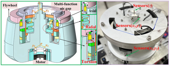
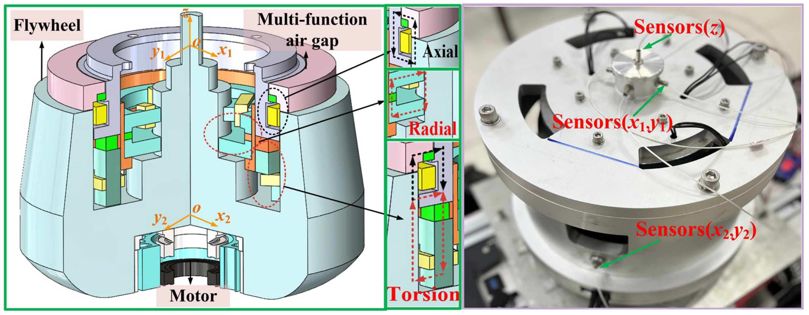
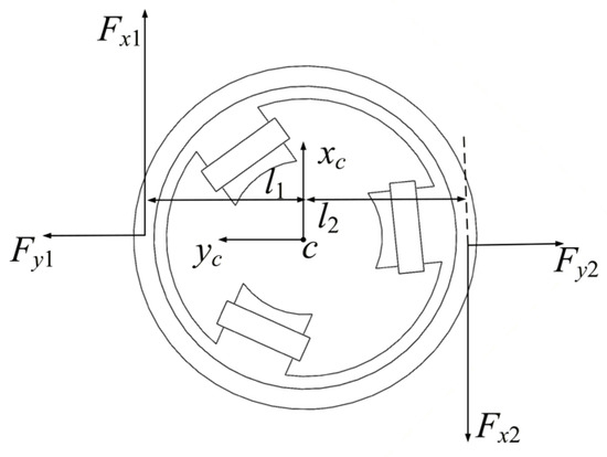
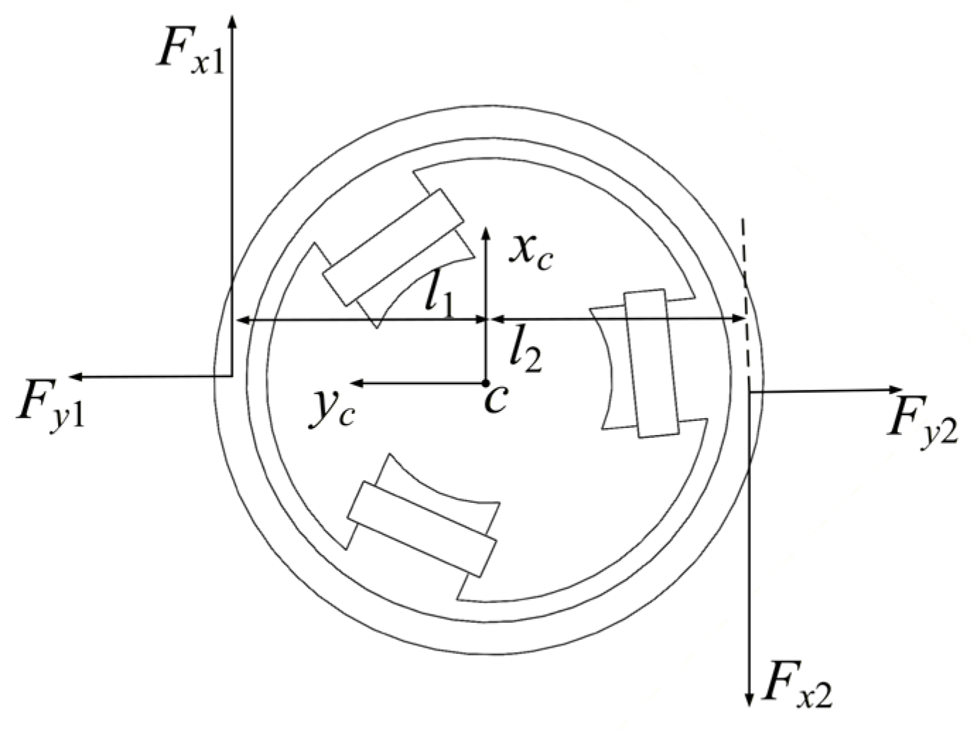
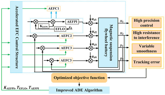
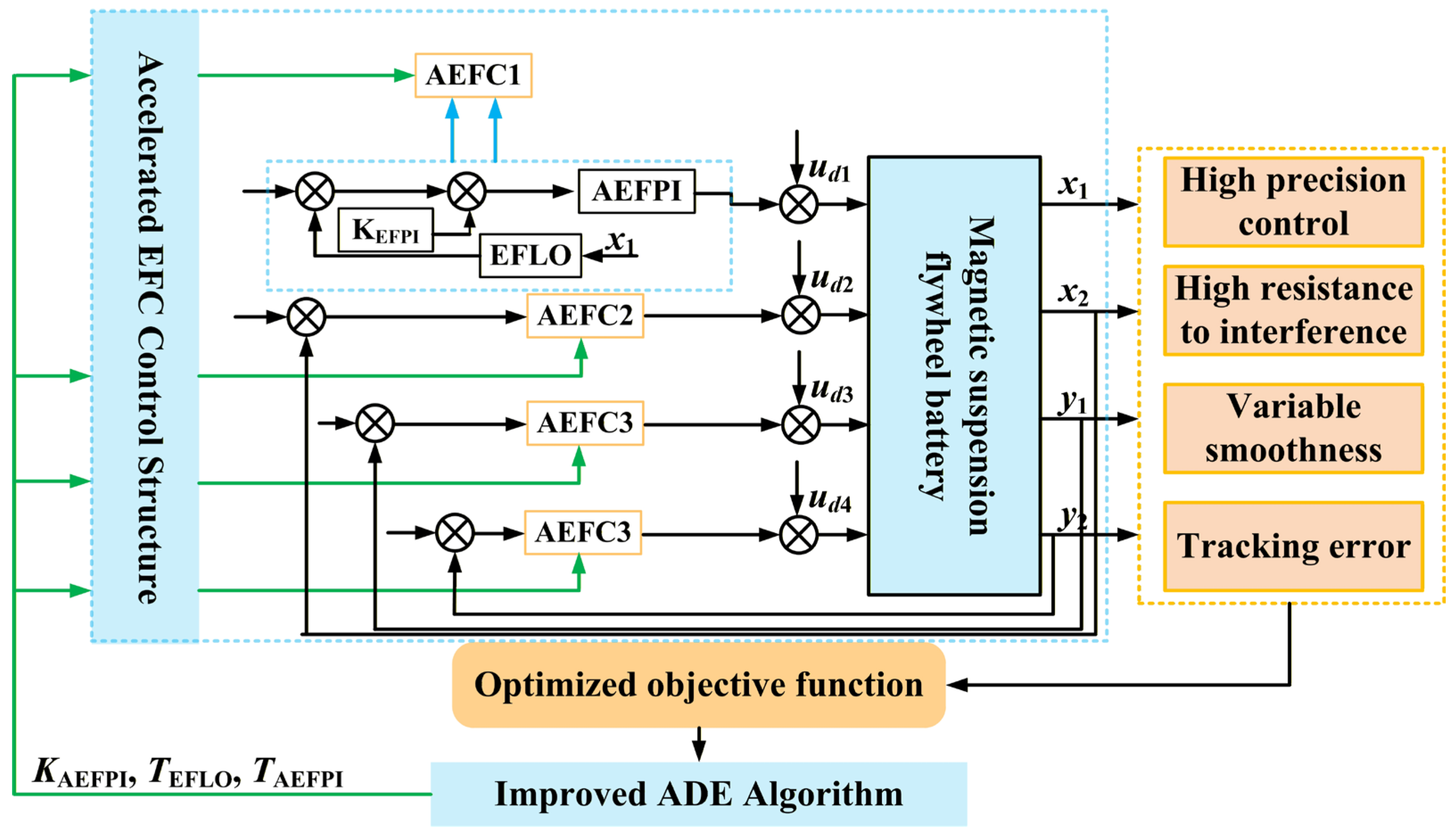
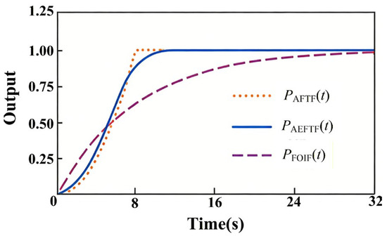
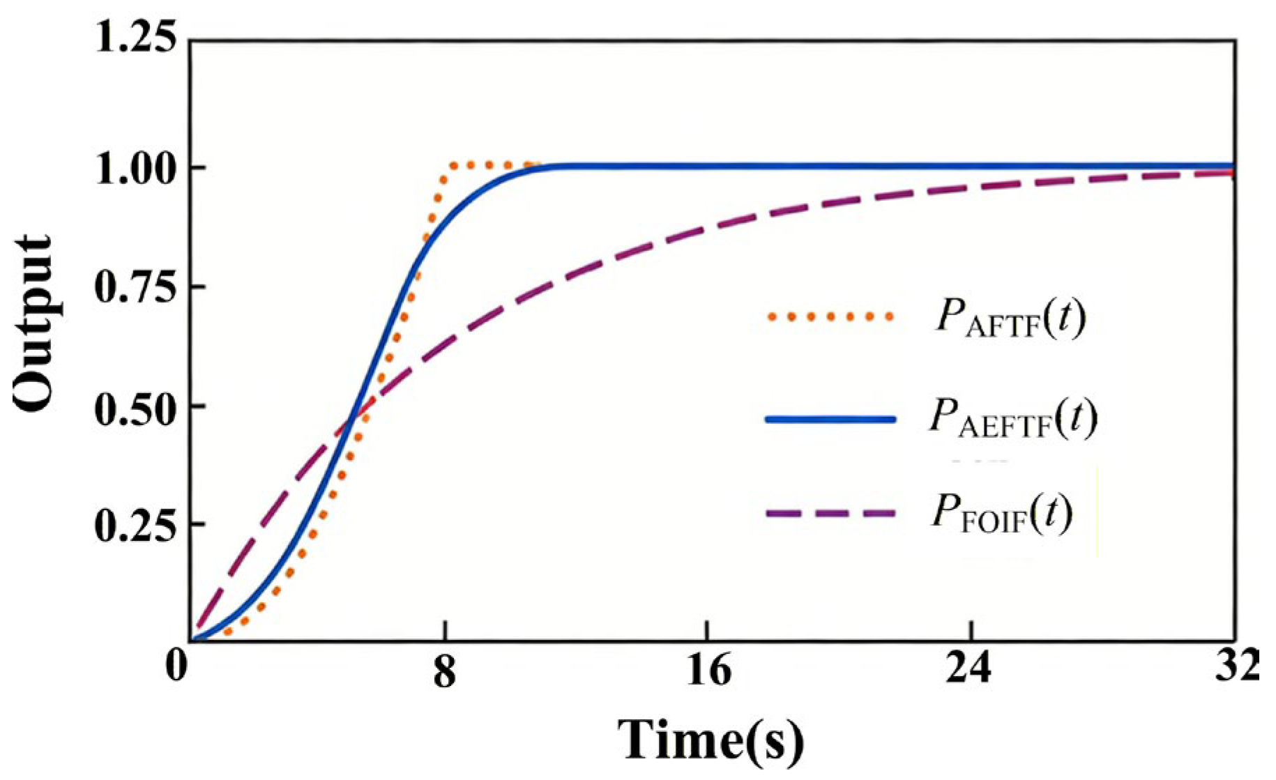
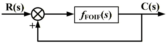
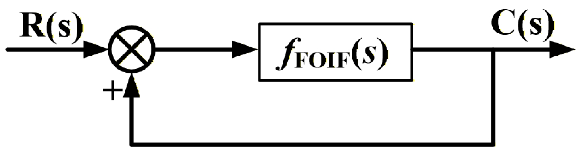
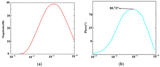
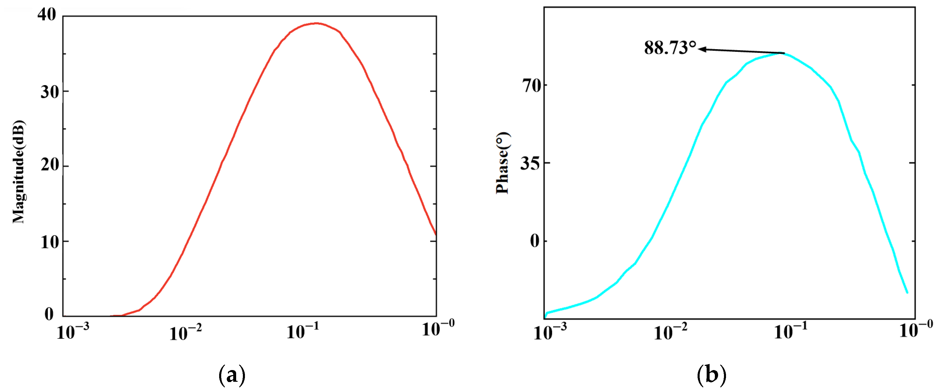
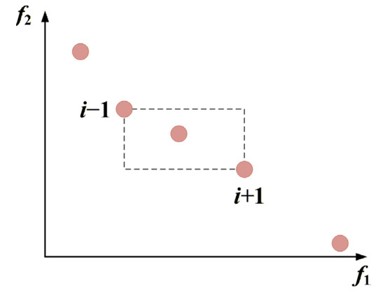
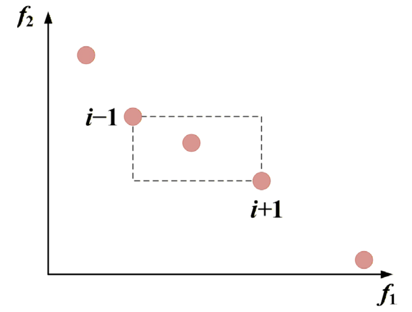
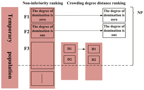
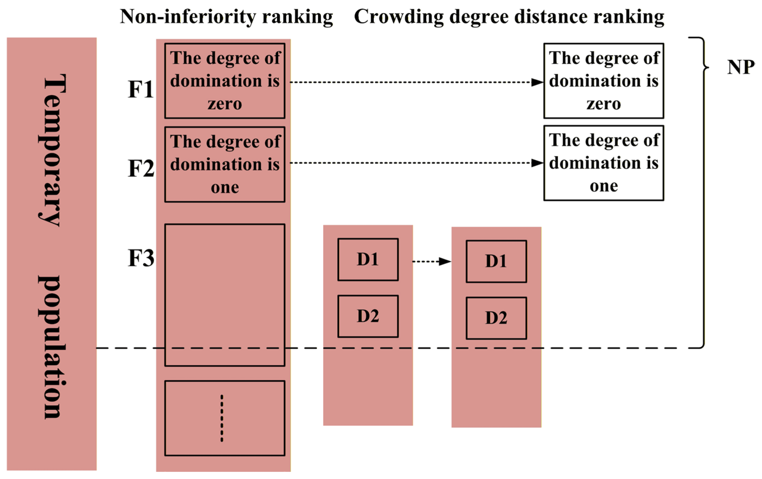
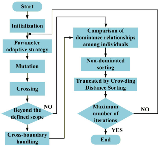
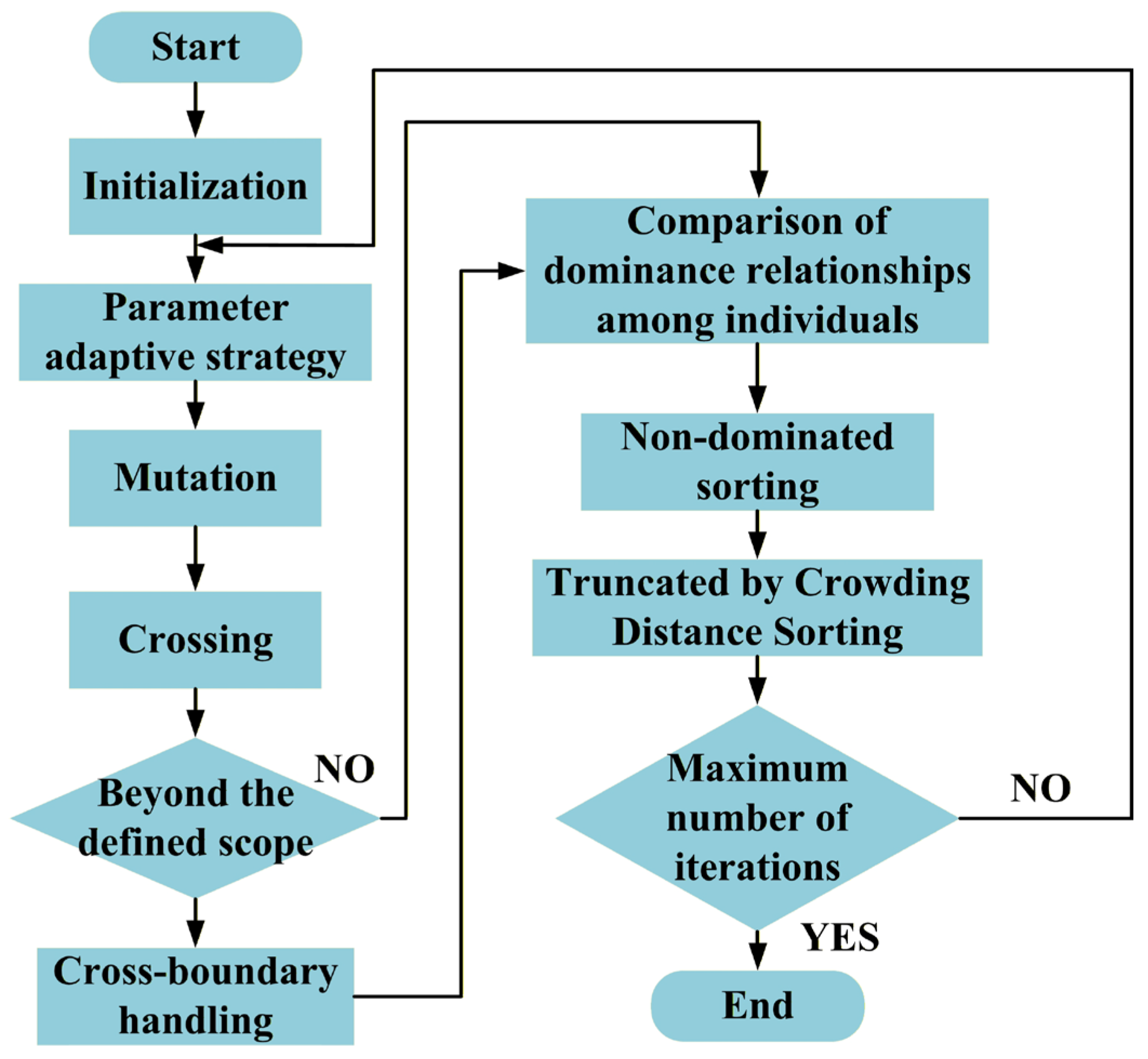
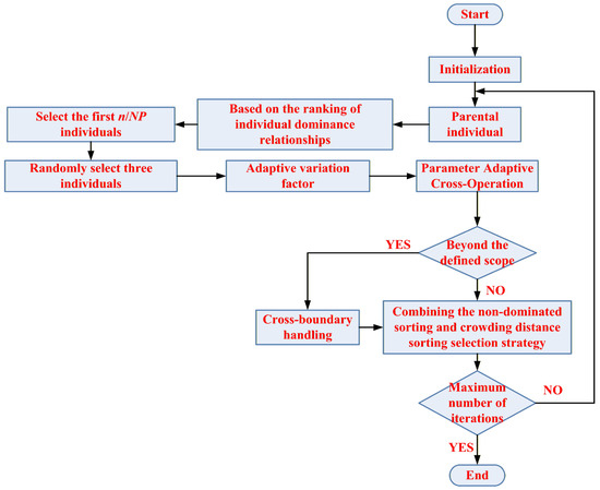
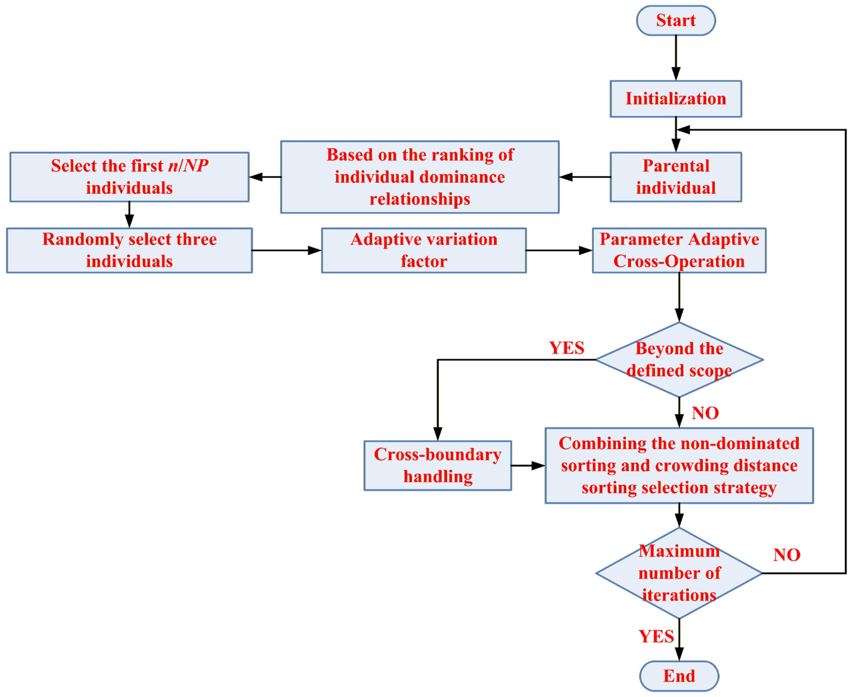
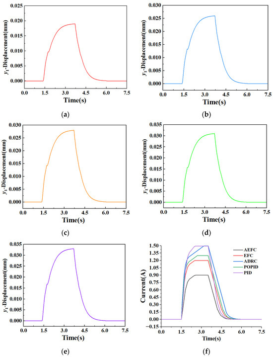
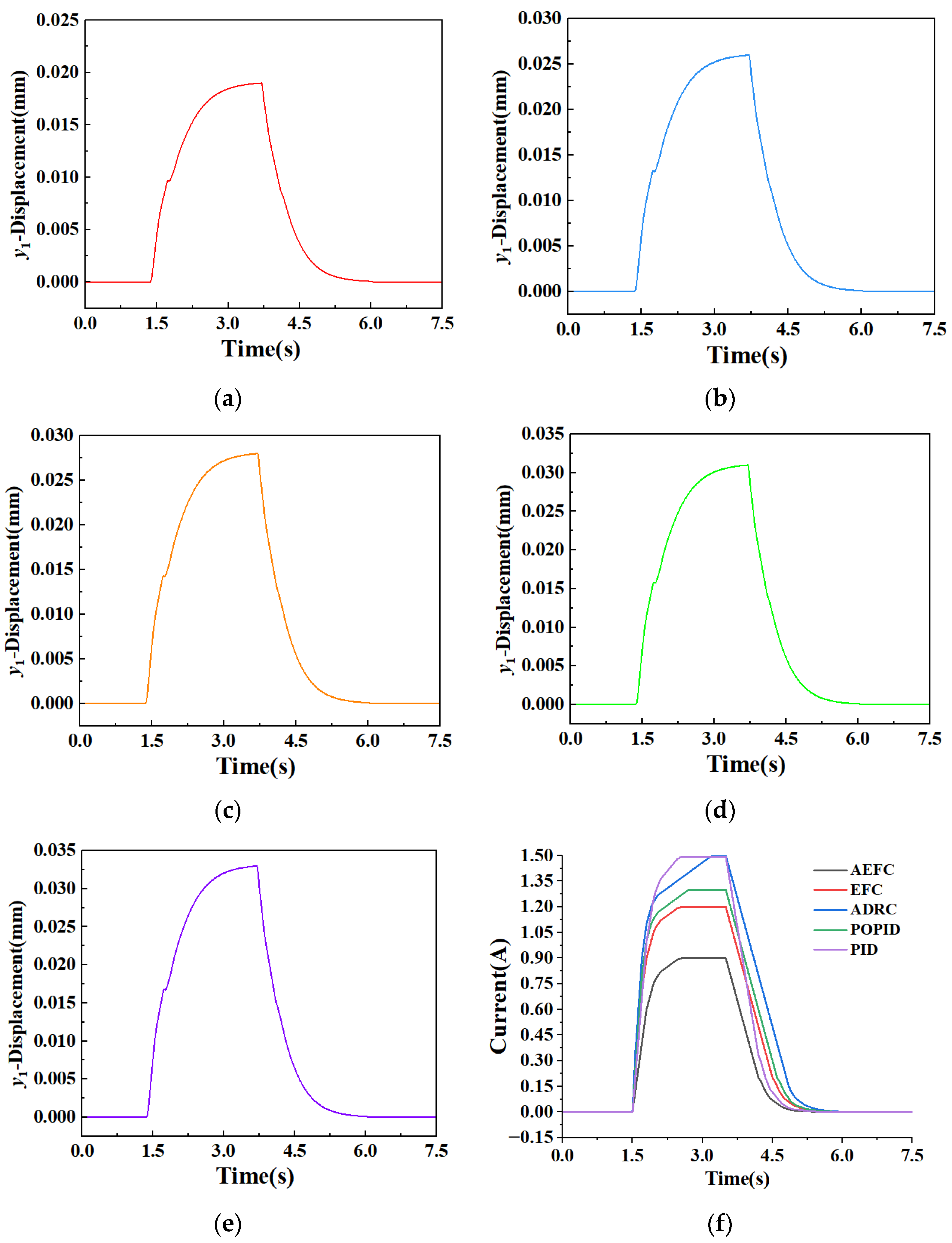
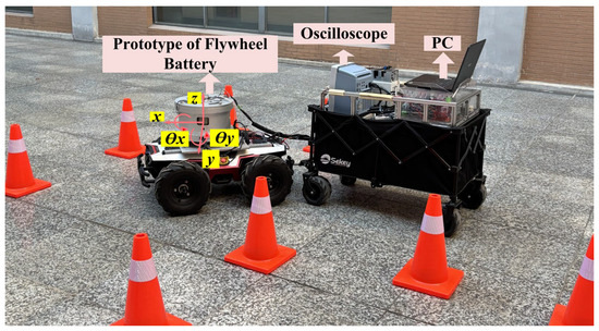
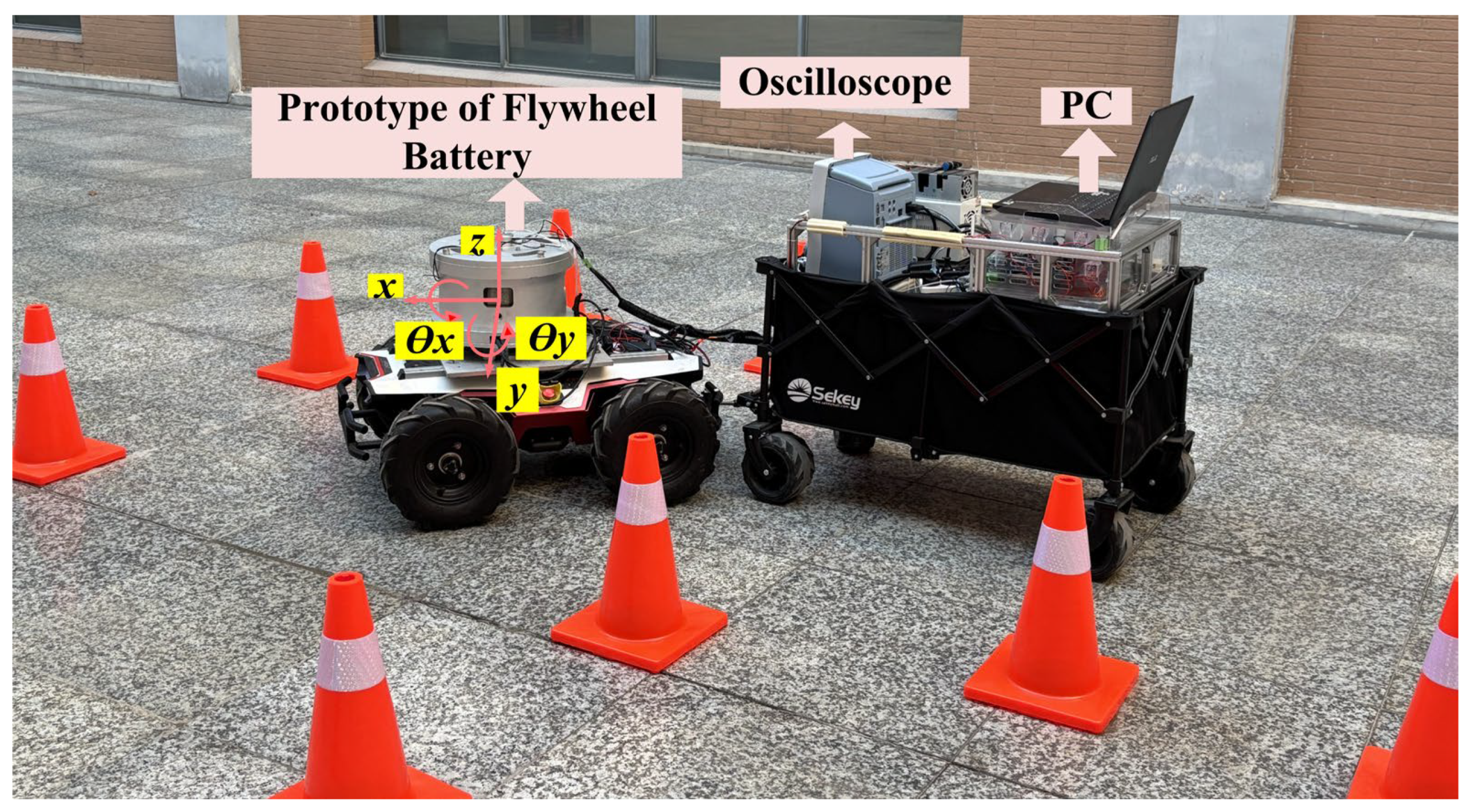
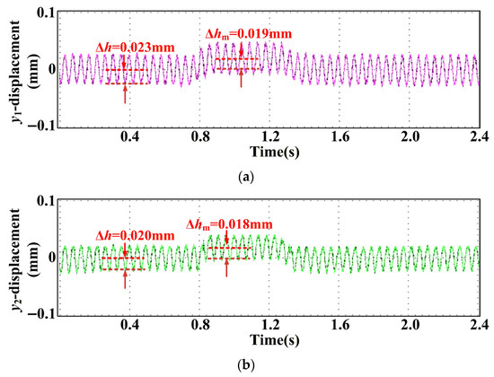
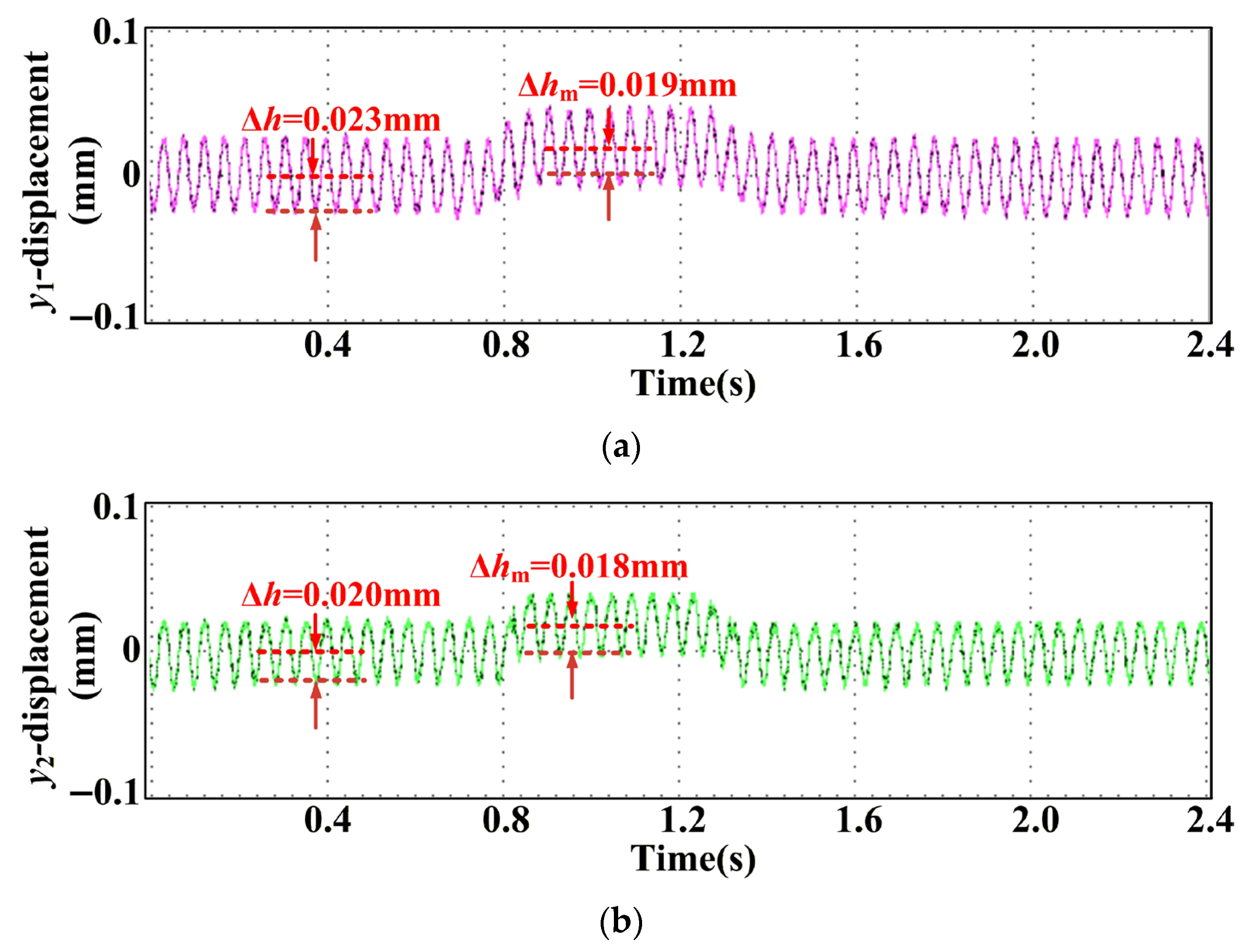
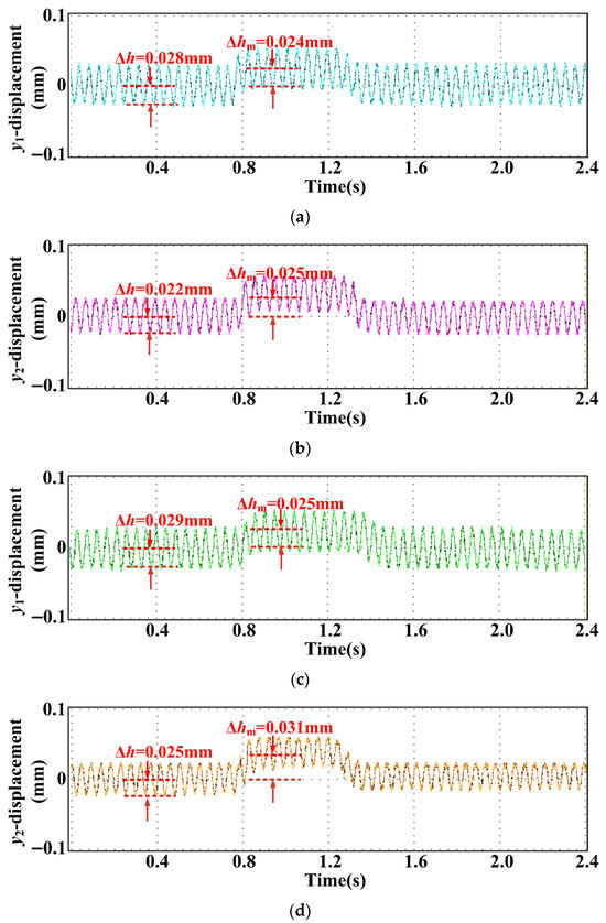
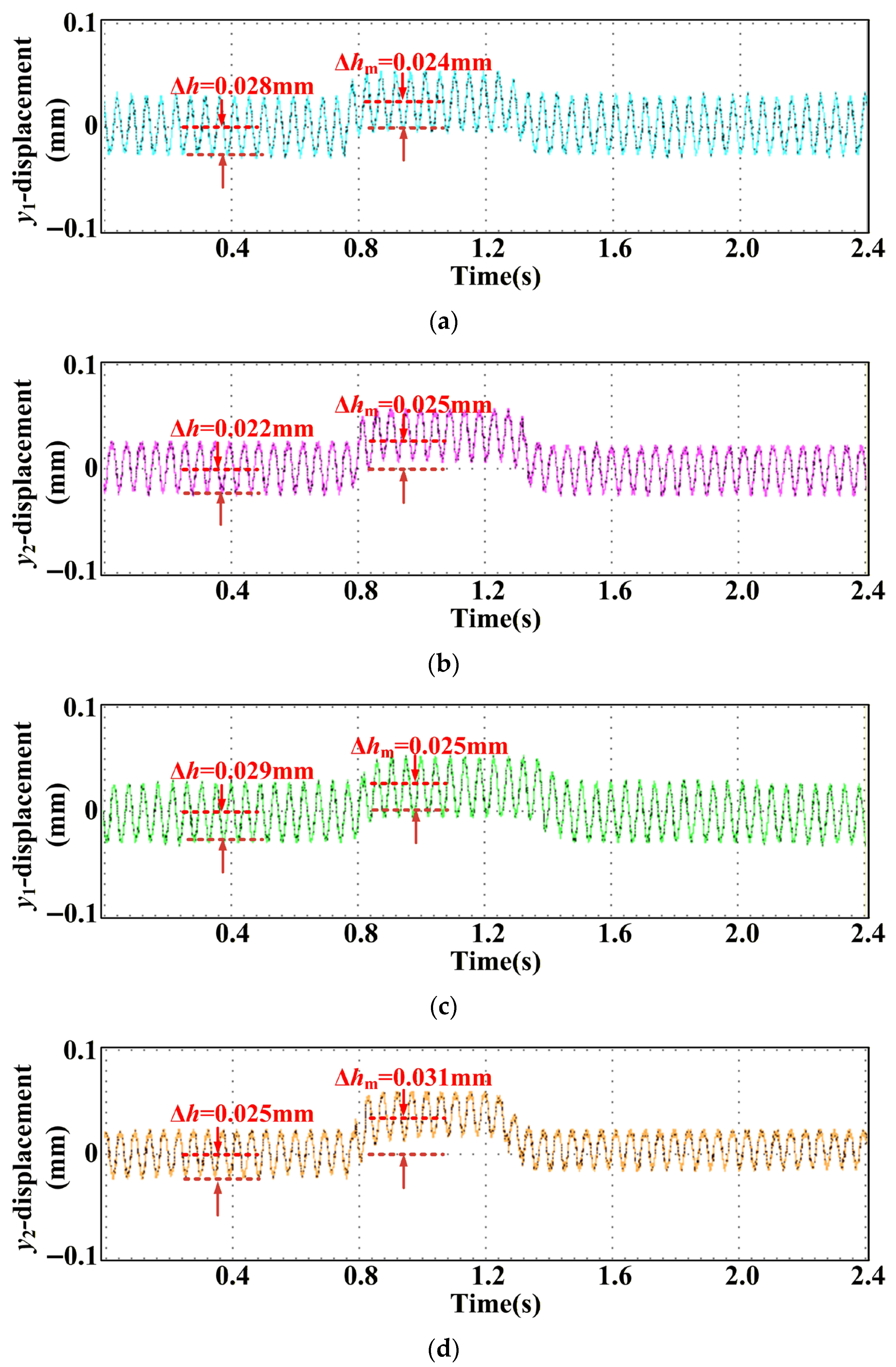
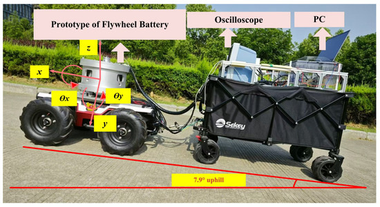
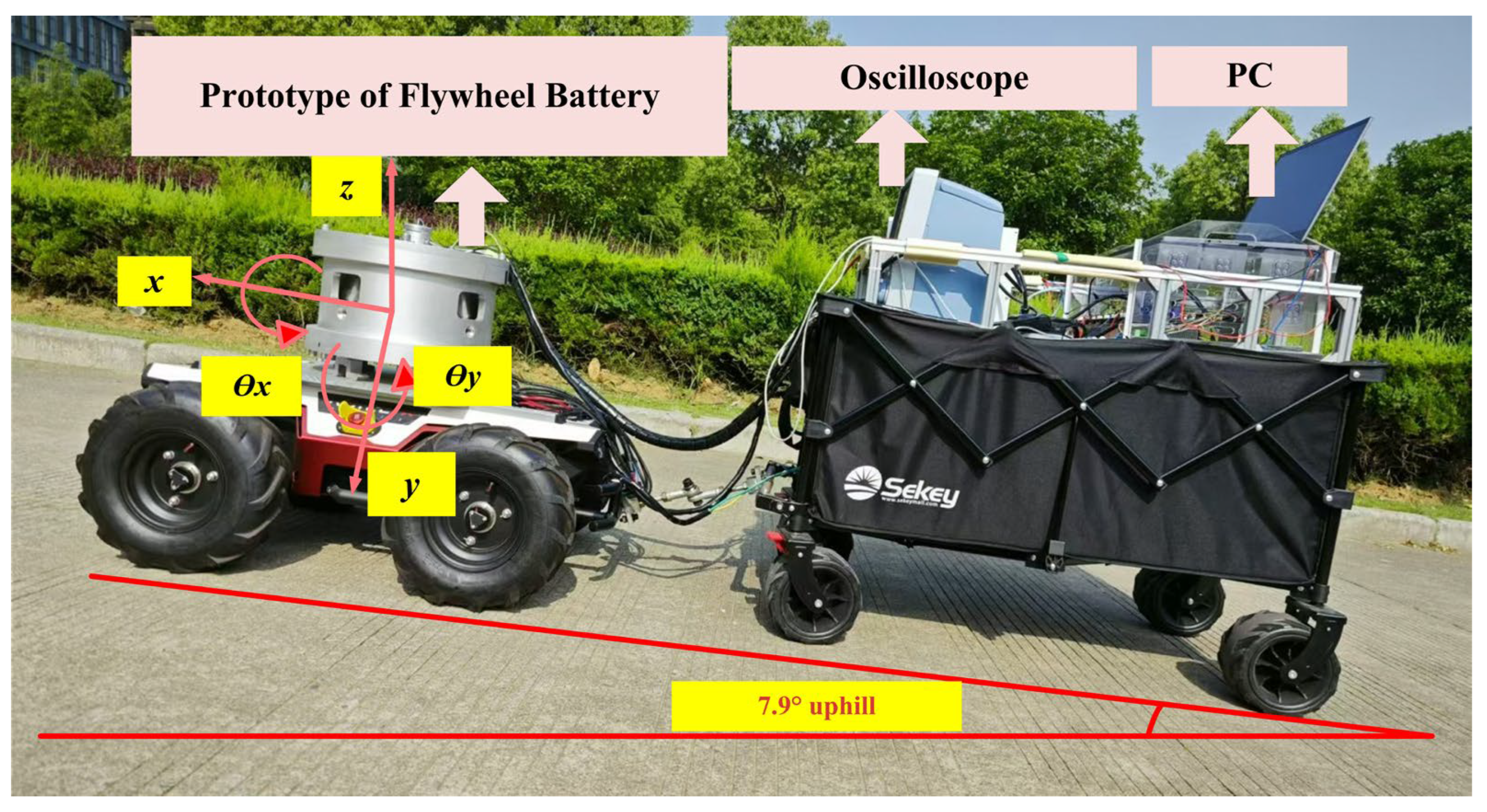
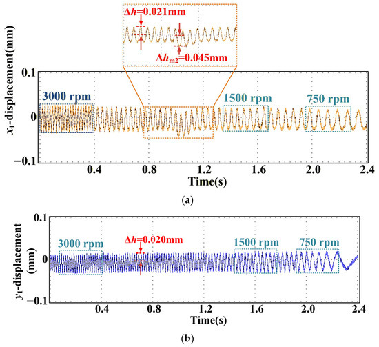
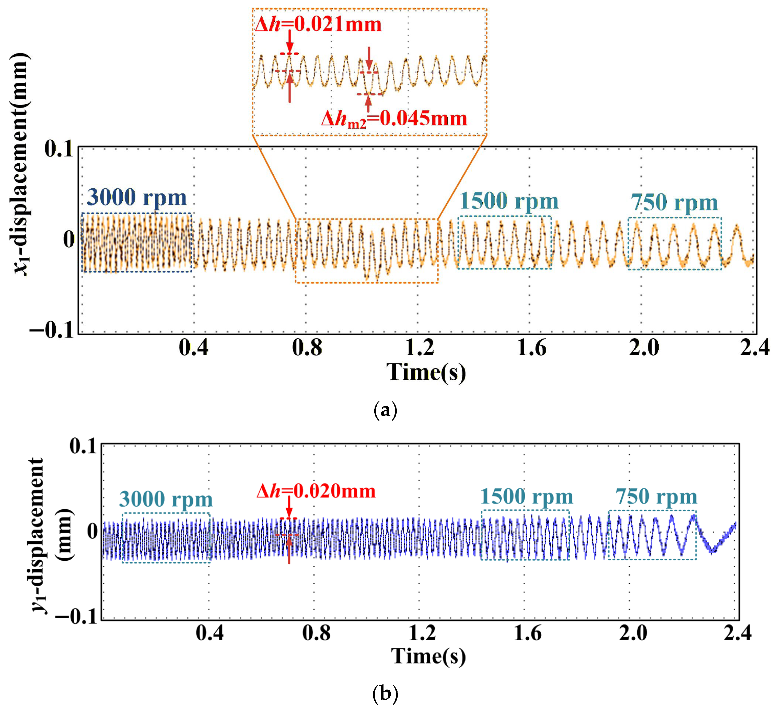
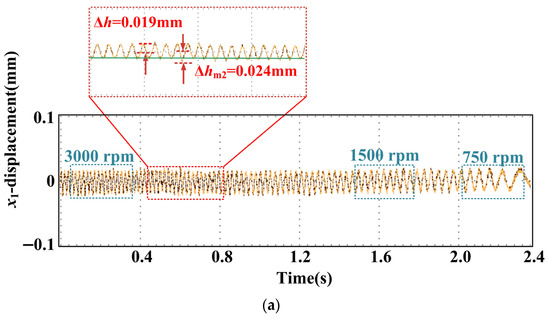
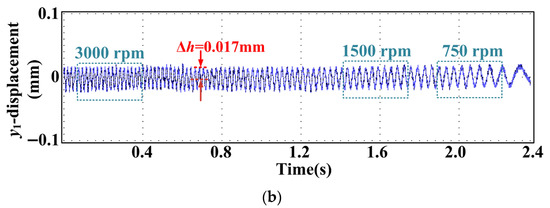
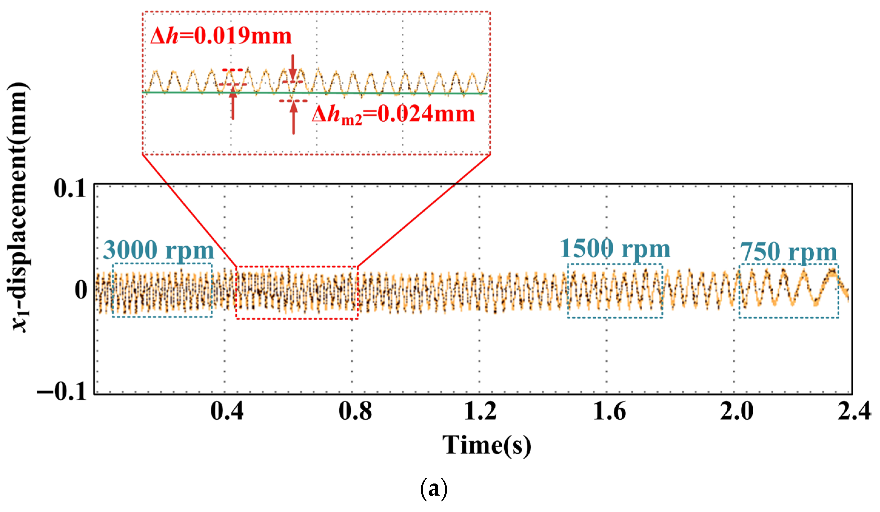
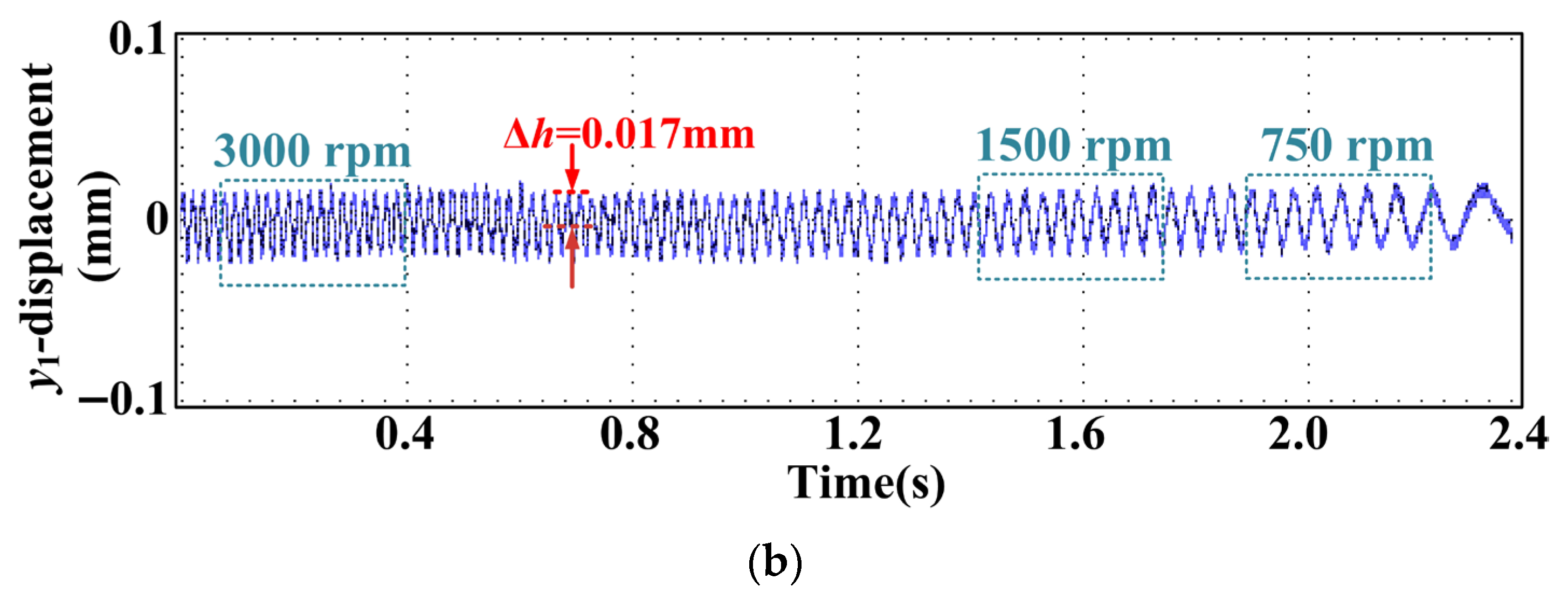

Disclaimer/Publisher’s Note: The statements, opinions and data contained in all publications are solely those of the individual author(s) and contributor(s) and not of MDPI and/or the editor(s). MDPI and/or the editor(s) disclaim responsibility for any injury to people or property resulting from any ideas, methods, instructions or products referred to in the content. |
© 2026 by the authors. Licensee MDPI, Basel, Switzerland. This article is an open access article distributed under the terms and conditions of the Creative Commons Attribution (CC BY) license.