Embedded Delay-Coordinate Predictive Damping for Speed Ripple Attenuation in a Motor–Reducer Flexible Drive

Abstract

Speed ripple attenuation in geared flexible drives requires control of synchronous components and residual fluctuations within an existing embedded control architecture. This paper develops a five-state delay-coordinate predictive damping controller (D5–PD) that adds auxiliary q-axis current to a proportional–integral (PI)-regulated drive. Direction-specific models are identified from drive speed history and auxiliary current records with exact delay shifts. A three-step output-weighted design is solved offline and deployed as five-coefficient feedback with scalar scheduling and current limits, at a 1 ms auxiliary update period on an F28379D. Experiments compare PI, six-branch multi-resonant control (MR), and D5–PD under six conditions with three runs per controller. At +300 r/min and +1 A, D5–PD reduces mean speed ripple root mean square (RMS) by 38.83% relative to PI and 5.61% relative to MR at nearly equal auxiliary command alternating-current (AC) RMS. Its load current-normalized responses at 2 and 8 Hz are 37.39% and 60.17% lower than MR without disturbance-specific retuning. Total ripple is lower than PI in all six conditions and MR in five; residual RMS is lower than MR throughout. A separate 0.20 A benchmark with six records per method gives 2.12% lower total ripple and 7.68% lower command RMS than proportional ripple damping. These results demonstrate an embedded auxiliary damping implementation and characterize its tradeoffs with frequency-selective and proportional feedback in terms of total ripple, residual fluctuations and command demand.

1. Introduction

Speed ripple and transmission vibration impair motion quality in electromechanical drives. In machine tool servo systems, these effects compromise feed uniformity and positioning performance [1,2]; related vibration control problems arise in railway traction and hybrid electric vehicle drivetrains [3,4]. A practical route to improved motion quality is to add damping to a proportional–integral (PI) speed loop [5]. For a geared flexible drive, the challenge is to suppress the measured speed fluctuations while retaining the existing control loops and meeting the computational limits of the motor controller.

Frequency-selective control exploits the periodic structure of disturbances through the internal model principle [6]. For permanent-magnet synchronous motor (PMSM) drives, PI–resonant control [7], adaptive resonant control [8], and equivalent harmonic injection [9] target selected components of the speed ripple. Plug-in repetitive control extends this approach to periodic waveforms [1], with fractional delay compensation and adjustable gain supporting variable-speed operation [10]. These methods provide effective ways to address synchronous ripple. However, suppressing selected orders does not by itself determine the total ripple, which also includes fluctuations outside those components. This distinction motivates a comparison based on both total speed ripple and its synchronous and residual contributions.

Predictive control offers a way to shape the response through a model of the drive dynamics. Cascade PMSM model predictive control (MPC) [11] and predictive–integral–resonant control [12] have been developed for ripple and disturbance attenuation. In flexible drives, predictive designs address shaft-torque limitation through MPC–PI switching [13] and nonlinear vibration dynamics [14], while optimal harmonic current commands provide another route to active torsional vibration suppression [4]. Recent two-mass studies compare analytical MPC with state feedback [15] and incorporate a two-layer observer into predictive control [16]. For the present application, the central design question is how to obtain a predictor from available speed measurements and convert it into auxiliary feedback suitable for embedded execution.

Data-driven prediction provides routes from measured signals to control-oriented models. Koopman-based methods describe observable evolution, with their approximation and control implications reviewed in [17,18,19]. Related modeling tools include extended dynamic mode decomposition [20], dynamic mode decomposition with control [21], and input-dependent operator formulations [22]; finite-dimensional linear predictors support MPC design [23]. Delay-coordinate constructions connect measurement history to spectral analysis and prediction [24,25], including predictive control from sparse measurements [26].

Applications include soft robots and coupled pendulums [27,28], while multiple-model, tube-based, and recurrent formulations address model variation, robustness, and time-delay dynamics [29,30,31]. In electrical drives, reported applications include finite-control-set control [32], predictive current control [33], PMSM velocity control [34], and backward-Koopman-based autoregressive with exogenous input (ARX) predictive control [35]. Comparisons of identified model, subspace, and data-enabled current control [36], together with real-time feasibility studies [37], emphasize the need to connect model identification to implementable feedback.

Inspired by time-delay observable formulations used in Koopman-based prediction [25,26], this study constructs a compact predictor from measured speed error and fluctuation history. With the selected linear coordinates and regression, the resulting predictor admits an equivalent ARX-type realization. The controller is therefore termed five-state delay-coordinate predictive damping (D5–PD). The contribution lies in its direction-specific, output-weighted predictive damping design and embedded experimental implementation for a PI-regulated motor–reducer flexible drive.

Engineering problem and scope. The target is auxiliary damping that can be added to an established PI/current-loop drive using the existing drive speed signal. The design connects a compact identified model to feedback with shared current limits and evaluates selected-order attenuation, residual ripple, and auxiliary command demand. This provides the basis for assessing the complete embedded implementation alongside frequency-selective and proportional damping.

The implementation is denoted D5–PD; D5 refers to its five-state predictor. Three engineering contributions are developed:

• A measurement-based design path identifies the PI-regulated auxiliary current-to-speed response separately for each direction. The five-state representation combines tracking error and speed-fluctuation history, fits only two dynamic rows, and preserves exact delay shifts. Its synthesis uses the existing drive speed signal and auxiliary current record, without requiring identified shaft stiffness or load-side motion in the feedback law.
• An offline-to-embedded realization converts the three-step, two-output quadratic design into one fixed five-coefficient row per direction. The resulting auxiliary branch retains the PI and inner current loops and interfaces with deployment scaling, speed scheduling, activation logic, and common current limits. Supplementary Section S10 complements this implementation with hardware measurements of the control-function and auxiliary-update intervals.
• An experimental evaluation characterizes the measured tradeoff between selected-order suppression, residual ripple, and command demand. The original six-condition campaign includes reverse rotation, load variation, higher speed, and two disturbances away from the multi-resonant (MR) centers with unchanged controller settings. A separate reduced-load proportional-damping benchmark tests whether the measured benefit extends beyond frequency-selective compensation.

2. Experimental System and Control Structure

2.1. Drive System and Measured Signals

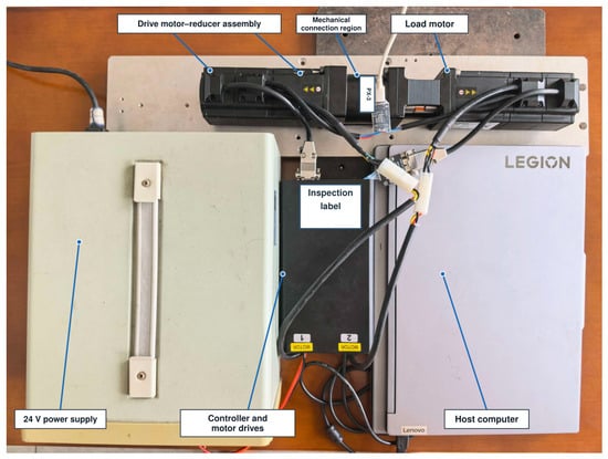
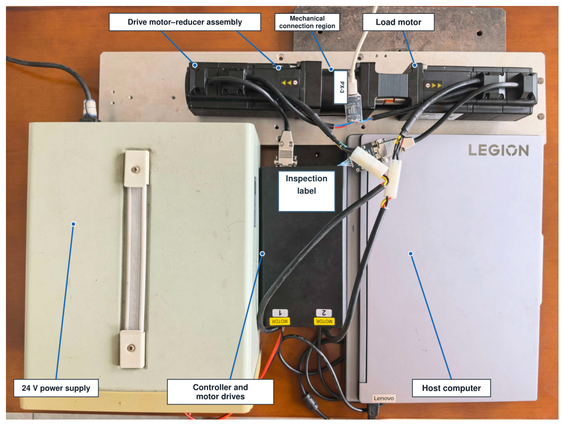
The experimental platform comprises a drive PMSM connected to a load PMSM through a reducer and flexible coupling, as shown in Figure 1. Both motor drives operate from a 24-V supply. The controller runs in single precision on an F28379D processor, and a host computer records the experimental signals. The nominal reducer ratio used by the controller is $i_g=3.25$.

Figure 1. Motor–reducer experimental platform. The mechanical path connects the drive motor, reducer, coupling, and load motor.

The base control period is $T_b=100\mathsf{\mu }$s, while the auxiliary controller updates every $T_a=1$ ms. Each motor has a configured encoder resolution of 2500 lines. The drive speed signal supplied by the existing motor control software is used for both feedback and performance evaluation. Motor and inverter settings are listed in Supplementary Material, Section S5.

The recorded signals comprise drive speed, measured drive current, the auxiliary current command after limiting, measured load-motor current, and controller and limiter states. Speed is converted from per unit using a 3000 r/min base. Drive current fluctuations quantify current ripple, and the applied auxiliary command quantifies control effort. Measured load current is used to normalize the imposed disturbance response. Controller state records identify the active analysis interval and the operation of the current limits.

Let ${\theta }_d$ and ${\theta }_l$ denote the mechanical positions of the drive and load motors. With an output-side sign convention,

$$\begin{array}{c}{\theta }_o={\theta }_d/i_g,{\omega }_o={\omega }_d/i_g,\\ {\theta }_{\mathrm{\Delta }}={\theta }_o-{\theta }_l,{\omega }_{\mathrm{\Delta }}={\omega }_o-{\omega }_l.\end{array}$$

(1)

Here, ${\omega }_d={\dot{\theta }}_d$ and ${\omega }_l={\dot{\theta }}_l$. The flexible path has the two-inertia representation

$$\begin{array}{cc}\hfill J_{do}{\dot{\omega }}_o& =T_{eo}-T_s-B_{do}{\omega }_o,\hfill \end{array}$$

(2)

$$\begin{array}{cc}\hfill J_l{\dot{\omega }}_l& =T_s-T_L-B_l{\omega }_l,\hfill \end{array}$$

(3)

$$\begin{array}{cc}\hfill T_s& =K_s{\theta }_{\mathrm{\Delta }}+C_s{\omega }_{\mathrm{\Delta }}.\hfill \end{array}$$

(4)

Here, $J_{do}$, $B_{do}$, and $T_{eo}$ denote the drive-side inertia, viscous friction, and applied torque referred to the reducer output. The corresponding load-side quantities are $J_l$, $B_l$, and $T_L$. The transmitted torque $T_s$ depends on the relative displacement and velocity through the equivalent stiffness $K_s$ and damping $C_s$. Equations (2)–(4) describe the mechanical coupling; the controller developed below instead obtains its predictive model directly from measured drive speed and auxiliary current commands.

2.2. Common PI and Auxiliary Current Paths

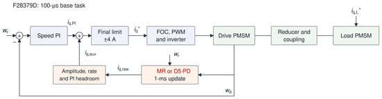
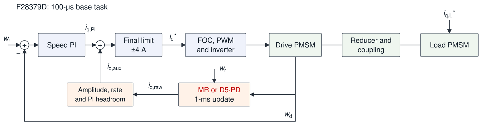
Figure 2 shows the control structure. Let ℓ denote the base-task index and k the auxiliary-task index. Speeds $w_d$ and $w_r$ are expressed in per unit on $n_b=3000$ r/min, with $n_r=n_b{w}_r$ the ramped reference in r/min. The PI error is $e_{\mathrm{PI}}=w_r-w_d$. The implemented PI output is

$$\begin{array}{c}{i}_{q,\mathrm{PI}}\left(\mathcal{l}\right)={\mathrm{sat}}_{[-4,4]}\left(K_p{e}_{\mathrm{PI}}\left(\mathcal{l}\right)+K_i\xi \left(\mathcal{l}\right)\right),\\ K_p=7,K_i=50.\end{array}$$

(5)

Figure 2. Speed control structure. MR or D5–PD supplies the auxiliary current; the load motor applies the programmed load and disturbance.

Here, ${\mathrm{sat}}_{[a,b]}\left(x\right)=\min \{b,\max \{a,x\}\}$ denotes scalar saturation to the interval $[a,b]$. The integral state $\xi$ is bounded by $4/K_i$ in magnitude. Its candidate update is accepted when the unsaturated PI output lies within the current limits or the error drives it back toward the admissible range. The final current command is

$$\begin{array}{c}{i}_q^{★}\left(\mathcal{l}\right)={\mathrm{sat}}_{[-4,4]}\left(i_{q,\mathrm{PI}}\left(\mathcal{l}\right)+i_{q,\mathrm{aux}}\left(k\left(\mathcal{l}\right)\right)\right),\\ k\left(\mathcal{l}\right)=\lfloor \mathcal{l}/10\rfloor .\end{array}$$

(6)

The auxiliary command is held constant between successive 1 ms updates. For the PI baseline, $i_{q,\mathrm{aux}}=0$. In the original auxiliary configurations, either MR or D5–PD generates this command, subject to identical amplitude, rate, and PI current headroom limits.

2.3. Synchronous Orders and the MR Controller

The first three output-side and drive-side mechanical-order frequencies are

$$f_{o,m}={\displaystyle \frac{m|n_r|}{60i_g}},f_{d,m}={\displaystyle \frac{m|n_r|}{60}},m=1,2,3.$$

(7)

At $|n_r|=300$ r/min, the six centers are

$${\mathcal{F}}_s=\{1.5385,3.0769,4.6154,5,10,15\}\mathrm{Hz}.$$

(8)

Each branch uses the continuous resonant prototype

$$\begin{array}{c}{G}_{R,j}\left(s\right)={\displaystyle \frac{2{\omega }_{b}s}{s^2+2{\omega }_{b}s+{\mathrm{\Omega }}_{0,j}^2}},\\ {\omega }_b=2\pi \left(0.18\mathrm{Hz}\right),{\mathrm{\Omega }}_{0,j}=2\pi f_{R,j}.\end{array}$$

(9)

The parameter ${\omega }_b$ sets the resonant damping/bandwidth, and $f_{R,j}$ and ${\mathrm{\Omega }}_{0,j}$ are the scheduled center frequency and its angular frequency. Each filter is discretized at 1 ms with center frequency prewarping and implemented in transposed direct form II. The input is $-w_{\mathrm{ac},k}$, where $w_{\mathrm{ac},k}$ is the speed fluctuation defined in Equation (13). The six filter outputs are summed and multiplied by a common gain of 20 A/pu. This controller serves as the frequency-selective benchmark, following the resonant control principle in [7,8]. Its centers track the reference speed through Equation (7), while the common gain and bandwidth remain unchanged across all reported conditions. The discrete coefficients are given in Supplementary Material, Section S2.

Conventional damping comparator. The reduced-load supplementary study additionally evaluates proportional speed ripple damping (SD), with pre-limit command

$${\widehat{i}}_{q,\mathrm{SD}}\left(k\right)=-13w_{\mathrm{ac},k}\left[\mathrm{A}\right].$$

(10)

The fluctuation is in per unit and the coefficient has units A/pu. SD retains the PI speed loop and shares the auxiliary amplitude, rate and PI-headroom limits. Its gain is fixed within the six-record benchmark.

3. Delay-Coordinate Predictive Controller

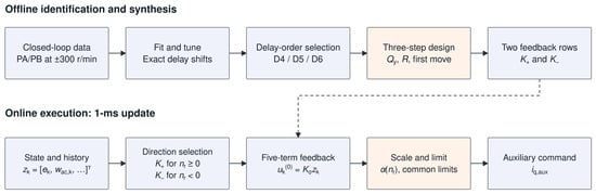
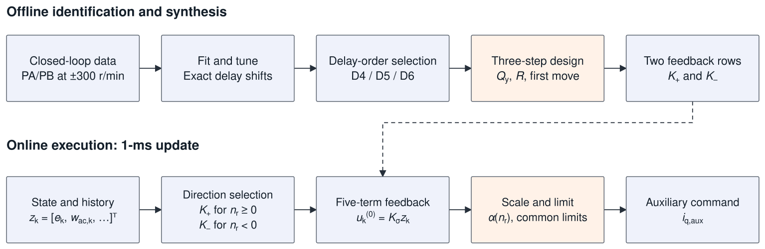
The proposed controller is constructed in three stages: identification of a structured delay-coordinate predictor, offline synthesis of predictive feedback, and online evaluation of the resulting fixed-gain law. Figure 3 summarizes this process.

Figure 3. Identification and deployment of D5–PD. Fitting and tuning determine the predictor; the three-step design gives two feedback rows for online execution. Signed-load records are reserved for prediction evaluation. The dashed arrow indicates transfer of the offline-designed feedback gains to the online controller.

3.1. Closed-Loop Identification Records

Separate models are identified at +300 and −300 r/min with the speed PI loop active. Each model therefore describes the response of the PI-regulated drive to auxiliary current commands. Two zero-load records with different excitation phases are used for training in each direction; a loaded record is reserved for independent prediction evaluation. For positive rotation, the training records are P300_0A_PA_R01 and P300_0A_PB_R01, and the held-out record is P300_1A_PB_R01. The negative direction model uses the corresponding N300_0A_PA/PB records for training and N300_N1A_PB_R01 for evaluation.

The excitation is a deterministic multisine with frequencies

$${\mathcal{F}}_{\mathrm{ID}}=\{1.3,2.4,4.0,6.4,9.1,13.7\}\mathrm{Hz}.$$

(11)

In Equation (12), t is measured from excitation onset, and $f_{\mathrm{ID},j}$ and ${\varphi }_j$ denote the frequency and phase of the jth identification tone, respectively. The amplitude parameter is 0.025 A, and the tone weights are $\eta =[1.00,0.90,0.80,0.70,0.55,0.40]$. During the constant-envelope portion, the requested excitation is

$$i_{q,\mathrm{ID}}\left(t\right)={\displaystyle \frac{0.025}{{\sum }_{j=1}^6{\eta }_j}}{\displaystyle \sum _{j=1}^6}{\eta }_j\sin (2\pi f_{\mathrm{ID},j}t+{\varphi }_j).$$

(12)

The PA phase vector is $[0.20,0.75,1.10,1.65,2.20,2.75]$ rad, and PB shifts every component by $\pi /2$. Excitation is applied for 12 s, including 1 s linear ramps at the beginning and end. Excluding the ramps leaves a 10 s identification interval. The recorded auxiliary command after limiting is used as the model input.

Signal quality processing is detailed in Supplementary Material, Section S6.

Every tenth processed acquisition sample is retained to obtain the 1 ms sequence used for modeling. The slow-speed filter is initialized by processing the preceding samples in each record before the identification interval begins. Each training record is divided chronologically into 70% for fitting and 30% for tuning. The loaded records remain separate throughout parameter and model-order selection.

3.2. Structured Delay State and Model Fitting

The predictor is identified directly in linear measurement history coordinates. It approximates the response of the drive with the existing PI loop active, using auxiliary current as its input and measured speed error and fluctuation as its two dynamic outputs. Delayed fluctuation samples retain recent history through exact register shifts.

At each auxiliary update, the measured speed is separated into a slowly varying component and an alternating component (AC):

$$\begin{array}{c}{\overline{w}}_{d,k}={\overline{w}}_{d,k-1}+a_{\mathrm{dc}}(w_{d,k}-{\overline{w}}_{d,k-1}),\\ w_{\mathrm{ac},k}=w_{d,k}-{\overline{w}}_{d,k},a_{\mathrm{dc}}=0.003139715.\end{array}$$

(13)

The predictive control error uses the opposite sign to the PI error:

$$e_k=w_{d,k}-w_{r,k}=-e_{\mathrm{PI},k}.$$

(14)

The prediction state combines this error with the current AC speed value and its three most recent samples:

$$z_k={\left[\begin{array}{ccccc}{e}_k& w_{\mathrm{ac},k}& w_{\mathrm{ac},k-1}& w_{\mathrm{ac},k-2}& w_{\mathrm{ac},k-3}\end{array}\right]}^{\top }.$$

(15)

Retaining $e_k$ allows tracking error and AC speed to receive separate weights while PI regulates mean speed. For a known reference, the maintained slow-speed estimate satisfies ${\overline{w}}_{d,k}=w_{r,k}+e_k-w_{\mathrm{ac},k}$ and is recoverable from these coordinates. For direction $\sigma \in \{+,-\}$, its dynamics are approximated by

$$z_{k+1}=A_{\sigma }{z}_k+B_{\sigma }{u}_k+{\epsilon }_{\sigma ,k},$$

(16)

where $u_k$ is the recorded auxiliary command after subtraction of its record mean, expressed in amperes, and the state entries are in per unit. The residual ${\epsilon }_{\sigma ,k}$ represents the model error and is set to zero when generating predictions.

With these linear delay coordinates, Equation (16) is a linear model in measurement history coordinates. The shift rows implement exact register updates; the first two rows approximate the dynamics of the two measured outputs. Only the evolution of speed error and the current AC speed value must be identified, so regression is restricted to the first two rows of $\left[A_{\sigma }{B}_{\sigma }\right]$. The remaining states shift the measured history by one sample and satisfy

$$\begin{array}{c}{A}_{\sigma }(3,2)=A_{\sigma }(4,3)=A_{\sigma }(5,4)=1,\\ B_{\sigma }(3:5)=0.\end{array}$$

(17)

All other entries in the last three rows of $A_{\sigma }$ are zero. These shifts are exact, so the corresponding entries of ${\epsilon }_{\sigma ,k}$ are also zero.

Let N denote the number of aligned state transitions. Let $Z,Z^{+}\in {\mathbb{R}}^{5\times N}$ contain the present and successor states, and let $U\in {\mathbb{R}}^{1\times N}$ contain the corresponding inputs. With $S_z=\mathrm{diag}(s_1,\dots ,s_5)$ and $S_u=s_u$ formed from sample standard deviations of the fitting data, define

$$\begin{array}{c}\tilde{Z}=S_z^{-1}Z,{\tilde{Z}}^{+}=S_z^{-1}{Z}^{+},\\ \tilde{U}=S_u^{-1}U,\tilde{X}=\left[\begin{array}{c}\tilde{Z}\\ \tilde{U}\end{array}\right].\end{array}$$

(18)

With ridge regularization parameter $\lambda$ and the $6\times 6$ identity matrix $I_6$, the two unknown normalized rows are obtained by ridge regression:

$${\tilde{\mathrm{\Theta }}}_{\sigma ,1:2}={\tilde{Z}}_{1:2,:}^{+}{\tilde{X}}^{\top }{\left(\tilde{X}{\tilde{X}}^{\top }+\lambda I_6\right)}^{-1}.$$

(19)

The fitted matrix ${\tilde{\mathrm{\Theta }}}_{\sigma ,1:2}$ is $2\times 6$, giving twelve estimated coefficients per direction. Partitioning it as $\left[{\tilde{A}}_{\sigma ,1:2,:}{\tilde{B}}_{\sigma ,1:2,:}\right]$ and reversing the normalization yields

$$\begin{array}{cc}\hfill A_{\sigma ,1:2,:}& =S_{z,12}{\tilde{A}}_{\sigma ,1:2,:}{S}_z^{-1},\hfill \\ \hfill B_{\sigma ,1:2,:}& =S_{z,12}{\tilde{B}}_{\sigma ,1:2,:}{S}_u^{-1}.\hfill \end{array}$$

(20)

Here, $S_{z,12}=\mathrm{diag}(s_1,s_2)$. The exact delay rows are then appended using Equation (17).

Measurement and filtering errors in the regressors, together with closed-loop PI correlations, can bias the fitted coefficients. Ridge regularization improves conditioning but generally retains this errors-in-variables bias. The matrices are assessed as empirical predictors on held-out loaded records.

The regularization parameter is selected from nine logarithmically spaced values between ${10}^{-3}$ and ${10}^1$. The tuning score averages the one- and three-step variance accounted for (VAF) values for both speed error and AC speed. Candidates must also satisfy the checks in Supplementary Material, Section S6. Both five-state models select $\lambda =1$. The model and normalization scales are then refitted using the two complete training records for the corresponding direction.

The model in Equation (16) is an ARX-type linear delay-coordinate realization. Its matched ARX representation is algebraically equivalent; the numerical reconstruction in Section 5.1 is a consistency check rather than a comparison against an independent method.

3.3. Delay-Order Selection

The candidate models D4, D5, and D6 combine speed error with three, four, and five AC speed samples, respectively. They are compared over the same aligned data interval, with the first three transitions of the preliminary state sequence removed to provide the history required by D6. Model order is selected using the three-step AC speed tuning VAF averaged over both directions. The smallest model within 0.50 percentage point of the best score is retained, balancing predictive accuracy against state dimension.

As shown in Table 1, D5 is 0.299 percentage point below D6, whereas D4 is 0.687 percentage point below it. D5 is therefore the smallest candidate that satisfies the specified accuracy tolerance.

Table 1. Delay-order selection: three-step alternating-component (AC) speed tuning variance accounted for (VAF).

Model	Positive (%)	Negative (%)	Mean (%)
D4	77.563	70.042	73.802
D5	77.724	70.656	74.190
D6	77.881	71.098	74.489

3.4. Output-Weighted Predictive Feedback

The two performance outputs are speed error and the AC speed fluctuation:

$$\begin{array}{c}{y}_k=C_y{z}_k={\left[\begin{array}{cc}{e}_k& w_{\mathrm{ac},k}\end{array}\right]}^{\top },\\ C_y=\left[\begin{array}{cc}{I}_2& 0_{2\times 3}\end{array}\right].\end{array}$$

(21)

For the identified linear model, let $y_{k+j|k}$ denote the predicted output and $u_{k+j|k}$ the planned input for time $k+j$, computed at k. The three-step cost is

$$\begin{array}{c}{J}_k={\displaystyle \sum _{j=1}^3}{y}_{k+j|k}^{\top }{Q}_y{y}_{k+j|k}+{\displaystyle \sum _{j=0}^2}R{u}_{k+j|k}^2,\\ Q_y=\mathrm{diag}(2\times {10}^4,6\times {10}^6),R=300.\end{array}$$

(22)

The AC speed weight is 300 times the tracking error weight, emphasizing ripple attenuation while the PI loop regulates mean speed. The input penalty controls the requested auxiliary current magnitude in the unconstrained predictive design. Hard amplitude and rate limits are imposed separately during execution, as specified in Equations (30) and (31). The weights and prediction horizon are identical for both directions.

Stack the predicted outputs and inputs as

$$\begin{array}{cc}\hfill Y_k& ={[y_{k+1|k}^{\top },y_{k+2|k}^{\top },y_{k+3|k}^{\top }]}^{\top },\hfill \\ \hfill U_k& ={[u_{k|k},u_{k+1|k},u_{k+2|k}]}^{\top }.\hfill \end{array}$$

Repeated substitution of Equation (16) gives

$$Y_k=F_{\sigma }{z}_k+G_{\sigma }{U}_k,$$

(23)

where

$$\begin{array}{c}{F}_{\sigma }=\left[\begin{array}{c}{C}_y{A}_{\sigma }\\ C_y{A}_{\sigma }^2\\ C_y{A}_{\sigma }^3\end{array}\right],\\ G_{\sigma }=\left[\begin{array}{ccc}{C}_y{B}_{\sigma }& 0& 0\\ C_y{A}_{\sigma }{B}_{\sigma }& C_y{B}_{\sigma }& 0\\ C_y{A}_{\sigma }^2{B}_{\sigma }& C_y{A}_{\sigma }{B}_{\sigma }& C_y{B}_{\sigma }\end{array}\right].\end{array}$$

(24)

Here, $F_{\sigma }\in {\mathbb{R}}^{6\times 5}$ and $G_{\sigma }\in {\mathbb{R}}^{6\times 3}$, with each zero in $G_{\sigma }$ representing a $2\times 1$ block. Let $\overline{Q}=I_3\otimes Q_y$ and $\overline{R}=R{I}_3$, where $I_3$ is the $3\times 3$ identity matrix and ⊗ denotes the Kronecker product. Setting the gradient of the unconstrained quadratic cost to zero gives

$$U_k^{★}=-{\left(G_{\sigma }^{\top }\overline{Q}{G}_{\sigma }+\overline{R}\right)}^{-1}{G}_{\sigma }^{\top }\overline{Q}{F}_{\sigma }{z}_k.$$

(25)

Since $R>0$, the matrix being inverted is positive definite. Retaining the first move gives

$$\begin{array}{c}{u}_k^{\left(0\right)}=K_{\sigma }{z}_k,\\ K_{\sigma }=-\left[\begin{array}{ccc}1& 0& 0\end{array}\right]{\left(G_{\sigma }^{\top }\overline{Q}{G}_{\sigma }+\overline{R}\right)}^{-1}{G}_{\sigma }^{\top }\overline{Q}{F}_{\sigma }.\end{array}$$

(26)

The resulting feedback gains are

$$K_{+}^{\top }=\left[\begin{array}{c}22.613931\\ -64.614743\\ -23.706049\\ -10.064958\\ -4.438046\end{array}\right],K_{-}^{\top }=\left[\begin{array}{c}14.750809\\ -54.084262\\ -21.010274\\ -10.114331\\ -7.410779\end{array}\right].$$

(27)

Analytical elimination of the planned input sequence converts the predictive design into fixed-gain state feedback, as in analytical predictive control [15]. In the present controller, the gains are determined by the identified PI-regulated delay dynamics and the separate tracking error and ripple weights. All matrix operations in Equations (24)–(26) are performed offline. Online execution requires only a five-term inner product, followed by scalar gain scheduling and current limiting. Thus, the predictive objective shapes the feedback coefficients without introducing an online optimization problem.

A conventional unconstrained linear MPC design with the same model, cost, horizon and first-move rule yields the same $K_{\sigma }$. Applying identical post-synthesis scaling and limiter logic then gives the same deployed feedback law. The proportional-damping comparison in Section 5.5 provides a distinct feedback baseline.

3.5. Direction Selection and Speed Scheduling

The reference-speed sign selects $K_{+}$ for $n_r\ge 0$ and $K_{-}$ for $n_r<0$. A scalar schedule then adjusts the feedback magnitude:

$$\begin{array}{c}{i}_{q,\mathrm{raw}}\left(k\right)=\alpha \left(n_r\right)K_{\sigma }{z}_k,\\ \alpha \left(n_r\right)=0.18\sqrt{{\displaystyle \frac{\min \left(\right|n_r|,n_0)}{\max \left(\right|n_r|,n_0)}}},n_0=300\mathrm{r}/\min ,\\ 100\le |n_r|\le 1000\mathrm{r}/\min .\end{array}$$

(28)

The nominal operating range is 100–1000 r/min in magnitude; the activation tolerance is specified in Section 4.1 and Supplementary Material, Section S6. Models are identified at ±300 r/min. At the other tested speeds, the controller retains the gain for the corresponding direction and reduces its magnitude according to Equation (28). The nominal scaling factor, 0.18, is applied after predictive gain synthesis. The nominal scale and MR parameters were selected to balance ripple attenuation against auxiliary command root mean square (RMS). This engineering tuning criterion does not establish joint optimality or equal command demand at every condition; comparative claims are restricted to the tested configurations. Section 5.6 separately varies this deployment anchor at 300 r/min.

Post-synthesis scaling and current limits modify the unscaled optimizer of Equation (22). The square-root schedule is an empirical deployment rule: it retains the direction-specific gain and reduces its magnitude as speed departs from the identification point, limiting feedback authority where the local model has not been reidentified. The exponent is not derived from a speed-dependent plant model. The scale sweep at 300 r/min assesses the nominal deployment magnitude, rather than validating the cross-speed scheduling law.

At the identification speed, the fitted models have spectral radii $\rho \left(A_{+}\right)=0.98331$ and $\rho \left(A_{-}\right)=0.98539$. With the nominal scaling and unsaturated feedback, the local closed-loop matrices $A_{\sigma }+B_{\sigma }\left(0.18K_{\sigma }\right)$ have spectral radii 0.99265 and 0.99518. These values characterize the identified local models at 300 r/min. The matrices and normalization scales are provided in Supplementary Material, Section S1.

Here the open-loop model refers to the auxiliary-input model with the PI loop already active. The larger closed-loop radii indicate slower dominant modal decay. Ripple attenuation also depends on modal residues and frequency response, so it need not follow the spectral radius ordering. The calculation describes local Schur stability at 300 r/min with fixed reference and inactive limits.

Local model sensitivity. The synthesized gain depends on the relative output/input weights; multiplying $Q_y$ and R by the same positive scalar leaves it unchanged. Table 2 varies one weight or deployment parameter at a time using the archived model. Increasing the deployment scale moves the dominant pole toward unity. Section 5.6 evaluates the corresponding ripple–command tradeoff experimentally.

Table 2. Model-only spectral radius sensitivity. Other settings remain $Q_y=\mathrm{diag}(2\times {10}^4,6\times {10}^6)$, $R=300$, $\alpha =0.18$. No hard limiting or plant uncertainty is included.

Variant	${\mathit{\rho }}_{+}$	${\mathit{\rho }}_{-}$
$\alpha =0.12$	0.990814	0.994248
Original $\alpha =0.18$	0.992650	0.995176
$\alpha =0.24$	0.993688	0.995752
AC speed weight $\times 0.5$	0.991605	0.994629
AC speed weight $\times 1.5$	0.993032	0.995385
$R\times 0.5$	0.993229	0.995492
$R\times 2$	0.991607	0.994634

For a fixed gain, model perturbations produce $A_{\sigma }+\mathrm{\Delta }{A}_{\sigma }+(B_{\sigma }+\mathrm{\Delta }{B}_{\sigma })\alpha K_{\sigma }$, so their effect depends on perturbation size and direction. Rate limiting introduces the preceding command as an additional implementation state. Robust analysis of the complete limited and scheduled loop therefore requires an uncertainty description and an augmented model.

4. Embedded Implementation and Experimental Protocol

4.1. Auxiliary Update and Current Limits

At base tick ${\mathcal{l}}_k=10k$, the controller updates the slow-speed estimate and delay state, selects the direction-specific gain, evaluates Equation (28), and applies the current limits. The available current headroom after the PI contribution and the resulting auxiliary amplitude limit are

$$\begin{array}{cc}\hfill I_h\left(k\right)& =\max \{0,4-|i_{q,\mathrm{PI}}\left({\mathcal{l}}_k\right)\left|\right\},\hfill \\ \hfill I_a\left(k\right)& =\min \{0.060,I_h\left(k\right)\}.\hfill \end{array}$$

(29)

When the branch is active, its target is

$${\widehat{i}}_{q,\mathrm{aux}}\left(k\right)={\mathrm{sat}}_{[-I_a\left(k\right),I_a\left(k\right)]}\left(i_{q,\mathrm{raw}}\left(k\right)\right).$$

(30)

When inactive, the target is zero. The rate-limited command is

$$\begin{array}{cc}\hfill i_{q,\mathrm{aux}}\left(k\right)=& i_{q,\mathrm{aux}}(k-1)\hfill \\ & +{\mathrm{sat}}_{[-0.030,0.030]}\left({\widehat{i}}_{q,\mathrm{aux}}\left(k\right)-i_{q,\mathrm{aux}}(k-1)\right).\hfill \end{array}$$

(31)

The increment limits are in amperes per 1 ms update. The implementation clips the target first and then limits the change from the preceding command. If PI headroom falls abruptly, the rate-limited command can temporarily exceed the new headroom target; Equation (6) applies the final $\pm 4$-A limit to the combined command. MR uses the same limiting sequence.

The auxiliary branch is enabled after PI warm-up once the readiness, speed error, operating range, and current headroom conditions are satisfied (Supplementary Material, Section S6). Both auxiliary controllers update their filter or history states before activation, so their internal states are available when control begins. Performance is evaluated over the subsequent active interval.

4.2. Test Conditions and Analysis Interval

The repeated experiments comprise four natural-ripple conditions, +300/+1, −300/−1, +300/0, and +600/+1 (r/min/A), and two imposed disturbance conditions at 2 and 8 Hz with a reference speed of $+300$ r/min and load current of $+1$ A. Each condition is tested with PI, PI + MR, and PI + D5–PD, with three runs per controller, giving 54 comparison records. Supplementary Material, Section S3 additionally reports one speed scheduling record at each of four reference speeds.

The original campaign contains $N=3$ separately recorded runs per controller and condition. Means and sample standard deviation (SD) describe run-level repeatability; correlated samples within a run contribute to its metric rather than increasing the replicate count.

A separate $+300$-r/min, measured 0.20 A campaign contains six records each of PI, MR, D5 and SD. Its different load condition is analyzed separately in Section 5.5. Of the four single-run scheduling checks in Supplementary Section S3, the 300 and 600 r/min points reuse the corresponding original R01 records.

All ripple and command-demand metrics in the performance comparisons use a fixed 13 s interval beginning 1 s after detection of sustained controller operation. Detection requires the expected controller state code to persist for at least 0.50 s; for the PI baseline, speed must also remain within $\max \left(0.10\right|n_r|,15)$ r/min of the reference. The controller state and signal quality are checked throughout the selected interval. Acquisition uses the configured $100\mathsf{\mu }$s period; the MAT time-array reconstruction detail is given in Supplementary Material, Section S6. Each analysis window contains $N_w=\mathrm{130,000}$ samples.

4.3. Performance Measures

Let $n_{\mathcal{l}}$ denote drive speed in r/min and $\overline{n}$ its mean over the analysis interval. Total speed ripple RMS is defined by removing this mean:

$$n_{\mathrm{AC},\mathrm{RMS}}=\sqrt{{\displaystyle \frac{1}{N_w}}{\displaystyle \sum _{\mathcal{l}=1}^{N_w}}{(n_{\mathcal{l}}-\overline{n})}^2}.$$

(32)

The six synchronous frequencies from Equation (7) are fitted simultaneously with a direct-current (DC) intercept:

$$\begin{array}{cc}\hfill n_{\mathcal{l}}=c_0+{\displaystyle \sum _{j=1}^6}[& a_j\cos \left(2\pi f_{s,j}{t}_{\mathcal{l}}\right)\hfill \\ & +b_j\sin \left(2\pi f_{s,j}{t}_{\mathcal{l}}\right)]+r_{\mathcal{l}}.\hfill \end{array}$$

(33)

Here, $t_{\mathcal{l}}$ is the time of sample ℓ, $c_0$ is the fitted DC intercept, $f_{s,j}$ is the jth synchronous frequency, $a_j$ and $b_j$ are its cosine and sine coefficients, and $r_{\mathcal{l}}$ is the fitting residual. The combined six-component metric and residual metric are

$$\begin{array}{c}{S}_6=\sqrt{{\displaystyle \frac{1}{2}}{\displaystyle \sum _{j=1}^6}(a_j^2+b_j^2)},\\ R_6=\sqrt{{\displaystyle \frac{1}{N_w}}{\displaystyle \sum _{\mathcal{l}=1}^{N_w}}{r}_{\mathcal{l}}^2}.\end{array}$$

(34)

The frequencies are recalculated at each reference speed, including reverse rotation. The metric $S_6$ combines the amplitudes of the six fitted synchronous components, while $R_6$ measures the remaining waveform. These metrics distinguish attenuation of the selected orders from attenuation of residual fluctuations. Because the 13 s interval contains noninteger numbers of some tone periods, $S_6^2+R_6^2$ need not equal the total mean square ripple.

Total speed ripple uses window-mean removal in Equation (32); the online AC speed coordinate uses the slow filter in Equation (13). Residual fluctuation is $r_{\mathcal{l}}$ after removal of the six fitted synchronous components and can include other periodic content or noise. The imposed frequency response $G_f$ characterizes the fitted response to the load disturbance.

For an imposed disturbance at frequency f, the load current-normalized speed response is

$$G_f={\displaystyle \frac{\mathrm{RMS}\left({\widehat{n}}_f\right)}{\mathrm{RMS}\left({\widehat{i}}_{L,f}\right)}}[\mathrm{r}/\min /\mathrm{A}],$$

(35)

where the numerator and denominator are the RMS amplitudes of the fitted sinusoidal components in drive speed and measured load current, respectively. Normalization accounts for the measured disturbance magnitude in each run. The disturbance current peaks are approximately 0.030 A, with spreads of 0.0297% at 2 Hz and 0.1639% at 8 Hz across the nine runs at each frequency. Original repeated results use mean ± sample SD for $N=3$; the supplementary benchmark uses $N=6$ and the scale groups use $N=3$. Percentage changes are calculated from the corresponding means.

4.4. Current Demand and Limiter Operation

Measured drive current ripple is summarized by AC RMS. Executed auxiliary command demand uses AC RMS in the original campaign and ${\left[N_w^{-1}{\sum }_{\mathcal{l}}{i}_{q,\mathrm{aux},\mathcal{l}}^2\right]}^{1/2}$, without mean removal, in the reduced-load and scale comparisons. These command metrics quantify control demand. In the original 54-record campaign, MR activates no limiter flags. D5 activates amplitude limiting in four of its 18 runs, with maximum occupancy 0.0923%; rate and PI-headroom flags remain inactive. Supplementary Section S4 gives command AC RMS, per-condition occupancies and the pre-limit/executed-command waveforms. Limiter results for the separate reduced-load and scale comparisons accompany their performance results in Section 5.5 and Section 5.6.

5. Experimental Results

5.1. Held-Out Prediction

The selected five-state predictors are evaluated on the held-out loaded records for both rotation directions. Each h-step prediction starts from the measured state and uses the subsequent recorded auxiliary inputs. This evaluates the predictor conditional on that input sequence; during control synthesis, future inputs are instead decision variables in Equation (23). Predictive accuracy is quantified by

$${\mathrm{VAF}}_h=100\left[1-{\displaystyle \frac{\mathrm{var}(w_{\mathrm{ac},k+h}-{\widehat{w}}_{\mathrm{ac},k+h|k})}{\mathrm{var}\left(w_{\mathrm{ac},k+h}\right)}}\right],$$

(36)

where ${\widehat{w}}_{\mathrm{ac},k+h|k}$ is the h-step AC speed prediction initialized at k. Prediction root mean square error (RMSE) is reported in r/min. Each held-out sequence contains 9997 aligned state/input samples, giving 9996 one-step and 9994 three-step predictions.

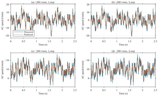
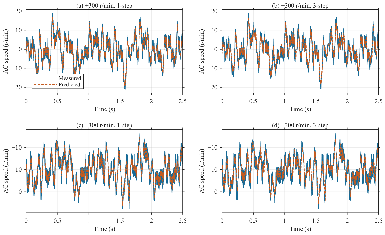
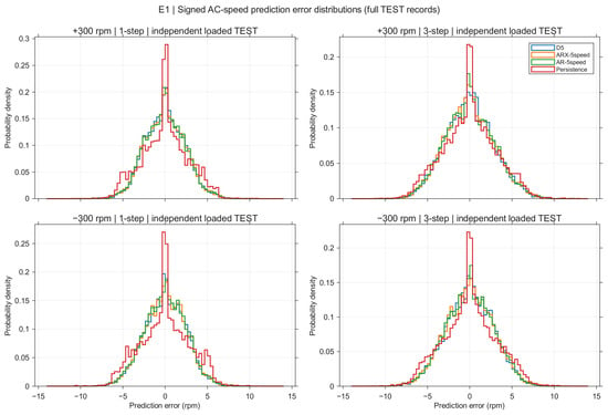
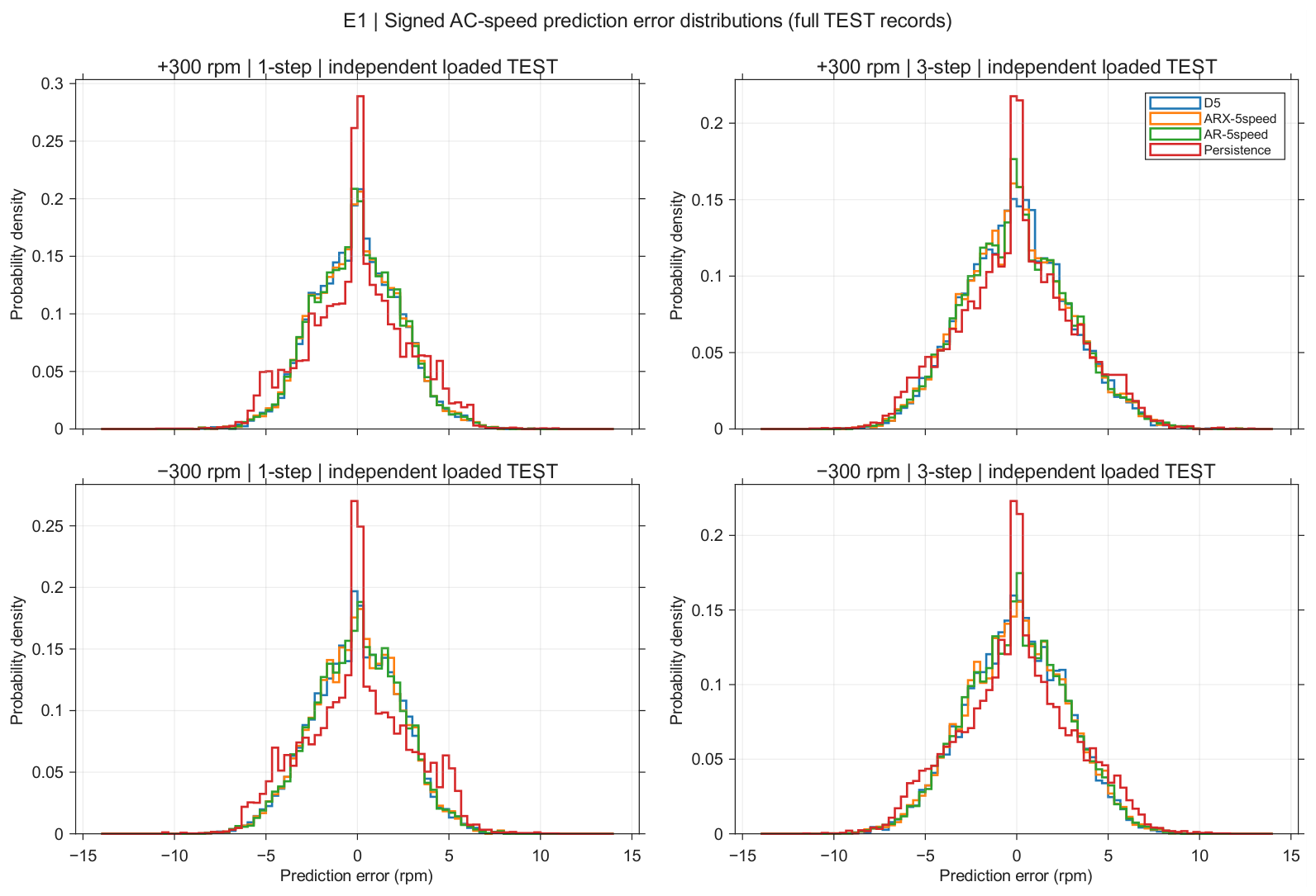
Table 3 reports the full-record prediction metrics, and Figure 4 shows the first 2.5 s of each record. At the three-step horizon used for control design, VAF reaches 83.955% for positive rotation and 78.045% for negative rotation. Compared with holding the current AC speed measurement constant over the same horizon, the models reduce RMSE by 8.08% and 10.90%, respectively. The learned dynamics improve prediction relative to persistence under the recorded input sequence. Section 5.5 compares the resulting feedback with proportional ripple damping.

Table 3. Held-out AC speed prediction of the structured D5 models. The final column gives the RMSE reduction relative to holding the current AC speed value over the same horizon.

Direction	Horizon	VAF (%)	RMSE (r/min)	Reduction vs. Hold (%)
Positive	1 step	89.378	2.3216	13.72
Positive	3 steps	83.955	2.8536	8.08
Negative	1 step	83.409	2.3958	16.07
Negative	3 steps	78.045	2.7563	10.90

Figure 4. Measured and predicted AC speed on the positive and negative direction held-out records. Each trace shows the first 2.5 s; Table 3 uses the full records.

Reconstructing the matched ARX realization described in Section 3.2 reproduces the archived matrices and predictions to floating-point precision (Table 4).

Table 4. AC speed prediction on independent loaded records. All models except persistence have five states. Matched ARX is equivalent to D5; speed-only models use different regressors and separately tuned regularization.

Direction	Predictor	VAF1 (%)	VAF3 (%)	RMSE3 (r/min)
$+300$	D5	89.378	83.955	2.8536
	Matched ARX	89.378	83.955	2.8536
	Speed history ARX	89.208	83.343	2.9075
	Speed history AR	89.184	83.243	2.9162
	Persistence	85.730	81.010	3.1045
$-300$	D5	83.409	78.045	2.7563
	Matched ARX	83.409	78.045	2.7563
	Speed history ARX	83.227	77.521	2.7889
	Speed history AR	83.170	77.341	2.8001
	Persistence	76.446	72.345	3.0934

The distinct five-state speed history ARX uses $[w_{\mathrm{ac},k},w_{\mathrm{ac},k-1},\dots ,w_{\mathrm{ac},k-4}]$ and the recorded auxiliary input; autoregressive (AR) modeling uses the same speed history without that input. Equal state dimension does not imply equal fitted parameter count: D5 estimates twelve dynamic coefficients per direction, whereas speed history ARX estimates six and AR five. Their regularization is selected on the unloaded training records. Supplementary Section S7 gives the tuning procedure.

The full-record three-step absolute error 95th percentiles are 5.608 r/min (positive) and 5.362 r/min (negative); Figure 5 shows the signed error distributions. Four consecutive portions of each test record give positive direction D5 three-step RMSE of 2.789–2.925 r/min and negative direction RMSE of 2.736–2.767 r/min (Supplementary Section S7, Figure S3).

Figure 5. Full-record signed AC speed prediction error distributions at one and three steps. ARX-5speed uses five speed history states; AR-5speed omits auxiliary input. Matched-ARX errors coincide with D5 and are not drawn twice.

5.2. Natural Ripple at the Nominal Operating Point

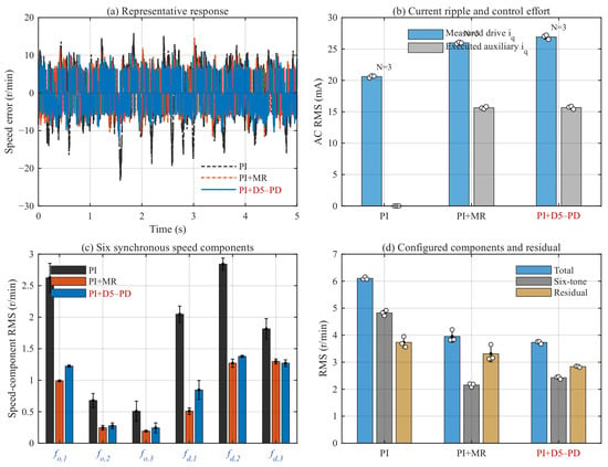
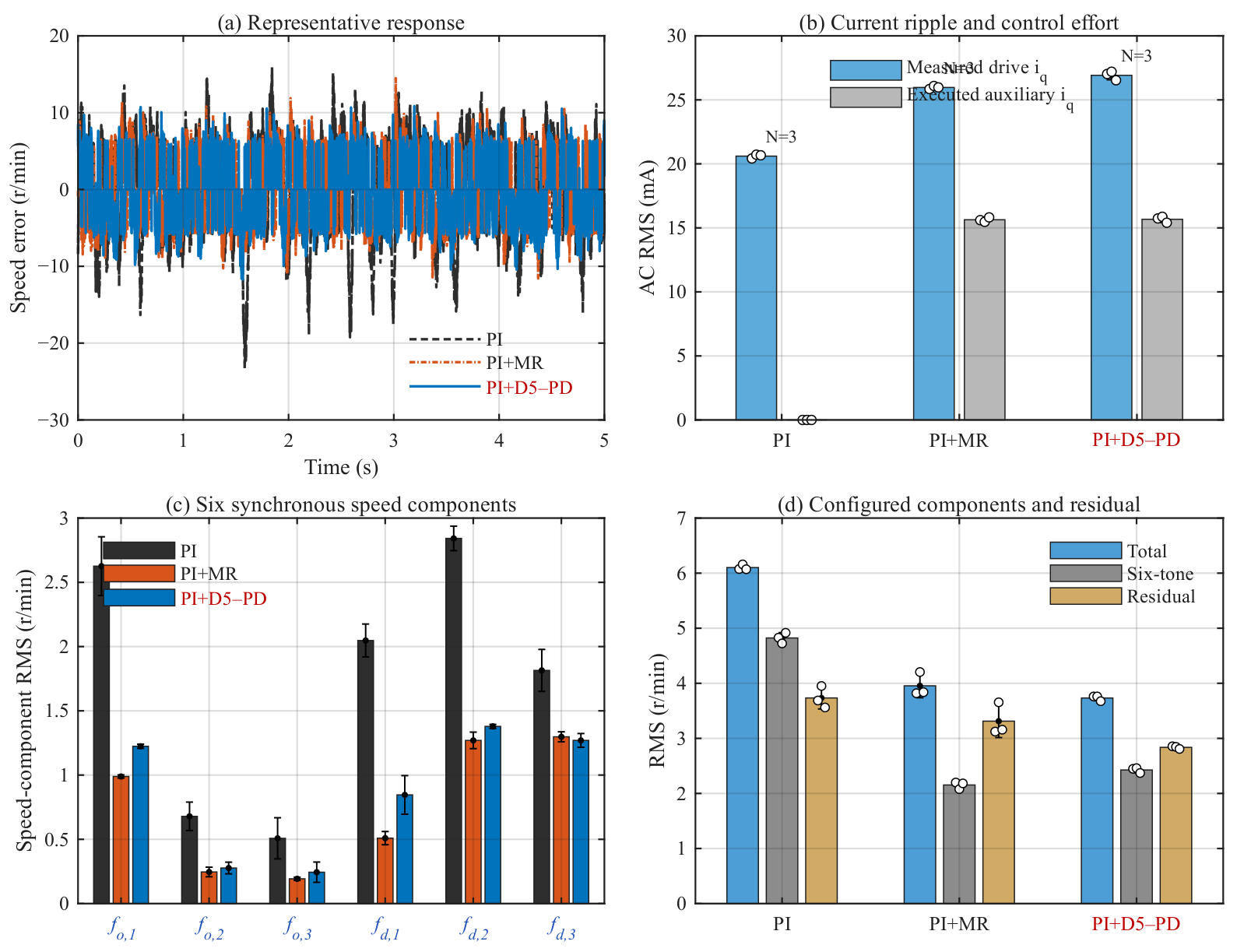
At the nominal operating point of $+300$ r/min and $+1$ A, D5–PD reduces mean speed ripple RMS by 38.83% relative to PI and 5.61% relative to MR (Table 5). This improvement is obtained at nearly equal auxiliary command AC RMS: $15.673\pm 0.240$ mA for D5–PD and $15.635\pm 0.177$ mA for MR.

Table 5. Repeated performance results (mean ± sample SD, $N=3$). RMS denotes total speed ripple RMS; $G_f$ denotes the load current-normalized response at the imposed frequency. Speeds in the condition labels are in r/min.

Condition	Metric	PI	PI + MR	PI + D5–PD
Natural +300/+1 A	RMS (r/min)	$6.1021\pm 0.0496$	$3.9547\pm 0.2172$	$3.7327\pm 0.0495$
2 Hz disturbance	$G_f$ (r/min/A)	$122.188\pm 13.275$	$75.124\pm 8.568$	$47.033\pm 6.743$
2 Hz disturbance	RMS (r/min)	$7.0990\pm 0.3422$	$4.4246\pm 0.2307$	$3.8857\pm 0.0606$
8 Hz disturbance	$G_f$ (r/min/A)	$92.391\pm 7.241$	$106.076\pm 4.268$	$42.251\pm 0.558$
8 Hz disturbance	RMS (r/min)	$6.8137\pm 0.4704$	$4.4618\pm 0.0556$	$3.8955\pm 0.1639$
Natural −300/−1 A	RMS (r/min)	$5.5954\pm 0.0816$	$3.6783\pm 0.0388$	$3.4575\pm 0.0851$
Natural +300/0 A	RMS (r/min)	$6.1012\pm 0.2420$	$4.0691\pm 0.2014$	$3.6513\pm 0.0822$
Natural +600/+1 A	RMS (r/min)	$5.5752\pm 0.0347$	$3.6671\pm 0.1034$	$3.8370\pm 0.0256$

The decomposition in Figure 6 clarifies the difference between the two auxiliary controllers. MR achieves the lower synchronous component metric, with $S_6=2.153\pm 0.065$ r/min compared with $2.426\pm 0.048$ r/min for D5–PD. After removal of these components, however, D5–PD achieves a residual RMS of $2.837\pm 0.025$ r/min, compared with $3.312\pm 0.298$ r/min for MR. Its residual RMS is therefore 14.36% lower, despite the higher $S_6$. Relative to PI, D5–PD reduces $S_6$ by 49.70% and $R_6$ by 24.02%, showing that its benefit extends to both synchronous and residual fluctuations. The lower total ripple obtained with D5–PD would not be apparent from a comparison of the six selected orders alone.

Figure 6. Natural-ripple results at $+300$ r/min and $+1$ A: (a) representative speed error waveforms; (b) measured drive current and executed auxiliary command AC RMS; (c) the six synchronous components, labeled $f_{o,1}$–$f_{o,3}$ and $f_{d,1}$–$f_{d,3}$ as defined in Equation (7); and (d) total, six-component, and residual RMS. Bars show means; error bars show sample SD; circles indicate individual runs where plotted. For each controller, the representative trace is the run whose speed AC RMS is closest to the median of its three repeated runs.

5.3. Response to 2 and 8 Hz Load Disturbances

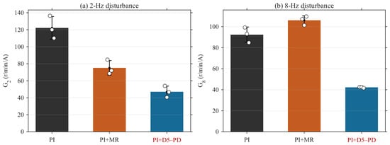
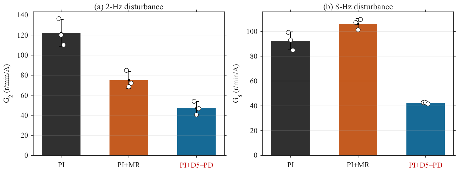
The 2 and 8 Hz disturbances test rejection at frequencies that do not coincide with the MR centers at 300 r/min. At 2 Hz, D5–PD reduces the mean load current-normalized speed response by 61.51% relative to PI and 37.39% relative to MR. At 8 Hz, the corresponding reductions are 54.27% and 60.17% (Table 5). Figure 7 shows the three individual runs for each controller.

Figure 7. Load current-normalized speed response at the two imposed disturbance frequencies. Bars show means, error bars show sample SD, and circles show individual runs ($N=3$).

At 8 Hz, MR produces a larger normalized response than PI, even though it attenuates the selected synchronous components more strongly. This result distinguishes rejection at an imposed frequency from suppression at the resonant centers. D5–PD also reduces total speed ripple RMS relative to MR by 12.18% in the 2 Hz test and 12.69% in the 8 Hz test. The same feedback gain and predictive weights are used as in the natural-ripple experiment, so these improvements require no retuning for either disturbance frequency.

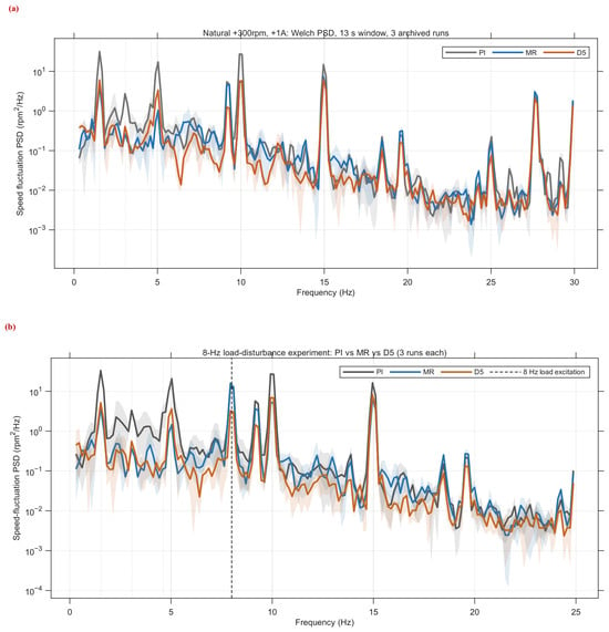
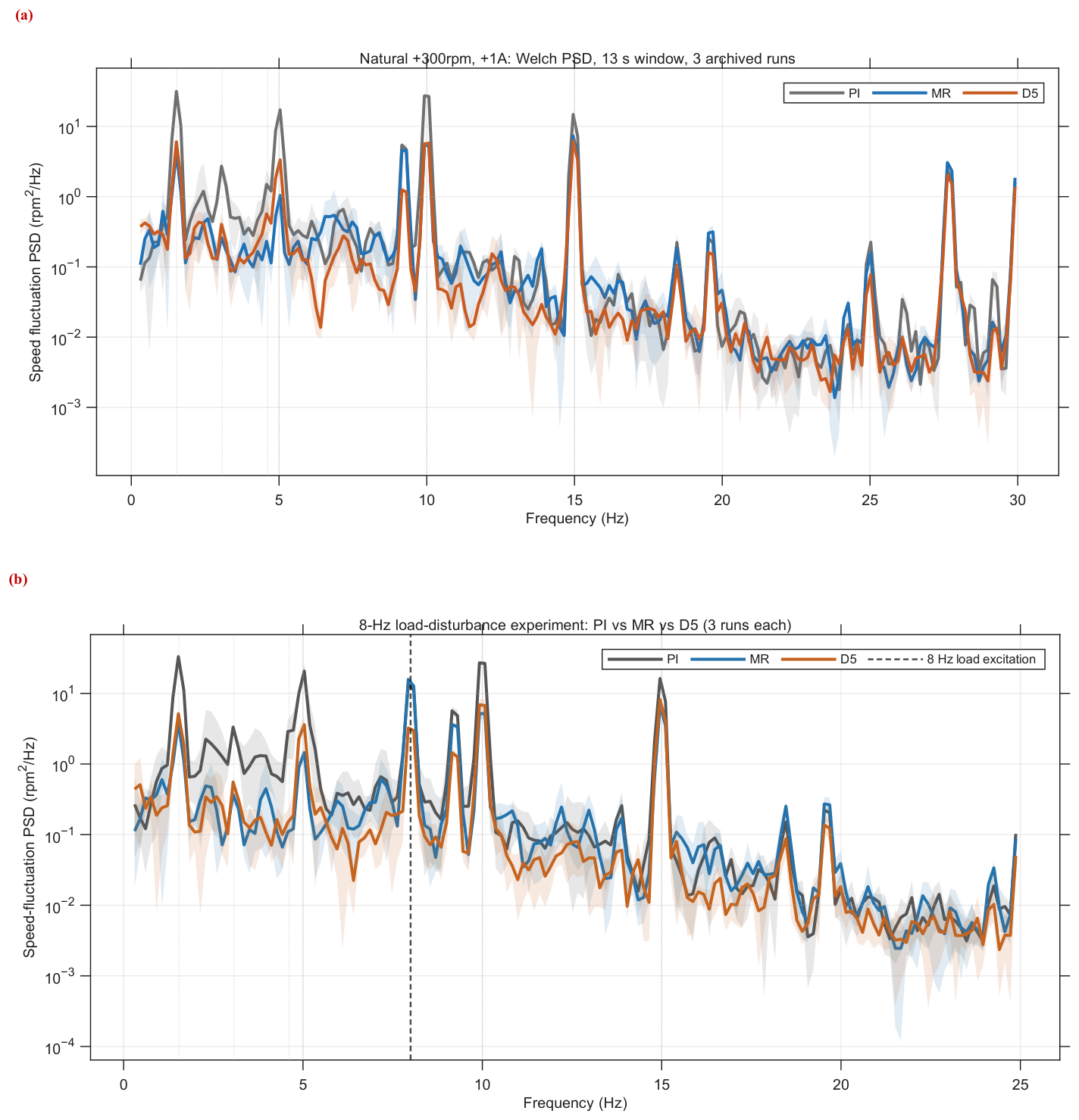
Figure 8 compares the measured speed spectra under natural ripple and the 8 Hz disturbance. In panel (a), MR more strongly attenuates the selected orders, whereas D5 gives lower residual RMS, consistent with Figure 6. In panel (b), MR has a larger 8 Hz component than PI despite lower total ripple. MR and D5 command AC RMS are $15.57\pm 0.48$ and $16.60\pm 0.77$ mA, respectively; their 8 Hz command components are approximately 2.13 and 4.30 mA. These observations distinguish selected-order attenuation from the response at the imposed frequency.

Figure 8. Measured drive speed Welch PSD at $+300$ r/min and $+1$ A: (a) natural ripple; (b) 8 Hz load disturbance. Each controller contributes three original 13 s windows, processed with identical PSD settings. Shading shows the three-run range. Vertical lines mark the six selected orders in (a) and the imposed 8 Hz frequency in (b). Both horizontal axes are frequency in hertz.

5.4. Reverse Rotation, Zero Load, and Operation at Higher Speed

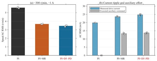
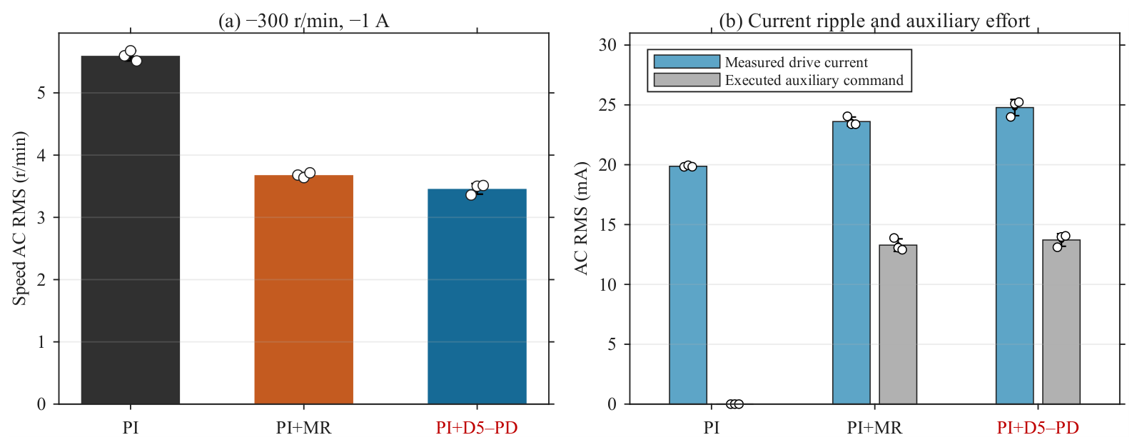
The reverse rotation test evaluates the controller with its negative direction feedback gain. At $-300$ r/min and $-1$ A, D5–PD reduces mean speed ripple RMS by 38.21% relative to PI and 6.00% relative to MR (Figure 9). At $+300$ r/min and zero load, the corresponding reductions are 40.15% and 10.27% (Table 5). The improvement over both benchmarks therefore extends beyond the nominal positive direction loaded condition.

Figure 9. Reverse-direction results at $-300$ r/min and $-1$ A: (a) speed AC RMS; (b) measured drive current and executed auxiliary command AC RMS. Means, sample SD, and the three individual runs are shown.

At $+600$ r/min and $+1$ A, D5–PD reduces mean total speed ripple RMS by 31.18% relative to PI, but gives 4.63% higher ripple than MR. MR shifts its resonant centers according to Equation (7), whereas D5–PD retains the positive 300 r/min gain and applies Equation (28). D5 has lower residual RMS (2.793 versus 2.995 r/min; Table 6) and lower auxiliary command AC RMS (10.94 versus 14.67 mA). These results document a tradeoff between total ripple, residual attenuation and command demand for the two implemented schedules; they do not isolate the effect of scheduling at equal effort. Additional speed-specific models and effort-matched repeated comparisons are therefore appropriate when extending operation beyond the identification point.

Table 6. Six synchronous components and residual ripple (mean ± sample SD, $N=3$). Frequencies are recalculated for each speed using Equation (7).

	Six Components ${\mathit{S}}_6$ (r/min)		Residual ${\mathit{R}}_6$ (r/min)
Condition	PI + MR	PI + D5–PD	PI + MR	PI + D5–PD
Natural +300/+1 A	$2.153\pm 0.065$	$2.426\pm 0.048$	$3.312\pm 0.298$	$2.837\pm 0.025$
2 Hz disturbance	$2.127\pm 0.104$	$2.438\pm 0.103$	$3.879\pm 0.219$	$3.025\pm 0.008$
8 Hz disturbance	$2.123\pm 0.081$	$2.501\pm 0.052$	$3.923\pm 0.101$	$2.986\pm 0.178$
Natural −300/−1 A	$1.864\pm 0.094$	$2.222\pm 0.125$	$3.170\pm 0.069$	$2.648\pm 0.007$
Natural +300/0 A	$1.906\pm 0.148$	$2.182\pm 0.077$	$3.590\pm 0.262$	$2.927\pm 0.049$
Natural +600/+1 A	$2.116\pm 0.030$	$2.629\pm 0.091$	$2.995\pm 0.111$	$2.793\pm 0.052$

5.5. Supplementary Repeatability and Linear Damping Benchmark at Reduced Load

The supplementary campaign uses $+300$ r/min and measured mean load-motor current 0.20 A, with no added 2/8 Hz disturbance. It contains six records each of PI, MR, D5 and SD. D5 uses the reported original gain, $\alpha =0.18$ configuration, and SD uses Equation (10). All records pass mode, speed, load and fixed-window quality control (QC).

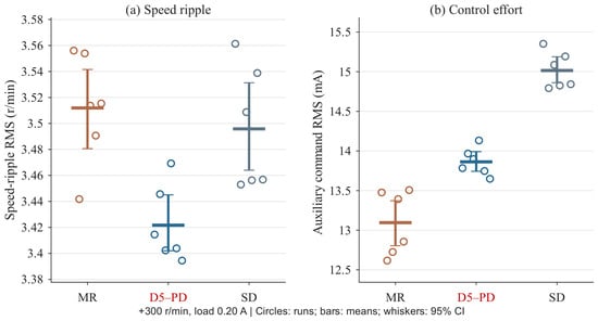
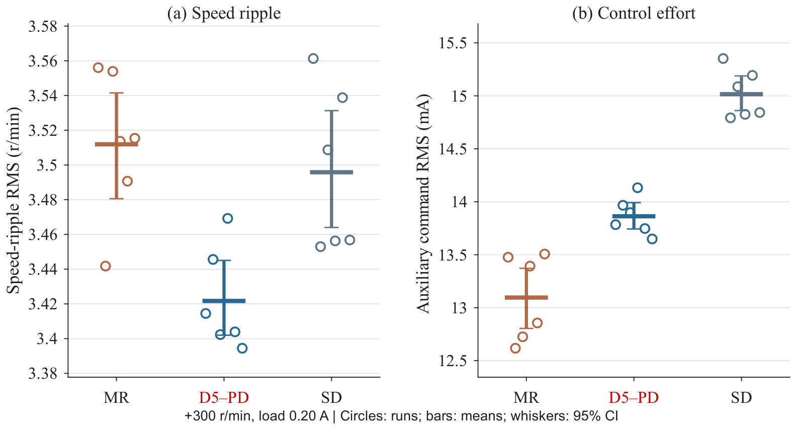
Each acquisition contributes one observation, using the settling interval and fixed window of Section 4.2 and the command RMS definition of Section 4.4. Figure 10 and Table 7 summarize the reduced-load comparison.

Figure 10. Reduced-load supplementary comparison. Circles show the six records of each auxiliary controller; bars show means; whiskers show unadjusted percentile bootstrap 95% confidence intervals for the means (20,000 independent group run resamples). PI results are given in Table 7; statistical definitions are in Supplementary Section S8.

Table 7. Supplementary benchmark at $+300$ r/min, 0.20 A. Values are mean ± sample SD over six records; $S_6,R_6$ columns show group means. Rate occupancy is the mean flagged sample percentage.

Method	N	Speed RMS (r/min)	Command RMS (mA)	${\mathit{S}}_6$ (r/min)	${\mathit{R}}_6$ (r/min)	Rate (%)
PI	6	$5.577\pm 0.126$	0	4.530	3.253	0
MR	6	$3.512\pm 0.043$	$13.096\pm 0.406$	1.644	3.103	0
D5	6	$3.422\pm 0.029$	$13.863\pm 0.173$	2.077	2.719	0
SD	6	$3.496\pm 0.047$	$15.015\pm 0.231$	2.212	2.706	1.597

SD reduces ripple relative to PI (Table 7). D5 gives mean speed ripple RMS of 3.422 r/min, 2.57% below MR and 2.12% below SD. Its residual RMS is lower than MR (2.719 versus 3.103 r/min), while SD has slightly lower residual RMS (2.706 r/min). MR gives the lowest six-order metric (1.644 versus 2.077 r/min for D5).

D5 command RMS is 5.86% above MR and 7.68% below SD. SD activates rate limiting for a mean 1.597% of samples; MR and D5 activate no rate flags. No amplitude or headroom flags occur in this supplementary benchmark.

Under the independent, exchangeable record assumption, exploratory two-sided permutation tests with Holm correction give $p=0.01299$ for D5 versus MR and $p=0.01515$ for D5 versus SD. Supplementary Section S8 reports the full contrasts, intervals and sampling assumptions.

5.6. Deployment-Scale Sensitivity at Reduced Load

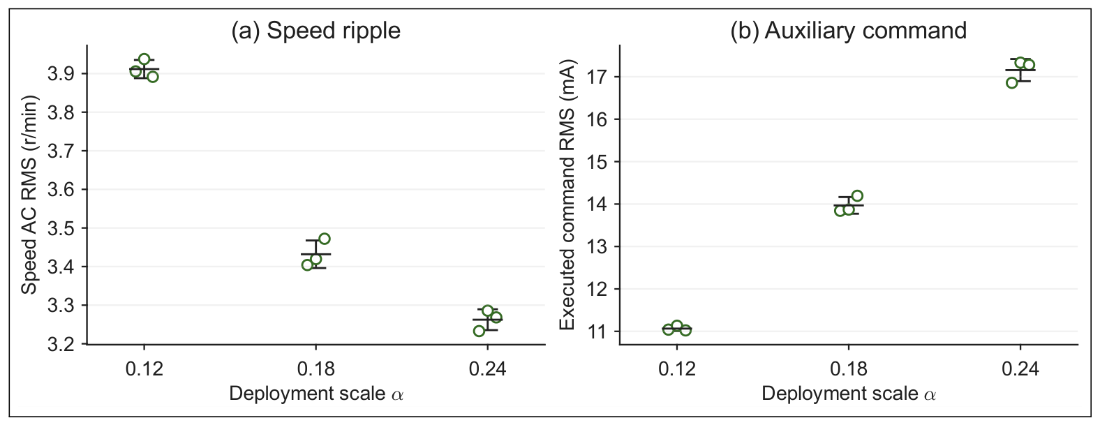
A separate sensitivity campaign evaluates $\alpha =0.12,0.18,0.24$ at $+300$ r/min and measured mean load 0.20 A, with three acquisition records per setting. The nine records are analyzed separately from the original 54-record campaign and the six-record-per-method benchmark, using the same 1 s settling interval and 13 s performance window. Scale groups follow the declared mode/state mapping, checked against CH6; record identities and provenance are given in Supplementary Section S9. Table 2 separately reports model-based weight sensitivity. Table 8 and Figure 11 summarize the measured deployment-scale tradeoff.

Table 8. Repeated deployment-scale sensitivity at $+300$ r/min and 0.20 A ($N=3$ per setting). Values are mean ± sample SD; $S_6,R_6$ are group means. Limiter columns give mean flagged-sample percentages.

$\mathit{\alpha }$	Speed RMS (r/min)	Command RMS (mA)	${\mathit{S}}_6$ (r/min)	${\mathit{R}}_6$ (r/min)	Amplitude (%)	Rate (%)
0.12	$3.912\pm 0.024$	$11.065\pm 0.059$	2.708	2.822	0	0
0.18	$3.432\pm 0.036$	$13.969\pm 0.196$	2.073	2.735	0	0
0.24	$3.262\pm 0.027$	$17.157\pm 0.261$	1.868	2.674	0.0513	0.0564

Figure 11. Repeated scale–ripple and scale–command-demand comparisons. Circles denote three acquisition records per setting; horizontal lines and whiskers denote mean ± sample SD. Record identities are listed in Supplementary Section S9.

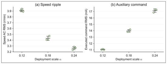
Relative to $0.18$, the $0.12$ setting gives 13.98% higher ripple and 20.79% lower command RMS; $0.24$ gives 4.94% lower ripple and 22.82% higher command RMS. At $0.24$, mean amplitude/rate occupancies are 0.0513%/0.0564%; neither limiter activates at $0.12$ or $0.18$. Stronger deployed feedback therefore improves ripple attenuation while increasing command demand and occasionally reaching the limits. The original $0.18$ setting is an intermediate operating point in this measured tradeoff.

5.7. Discussion of Synchronous and Residual Ripple Attenuation

Across the six conditions, D5–PD reduces mean residual RMS by 6.73–23.89% relative to MR (Table 6). MR consistently achieves the lower synchronous component metric $S_6$, but this advantage translates into lower total ripple only in the 600 r/min comparison. The distinction is central to the experimental findings: attenuation at selected orders and attenuation of the remaining waveform are separate aspects of speed control performance.

The results are consistent with the different control designs. MR places resonant action at specified synchronous frequencies, whereas D5–PD uses an identified dynamic relation between auxiliary current and measured speed history to penalize predicted speed fluctuations. Relative to PI, the latter reduces both synchronous and residual ripple at the nominal point; relative to MR, its clearest advantage is the lower residual fluctuation level and the improved response to the two imposed disturbances. This gives a practical basis for evaluating predictive damping alongside frequency-selective approaches [1,8], using total ripple and current demand in addition to individual harmonic components.

The reduced-load benchmark confirms that proportional ripple damping already reduces total ripple relative to PI. D5 gives a further 2.12% reduction with 7.68% less command RMS than SD, although SD has slightly lower residual RMS. This supports the implemented dynamic feedback at this operating point, while leaving the specific contribution of the three-step horizon unresolved. D4–D6 vary the delay-state dimension at a fixed horizon; isolating the horizon contribution requires a separate effort-matched comparison.

Implications for drive integration. The design addresses a retrofit task: the auxiliary model includes the action of the existing PI-regulated drive, and deployment uses a fixed feedback row with the same actuator interface as MR. The nominal comparison shows why total ripple and residual content matter alongside selected harmonics; the 2/8 Hz tests assess two off-center disturbances without adding resonant branches. The reduced-load SD result further connects ripple reduction to command demand. These findings support the engineering value of the complete implementation, while the matched-ARX result identifies its linear-model foundation.

6. Conclusions

This study demonstrates a compact auxiliary controller for speed ripple attenuation in a PI-regulated motor–reducer flexible drive. D5–PD combines direction-specific delay-coordinate models with exact history shifts and a three-step output-weighted design. Offline analytical synthesis yields fixed five-coefficient feedback, deployed at 1 ms intervals on an F28379D with current limits and the existing speed and inner current loops retained. The engineering contribution is the connection from measured drive speed history to experimentally evaluated embedded damping.

Across the six original conditions with three runs per controller, D5–PD gives lower mean total speed ripple RMS than PI in all conditions and than MR in five. At $+300$ r/min and $+1$ A, the reductions are 38.83% and 5.61%, respectively, with nearly equal auxiliary command AC RMS for D5–PD and MR. The load current-normalized responses at 2 and 8 Hz are 37.39% and 60.17% below MR without disturbance-specific retuning. MR gives stronger attenuation of the six selected synchronous components and lower total ripple at $+600$ r/min, whereas D5–PD gives lower residual RMS in all six conditions. The separate 0.20 A benchmark further shows 2.12% lower total ripple and 7.68% lower command RMS than proportional damping. Together, these results establish the measured tradeoff between total ripple, selected-order attenuation and command demand.

The sensitivity experiment shows that stronger deployment scaling can further reduce ripple at increased command demand and occasional limiting; it supports treating the original scale as a tested compromise rather than an optimum. The identified models remain local, and cross-speed deployment relies on empirical gain scaling rather than models identified at each speed. Further work should prioritize models at additional speeds and noise-aware identification, followed by effort-matched horizon comparisons and robustness analysis of the limited, scheduled loop.

References

- Zhang, Q.; Guo, H.; Liu, Y.; Guo, C.; Lu, K.; Wang, D.; Zhang, Z.; Sun, J. Robust plug-in repetitive control for speed smoothness of cascaded-PI PMSM drive. Mech. Syst. Signal Process. 2022, 163, 108090. [Google Scholar] [CrossRef] [Scilit]
- Yang, M.; Ni, Q.; Liu, X.; Xu, D. Vibration suppression and over-quadrant error mitigation methods for a ball-screw driven servo system with dual-position feedback. IEEE Access 2020, 8, 213758–213771. [Google Scholar] [CrossRef] [Scilit]
- Abouzeid, A.F.; Guerrero, J.M.; Vicente-Makazaga, I.; Muniategui-Aspiazu, I.; Endemano-Isasi, A.; Briz, F. Torsional vibration suppression in railway traction drives. IEEE Access 2022, 10, 32855–32869. [Google Scholar] [CrossRef] [Scilit]
- Chen, S.; Hu, M. Active torsional vibration suppression of hybrid electric vehicle drive system based on optimal harmonic current instruction calculation method. Mech. Syst. Signal Process. 2023, 205, 110837. [Google Scholar] [CrossRef] [Scilit]
- Szabat, K.; Orlowska-Kowalska, T. Vibration suppression in a two-mass drive system using PI speed controller and additional feedbacks—Comparative study. IEEE Trans. Ind. Electron. 2007, 54, 1193–1206. [Google Scholar] [CrossRef] [Scilit]
- Francis, B.A.; Wonham, W.M. The internal model principle of control theory. Automatica 1976, 12, 457–465. [Google Scholar] [CrossRef] [Scilit]
- Xia, C.; Ji, B.; Yan, Y. Smooth speed control for low-speed high-torque permanent-magnet synchronous motor using proportional–integral–resonant controller. IEEE Trans. Ind. Electron. 2015, 62, 2123–2134. [Google Scholar] [CrossRef] [Scilit]
- Zhang, Q.; Guo, H.; Guo, C.; Liu, Y.; Wang, D.; Lu, K.; Zhang, Z.; Zhuang, X.; Chen, D. An adaptive proportional-integral-resonant controller for speed ripple suppression of PMSM drive due to current measurement error. Int. J. Electr. Power Energy Syst. 2021, 129, 106866. [Google Scholar] [CrossRef] [Scilit]
- Wang, X.; Jiang, C.; Zhuang, F.; Lee, C.H.T.; Chan, C.C. A harmonic injection method equivalent to the resonant controller for speed ripple reduction of PMSM. IEEE Trans. Ind. Electron. 2022, 69, 9793–9803. [Google Scholar] [CrossRef] [Scilit]
- Guo, H.; Zhang, F.; Zhang, Q.; Liu, Y.; Xiang, T.; Xing, J. A Combined Fractional Order Repetitive Controller and Dynamic Gain Regulator for Speed Ripple Suppression in PMSM Drives. Actuators 2024, 13, 73. [Google Scholar] [CrossRef] [Scilit]
- Chai, S.; Wang, L.; Rogers, E. A Cascade MPC Control Structure for a PMSM With Speed Ripple Minimization. IEEE Trans. Ind. Electron. 2013, 60, 2978–2987. [Google Scholar] [CrossRef] [Scilit]
- Zhou, Z.; Xia, C.; Yan, Y.; Wang, Z.; Shi, T. Disturbances attenuation of permanent magnet synchronous motor drives using cascaded predictive-integral-resonant controllers. IEEE Trans. Power Electron. 2018, 33, 1514–1527. [Google Scholar] [CrossRef] [Scilit]
- Wang, C.; Yang, M.; Zheng, W.; Long, J.; Xu, D. Vibration suppression with shaft torque limitation using explicit MPC–PI switching control in elastic drive systems. IEEE Trans. Ind. Electron. 2015, 62, 6855–6867. [Google Scholar] [CrossRef] [Scilit]
- Sun, Z.; Hu, J.; Xin, Y.; Guo, Q.; Yao, Z.; Yang, Y. Active torsional vibration suppression for integrated electric drive system considering nonlinear factors. Nonlinear Dyn. 2024, 112, 17107–17127. [Google Scholar] [CrossRef] [Scilit]
- Gorla, A.; Serkies, P. Comparative Study of Analytical Model Predictive Control and State Feedback Control for Active Vibration Suppression of Two-Mass Drive. Actuators 2025, 14, 254. [Google Scholar] [CrossRef] [Scilit]
- Wróbel, K.; Śleszycki, K.K.; Majdański, P. Predictive Control Structure for a Two-Mass Drive System with a Two-Layer Observer. Energies 2025, 18, 6113. [Google Scholar] [CrossRef] [Scilit]
- Brunton, S.L.; Budišić, M.; Kaiser, E.; Kutz, J.N. Modern Koopman theory for dynamical systems. SIAM Rev. 2022, 64, 229–340. [Google Scholar] [CrossRef] [Scilit]
- Bevanda, P.; Sosnowski, S.; Hirche, S. Koopman operator dynamical models: Learning, analysis and control. Annu. Rev. Control 2021, 52, 197–212. [Google Scholar] [CrossRef] [Scilit]
- Strässer, R.; Worthmann, K.; Mezić, I.; Berberich, J.; Schaller, M.; Allgöwer, F. An overview of Koopman-based control: From error bounds to closed-loop guarantees. Annu. Rev. Control 2026, 61, 101035. [Google Scholar] [CrossRef] [Scilit]
- Williams, M.O.; Kevrekidis, I.G.; Rowley, C.W. A data-driven approximation of the Koopman operator: Extending dynamic mode decomposition. J. Nonlinear Sci. 2015, 25, 1307–1346. [Google Scholar] [CrossRef] [Scilit]
- Proctor, J.L.; Brunton, S.L.; Kutz, J.N. Dynamic mode decomposition with control. SIAM J. Appl. Dyn. Syst. 2016, 15, 142–161. [Google Scholar] [CrossRef] [Scilit]
- Proctor, J.L.; Brunton, S.L.; Kutz, J.N. Generalizing Koopman theory to allow for inputs and control. SIAM J. Appl. Dyn. Syst. 2018, 17, 909–930. [Google Scholar] [CrossRef] [Scilit] [PubMed]
- Korda, M.; Mezić, I. Linear predictors for nonlinear dynamical systems: Koopman operator meets model predictive control. Automatica 2018, 93, 149–160. [Google Scholar] [CrossRef] [Scilit]
- Arbabi, H.; Mezić, I. Ergodic theory, dynamic mode decomposition, and computation of spectral properties of the Koopman operator. SIAM J. Appl. Dyn. Syst. 2017, 16, 2096–2126. [Google Scholar] [CrossRef] [Scilit]
- Kamb, M.; Kaiser, E.; Brunton, S.L.; Kutz, J.N. Time-delay observables for Koopman: Theory and applications. SIAM J. Appl. Dyn. Syst. 2020, 19, 886–917. [Google Scholar] [CrossRef] [Scilit]
- Arbabi, H.; Korda, M.; Mezic, I. A Data-Driven Koopman Model Predictive Control Framework for Nonlinear Partial Differential Equations. In Proceedings of the 2018 IEEE Conference on Decision and Control (CDC); IEEE: Piscataway, NJ, USA, 2018; pp. 6409–6414. [Google Scholar] [CrossRef] [Scilit]
- Bruder, D.; Fu, X.; Gillespie, R.B.; Remy, C.D.; Vasudevan, R. Data-driven control of soft robots using Koopman operator theory. IEEE Trans. Robot. 2021, 37, 948–961. [Google Scholar] [CrossRef] [Scilit]
- Do, L.; Korda, M.; Hurák, Z. Controlled synchronization of coupled pendulums by Koopman model predictive control. Control Eng. Pract. 2023, 139, 105629. [Google Scholar] [CrossRef] [Scilit]
- Son, S.H.; Choi, H.K.; Moon, J.; Kwon, J.S.I. Hybrid Koopman model predictive control of nonlinear systems using multiple EDMD models: An application to a batch pulp digester with feed fluctuation. Control Eng. Pract. 2022, 118, 104956. [Google Scholar] [CrossRef] [Scilit]
- Zhang, X.; Pan, W.; Scattolini, R.; Yu, S.; Xu, X. Robust tube-based model predictive control with Koopman operators. Automatica 2022, 137, 110114. [Google Scholar] [CrossRef] [Scilit]
- Han, M.; Li, Z.; Yin, X.; Yin, X. Robust learning and control of time-delay nonlinear systems with deep recurrent Koopman operators. IEEE Trans. Ind. Inform. 2024, 20, 4675–4684. [Google Scholar] [CrossRef] [Scilit]
- Hanke, S.; Peitz, S.; Wallscheid, O.; Klus, S.; Böcker, J.; Dellnitz, M. Koopman Operator-Based Finite-Control-Set Model Predictive Control for Electrical Drives. arXiv 2019, arXiv:1804.00854v2. [Google Scholar] [CrossRef] [Scilit]
- Calderon, H.M.; Hammoud, I.; Oehlschlagel, T.; Werner, H.; Kennel, R. Data-Driven Model Predictive Current Control for Synchronous Machines: A Koopman Operator Approach. In Proceedings of the 2022 International Symposium on Power Electronics, Electrical Drives, Automation and Motion (SPEEDAM); IEEE: Piscataway, NJ, USA, 2022; pp. 942–947. [Google Scholar] [CrossRef] [Scilit]
- Kim, J.; Woo, H.; Choi, Y. Model Parameter-free Velocity Control of Permanent Magnet Synchronous Motor based on Koopman Operator. J. Korea Robot. Soc. 2022, 17, 308–313. [Google Scholar] [CrossRef] [Scilit]
- Wei, Y.; Chen, Y.; Zhang, Z.; Shuai, Z.; Young, H.; Wang, F. Model-Free Predictive Control Using Backward Koopman Operator-Based ARX on PMSM Drives. IEEE Trans. Ind. Electron. 2026, early access. [Google Scholar] [CrossRef] [Scilit]
- Carlet, P.G.; Favato, A.; Bolognani, S.; Dörfler, F. Data-Driven Continuous-Set Predictive Current Control for Synchronous Motor Drives. IEEE Trans. Power Electron. 2022, 37, 6637–6646. [Google Scholar] [CrossRef] [Scilit]
- Carlet, P.G.; Favato, A.; Torchio, R.; Toso, F.; Bolognani, S.; Dörfler, F. Real-Time Feasibility of Data-Driven Predictive Control for Synchronous Motor Drives. IEEE Trans. Power Electron. 2023, 38, 1672–1682. [Google Scholar] [CrossRef] [Scilit]
Disclaimer/Publisher’s Note: The statements, opinions and data contained in all publications are solely those of the individual author(s) and contributor(s) and not of MDPI and/or the editor(s). MDPI and/or the editor(s) disclaim responsibility for any injury to people or property resulting from any ideas, methods, instructions or products referred to in the content. |
© 2026 by the authors. Licensee MDPI, Basel, Switzerland. This article is an open access article distributed under the terms and conditions of the Creative Commons Attribution (CC BY) license.