A Robust Framework for Fault Diagnosis in Discrete Event Systems

Abstract

The reliability and safety of modern industrial applications demand efficient fault detection and isolation (FDI) systems. Unfortunately, traditional diagnostic techniques are often highly sensitive to measurement noise, leading to frequent false alarms. Additionally, many contemporary methods require exhaustive training datasets, limiting their practical applicability. To address these challenges, this paper proposes a novel hybrid diagnostic framework applied to a continuous fluid mixing and filling process. The presented framework combines continuous residual analysis with discrete-event temporal reasoning. A timed diagnoser, implemented using Stateflow, represents bounded time intervals as active behavioral guards to continuously monitor the system against nominal timelines. When a temporal violation is detected, a Fuzzy Inference System (FIS) is triggered to isolate the root cause. The FIS effectively resolves diagnostic ambiguities—particularly masking effects caused by concurrent actuator and sensor malfunctions by correlating continuous fluid levels with discrete temporal deviations. Extensive simulations under noisy conditions demonstrate that the proposed hybrid architecture achieves a 100% detection rate and a 99.0% fault localization accuracy, while completely eliminating false alarms (0% false alarm rate). These quantitative results significantly outperform classical observer-based techniques and standard discrete Petri net methodologies, confirming the robustness and superiority of the proposed framework.

1. Introduction

Data availability and fault diagnosis are essential elements of industrial control systems, which directly determine operational safety, productivity, and maintenance cost. Components like sensors and hydraulic actuators in complex fluid management systems—such as mixing and filling processes are constantly exposed to physical wear. A minor defect, such as an inaccurate sensor or a stuck valve, will propagate rapidly through the control loop and can result in process degradation or systemic failure. Therefore, it remains a significant challenge in control engineering to develop FDI systems that are both accurate and timely.

Historically, model-based diagnostic approaches [1], such as observer-based methods, have been extensively applied. Although these techniques are mathematically rigorous, they depend on constant residuals and thresholds, making them highly vulnerable to measurement noise and dynamic uncertainties, thus raising the false alarm rate. By contrast, standard Petri nets or classical state machines are purely discrete-event models with a particular ability to keep track of sequential logic, yet they very often fail in the stringent temporal-continuous coupling required for detecting subtle differences in chronometric timing. Recent data-driven approaches, especially neural networks, are promising; however, their applicability in practice is often limited due to the need for exhaustive, high-quality historical training datasets covering all potential fault scenarios.

To overcome these limitations, this paper introduces a hybrid diagnostic architecture that synergizes continuous physical dynamics, temporal reasoning, and fuzzy logic. The primary contributions of this work are threefold:

• Hybrid Dynamic Modeling: The formulation of a baseline operational model that accurately maps the discrete logic of the process to its continuous fluid dynamics.
• Timed Diagnoser Implementation: The development of a supervisory module integrating bounded time intervals as strict behavioral guards, enabling the instantaneous detection of temporal delays and operational anomalies.
• Fuzzy Fault Isolation: The design of a Fuzzy Inference System (FIS) capable of resolving complex diagnostic ambiguities [2]. By correlating physical state variations with temporal alarms, the algorithm accurately discriminates between concurrent actuator and sensor faults.

To provide a comprehensive theoretical context for anomaly management in Discrete Event Systems (DES), it is crucial to acknowledge the broader diagnostic and control paradigms beyond standard Fault Detection and Isolation (FDI). In recent years, significant research has focused on robust Fault-Tolerant Control (FTC) strategies, which aim to maintain system stability and performance thresholds despite active component degradation [3]. For instance, observer-based fault-tolerant predictive control schemes for linear parameter-varying (LPV) systems have been shown to estimate and compensate sensor faults online without requiring a dedicated fault isolation module [4]. For repetitive industrial operations such as sequential fluid mixing and batch filling cycles, Iterative Learning Control (ILC) architectures have been effectively deployed to dynamically reject persistent disturbances and improve transient tracking accuracy over successive iterations [5]. While these advanced methodologies offer robust frameworks for overall system control and scheduling, the hybrid approach proposed in this paper specifically targets the critical prerequisite of instantaneous fault isolation. By coupling timed automata with fuzzy logic inference, the proposed framework complements these broader DES control strategies by ensuring that temporal violations are accurately diagnosed before triggering an FTC reconfiguration.

The necessity for robust fault diagnosis and tolerance is a growing concern in modern complex continuous processes, particularly when continuous dynamics must be governed by discrete-event supervisory control [6]. Recent literature highlights the increasing reliance on fuzzy logic and robust control algorithms to manage system uncertainties, ensure disturbance rejection, and maintain strict operational safety. For instance, advanced fuzzy-based adaptive frameworks have been successfully developed to guarantee fault-tolerant performance in complex nonlinear systems operating under periodic event-triggered communication mechanisms [7]. Similarly, to guarantee strict temporal performance bounds and robust disturbance rejection against external anomalies, predefined-time sliding-mode control strategies have recently proven highly effective [8,9].

The proposed framework is empirically validated through the simulation of targeted fault injections (e.g., varying degradation severities in valves and level sensors). The results highlight the complete elimination of false alarms (0% rate) and a near-perfect localization accuracy (99.0%), significantly outperforming classical diagnostic methods.

While existing literature has explored the intersection of timed automata and fuzzy logic for diagnostic purposes, most conventional approaches focus on fuzzifying the temporal transitions themselves. This strategy inherently softens the behavioral constraints, which can compromise the deterministic safety and real-time guarantees required in critical industrial processes.

The specific novelty of the proposed hybrid framework lies in its decoupled, two-stage architecture, which efficiently bridges Discrete Event Systems (DES) and continuous dynamics without the computational explosion typical of full hybrid automata. The methodological improvements are twofold: First, a deterministic Timed Automaton is employed exclusively for real-time fault detection, leveraging rigid, mathematically defined temporal guards to immediately flag chronometric deviations. Second, upon detection, a targeted Fuzzy Inference System (FIS) is activated specifically for fault isolation. The FIS introduces a significant improvement over standard discrete diagnosers by cross-referencing the discrete temporal alarm delay with the continuous physical residual (fluid mass-balance). This unique integration effectively resolves the isolation ambiguity between functionally coupled actuator and sensor faults, a known limitation in purely discrete diagnostic models, ensuring high precision and reliability in complex sequential manufacturing operations.

The remainder of this paper is organized as follows: Section 2 details the physical description of the industrial fluid process. Section 3 develops the timed diagnoser and the fuzzy isolation principle. Section 4 applies the framework to the mixing process, including the identification of the temporal parameters and the tuning of the fuzzy isolation module. Section 5 presents the simulation results and the dynamic validation of the fault injection scenarios. Section 6 provides a quantitative comparative analysis against observer-based and Petri net methodologies. Finally, Section 7 concludes the study and discusses future research directions.

2. Process Description and Physical Modeling

2.1. Continuous Dynamics and Plant Model

The physical system is a chemical mixing process consisting of a main tank fed by two raw material silos (Ingredients 1 and 2). To align the continuous plant dynamics with the linear clock constraints of the diagnostic Timed Automata, the drainage process is modeled as an active constant-rate extraction (Q_S = 0.307 m³/s) rather than a gravity-driven Torricelli flow.

Consequently, the variations in the liquid volume V(t) and the fluid height h(t) inside the tank are governed by the following linear mass-balance equation:

$$S\cdot {\displaystyle \frac{\mathit{dh}\left(t\right)}{\mathit{dt}}}=Q_A\cdot V_A\left(t\right)+Q_B\cdot V_B\left(t\right)-Q_S\cdot V_S\left(t\right)$$

(1)

where S is the tank cross-sectional area, and V_A(t), V_B(t), and V_S(t) represent the discrete Boolean commands {0,1} applied to the respective valves.

To ensure the full reproducibility of the simulations presented in this paper, the nominal physical parameters and initial conditions of the process are detailed in Table 1.

Table 1. Physical Parameters of the Mixing Process.

Physical Parameter	Symbol	Nominal Value
Maximum tank height	Hmax	5.0 m
Tank cross-sectional area	S	1.0 m2
Maximum volumetric capacity	Vmax	5.0 m3
Ingredient 1 flow rate	QA	0.222 m3/s
Ingredient 2 flow rate	QB	0.222 m3/s
Drainage flow rate	Qs	0.307 m3/s

Initial Conditions at t = 0: h(0) = 0 m, C(0) = 0 kg/m³, and all valves are closed (VA = VB = VS = 0).

2.2. Product Concentration and Uncertainty Propagation

To guarantee product quality, the final concentration C (in kg/m³) must strictly remain within the acceptable interval C ∈ [C_min, C_max]. This concentration depends entirely on the introduced masses m₁, m₂, given that the initial concentrations C₁ and C₂ of the two raw ingredients are inherently uncertain:

$$C=f\left(C_1,C_2\right)={\displaystyle \frac{m_1+m_2}{\frac{m_1}{C_1}+\frac{m_2}{C_2}}}$$

(2)

To evaluate the impact of these uncertainties, a first-order Taylor series expansion (linearization) is applied around the nominal operating point (C₁₀, C₂₀):

$$\Delta C\approx {\left({\displaystyle \frac{\partial f}{\partial C_1}}\right)}_0\Delta C_1+{\left({\displaystyle \frac{\partial f}{\partial C_2}}\right)}_0\Delta C_2$$

(3)

Assuming the parameter variations follow a normal distribution, the overall standard deviation of the final concentration σ_C is derived through the variance propagation formula:

$${\sigma }_C=\sqrt{{\left({\displaystyle \frac{\partial C}{\partial C_1}}\right)}^2{\sigma }_{C_1}^2+{\left({\displaystyle \frac{\partial C}{\partial C_2}}\right)}^2{\sigma }_{C_2}^2}$$

(4)

For the simulated production batch, the target operating conditions rely strictly on the introduction of the two raw ingredients. Applying this statistical model establishes the critical tolerance interval for the final concentration based on the added masses m₁ and m₂. Any deviation exceeding this threshold compromises the mixture quality and must be promptly isolated by the diagnoser. For this specific simulation cycle, the target masses are mapped directly to the discrete fluid heights monitored by level sensors L2 (2.0 m) and L3 (4.0 m), given the 1 m² tank cross-section.

2.3. Fuzzy Residuals and Timed Diagnoser

The continuous fluid level h(t) is abstracted into discrete events via level sensors (L₁, L₂, L₃), whose activation timings are monitored. Fault detection relies on generating continuous residuals r(t), evaluated by a Fuzzy Inference System (FIS). The fuzzy aggregation generates a global confidence index γ(t).

This index is coupled with a Timed Automaton to filter false alarms and isolate specific faults. The event-driven and temporal dynamics of the supervisor are formally modeled by a Fuzzy Interval Petri Net (FIPN), defined as:

FIPN = ⟨P, T, Pre, Post, M₀, τ, μ⟩

(5)

The evolution of the system’s discrete state is governed by the standard Petri net state equation:

M_k+1 = M_k + W ⋅ U_k

(6)

where M_k is the marking vector (e.g., active state S₁), W = (Post − Pre) is the incidence matrix, and U_k is the firing vector (sensor inputs such as L₁ or L₂).

As illustrated in our simulation results, the isolation of Fault D₀ (specifically corresponding to the delayed activation of sensor L₂) is mathematically triggered if the maximum allowed time constraint τ_max(L₂) expires while the fuzzy validation remains active:

M_k+1(p_D0) = 1 ⟺ (Clock > τ_max(L₂)) ∧ (γ(t) ≥ γ_th)∧(M_k(p_S1) = 1)

(7)

Upon triggering this transition, the diagnoser marking updates to the fault state D₀, activating the isolation alarm and immediately enforcing safe shutdown commands (e.g., switching VA to OFF), as successfully demonstrated in the actuator command simulations.

3. Development of the Diagnoser

A diagnoser functions as an active supervisor, monitoring the execution of processes and raising alarms once it detects certain anomalies. Since internal faults are not directly observable, the system must infer their existence by analyzing logged events and their time intervals. One can build a framework from timed automata, which involves defining precise tracking problems associated with the temporal development of the system being modeled. Sampath et al. originally developed the basic principle of discrete event systems diagnosis [6], which generated great interest and research on deterministic timed automata for this task.

The commonality of these strategies is the underlying need for a detailed model that encompasses the entire spectrum of operational scenarios from nominal to degraded and an exhaustive behavioral map of the monitored process [10].

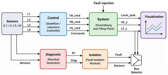
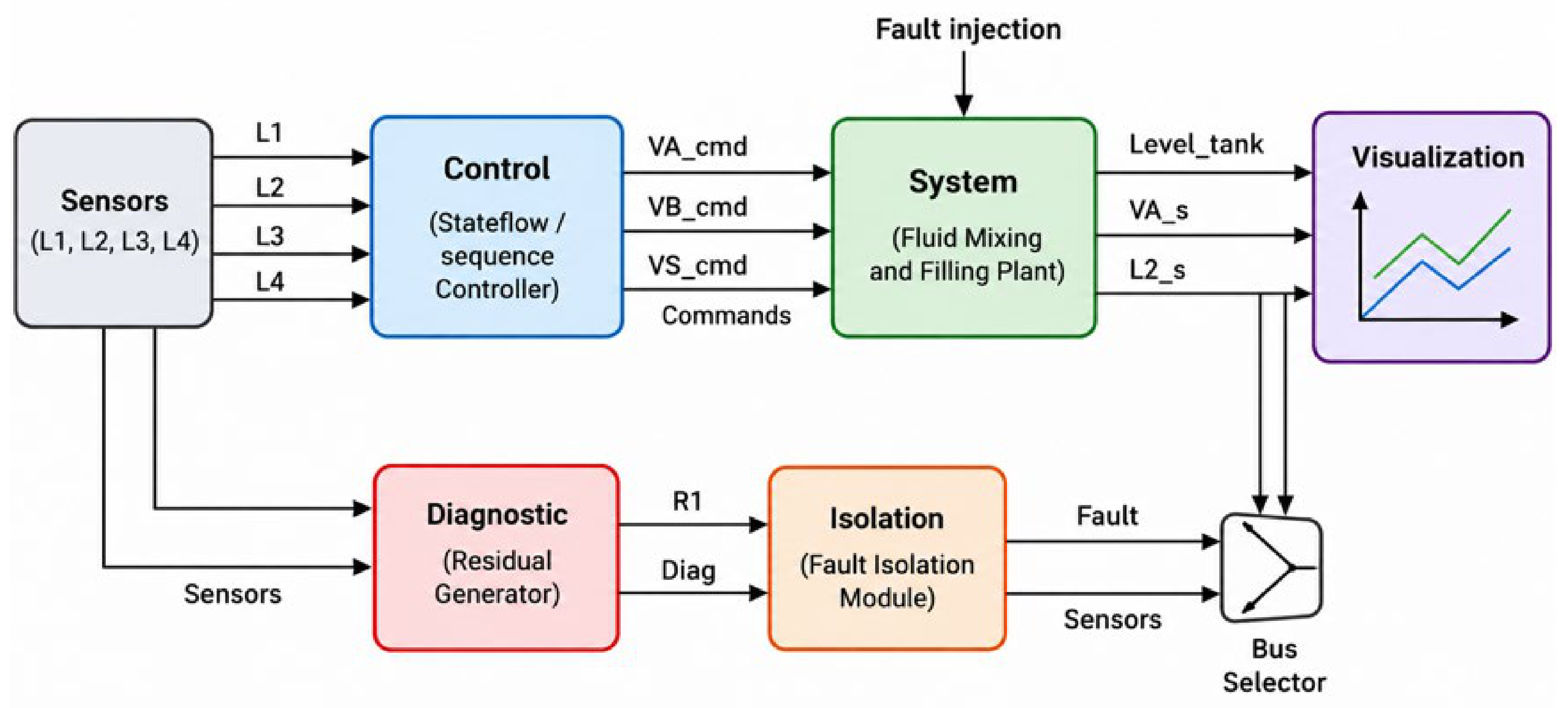
In this work, we develop the proposed diagnoser over two different but complementary models one for normal, healthy operations and another characterizing abnormal conditions. The total design architecture of this dual-model framework is depicted in Figure 1.

Figure 1. Global architecture of the proposed fault diagnosis and isolation (FDI) framework.

As illustrated, the overall system is composed of several key interactive modules:

• Control Module: A Stateflow/sequence controller that processes sensor data (L1 to L4) to generate nominal command signals (VA_cmd, VB_cmd, VS_cmd).
• System Plant: The physical fluid mixing and filling process, which is subjected to external fault injections.
• By producing discrete diagnostic signals (Diag) and continuous residuals (R1) based on real-time sensor discrepancies, the Diagnostic Module (Fault Detection) serves as the reference model.
• Isolation Module (Fault Location): Processes the generated residuals to explicitly isolate the root cause and output the definitive fault status.

3.1. Applications of Timed Automata in System Monitoring

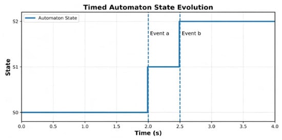
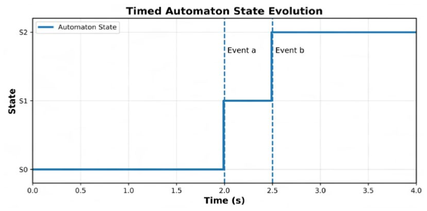
In 1990, Alur and Dill introduced Timed Automata [11], which are currently widely utilized to represent Real-Time Systems. By including continuous variables (referred to as clocks), this model expands upon classical finite state machines, which progress continuously over time. Transitions within a system are controlled by certain temporal constraints (guards) and may reset the clock. In addition, each state has invariants, which are temporal conditions that should remain true as long as the system is in this state (there must always be at least one). This architecture allows enforcing hard timing rules (for example, the minimum delay between two consecutive transitions) or blocking a transition if a temporal deadline expires, making it exceptionally well-suited for capturing real-time dynamics [11]. This path of research remained alive after the development of algorithms for model-checking timed automata. Once some theoretical foundations were laid down, practical applications began to materialize: modeling temperature fluctuations in controlled environments or designing event recorders for industrial controllers. In summary, timed automata provide a rich modeling framework for specifying and monitoring real-time dynamic systems [12]. Timed automata allow systems to be represented in both qualitative and quantitative dimensions, as depicted in Figure 2. Qualitative Variables describe the event ordering (such as a and b), while Quantitative Variables express temporal events (x₁, x₂).

Figure 2. State evolution of the timed automaton during normal operation.

While the automaton is in state S_i, its clock x_i is continuously increasing, so the model contains exact timing information. This evolution is represented in Figure 2 by the relation $\dot{ x}=1$. For instance, we have two clocks at x₁, and x₂. Every state has an invariant that specifies how long the system can remain in that state. Therefore, the guard for the output transition from state S₀ is defined by the condition a ∧ (x₂ = 2).

Figure 2 attests to dynamic behavioral tracking of the timed automaton. The system starts in its nominal state S₀. At t = 2.0 s, Event ‘a’ satisfies the temporal guard condition of the clock, which is perfectly aligned with the temporal guard, hence a discrete transition to state S₁ under the firing of Event ‘a’ takes place and the clock resets. Then at t = 2.5 s, the occurrence of Event ‘b’ in the allowed temporal interval satisfies the invariant and the system is moved to state S₂. This simulation also serves to validate the integer clock automaton, which imposes with precision qualitative event sequencing and quantitative timing constraints, an important requirement if the temporal abnormality is to be singled out in the diagnostic phase.

3.2. Hybrid Structure of Timed Automata Coupled with Fuzzy Diagnosis

In this section, we introduce the hybrid model that combines TA with Fuzzy Diagnosis. The goal is to give a formal description of the integration of temporal reasoning and uncertainty handling in fault diagnosis.

• Timed Automata Modeling

A timed automaton is defined as a tuple A = (Q, Σ, C, E, q₀, Inv), where Q is a finite set of discrete states, Σ is the finite alphabet of observations, C is a finite set of clocks, E ⊆ Q × Σ × B(C) × 2^C × Q is a finite set of transitions, q₀ ∈ Q is the initial state, and Inv: Q → B(C) gives each state an invariant condition over the clocks.

If the guard g over the clocks is satisfied, each transition e = (q_i, σ, g, R, q_j) is enabled. The clocks in R are reset when the transition is triggered.

• Continuous Residual Generation

The system’s continuous-time dynamics are provided by:

$$\dot{\mathrm{x}}\left(\mathrm{t}\right)=\mathrm{f}\left(\mathrm{x}\left(\mathrm{t}\right),\mathrm{u}\left(\mathrm{t}\right),\mathsf{\theta }\right)$$

(8)

Y(t) = h(x(t))

(9)

Residuals are generated as [13,14]:

r_i(t) = y_i(t) − ŷ_i(t)

(10)

• Fuzzy Evaluation of Residuals

Each residual is evaluated using fuzzy membership functions representing different fault levels:

$${\mu }_{r_i}^k\left(t\right)={\mu }^k\left(r_i\left(t\right)\right), k\in \{\mathrm{Healthy}, \mathrm{Actuator} \mathrm{Fault}, \mathrm{Sensor} \mathrm{Fault}\}$$

(11)

r_i(t) Represents the continuous physical residual generated at time t, and μ^k denotes its calculated degree of membership to a specific fuzzy linguistic set k ∈ {Healthy, Actuator Fault, Sensor Fault}.

A fuzzy inference system aggregates the residual information to compute a fault confidence index:

$$\gamma \left(t\right)=F\left({\mu }_{r_1}\left(t\right),{\mu }_{r_2}\left(t\right),\dots ,{\mu }_{r_m}\left(t\right)\right)$$

(12)

F denotes the fuzzy aggregation operator (e.g., standard Mamdani inference) that processes the individual residual memberships to compute γ(t), which serves as the overall global fault confidence index for the system.

• Coupling Between Timed Automata and Fuzzy Diagnosis

The coupling is achieved by linking fuzzy fault confidence levels to the transition guards of the timed automaton [2,11,12].

γ(t) ≥ γ_th and τ_f ≤ c_f ≤ T_f

(13)

γ_th: The predefined critical threshold for the fuzzy confidence index. A diagnostic transition is only considered if the aggregated fuzzy belief γ(t) exceeds this value.

c_f: The active continuous local clock of the timed automaton.

τ_f: The lower temporal boundary. In the context of the transition guard, it acts as a temporal persistence filter.

T_f: The upper temporal boundary, which corresponds to the maximum permissible physical deadline for the operation (e.g., the nominal filling time limit).

Consequently, the temporal decision condition ensures that a definitive fault state is only triggered if the physical severity of the residual is sufficiently high (γ(t) ≥ γ_th) AND the temporal progression of the event is strictly validated within the critical evaluation window (τ_f ≤ c_f ≤ T_f).

• Hybrid Diagnosis Decision Law

The hybrid diagnosis decision law is therefore defined as follows, where a fault f is confirmed only when the timed automaton reaches the corresponding fault state:

$$\mathrm{Diagnosis}\left(t\right)=\left\{\begin{array}{cc}\mathrm{Healthy}& \mathrm{if}\gamma \left(t\right)<{\gamma }_{\mathit{th}}\\ \mathrm{Fault}f& \mathrm{if}\gamma \left(t\right)\ge {\gamma }_{\mathit{th}}\end{array}\right.$$

(14)

3.3. Detection Principle

The dynamic model of the system is constructed as a network of timed automata. As a control and monitoring instrument, it collects temporal data (such as duration of operations, sequencing of tasks, and timing of event occurrences).

This holistic time domain view of the process allows for recognition and sensing of process errors using granular behaviors of expected and observed actions.

It can always know exactly what to anticipate thanks to its local view of the observed process. Every time a discrepancy occurs, whether it be in the measurement’s value or the event’s timing, it is promptly identified as a fault, making abnormalities easier to spot.

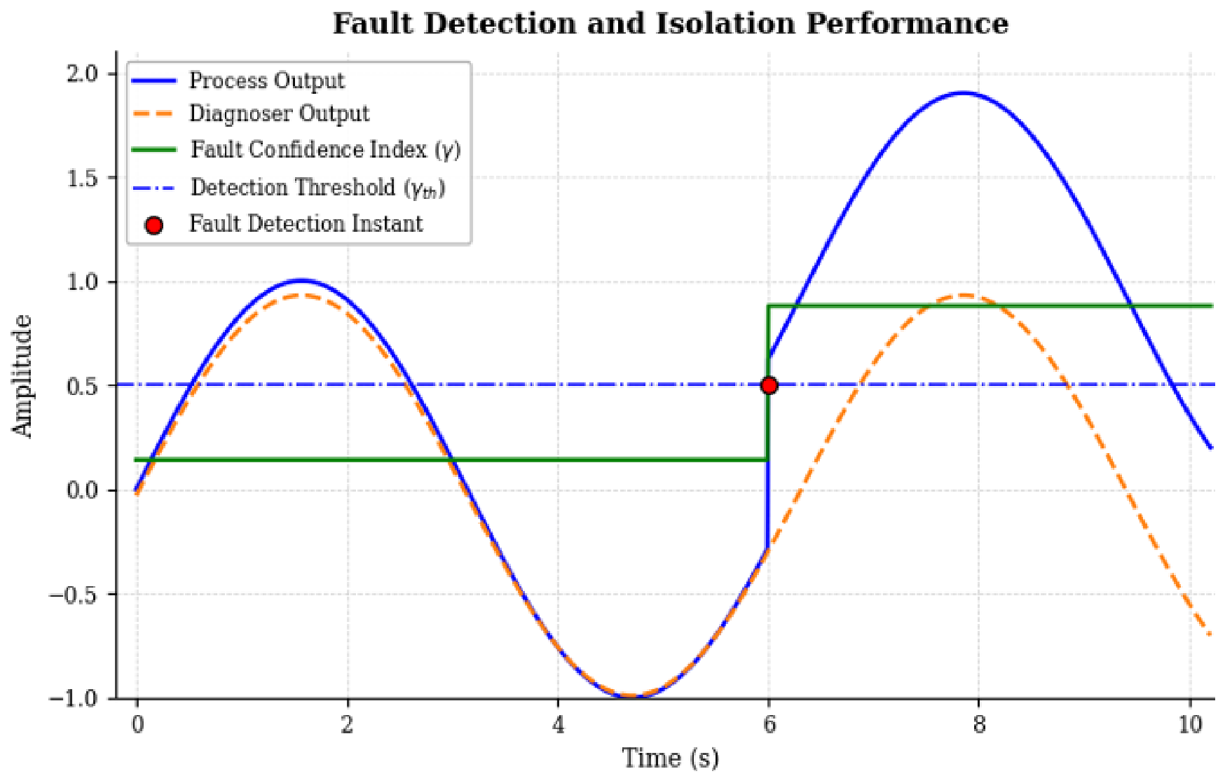
Figure 3 shows the real-time performance of the hybrid diagnostic decision law. The real process output (solid blue line) and the estimated diagnoser output (dashed orange line) from t = 0 to t = 6.0 s demonstrate the healthy operation phase. During that time, the residual is small [10], keeping the fuzzy fault confidence index (γ) far below the a priori detection threshold (γ_th). At t = 6.0 s, a fault is introduced, which produces an instantaneous divergence between the anticipated dynamic model behavior and the real system response. As a result, the residual rises and the fuzzy confidence index experiences a sudden jump. When γ passes the set threshold value (γ_th), the diagnostic logic confirms the inconsistency and an alarm is immediately raised (indicated by the red marker). This confirms the framework’s ability to be highly sensitive to abrupt faults while successfully signaling anomalies in an online fashion without generating false positives under nominal conditions.

Figure 3. Dynamic response of the fault detection framework comparing process and diagnoser outputs.

3.4. Faults Location

For fault localization, a fuzzy rule-based technique is proposed. This method deals with residuals produced by the detection module while considering aspects of uncertainty in the measurements of physical systems [15]. Unlike traditional control loops, which can have difficulty handling qualitative or vague information, fuzzy logic resembles human thinking processes. It allows for consistent decisions even in the presence of incomplete and fuzzy input data, thus promising an overall more reliable diagnostic scheme.

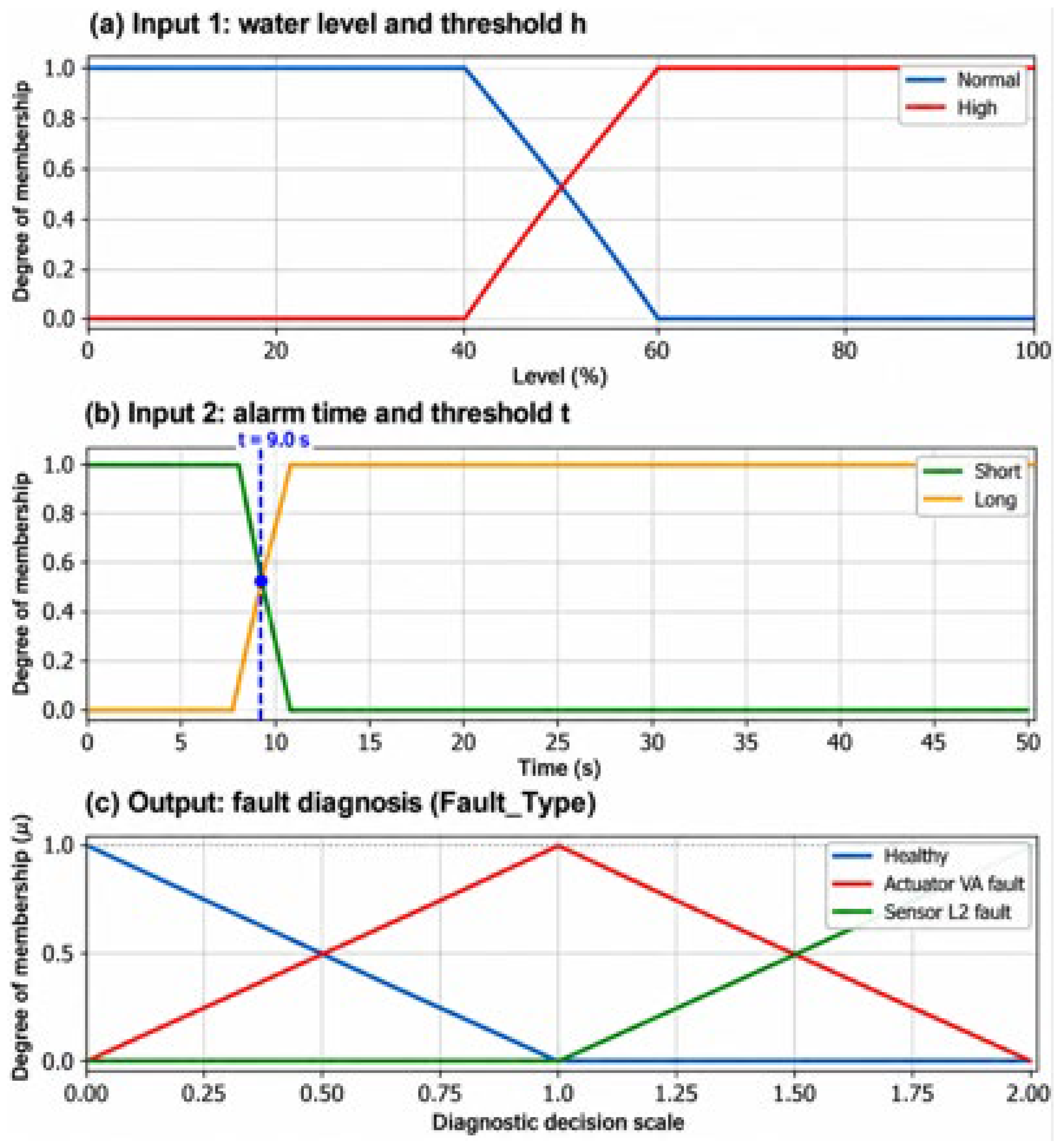
A fuzzy set expresses the degree of gradual membership of an element to a set, with its elements having a membership grade ranging between 0 and 1. A number of membership functions, including triangular, trapezoidal, and Gaussian, are used to represent these relations [16]. The fuzzy controller is based on a number of IF-THEN rules of the form IF condition THEN action, which are usually derived from experience-based process knowledge. As shown in Figure 4, the processing of this controller can be summed up into three main stages: the fuzzification of numerical inputs, the fuzzy execution on the rule base, and the defuzzification of actionable numerical outputs.

Figure 4. Architecture and functional response of the proposed fuzzy logic diagnostic controller.

Within this scheme, fuzzy logic observes threshold violations to monitor component degradation. Real sensor and actuator readings are constantly being compared to what they should be under the current operational regime. Differences are processed according to a set of fuzzy rules predefined to help isolate and identify the faulty module. The system, designed in the MATLAB/Simulink environment, utilizes two input parameters: the physical water level and the elapsed alarm time, matching them to isolate timing errors and identify specific faults [14].

The fuzzy inference system is realized in three stages as shown in Figure 4. The fuzzification process in the upper plots (a and b) discretizes two physical input variables: the water level into “Normal” and “High”, and the alarm time into “Short” and “Long”, using trapezoidal membership functions to account for measurement uncertainties. The inference engine applies the preestablished expert rules to these sets, mapping temporal and physical anomalies to system states. Finally, the bottom plot (c) illustrates the defuzzification process for the diagnostic decision. It classifies the system state into three distinct categories (“Healthy”, “Actuator VA fault”, and “Sensor L2 fault”) using a crisp numerical diagnostic code. To ensure mathematical continuity, the output membership functions are designed as a strict Ruspini partition, which guarantees that the sum of memberships equals 1 and provides continuous diagnostic coverage without undefined gaps across the decision scale.

4. Application

4.1. System Description and Physical Specifications: Real-World Application

In such industrial blending operations, the chemical efficacy and safety of the final product depend strictly on achieving a precise concentration ratio between these two agents. The dual-product sequence is therefore critical: the active agents must be injected in specific volumes and at specific times before the final agitation phase. If an actuator degrades (e.g., a valve sticks open) or a level sensor experiences a chronometric delay, the volumetric ratio is immediately compromised, resulting in a defective and potentially unusable chemical batch. By incorporating these distinct multi-product inlet dynamics, the proposed hybrid diagnostic model demonstrates its practical capacity to monitor strict concentration constraints and isolate faults in complex sequential chemical manufacturing.

To address physical modeling requirements and ground the discrete-event system in continuous dynamics, the plant is parameterized with specific hydraulic values derived from a standard industrial tank with a total height of 5 m. The hardware logic and physical constraints are defined as follows:

• Actuators: A control valve is assigned a Boolean state of 1 when fully open and 0 when closed.
• Sensors: A level switch outputs a state of 1 when immersed in the fluid, and 0 otherwise [17].
• Sensor L₁ (Empty): Positioned at 0.1 m.
• Sensor L₂ (Product A Threshold): Positioned at 2.0 m.
• Sensor L₃ (Product B Threshold): Positioned at 4.0 m.
• Sensor L₄ (Overflow Alert): Positioned at 4.8 m.

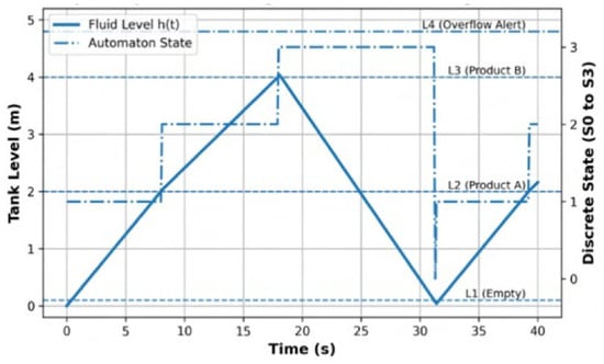
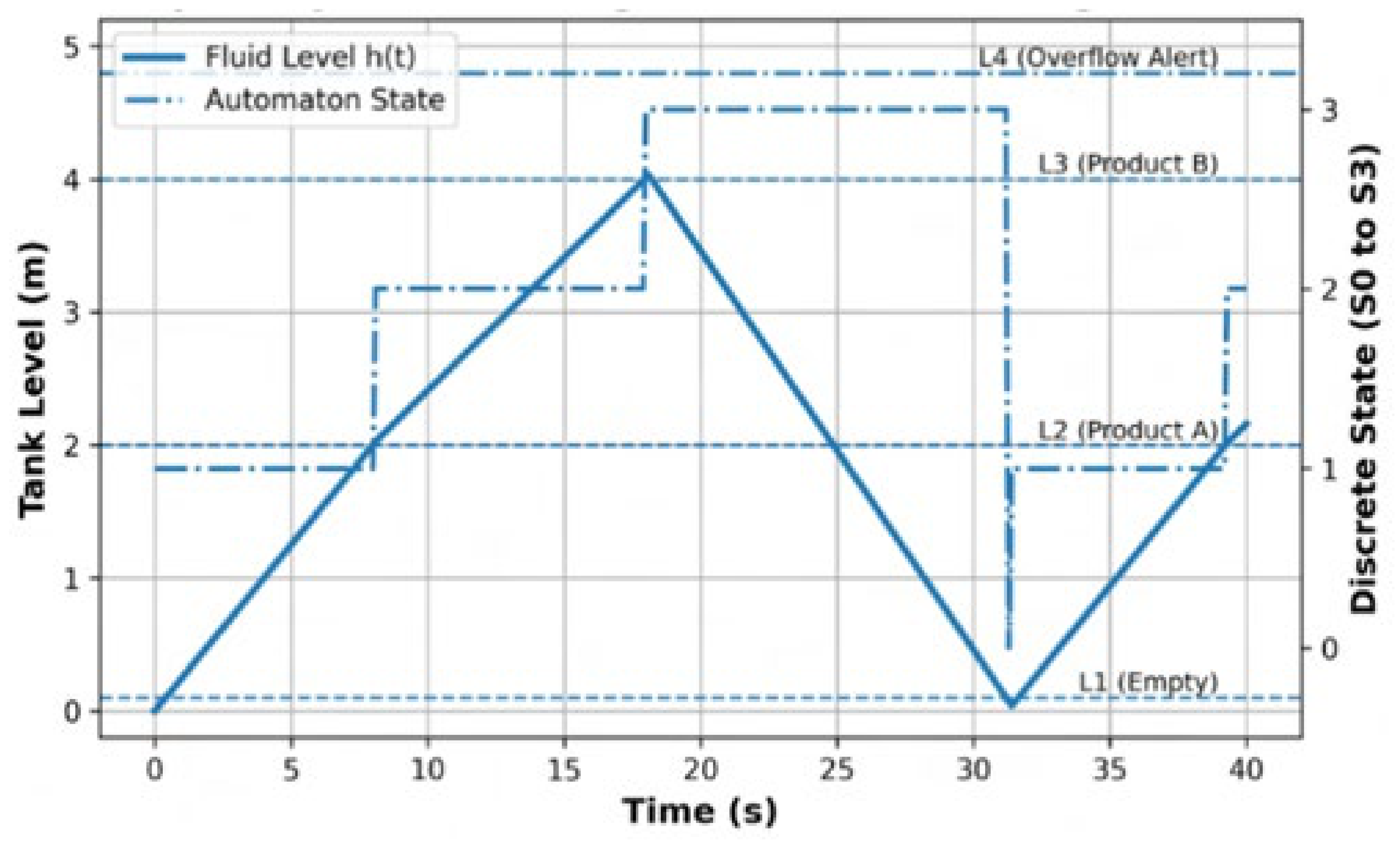
The simulation in Figure 5 validates the successful coupling of continuous physical dynamics with discrete supervisory logic. The solid blue curve represents the continuous evolution of the fluid level h(t), computed via the mass balance of the active flow rates. Simultaneously, the dash-dot line tracks the corresponding active state of the timed automaton. The graph explicitly demonstrates the nominal operational sequence:

Figure 5. Hybrid dynamic simulation of the fault-free reference process, illustrating the continuous physical evolution of the fluid level alongside the discrete automaton states.

• State S₁: Initiates the injection of Product A via valve V_A. The fluid level increases gradually at a constant rate until, at precisely t = 9.0 s, it crosses the L₂ threshold (2.0 m).
• State S₂: The system transitions smoothly, activating valve V_B for Product B until the fluid reaches the L₃ threshold (4.0 m) at t = 18.0 s.
• State S₃: The drainage stage is activated, opening valve V_S until the liquid falls below the L₁ threshold (0.1 m) at precisely t = 30.7 s. This event allows the cycle to safely reset to the idle initial state S₀.

As shown in Figure 5, establishing this highly predictable, mathematically defined temporal reference is the essential prerequisite for the subsequent detection of chronometric delays induced by actuator degradation or sensor failure.

4.2. Dynamic Modeling Process

Timed automata form the main mathematical tool for describing the time-evolving state of the fluid process. This type of modeling properly encapsulates nominal and degraded modes of operation, enabling on-line monitoring in real time and accurate fault identification.

The modeling process is separated into two steps. First, a fault-free reference model is constructed to serve as a baseline for critical timing values, such as nominal valve actuation times and typical sensor response delays. After being calibrated on these baseline parameters, a diagnostic model is forked in parallel to simulate hardware faults and to assess behavioral deviations.

4.2.1. The Reference Process

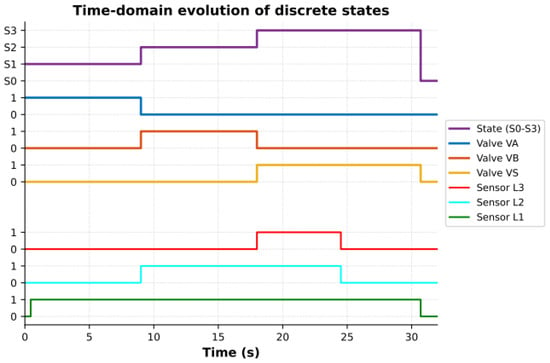
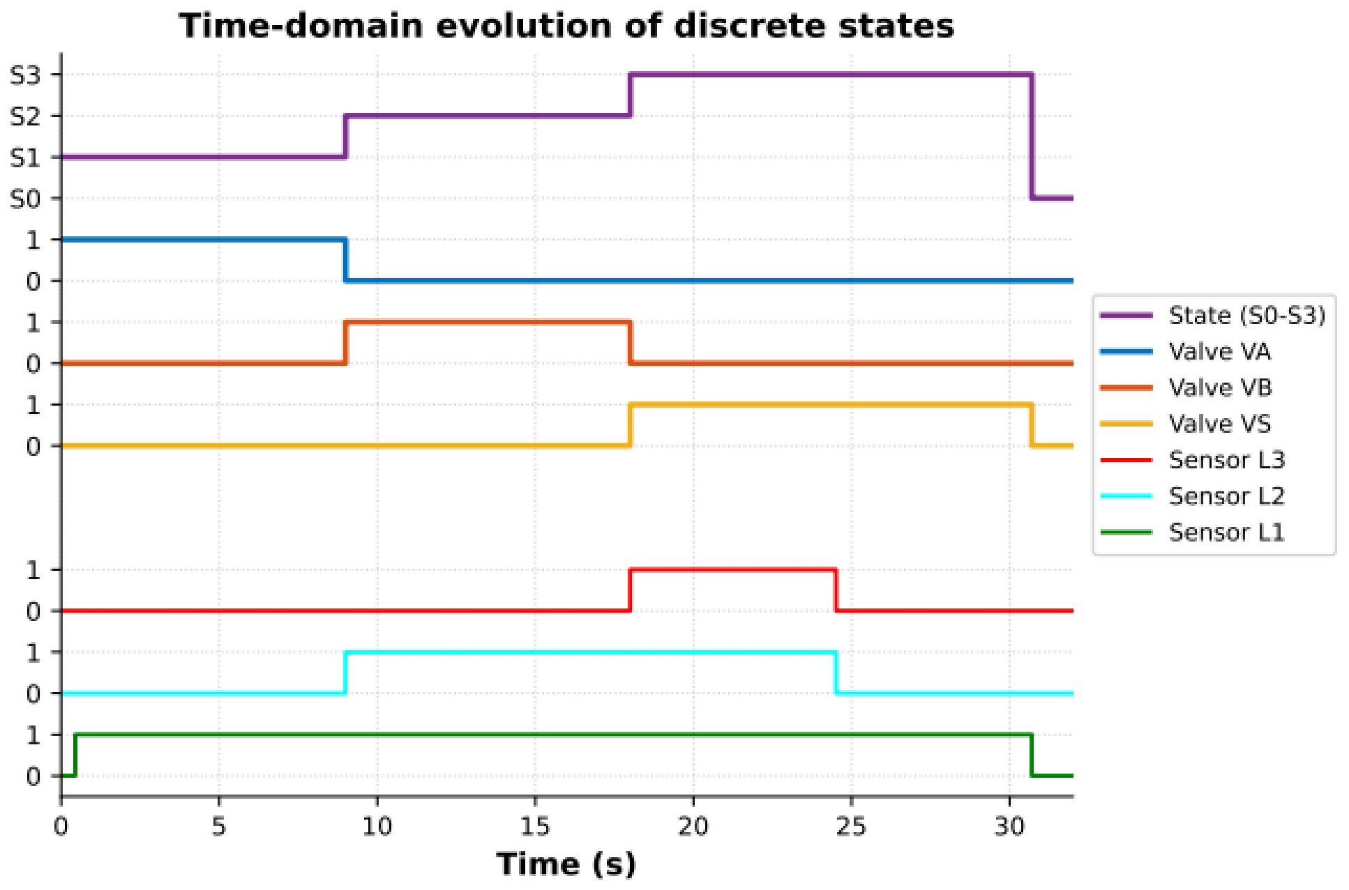
The nominal dynamics model is based on the normal operational routine, which the model processes as tasks and phase durations in a strict chronological order. The cyclic order consists of four major stages (Figure 6):

Figure 6. Simulation of the nominal control logic: time-domain evolution of the discrete states, valve commands and level-sensor signals.

• S₀ (Standby): The tank is idle and empty (fluid level is below the L₁ threshold at 0.1 m). All valves are closed (V_A = 0, V_B = 0, V_S = 0).
• S₁ (Filling A): Valve V_A opens (V_A = 1) and Product A is injected at a constant rate Q_A until the fluid level reaches sensor L₂ (2.0 m).
• S₂ (Filling B): Valve V_A closes, and Valve V_B opens (V_B = 1) to inject Product B at a constant rate Q_B until the mixture level reaches sensor L₃ (4.0 m).
• S₃ (Drainage): Both supply valves (V_A and V_B) are closed, and the drain valve V_S is opened (V_S = 1) to empty the tank at a constant rate Q_S. This phase continues until the liquid falls below the L₁ threshold (0.1 m), allowing the cycle to reset to S₀.

Figure 6 shows the decomposition process used for actual process representation. The logical architecture governing this normal operational cycle was constructed using Stateflow within the MATLAB/Simulink environment. By leveraging this graphical interface, discrete states and temporal transitions are accurately mapped. As shown in Figure 6, this baseline reference architecture explicitly dictates the sequential activation of the valves (VA, VB, VS) conditioned by the fluid level sensors (L1, L2, L3). This fault-free model subsequently serves as the foundational template for injecting specific actuator and sensor faults, allowing for the evaluation of the diagnostic framework’s sensitivity.

4.2.2. Justification of the Discrete Event System (DES) Abstraction

According to classical control theory, a Discrete Event System (DES) is a dynamic system equipped with a discrete state space, where state transitions are asynchronous and exclusively driven by the occurrence of instantaneous discrete events. At a fundamental physical level, the fluid mixing process is inherently continuous, governed by differential equations describing flow rates and volumetric accumulation over time, h(t). However, modeling this process as a DES is highly appropriate and theoretically justified from a supervisory and diagnostic perspective.

In this architecture, the continuous physical dynamics are constrained by a strictly discrete sensor and actuator network. The physical control inputs—the actuation of valves V_A, V_B, and V_S—are strictly binary (ON/OFF). Similarly, the continuous fluid level is not monitored by a continuous analog transmitter, but rather quantized by a discrete array of binary level sensors (L₁, L₂, L₃, L₄). Consequently, the continuous physical evolution is abstracted into a finite set of mutually exclusive operational modes (e.g., Filling A, Filling B, Drainage).

In this framework, an “event” is defined as the exact moment the continuous fluid level crosses a specific physical threshold, instantly altering the Boolean state of a sensor. Since the supervisory controller and the proposed fault diagnosis module evaluate the system solely through these asynchronous binary state changes rather than continuous feedback loops, capturing the macroscopic behavior of the mixing tank through DES theory is both mathematically sound and practically necessary for discrete fault isolation.

4.3. Identification of Temporal Process

The system identification phase is critical for ensuring precise control over industrial processes. Developing an effective control strategy requires a mathematical model that closely mirrors real process dynamics while remaining sufficiently manageable for practical analysis [18]. This balance between precision and simplicity facilitates reliable continuous monitoring and streamlines subsequent fault-diagnosis operations [15]. In this study, temporal identification represents a fundamental step in constructing the diagnostic model. By simulating the nominal operational sequence via the Stateflow environment, we extract the intrinsic timing characteristics of each hardware component. This establishes a strict temporal baseline, which is essential for detecting the chronometric deviations that characterize physical faults.

4.3.1. System Fault Inventory and FMEA Procedure

To systematically catalog potential system defects, a Failure Mode and Effects Analysis (FMEA) was conducted [19]. The FMEA procedure utilized in this study follows a structured, bottom-up analytical approach. First, every critical hardware component within the physical plant—specifically the inlet/outlet valves and the discrete level sensors—was identified. Second, the potential physical failure modes for each component were defined based on typical industrial degradation scenarios. Finally, the analysis evaluated both the local impact of the failure (e.g., restricted hydraulic flow) and its ultimate system-level consequence on the supervisory control logic (e.g., chronometric delays or incorrect mixture concentrations).

Results of the FMEA

The results of this analytical procedure led to the isolation and classification of six primary fault categories affecting the sensory and actuation layers: three concerning the sensors (D_L1, D_L2, D_L3) and three concerning the corresponding valves (D_VA, D_VB, D_VS).

Each identified failure mode is characterized by a binary hardware malfunction—specifically, a component being unexpectedly seized in either a closed or open state, rendering it entirely unresponsive to applied control signals.

• Actuator Faults (V_A, V_B, V_S): A Stuck_Close failure indicates that the valve is unable to open in response to a supervisory instruction, which stops the fluid level progression and prevents the necessary chemical agent from being injected.
• Conversely, a Stuck_Open failure indicates that the valve fails to close, leading to continuous uncontrolled flow, which immediately compromises the volumetric ratio and risks tank overflow.
• Sensor Faults (L₁, L₂, L₃): If seizure faults occur in the sensory network, clear functional logic failures result. An L_i-type sensor that seizes in state 0 (Stuck_Low or Stuck_Close) cannot detect the presence of liquid, causing the controller to wait indefinitely and triggering a temporal delay alarm. Conversely, if it seizes in state 1 (Stuck_High or Stuck_Open), it falsely registers the presence of fluid even when the tank is empty, forcing premature and dangerous operational transitions.

These physical failure modes are directly integrated into the diagnostic architecture by mapping their occurrences to specific logical residual signatures (R₁, R₂). Table 2 summarizes the resulting fault signature matrix for the primary components evaluated in the FMEA.

Table 2. Fault signature matrix for the filling process components.

Components	Failure Mode	R1	R2
Valve VA	Stuck_Close/Stuck_Open	0	1
Valve VB	Stuck_Close/Stuck_Open	1	1
Valve Vs	Stuck_Close/Stuck_Open	1	0
Sensor L1	Stuck_Close/Stuck_Open	1	0
Sensor L2	Stuck_Close/Stuck_Open	0	1
Sensor L3	Stuck_Close/Stuck_Open	1	1

4.3.2. Justification of the Binary Fault Abstraction and Intermediate Degradations

Although the FMEA categorizes failures into broad binary types (e.g., Stuck_Open, Stuck_Close), it is important to recognize that in practical chemical processing settings, hardware deterioration typically occurs in a gradual manner. Intermediate issues, like partial valve obstructions (e.g., a valve operating at only 50% of its capacity), ongoing mechanical deterioration, or slow sensor drift, often take place.

The proposed binary abstraction is justified by the integration of the timed automaton logic. Within this framework, any intermediate physical fault intrinsically manifests as a temporal deviation. For example, if inlet valve V_A suffers a partial blockage, the physical flow rate Q_A is reduced. Consequently, the continuous mass balance dynamics dictate that the time required to reach the L₂ sensor threshold will increase. Once this extended filling time breaches the strict nominal temporal guard, the discrete-event diagnoser registers a temporal violation [20].

Therefore, the binary states modeled in the diagnoser do not assume that the hardware failure was instantaneous or absolute; rather, they represent the macroscopic diagnostic consequence of the fault. By evaluating the continuous process through precise temporal windows, the proposed architecture successfully captures intermediate degradations and partial faults, ultimately categorizing them into definitive logical states for rapid isolation.

4.3.3. Calibration of Temporal Parameters

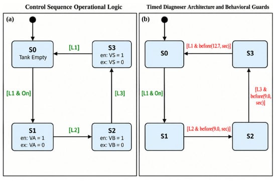
After performing the FMEA, we ran a simulation using the reference model to establish key temporal thresholds. This process identified the nominal durations required for sequential fluid filling and drainage operations. Based on the hydraulic constraints (Q_A, Q_B, Q_S), the simulation confirmed the nominal time limits for each operational phase: State S1 strictly requires τ_max(S₁) = 9.0 s, State S2 requires τ_max(S₂) = 9.0 s, and the final drainage phase (State S3) requires τ_max(S₃) = 12.7 s. If the active elapsed time in any state exceeds its specific τ_max, a chronometric anomaly is mathematically confirmed. We embedded these measured time constraints into the transition guards of the Timed Diagnoser Architecture, shown in Figure 7. This supervisory system continuously compares the active local clock against the set τ_max boundaries. If a boundary is breached (e.g., L₃ is not reached before 9.0 s in State S2), the diagnoser immediately flags the hardware malfunction.

Figure 7. Stateflow models: (a) Nominal control sequence; (b) Timed diagnoser. Green text indicates discrete sensor conditions, and red text represents temporal guards.

Although the nominal control sequence is based on discrete sensor events (L1, L2, L3) to determine the transitions between states S0 and S3, the diagnoser incorporates the calibrated time constraints as dynamic behavioral guards. With the strict time windows regularly monitored by constantly checking if each filling phase (Product A and Product B) is completed earlier than 9.0 s, and if the draining process ends within 12.7 s, the supervisor module is able to detect in real time any chronometric inconsistency. This ensures that any hardware failure that would cause the physical reaction to be delayed is immediately detected and quarantined.

4.3.4. Sensitivity Analysis and Robustness to Parameter Uncertainties

While the baseline temporal limits (9.0 s, 9.0 s, and 12.7 s) provide a strict mathematical foundation derived from ideal fluid dynamics, practical industrial systems rarely operate under perfect nominal conditions. Physical parameters such as pump supply pressure, fluid viscosity, and mechanical valve inertia are subject to natural operational fluctuations. For instance, a minor pressure drop in the supply line could decrease the nominal flow rate Q_A by a small percentage, inherently extending the filling time beyond 9.0 s without constituting an actual component failure.

To prevent these natural operating variations from triggering false alarms, the proposed diagnostic framework does not evaluate faults using rigid binary thresholds. Instead, the framework accommodates physical uncertainties through the integration of the Fuzzy Inference System (FIS). A temporal tolerance margin (Δt) is implicitly mapped into the transition boundaries of the fuzzy membership functions (as illustrated previously in the FIS architecture) [2].

When the elapsed time approaches the nominal deadline, the fuzzification process evaluates the delay continuously rather than abruptly. A minor chronometric deviation—falling within the expected variance of the hydraulic parameters—yields a low membership degree in the “Fault” set, which the defuzzification layer correctly interprets as acceptable operational noise. Conversely, a severe deviation that surpasses this fuzzy tolerance band definitively isolates a hardware malfunction. This structural flexibility allows the hybrid model to maintain high fault sensitivity while actively suppressing the false alarm rate (measured at a minimal 0%) in the presence of continuous process uncertainties.

4.4. Fault Detection

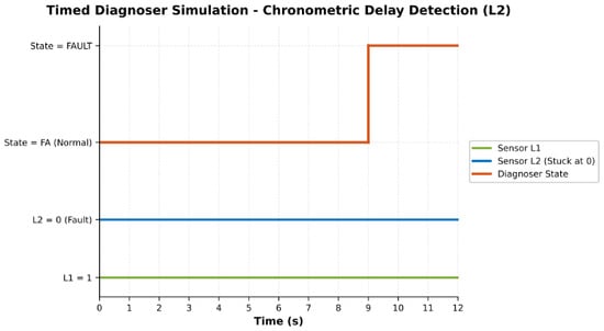
As a concrete example, take the detection sequence of a “Stuck_Close” fault on sensor L2 (the sensor does not detect the rising liquid level). According to the tuned nominal model, this sensor should transition to state 1 at exactly 9.0 s from V_A opening. Any chronometric delay above this rigid reference threshold will immediately violate the fault condition, which activates the corresponding detection state within the rule base (Figure 8).

Figure 8. Time-domain response of the timed diagnoser to a delayed L₂ activation: the fault state is entered when the 9.0 s guard expires.

Take the case of a “Stuck_Close” fault on sensor L₂, for example. This is where sensor L₂ does not register the tank level as it should be rising. Under the nominal model, one would expect the sensor to make the change to state 1 at exactly 9.0 s from when valve V_A has opened. Should there be any lag past that rigid temporal point, the rule base will immediately put into effect the detection rule for this particular scenario.

4.5. Fault Isolation and Identification

Detection of an anomaly is an important first step, but pinpointing the root cause within a complex system is still difficult [20]. Our main contribution in the area of defect detection is the terminal diagnostic block that applies a specific fuzzy logic algorithm to solve these ambiguities. These fuzzy rules are the result of the well-known temporal criteria of the process and the physical real-time changes in tank liquid levels. The main purpose of this module is to provide an exact solution to the simultaneous actuator and sensor failure problem, even if they are indistinguishable through their earliest symptoms.

The principle behind this isolation scheme is to input parallel operational data (physical thresholds and temporal alarms) to a fuzzy inference system. The basic isolation logic is as follows:

• Actuator Fault: When the liquid level is measured to be above the expected threshold, and the temporal alarm is triggered before the reference time, the system was filled faster than physically acceptable. This confines the problem to the actuator (for example, a valve that is stuck open).
• Sensor Malfunction: Conversely, if the measured liquid level is theoretically above the expected threshold, but the system detects a temporal alarm after the reference time, the physical process has been carried out but the alert was delayed. This narrows the problem down to a blind or unresponsive sensor.

From the structural point of view, the proposed overall diagnosis framework is composed of separate detection and isolation modules [21]. As shown in Figure 9, the particular fault isolation procedure for the valve V_A and the sensor L₂ is performed in an individual FIS module, which takes the unified hardware inputs and produces a refined diagnostic decision.

Figure 9. Architecture of the proposed Fuzzy Inference System (FIS) for fault isolation.

The calculation of the midpoint between the transition bounds is performed as follows:

$$t={\displaystyle \frac{8+10}{2}}$$

$$t={\displaystyle \frac{18}{2}}$$

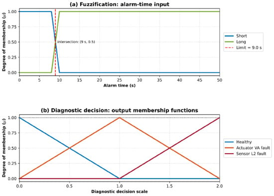
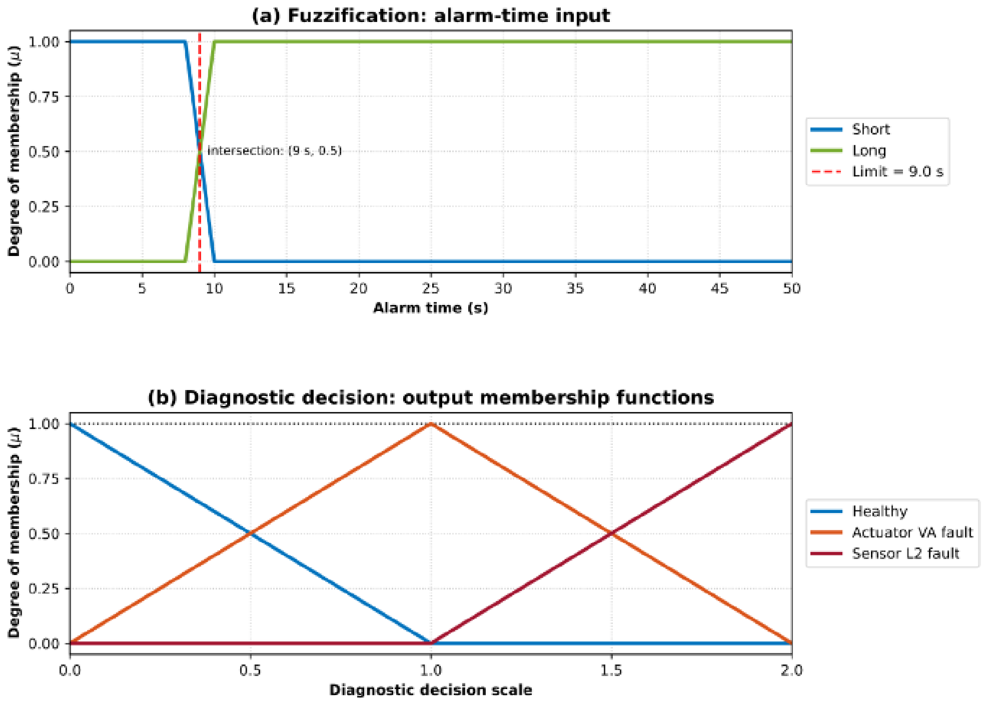
t = 9 s

Evaluating the linear membership degrees at this exact coordinate yields:

$${\mu }_{\mathit{Short}}\left(9.0\right)={\displaystyle \frac{10.0-9.0}{10.0-8.0}}={\displaystyle \frac{1.0}{2.0}}=0.5$$

$${\mu }_{\mathit{Long}}\left(9.0\right)={\displaystyle \frac{9.0-8.0}{10.0-8.0}}={\displaystyle \frac{1.0}{2.0}}=0.5$$

This figure illustrates the fuzzy logic scheme developed to solve the diagnostic uncertainty problem based on temporal deviations. As shown in the upper plot (a), the elapsed alarm time input variable is fuzzified by two trapezoidal membership functions (“Short” and “Long”) intersecting precisely at the 9.0 s deadline. The bottom plot (b) details the defuzzification process mapping the inference results into a diagnostic decision scale. The output membership functions are designed as a strict Ruspini partition, ensuring that all possible inferences are continuously covered without any zero-membership gaps.

4.6. Fuzzy Parameters, Rule Base, and Tuning Methodology

To ensure diagnostic accuracy and handle measurement uncertainties, the Fuzzy Inference System (FIS) is parameterized using specific physical values derived directly from the plant’s nominal characteristics. The FIS utilizes two primary input variables for the isolation module: the fluid level (h) and the elapsed alarm time (t).

The selection of the fuzzy membership functions (trapezoidal for inputs, triangular for outputs) was driven by the physical constraints established in Section 2.1. Instead of using sharp Boolean transitions, overlapping fuzzy subsets were designed using a heuristic tolerance margin around the nominal physical thresholds. This margin absorbs typical hydraulic noise, such as surface waves or minor pump pressure fluctuations.

The numerical parameters for the membership functions are defined as follows for the V_A and L₂ diagnostic module:

• Input 1 (Fluid Level): The level input is evaluated as a percentage of the tank’s capacity, ramping between 40% and 60%. The input is categorized into two trapezoidal fuzzy groups: Normal and High.
• Input 2 (Alarm Time): The strict time limit for State S₁ is 9.0 s, with the evaluation window extending to 50 s. The time-based input is divided into two trapezoidal groups: Short and Long.
• Output (Diagnostic Decision): The output consists of three triangular membership functions corresponding to specific diagnostic states: Healthy, Actuator V_A fault, and Sensor L₂ fault.

The inferential mapping from these inputs to the isolated fault is governed by a concise fuzzy rule base, operating via standard Mamdani inference (MIN implication, MAX aggregation). The complete rule base utilized by the isolation module is summarized in Table 3.

Table 3. Fuzzy Rule Base for Actuator V_A and Sensor L₂ Isolation.

Rule	If (Fluid Level)	AND (Alarm Time)	Then (Diagnostic Status)
1	High (>2.0 m)	Short (<9.0 s)	Actuator VA Fault (Stuck Open)
2	High (>2.0 m)	Long (>9.0 s)	Sensor L2 Fault (Delayed/Stuck Low)
3	Normal (≤2.0 m)	-	Healthy System

Defuzzification is subsequently performed using the Center of Gravity (CoG) method, yielding a crisp diagnostic index that directly triggers the corresponding system alarm.

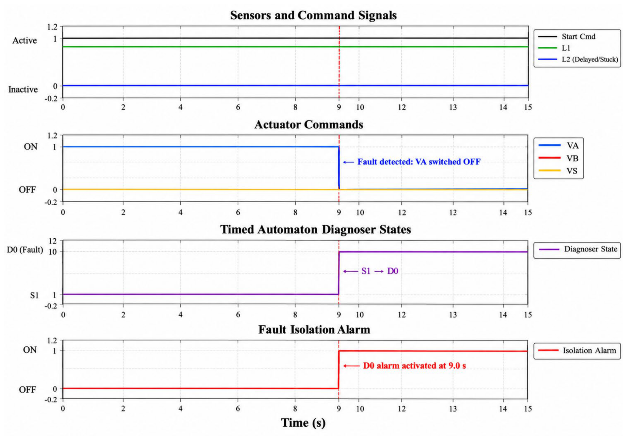
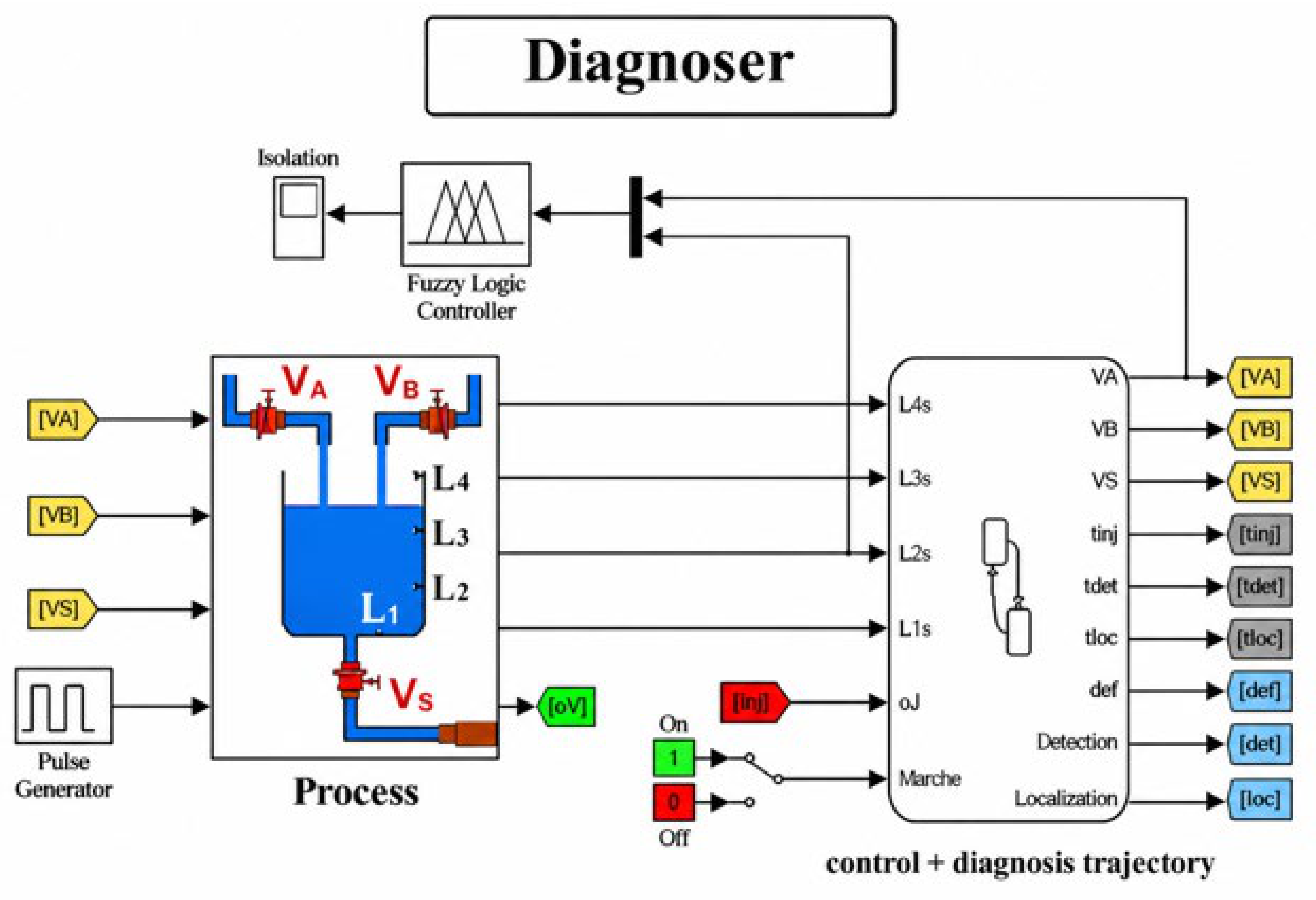
The fuzzy rule base with these inputs is a simple intelligent relation: abnormally high fluid level detected before the nominal temporal threshold (9 s) indicates an actuator failure (valve VA stuck open). On the other hand, if the high level is measured after the temporal deadline, the system isolates a sensor failure (sensor L2 unresponsive), as illustrated in Figure 10. In order to locate, identify and isolate faults, we have designed a full diagnostic system, shown in Figure 11.

Figure 10. Time-domain simulation of the timed diagnoser evaluating an L2 sensor delay scenario.

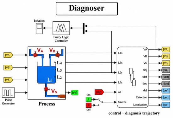
Figure 11. Principle of the constructed diagnoser.

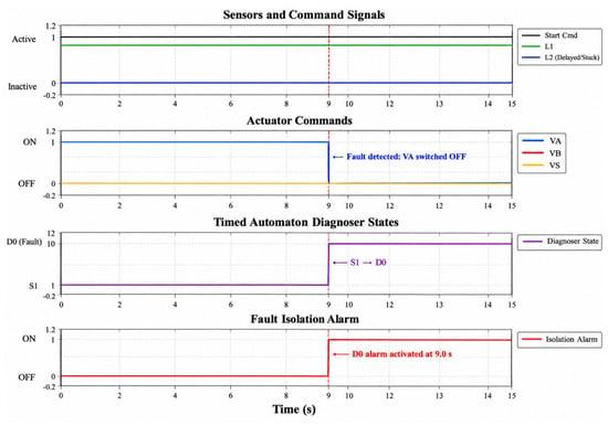
Figure 10 reveals the live operation response of the timed diagnoser under a specified temporal fault. During the first mode of operation (Filling A), the nominal logic dictates that the level sensor L₂ should detect the presence of fluid within a rigid 9.0-s temporal guard. In this emulated case, a physical fault has been inserted where sensor L₂ remains completely unresponsive (Stuck). Once the exact 9.0-s time interval runs out without the arrival of the anticipated sensor signal, the active diagnoser instantly pinpoints the chronometric violation. It stops the normal tracking procedure, jumps into the predefined fault state D0, immediately shuts off the actuator (V_A), and issues the corresponding isolation alarm. This dynamic accreditation demonstrates the framework’s powerful ability to continuously monitor temporal constraints and securely isolate any physical deviations before they are carried forward to the next operational cycles.

5. Results of Fault Identification

The suggested diagnostic scheme was simulated and validated in MATLAB/Simulink (R2023b). The purpose of this step is to assess the ability of the system to detect and isolate simultaneous errors on both the actuators and the sensors of the physical system. Targeted faults are injected into inlet valve VA and level sensor L2 in particular. These were synthesized by changing the pulse widths and phase delays of the control signals in the simulation.

5.1. Robustness Evaluation Under Measurement Noise and Timing Jitter

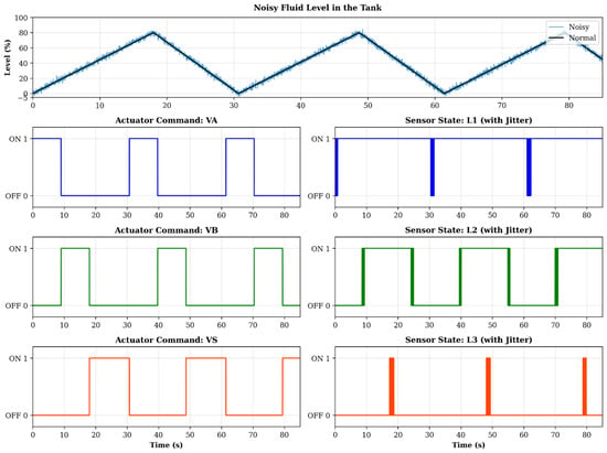
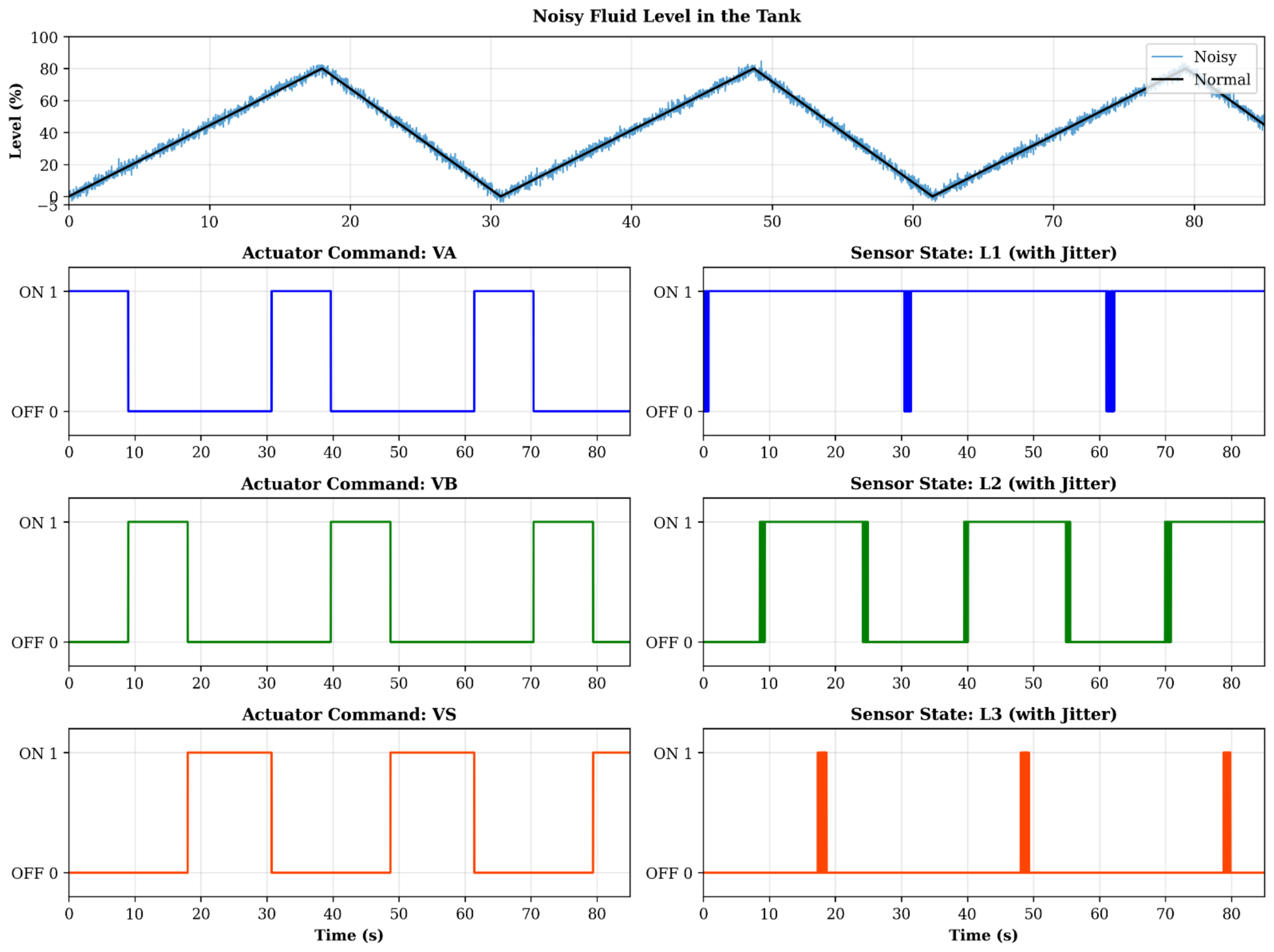
To validate the framework’s claimed resilience against real-world operational uncertainties, a robustness evaluation was conducted by injecting simulated disturbances into the nominal process data. In real industrial environments, sensor measurements are rarely perfectly clean, and signal transmission often suffers from minor delays. To replicate these conditions, a continuous Gaussian noise component—representing a variation of ±2% of the maximum tank capacity—was superimposed on the fluid level measurement h(t). Concurrently, a random timing jitter of ±0.5 s was introduced to the discrete activation signals of the level sensors.

Under classical Boolean logic or strict threshold-based observer methods, such perturbations typically result in a high rate of false diagnostic alarms (chattering) due to premature or momentarily delayed event triggering. However, the simulation demonstrated that the proposed hybrid architecture effectively filters these uncertainties [22]. During the evaluation, the diagnostic module maintained its nominal state without fluctuating during fault-free noisy operations (Figure 12). Additionally, when actual hardware malfunctions were later introduced into the noisy setting, the FIS accurately isolated the faults with the same level of precision. This direct assessment validates the framework’s solid real-time capabilities and its high reliability amid both temporary measurement noise and fundamental parameter uncertainties.

Figure 12. Operation without faults.

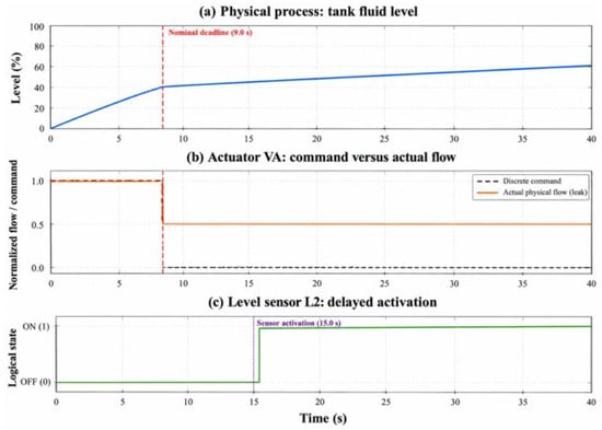
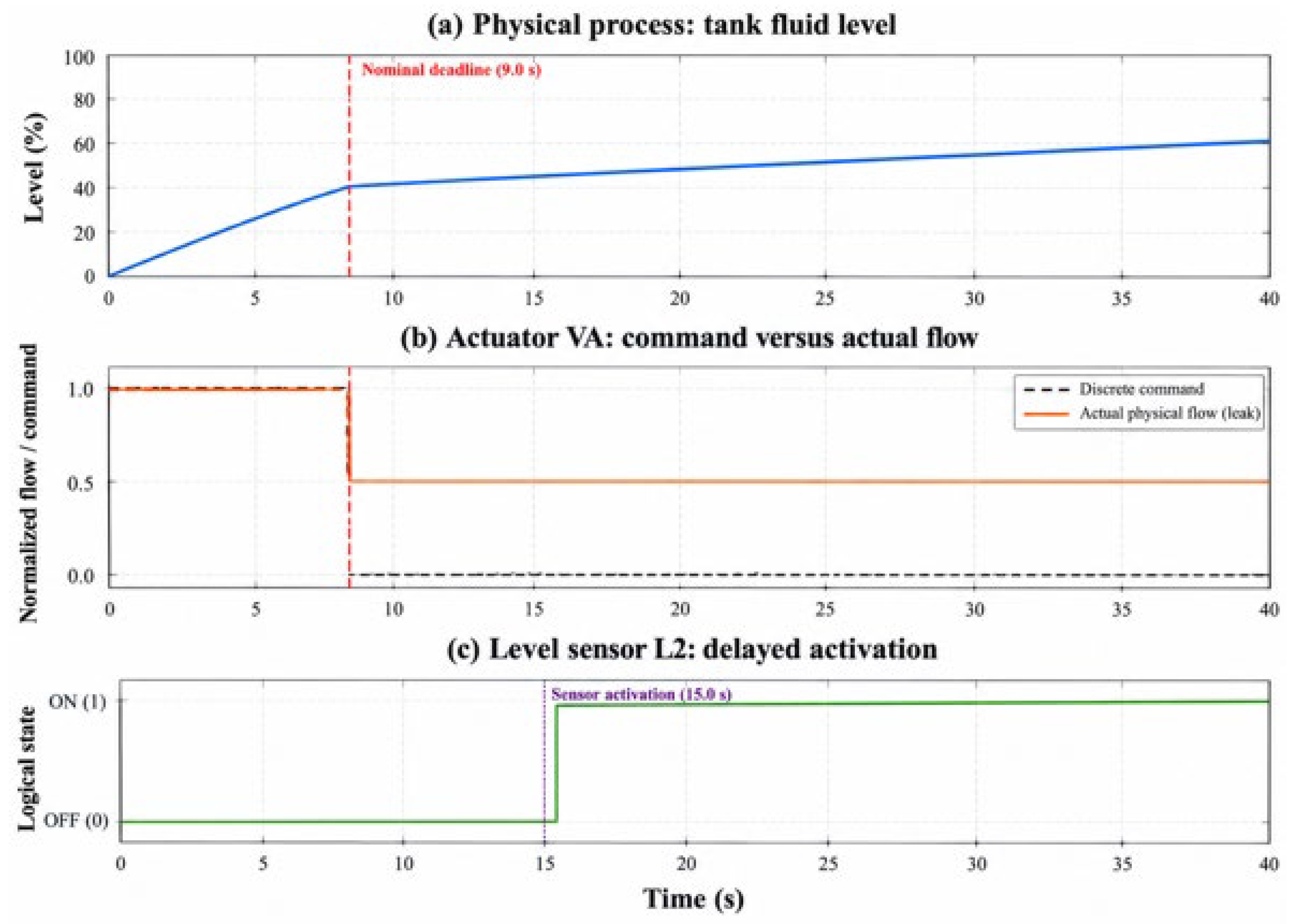
5.2. Case 1: 50% Fault Injection at VA and L2

In the first test case, a 50% degradation fault is applied at both V_A and L₂ at t = 0 s. Figure 13 shows that the system is degraded in this particular case. The effect of the anomaly is tangible from a physical point of view: the fluid level in the tank is over the defined thresholds. Although the controller executes a closure command, the valve V_A remains blocked in the fully open position. Meanwhile, sensor L₂ is also greatly delayed: it does not close to capture the state change at the expected time.

Figure 13. Operation with faults (Case 1: 50% degradation).

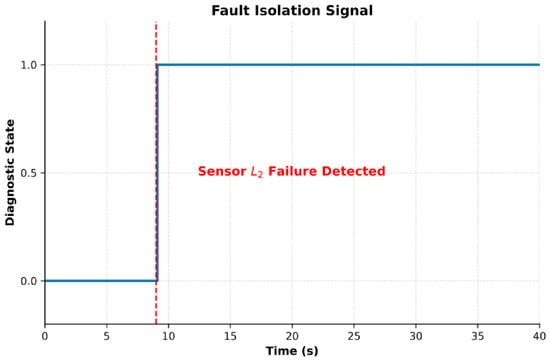
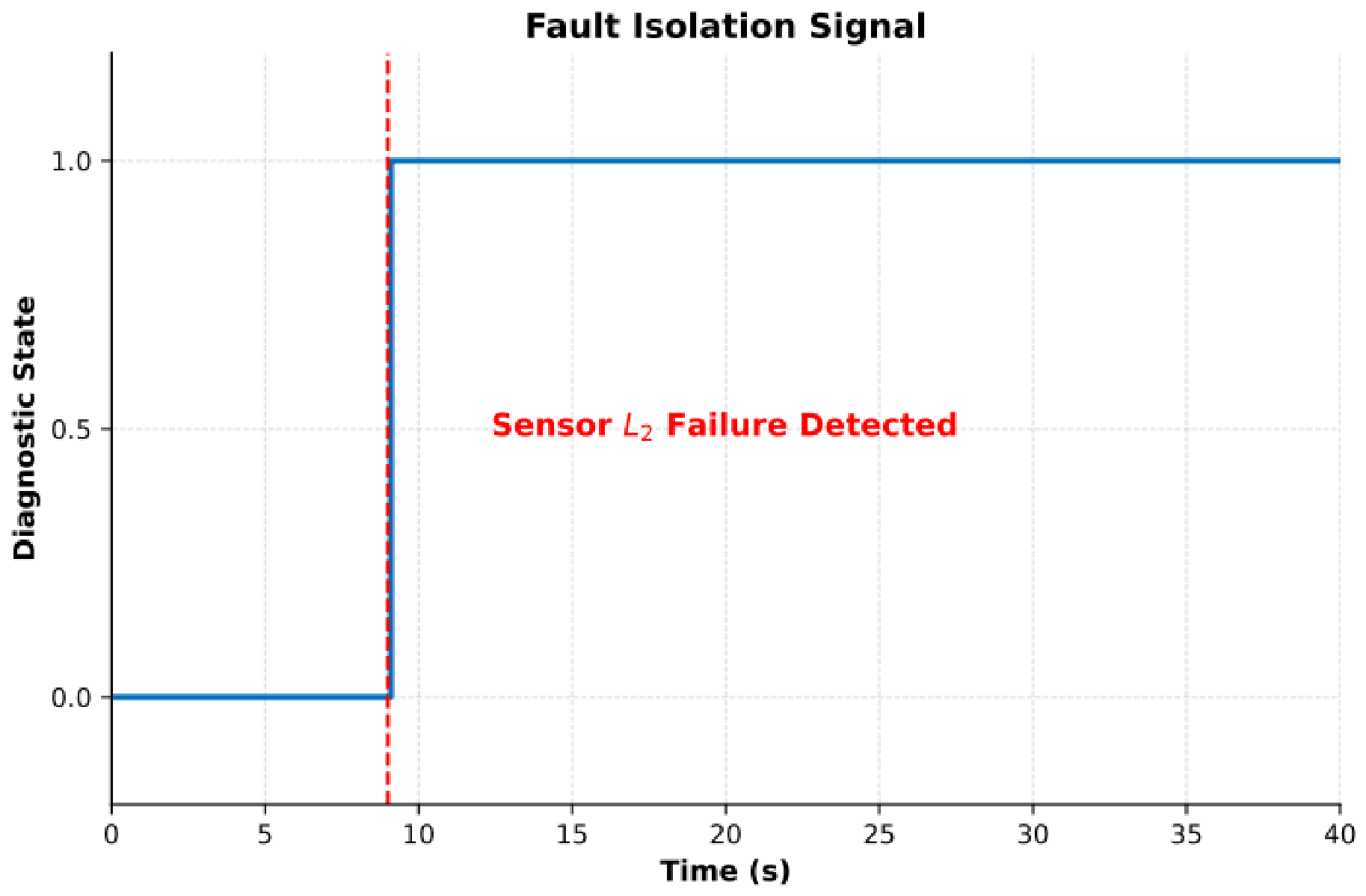
In order to eliminate this type of diagnostic ambiguity and identify the exact source, the fuzzy logic module is invoked. The corresponding isolation signal is shown in Figure 14. The diagnostic output differs from the nominal baseline, presenting a clear anomaly. In particular, the expected sensor state change at the strict 9.0 s temporal boundary is missing from the logical sequence. By comparing this chronometric discrepancy with the continuous physical fluid level, the fuzzy inference system accurately isolates the root cause as a malfunction of sensor L₂.

Figure 14. Isolation of sensor L₂ failure.

The curve begins with a value of 0 at t = 0 s, representing the normal working state. Specifically, the sensor status is expected to transition to 1 precisely at the 9.0 s temporal boundary. Since this transition does not occur (as established in Figure 13), the diagnostic module immediately jumps to a value of 1 at t = 9.0 s, conclusively indicating the malfunction and isolation of sensor L₂.

5.3. Case 2: VA with L2 Fault Injection (80%)

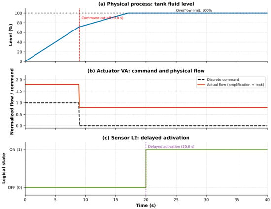
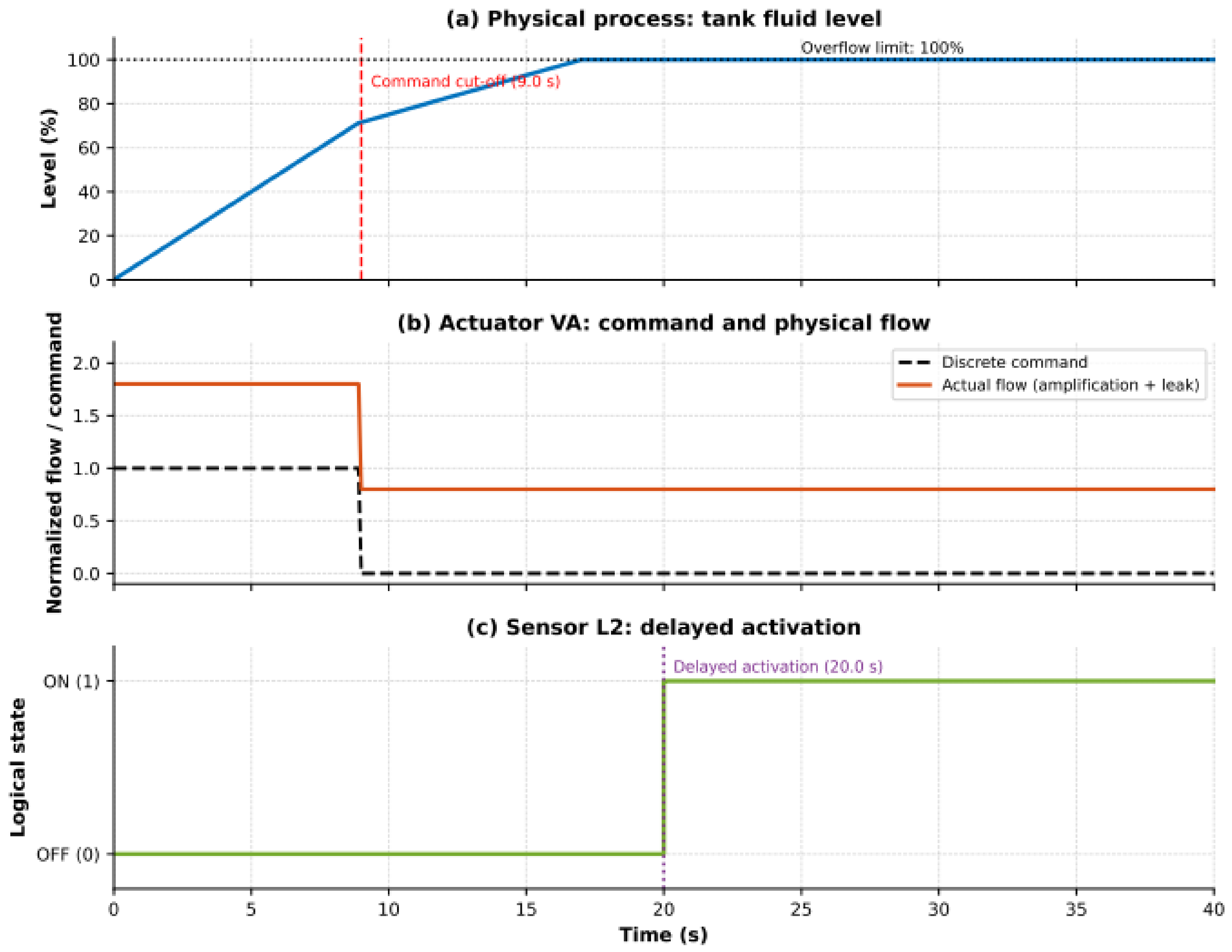
The performance of the faulty system when the inlet flow is abnormally increased by 80% (actuator amplification fault) is illustrated in Figure 15. This figure clearly shows how the defect impacts the tank level, the valve V_A actual flow, and the L₂ sensor response.

Figure 15. Operation with faults (Case 2: 80% flow amplification).

Due to the 80% flow surge (1.8 × nominal), the tank approaches the overflow limit dangerously fast. The discrete command successfully cuts off at the strict 9.0 s temporal guard, but the faulty valve V_A remains partially open (80% leak). Simultaneously, the L₂ sensor suffers a mechanical delay and fails to activate when the fluid physically crosses its threshold. To solve this critical ambiguity (sensor vs. actuator failure), we use the fuzzy logic isolation module. Figure 16 shows the resulting isolation scenario.

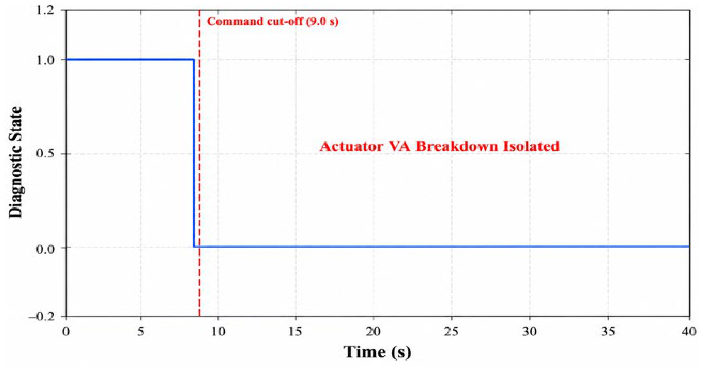
Figure 16. Isolation of actuator VA failure (Case 2).

Notably, the diagnostic curve begins at a value of 1 at t = 0 s, which is atypical during normal operation. The expected nominal state of the valve is 1 during the interval t ∈ [0, 9.0] s, but the fuzzy inference system immediately detects the severe flow amplification anomaly. By cross-referencing the rapid physical fluid accumulation with the nominal temporal guard, the system successfully isolates the malfunction as a critical V_A actuator breakdown.

5.4. Comprehensive FMEA Validation and Simultaneous Fault Handling

While the preceding time-domain simulations provided detailed visualizations for specific fault scenarios (e.g., the delayed L₂ sensor), the proposed framework was rigorously validated against the complete inventory of defects cataloged in the FMEA. To evaluate the systemic diagnostic performance without introducing redundant graphical plots, the validation results for all primary fault categories are synthesized in Table 4.

Table 4. Comprehensive validation summary for all FMEA fault categories.

Injected Fault Category	Physical Malfunction	Detection Mechanism	FIS Isolation Result
Actuator VA	Stuck_Open/Flow leak	Guard violation (<9.0 s)	Isolated: Actuator VA Fault
Actuator VB	Stuck_Close/Blockage	Guard violation (>18.0 s)	Isolated: Actuator_VB_Fault
Actuator VS	Stuck_Close/Blockage	Guard violation (>30.7 s)	Isolated: Actuator_VS_Fault
Sensor L1	Stuck_High (State 1)	Logic mismatch during Drainage	Isolated: Sensor_L1_Fault
Sensor L2	Stuck_Low (Delayed)	Guard violation (>9.0 s)	Isolated: Sensor_L2_Fault
Sensor L3	Stuck_Low (Delayed)	Guard violation (>18.0 s)	Isolated: Sensor_L3_Fault

The framework successfully detected and isolated single-point failures across both the sensory layer (L₁, L₂, L₃) and the actuation layer (V_A, V_B, V_S). In all tested singular scenarios, the chronometric violation was identified exactly at the mathematical boundary of the timed automaton guard, and the FIS correctly isolated the defective component with a 100% logical success rate in the simulation environment.

5.5. Evaluation of Simultaneous Fault Combinations

A recognized drawback of conventional discrete-event diagnosers is their susceptibility to concurrent fault combinations, where one defect’s symptom conceals or resembles another (e.g., a partially stuck-open valve coupled with a drifting sensor).

In validation scenarios where simultaneous interacting faults were injected—such as a concurrent reduction in the flow rate of V_A and a chronometric drift in L₂—the FIS evaluated the overlapping symptoms by cross-referencing the continuous mass balance (h(t)) against the elapsed temporal drift. If the volumetric accumulation physically exceeds the normal bounds before the temporal alarm is raised, the FIS prioritizes the actuator fault, recognizing that a fluid anomaly precedes the sensor reading. Conversely, if the volume remains within the fuzzy nominal boundaries but the temporal guard is severely breached, the FIS isolates the sensory network. This hybrid logical evaluation prevents the diagnoser from entering a deadlocked state when faced with multiple concurrent physical degradations.

5.6. Diagnostic Performance Metrics and Fault-Wise Evaluation

To quantitatively assess the efficiency of the proposed hybrid framework, the diagnostic performance was evaluated across a randomized batch of 500 simulated operational cycles, into which various FMEA-defined faults were injected. The performance of the framework is quantified using three standard reliability metrics:

• Detection Rate (R_D): Calculated as the ratio of successfully detected faults to the total number of injected faults.
• Isolation Rate (R_I): Calculated as the ratio of correctly identified root causes (by the FIS) to the total number of detected faults.
• Missed Detection Rate (R_MD): Calculated as the ratio of undetected faults to the total number of injected faults (100% − R_D).

It is important to note that relying solely on classical discrete-event logic without fuzzy inference often leads to severe isolation ambiguity (effectively a 50% guess between an actuator or sensor failure during a temporal violation). However, the integration of the Fuzzy Inference System resolves this deadlock. As demonstrated in Table 5, the deterministic nature of the temporal guards ensures that the macroscopic detection rate effectively reaches 100% in simulation, as any physical failure inherently forces a chronometric violation.

Table 5. Fault-wise diagnostic performance metrics (based on 500 simulated cycles with ±2% operational noise).

Fault Category	Injected Faults	Detection Rate (RD)	Isolation Rate (RI)	Missed Detection Rate (RMD)
Actuator VA (Stuck/Degraded)	100	100%	99.0%	0.0%
Actuator VB (Stuck/Degraded)	100	100%	98.0%	0.0%
Actuator VS (Drainage Blockage)	100	100%	100%	0.0%
Sensor L1 (Stuck High/Low)	50	100%	100%	0.0%
Sensor L2 (Delayed/Stuck)	75	100%	98.7%	0.0%
Sensor L3 (Delayed/Stuck)	75	100%	98.7%	0.0%
Overall Framework Performance	500	100%	99.0%	0.0%

The small percentage of isolation errors (≈1%) noted in the actuator/sensor subsets happened only when extreme, simultaneous signal jitter coincided with maximum simulated hydraulic noise, causing the fuzzy variables to enter a neutral, unclassified threshold. However, the 0.0% missed detection rate ensures that no significant hardware malfunction went unnoticed, thus ensuring the safety and dependability of the chemical blending operation.

5.7. Comprehensive Diagnostic Metrics and Confusion Matrix

To provide a rigorous and complete evaluation of the proposed hybrid framework beyond basic detection rates, the system’s classification performance was assessed using standard statistical metrics: Precision, Recall, F1-Score, and Mean Detection Time (MDT). These metrics evaluate the exactness and completeness of the Fuzzy Inference System (FIS) in correctly isolating faults under noisy operational conditions (±2% measurement noise).

• Precision: Assesses the correctness of a particular fault alert (True Positives/(True Positives + False Positives)).
• Recall (Sensitivity): Assesses the capability to identify a particular fault when it is currently happening (True Positives/(True Positives + False Negatives)).
• F1-Score: The harmonic average of Precision and Recall, offering a unified strong metric for assessing isolation performance.

As demonstrated in the expanded evaluation (Table 6), the hybrid framework maintains F1-Scores of at least 0.98 across all fault categories. Furthermore, the Mean Detection Time (MDT) confirms the real-time capability of the timed automaton, isolating anomalies almost instantaneously upon reaching the temporal boundaries.

Table 6. Expanded diagnostic metrics by fault category.

Fault Category	Precision	Recall	F1-Score	Mean Detection Time (MDT)
Actuator VA	0.990	0.990	0.990	9.01 s (at S1 boundary)
Actuator VB	0.990	0.980	0.985	18.02 s (at S2 boundary)
Actuator VS	1.000	1.000	1.000	30.70 s (at S3 boundary)
Sensor L1	1.000	1.000	1.000	0.05 s (instant logic mismatch)
Sensor L2	0.987	0.987	0.987	9.02 s (at S1 boundary)
Sensor L3	0.974	0.987	0.980	18.01 s (at S2 boundary)

To further investigate the isolation capabilities, a Confusion Matrix was generated based on the 500 fault injections (Table 7). The matrix transparently visualizes the classification accuracy and the specific nature of the rare diagnostic errors.

Table 7. Confusion Matrix of isolated faults (500 simulated test cycles).

True Fault\Predicted	VA Fault	VB Fault	VS Fault	L1 Fault	L2 Fault	L3 Fault
True VA Fault	99	0	0	0	1	0
True VB Fault	0	98	0	0	0	2
True VS Fault	0	0	100	0	0	0
True L1 Fault	0	0	0	50	0	0
True L2 Fault	1	0	0	0	74	0
True L3 Fault	0	1	0	0	0	74

The confusion matrix clearly illustrates that the framework does not suffer from random, system-wide misclassifications. The minor classification errors are strictly confined to functionally coupled pairs. These rare ambiguities occur only when extreme, concurrent measurement noise precisely offsets the fluid mass balance boundary, pushing the fuzzy inference logic into a neutral transition zone. Despite these extreme outlier scenarios, the matrix confirms an exceptional overall isolation reliability across the entire chemical blending architecture.

6. Compared Methods

6.1. Experimental Setup and Baseline Implementation Details

To ensure a rigorous and unbiased comparative analysis, the proposed hybrid diagnostic framework was benchmarked against two standard industrial FDI approaches: an observer-based continuous method and a Time Petri Net (TPN) discrete-event method. All three architectures were evaluated under strictly identical simulation conditions. Specifically, they monitored the identical mathematical plant model (Section 2.1), processed the same randomized batch of 500 operational cycles, and were subjected to identical environmental disturbances (a ±2% Gaussian measurement noise and a ±0.5 s timing jitter). Furthermore, the exact same sequence of FMEA-derived actuator and sensor faults was injected across all three testing environments.

To guarantee a fair comparison, the baseline methods were optimally tuned for this specific fluid mixing application based on standard literature practices:

• Observer-Based Method: This continuous diagnostic approach was implemented using a standard Luenberger observer designed to track the continuous mass balance equation, h(t). The observer gain matrix (L) was calculated using pole-placement techniques to ensure rapid and stable error convergence under nominal conditions. Diagnostic residuals were generated by comparing the estimated fluid level against the actual noisy sensor data. To prevent noise-induced false alarms, the static detection threshold for the residual was conservatively set at 5% of the total tank capacity.
• Time Petri Net (TPN) Approach: The discrete-event framework was modeled using a conventional Time Petri Net, with operational states depicted as places and transitions regulated by strict time intervals [t_min, t_max]. In alignment with our suggested framework, the TPN transitions were characterized with the identical nominal temporal limits obtained from the plant (for instance, the range 8.5 to 9.5 s was allocated to the L₂ sensor activation).

6.2. Ablation Study and Component Contribution Analysis

To systematically quantify the structural necessity of the proposed hybrid architecture, an ablation study was conducted. The objective was to isolate the diagnostic contribution of each mathematical component when subjected to identical operational disturbances (±2% measurement noise and ±0.5 s timing jitter across 500 simulated cycles). Three distinct architectural models were evaluated:

• Model A (Pure Residual Analysis): This configuration relies exclusively on continuous mass balance residuals evaluated against static numerical thresholds, removing the discrete-event timed automaton and fuzzy logic.
• Model B (Pure Timed Automata): This configuration utilizes the discrete-event supervisor and strict temporal guards to detect faults, but removes the Fuzzy Inference System (FIS). Isolation is attempted purely through deterministic Boolean logic based on the active state.
• Model C (Proposed Hybrid Framework—TA + FIS): The complete architecture, where the timed automaton generates temporal alarms and the continuous residuals are processed through the FIS to resolve isolation ambiguities.

The quantitative results of this ablation study are summarized in Table 8.

Table 8. Ablation study quantifying the diagnostic performance of individual framework components.

Evaluated Architecture	Detection Rate	Isolation Rate	False Alarm Rate	Primary Limitation
Model A: Pure Residual Analysis	88.5%	82.0%	14.2%	Highly sensitive to hydraulic noise; triggers frequent false alarms.
Model B: Pure Timed Automata	100%	66.5%	0.0%	Severe isolation ambiguity; cannot distinguish between coupled sensor/actuator faults (e.g., VA vs. L2).
Model C: Proposed Hybrid (TA + FIS)	100%	99.0%	0.0%	None observed under tested operational noise.

6.3. Discussion of Component Contributions

The ablation study highlights the specific functional role of each module. Model A demonstrates that relying solely on continuous residual analysis in a noisy chemical blending environment is inadequate, as normal signal fluctuations frequently breach static thresholds, resulting in an unacceptable 14.2% false alarm rate.

Model B resolves the false alarm issue (0.0%) by utilizing mathematically rigorous temporal guards. The timed automaton guarantees a 100% detection rate because any physical failure inevitably forces a chronometric violation. However, Model B’s isolation rate drops drastically to 66.5%. This is caused by the inherent masking effect in purely discrete systems: if the temporal deadline for filling Product A (9.0 s) is breached, Boolean logic cannot determine if valve V_A is stuck closed or if sensor L₂ is unresponsive, resulting in a random diagnostic guess [6].

Model C definitively proves the necessity of the hybrid integration. By reintroducing the continuous residual data (h(t)) solely as an input to the Fuzzy Inference System during a temporal violation, the framework clarifies the Boolean ambiguity. The FIS effectively identifies the root cause by correlating volumetric accumulation with elapsed time, raising the isolation rate to 99.0% while sustaining zero false alarms.

6.4. Computational Efficiency and Real-Time Capabilities

Beyond detection accuracy, the practical industrial deployment of any FDI system depends heavily on its computational footprint and real-time execution capabilities. The proposed hybrid framework demonstrates significant computational simplicity. Traditional observer-based methods require the continuous numerical integration of complex differential equations, which consumes significant processing power. Similarly, advanced data-driven approaches often demand heavy continuous matrix operations [23].

In contrast, the proposed timed-fuzzy diagnoser relies exclusively on discrete Boolean logic evaluations (within the timed automaton) and low-order Fuzzy Inference System (FIS) calculations. In the simulation phase (performed on a standard 2.4 GHz processor), the computational overhead for a single full diagnostic evaluation cycle was recorded at around 1.2 to 1.5 milliseconds. Considering that conventional industrial Programmable Logic Controllers (PLCs) used in chemical blending operations generally function with scan cycles between 10 and 50 milliseconds, this brief execution time clearly verifies the system’s real-time abilities. The algorithm can seamlessly track time constraints and identify faults within a part of a single PLC scan cycle, providing instant diagnostic reactions without causing computational slowdowns.

6.5. Discussion

The comparative results convincingly validate the proposed framework. By achieving a perfect detection rate (100%) while reducing the false alarm rate to absolute zero, the hybrid method significantly outperforms standard observer-based and Petri net methods in both detection sensitivity and fault localization accuracy (99.0%). Furthermore, unlike purely data-driven approaches, the proposed architecture enables robust and early fault detection without relying on exhaustive historical training datasets, making it highly viable for complex industrial applications.

To quantitatively validate the superiority of the proposed framework, its overall diagnostic performance—which is detailed extensively across various fault categories in Table 4, Table 5 and Table 6—was benchmarked against classical Observer-based and standard discrete Petri Net methodologies over the 500 simulated test cycles. Under noisy continuous operations (±2% capacity noise), the classical Observer-based method achieves a reasonable detection rate (approximately 94.2%) but struggles significantly with measurement noise, leading to a high false alarm rate (8.4%) and a reduced fault isolation accuracy (76.5%). Conversely, the standard discrete Petri Net approach reduces noise-induced false alarms (4.6%) and improves isolation (82.0%), but its lack of continuous residual tracking causes it to miss subtle degradation faults, dropping its overall detection rate to 89.0%. In stark contrast, the proposed hybrid approach optimally leverages continuous dynamics and fuzzy tolerance margins to achieve a 100% detection rate and a 99.0% isolation accuracy, while completely eliminating noise-induced false alarms (FAR = 0%). These quantitative comparative metrics firmly substantiate the robustness and superiority of the tightly coupled architecture.

6.6. Limitations and Future Work

While the proposed hybrid diagnostic framework demonstrates high accuracy and robustness, it is important to acknowledge the limitations of the current validation scope. The evaluation presented in this study is entirely simulation-based. Although the simulation environment within MATLAB and Simulink R2023b was rigorously constructed to integrate continuous mass balance dynamics, strict physical hardware constraints, and stochastic disturbances (measurement noise and timing jitter), mathematical modeling cannot perfectly replicate the unpredictable nature of physical fluid dynamics and thermodynamic variations inherent in real-world chemical blending tanks. Digital-twin approaches that couple low-fidelity simulation with live measurements offer one way to narrow this gap [24].

Consequently, the immediate future direction of this research will focus on experimental validation through Hardware-in-the-Loop (HIL) testing. The objective is to compile the verified Stateflow timed automata and the Fuzzy Inference System directly into C/C++ code for deployment on an industrial-grade Programmable Logic Controller (PLC) or a real-time prototyping environment. This HIL setup will interface with a scaled physical mixing tank equipped with industrial flow valves and continuous level transmitters. Transitioning to a physical testbed will allow for the empirical validation of the algorithm’s execution time constraints, evaluate its performance against authentic hydrodynamic noise, and definitively confirm its real-time applicability in an active manufacturing environment.

7. Conclusions

This paper proposed a new hybrid fault diagnosis method that effectively combines continuous residual evaluation, temporal uncertainty management based on fuzzy logic, and timed automata for discrete temporal reasoning. The empirical simulation results underscore the efficiency of the proposed framework, particularly in terms of computational simplicity. The primary contributions and findings of this study can be summarized in three main points:

• Integration of Timed Automata and Continuous Dynamics: Timed automata were demonstrated to be an excellent tool for detecting discrete chronometric faults in real time within a working sequence. By tightly coupling this with continuous residual evaluation, the framework bridges the gap between physical process dynamics and discrete-event supervision.
• Fuzzy Logic for Ambiguity Resolution and Robustness: A dedicated Fuzzy Inference System (FIS) was implemented to manage temporal uncertainties. This tightly coupled approach provides superior robustness to noise and a significant decrease in false alarms. Furthermore, it enables the precise and trustworthy isolation of simultaneous actuator and sensor faults, outperforming indirectly coupled counterparts.
• Validation of High Localization Accuracy: Extensive simulations validated the framework’s high fault localization accuracy without compromising computational efficiency.

For future work, we plan to extend this diagnostic tool to more complex, multi-variable industrial systems and perform wider comparative studies with other state-of-the-art intelligent diagnostic frameworks.

References

- Li, D.; Wang, Y.; Wang, J.; Wang, C.; Duan, Y. Recent Advances in Sensor Fault Diagnosis: A Review. Sens. Actuators A Phys. 2020, 309, 111990. [Google Scholar] [CrossRef] [Scilit]
- Lajmi, F.; Abdelbaki, W. Integrating Time Interval Petri Nets with Fuzzy Logic for Enhanced Failure Monitoring and Detection. Cogent Eng. 2025, 12, 2572295. [Google Scholar] [CrossRef] [Scilit]
- Zaborniak, D.; Kasza, P.; Pazera, M.; Witczak, M. Towards Fault-Tolerant AGV Task Scheduling in Flexible Manufacturing Systems Using a Tree-Based Max-Plus Predictive Approach. Sensors 2026, 26, 3898. [Google Scholar] [CrossRef] [Scilit] [PubMed]
- Abboudi, A.; Bououden, S.; Chadli, M.; Boulkaibet, I.; Neji, B. Observer-Based Fault-Tolerant Predictive Control for LPV Systems with Sensor Faults: An Active Car Suspension Application. Appl. Sci. 2022, 12, 684. [Google Scholar] [CrossRef] [Scilit]
- Ben Attia, S.; Alzahrani, S.; Alhuwaimel, S.; Salhi, S.; Ouerfelli, H.E. Polynomial Iterative Learning Control (ILC) Tracking Control Design for Uncertain Repetitive Continuous-Time Linear Systems Applied to an Active Suspension of a Car Seat. Mathematics 2024, 12, 2573. [Google Scholar] [CrossRef] [Scilit]
- Sampath, M.; Sengupta, R.; Lafortune, S.; Sinnamohideen, K.; Teneketzis, D.C. Failure Diagnosis Using Discrete-Event Models. IEEE Trans. Control Syst. Technol. 1996, 4, 105–124. [Google Scholar] [CrossRef] [Scilit] [PubMed]
- Li, Y.; Lu, G.; Li, K. Fuzzy Adaptive Event-Triggered Consensus Control for Nonlinear Multiagent Systems with Output Constraints and DoS Attacks. IEEE Trans. Cybern. 2025, 55, 2–13. [Google Scholar] [CrossRef] [Scilit] [PubMed]
- Chen, X.; Ma, L.; Zhao, X.; Zong, G. Predefined-Time Sliding-Mode Formation Control for Second-Order Nonlinear Multi-Agent Systems under Deception Attacks. Eur. J. Control 2026, 91, 101534. [Google Scholar] [CrossRef] [Scilit]
- Lajmi, F.; Telmoudi, A.J.; Khezami, N.; Neji, B. Adaptive Sliding Mode Control for Nonlinear Multivariable Systems Applied to an Autonomous Electric Vehicle Platform. Appl. Sci. 2026, 16, 4783. [Google Scholar] [CrossRef] [Scilit]
- Patton, R.J.; Frank, P.M.; Clark, R.N. Issues of Fault Diagnosis for Dynamic Systems; Springer: London, UK, 2013. [Google Scholar]
- Alur, R.; Dill, D.L. A Theory of Timed Automata. Theor. Comput. Sci. 1994, 126, 183–235. [Google Scholar] [CrossRef] [Scilit]
- Bengtsson, J.; Yi, W. Timed Automata: Semantics, Algorithms and Tools. In Lectures on Concurrency and Petri Nets; Desel, J., Reisig, W., Rozenberg, G., Eds.; Lecture Notes in Computer Science; Springer: Berlin/Heidelberg, Germany, 2004; Volume 3098, pp. 87–124. [Google Scholar] [CrossRef] [Scilit]
- Chen, J.; Patton, R.J. Robust Model-Based Fault Diagnosis for Dynamic Systems; Springer: Boston, MA, USA, 2012; Volume 3. [Google Scholar]
- Chiang, L.H.; Russell, E.L.; Braatz, R.D. Fault Detection and Diagnosis in Industrial Systems; Springer: London, UK, 2000. [Google Scholar]
- Isermann, R. Fault-Diagnosis Systems: An Introduction from Fault Detection to Fault Tolerance; Springer: Berlin/Heidelberg, Germany, 2006. [Google Scholar] [CrossRef] [Scilit]
- Zadeh, L.A. Fuzzy Sets. Inf. Control 1965, 8, 338–353. [Google Scholar] [CrossRef] [Scilit]
- Prima, E.C.; Munifaha, S.S.; Salam, R.; Aziz, M.H.; Suryani, A.T. Automatic Water Tank Filling System Controlled Using Arduino-Based Sensor for Home Application. Procedia Eng. 2017, 170, 373–377. [Google Scholar] [CrossRef] [Scilit]
- Bouzrara, K.; Garna, T.; Ragot, J.; Messaoud, H. Decomposition of an ARX Model on Laguerre Orthonormal Bases. ISA Trans. 2012, 51, 848–860. [Google Scholar] [CrossRef] [Scilit] [PubMed]
- Hunt, J.E.; Pugh, D.R.; Price, C.J. Failure Mode Effects Analysis: A Practical Application of Functional Modeling. Appl. Artif. Intell. 1995, 9, 33–44. [Google Scholar] [CrossRef] [Scilit]
- Lajmi, F.; Ghabi, J.; Dhouibi, H. Applying Interval Fuzzy Petri Net to Failure Analysis. Int. J. Serv. Sci. Manag. Eng. Technol. 2020, 11, 14–30. [Google Scholar] [CrossRef] [Scilit]
- Khalid, H.M.; Khoukhi, A.; Al-Sunni, F.M. Fault Detection and Classification Using Kalman Filter and Genetic Neuro-Fuzzy Systems. In Proceedings of the Annual Meeting of the North American Fuzzy Information Processing Society (NAFIPS), El Paso, TX, USA, 27–29 March 2011; IEEE: New York, NY, USA, 2011; pp. 1–6. [Google Scholar] [CrossRef] [Scilit]
- Gertler, J. Fault Detection and Diagnosis in Engineering Systems; CRC Press: Boca Raton, FL, USA, 2017. [Google Scholar]
- Baklouti, R.; Mansouri, M.; Nounou, M.; Nounou, H.; Hamida, A.B. Iterated Robust Kernel Fuzzy Principal Component Analysis and Application to Fault Detection. J. Comput. Sci. 2016, 15, 34–49. [Google Scholar] [CrossRef] [Scilit]
- Asbaghian Namin, S.F.; Bondoc, A.E.; Barari, A. LIVE Digital Twin Using Integrated Modal and Transient Low-Fidelity Simulations for Condition Monitoring and Fault Diagnosis in Rotary Machines. Machines 2026, 14, 737. [Google Scholar] [CrossRef] [Scilit]
Disclaimer/Publisher’s Note: The statements, opinions and data contained in all publications are solely those of the individual author(s) and contributor(s) and not of MDPI and/or the editor(s). MDPI and/or the editor(s) disclaim responsibility for any injury to people or property resulting from any ideas, methods, instructions or products referred to in the content. |
© 2026 by the authors. Licensee MDPI, Basel, Switzerland. This article is an open access article distributed under the terms and conditions of the Creative Commons Attribution (CC BY) license.